Low-Thrust Trajectory Optimization Tool to Assess Options for Near-Earth Asteroid Deflection

Benjamin A. Stahl*, Robert D. Braun†

Georgia Institute of Technology, Atlanta, Georgia 30332

In the past decade, the scientific community has become more interested in Near Earth Objects (NEOs) and the threat they pose to existence of life on this planet. The recent trend in NEO deflection technique research has been toward “slow push” techniques in order to absolve the need for sending nuclear weapons into space. A software tool was developed to assist in design and performance testing of various low-thrust deflection methods. The tool features an n-body high fidelity long term orbit propagator that allows for deflection mechanism forces to be directly applied through the equations of motion. The propagator utilizes DE405 ephemeris data for the acting bodies and was validated through comparison with JPL’s HORIZONS database. A hybrid optimization algorithm featuring a genetic algorithm global search and a conjugate direction local search was also developed to optimize the thrust direction versus time for a given deflection technique. The optimizer is applicable for many different missions and objectives, and is tested with several missions designed to maximize NEO close approach miss distance.

Nomenclature

12av = acceleration of m1 due to m2

∆ε = change in orbit energy ∆v = change in velocity

deflectFv

= deflection force

gFv

= gravitational force G = universal gravitational constant

NEOhv

= NEO angular momentum vector mi = mass of body i

12rv = vector from m1 to m2

θ, φ = deflection force anglesu, v, w = cartesian velocity components

NEOvv = NEO angular momentum vector x, y, z = cartesian position components

I. Introduction and Motivation N 1980, Nobel Prize winner Luis Alvarez created a stir in the scientific community when he proposed that the age of the dinosaurs came to an abrupt end when a Near-Earth Object (NEO) collided with Earth and destroyed all

life. Only a year later, NASA organized a workshop titled, Collision of Asteroids and Comets with the Earth: Physical and Human Consequences. Throughout the 1980’s, interest in NEOs grew as technology for discovering these potential impactors became more prominent. In a 1992 report to NASA, a coordinated Spaceguard Survey

I

* Graduate Research Assistant, Guggenheim School of Aerospace Engineering, Georgia Institute of Technology, benjamin.a.stahl@nasa.gov, AIAA member. † David and Andrew Lewis Professor of Space Technology. Guggenheim School of Aerospace Engineering, Georgia Institute of Technology, robert.braun@ae.gatech.edu, AIAA Fellow.

AIAA/AAS Astrodynamics Specialist Conference and Exhibit18 - 21 August 2008, Honolulu, Hawaii

AIAA 2008-6255

Copyright © 2008 by the American Institute of Aeronautics and Astronautics, Inc. All rights reserved.

proposed that NASA attempt to discover at least 90% of all NEOs larger than 1km in diameter over the following 25 years. A few years later this goal was pushed up to a 15 year desire.1

In July 1994, the Shoemaker-Levy 9 comet collided with Jupiter in dramatic fashion. This was the first observed collision of two solar system bodies, and provided a subtle reminder that Earth has and will continue to be at risk of catastrophic impact events. A consensus is developing within the scientific community that although the chance of such a catastrophe occurring on Earth is quite low, the corresponding destruction is immense and therefore some resources should be dedicated to NEO threat detection and mitigation.2 Nearly 10 years later on June 19, 2004, a seemingly innocent several hundred meter diameter asteroid was discovered by observers at Kitt Peak National Observatory in Arizona. Initially dubbed 2004 MN4, the asteroid was observed for only two consecutive nights before being lost for nearly six months due to astronometric reduction problems. Upon rediscovery on December 20, 2004, JPL’s impact monitoring system, Sentry, indicated a possible Earth impact of 2004 MN4 on April 13, 2029.3

This was no longer a simple observation of a spectacular impact event on a neighboring body, but instead a tangible threat to the existence of life on Earth. The initial impact probability was estimated to be 1 in 5000. Over the next few weeks, additional observations and more accurate observation data from the Kitt Peak observatory drove this probability as high as 1 in 37 before backlogged March 2004 observation data was recovered from the Spacewatch survey. This additional data negated any possibility of a 2029 impact. Since then, the 2004 MN4 close approach predicted distance for 2029 has converged to a value of 5.89 ± 0.35 Earth radii, three-sigma.3 This is an extremely near encounter, considering the Moon resides in an orbit over ten times higher.

Asteroid 2004 MN4 was later renamed to 99942 Apophis, after the Ancient Egyptian Apep, who was known as the Uncreator. Although the 2029 close approach impact probability has been reduced essentially to zero, there is potential for a resonant return of Apophis in April of 2036 due to the 2029 fly-by. In other words, if Apophis passes through a certain 600 m wide “keyhole” in the 2029 encounter, it could be steered into an orbit that impacts Earth at the same point 6 Apophis orbit revolutions and 7 years later.3 JPL’s Sentry system currently estimates that the probability of a 2036 impact is 1 in 45000.

The Apophis story has lit a fire under the planetary defense community. Congress passed the George E. Brown Jr. NEO Survey Act within the NASA Authorization Act of 2005. This tasks NASA to provide an analysis of possible alternatives for carrying out a NEO detection survey of bodies larger than 140 m with perihelion distances inside 1.3 AU, to be 90% complete within 15 years. NASA was also required to analyze possible alternatives that could be employed to divert an object on a likely collision course with Earth.4

In 2007, NASA reported that nuclear standoff explosions are 10-100 times more effective than the non-nuclear alternatives considered. Kinetic impactors are the most mature approach, and would be very effective in diverting small, solid body asteroids. “Slow push” techniques like the gravity tractor and mass driver are generally more expensive, are at lower technological readiness, and require long mission durations to be effective. From a political and societal standpoint, placing a nuclear weapon in space violates the Outer Space Treaty of 1967.5 The effectiveness of kinetic impactors depends on the composition of the threatening asteroid, which may not be known. For these reasons, interest in “slow push” or low-thrust techniques has continued. These techniques are more benign than a nuclear weapon and don’t necessarily depend on the composition of the asteroid. In various parallel studies, many concepts for diverting potentially hazardous objects (PHOs) from their collision course with Earth via “slow push” methods have been designed and their performance analyzed, including gravity tractors, high Isp electric propulsion, mass drivers, propulsive tugs, and tethered ballast masses. 5,6

Major comparison metrics between low-thrust NEO deflection methods include the amount of force that each of the methods can provide and the duration over which they can act. A 20 metric ton gravity tractor is capable of imparting 0.5 N of gravitational force over a full year on a 200 m diameter asteroid when hovering at one half-radius above the asteroid surface.7 The B612 Foundation designed a mission using a Variable Specific Impulse Magnetoplasma Rocket (VASIMR) to deflect an asteroid. The VASIMR plasma rocket could provide 2.5 N of thrust over a three month period.8 The Multiple Asteroid Deflection Mission Ejector Node (MADMEN) mass driver-based concept, championed by SpaceWorks Engineering, can provide upwards of 10 N of thrust for a typical mission.9 Because mass drivers eject asteroid mass to impart momentum changes, they do not require fuel and can act over extensive periods of time relative to other methods. These example mission designs indicate the wide range of thrust levels and mission durations available via various technologies.

This study focuses on development of a modeling and simulation tool to calculate the optimal force orientation for the various low-thrust techniques to either maximize or target the close encounter miss distance in order to avoid any resonant return keyholes. Here, miss distance refers to the nearest the NEO comes to Earth during its fly-by. Because the difference between success and failure can sometimes be on the order of hundreds of meters like in Apophis’ case, the analysis requires a high fidelity long term orbit propagator.3 For some asteroid trajectories, the miss distance-related objective function may not be unimodal. Therefore, an optimizer should be used that can find

2

the global optimal, and not just a local optimal solution. The following sections detail the design and validation of both the orbit propagator and low-thrust optimizer. Example test cases are then presented to illustrate the usefulness of such a tool.

II. Historical and Theoretical Background The current state of the art in low-thrust trajectory optimization is first discussed, which details several key

decisions that must be made in creating a low-thrust optimizer. Then the general gravitational force equations of motion are derived, which are utilized in n-body numerical propagation of the NEO of interest. Finally, a unique force vector reference frame is described, which is a velocity-fixed frame for specifying the deflection force direction.

A. Current State of the Art in Low-Thrust Trajectory Optimization NASA first demonstrated electric propulsion on the Deep Space 1 (DS1) mission, launched in 1998. DS1 is part

of the New Millennium Program, which is a test bed for new technologies in space.10 In September of 2007, the Dawn spacecraft was launched. This mission is utilizing electric propulsion for a seven year mission to the asteroids Ceres and Vesta.11

The rise of interest in electric propulsion applications in interplanetary spaceflight has paved the way for research in low-thrust trajectory optimization. Electric propulsion systems offer a much higher efficiency than traditional chemical propulsion systems. It has been shown that electric propulsion can therefore increase the total delivered payload for a mission and/or reduce the time of flight over chemical systems.12 As a trade-off with the dramatic increase in efficiency, electric propulsion systems offer only relatively low-thrust outputs. Therefore, electric engines typically are in operation over a significant fraction of the trajectory, and cannot be modeled as a simple impulsive maneuver. This presents a challenge to traditional impulse-based trajectory optimizers and requires development of a different low-thrust optimization scheme.

There are generally two modeling methods in use for non-impulsive maneuvers in low-thrust trajectory optimization. First and most commonly used, thrusting is modeled as a series of impulsive maneuvers over time. This practice is utilized in many low-thrust optimizers in industry, including JPL’s Mission Analysis Low-Thrust Optimization program (MALTO).13 The second method is to apply the thrust continuously over time. JAQAR’s Swing-by Calculator uses a Lambert solver coupled with targeting or exponential sinusoid methods to apply thrust arcs continuously over segments of the transfer trajectory.14 To obtain a higher fidelity solution, the acceleration due to the thrust could be directly applied in the governing equations of motion and the solution then numerically integrated.

Generally, trajectory optimization techniques can be divided into two specific types: direct and indirect. Direct optimization methods parameterize the problem and a set of input variables are modified to optimize a certain objective function.12 Solutions obtained via direct methods are mathematically sub-optimal since they rely on the discretization of the initial problem.15 However, direct methods are easier to modify for general problems and are more stable than their indirect counterparts. Indirect methods are based on calculus of variations to characterize the problem as a two-point boundary value problem.12 The optimal control scheme is an example of an indirect method which utilizes a first variation technique to determine necessary conditions for an optimum and then a second variation technique to determine whether the extremum is a minimum, maximum, or saddle point.15 Indirect methods enjoy fewer dimensions in the search space and therefore may require less computational time. Indirect methods also have excellent convergence properties, but are extremely sensitive to the initial guesses of the input variables and Lagrange multipliers. They are also difficult to generalize for higher fidelity models.16

B. Equations of Motion In this analysis, n-body equations of motion are utilized in performing propagation of the NEO orbits. The

choice to use an n-body propagator versus an analytic two-body solver is discussed in Section III. Newton’s law of universal gravitation states that any two bodies attract one another with a force proportional to a product of their masses and inversely proportional to the square of the distance between them.17 Mathematically, this can be expressed as shown in Eq. 1 through use of Newton’s second law.

12

122

12

21121 r

rr

mGmamFg

vvv

== (1)

3

Here, Fg is the gravitational force on mass m1 due to mass m2, a12 is the acceleration vector of m1 due to m2, r12 is

the vector from m1 to m2, and G is the universal gravitational constant. Figure 1 illustrates the system considered in derivation of the n-body problem in the International Celestial Reference Frame (ICRF) with a J2000 epoch. The ICRF has been adopted by the International Astronomical Union as the fundamental celestial reference frame and is used in JPL’s DE405 ephemerides to specify coordinates of the celestial bodies.18-19 Note the origin of the reference frame is the solar system barycenter and not the center of the sun. This is justified and further explained when describing the n-body propagator in Section III. The frame is assumed inertial.

12rv

2rv 1r

v

irv ir1

v

1m2m

im

Xv

Yv

Zv

12rv

2rv 1r

v

irv ir1

v

1m2m

im

Xv

Yv

Zv

Figure 1. The N-body problem.

For the n-body problem, the gravitational force acting on a single body is a sum of the effects of all other bodies.

The sum of these acting forces on body m1 by bodies m2 to mn is shown in Eq. 2 after dividing out mass m1. Acceleration a1 is the total gravitational acceleration induced on body 1 in the solar system barycentric frame. An additional term is added for the force induced by the NEO deflection technique, Fdeflect. This equation, which can be broken down into three scalar equation components, forms the general equations of motion for this analysis.

11

1

22

11 m

Frr

rmGa deflect

i

in

i i

i

vvv += ∑

=

(2)

Newton’s universal law of gravitation assumes that each acting mass has a spherical mass distribution. No

celestial body is truly spherical, but the spherical mass approximation does not introduce much error in interplanetary spaceflight. These equations of motion also assume constant mass for all bodies, and that drag, solar radiation, and external forces other than Fdeflect are not present.

C. Deflection Force Reference Frame Previous studies have indicated that instantaneous deflection techniques are most effective when applied along

or against the velocity vector of the NEO.20 This is true because for a given ∆v, the largest orbit energy change corresponds to applying this ∆v in-line with the velocity vector of the body. It seems quite possible that the most effective way for continuously thrusting deflection methods to modify an orbit may also be to thrust in or against the velocity direction of the NEO. For this reason, a unique reference frame was defined for specifying the deflection force vector relative to the NEO trajectory. This frame is depicted in Figure 2. Here, the X-axis is fixed along the velocity vector of the NEO, vNEO. The Z-axis is along the angular momentum vector of the trajectory, hNEO. Finally, the Y-axis completes the right hand frame. Two angles are utilized to specify a direction in the frame, θ and φ.

4

These angles are defined similarly to right ascension and declination, though the frame is not inertial. For a fixed force magnitude of a given deflection technique, a specified time history of these two angles is necessary to calculate the deflected trajectory. This reference frame rotates with the orbit of the NEO, and therefore theoretically should reduce the variance of the direction angles over time. Note that this frame is not body fixed, since the NEO rotation about its center of mass is not considered.

ϕ

NEOvv

θ

NEOhv

deflectFv

NEONEO vh vv×

Xv Y

v

Zv

ϕ

NEOvv

θ

NEOhv

deflectFv

NEONEO vh vv×

Xv Y

v

Zv

Figure 2. Deflection force reference frame.

III. Propagator and Optimizer Design

A. Orbit Propagator A simple two-body patched conic analytic Keplerian approach to orbit propagation would not be sufficient in

this analysis, due to the accuracy desired and the long duration propagation. Figure 3 shows the Apophis Earth-relative distance for two and n-body propagations beginning in 2007 and through the April 2029 close approach. As shown, a two-body analytic solution of Apophis beginning with the best known state in 2007 would miss the 2029 close approach altogether. Apophis would come no closer than about 0.05 AU, almost ten times the sphere of influence radius of Earth. Furthermore, the addition of a continuous force model for a particular deflection technique cannot be incorporated in to a two-body analytic solver. In order to propagate celestial bodies with high accuracy over long periods of time, an n-body propagator had to be developed.

5

1.E-04

1.E-03

1.E-02

1.E-01

1.E+00

1.E+01

1/1/2007 1/1/2012 12/31/2016 1/1/2022 1/1/2027 1/2/2032Date

Eart

h-R

elat

ive

Posi

tion

Mag

nitu

de, A

U

Two-Body PropagationN-Body PropagationEarth Sphere of InfluenceClose Approach Date

Figure 3. Comparison of two-body and n-body Apophis relative distances.

An n-body propagator was designed, tested, and implemented in JAVA. JAVA was chosen as the native language because it is computationally more efficient than MATLAB and is open-source software. JAVA also allowed for use of the JAVA Astrodynamics Toolkit (JAT) which was developed at the University of Texas at Austin. JAT is an open-source component library designed for solving problems in dynamics, orbital mechanics, mission design, and spacecraft guidance, navigation and control.21 The propagator utilizes an 7th/8th order Runge-Kutta-Fehlberg numerical integrator. Also referred to as the embedded Runge-Kutta method, this technique compares 7th and 8th order Runge-Kutta solutions to adapt the integration step size in order to maintain the desired accuracy while remaining efficient.22

The orbit propagator includes gravitational accelerations induced by the sun, the planets, and Earth’s moon. Additional outside forces, for instance the perturbing force of the deflection technique, can also be input as functions of time. Although the moon’s gravitational perturbation is essentially negligible for heliocentric orbiting bodies, during Earth close approaches this perturbation can become more significant. JPL’s DE405 planetary and lunar ephemerides are utilized to obtain state data for these bodies at each time step during the propagation. Propagations of the asteroids Ceres, Pallas, and Vesta were produced, and the state data was then fed back in to the propagator to also include their perturbing force accelerations. As designed, the tool propagates a single body in the solar system barycentric ICRF J2000 frame; all other body state vectors are ephemeris look-ups because propagating their orbits would introduce additional error. The equations of motion described in Section II are numerically integrated for the body of interest via the embedded Runge-Kutta method. Perturbations including relativistic effects, solar radiation pressure, and the Yarkovsky effect are not modeled. The Yarkovsky effect is a weak nongravitational acceleration due to absorbed solar radiation being re-emitted.23 Many of these perturbations are easily included through modification of the equations of motion, but this analysis assumes that the size, composition, and spin characteristics of the NEO are unknown.

B. Low-Thrust Trajectory Optimization Generally, low-thrust optimizers minimize propellant mass or time of flight. The objective function for this

analysis is a function of the close approach miss distance, either maximizing that distance or targeting a certain distance to avoid a keyhole. The goal of the deflection force is not to perform a transfer, but instead to slightly perturb the original trajectory. These two distinct differences relative to conventional low-thrust problems make this a unique problem to solve. Due to the lack of information with regard to this type of optimization, testing and evaluation of various optimization methods was performed.

The orbit propagator used in conjunction with the optimizer is based on numerical integration of the equations of motion of the body of interest. The deflection force is applied continuously through time. This seamless integration increases the fidelity of the tool, and is yet another reason that the n-body Runge-Kutta based propagator was developed for this particular problem.

The optimizer must be robust to initial guess variations on the input variables. The optimizer should be stable, and apply to various NEO deflection scenarios. For this reason, coupled with the speed of modern computing, a

6

direct optimization method was employed. In choosing a direct method, the force schedule had to be discretized in to segments of the trajectory where the deflection method is active. In each force-time segment, a single forcing direction would be specified. The chosen deflection force reference frame is fixed to the NEO velocity vector, and therefore keeps the thrust vector direction constant relative to the path of the NEO. This coordinate frame benefits the chosen discretized direct method of optimization because although the angles are fixed in each segment, they essentially rotate with the curve of the asteroid trajectory.

When maximizing or targeting a miss distance it is clear that the solution is multimodal. For instance, if an asteroid is on a path that will result in an impact, there is a local forcing solution that will cause the asteroid to cross “in front of” Earth and another solution causing a pass “behind” Earth. Therefore, the optimizer must be global, and not get trapped in a well of a locally optimal solution. For this reason, a genetic algorithm (GA) optimizer was developed.

A GA is a search algorithm based on natural selection. It begins with an initially random population of possible solutions. Then in each successive iteration, or generation, a new population is created based partially on bits and pieces of the previous generation’s best performers and partially on randomization. The optimizer continues until the best solution out of the population remains unimproved for a predetermined number of consecutive iterations. Genetic Algorithms are considered more robust than enumerative schemes like grid searches and random search algorithms like random walks. While enumerative schemes are attractive in terms of simplicity and completeness when searching for a global optimum, they are highly inefficient since they require evaluation at every single possible solution in the discretized space. Random searches that search and save the best solution are likely to do no better than an enumerative scheme in the long run. GAs use knowledge gained from previous iterations to make an educated decision on where to search next. For this reason, a GA balances efficiency with efficacy better than its global search counterparts.24

One downside to relying on a GA in optimization is that it relies on use of a discretized input variable set instead of a continuous design space. In this analysis, the input variables are the thrust angles θ and φ which can take any value between -180° and 180° and -90° and 90° respectively. The genetic algorithm, at best, will only provide a solution in the discretized input set. Therefore, a second optimizer was run that explores a continuous design space and uses the GA results as an input initial guess. This second optimizer need not be a global optimizer since the GA has already performed a global search and found the location of interest within the design space.

The second optimizer is based on Powell’s method. This local optimization method relies on conjugate directions to explore the design space. In each iteration, this optimizer locates a conjugate direction, and then performs a one-dimensional line search along that direction using the golden section algorithm.25 Powell’s method is one of the most reliable and efficient local optimization methods that do not require gradient information in the computation. By avoiding gradient based optimizers, finite differencing techniques are not necessary which is beneficial for such a nonlinear problem.

The end result is a hybrid optimizer that uses a global optimizer with discretized inputs, followed by a local optimizer with a continuous range of inputs. The hybrid technique covers both requirements to find the global optimal point with reasonable accuracy. One limitation of the hybrid optimizer is the inherent risk of using an optimizer that utilizes random search techniques. The GA could converge to a region around a non-global optimal point. This problem can be mitigated by iterating with a large population and stringent convergence criteria for the GA, or by running the GA several times. The main driver for run time of the optimizer is the lead time for the deflection mission, and the number of force-time segments that are used. A longer lead time means that each calculation of the objective function requires a longer propagation time. The number of segments drives the population size of the GA and also drives the number of direction searches necessary to generate a conjugate direction in the Powell’s method optimizer. The hybrid optimizer takes a few hours to run on a standard Windows PC for a deflection mission executed several years prior to a possible impact with six force-time segments. These computational requirements are easily afforded in most conceptual design mission applications.

C. Input/Output The NEO deflection optimizer requires several inputs which define the specific problem, including settings for

the GA. These inputs are listed and defined in Table 1. The optimizer assumes that the deflection force is constant in magnitude and is always “on,” acting over each mission time segment. This assumption limits the number of variables in each force-time segment to two, θ and φ. Doing so aids the speed of the optimizer without reducing applicability, because a constant force will likely be the case for many “slow push” deflection missions. The propagation begins at the epoch, as does the first force-time segment. After propagating through each time segment with the chosen force direction profile, the propagator proceeds without any deflection force all the way through the Earth close approach. This simulates the remaining portion of the trajectory after the deflection mission has

7

completed. There is no need to provide the optimizer with an initial guess for the force direction profiles in each segment, since the GA creates a random population of profiles to begin. There are several different output files that are produced. First, the optimal angle profile is output both to the screen and to a text file. If the user desires, the optimal trajectory can also be output as a state versus time text file for plotting purposes.

Table 1. Optimizer inputs.

Input Vairable DefinitionEpoch Start time for propagation corresponding to initial state, specified as a Julian Date

Initial State Initial NEO state in cartesian position and velocity coordinates, solar system barycenter centered, J2000 frame with ecliptic reference plane, in km and km/s

Deflection Force Magnitude Force magnitude of NEO deflection technique, assumed constant in all segments, in NNumber of Segments Total number of force-time segments

Segment Duration Time duration of each force-time segment, in daysString Length Number of bits per binary string for each forcing angle, input to the GA

Population Size Number of chromosomes to use in the GAMutation Rate Rate at which to mutate bits in the GA, specified between 0 and 1

IV. Tool Validation

A. Propagator Validation In order to verify that the orbit propagator was properly functioning, sample Apophis propagations were

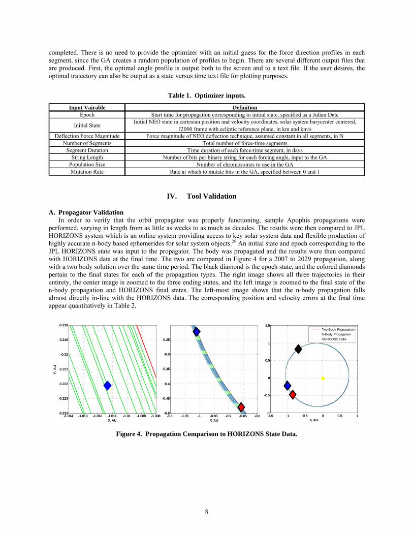
performed, varying in length from as little as weeks to as much as decades. The results were then compared to JPL HORIZONS system which is an online system providing access to key solar system data and flexible production of highly accurate n-body based ephemerides for solar system objects.26 An initial state and epoch corresponding to the JPL HORIZONS state was input to the propagator. The body was propagated and the results were then compared with HORIZONS data at the final time. The two are compared in Figure 4 for a 2007 to 2029 propagation, along with a two body solution over the same time period. The black diamond is the epoch state, and the colored diamonds pertain to the final states for each of the propagation types. The right image shows all three trajectories in their entirety, the center image is zoomed to the three ending states, and the left image is zoomed to the final state of the n-body propagation and HORIZONS final states. The left-most image shows that the n-body propagation falls almost directly in-line with the HORIZONS data. The corresponding position and velocity errors at the final time appear quantitatively in Table 2.

-1.014 -1.013 -1.012 -1.011 -1.01 -1.009 -1.008-0.224

-0.223

-0.222

-0.221

-0.22

-0.219

-0.218

X, AU

Y, A

U

-1.1 -1.05 -1 -0.95 -0.9 -0.85 -0.8-0.5

-0.45

-0.4

-0.35

-0.3

-0.25

X, AU-1.5 -1 -0.5 0 0.5 1-1

-0.5

0

0.5

1

1.5

X, AU

Two-Body PropagationN-Body PropagationHORIZONS Data

-1.014 -1.013 -1.012 -1.011 -1.01 -1.009 -1.008-0.224

-0.223

-0.222

-0.221

-0.22

-0.219

-0.218

X, AU

Y, A

U

-1.1 -1.05 -1 -0.95 -0.9 -0.85 -0.8-0.5

-0.45

-0.4

-0.35

-0.3

-0.25

X, AU-1.5 -1 -0.5 0 0.5 1-1

-0.5

0

0.5

1

1.5

X, AU

Two-Body PropagationN-Body PropagationHORIZONS Data

Figure 4. Propagation Comparison to HORIZONS State Data.

8

Table 2. Propagation Final State Comparison.

x (km) y (km) z (km) u (km/s) v (km/s) w (km/s)HORIZONS state -1.512949E+08 -3.322854E+07 -1.805093E+06 9.687389 -25.553659 1.595909

state -1.283081E+08 -7.172485E+07 7.092818E+05 18.443730 -22.353299 1.631328error 2.2987E+07 -3.8496E+07 2.5144E+06 8.756 3.200 0.035

error % -15.19% 115.85% -139.29% 90.39% -12.52% 2.22%state -1.512951E+08 -3.322804E+07 -1.805123E+06 9.687369 -25.553645 1.595908error -217.16 500.51 -30.45 -0.000021 0.000014 -0.000001

error % 0.0001% -0.0015% 0.0017% -0.0002% -0.0001% -0.0001%N-body

Two-body

B. Optimizer Validation The hybrid optimization algorithm was first tested by solving Rosenbrock’s valley function. This function is

often used as a benchmark for testing optimizers due to its nonlinear, analytic shape.27 The conjugate direction-based optimizer is capable of solving Rosenbrock’s function without the help of the GA, but employing the GA allows it converge in fewer steps. In order to verify that the algorithm works for asteroid deflection problems, the test cases from the following section were compared with a grid search over the entire design space. The grid searches were conducted first with low fidelity, and then re-performed around the best point with higher fidelity, on the order of 1° to 3°. In the interest of computation time, the grid searches were performed with only two segments, each 90 days long, while the optimizations were for six segments, each 30 days long. The grid search process was used to locate the global optimal solution to the fidelity of the discretization step in the search. Assuming that the thrust vector doesn’t vary greatly in the velocity-fixed reference frame, 90-day segments for the grid search should not greatly reduce the accuracy of the search. The grid search solutions are compared with the optimized results in Section V. In all three cases, optimal solutions showed excellent agreement with the grid search results. This indicates the optimization algorithm is functioning properly for these types of problems.

V. Test Cases In order to sufficiently test the optimization scheme, both short and long term Apophis deflection case studies

were performed. Finally, to demonstrate the tool was not tailored specifically to Apophis, a fictitious asteroid, D’Artagnan, was studied. D’Artagnan was initially created along with several other Earth impacting NEOs to evaluate various deflection techniques in support of the 2004 Planetary Defense Conference. Table 3 details the three test missions. D’Artagnan is unique from Apophis in that it actually is predicted to impact Earth on 4/1/2022. Therefore a simple miss distance change of a few kilometers is insufficient. Instead, the asteroid miss distance must be increased by thousands of kilometers to prevent the impact. For this reason, the thrust level for the D’Artagnan case has been increased to 10 N. This thrust is relatively high for most low-thrust techniques, but systems like mass drivers are capable of sustained forces exceeding 10 N.9 Smaller force magnitudes on the order of 0.1 to 1 N require a longer mission duration to divert D’Artagnan from its looming impact.

Table 3. Test case descriptions.

Case 1 Case 2 Case 3Asteroid Apophis Apophis D'ArtagnanDeflection Misson Start Date 1/1/2023 10/1/2028 1/1/2017Mission Duration, Days 180 180 180Available Thrust, N 0.1 1 10Impact/Close Approach Date 4/13/2029 4/13/2029 4/1/2022

For comparison, orbit parameters, mass, and size values of Apophis, D’Artagnan, and Earth in Table 4. The right

ascension of ascending node, argument of periapsis, and inclination of D’Artagnan were modified from the Planetary Defense Conference elements because they were initially designed via a two-body analytic solver. The true anomaly was also modified to reflect a 2017 detection and a 2022 impact instead of a 2004 detection and 2009 impact.

9

Table 4. Earth-asteroid comparison.

Earth Apophis D'Artagnana (AU) 1 0.922 0.902e 0.0167 0.191 0.302i (deg) 0 3.33 4.79ω (deg) 114 126 228Ω (deg) 349 205 191mass (kg) 5.97E+24 2.10E+10 2.70E+09radius (km) 6378 0.25 0.13

A. Case Study 1: Apophis Long Lead Time Deflection Mission The first test mission pertains to a deflection mission arriving at Apophis in January of 2023. It is assumed that

the mission lasts for six months, and utilizes a force of 0.1 N to maximize Apophis’ miss distance in its close approach in April of 2029. This thrust magnitude is easily achievable with an electric low-thrust propulsion system like the VASIMR.8 To discretize the problem, the 180-day mission was divided in to six equal 30-day segments. The optimizer converged on a solution shown in Table 5. The grid search-based optimal is also shown for comparison. Figure 5 depicts the thrust profile along the trajectory projected on to the ecliptic plane to better understand visually. The red vectors represent the thrust direction over the trajectory, which in this case are within a few degrees of the Apophis velocity vector. The mission begins at the green diamond, when the Earth is located at the blue diamond. The close approach occurs on April 13, 2029 at the black diamond.

As expected, the long lead-time case has an optimal solution very near to forcing directly in-line with the Apophis velocity vector over the entire six month period, since θ and φ are near to zero. The reason that these angles aren’t exactly zero is the lack of symmetry in n-body gravitational effects. Table 6 compares the miss distance with and without the deflection mission. The miss distance for a maximum orbit energy change, ∆ε, is also shown. This refers to a fixed deflection force along the velocity vector of Apophis. In other words, θ and φ are set to zero over the entire mission duration. By optimizing the force direction for this long lead-time mission, the close approach miss distance can be extended by approximately 130 m. Clearly for long lead time NEO deflection missions to maximize Earth miss distance, a force direction optimization may not be necessary.

Table 5. Case 1 optimal deflection angles and grid search comparison.

θ (deg) φ (deg) θ (deg) φ (deg)1 -2.17 -2.022 -1.87 -4.943 -2.18 0.694 3.76 -2.925 4.63 -3.046 1.51 -3.26

Optimized Deflection Grid Search Optimal

Segm

ent -1 -1

2 0

10

-1.5 -1 -0.5 0 0.5 1 1.5-1.5

-1

-0.5

0

0.5

1

1.5

X, AU

Y, A

U

Earth TrajectoryAsteroid Trajectory

Figure 5. Case 1 thrust profile and trajectory.

Table 6. Case 1 miss distance comparison.

rMD (km) rMD increase (km)No Deflection 38295.627

Maximum ∆ε Deflection 38334.23 38.61Optimized Deflection 38334.37 38.74

B. Case Study 2: Apophis Final Approach Deflection Mission A second Apophis case was studied to better understand the effect of lead time on the optimal thrust profile.

Again, this mission objective is to maximize miss distance. This case has a six month deflection mission that does not begin until October 1, 2028, six and a half months before the April 2029 close approach. Therefore the mission does not complete until a mere 14 days before the close approach. Here, the available thrust is assumed to be 1 N, since a 0.1 N force acting in such a short lead time case does not produce a substantial change in miss distance. The six-month mission was divided into six 30 day segments. The optimal thrust profile appears in Table 7, along with the corresponding trajectory in Figure 6. In this case, the optimizer’s value added over a maximum energy change thrust schedule is much greater. A deflection continuously in-line with Apophis’ velocity vector only produces a miss distance increase of 12 km. The miss distance change by utilizing the optimizer is 34% larger, as shown in Table 8.

This case reveals a flaw of the applied technique in discretizing the design space. The change in angle θ between legs 3 and 4 is significant. This shows up as a distinct discontinuity in the trajectory plot, which is likely non-optimal. By reducing the segment duration over the period of the mission when the optimal thrust angles are rapidly adjusting, a more optimal solution can be found. Through modification of the segment endpoints, a more continuous thrust angle profile could be converged upon, with a more optimal miss distance. For this case, the middle legs of the trajectory contain the largest variance in thrust angles. Therefore, the six thrusting segments were repartitioned such that the first 40 days were a single segment, and the final 60 days were a single segment. The remaining 80 days of the mission were equally divided for the four remaining segments, each 20 days. Figure 7 shows the optimal thrust profile and corresponding trajectory with the modified segment lengths. The thrust angles appear in Table 9. By modifying the thrust segment lengths, the maximum miss distance is extended by another 0.23 km, as shown in Table 8.

11

Table 7. Case 2 optimal deflection angles and grid search comparison.

θ (deg) φ (deg) θ (deg) φ (deg)1 -15.50 -0.262 -29.64 4.473 -28.50 -0.244 -89.86 -3.585 -97.09 1.866 -96.33 -0.14

Optimized Deflection

Segm

ent

Grid Search Optimal

6

6

-90

-22

-1.5 -1 -0.5 0 0.5 1 1.5-1.5

-1

-0.5

0

0.5

1

1.5

X, AU

Y, A

U

Earth TrajectoryAsteroid Trajectory

Figure 6. Case 2 thrust profile and trajectory.

Table 8. Case 2 miss distance comparison.

rMD (km) rMD increase (km)No Deflection 38135.63

Maximum ∆ε Deflection 38147.49 11.86Optimized Deflection 38151.47 15.85

Optimized Deflection, Modifed Segments 38151.70 16.08

Table 9. Modified case 2 optimal deflection angles.

θ (deg) φ (deg)1 40 -16.48 2.752 20 -40.29 -2.083 20 -39.52 0.334 20 -57.29 0.645 20 -79.92 0.506 60 -104.59 1.80

Optimized Deflection

Segm

ent

Duration (days)

12

-1.5 -1 -0.5 0 0.5 1 1.5-1.5

-1

-0.5

0

0.5

1

1.5

X, AU

Y, A

U

Earth TrajectoryAsteroid Trajectory

Figure 7. Modified case 2 thrust profile and trajectory.

C. Case Study 3: D’Artagnan Deflection Mission Finally, a mission to divert NEO D’Artagnan was devised. D’Artagnan’s orbit is more eccentric and more

inclined than Apophis. D’Artagnan is also an order of magnitude smaller than Apophis in mass. This mission to maximize D’Artagnan Earth miss distance is also unique in that D’Artagnan is on a trajectory that directly impacts Earth, and is not merely a close approach. In other words, the close approach miss distance is less than the radius of Earth. Therefore, the mission must not just expand the miss distance by a few kilometers, but must instead move it by thousands of kilometers. For this reason, the deflection mechanism is assumed to have a force of 10 N.

For this mission, the six month mission occurs about five years prior to the impact date. The optimal thrust profile and corresponding trajectory appear in Table 10 and Figure 8 respectively. Table 11 compares the miss distance achieved via optimization to the maximum energy change case. Similar to case 1, the extensive lead time causes the optimal solution to be very near to the maximum energy change solution.

Table 10. Case 3 optimal deflection angles and grid search comparison.

θ (deg) φ (deg) θ (deg) φ (deg)1 -0.66 -0.252 -0.27 0.143 0.05 -0.104 0.05 -0.305 -0.42 -0.266 -1.26 0.06

Optimized Deflection Grid Search Optimal

Segm

ent 0 0

-1 0

13

-1.5 -1 -0.5 0 0.5 1 1.5-1.5

-1

-0.5

0

0.5

1

1.5

X, AU

Y, A

U

Earth TrajectoryAsteroid Trajectory

Figure 8. Case 3 thrust profile and trajectory.

Table 11. Case 3 miss distance comparison.

rMD (km) rMD increase (km)No Deflection 3330.56

Maximum ∆ε Deflection 22988.68 19658.12Optimized Deflection 22990.03 19659.47

D. Test Case Summary The three test cases demonstrated the capabilities of the optimization algorithm with a variety of problems

pertaining to maximization of close approach miss distance. For missions with lead times on the order of several orbit periods prior to the close approach, the optimal thrust profile is generally within a few degrees of the maximum ∆ε solution. It should be noted that for some cases, it may be best to reduce the orbit energy of the asteroid, meaning the maximum ∆ε solution will be with thrusting opposite the NEO velocity. It was coincidence that the orbits of both Apophis and D’Artagnan require increases in orbit energy to maximize Earth close approach miss distance. For final approach cases, or cases with less than a single orbit period before the close approach, the optimal thrust profile is quite different from the maximum ∆ε solution. It is this type of case that benefits most greatly from the optimization algorithm.

VI. Future Work The test missions in this analysis are somewhat idealized and lack the degrees of freedom that a general low-

thrust mission would include. The thrust magnitude is held at a constant value. In most real missions, the thrust is either variable in magnitude, or can be switched on and off. To expand on this analysis, test cases could be run that have mission durations over several revolutions of the NEO’s orbit, and allow for variable thrusting. With this type of problem, the objective could be to minimize the thrust magnitude necessary to achieve a specific miss distance, instead of maximizing miss distance. The objective could also be to find the minimum total impulse solution. These scenarios would simulate a more realistic type of mission design. The downside to bringing in additional segments and the ability to modulate thrust is the increase in degrees of freedom of the problem. This directly translates to additional time to run the optimizer. However, the flexibility of the tool designed herein allows for simple variation of input variable types and objective functions. Therefore, this tool is capable of solving these higher degree of freedom problems given more substantial time for computing.

14

Another future task would be to add a visualization capability to the orbit propagator. Currently, all trajectory plots are generated via MATLAB using the text output files of the propagator. This can be a cumbersome task for the user, especially if many cases are being executed for a given analysis. JAVA scripting is known for its extensive visualization capabilities which have not been utilized. Also, plotting and visualization tools already exist within JAT, which may be tailored to this problem.

VII. Conclusion This analysis focused on the design and development of a unique tool for optimizing NEO deflection mission

trajectories. The core of this tool is a high fidelity long term orbit propagator native to JAVA. This propagator utilizes DE405 ephemeris data and an adaptive time step integration method to remain efficient yet accurate in propagating celestial bodies over long periods of time. The orbit propagator allows for additional forces to be input to the equations of motion to model deflection techniques.

Coupled with the high fidelity orbit propagator is a hybrid optimization algorithm designed to optimize a trajectory for a given set of variable inputs and objectives. Because low-thrust trajectory optimization often involves multi-modal behaviors, the algorithm first utilizes a genetic algorithm to locate the region in which the global optimum exists. Because the GA requires a discretization of the design space, the absolute optimal solution cannot be found directly. Instead, the genetic algorithm’s optimal solution is input to a second optimizer which is continuous in the design space. Utilizing Powell’s method, this conjugate gradient-based optimizer then finds the local minimum within the region output by the GA.

The optimization tool was tested via three cases. These cases varied in lead time prior to close approach, target asteroid, and allotted thrust magnitude. In general, the driving factor for the behavior of the optimal thrust profile was the lead time. Long lead time missions tended to have optimal profiles near the maximum energy change solution, while the short lead time mission featured a thrust profile that was nearly perpendicular to the velocity of the NEO for large portions of the mission. More extensive testing with variable thrust magnitudes and longer mission times would assist in further validating the tool and also provide more real-world examples of missions for which this tool could be utilized.

15

References 1Morrison, D., “The Spaceguard Survey,” Proceedings of the NASA International Near Earth Object Detection Workshop,

Pasadena, CA, 1992. 2Conway, B. A., “Near-Optimal Deflection of Earth-Approaching Asteroids,” Journal of Guidance, Control, and Dynamics,

Vol. 24, No. 5, 2001. 3Chesley, S. R., “Potential Impact Detection for Near-Earth Asteroids: The Case of 99942 Apophis (2004 MN4),” Proceedings

of the International Astronomical Union Symposium on Asteroids, Comets, and Meteors, No. 229, 2005. 4National Aeronautics and Space Administration, “Near-Earth Object Survey and Deflection Analysis of Alternatives,”

Washington, DC, URL: http://neo.jpl.nasa.gov/neo/report2007.html [cited 4 November 2007]. 5French, D. B., and Mazzoleni, A. P., “Use of Tethered Ballast Mass for Near Earth Object Collision Avoidance,” 43rd

AIAA/ASME/SAE/ASEE Joint Propulsion Conference & Exhibit, Cincinnati, OH, AIAA 2007-5430, 2007. 6Schaffer, M. G., Charania, A. C., and Olds, J. R., “Evaluating the Effectiveness of Different NEO Mitigation Options,”

Aerospace Corporation Planetary Defense Conference, Washington, DC, 2007. 7Lu, E. T., and Love, S. G., “Gravitational Tractor for Towing Asteroids,” Nature, Vol. 438, 10 Nov. 2005, pp. 177-178. 8Williams, B. G., Durda, D. D., and Scheeres, D. J., “The B612 Mission Design,” Planetary Defense Conference: Protecting

Earth from Asteroids, AIAA 2004-1448, 2004. 9Olds, J. R., Charania, A. C., and Schaffer M. G., “Multiple Mass Drivers as an Option for Asteroid Deflection Missions,”

Aerospace Corporation Planetary Defense Conference, Washington, DC, 2007, URL: http://www.aero.org/conferences/planetarydefense/2007papers/S3-7--Olds-Paper.pdf [cited 27 November 2007].

10Rayman, M. D., Varghese, P., Lehman, D. H., and Livesay, L. L., “Results from the Deep Space 1 Technology Validation Mission,” 50th International Astronautical Congress, IAA-99-IAA.11.2.01, Acta Astronautica 47, 2000.

11Brophy, J. R., Etters, M. A., Gates, J., Garner, C. E., Marlin, K., Lo, C. J., Marcucci, M. G., Mikes, S., Pixler, G., and Nakazono, B., “Development and Testing of the Dawn Ion Propulsion System,” 42nd AIAA/ASME/SAE/ASEE Joint Propulsion Conference & Exhibit, Sacramento, CA, AIAA 2006-4319, 2006.

12Sims, J. A., Finlayson, P. A., Rinderle, E. A., Vavrina, M. A., and Kowalkowski, T. D., “Implementation of a Low-Thrust Trajectory Optimization Algorithm for Preliminary Design,” AIAA/AAS Astrodynamics Specialist Conference and Exhibit, Keystone, CO, AIAA 2006-6746, 2006.

13Kowalkowski, T. D., Rinderle, E. A., “Mission-Analysis Low-Thrust Optimization (MALTO) Users Manual,” [CD-ROM] Version 1.0, Pasadena, CA, 2006.

14Biesbroek, R., “Swing-by Calculator – Software User Manual,” Issue 8, JAQAR Space Engineering, 2007. 15Sakai, T., “A Study of Variable Thrust, Variable Isp Trajectories for Solar System Exploration,” Ph. D. Dissertation, School

of Aerospace Engineering, Georgia Institute of Technology, Atlanta, GA, 2004. 16Russell, R. P., “Primer Vector Theory Applied to Global Low-Thrust Trade Studies,” Journal of Guidance, Control, and

Dynamics, Vol. 30, No. 2, March-April 2007. 17Bate, R. B., Mueller, D. D., and White, J. E., Fundamentals of Astrodynamics, Dover Publications, Inc., New York, 1971. 18Ma, C., Arias, E. F., Eubanks, T. M., Fey, A. L., Gontier, A. M., Jacobs, C. S., Sovers, O. J., Archinal, B. A., and Charlot, P.,

“The International Celestial Reference Frame as Realized by Very Long Baseline Interferometry,” The Astronomical Journal, Vol. 116, No. 1, Jul. 1998, pp. 516-546.

19Standish, E. M., “JPL Planetary and Lunar Ephemerides, DE405/LE405,” Jet Propulsion Laboratory Interoffice Memorandum 312.F-98-048, 26 August 1998.

20Barbee, B. W., Fowler, W. T., “Spacecraft Mission Design for the Optimal Impulsive Deflection of Hazardous Near Earth Objects using Nuclear Explosive Technology,” Aerospace Corporation Planetary Defense Conference, Washington, DC, 2007.

21JAT, Java Astrodynamics Toolkit, The University of Texas at Austin, URL: http://jat.sourceforge.net/ [cited 15 November 2007].

22Vallado, D. A., Fundamentals of Astrodynamics and Applications, 2nd ed., Microcosm Press, El Segundo, CA, 2001. 23Chesley, S. R., Ostro, S. J., Vokrouhlicky, D., Capek, D., Giorgini, J. D., Nolan, M. C., Margot, J., Hine, A. A., Benner, L. A.

M., and Chamberlin, A. B., “Direct Detection of the Yarkovsky Effect by Radar Ranging to Asteroid 6489 Golevka,” Science, Vol. 302, 5 December 2003, pp. 1739-1742.

24Goldberg, D. E., Genetic Algorithms in Search, Optimization, & Machine Learning, Adddison Wesley Longman, Inc., Reading, MA, 1989.

25Vanderplaats, G. N., Numerical Optimization Techniques for Engineering Design, 4th ed., Vanderplaats Research & Development, Inc., Colorado Springs, CO, 2005.

26Giorgini, J.D., Yeomans, D.K., Chamberlin, A.B., Chodas, P.W., Jacobson, R.A., Keesey, M.S., Lieske, J.H., Ostro, S.J., Standish, E.M., Wimberly, R.N., "JPL's On-Line Solar System Data Service", Bulletin of the American Astronomical Society 28(3), 1158, 1996.

27Chong, E. K. P., Zak, S. H., An Introduction to Optimization, 2nd ed., John Wiley & Sons, Inc., New York, 2001.

16