lower and upper bounds for positive linear functionals

LOWER AND UPPER BOUNDS FOR POSITIVE LINEAR

FUNCTIONALS

ALLAL GUESSAB

Abstract. This paper deals with the problem of finding lower and upper-

bounds in a set of convex functions to a given positive linear functional; thatis, bounds which estimate always below (or above) a functional over a family of

convex functions. A new set of upper and lower bounds are provided and their

extremal properties are established. Moreover, we show how such bounds canbe combined to produce better error estimates. In addition, we also extends

many results from [7], which hold true for simplices, to results for any convex

polytopes. Particularly, we use our result to obtain multivariate versions ofsome inequalities first given, respectively, by Favard in [3] and Hammer in

[14], over any convex polytope. For smooth (nonconvex) twice continuously

differentiable functions, we will also show how both the lower and upper boundscould be improved. Finally, we establish a general result concerning error

estimates. This seems to suggest a more unified and effective approach forproblems of this sort.

1. Introduction, notations and preliminary results

Let Ω be a convex polytope in Rd with (finite) set of (n + 1) distinct verticesVn = v0, . . . ,vn. Throughout this paper d and n denote positive integers suchthat n ≥ d. Let C(Ω) denote the class of all real-valued continuous functions on Ω.The set of all continuous convex functions defined on Ω will be denoted by K(Ω).A linear functional T which is defined on C(Ω) is called positive, if it takes non-negative values when applied to each nonnegative function in the set C(Ω). We saythat T is a normalized linear functional if T [1] = 1. We next denote by N∗(Ω) theset of all normalized positive linear functionals on C(Ω). We shall always assumethat the elements of N∗(Ω) are strictly positive on C(Ω), i.e. if T ∈ N∗(Ω) thenT [f ] > 0 whenever f(x) ≥ 0, and f is non-identically null continuous function onΩ.Throughout the paper, the symbol T will be reserved to denote a fixed normalizedpositive linear functional belonging to N∗(Ω).

The problem of lower and upper bounds of functionals in its most general formcan be described in the following way: Given T ∈ N∗(Ω), a common problem innumerical analysis is that of estimating T [f ] for some f in C(Ω). One popularnumerical approach is to replace T [f ] by an other simple approximating functional

Date: Received: January 17, 2012/ Accepted: June 9, 2012.2000 Mathematics Subject Classification. Primary 41A63, 41A80, 52A40, 65D30, 65D32; Sec-

ondary 26B25, 26D15, 52B11.Key words and phrases. Convex functions – Extremal properties – Delaunay triangulation–

Favard’s inequality–Lower and upper bounds–Polytopes–Positive linear functionals–Voronoidiagram.

1

sever

Typewriter

Received 06/02/13

2 ALLAL GUESSAB

A[f ], which can relatively easy to evaluate numerically. The key idea, to quantifythe quality of the numerical approximation A[f ] is to use two different functionalsbelonging to N∗(Ω), say L and R, to estimate the absolute value of the error|T [f ]−A[f ]| by |R[f ]− L[f ]| . If no other information is available, we are forced toaccept this (or some scaling of it) as the error estimate of |T [f ]−A[f ]|. However,to get a better estimate of T [f ], we need some a priori information about T in agiven subset G of C(Ω) (not necessarily containing f). A natural approach is toconstruct lower and upper bounding functionals L and R, such that

(1.1) L[g] ≤ T [g] ≤ R[g]

for any g ∈ G. We will sometimes use the terminology that T dominates L and Tis dominated by R on G.Hence, the following problem arises: We must select the functionals A,L,R, andalso decide how the deviation of A[f ] from T [f ] should measured. Obviously, if weknow that f belongs to the set G, we can sometimes better evaluate and estimateT [f ]. Indeed, if that is the case, we may take the approximation functional A :=(1 − λ)L + λR, any convex combination of L and R then, since inequalities (1.1)are satisfied by f , the error estimate can always be controlled as follows:

(1.2) |T [f ]−A[f ]| ≤ R[f ]− L[f ].

Equation (1.2), clearly, shows that when R[f ]−L[f ] is small, we are confident that|T [f ]−A[f ]| is also small. So we can know how closer our approximation is to theexact value. This procedure can still be used even if we do not know the exactvalue of T [f ].Therefore, we are interested in solving the following lower and upper bounds prob-lem:

• For a given subset G of C(Ω), a linear functional T and a function f ∈ C(Ω)determine two functionals L,R, in such a way that L ≤ T ≤ R on G.

The above problem is obviously too general to be dealt with under a unifyingaspect. From now on, we restrict ourselves to the case where the set G = K(Ω).Formally, the problem to be solved can be formulated as follows: Given a linearfunctional T in N∗(Ω).

• How to obtain upper and lower bounds L,R ∈ N∗(Ω) for T on K(Ω),namely,

(1.3) L[g] ≤ T [g] ≤ R[f ],∀g ∈ K(Ω)?

• Assume given lower and upper bounds. How to properly derive a procedureto be able to generate tighter lower and upper bounds?

The problem of finding lower and upper-bounds in a set of convex functions to agiven positive linear functional is a classical topic, there was a flourishing activityon this field even in the last ten years. For instance, it played a crucial role in ourresearch on the determination of the ‘best’ (or ‘optimal’) cubature formulae, see[7, 9, 10, 11, 13], where the latter problem has been extensively reviewed both fromthe theoretical study as well as the numerical point of view. Our aim in this paperis to merge and generalize the recent results from [7], which hold true for simplices,

LOWER AND UPPER BOUNDS FOR POSITIVE LINEAR FUNCTIONALS 3

to results for any convex polytopes.

A brief outline of the paper is : After establishing some preliminary definitionsand results about generalized barycentric coordinates and Jensen type inequalities,Section 2 provides lower and upper bounds in a set of convex functions to a givenpositive linear functional. In Section 3 we will discuss some extremal properties ofour upper and lower bounds. We will also obtain tighter lower and upper boundsby just using a simple averaging technique and combining those that are derived inSection 2. We will also extends many results from [7], which hold true for simplices,to results for any convex polytopes. Some of the arguments originate in [7], whileothers are our own. Consequently, we find an extension of a quadrature formulaover a finite interval first given by Hammer in [14], over any convex polytope. Asan application, in Section 4, we prove refinements, extensions and counterparts ofthe well-known Favard inequality. We also justify why we have limited our analysisto the case of polytopes. For smooth (nonconvex) twice continuously differentiablefunctions, Section 5 shows how both the lower and upper bounds given in Section2 could be improved. This section also establishes a general result concerning errorestimates.

The starting-point of this paper is the use of a Delaunay triangulation and there-fore do not resemble the proofs in [7], where the early techniques used were math-ematically rather simple. Furthermore, it is the power of Delaunay triangulationthat allows us to extend our results to all convex polytopes.

2. Lower and upper bounds of positive linear functionals

After establishing some notational conventions which will be used throughoutthe rest of the paper, this section focuses on the theoretical framework requisite forgenerating a new class of modified lower and upper bounds of a given normalizedpositive linear functional on K(Ω). We first recall some well known results ongeneralized barycentric coordinates and Jensen type inequalities. For a given T ∈N∗(Ω), let cgT (Ω) := (T [e1] , . . . , T [ed]), which we will call the center of gravitywith respect to the functional T in the polytope Ω. Here, we let e1, . . . , ed denotethe projections ei : x = (x1, . . . , xd) → xi. The so-called Jensen’s inequality forthe expectation of a convex real-valued function [17, p. 288] can be stated in thefollowing way: Let I ⊆ R be a (real) interval, and let f : I → R be a continuousconvex function on I. Let (Ω,A, µ) be a probability space, and let g : Ω→ I be aµ-integrable function over Ω. Then Eµ [g] ∈ I, Eµ [f(g)] exists, and it holds that

(2.1) f(Eµ [g]) ≤ Eµ [f(g)] ,

where Eµ denotes mathematical expectation with respect to the probability measureµ on Ω.The above inequality (2.1) was later generalized by McShane, see [16], as follows:Let f : Ω ⊆ Rd → R be a continuous convex function on the polytope Ω. Letgi ∈ C(Ω), i = 1, . . . , d, such that g(z) := (g1(z), . . . , gd(z)) ∈ Ω, for all z ∈ Ω, andf(g) ∈ L. Let us denote by T [g] := (T [g1], . . . , T [gd]). Then T [g] is in Ω, f(T [g]) isdefined and

(2.2) f (T [g]) ≤ T [f(g)].

4 ALLAL GUESSAB

Thus, if g is chosen to be the identity function on Ω, in the sense that Id(x) = x,then it follows from the above considerations that for any T ∈ N∗(Ω), we havealways cgT (Ω) ∈ int(Ω), and for any convex function f ∈ K(Ω) we have

(2.3) f (cgT (Ω)) ≤ T [f ].

Before we present our lower and upper bounds, we first prove some Lemmas ofgeneral usefulness. We begin by defining barycentric coordinates for an arbitrarysimplex.Given any linearly independent set Vn = v0, . . . ,vn of n+1 points in Rd, (d ≥ n),the simplex with the set of vertices Vn is the convex hull of Vn. If Ω is a simplex,and n = d, (e.g., a triangle in 2D or a tetrahedron in 3D), with vertices v0, . . . ,vd∈ Rd, then each point x of their convex hull Ω has a (unique) representation,that is there exist unique nonnegative real numbers λi(x), i = 0, . . . , d so that∑di= 0 λi(x) = 1, and x =

∑di= 0 λi(x)vi. The barycentric coordinates λ0, . . . , λd

are nonnegative affine functions on Ω, see [4, p. 288]. Note that a simplex is aspecial polytope given as the convex hull of n + 1 vertices, each pair of which isjoined by an edge.Barycentric coordinates also exist for more general types of polytopes, see Kalman[15, Theorem 2].

The next lemma without the property of affine independence is due essentiallyto Kalman [15]. Our statements are stronger than the ones provided in [15], butthe proof proceeds along the same lines as the proof in [15, Theorem 2], so we omitit. The most important fact of our extension is that one prescribed coordinate canbe chosen convex (or concave) on Ω. We claim no novelty for this result in theconvex case, which is proved in [15]. In fact, we have the following:

Lemma 2.1. Let Ω be a polytope in Rd, v0,v1, . . . ,vn its vertices. Then thereare affinely independent real continuous functions on Ω, ψ0, . . . , ψn, such that

(2.4)

n∑i=0

ψi(x) = 1, ψi(x) ≥ 0,

and

(2.5) x =

n∑i=0

ψi(x)vi.

Moreover, we can choose the barycentric coordinates ψ0, . . . , ψn in such a waythat one of them is convex or concave.

Warren [19] showed that ψ0, . . . , ψn can be chosen as rational functions, whichare uniquely determined if we require that each ψi have minimal degree. Later, wewill characterize the polytopes that have unique barycentric coordinates.

The next result gives lower and upper bounds for any functional T belonging toN∗(Ω).

Lemma 2.2. Let ψi, i = 0, . . . , n be defined as in Lemma 2.1. Let T ∈ N∗(Ω) andlet L,R ∈ N∗(Ω) such that

(2.6) L[f ] ≤ T [f ] ≤ R[f ],∀f ∈ K(Ω),


then for any f ∈ K(Ω) we have

(2.7) f(cgT (Ω)) ≤ L[f ] ≤ T [f ].

Moreover, if Ω is a simplex, then for any f ∈ K(Ω) we have

(2.8) T [f ] ≤ R[f ] ≤n∑

i= 0

ψi(cgT (Ω))f(vi).

Proof. Since the projection functions ei and −ei are both convex, then it followsfrom inequalities (2.6) that the centers of gravity cgL(Ω), cgT (Ω), cgR(Ω) coincide.Thus, we get from McShane inequality (2.3) that for all f ∈ K(Ω)

(2.9) f(cgT (Ω)) = f(cgL(Ω)) ≤ L[f ].

This shows the left-hand-side of the inequality in (2.7). Next we apply f on bothsides of linear precision (2.5) and make use of the convexity, we arrive at:

f(x) ≤n∑i=0

ψi(x)f(vi),

and so apply R of both sides gives for all convex function f ∈ K(Ω)

(2.10) R[f ] ≤n∑i=0

R [ψi] f(vi),

where in the last inequality, we have used linearity and positivity of R. The aboveinequality implies, once again, in view of the fact that ei and −ei are both convex:

(2.11) cgR(Ω) =

n∑i=0

R [ψi]vi.

Let us observe that cgT (Ω) has also the following two representations

cgT (Ω) =

n∑i=0

T [ψi]vi(2.12)

=

n∑i= 0

ψi(cgT (Ω))vi,(2.13)

where in the last equality we have used the identity (2.5) and the fact that cgT (Ω)is an interior point of Ω. But, the centers of gravity cgT (Ω) and cgR(Ω) coincide,then the uniqueness of barycentric coordinates for simplices guarantees that we canwrite

(2.14) R [ψi] = T [ψi] = ψi(cgT (Ω)),∀i = 0, . . . , n.

This, combined with (2.10) shows the left-hand inequality in (2.8) and completesthe proof Lemma 2.2.

Let us note that trivial upper and lower worst-case bounds are easiest to find ifthe functions is continuous only, since for any T ∈ N∗(Ω) and f ∈ C(Ω), we have

(2.15) infx∈Ω

f(x) ≤ T [f ] ≤ maxx∈Ω

f(x).

In order to generate ‘good’ lower and upper bounds, than those given by Lemma 2.2and in inequalities above, we need to subdivide the polytope Ω. From a numerical

6 ALLAL GUESSAB

Figure 1. The left figure is a Voronoi diagram with Ci is theVoronoi region associated to vertex vi. C(y) is the Voronoiregion associated to y. The right figure shows the associatedDelaunay triangulation. Ti, 1, . . . , 4, are the simplices of thetriangulation.

point of view, the precise effective lower and upper bounds in which we shall bechiefly interested here are those in which we chose ai, bi and xi so that:

m∑i= 0

aif(xi) ≤ T [f ] ≤m∑i= 0

bif(xi),∀f ∈ K(Ω),

where ai, bi are positive numbers and xi are some points in the polytope Ω.

Let y be an arbitrary but fixed point in int(Ω). With a slight abuse of notation,we will sometimes denote by vn+1 the point y. We shall then define, when Vn isthe set of all vertices of the polytope Ω,

Y := V ∪ y = v0, . . . ,vn,vn+1 .

For any z ∈ Y , we denote by VY (z) the (Euclidean) Voronoi region of z withrespect to the point set Y , that is the region consisting of all points of Ω that arecloser to z than to any other point in Y \ z,

VY (z) = x ∈ Ω : ‖x− z‖ ≤ ‖x− p‖ for all p ∈ Y \ z ,

where ‖.‖ is the (usual) Euclidean norm in Rd. The set of all Voronoi regions for allVY (z), z ∈ Y forms the Dirichlet-Voronoi diagram of Y. Dirichlet-Voronoi diagramsare also called Voronoi diagrams, Voronoi tessellations, or Thiessen polytopes. Fol-lowing common usage, we will use the terminology Voronoi diagrams. It is easy tosee that all of the Voronoi regions VY (z), z ∈ Y are (non-empty) convex polytopes,and their union is Ω. Furthermore, the interiors of VY (z), z ∈ Y are disjoint convexsets. A triangulation of Ω with respect to Y is a partition of Ω into a finite numberof d-dimensional simplices such that the vertices of which are points of Y and anytwo of them are either disjoint or meet in a common lower dimensional simplex.There is a very natural triangulation DT (Ω) of Ω, that uses only the points of Y astriangulation vertices and such that any simplex in DT (Ω) has y as a vertex. Sucha triangulation exists and it is called a Delaunay triangulation of Ω with respect toY and it can be obtained as the geometric dual of the Voronoi diagram of Y, see, e.g., [6]. It is a triangulation of Ω with respect to Y such that no point of Y is insidethe hyper circumsphere of any simplex of the triangulation, see Figure 1 in thecase when the domain Ω is a rhombus. Alternatively, such a triangulation can alsobe characterized by an approximation problem; see [2, Theorem 2.3]. Uniquenessof Delaunay triangulations is guaranteed if no d + 1 points of Y lie on a commonhyperplane in Rd and no d+ 2 points lie on a common hypersphere.

Let y ∈ int(Ω) and let Sy1 , . . .Sym be the simplices of DT (Ω) with respect the

set of points Y and let Ni be the set of all integers j such that vi is a vertex of Syj .

If x ∈ Syj and j ∈ Ni, then we denote by λyij(x) the barycentric co-ordinate of x


with respect to vi for the simplex Syj . It is easily verified that if x ∈ Syj ∩Syk , then

λyij(x) = λ

yik(x) if j, k ∈ Ni and λij(x) = 0 if j ∈ Ni, k 6∈ Ni. Therefore, setting

φyi (x) :=

λyij(x) if x ∈ Syj and j ∈ Ni0 otherwise,

for i = 0, . . . , n+ 1, we trivially obtain a set of well-defined functions, which are ageneralization of barycentric coordinates when Ω is a simplex. We list some basic

properties of the functions φy0 , . . . , φ

yn+1, of which the following are particularly

relevant to us:

(1) They are well-defined, piecewise linear and nonnegative real-valued contin-uous functions.

(2) They send Ω to the unit interval [0, 1].

(3) They form a partition of unity, so∑n+1i=0 φ

yi ≡ 1.

(4) The function φyi has to equal 1 at vi and 0 at all other points in Y \ vi,

i.e., φyi (vj) = δij ( δ is the Kronecker delta).

(5) They satisfy the linear precision property, that is,

(2.16) x =

n+1∑i=0

φyi (x)vi.

Since any simplex in DT (Ω) contains y as a vertex, to simplify notation from here

forward, we shall write φyn+1 simply as

φyn+1(x) :=

λyj (x) if x ∈ Syj and j ∈ 1, . . .m

0 otherwise,(2.17)

here m is the number of simplices in DT (Ω) and λyj (x) is the barycentric co-

ordinate of x with respect to y for the simplex Syj , (see Figure 1).

Kalman showed in [15, Theorem 2] that, for any given finite set x1, . . . ,xl ofpoints of Rd we can assign barycentric coordinates λ1, λ2, . . . , λl to their convexhull X in such a way that each coordinate is continuous on X and that one pre-scribed coordinate is convex on X. He does not identified exactly which barycentriccoordinate function has this property. Kalman also asked if whether it is alwayspossible to make all the coordinates convex simultaneously (see [15, Example 3]).Fuglede [5] answered this question by showing that if all the barycentric coordinatesare convex (or if they are all concave), then they are all affine, and consequently,X must be a simplex.

With these important general facts in mind, we now complement the Kalmanresult. The next Lemma shows that in our situation, for any fixed y ∈ int (Ω), the

function 1−φyn+1 (assigned to the point y) is convex: This convexity property willbe an important key to establish some extremal properties of our lower and upperbounds. Thus, the first main point of this paper is the following result, which wewill have several occasions to use.

8 ALLAL GUESSAB

Lemma 2.3. For any y ∈ int(Ω), the function 1 − φyn+1 is a convex continuouspiecewise-linear function on Ω and for i = 1, . . . ,m satisfies the identity:

(2.18)1

vol(Syi )

∫Syi

φyn+1(x) dx =

1

d+ 1=

1

vol(Ω)

∫Ω

φyn+1(x)dx.

Proof. First we show that −φyn+1 can be expressed as the maximum of a finite set

of affine functions. To this end let Syj be any fixed simplex in DT (Ω). We begin

by observing that for any i = 1, . . . ,m, λyi is nonnegative (affine function) on Ω.

To see that, it suffices to note that, for any fixed i, λyi (y) = 1 and λ

yi (x) = 0 is a

supporting hyperplane for Ω. Recall that an affine function is uniquely determinedby its values at the vertices of the simplex. For any fixed i = 1, . . . ,m, define the

functions dj , j = 1, . . .m, by dj = λyi − λ

yj , then a simple inspection shows that dj

is nonnegative on Syj . Hence h(x) := max−λy1 (x), . . . ,−λym(x)

= −λyi (x) for

all x ∈ Syi . Thus, it follows that for all i the restriction of h to Syi coincides with

the function −φyn+1. But now, h and −φyd+1 are identically equal in Ω, we then

get that −φyn+1 is convex, because affine functions are convex and the maximum of

convex functions is a convex function. This means that, 1 − φyn+1 is convex, sinceit is the sum of two convex functions.To show the left-hand inequality in (2.18), we use the identity (2.17), for the simplex

Syi , to find that

(2.19)

∫Syi

φyn+1(x) dx =

∫Syi

λyi (x) dx =

vol(Syi )

d+ 1

∑vλyi (v),

where the sum is taken over all vertices of the simplex Syi . The last identity can

be deduced using [13, Theorem 2.2] applied to the simplex Syi . Therefore, the

Kronecker delta property implies the desired result. Finally, a simple computationnow shows that adding inequalities (2.19) for i = 1, . . . ,m, and dividing by vol(S),yields the second desired equality in (2.18).

It should be noted a remarkable fact that integral identities (2.18) are indepen-dent of y and i. This property will be used later in some proofs.

Now we can state and prove our improved lower and upper bounds. We continueto denote vn+1 the point y. The next result is a main result in this section.

Theorem 2.4. Let y ∈ int(Ω) be fixed. Then, for any T ∈ N∗(Ω) and f ∈ K(Ω)the following inequalities hold

(2.20) f (cgT (Ω)) ≤ Ly [f ] :=

n+1∑i=0

Ayi f(x(φyi

))≤ T [f ] ≤ Ry [f ] :=

n+1∑i=0

Ayi f(vi),

with for any i = 0, . . . , n+ 1, Ayi = T

[φyi

]and

(2.21) x(φyi

)=

T[φyi e1

]T[φyi

] , . . . ,T[φyi ed

]T[φyi

] , (i = 0, . . . , n).


Moreover, if Ω is a simplex, then for any i = 0, . . . , n,

(2.22) Ayi =

(1− ψi(y)

ψi(cgT (Ω))Ayn+1

)ψi(cgT (Ω)).

Proof. In order to obtain the estimation from below (2.20), let us first observe thatthe center of gravity cgT (Ω) can be expressed as a convex combination of the points

x(φyi

). Indeed, it follows from the definition of cgT (Ω) and the partition of unity

functions φyi , i = 0, . . . , n+ 1 that cgT (Ω) =

∑n+1i=0 T

[φyi

]x(φyi

). Let f ∈ K(Ω),

then, the convexity of f implies that

f (cgT (Ω)) ≤n+1∑i=0

T[φyi

]f(x(φyi

)).

This shows the left-hand inequality of (2.20).We now prove the second inequality in (2.20). Let us define first the functionals onC(Ω) by

(2.23) Ti[g] =T[φyi g]

T[φyi

] , (i = 0, . . . , n+ 1).

Now it is easily seen that for all i, the functional Ti belongs to N∗(Ω), and its

center of gravity is x(φyi

). Thus, according to Jensen’s inequality (2.7) applied

to the functional Ti instead of T , it follows from the definition of cgTi(Ω) that

cgTi(Ω) := x

(φyi

). Moreover, we have for all f ∈ K(Ω)

(2.24) T[φyi

]f(x(φyi

))≤ T

[φyi f].

Summing up for i = 0, 1, . . . , n + 1, and taking into account that the functions

φyi , i = 0, . . . , n + 1, form a partition of unity, we get the desired result. Let us

mention that the left-hand inequality of (2.20) can also be proved by using Lemma2.2 and the inequality we just proved.To obtain the estimate from above, we first observe that equation (2.16) tells usthat any point x ∈ Ω can be written as convex combination of the extreme pointsof Ω and the point y ∈ Ω, then if we apply f on both sides of (2.16) and make useof the convexity, we get

f(x) ≤n∑i=0

φyi (x)f(vi) + φ

yn+1(x)f(y).

So by applying T of both sides of the above equation and using the linearity andpositivity properties of T , we get the desired result. Again, linear precision (2.16)implies that the center of gravity cgT (Ω) can also be expressed as follows:

cgT (Ω) =

n∑i=0

T[φyi

]vi + T

[φyd+1

]y.

But also by Lemma 2.1 we may write y =∑ni=0 ψi(y)vi, then we have immediately

cgT (Ω) =

n∑i=0

(T[φyi

]+ T

[φyd+1

]ψi(y)

)vi.

10 ALLAL GUESSAB

Thus, using the uniqueness of barycentric coordinates for a simplex, we concludethat

(2.25) ψi(cgT (Ω)) = T[φyi

]+ T

[φyn+1

]ψi(y), (i = 0, . . . , n).

This prepares us for the final part of the proof of the theorem. Indeed, the aboveequation immediately yields

(2.26) T[φyi

]=

(1− ψi(y))

ψi(cgT (Ω))Ayn+1

)ψi(cgT (Ω)), (i = 0, . . . , n).

This shows identities (2.22), and the proof is complete.

Remark 2.5. It should be noted that for any point y in the interior of Ω, Lemma2.2 tells us that if Ω is a simplex, then the upper bound given in Theorem 2.4 mustbe better on K(Ω) than that those given by (2.8) of Lemma 2.2. This can also beeasily verified directly.

Before we proceed further, we would like to remark that under uniqueness ofbarycentric coordinates, the reader should note that inequality (2.8) and the rightinequality (2.20) with coefficients as given in (2.22) remain valid. This result moti-vates a question about polytopes with a related property. Let us raise the following:

Problem 2.6. For which polytopes Ω in Rd, the barycentric coordinates given inlemma 2.1 are uniquely defined?

The following Lemma shows that unfortunately the only polytopes with thisproperty are the simplices. More precisely, we have the following characterization:

Lemma 2.7. Let Ω be a polytope in Rd, with n+ 1 vertices v0, . . . ,vn , (n ≥ 1).Then, the following properties of Ω are equivalent

(1) Ω is a simplex;(2) The barycentric coordinates with respect to the vertices of Ω are unique.

Proof. The proof sketch is as follows: Given a simplex Ω with vertices v0, . . . ,vn .By Lemma 2.1, there must exist at least one barycentric coordinate system on Ω,ψ0, . . . , ψn, such that for all x ∈ Ω we have

(2.27)

n∑i=0

ψi(x) = 1, ψi(x) ≥ 0,

and

(2.28) x =

n∑i=0

ψi(x)vi.

For any x ∈ Ω, we can calculate ψi(x) by defining M to be the d × n matrixv1 − v0, . . . ,vn − v0, and solving the equation

x− v0 = M (ψ1(x), . . . , ψn(x))T,

where (ψ1(x), . . . , ψn(x))T

is the transpose of the row vector (ψ1(x), . . . , ψn(x)) .Recall that our definition of a simplex stated that its vertices are linearly inde-pendent points, then the matrix M is assumed to have full column rank, and


Figure 2. This figure gives an example of a triangulation usingonly the vertices of the polytope.

consequently the following system of linear equations has a unique solution givenby

(ψ1(x), . . . , ψn(x))T = (MTM)−1M(x− v0),

with ψ0(x) = 1 −∑ni=1 ψi(x). This shows that the barycentric coordinates of a

point are uniquely determined by the vertices of the simplex in question. In orderto prove the converse assume the contrary, namely that Ω is not a simplex. We firstobserve that, if n is less than or equal to 2 then we have nothing to prove, sinceΩ is already a simplex. Here we used the fact that Ω is assumed to be describedby n+ 1 vertices. Thus without loss of generality we may assume that n is greaterthan or equal to 3. The polytope Ω admits at least one triangulation T in whichevery vertex is an extreme point of Ω, see [5, Theorem 2]. Note that since Ω is nota simplex, and n is greater than 3, then T has at least two adjacent simplices, sayS and S′. Denote by F the common facet of S and S′, and v (respectively v′) thevertex of S (respectively S′), lying in opposite the facet F , see Figure 2. Since,T does not use any interior points, then S ∪ S′ is a convex polytope with verticesnecessarily among those of Ω. Consequently the line segment joining the two pointsv and v′ meets F in at least one point, say y. Thus, there is a common point y inthe interiors of the two different simplices F and [v,v′], and then y must have twodifferent sets of barycentric coordinates. This contradicts the uniqueness propertyfor the barycentric coordinates and shows that Ω must be a simplex.

In order to simplify the notation, in what follows we denote byAcgn+1 = T[φcgT (Ω)n+1

],

and for any i = 0, . . . , n, φcgi = φcgT (Ω)i . By using these notations, if the domain is

a simplex Theorem 2.4 tells us the following:

Corollary 2.8. Let Ω be a simplex and let

Lcg [f ] := (1−Acgn+1)

n∑i=0

ψi(cgT (Ω))f (x (φcgi )) +Acgn+1f(x(φcgn+1

))Rcg [f ] := (1−Acgn+1)

n∑i=0

ψi(cgT (Ω))f(vi) +Acgn+1f(cgT (Ω)).

Then the following inequality is valid for any f ∈ K(Ω)

LcgT (Ω)[f ] ≤ T [f ] ≤ RcgT (Ω)[f ].

Remark 2.9. Let us denote by K+(Ω) the set of nonnegative convex functionsbelonging to K(Ω). It should be noted that under the hypotheses of Corollary 2.8,the functional T is bounded from below on K+(Ω) by

(2.29) Lcg [f ] := (1−Acgn+1)

n∑i=0

ψi(cgT (Ω))f (x (φcgi )) .

Indeed, recalling inequalities (2.24), we can see that, for all i = 0, . . . n,

(1−Acgn+1)ψi(cgT (Ω))f (x (φcgi )) ≤ T [φcgi f ],

12 ALLAL GUESSAB

and then summing up the above inequalities, we have immediately for all functionfrom K+(Ω)

Lcg [f ] ≤ T [(1− φcgn+1)f ]

= T [f ]− T [φcgn+1f ],

and consequently it follows that LcgT [f ] ≤ T [f ]. But obviously we have Lcg[f ] ≤Lcg[f ], for all f ∈ K+(Ω), then the functional Lcg is an improvement of the lower

bound Lcg on K+(Ω).By analogy, we can write the expression for Rcg as follows:

Rcg [f ] = Rcg −Acgn+1

(n∑i=0

ψi(cgT (Ω))f(vi)− f(cgT (Ω))

),

where Rcg [f ] :=∑ni=0 ψi(cgT (Ω))f(vi). Then, Lemma 2.2 informs us that the

functional Rcg is an upper bound for T on K(Ω). Since we have subtracted anonnegative term, then Rcg appears here as an improvement for the upper boundRcg. But this time, the improvement is valid for any continuous convex function.

In particular, if T is the functional-integral over a simplex, Corollary 2.8 allowsus to extend a quadrature formula over an interval, first given by Hammer in [14], toa multivariate setting. This result was first proved in [7]. Indeed, as a consequenceof the above result combined with Lemma 2.3, we immediately obtain the following:

Corollary 2.10. Let Ω ⊂ Rd be a simplex with vertices v0, . . . ,vd and center ofgravity v∗ = v0+...+vd

d+1 . Set

Lcg [f ] :=1

d+ 1

(d

d+ 1

d∑i=0

f

((v∗ − vid+ 1

)+ v∗

)+ f(v∗)

)

Rcg[f ] :=1

d+ 1

(d

d+ 1

d∑i=0

f(vi) + f(v∗)

).

Then for every convex function from K(Ω), we have

(2.30) Lcg [f ] ≤ 1

vol(Ω)

∫Ω

f(x) dx ≤ Rcg[f ].

Proof. Just apply the integral identity (2.18) proved in Lemma 2.3.

3. Refinement and comparison of our upper and lower bounds

The aim of this section is to establish some extremal properties of the upperand lower bounds given by Theorem 2.4. We will also get ‘better’ lower and upperbounds by just combining those that are derived in Section 2.

The next Theorem describes relevant properties of the upper bound derived inTheorem 2.4. In what follows Ry denotes the upper bound derived in Theorem 2.4.This extends to arbitrary polytopes in Rd, a result in [7] in the case of a simplex.

Theorem 3.1. Let T ∈ N∗(Ω),y ∈ int(Ω), Ayn+1 = T [φ

yn+1]. Suppose that there

are positive real numbers B0, . . . , Bn+1 such that their sum is 1, and for every


f ∈ K(Ω), we have

(3.1) T [f ] ≤ R[f ] :=

n∑i=0

Bif(vi) +Bn+1f(y).

Then,

(3.2) Bn+1 ≤ Ayn+1.

Moreover, if Ω is a simplex, then equality in (3.2) is attained if and only if the

two functionals R and Ry are identically equal. If Bn+1 > Ayn+1 then T cannot

bounded by R on K(Ω).

Proof. Fix y ∈ int(Ω), then by Lemma 2.3, we already know that the function

1 − φyn+1 ∈ K(Ω). Recall that φyn+1 takes the value 1 at y and vanishes on all

vertices of Ω. Consequently, taking into account that the two functionals T and Rcoincide over the set of constant functions, we get from dominant property (3.1) onK(Ω)

−Ayn+1 = T [−φyn+1] ≤ R[−φyn+1] = −Bn+1φyn+1(y) = −Bn+1.

Hence, for every y ∈ int(Ω) we have Bn+1 ≤ Ayn+1. If, moreover, Ω is a simplex,

the sufficiency condition is obvious. For this, it suffices to consider the equality

condition for the the function φyn+1. It remains to show that if Bn+1 = A

yn+1 then

R = Ry . To this end, since, T is dominated by R and Ry on K(Ω) and affinefunctions and their opposites belong to K(Ω), then the functionals R and Ry havethe same center of gravity. Therefore, we have

cgT (Ω) =

n∑i=0

Ry [ψi]vi(3.3)

=

n∑i=0

R [ψi]vi,(3.4)

here ψi, i = 0, . . . , n are the barycentric coordinates defined in Lemma 2.1. Be-cause of the uniqueness of barycentric coordinates we get

R[ψi] = Ry [ψi],

then clearly Bi + Bn+1ψi(y) = Ayi + A

yn+1ψi(y). Finally, since Bn+1 = A

yn+1, we

get Bi = Ayi . Thus, we see that R = Ry .

In order to complete the proof we have to find a function h ∈ K(Ω) for which

inequality (3.1) is not true. To this end, assume that Bn+1 > Ayn+1, then since

Bn+1 = R[φyn+1],(3.5)

Ayn+1 = T [φ

yn+1],(3.6)

it follows that inequality (3.1) does not hold for the convex function −φyn+1 ∈ K(Ω).

This contradiction shows that Bn+1 cannot strictly bigger than Ayn+1 and completes

the proof of the theorem.

The arguments in Theorem 3.1 generalize easily to yield the following moregeneral result:

14 ALLAL GUESSAB

Remark 3.2. Assume that R[f ] :=∑ni=0Bif(vi)+Bn+1f(y) dominates T on K(Ω),

then the equality R = Ry holds true if and only if there exists an index i belonging

to 0, . . . , n+ 1 such that Ayi = Bi (here, Ry is the functional defined in (2.20)).

This extends Theorem 3.1.

Before we go on to our next result, we need yet some more preparation. Werecall that a partition of unity pini=0 consists of a finite collection of continuousfunctions from Ω to the unit interval [0, 1] and whose values sum the unity for allx ∈ Ω. For a partition of unity pi, i = 0, . . . , n, we simply write p and say thatit is a pu-system. The collection of all pu-systems will be denoted by P n+1. Ify0, . . . ,yn denote (n + 1)-points in Ω and B0, . . . , Bn be (n + 1)-nonnegative realnumbers such that their sum is 1, let us define

(3.7) R[f ] :=

n∑i=0

Bif(yi).

Let T ∈ N∗(Ω), we will assume throughout that for any p := pi, i = 0, . . . , n ∈P n+1, we have T [pi] > 0, i = 0, . . . , n. For a given functional R of the form (3.7),we will say that R is generated by a pu-system with respect to T if there exists apu-system p = pi,= 0, . . . , n, such that

Bi = T [pi] and yi = cgTi(Ω) :=

(T [pie1]

T [pi], . . . ,

T [pied]

T [pi]

), (i = 0, . . . , n),

where Ti is the functional defined on C(Ω) by Ti[f ] = T [pif ]T [pi]

.

The next result gives a necessary and sufficient condition under which any func-tional of the form (3.7) is bounded from above by T on K(Ω).

Theorem 3.3. Let B0, . . . , Bn be (n+ 1)-nonnegative real numbers such that theirsum is 1. For any y0, . . . ,yn, (n+ 1)-points in Ω, define

R[f ] :=

n∑i=0

Bif(yi).

Then R is generated by a pu-system with respect to T if and only if R is boundedabove by T on K(Ω).

Proof. Main idea of the proof. Similar arguments show that Theorem 2.4 also holds

when replacing the barycentric coordinates systemφy0 , . . . , φ

yn

by any pu-system.

Hence, if R is generated by a pu-system then R is bounded from above by T onK(Ω). The difficulty is contained in the converse implication, but it can be provedby an easy adaptation of [8, Theorem 3.8] to the more general setting of positivelinear functionals. We leave the details to the reader.

As a corollary we obtain the following result:

Corollary 3.4. Let Ω be a polytope in Rd and v0,v1, . . . ,vn its vertices. Forany y ∈ Ω, define

R[f ] :=

n∑i=0

Bif(vi) +Bn+1f(y).

Then the functional T is bounded above by R on K(Ω) if and only if B0 = . . . =Bn = 0, Bn+1 = 1, and y = cgT (Ω).


Proof. The proof of this corollary is a standard consequence of Theorem 3.3. Thedetails are as follow. Assume that T is dominated by R on K(Ω), then, by Theorem3.3, R is generated by a pu-system p := pi, i = 0, . . . , n , with

vi =

(T [pie1]

T [pi], . . . ,

T [pied]

T [pi]

), (i = 0, . . . , n).

As the centers of gravity(T [pie1]T [pi]

, . . . , T [pied]T [pi]

), (i = 0, . . . , n), are interior points,

this is possible only if B0 = . . . = Bn+1 = 0, Bn+2 = 1, and y = cgT (Ω).The converse implication can be proved by using Lemma 2.2.

In order to compute better lower and upper bounds, as suggested early in theIntroduction, we take a convex combination of nonnegative coefficients of lowerand upper bounds, given by Theorem 2.4. The next result gives all admissible

convex combinations. For simplicity we continue to denote Acgi = T[φcgT (Ω)i

], i =

0, . . . , n+ 1.

Theorem 3.5. Let us define the two linear functionals Lcg and Rcg by

Lcg [f ] := f(cgT (Ω))

Rcg [f ] :=

n+1∑i=0

Acgi f(vi).

For any α ∈ [0, 1] , let us set

Tα[f ] := (1− α)Lcg [f ] + αRcg [f ] .(3.8)

Then,

(1) Tα is dominated by T on K(Ω) if and only if α = 0;(2) T is dominated by Tα on K(Ω) if and only if α = 1.

Proof. (1) is an immediate consequence of Corollary 3.4. To prove (2), let us assumethat T is dominated by Tα on K(Ω). Then, since −φcgn+1 belongs to K(Ω), it takesthe value −1 at cgT (Ω) and vanishes on all vertices of Ω, we have

−Acgn+1 = T [−φcgn+1] ≤ Tα[−φcgn+1] = −(1− α)− αAcgn+1,

here, for simplicity in notation, we have denoted φcgT (Ω)n+1 by φcgn+1. This shows that

(1− α)(1−Acgn+1) ≤ 0.

According to the fact, that Acgn+1 is strictly less than or equal to 1 and α ∈ [0, 1], itfollows that the above inequality is satisfied only if α = 1. The converse implicationis obvious, since for α = 1, T1 := Rcg and by Theorem 2.4, T is dominated by Rcg

on K(Ω).

Now consider the case when the domain Ω is a simplex. In this case, Lemma 2.2implies that for all α ∈ [0, 1]

Lcg [f ] ≤ Tα[f ] := (1− α)Lcg [f ] + αRcg [f ] ≤ Rcg [f ] ,∀f ∈ K(Ω),

where Lcg and Rcg are defined by

Lcg [f ] := f(cgT (Ω))

Rcg [f ] :=

n∑i=0

ψi(cgT (Ω))f(vi).

16 ALLAL GUESSAB

The problem we wish to consider is: For which values of α ∈ [0, 1], is T boundedfrom below or above by Tα on K(Ω)?

The following Theorem gives all admissible values of α for which Tα is boundedbelow by T on K(Ω).

Theorem 3.6. If Ω is a simplex then the following inequalities hold for everyα ∈

[Acgn+1, 1

]:

(3.9) T [f ] ≤ Tα[f ],∀f ∈ K(Ω).

Moreover, as a function of α, Tα is non-decreasing on[Acgn+1, 1

]. In addition, if

α > Acgn+1, then Tα cannot dominate T on K(Ω).

Proof. A simple inspection of Theorem 2.4 shows that (3.9) holds for α = Acgn+1.Since, by Lemma 2.2, we know already that Lcg is dominated by Rcg, (note thatthis inequality is also a very easy consequence of the classical Jensen’s discreteinequality for convex functions), it follows that Tα is a non-decreasing function ofα and that (3.9) holds for each α ∈

[Acgn+1, 1

]. The rest of proof can be carried out

similarly as in Theorem 3.1.

We can show similarly as in the proof of Theorem 3.6 that Tα is dominated byT on K(Ω) if and only if α = 0.

We naturally asked if a similar result of Theorem 3.6 holds for convex com-binations of lower bounds given in Theorem 2.4. To this end, it is also worthemphasizing the following result:

Theorem 3.7. Let us define the functional Uα on C(Ω) by

Uα [f ] = (1− α)f(x(φcgn+1

))+ α

n∑i=0

ψi(cgT (Ω))f (x (φcgi )) .

Then if Ω is a simplex the following inequalities hold for every α ∈[0, Acgn+1

]:

(3.10) Uα[f ] ≤ T [f ],∀f ∈ K(Ω).

Moreover, as a function of α, Uα is non-decreasing on[0, Acgn+1

]. In addition, if

α > Acgn+1, then Uα cannot dominated by T on K(Ω).

Proof. The proof is similar to the proof of Theorem 3.6, and it is only necessary touse the second inequality obtained in Theorem 2.4.

4. A generalization of J. Favard’s inequality

Let us now turn to some applications of the previous results. Our intention inthis section is to provide a natural generalization of Favard’s inequality [3, p. 58].To this end, we start with recalling the well known Hadamard’s inequality in itsusual form: which states that for every convex function f : [a, b]→ R, it holds

(4.1) f

(a+ b

2

)≤ 1

b− a

∫ b

a

f(x)dx ≤ f(a) + f(b)

2.

Inequalities (4.1) and many of their variants have been extensively studied in theliterature, see, e. g., [9, 10, 11, 12]. To prepare for our generalization, we first derivea refinement to the right-hand side of Hadamard’s inequality in the following way:


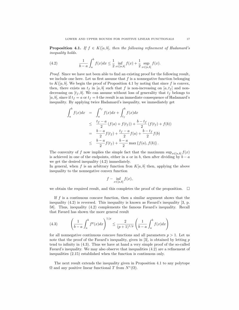
Proposition 4.1. If f ∈ K([a, b], then the following refinement of Hadamard’sinequality holds.

(4.2)1

b− a

∫ b

a

f(x)dx ≤ 1

2inf

x∈[a,b]f(x) +

1

2supx∈[a,b]

f(x).

Proof. Since we have not been able to find an existing proof for the following result,we include one here. Let us first assume that f is a nonnegative function belongingto K([a, b]. We begin the proof of Proposition 4.1 by noting that since f is convex,then, there exists an tf in [a, b] such that f is non-increasing on [a, tf ] and non-decreasing on [tf , b]. We can assume without loss of generality that tf belongs to]a, b[, since if tf = a or tf = b the result is an immediate consequence of Hadamard’sinequality. By applying twice Hadamard’s inequality, we immediately get∫ b

a

f(x)dx =

∫ tf

a

f(x)dx+

∫ b

tf

f(x)dx

≤ tf − a2

(f(a) + f(tf )) +b− tf

2(f(tf ) + f(b))

=b− a

2f(tf ) +

tf − a2

f(a) +b− tf

2f(b)

≤ b− a2

f(tf ) +b− a

2max f(a), f(b) .

The convexity of f now implies the simple fact that the maximum supx∈[a,b] f(x)is achieved in one of the endpoints, either in a or in b, then after dividing by b− awe get the desired inequality (4.2) immediately.In general, when f is an arbitrary function fron K[a, b] then, applying the aboveinequality to the nonnegative convex function

f − infx∈[a,b]

f(x),

we obtain the required result, and this completes the proof of the proposition.

If f is a continuous concave function, then a similar argument shows that theinequality (4.2) is reversed. This inequality is known as Favard’s inequality [3, p.58]. Thus, inequality (4.2) complements the famous Favard’s inequality. Recallthat Favard has shown the more general result

(4.3)

(1

b− a

∫ b

a

fp(x)dx

)1/p

≤ 2

(p+ 1)1/p

(1

b− a

∫ b

a

f(x)dx

)for all nonnegative continuous concave functions and all parameters p > 1. Let usnote that the proof of the Favard’s inequality, given in [3], is obtained by letting ptend to infinity in (4.3). Thus we have at hand a very simple proof of the so-calledFavard’s inequality. We may also observe that inequalities (4.2) are a refinement ofinequalities (2.15) established when the function is continuous only.

The next result extends the inequality given in Proposition 4.1 to any polytopeΩ and any positive linear functional T from N∗(Ω).

18 ALLAL GUESSAB

Theorem 4.2. Let f ∈ K(Ω) such that f attains its minimum over Ω at xmin.Then the following inequalities are valid:

(4.4) f (cgT (Ω)) ≤ T [f ] ≤ T [φxminn+1 ] inf

x∈Ωf(x) +

(1− T [φxmin

n+1 ])

supx∈Ω

f(x).

Proof. Since f is continuous on Ω, there exist points xmin,xmax ∈ Ω such thatfmin := f(xmin) = infx∈Ω f(x) and fmax := f(xmax) = supx∈Ω f(x). It can easilybe shown that given a convex function over the polytope Ω, then this functionachieves its maximum value at some point among the vertices of Ω. We assumefirst that xmin is an interior point of Ω. Next we apply Theorem 2.4 by choosingy = xmin then the following inequality holds

T [h] ≤n∑i=0

T [φxmini ]h(vi) + T [φxmin

n+1 ]h(xmin),

where h = f − fmin. Then it is clear that, in order to get an upper bounds forT , we need to maximize h(vi) for all vertices of Ω. Thus, since h is a nonnegativefunction on Ω an additional calculation similar to that done above shows that

T [h] ≤ (1− T [φxminn+1 ])h(xmax) + T [φxmin

n+1 ]h(xmin).

Therefore, it follows from the fact that the above inequality becomes an equalityfor constants, we deduce the right-hand side in (4.4) for any continuous convexfunction. Finally, a simple continuity argument shows that equality (4.4) is alsovalid when xmin is a border point of Ω.

Our next result extends the above theorem to any point y that belongs to theinterior of Ω. Indeed, by similar arguments the following more general result canbe proved. For convenience, we reformulate the statement of this result here.

Theorem 4.3. Let y be an arbitrary fixed point in int(Ω). Then, the followinginequalities are valid for any f ∈ K(Ω):

(4.5) f (cgT (Ω)) ≤ T [f ] ≤ T [φyn+1]f(y) +

(1− T [φ

yn+1]

)supx∈Ω

f(x).

The reader may observe that the bounds derived in Theorem 4.2 and 4.3 are al-ways better than those given in (2.15), where we have assumed only the continuityof the functions involved.

Multidimensional integral version: our general upper bound for the integral func-tional setting is not different from that in the one dimension. Indeed, we have thefollowing multivariate version of Favard’s inequality as a corollary to the abovetheorem:

Corollary 4.4. For every convex function belonging to K(Ω) the following inequal-ities are valid:

(4.6) f

(∫Ωxdx

vol(Ω)

)≤∫

Ωf(x)dx

vol(Ω)≤ 1

d+ 1infx∈Ω

f(x) +d

d+ 1supx∈Ω

f(x).

Proof. Just apply the integral identity (2.18) proved in Lemma 2.3.

An interesting aspect of this form is that, in the integral situation, the coefficientT [φxmin

n+1 ] is independent of the point xmin and it is a function of d only.


Remark 4.5. Note that if the function f in Theorems 4.2, 4.3 and Corollary 4.4is concave, then inequalities (4.4), (4.5) and (4.6) hold true, except in these caseseach of these inequalities is reversed (with the order of the sup and inf reversed).

We end this section with a question which is concerned with a possible extensionof Theorem 4.2 and its Corollary 4.4. We may naturally ask whether inequalitiesin (4.4) and (4.6) hold for any compact convex set Ω ⊂ Rd with positive measure.

The answer is no. Indeed, this result can be immediately derived from thefollowing general statement:

Theorem 4.6. Let T ∈ N∗(Ω), where Ω is a compact convex subset of Rd withpositive measure. Assume that there are (m + 1) points x0, . . . ,xm ∈ Ω, and realnumbers a0, . . . , am, such such that, for every f ∈ K(Ω), we have

(4.7) T [f ] ≤ R[f ] :=

m∑i= 0

aif(xi).

Then Ω must be a polytope.

Proof. Let Ω∗ be the convex hull of x0, . . . ,xm. Let us assume to the contrarythat there exists a point, say x∗, which is an element of Ω, but does not belongto Ω∗. We will exhibit a function from K(Ω) for which inequality (4.7) does nothold. Indeed, due to the separation Theorem for closed convex sets (see, e.g., [20,p. 65, Theorem 2.4.1]), there exists an affine function h such that h(x∗) = 1 and his strictly negative on Ω∗. Set

h(x) = max h(x), 0 ,∀x ∈ Ω.

Note that h is a nonnegative function belonging to K(Ω), since it is the maximumof two convex functions. It also vanishes on Ω∗ and takes the value 1 at x∗. We cantherefore conclude, in view of the continuity of h, that there exists a neighbor Uof x∗ such that h is positive. Because T is assumed strictly positive, we then haveT [h] > 0. But, R[h] = 0, this contradicts (4.7) and so Ω must be equal the convexhull of the points x0, . . . ,xm. Thus we can conclude that Ω is a polytope.

This justifies why we have limited our analysis to the case of polytope domains.Finally, we should remark that if Ω is a polytope, then Theorem 2.4 tells us that,every T ∈ N∗(Ω) is dominated in K(Ω) by some functional of the form givenin (4.7). Thus, domination property (4.7) characterizes the polytopes among thecompact convex subsets of Rd.

5. An improvement of the lower and upper bounds and errorestimates

Assume given lower and upper bounds in K(Ω) to a given positive linear func-tional. In the case when f is smooth, this section answers the following question:

• How to properly derive a procedure to be able to generate ‘much better’ lowerand upper bounds than those derived in Section 2 ?

In this situation, this section also establishes a general result concerning errorestimates. More precisely, for smooth (nonconvex) twice continuously differentiable

20 ALLAL GUESSAB

functions, the first part of this section improves both the lower and upper boundsgiven in Theorem 2.4 for any T ∈ N∗(Ω). Our inequalities can be seen as an exten-sion of Hadamard-Favard inequalities for nonconvex functions.In order to present the essentials of the technique, we need some additional neces-sary background and notation.By Sd we denote the set of all d × d symmetric matrices in R. Let A ∈ Sd, andβi[A], i = 1, . . . , d, the (real) eigenvalues of A, we define

βmin[A] := min1≤i≤d

βi[A] = min‖y‖=1

〈Ay,y〉 .

We say A ∈ Sd is positive semidefinite if 〈Ay,y〉 ≥ 0, for every y ∈ Rd. The set ofpositive semidefinite symmetric matrices (all eigenvalues ≥ 0) is denoted by S+

d .By D2f(x), we mean the d × d matrix whose entries are the second-order partialderivatives of f at x. It is well known that when f is a C2(Ω)-function, its convexityis characterized by the fact that for all x ∈ Ω, D2f(x) ∈ S+

d (see e.g. [18]). Forevery x ∈ Ω, the Hessian matrix D2f(x), as real-valued and symmetric matrix, hasreal-valued eigenvalues. Therefore, for every function f in C2(Ω), we may define

λmin[f ] := infx∈Ω

βmin[D2f(x)].

Now, let f be any C2(Ω)−function and set

(5.1) g := f − λmin[f ]

2‖.‖2 ,

(‖.‖2 denotes the Euclidean norm on Rd.) The Hessian matrix of g is

D2g(x) = D2f(x)− λmin[f ]Id,

where Id denotes the d×d identity matrix. Therefore, for y ∈ Rd such that ‖y‖ = 1,we have ⟨

y, D2g(x)(y)⟩

=⟨y, D2f(x)(y)

⟩− λmin[f ].

It is clear from the definition of λmin[f ] that, for every x ∈ Ω, the right-hand termin the above equation is nonnegative. This means that the Hessian matrix of g ispositive semidefinite for all x of the set Ω, and consequently g is convex.Hence, an arbitrary nonconvex twice continuously differentiable function is made

convex after adding to it the quadratic −λmin[f ]2 ‖.‖2 .

Note that λmin[f ] is not necessarily zero if f is convex over Ω. On the other hand,if λmin[f ] ≥ then f is convex over Ω.Let R ( resp. L) be a lower bound (resp. an upper bound) of T on K(Ω), in thesense

(5.2) L[g] ≤ T [g] ≤ R[g],

for all convex functions g ∈ C(Ω). Define

R+[‖.‖2] = R[‖.‖2]− T [‖.‖2],

and

L−[‖.‖2] = T [‖.‖2]− L[‖.‖2].

Note that R+[‖.‖2] and L−[‖.‖2] are nonnegative.


With this notation, the next result shows that, under some regularity assump-tions about the function f , there exist better bounds than those defined in (5.2).More precisely we have:

Theorem 5.1. Let R and L be an upper bound (resp. a lower bound) of T onK(Ω). Then the following bounds hold for every function from C2(Ω):

(5.3) L[f ] +λmin[f ]

2L−[‖.‖2] ≤ T [f ] ≤ R[f ]− λmin[f ]

2R+[‖.‖2].

Proof. In fact, under the present assumption about the function f, it is evidentthat the auxiliary function

g := f − λmin[f ]

2‖.‖2

is convex. Hence we can apply the inequality (5.2) to g and rearranging terms leadsto the required inequality.

We now turn to the error estimates for the approximation of a functional T ∈N∗(Ω) by any lower or upper bounds on K(Ω). The following result characterizesthe error estimates in approximation by functionals of this type.

Proposition 5.2. Let A : Ck(Ω) → R, where k ∈ 0, 1, be a normalized linearfunctional and let σ ∈ −1, 1. The following statements are equivalent:

(i) For every f ∈ C2(Ω), we have

|T [f ]−A[f ]| ≤ σ(T [‖.‖2]−A[‖.‖2]

) ∣∣D2f∣∣

2.

Equality is attained for all functions of the form f(x) := a(x) + c, wherec ∈ R and a is any affine function.

(ii) For every convex function f ∈ C2(Ω), we have

σ (T [f ]−A[f ]) ≥ 0.

Proof. The proof is an immediate consequence of [8, Proposition 2.1].

References

[1] Brenner J. L. , Alzer H., Integral inequalities for concave functions with applications to special

functions, Proc. of the Royal Soc. of Edinburgh 118A, 173–192, 1991.

[2] Chen L., Xu J., Optimal Delaunay triangulations, J. Comput. Math. 22, 299–308, 2004.[3] Favard J., Sur les valeurs moyennes, Bull. Sci. Math. (2) 57, 54–64,1933.[4] Farin, G., Curves and Surfaces for Computer Aided Geometric Design, Academic Press, San

Diego, (1993)[5] Fuglede B., Continuous selection in a convexity theorem of Minkowski,. Expo. Math. 4, 163-

178, 1986.[6] George P.-L., Borouchaki H., Delaunay Triangulation and Meshing: Application to Finite

Elements (Translation from French), Editions Hermes, Paris, 1998.[7] Guessab A., Nouisser O., Pecaric J., A multivariate extension of an inequality of Brenner-

Alzer, Archiv der Mathematik, Volume 98, Number 3, 277–287, 2012.

[8] Guessab A., Nouisser O., Schmeisser G., A definiteness theory for cubature formulae of ordertwo, Constr. Approx. 24 (2006), 263–288.

[9] Guessab A., Schmeisser G., Negative definite cubature formulae, extremality and Delaunay

triangulation, Constr. Approx., Volume 31, 95-113, 2010.[10] Guessab A., Schmeisser G., Construction of positive definite cubature formulae and approx-

imation of functions via Voronoi tessellations, Adv Comput Math, 32, 25-41, 2010.[11] Guessab A., Schmeisser G., A definiteness theory for cubature formulae of order two, Constr.

Approx., 24, 263-288, 2006.

22 ALLAL GUESSAB

[12] Guessab A., Schmeisser G., Sharp integral inequalities of the Hermite-Hadamard type, J.

Approx. Theory, 115, No.2, 260-288, 2002.

[13] Guessab A., Schmeisser G., Convexity results and sharp error estimates in approximate mul-tivariate integration, Math. Comp. 73 (2004), 1365–1384.

[14] Hammer, P. C., The midpoint method of numerical integration. Math. Mag. 31 (1958), 193–

195.[15] Kalman J. A., Continuity and convexity of projections and barycentric coordinates in convex

polyhedra, Pacific J. of Math., II, 1017-1022 (1961).

[16] Mcshane E. J., Jensen?s inequality, Bull. Amer. Math. Soc., 43 (1937), 521–527.[17] Pecaric J., F. Proschan, Y.L. Tong, Convex functions, partial orderings and statistical appli-

cations, Academic Press, New York, 1992

[18] Schneider R., Convex bodies: the Brunn-Minkowski theory. Encyclopedia of Mathematicsand its Applications, 44. Cambridge University Press, Cambridge (1993).

[19] J. Warren, Barycentric coordinates for convex polytopes, Adv. Comput. Math. 6, 97-108,1996.

[20] R. Webster, Convexity, Oxford University Press, Oxford, 1994.

January 5, 2013

Laboratoire de Mathematiques et de leurs Applications, UMR CNRS 4152, Universitede Pau et des Pays de l’Adour, 64000 Pau, France

E-mail address: [email protected]

lower and upper bounds for positive linear functionals

Documents