ls-dyna modeling guideline - v12-1 - aerospace working group

LS-DYNA Aerospace Working Group

Modeling Guidelines Document

Version 12-1 dated June 1, 2012

Table of Contents

1.0 Introduction

2.0 General Modeling Guidelines

2.1 Elements

2.1.1 Solid Elements

2.1.2 Shell Elements

2.2 Hourglass Control

2.3 Contact

2.4 Constraints and Rigid Bodies

2.5 Control parameters

2.6 Meshing

2.6.1 Lagrange Elements

2.6.2 ALE/Euler Elements

2.7 Post-Processing

2.8 Modeling Guidelines Checklist

2.9 Units

3.0 Material Modeling Guidelines

3.1 Elasto-Plastic

3.2 Low Density Foam

3.3 Thermoplastics

3.3.1 Using MAT_024

3.3.2 Using MAT_187

3.4 Ice

3.5 Composites

3.5.1 Composites Delamination

3.5.1.1 Cohesive Zone

3.5.1.2 Constitutive Model

3.5.1.3 Mixed Modes

3.5.1.4 Practical Solution with Coarse Mesh

3.6 Material Test Interaction

3.6.1 Model Creation

3.6.2 Model Validation and Verification

3.7 Material Model Failure Calibration

3.8 Equations of State

3.8.1 Perfect Gases

3.8.2 Liquids

3.9 Fluids

3.9.1 Air

3.9.2 Water

3.10 Fabrics

4.0 ALE Modeling Guidelines

4.1 Introduction

4.1.1 Lagrangian

4.1.2 Eulerian

4.1.3 ALE

4.1.4 Mesh Smoothing

4.1.5 Fluid-Structure Interaction (FSI)

4.1.6 Limitations

4.2 ALE Element Formulation

4.3 Meshing

4.4 Coupling Lagrangian Surfaces to ALE Materials

4.5 Modeling Inflow and Outflow Conditions

4.6 Pressure Initialization in ALE Materials

4.7 Post-Processing

4.8 Troubleshooting

5.0 Aerospace Applications

5.1 Stress Initialization for Spinning Bodies

5.1.1 Implicit Pre-Stress Static Solution

5.1.2 Explicit Transient Rotation

5.1.3 Stable Solution Check

5.1.4 Implicit Static Unload

5.2 Bird-Strike

5.2.1 Bird Material Model

5.2.2 Analysis Formulations

5.2.2.1 Lagrange

5.3 Fuel Slosh

5.4 Disk Burst Containment

5.5 Debris Impact

5.6 Ice Slab and Hail Ingestion

5.7 Fan Blade-Off

5.7.1 FAA Requirements under CFR 33.94

5.7.1.1 Current Process of Engine Certification to Demonstrate Compliance with CFR 33.94

5.7.1.2 Role of Analysis in Current Certification Process and Future Direction

5.7.2 Physics of Blade-Off Event and Analytical Considerations in Modeling

5.7.3

Current State of FBO Simulation & Historical Perspective of Nonlinear Analytical Dynamics

Advances

5.7.4 Modeling Considerations

5.7.4.1 Process of Developing a Validated LS-DYNA Model

5.7.4.2 Types of Analyses in LS-DYNA

5.7.4.3 Fan Blade Modeling Considerations

5.7.4.4 Fan Case Modeling Considerations

5.7.4.4.1 Partial Sector Analysis for Containment Evaluation

5.7.4.4.2 Soft-Wall Containment (Kevlar) LS-DYNA Modeling Considerations

5.7.4.4.3 Hard-Wall Containment Modeling and Fragmentation of the Release

5.7.4.5 Combined Dynamic Response of the Engine due to Impact and Unbalance Forces

5.7.4.5.1 Details of the Rotor and Bearing Modeling

5.7.4.5.2 Details of the Engine Mounts and Supporting Structure

5.7.4.5.3 Details of Additional Non-Rotating Engine Structure and Attached Accessories

5.7.4.5.4 Analysis Considerations for Fire Evaluation and Limitations of Explicit

5.7.5 Quality and Validity of LS-DYNA Analytical Results

5.7.6 Transient Dynamic Response of the Rotor after Blade-Loss

5.7.6.1 Bearing Loads – Effect of Bearing Support Fusing

5.7.6.2 Fan Rotor Orbit

5.7.6.3 Dynamic Loads due to Tips of the Fan Blades Rubbing Against the Case

5.7.6.4 Dynamic Response of Engine Access

5.7.6.5 Rubbing Between Concentric Rotors

5.7.7 Windmilling and Rotor Stability

6.0 References

7.0 Revision History

1.0 Introduction

A goal of the LS-DYNA Aerospace Working Group is to produce an evolving set of

guidelines for modeling dynamic aerospace-type problems with LS-DYNA®. These

guidelines are not meant to limit analysts in their approach to a specific problem, but

instead are intended to assist them in getting started and to serve as a basis of

comparison when evaluating results from new or unproven modeling techniques.

The current version of this document resides online at awg.lstc.com. All working group

members are encouraged to critique the document and to submit modifications and/or

additions via email to the document editor. The document is, thus, not intended to be

the product of one individual or company, but rather a collective product of the

Aerospace Working Group.

2.0 General Modeling Guidelines

The modeling guidelines in this section are of a general nature and apply not only to

aerospace events, but also to other dynamic events, e.g., automobile crash.

In this document, LS-DYNA input parameter names are written in uppercase letters, e.g.,

ELFORM; and LS-DYNA keyword commands are also written in uppercase, but are

preceded by an asterisk, e.g., *SECTION_SHELL. Complete descriptions of LS-DYNA

keyword commands and the associated input parameters are given in the current

edition of the LS-DYNA Users Manual.

2.1 Elements

Elements types in LS-DYNA include solids, shells, thick shells, beams, springs/dampers,

and discrete mass/inertia elements. Only solids and shells are discussed herein, as

these are the two predominant element types used in aerospace impact simulations.

Invariant node numbering should be turned on via INN in *CONTROL_ACCURACY for

shells (INN=2 or 4), solids of anisotropic material (INN=3 or 4), and solids of any material

when hourglass formulation 6 is invoked (INN=3 or 4). This is especially important for

shells of anisotropic materials or when elements distort due to shearing or hourglassing.

By making the element rotation calculation independent of the order of the nodes,

invariant node numbering makes the results insensitive to the element connectivity.

2.1.1 Solid Elements

Solid elements are able to capture fully three-dimensional states of stress and are

generally used to model thick parts or continua. In contrast, parts that are relatively

thin in one direction are generally modeled with shell elements (Section 2.1.2). To

model a thin part with solids can be expensive since (a) the smallest dimension of a solid

will control its time step, and (b) generally two or more solid elements through the

thickness are required to produce an accurate response. When the analysis objective is

to duplicate a fracture observed in test, significantly more elements will likely be needed.

An exception to (a) would be modeling a cohesive layer via *MAT_COHESIVE and solid

element formulation 19 or 20 (ELFORM=19 or 20 in *SECTION_SOLID). Exceptions to (b)

would include:

• Using ELFORM=1 (*SECTION_SOLID) and hourglass type 6 with an hourglass

coefficient of 1.0 (Section 2.2) will provide proper bending stiffness of an elastic

component modeled with only one element through the thickness. For

nonlinear materials, if ELFORM 1 solids are used, meshing with at least three

elements through the thickness of a component is recommended soas to allow

for a nonlinear distribution of stress through the thickness.

• Using 2x2x2 integration via ELFORM 2 (*SECTION_SOLID) may allow a coarser

mesh to be used, but this element formulation is prone to shear locking if the

element aspect ratio is poor.

When using solid elements, hexahedrons are preferred. If tetrahedrons or

pentahedrons are interspersed with hexahedrons in any single part, set ESORT=1 in

*CONTROL_SOLID. This will automatically assign ELFORM 15 to otherwise degenerate

pentahedrons and ELFORM 10 to otherwise degenerate tetrahedrons. If a solid part is

comprised entirely of pentahedrons (not recommended), set ELFORM to 15 for that part

or else set ESORT=1. If a part is comprised entirely of tetrahedrons, there are several

tetrahedral formulations to choose from, each with various pros and cons. Any of the

following formulations would be preferable to using degenerate, ELFORM 1

tetrahedrons:

• ELFORM 10: 1 point tetrahedron with 4 nodes that is prone to volumetric locking

(overly stiff behavior) in incompressible regimes, e.g., as in plasticity. Generally,

this is acceptable for foams.

• ELFORM 4: 4 or 5 point, selectively-reduced quadratic tetrahedron with 4 nodes

and nodal rotations. This may give spurious results in applications involving

contact.

• ELFORM 13: 1 point nodal pressure tetrahedron developed for bulk metal

forming. This is always used in a part in which 3D r-adaptivity is invoked.

• ELFORM 16: 4 or 5 point, 10-noded tetrahedron. The time step of a 10-noded

tetrahedron will be half that of a 4-noded tetrahedron. The nodal weighting

factors are not proportionately correct.

• ELFORM 17 (v. 971 only): 10-noded tetrahedron with equal weighting factors for

all nodes. This is intended as an improvement over ELFORM 16.

Even with this array of tetrahedral formulations, hexahedrons with ELFORM 1 are

generally preferred over tetrahedrons for reasons of computational efficiency and

because hexahedron elements with ELFORM 1 are known to give reliable response

under a wider range of conditions provided that suitable hourglass control is used.

2.1.2 Shell Elements

Shell elements are plane stress elements (zz = 0) with a variable number of integration

points through the thickness. Shells are useful for modeling thin components, since

than one element through the thickness is not required and thickness does not factor

into the time step calculation. When the material is nonlinear, a minimum of three

through-thickness integration points is recommended so that a nonlinear stress

distribution can be calculated. Two integration points through the thickness is sufficient

for elastic materials.

For isotropic, homogeneous shells, the shear correction factor SHRF in *SECTION_SHELL

should be set to the theoretically correct value of 0.833. Note that the default value of

SHRF is 1.0.

In impact analyses, consideration of shell thinning is generally unimportant and may

make the solution more prone to instability. It is thus recommended that the shell

thinning option not be invoked, i.e., ISTUPD in *CONTROL_SHELL should be left to its

default value of 0. Setting ISTUPD to 1 and, thus, including the effects of shell thinning

may have the undesired effect of causing a numerical instability leading to an abnormal

termination of the analysis. If the user deems it necessary to include the effects of shell

thinning for a subset of parts, version 971 includes the parameter PSSTUPD in

*CONTROL_SHELL which allows control over which shell parts include the effects of shell

thinning. This allows the user to be selective in specifying where shell thinning is to be

considered. Furthermore, version 971 includes a new thinning option for shells

comprised of isotropic, plastic material. The new option is invoked by setting ISTUPD to

4 and should be more stable than ISTUPD = 1, since the elastic strains are neglected in

the thickness update.

For shell structures that undergo dynamic buckling or predominantly compressive

modes of deformation, stability may be enhanced by invoking bulk viscosity for shell

formulations 2, 10, and 16. This is done by setting TYPE to -1 or -2 in

*CONTROL_BULK_VISCOSITY. TYPE = -2 is the same as TYPE = -1 except that energy

associated with the bulk viscosity is included in the energy balance (recommended).

When meshing with shell elements, bear in mind that quadrilateral elements are

preferred over triangular elements. Triangular elements do not have hourglass modes,

however, they can behave in too stiff a manner. If triangular elements are present, and,

particularly if they are interspersed with quad elements in any given part, set ESORT=1

in *CONTROL_SHELL. Quadrilateral shells that are initially warped or that become

warped due to deformation can be a problem unless certain options are invoked. The

parameter to invoke appropriate warping stiffness depends on the shell formulation

chosen:

Under-integrated shell formulations (can develop hourglass modes)

• ELFORM 1: Set IRNXX to -2 in * CONTROL_SHELL.

• ELFORM 2: Set BWC to 1 and PROJ to 1 in * CONTROL_SHELL.

Fully-integrated shell formulations

• ELFORM 6,7: Set IRNXX to -2 in * CONTROL_SHELL.

• ELFORM 16: Set hourglass type IHQ to 8.

2.2 Hourglass Control

With the exception of triangular shells and tetrahedral solids, any under-integrated shell

or solid formulation will undergo nonphysical modes of deformation called hourglass

modes. It is important to inhibit these hourglass modes by internally calculating and

applying counteracting forces, but in a prudent manner so as to not significantly

dissipate energy. The undesirable dissipated energy or ‘hourglass energy’ is simply the

work done by the ‘hourglass forces’ that are applied to counteract the hourglass modes.

Though hourglass modes and hourglass energy are a nonissue for fully-integrated

element formulations, there are good reasons for using under-integrated element

formulations. Chief among these reasons is the relatively low cost and the robustness of

under-integrated element formulations.

The hourglass type IHQ and hourglass coefficient QM can be set for a particular part by

defining the first three parameters in *HOURGLASS and then setting the hourglass

identification number HGID in *PART to HGID in * HOURGLASS. The * HOURGLASS

command can appear any number of times, i.e., more than one set of hourglass

parameters can be established with each set being identified by a unique HGID. If no

HGID is specified in *PART, the hourglass type and coefficient for the part is taken from

IHQ and QH defined in *CONTROL_ HOURGLASS and, if *CONTROL_ HOURGLASS is not

defined, the hourglass type and coefficient default to 1 and 0.1, respectively.

Hourglass type 1 is the most inexpensive hourglass control and it may give acceptable

results, however, other hourglass formulations are generally more effective. The usual

gage for evaluating the effectiveness of the hourglass control is the ratio of hourglass

energy to peak internal energy. The target is to achieve a ratio of 0.1 for the entire

model and also, ideally, for each part. To make this assessment, set HGE to 2 in

*CONTROL_ENERGY and write glstat and matsum files by including *DATABASE_GLSTAT

and *DATABASE_MATSUM commands in the input deck.

For impacts of low to moderate velocity (granted, an indefinite description), the

recommendation for relatively stiff materials, e.g., metals, composites, and polymers, is

to use hourglass formulation 4 with an hourglass coefficient of 0.05 or less. Type 4

hourglass control is stiffness-based and, thus, the hourglass forces are proportional to

the displacements contributing to the hourglass modes. These forces thus counteract

the accumulated hourglass deformation. There is an inherent stiffening effect of a

stiffness-based hourglass control; hence, the recommended reduction in the hourglass

coefficient so as to reduce this effect.

For relatively stiff materials at moderate to high impact velocities, a viscous hourglass

formulation (types 2 or 3 are preferred over type 1) with the default hourglass

coefficient (0.1) recommended. The same recommendation also applies to relatively

soft materials, e.g., foams and rubbers, regardless of the impact velocity. In a viscous

hourglass formulation, the hourglass forces are proportional to the velocities

contributing to the hourglass modes. These forces thus counteract only the incremental

hourglass deformation. In contrast to the stiffness-based hourglass control, there is no

unwanted side effect of artificial stiffening.

A suggested alternative for ELFORM 1 solid elements, particularly for soft materials, is

hourglass formulation 6.

When modeling fluids, whether as Lagrangian (ELFORM 1) or as ALE (ELFORM 11,12),

hourglass type 1 with a significantly reduced hourglass coefficient, e.g., 0.001 or less, is

recommended.

2.3 Contact

A complete overview of contact modeling in LS-DYNA is beyond the scope of this

document, however, guidelines for contact modeling which are applicable to impact

analysis are presented herein. Broader overviews and examples of contact modeling

are available in the tutorials section of the working group web page, and online at

http://www.dynamore.info/Support/tutorial/users.guide/contact.modeling

http://www.dynamore.info/Support/tutorial/contact.modeling

Contact modeling guidelines and recommendations are:

• Use automatic contacts, e.g., *CONTACT_AUTOMATIC_SINGLE_SURFACE, to

define contact of parts which are not tied or merged together.

o When generating the mesh for shells and beams, bear in mind that

automatic contacts always offset the contact surfaces from the shell

midplane by half the ‘contact thickness’. Furthermore, the contact

surface wraps around the exterior edges of shells so that the contact

surface is smooth and continuous. The default contact thickness is equal

to the shell thickness, but it can be modified via SST and MST on Card 3 of

*CONTACT or, if automatic_single_surface contact is used, via OPTT in

*PART_CONTACT. Contact thickness should NOT be set to a very small

value. On the contrary, it is often beneficial to set the contact thickness

to a value greater than the shell thickness (> 1 mm) if the shell thickness

is extremely small.

o Do NOT define redundant contacts. In other words, contact interaction

between any two segments or between any node and a segment should

be handled by one and only one *CONTACT definition.

o Use *CONTACT_AUTOMATIC_GENERAL to handle beam-to-beam contact.

This contact type also handles most other interactions, but it is not

generally recommended owing to its added expense. SOFT may be set to

1 for this contact type if the contact behavior appears too soft.

o Use an eroding contact type, e.g.,

*CONTACT_ERODING_SINGLE_SURFACE, if one or more of the parts

included in the contact definition include failure criteria such that

elements can be deleted as the solution progresses. Eroding contact

updates the contact surface to account for the loss of elements.

o Set SOFT=2 on Optional Card A of *CONTACT if one of the following

contacts is used: automatic_surface_to_surface,

automatic_single_surface, eroding_single_surface. Furthermore, set

DEPTH = 5 on Optional Card A to handle shell edge-to-edge contact.

• Tied or tiebreak contacts can be used to join or ‘glue’ parts or surfaces together

in cases where merging nodes is not practical or possible.

o To tie together surfaces comprised of deformable solid elements, use

*CONTACT_TIED_SURFACE_TO_SURFACE. If one of the surfaces is or is

part of a rigid body, use *CONSTRAINED_EXTRA_NODES to include the

nodes of the deformable surface in that rigid body.

o To tie a deformable shell surface or shell edge to another deformable

shell surface, use *CONTACT_TIED_SHELL_EDGE_TO_SURFACE if there is

no gap between the slave and master surface. If there is a gap that needs

to be retained, use

*CONTACT_TIED_SHELL_EDGE_TO_SURFACE_BEAM_OFFSET (this works

for deformable and rigid surfaces).

o To tie two rigid bodies together, merge them using

*CONSTRAINED_RIGID_BODIES.

o To tie together surfaces in a nonpermanent fashion, a failure criterion to

release the tied condition must be specified in a ‘tiebreak’ contact.

Tiebreak contacts are penalty-based which means they can be used with

both deformable and rigid bodies. In its simplest form (OPTION=2),

*CONTACT_AUTOMATIC_SURFACE_TO_SURFACE_TIEBREAK offers a

tension and shear stress-based failure criterion and reverts to an

automatic_surface_to_surface subsequent to failure. Please refer to the

LS-DYNA User’s Manual for a description of other values of OPTION that

invoke other tiebreak treatments.

2.4 Constraints and Rigid Bodies

Avoid the use of *CONSTRAINED_NODE_SET unless nodes in the node set are coincident.

To rigidly connect two or more deformable, noncoincident nodes, use

*CONSTRAINED_NODAL_RIGID_BODY instead of *CONSTRAINED_NODE_SET so that

nonphysical resistance to rotation is not imposed.

A rigid body can be defined in LS-DYNA in several ways:

• A part that references *MAT_RIGID is a rigid body.

• A set of nodes referenced by *CONSTRAINED_NODAL_RIGID_BODY forms a rigid

body.

• A node or set of nodes referenced by *CONSTRAINED_EXTRA_NODES is added to

or becomes a rigid body.

Rigid bodies are subject to certain rules of modeling to which deformable bodies are not.

For example:

• With few exceptions, *CONSTRAINED_OPTION cannot be applied to any element

or part that is rigid or to any node that is included in a rigid body. The exceptions

are * CONSTRAINED_RIGID_BODIES, * CONSTRAINED_JOINT, and *

CONSTRAINED_LAGRANGE_IN_SOLID (if penalty-based coupling is used).

• Constraint-based contact algorithms, predominately used in LS-DYNA in tied (not

tiebreak) contact types, cannot be used on rigid bodies.

• Prescribed motion cannot be applied to more than one node of a rigid body. The

preferred method of prescribing motion to a rigid body is via

*BOUNDARY_PRESCRIBED_MOTION_RIGID in which the motion is defined with

respect to the center-of-mass of the rigid body.

• Though nodal single-point-constraints (*BOUNDARY_SPC) on nodes of rigid

bodies will internally be converted by LS-DYNA into an equivalent set of

constraints on the rigid body’s center-of-mass, the preferred method of

constraining rigid body motion is via Card 2 of *MAT_RIGID, or if the rigid body is

defined as a nodal rigid body, via *CONSTRAINED_NODAL_RIGID_BODY_SPC.

*BOUNDARY_PRESCRIBED_MOTION_RIGID would be another acceptable means

of constraining a rigid body (velocity or displacement could be prescribed as

zero).

The mesh of rigid bodies should generally be no coarser than that of a deformable body,

unless the rigid body’s motion is fully constrained and/or prescribed, or unless the mass

properties are specified directly via *PART_INERTIA. Because mass is lumped at the

nodes, a coarse mesh will often give highly inaccurate inertia values.

Be aware that all elements having the same part ID, if comprised of *MAT_RIGID, are

grouped together as a single rigid body even if the elements are separated by space or

elements with a different part ID. If the intent is for each spatially distinct group of rigid

elements to behave independently, each group should be given a different part ID.

If initial velocity is specified for a rigid body, confirm that the initial velocity is correct by

displaying velocity vectors from state 1 of the d3plot database. If the initial velocity

profile is not exactly what was expected, be aware that there is a hierarchy to the

commands controlling initial velocity. For rigid bodies, *PART_INERTIA is at the top of

that hierarchy, followed by *INITIAL_VELOCITY_RIGID. If *

INITIAL_VELOCITY_GENERATION is used to assign initial velocity to a rigid body, PHASE

must be set to 0. It is acceptable to have two separate *

INITIAL_VELOCITY_GENERATION commands: one with PHASE=0 for rigid bodies and one

with PHASE=1 (if dynamic relaxation is included) for deformable bodies.

2.5 Control Parameters

When running a shared memory parallel (SMP) executable, set the consistency flag

CONST to 1 in *CONTROL_PARALLEL. This can also be accomplished on the execution

line by setting “ncpu” to a negative number, e.g., “ncpu=-2” would run the job on 2

processors with the consistency flag turned on.

2.6 Meshing

2.6.1 Lagrange Elements

Listed below, in no particular order, are factors to be taken into consideration when

deciding on Lagrangian mesh density.

Model Geometry

The finite element mesh density determines how well or how accurately the meshed

geometry represents the actual geometry. As the model deforms, the geometry

changes, e.g, a flat plate can buckle into a folded, accordion shape. The mesh density

determines how well the deformed shape can be resolved. Using the example of shell

buckling again, we don't want unnatural kinks too develop as a result of a too-coarse

mesh. Folds that develop as a result of buckling should appear smooth.

Element Formulation

Mesh refinement should be higher (smaller elements) for lower order or under-

integrated elements than for higher order or fully integrated elements. Bear in mind

that a finer mesh of under-integrated elements is preferred for explicit simulations even

though hourglass energy must be monitored. Fully integrated elements are prone to

locking behavior, are more apt to develop negative volumes (solids), and are much more

expensive than under-integrated elements.

Stress Gradients

The shape of the part being modeled, as well as loads and boundary conditions, affect

the local gradients of stress and deformation. To accuracy predict stress where

gradients are high requires a finer mesh density as compared to regions where gradients

are not so steep.

Accuracy of Through-Thickness Stress Distribution

Linear materials, e.g., *MAT_ELASTIC, require only two integration points through the

thickness of a part in order to give the correct stiffness. Nonlinear materials, e.g., any

plasticity model, will need more than two integration points through the thickness of a

part if the material has entered the nonlinear regime. For thick parts, five or more

integration points will improve accuracy. When modeling with under-integrated solids

(ELFORM=1), each element has only one integration point so if, for example, three

integration points are desired through the thickness, this is accomplished by meshing

with three solid elements through the thickness. To get accurate surface bending

stresses with under-integrated elements, the mesh should be biased to the inner and

outer surfaces.

Analysis Objective(s) and Mesh Size

The appropriate mesh refinement depends on the objective(s) of the particular analysis

under consideration:

If the objective is to quantify global displacement of a structure in which parts may yield

but do not fail, a relatively coarse mesh might suffice.

If the objective is to accurately capture the shape of parts that buckle and fold during

the simulation, there is a minimum mesh density that is required. To determine if the

mesh has sufficient refinement, increase the mesh density and re-run the analysis. If

the buckling behavior is unchanged, then the solution has converged and the mesh is

adequate. (This assessment of mesh convergence can be applied to failure cases by

running test cases in the plastic region to assess the mesh quality prior to running failure

cases.)

If the objective is to evaluate the potential for failure in a particular component under

extreme loading, a fine mesh of that component is likely required to predict the failure

mode. Complicating matters is that, in the case where a failure criterion is invoked for a

material, the simulation may not 'converge' to a unique solution as the mesh is refined.

In such a situation, the parameter(s) controlling material failure are generally

established through calibration with test data using a particular mesh density. Care

should be taken to insure that the calibration mesh size is the same mesh size in the

component being analyzed. If the mesh size changes, it's likely the failure parameter(s)

must also change in order to get good agreement with the test data. Failure models

that have regularization, however, account for nominal changes from the calibration

mesh size to the actual component mesh size. Significant differences in size or aspect

ratio can, however, affect the results.

Mass Distribution

LS-DYNA lumps all mass at the nodes. Mass properties, including the inertia tensor, are

calculated based on this mass-lumped-to-nodes arrangement. The coarser the mesh is,

the less accurate the mass properties are, especially the terms in the inertia tensor. An

inaccurate inertia tensor will result in inaccurate prediction of body rotation.

Hourglassing

When modeling with under-integrated element formulations, nonphysical hourglass

modes of deformation and hourglass energy (work done by internal forces applied to

resist hourglass deformation) are of concern. Coarser meshes have a greater tendency

for hourglass modes to be excited and/or larger hourglass energy to develop.

Time and Labor

Whereas an overly fine mesh is acceptable from an accuracy standpoint, overall run

time is adversely affected due to an unnecessarily large number of elements and,

perhaps more importantly, the effect of the element size on time step. Recall that for

explicit analysis, the solution time step is the shortest time it takes a stress wave to

traverse any element. Thus, smaller elements result in a smaller time step. A

compromise must be struck so that the mesh is fine enough to achieve the simulation

objective(s) but not overly fine so as to result in unnecessarily long run times. To

varying degrees, most analysts sacrifice quality of mesh in the interest of time savings,

since quality mesh building tends to be labor intensive. Often, the decision to sacrifice

mesh quality in order to obtain quick results is seen in hindsight as a poor tradeoff, since

it can lead to false or misleading results and a subsequent need to remesh and reanalyze

the model.

Owing to the number of factors which should enter into the decision of how to mesh a

model, it is difficult to formulate a cookbook of guidelines for meshing. In practice,

meshing is largely a matter of engineering judgment based on experience and the

situation at hand. When in doubt, a mesh sensitivity study is recommended. Examples

of mesh sensitivity studies are described below.

In his "Crashworthiness Engineering Crash Notes"[1], Paul Du Bois examines the effect

of mesh density in several case studies, e.g.,

• Buckling of a hat section: "The study shows 16 elements per side to be adequate

in describing the physical behavior with sufficient accuracy; 12 elements per side

gives an approximate solutions.", p. I.17.

• Reduced integration shells and in-plane bending: 10-by-3 and 10-by-4 shell

meshes of ELFORM 2 shells converge. 10-by-2 mesh over-predicts deflection by

20%. 10-by-1 mesh diverges. "The need to accurately represent in-plane

bending stiffness of structures thus leads to the requirement of using a minimum

of 3 under-integrated elements between any 2 [entities] such as kinks, loads,

boundary conditions, connections, etc." Also, "In particular a minimum of 3

under-integrated elements should be used per side of any open or closed

section.", p. 2.34.

• Reduced integration shells and out-of-plane bending: "The conclusion is again

that 3 [under-integrated] elements per side of any open or closed section

represents a minimum condition for meshing since 2 elements will be rather

sensitive to hourglass modes under arbitrary loading.", p. 2.40.

In "A Mesh Refinement Study on the Impact Response of a Shuttle Leading-Edge Panel

Finite Element Simulation"[2], the influence of mesh density of a foam projectile and the

carbon-carbon target panel was studied via a series of LS-DYNA analyses in which only

the mesh densities were varied. This paper provides good insight into the

computational expense of an overly fine mesh and the limitations in accuracy of a

coarse mesh.

Mesh Size Validation

For the case where no failure is involved, validation of the model mesh by means of a

mesh sensitivity study is recommended. Results which do not change significantly after

refining the mesh would give confidence to the analyst that the original, coarser mesh is

sufficient for the purpose of the simulation. Unacceptable dissimilar results likely

indicate that the coarser mesh is not sufficiently refined. Conversely, if the results from

a coarser mesh are similar to those from the original, finer mesh, this would indicate

that the coarser mesh is adequate and would present a more economical alternative for

future analyses. Dissimilar results, however, would provide no indication over the

goodness of the original mesh.

When failure is involved, analysts must balance the failure calibration mesh size with the

actual model mesh size. Mesh refinement of a plastically deformed case is

recommended to determine the mesh size needed for consistent analysis results and, if

necessary, the calibration case may need to be re-run with the model mesh size for

accurate results.

Mesh Adaptivity

When modeling with shell elements in LS-DYNA, h-method adaptivity can be invoked so

that the mesh is automatically and selectively refined during the analysis. To some

extent, this feature may act as a substitute for careful planning and meticulous

construction of an initial mesh that can accurately resolve deformations as they develop.

See *CONTROL_ADAPTIVE in the 971 LS-DYNA Users Manual. This method is not

recommended for impact problems with failure.

Element Shape

For shells, quadrilaterals are preferred over triangles. There is no particular cutoff for

shell-thickness-to-edge-length ratio. Squat shell elements, i.e., shells with a large shell-

thickness-to-edge-length ratio, are often used and do not normally present a problem,

though one should be aware of the possible effect on default contact thickness. In

general, 8-noded thick shell elements (*ELEMENT_TSHELL) will likely be more accurate

than 4-noded shells if the thickness-to-radius-of-curvature of the part being modeled

exceeds 0.1. Connectivity of a tshell element is extremely important because it

determines the through-thickness direction.

For solids, hexahedrons are preferred over tetrahedrons or pentathedrons. Use of

automatic meshing algorithms for volumes is discouraged as these automatic meshers

generate tetrahedral elements which are often of poor shape. The ideal element aspect

ratio of 1:1 (shell quads) or 1:1:1 (solid hexes) is rarely achievable, but nevertheless

should be the goal when constructing a mesh.

2.6.2 ALE/Euler Elements

A uniformly fine mesh is commonly used and is generally recommended when using

solid ELFORM 11 (ALE/Euler multi-material formulation). Sometimes, large pressure

gradients in the material dictate that a finer mesh be used in the high gradient regions

in which case transitions from larger elements to smaller elements should be gradual.

Abrupt changes in mesh refinement should be avoided. If the high pressure gradients

are moving in space, which is often the case, *ALE_REFERENCE_SYSTEM can be used

effectively so that the mesh moves in some prescribed manner so as to follow the

moving material and/or high pressure gradients. The mesh can be made to translate,

rotate, expand, and contract following specific instructions from the user or

automatically based on motion of the materials. A changing mesh is what

fundamentally distinguishes ALE from Eulerian.

Be aware that initially poor element aspect ratios can lead to negative volumes during

the Lagrangian step(s) taken prior to advection. If the appropriateness of a particular

mesh density is in doubt, try increasingly finer ALE mesh resolutions until the solution

converges, i.e., until the solution doesn't change significantly.

The appropriate penalty coupling quadrature (NQUAD in

*CONSTRAINED_LAGRANGE_IN_SOLID) depends on the relative sizes of the Lagrange

and ALE elements. The default NQUAD=2 should work well if the ALE and Lagrange

meshes have approximately the same element size. A larger value of NQUAD may be

necessary if the ALE elements are smaller than the Lagrange elements.

Mesh Size Validation for ALE

All the previous considerations for the Lagrange elements apply to the ALE elements. It

is worth noting that advection generally leads to some degree of non-conservation of

energy (see LS-DYNA 971 Keyword User’s , *CONTROL_ALE, Remark 5). Increasing

mesh refinement may result in better overall energy conservation, a physical and

quantifiable measure under the heading of “total energy / initial energy” in glstat. A

value of 1.0 for this ratio indicates perfect energy conservation. If only the ALE mesh is

refined (as opposed to refining both Lagrangian and ALE meshes), the number of

coupling integration points (NQUAD) should generally be increased.

2.7 Post-Processing Guidelines

Check part masses and/or total mass reported in the d3hsp file.

Animate the plot states and look for nonphysical behavior such as parts passing through

other parts.

Check energies reported in glstat and matsum. This requires use of the

*CONTROL_ENERGY, *DATABASE_GLSTAT, and *DATABASE_MATSUM commands in the

input deck. Things to look for are:

• The energy ratio reported in glstat should not wander far (1 or 2 percent) from

1.0. Momentary deviations, even large ones, are generally okay, especially if

they occur early in the simulation.

• Hourglass energy should be small relative to peak internal energy. A quick visual

check can be made from the glstat data by plotting internal energy and hourglass

energy on the same graph. A more robust check is to do the same thing part-by-

part using the matsum data. In all cases, the rule-of-thumb is that hourglass

energy should be less than 10% of the peak internal energy.

• If contact friction is zero, the contact energy (“sliding energy”) reported in glstat

should be small relative to internal energy. Brief, unsustained spikes in the

contact energy are generally acceptable. If a contact energy problem is evident

from the glstat file and there are multiple contacts defined in the model, it helps

to also have a sleout file (*DATABASE_SLEOUT) in order to pinpoint which

contact(s) require scrutiny.

• If contact friction is nonzero, contact energy will include energy dissipated by

friction and, thus, the value should be positive and not necessarily small.

In order to obtain strain tensor output, set STRFLG=1 in * DATABASE_EXTENT_BINARY.

Logarithmic (true) strains are then available when post-processing.

Shell stresses may be obtained from each through-thickness integration point provided

MAXINT in * DATABASE_EXTENT_BINARY is set to the total number of through-thickness

integration points. The terms “upper” and “lower” used in describing stresses or strains

in shells actually refer to the uppermost and lowermost integration points, respectively,

and not, except in the case of Lobatto integration (INTGRD=1 in *CONTROL_SHELL), the

upper and lower surfaces of the shell.

Stresses of Hughes-Liu (ELFORM 1) beams may be obtained from each cross-section

integration point provided BEAMIP in * DATABASE_ EXTENT_BINARY is set to the total

number of cross-section integration points.

2.8 Modeling Guidelines Checklist

The following lists of questions, not all of which are applicable to each analysis, have

been devised as a modeling guidelines checklist for reference by users.

Mesh Considerations

• Are stress gradients resolved within acceptable precision given the geometry?

• Does the mesh size provide an acceptable time-step given the material properties

(for explicit analyses only)?

• Was a mesh sensitivity study performed on the model or a sub-model?

• Is the mesh fine enough to ensure energy conservation (ALE analyses only)?

• Are element inertias approximated well enough by the mass lumped at the nodes?

• If using under-integrated elements, is hourglass energy small enough or the level of

hourglassing acceptable?

• Are the minimum conditions to provide an accurate in-plane/out-of-plane bending

response satisfied in terms of mesh density?

• Are the minimum conditions to capture buckling satisfied in terms of mesh density?

• Are reasonable aspect ratios for solids and shells being used?

• Are shells thickness-length ratios small enough to provide accurate results?

• Are through-thickness stress distributions being captured correctly?

Mesh Quality Checks

• Do parts meshed with shell elements have enough clearance to account for the shell

thickness (only for *CONTACT_AUTOMATIC_...)?

• Are duplicate elements avoided, i.e., two elements with identical connectivity with

the same set of nodes?

• Are free edges avoided where there should be none (i.e. contiguous elements not

sharing the same set of nodes on one side, thus resulting in invisible “cracks” on the

surface)

Element Choice

• Am I favoring quad/hex elements over tria/tet elements?

• If using S/R integration elements (2x2x2) were steps taken to avoid shear locking or

were the new hourglass formulation 9 and solid element formulation -2 and -1

considered?

• Were degenerate tets and pentas in hex meshes avoided, by turning on auto

sorting?

• If non-linear materials are used, are there at least three integration points through

the thickness?

• Was the shear correction factor set to the theoretically correct value of 0.8333

instead of the default 1?

• Is shell thinning significant/relevant? If not, has it been left off.

• Has turning on bulk viscosity for shell elements undergoing dynamic buckling or

compressive modes of deformations to enhance stability been considered?

• Is significant warping of shell elements expected and, if so, has warping stiffness

been added?

• For spinning parts (such as fan blades and rotors) was the second order stress

update turned on?

Hourglassing (for underintegrated elements only)

• Was consideration given to high or low velocity impact and viscous or stiffness

hourglass controls?

• Was material stiffness considered resulting in alternative hourglass formulations for

rubber and foam materials?

• Are ALE fluids, which require lowering the hourglass coefficients, being used?

Material Models

• Are strain-rate effects important?

• If using materials with strain-rate dependency is a viscoplastic rate formulation

being used for rate effects?

• Are true stress-true strain used for the material input curves (unless explicitly

dictated otherwise by the user’s manual)?

• Has a reasonable range for the material input curves been defined, so that

rediscretization won’t affect the resolution in the area of interest?

• Are mat_022, mat_054, or mat_055 being used in which case laminated shell theory

in *CONTROL_SHELL should be turned on?

• Is stress/strain output in the orthotropic material coordinate system required in

which case CMPFLG=1 in *DATABASE_EXTENT_BINARY?

• For failure, was the calibration model mesh size approximately the same size as the

component analysis mesh size?

Contacts

• Have checks for redundant contacts been completed?

• Have checks for significant penetration between contacting parts at the beginning

and during the analysis been completed?

• If symmetry is present, are the proper flags to account for symmetry planes turned

on in the *CONTACT_... input?

• Has contact sliding energy been checked?

General Quality Checks

• Is the time-step small enough given the relative velocity of the impact, and, if not

has reducing the time step scaling factor been considered?

• Has a check for energy conservation been completed (if work of ext forces is null)?

• Has a check for the ratio of sliding energy to internal energy been completed?

• Has a check for ratio of hourglass energy to internal energy been completed?

2.9 Units

The units in LS-DYNA, as in all finite element codes, must be consistent. One method of

testing whether a set of units is consistent is to verify that:

1 (force unit) = 1 (mass unit) * 1 (acceleration unit)

and that 1 (acceleration unit) = 1 (length unit) / [1 (time unit)]2

Examples of sets of consistent units are:

Length Unit meter millimeter millimeter

Time Unit second second millisecond

Mass Unit kilogram tonne kilogram

Force Unit Newton Newton kiloNewton

3.0 Material Modeling Guidelines

Many but not all material models in LS-DYNA are able to include the effect of strain rate.

It should be obvious that any materials that naturally exhibit strain rate sensitivity in the

range of expected strain rates should be modeled to include that sensitivity, i.e., a

material model (*MAT) that has the capability to capture strain rate effects should be

utilized and material parameters and/or curves that control the strain rate sensitivity

should be established via experimental data or by reliable and applicable data taken

from the literature. For example, rate-sensitive metals are often modeled using

*MAT_PIECEWISE_LINEAR_PLASTICITY in which the parameter LCSS refers to a table

(*DEFINE_TABLE, *DEFINE_CURVE) that defines a family of stress vs. effective plastic

strain curves, each curve corresponding to a particular effective strain rate.

Curves used to describe any constitutive data, e.g., stress vs. strain or force vs.

deflection, should be very smooth with no abrupt changes in slope. The range of data

given along the abscissa should also be close to the working range of the material and

not far beyond. To define an unnecessarily broad range of data will generally result in a

loss of resolution in the range of interest (due to automatic rediscretization of the curve

done for the sake of computational efficiency).

3.1 Elasto-Plastic Materials

Elasto-plastic materials include metals and polymers. The most common material

model used in modeling such materials is *MAT_024, which offers multi-linear strain-

stress behavior (isotropic), isotropic hardening, strain rate effects, and a plastic-strain-

based failure criterion. Many other material models are available in LS-DYNA for

modeling plasticity with anisotropic behavior, finite elastic strain, temperature

sensitivity, damage models, different yield surface in tension and compression, etc.

When strain rate effects are included in the material model (recommended), turn on the

viscoplastic rate formlation by setting VP to 1. In doing so, the effective plastic strain

rate is used in evaluating material behavior, as opposed to the often noisy total effective

strain rate.

Unless specifically noted otherwise in the LS-DYNA Users Manual, stress vs. strain curves

required as input for plasticity material models should be expressed in terms of true

uniaxial stress and true plastic strain which, in the uniaxial case, are equivalent to von

Mises stress and effective plastic strain, respectively.

Be aware that experimental data always includes some degree of error and, thus, tends

to be somewhat noisy or erratic. When using *MAT_024, one should input a smooth

stress-strain curve utilizing a minimal number of points.

The effective plastic strain values input in defining a stress vs. effective plastic strain

curve in a LS-DYNA plasticity model should be the residual true strains after unloading

elastically. Using experimental data from a true stress vs. true strain curve, the effective

plastic strain input is calculated as

effective plastic strain (input value) = total true strain - true stress/E

Note that as the stress value increases, the recoverable strain (true stress/E) increases

as well. For metals, E is very large compared to the yield stress so it is fairly common

practice in the case of metals to just subtract off a constant value equal to the strain at

initial yield from all subsequent strain values. For plastics/polymers, consideration

should be given to the increase in recoverable strain as stresses increase (since the

elastic component of strain may be quite large). In any case, the first plastic strain

value should be input as zero and the first stress value should be the initial yield stress.

3.2 Low Density Foams

Material scientists characterize foam as any material manufactured by some expansion

process. For simulation purposes, any material with a Poisson coefficient close to zero

can be characterized as a foam. Both definitions apply to low density foams with

densities below approximately 200g/l. High density structural foams with densities

above 200 g/l are not foams in the numerical sense, since they exhibit a non-negligible

Poisson’s effect.

Foams can be classified as elastic or crushable foams, with typical stress-strain

responses shown in Figure 3.1. Crushable foams exhibit permanent deformation and

are used in padding and some insulation. Seat foams, bumper foams, and some

insulating foams are elastic. Seat foams are elastic, but can also be further

differentiated as soft foams where dynamic test results are dependent on the size and

shape of the sample as shown in Figure 3.2. (This is due to the soft foam’s open cell

structure and air outflow.) Therefore, the size of soft foam test samples should

approximate that of the part of interest.

ε

σ

ε

σ

ε

σ

ε

σ

ε

σ

ε

σ

fff

fff

Figure 3.1a Elastic Foam Response. Figure 3.1b Crushable Foam Response.

'

'

A

f

A

f<<

Sample A Sample A’

'

'

A

f

A

f<<

Sample A Sample A’

Figure 3.2 Soft Foam Sample Size Test Dependence.

The size dependence problem does not occur in most insulation, padding or bumper

foams. This is due their full or partly closed foam cell structure and to the much higher

structural strength of these materials compared to seat foams.

Crushable foams can be modeled using the following material models:

*MAT_26 *MAT_HONEYCOMB

*MAT_63 *MAT_CRUSHABLE_FOAM

*MAT_75 *MAT_BILKHU/DUBOIS_FOAM

*MAT_126 *MAT_MODIFIED_HONEYCOMB

*MAT_142 *MAT_TRANSVERSELY_ANISOTROPIC_CRUSHABLE_FOAM

*MAT_163 *MAT_MODIFIED_CRUSHABLE_FOAM

Elastic foams can be modeled using the following material models:

*MAT_57 *MAT_LOW_DENSITY_FOAM

*MAT_73 *MAT_LOW_DENSITY_VISCOUS_FOAM

*MAT_83 *MAT_FU_CHANG_FOAM

*MAT_179 *MAT_LOW_DENSITY_SYNTHETIC_FOAM

*MAT_181 *MAT_SIMPLIFIED_RUBBER/FOAM

Most of these material models can make use of curve or table (for multiple strain rates)

input of stress strain curves to define the foam’s behavior. All foams are to some

degree rate dependent and so preference should be given to material models which can

include rate effects. Material models in which the rate effects are explicitly defined via

tabulated input, such as *MAT_83 and *MAT_181, allow the user greater control

without the requirement of curve fitting (see Figure 3.3). Because of this, *MAT_83 is

the most frequently material model for the simulation of elastic foams.

ε

σ

minε&

ε

σ

ε

σ

minε&

Figure 3.3 Tabulated Stress Strain Input Representing Strain Rate Dependent Behavior.

*MAT_83 has rate independent unloading and is potentially unrealistic for foam with

high damping. Figure 3.4 shows a comparison of the behaviors of *MAT_83 and

*MAT_73 (a visco-elastic foam model) in a relaxation test. *MAT_73 is potentially a

better choice for a foam with high damping. *MAT_181 allows for the definition of a

(small), non-zero Poisson’s ratio which may be required for some applications. (Note

that the signs of the *DEFINE_TABLE input for compression and tension for *MAT_83

and *MAT_181 are opposite of each other.)

Relaxation

Test

d

t

t

σ*MAT_83

*MAT_73

Relaxation

Test

d

t

t

σ*MAT_83

*MAT_73

Relaxation

Test

d

t

d

t

t

σ*MAT_83

*MAT_73

Figure 3.4 Rate-dependent Elasticity Versus Visco-Elasticity.

*MAT_83 is numerically stable when the tabulated curves are correctly prepared. The

only known remaining numerical problem occurs when the foam is impacted by a very

sharp knife-like object that cuts deeply into the foam part. Setting SFLAG=1 so that

engineering strain rate is evaluated and RFLAG=1 so that the strain rates are evaluated

in each principal direction aids realistic behavior and numerical stability in unloading.

Set TFLAG=1 in order to indicate that both compressive and tensile response are defined

in the load curves. Also set SRAF=0 to ensure adequate smoothing of the principal

strain rate values during the computation.

Since version 971 of LS-DYNA, rate dependent unloading can be used in conjunction

with *MAT_83. The easiest way to do this consists of defining the parameters SHAPE

and HU in the material cards and excluding the unloading curve from the table input

(discussed in the next section). The fraction of the energy that is dissipated during

hysteretic unloading is given by (1-HU) so for a seat foam HU is around 0.85 (little

dissipation) and for a padding foam HU is around 0.15 (high dissipation).

Generation of Engineering Stress Strain Curves for Table Input

The basis for foam table input is quasi-static and dynamic uniaxial compression test data.

This data must be repeatable, have relatively smooth stress strain curves, and contain

the densification phase of the foam loading. The exact density of the test samples

should be known. Figure 3.5 is sample dynamic test data of a bumper foam with a

density of 53 g/L.

0

5

10

15

20

25

0,0 0,1 0,2 0,3 0,4 0,5 0,6 0,7 0,8 0,9 1,0

Compression

Co

mp

res

sio

n S

tre

ss

/ M

Pa

1-DD3-2

1-DD3-3

1-DD3-4

Figure 3.5 Dynamic Compression Test Data of an Elastic Foam.

The test data must be aggressively smoothed so that no local variations, such as those

visible in Figure 3.5, remain. This may be accomplished by averaging each data point

with its adjacent 3 or 5 measurements. Smoothing by direct manipulation is also

sometimes required. The smoothed curves should be plotted against the test data to

insure that drift away from the test data has not taken place. In addition, each curve

should contain no more than 100 points, equidistant along the abscissa. All of the quasi-

static and dynamic curves should then be plotted together, as shown in Figure 3.6, and

any intersections eliminated. These intersections are likely in the densification phase.

Figure 3.6 Smoothed Stress Strain Curves with a Close-up Check for Intersections.

Each of the curves should then be differentiated to determine where their slope stops

increasing in the densification phase. At the strain of the maximum derivative of both

the quasi-static and dynamic curves, all stress strain curves are cut off. In the example

shown in Figure 3.7, the derivative of the strain quits increasing at 92%, and all curves

should be cut off at that strain level.

Figure 3.7 Differentiated Foam Stress Strain Curve to Determine Cut Off.

The measurements from the test data in this example terminate at 20 MPa. Much

higher stresses are likely to occur locally in numerical simulations. Therefore,

extrapolation of the smoothed stress strain curves is necessary. A hyperbolic function of

order n,

11

1 ;1

1

1

εεε

ε

ε

ε

σσσ

ε

>∆

−

−

∂

∂+=

+ n

n

n

nn

where n is defined as,

12

2

1

12

;

1

1ln

ln

1εε

ε

ε

ε

ε

σ

σσ

ε

>

−

−

∆

∂

∂

−

=n

and the definitions of 1ε and 2ε are shown in Figure 3.8

σ

1εε

2ε 1

σ

1εε

2ε 1 Figure 3.8 Definition of 1ε and 2ε .

are used. The stresses should be extrapolated to 200 MPa or to a stress value of the

same order as the yield stress of supporting or interacting structure. Two stress strain

data points are selected on the quasi-static curve where the derivatives of the stresses

are increasing. For the curve shown in Figure 3.6, values of 82% and 91% strain were

selected and resulting extrapolation exponent, n, was 3.570977. The results of that

extrapolation are shown in Figure 3.9. Note that there is a continuous transition into

the extrapolated section of the curve.

Figure 3.9 Extrapolated Quasi-Static Elastic Foam Stress Strain Curve (Two Scales).

The dynamic stress strain curves are extrapolated in the same manner. The steepest

dynamic curve should be used to calculate the extrapolation exponent and all the other

dynamic curves should extrapolated using the same exponent to avoid intersections.

The extrapolated curves should then be plotted with each other to insure that there are

no intersections as shown in Figure 3.10.

Figure 3.10 Extrapolated Elastic Foam Stress Strain Curves with No Intersections.

One additional curve is defined using the unloading results from the quasi-static test

data. In LS-DYNA the unloading follows the curve with the lowest strain rate. As a result,

this curve is assigned the strain rate of zero in the *DEFINE_TABLE input. There is no

rate dependency upon unloading. The remaining curves are assigned the appropriate

strain rates and the LS-DYNA *DEFINE_TABLE input can be created from the stress strain

curves represented on the *DEFINE_CURVE input. A constant strain interval of 1%

varying from 0% to 99% resulting in 100 equidistant values should be used.

Tension data may also be added and input on the same *DEFINE_CURVE cards. This

data should also be prepared using smoothing and input using a constant strain interval

of 1%, with intersections of the curves only allowed at the origin. Extrapolation is not

required and failure of the foam may be defined. The most physically realistic way to

define foam failure is to define failure only in tension using the *MAT_ADD_EROSION

card. For *MAT_83, tensile data are represented by the negative part of the load curves

using of the load curves for and can be replaced by a constant E-modulus if TFLAG is set

to 0. For *MAT_181, tensile data are represented by the positive part of the load

curves.

3.3 Thermoplastics

Thermoplastics are types of polymers which are finding increasing applications in the

aerospace industry. In addition to traditional uses within cabin interiors, usage in load

bearing components is growing. However, a standard theory governing the mechanical

behavior of thermoplastic materials has yet to be developed. In addition, some of the

key parameters which govern behavior have yet to be fully determined. As a result, the

current methods for modeling thermoplastics tend to be pragmatic and minimalistic,

and treat them like “soft” steels using *MAT_024

(*MAT_PIECEWISE_LINEAR_PLASTICITY). A more sophisticated model, *MAT_187

(*MAT_SAMP-1, Semi-Analytical Model for Polymers) is also now available, which

enables a closer match to actual thermoplastic behavior. Both approaches will be

outlined in this section.

Thermoplastics differ from metals in several key attributes. Among these are, that in

addition to the yield surface, the Young’s modulus exhibits strain rate sensitivity;

elasticity can be non-linear; necking is not localized; yielding differs between

compression, tension, and shear (Figure 3.11); incompressible in compression (the

Poisson’s ratio approaches .5); and, under tension the Poisson’s ratio approaches 0. As a

result, Von-Mises behavior is not exhibited in thermoplastics. Despite this, using elasto-

plastic approaches are currently still the best choice for modeling thermoplastics

because they provide stable, user friendly input, solutions which can successfully predict

permanent deformation.

Figure 3.11 Comparison of Compression and Tension Material Response.

3.3.1 Using *MAT_024

*MAT_PIECEWISE_LINEAR_PLASTICITY is the current standard choice for modeling

thermoplastics. It can be successfully used to predict the maximum deformation, but

cannot be used to predict thermoplastic failure. In addition, it does not correctly capture

the strain dependent unloading of thermoplastics. The usage of and preparation of

input for *MAT_024 follows the standard process for material property table input.

Beginning with engineering stress vs. engineering strain test data, curves are first

converted to true stress vs. true strain. Multiple curves which represent response at

different strain rates are required (Figure 3.12). An average Young’s modulus of all the

strain rates is determined (Figure 3.13). (Multiple curves at the same strain rate can

either be averaged, or a representative curve can be selected.)

Figure 3.12 Experimental Stress-Strain Data at Differing Strain Rates.

Figure 3.13 Determination of Average Young’s Modulus.

Each curve is then smoothed, creating a series of curves with no intersections, each with

a maximum of 100 data points. If there is an intersection, then the equation σ = σ*e (ε- ε*)

,

where σ* = σ (ε*), can be used when ε > ε* to eliminate the intersection. The onset of

necking gives that value for ε* and is identified by finding the strain where 0=−

dε

dσσ

(Figure 3.14). The hardening curves are computed by using the relationships

E

σεεσσ

py −== , (Figure 3.15). These curves are then formatted as

*DEFINE_TABLE input for use in the *MAT_024 material model definition.

Figure 3.14 Smoothed and Extrapolated Stress-Strain Curves.

Figure 3.15 Yield Stress versus Plastic Strain.

To verify that the *MAT_024 material model definition is adequate; the tension test

which was used to create the data is simulated and compared. The correlation must be

exact before the onset of necking. If it is not, the extrapolation used to avoid

intersections, )ε(ε*

*

eσσ−

= , should be adjusted. For example the equation, b

)εa(ε**

eσσ−

= with the fitting parameters a and b may be used, and varied until a

sufficiently accurate correlation is achieved (Figure 3.16).

Figure 3.16 Tensile Test Simulation Compared to Test Data.

3.3.2 Using *MAT_187

For typical thermoplastics, the tension yield point is less than the compression yield

point. As a result, when a material model is based solely upon uniaxial tension tests, it

results in too soft of a response under both bending and compression loading. Such a

model’s yield point can be scaled to match expected loading, if that mode of loading is

well understood, but such a model is not robust. In addition, the crazing failure of

thermoplastics is not simulated successfully by an isochoric, effective plastic strain to

failure criteria. Thermoplastics can be modeled more realistically by the use of

*MAT_187, *MAT_SAMP-1, Semi-Analytical Model for Polymers, in which these

characteristics can be represented. In addition, the strain dependent unloading of

thermoplastics can also be modeling in*MAT_187 by the use of a damage model (see

the LS-DYNA User’s Manual).

The yield surfaces of the thermoplastic being modeled in *MAT_187 are defined by

separate compression, shear, and bi-axial tension stress-strain curves, as well as a

tension table as described in the previous section for use with *MAT_024. Clearly, the

use of this material model required a significant amount of test data to be utilized fully.

The yield surface is the quadratic function fitted through values defined by the four load

curves, as shown on the pressure versus Von-Mises stress (triaxiality) plot in Figure 3.17.

Figure 3.17 Yield Surface Definition of *MAT_SAMP-1.

The yield surfaces at initial yielding can be fitted accurately using this approach. For

example, comparisons of experimental data and the SAMP-1 curve fit are shown in the

following three figures. The comparison for Polyvinyl Chloride (PVC) is shown in Figure

3.18, for Polystyrene (PS) is shown in Figure 3.19, and for Acrylonitrile Butadiene

Styrene (ABS) is shown in Figure 3.20.

Figure 3.18 Yield Surface of PVC Compared to SAMP-1 Curve Fit.

f = 0

tension biaxial tension

shear

p0

vmσ

biaxial tension

tε

tσ

shear

sε

sσ

3

1

compression

compression

cε

cσ

tension

tε

tσ

( , , )pl

vm vmf p A A p A pσ ε σ= − − − ≤2 2

0 1 2 0

Figure 3.19 Yield Surface of PS Compared to SAMP-1 Curve Fit.

Figure 3.20 Yield Surface of ABS Compared to SAMP-1 Curve Fit.

The process of converting engineering stress and strain is somewhat more complicated

for compression than it is for tension. For tension, true strain is found by

( )01ln εε += and true stress is found by ( )00 1 εσσ += . In compression, the true

strain is independent of Poisson’s ratio, so ( )01ln εε +−= , but the true stress is not

independent. If the Poisson’s ratio is constant then ( )ν

εσσ2

00 1+= , and if it is not

constant, then the true stress must be solved for incrementally using the equation

( )∫ += dtεσσεν )(2

0001 & . For simple shear the volume and the area cross section are

constant, and so 00

0

0

0 ,2

, σσγ

εεl

dγγ ===== .

The identification of necking and extrapolation of the stress curve beyond necking also

differs slightly from the method used for *MAT_024 data preparation. The strain at

which the onset occurs is found by 02 =−

dε

dσνσ for compression and tension, and for

shear the strain at necking onset is determined by 0=

dε

dσ. The stresses extrapolated

beyond necking are defined as νεεeσσ

2)(*

* −

= for compression and tension, and

*σσ = for shear. The hardening curves for compression and tension are the same as

those used for *MAT_024, E

σεεσσ

py −== , , and for shear are

G

σεεσσ

py

2, −== .

3.4 Ice

Ice is highly variable material with many different forms, crystal structures, and

strengths. One of the strongest forms, defect free columnar or single crystal, can form

under certain conditions on aircraft surfaces. As a result, in all safety analyses the

properties worst case/highest strength ice should be used. However, at ballistic impact

speeds approaching 1000 feet per second and greater, the mass of the ice becomes the

primary determining factor in how much damage it causes (as opposed to its strength.)

Ice is a linear elastic material which fails in a brittle fashion at strain rates of interest in

aerospace problems. Upon impact, a stress wave will travel through the ice reducing its

strength and the level of force it imparts to the impacted structure after an initial high

peak. However, the mass of the reduced strength ice still imparts loads onto the

impacted structure. Ice is much stronger in compression than it is in tension

(approximately a factor of ten). The strength of ice also shows a significant amount of

strain rate sensitivity in compression. A material model, *MAT_155,

*PLASTICITY_COMPRESSION_TENSION_EOS, has been added to LS-DYNA to specifically

incorporate all of the required features of modeling ice [3]. Ice material models which

do not incorporate these features (some models incorporate a tuned level of plasticity)

should be used with caution, as deviating from the conditions of the tuning would

necessarily call into question the validity of the predictions. Table 3.1 provides material

properties for single crystal ice at -10°C.

Table 3.1 Sample Properties for Single Crystal Ice at -10°C.

E = 9.31 GPa = 1.35 E6 psi

Compression Strength = 14.79 MPa = 2.147 E3 psi

Tension Strength = 1. 3 MPa = 188 psi

Density = 897.6 kg/m3

= 8.4 E-5 lbm/in3

Possion’s Ratio = .33

Strain Rate Strengthening Factor at 1000 sec-1

= 1.77

Because ice can continue to apply load as a projectile after it partially fails and after it

deforms to a point where a Lagrangian mesh can significantly distort and tangle,

representing the ice with a Eulerian mesh is an appropriate choice. Again, as in the case

of a tuned plasticity material model, Lagrangian meshes have been used to represent ice

in the past, but care must be taken to insure that mass is not removed prematurely,

when actual ice would still be applying load to the structure.

3.5 Composites

For sandwich or laminate composites modeled with mat_022, mat_054, or mat_055,

laminated shell theory can be invoked by setting LAMSHT to 1 in *CONTROL_SHELL

(recommended, particularly if material constants vary through the thickness of the shell

through use of *INTEGRATION_SHELL or *PART_COMPOSITE). If each layer of the

composite shell is comprised of an isotropic, elasto-plastic material, then *MAT_114

should be used since this material has built-in laminated shell theory.

Invariant node numbering is particularly recommended for anisotropic composites.

Simply set INN in *CONTROL_ACCURACY to 2 if there are composite shells, 3 if there are

composite solids, or 4 if there are both composite shells and solids.

To insure that stresses and strains are output in the orthotropic material coordinate

system, set CMPFLG=1 in *DATABASE_EXTENT_BINARY. In this manner, x-stress will be

fiber stress and y-stress will be matrix stress.

Please also refer to the tutorials section of the web page mat_compos.pdf for an

overview of composites modeling. Additional notes and examples relating to composite

modeling in LS-DYNA are also available at ftp://ftp.lstc.com/outgoing/jday2.

3.5.1 Composite Delamination

Ply separation is caused by the bonding failure between plies due to the normal and

shear stresses in composite laminate. The crack is assumed to run at the seam of

two plies, although it often splits one ply near the fibers and may even jump from

one ply to another. Fracture mechanics based “Cohesive Zone Modeling” (CZM)

approach suits well to study the delamination.

All the methods in LS-DYNA have fracture mechanics based separation law. (The well

known and liked virtual crack closure technique (VCCT) is not implemented in LS-

DYNA). The user has to have the fracture toughness and some other material data

for both Mode I and Mode II. These may not be readily available. The dynamic

fracture toughness is measured using standard methods, but those are not included

in any ASTM specifications.

LS-DYNA offers several ways to model delamination, among them are:

*CONTACT_TIEBREAK… ……option 7, DYCOSS [4]

*CONTACT_TIEBREAK……….option 9, equivalent to *MAT_138

*CONTACT_TIEBREAK ………option 11 allows courser mesh [5]

*MAT_COHESIVE_MIXED_MODE (138)…8-node solid element with cohesive material

*MAT_COHESIVE_ELASTIC (184)………..8-node solid element with cohesive material

*MAT_COHESIVE_GENERAL (186)………8-node solid element with cohesive material

As seen from the above list, there are two basic way to model delamination in LS-

DYNA, (1) use solid elements to explicitly model the bonding material between the

plies; or (2) use the contact-tiebreak definition between the plies. With *MAT_138,

*MAT_85, and *MAT_186, 8-node solids can model finite thickness of the bonding

layer, or the solid elements can also represent zero thickness layers (the bottom 4

nodes are co-incident with the top 4 nodes).

However, when the bonding layer is thin so that there is no need to consider the

mass of the bonding layer, we prefer to use *CONTACT_TIEBREAK with option 7, 9, or

11. These options have the traction separation laws built into the contact definition.

This reduces the input data significantly, and makes the modeling simpler. This is the

case with most aerospace composites.

*CONTACT_TIEBREAK option 6 with failure stress is also sometimes used for

delamination. The separation occurs as soon as the contact stresses reach the user

specified values. This option is a crude approximation and should be used only in

desperation when better data is not available.

3.5.1.1 Cohesive Zone

The cohesive zone (CZ) is the area in front of the crack tip, shaded in Fig 3.21, where

the bonding material undergoes deformation, and at some point the damage starts

developing and ultimately the two plies are fully separated. The figure shows only

separation due to tension i.e. in the direction normal to the plies or Mode I, but the

relative displacement in the two tangent (shear, or Mode II) directions will cause

separation as well. Compression does not cause separation. The energy dissipated in

separating the plies is called the “fracture energy” and it is the most important

variable which has to be computed correctly in the finite element analysis.

Figure 3.21 Cohesive Zone.

For typical graphite-epoxy composite materials, the length of cohesive zone is from

one to two millimeters, or even less. Various authors give the cohesive zone length

as

( )

20τ

c

cz

GMEl =

where, M is a multiplier ranging from 0.21 to 1.0 depending on the author, E is the

material elastic modulus, and 0τ is the peak traction/stress which develops in the

cohesive zone (point 2 in Fig 3.22). This formula is useful in estimating the CZ length.

Numerical studies have suggested that at least three elements are needed to span

the cohesive zone to adequately capture the fracture energy [6,7]. In other words,

the elements size in the direction of the crack growth would have to be no more than

0.5 mm. This obviously puts a severe limitation to the use of the cohesive zone

method in any practical engineering analysis. However, a practical solution to this

problem exists and is presented in Section 3.5.1.4.

3.5.1.2 Constitutive Model

The traction-separation law between the plies describes the cohesion zone behavior

and the energy release in the separation process. The linear elastic/linear softening

(bilinear) model is the simplest and also the most commonly used. Figure 3.22 shows

the bilinear constitutive model in tension (Mode I) [8]. The bottom diagram shows

the stress-strain assumption with key points. The top diagram shows the

corresponding points in the delamination progression.

*MAT_COHESIVE_MIXED_MODE (138) and *CONTACT_AUTOMATIC

SURFACE_TO_SURFACE_TIEBREAK options 7, 9, and 11 use the bilinear constitutive

model [4, 5, 6, 9]. With option=11, _ONE_WAY SURFACE_TO_SURFACE_TIEBREAK is

recommended [10].

It has been reported that with really high speed applications, the sharp corners in the

bilinear law may induce numerical instability (“ringing”) due to sudden damage

growth at Point 2 and sudden failure at Point 4. More advanced and complex

separation laws are available in LS-DYNA. *MAT_COHESIVE_GENERAL (186) allows

the users to define a load curve for a general shape separation law. Some authors

have rounded the sharp corners with a cubic curve while keeping the total fracture

energy (area under the curve) correct. *MAT_COHESIVE_ELASTIC (184) and

*MAT_COHESIVE_TH (185) are also available for special applications of delamination,

but the problem with all these advanced models is the lack is reliable data and

reliable user experience. (Obviously it takes an advanced user to be able to

determine what that shape is, by testing or other means).

Figure 3.22 Bilinear Constitutive Model.

In Figure 3.22, Point 1 is in the elastic part of the material response. Material has not

suffered any damage and the unloading at this point would follow the elastic line.

Point 2 represents the onset of damage and material softening (the damage growth)

begins. Once the loading has progress to the Point 3 the material has suffered some

damage (damage parameter is greater than zero, but less than one), but the plies

have not separated yet. If unloading happens at this point, it is assumed to follow

the straight line from Point 3 to Point 0. The shaded area (Points 0, 2, 3) represents

the energy dissipated to partial damage of the bonding and is not recoverable. At

point 4 the plies separate permanently (damage parameter has reached unity). The

total area under the triangle (Points 0, 2 ,4) represents the energy it takes to

delaminate two plies and is known as the fracture energy. In LS-DYNA the fracture

energy is the input parameter or “fracture toughness” or the “energy release rate”, G.

It has units of energy/area. In addition, the elastic stiffness (slope) and the peak

stress (Point 2) are required for complete definition of the bilinear law. Numerical

studies have shown that the fracture toughness has to be accurate, but the initial

stiffness and the peak stress do not need to be accurate, i.e. they can be changed

without affecting the overall results. Camanho and Davila [8] use a constant value

10E+6 for all materials and call it “penalty stiffness”. Then, in order to keep the

fracture toughness (area under the triangle) correct, the peak stress has to be

adjusted accordingly.

3.5.1.3 Mixed Modes

The above description of the constitutive law is shown for tension loading and ply

separation in the normal direction. For general behavior, the relative normal and

tangent displacements are computed and the law is extended for the 3-dimensional

deformation, i.e. the Modes I and II are “mixed” for the 3-dimensional analysis.

The relative displacements between the two plies are computed ( 321 ,, δδδ ). Then

the two tangent displacements are combined into one shear displacement:

2

2

2

1 δδδ +=II

As stated earlier, the Mode I is governed by the normal displacement

3δδ =I

The total mixed mode relative displacement between the plies is then found as

22

IIIm δδδ +=

and, the mode “mixitity” is then defined as

I

II

δ

δβ =

The mixed mode concepts are illustrated in Figure 3.23. The T and S are the peak

tractions in tension and shear, respectively. The shaded triangle shows the damage

initiation, growth, and separation under general 3-dimeansional loading. The

damage initiation, 0δ and the mode mixitity, β can be determined.

Figure 3.23 Mixed Mode Traction-Displacement Interaction.

The mixed mode delamination propagation (running crack) is most commonly

predicted in terms of the “power law”

0.1=

+

αα

IIC

II

IC

I

G

G

G

G

The subscripts I and II refer to the normal and shear, as before, and the subscript C

refers to “critical”. The critical values are input to LS-DYNA. The ratio GI/GIC is the

ration of the shaded triangle to the whole triangle in Figure 3.23. The exponent

alpha is usually set to 2 (especially when the user does not have data to do

otherwise) and, occasionally, 1. Messieurs Benzeggagh and Kenane have devised the

so called B-K interaction law, which captures the dependence of fracture toughness

as a function of the mode ratio better in epoxy composites. (Again the user must be

Iδ

mδIIδ

S T

1

βF

δF

IIδ

0

IIδ

F

Iδ

0

Iδ

0δ

separation

traction

aware and have accurate data). Both the power law and B-K law are available in LS-

DYNA.

3.5.1.4 Practical Solution with Coarse Mesh

In Section 3.5.1.1 we pointed out that the cohesive zone is about 1 to 2 mm long and

for accurate modeling, at least three elements are needed in the cohesive zone. This

means that the element size would have to be 0.3 to 0.6 mm long in the direction

that the crack runs, which would would not be practical. Turon, Davila, Camanho and

Costa have developed a technique to allow larger elements without sacrificing the

overall accuracy [4]. They have demonstrated that their technique can yield as

accurate results with element size 4 mm as those obtained with very fine meshes,

element = 0.25 mm.

As pointed out in Section 3.5.1.2, the energy release rates ICG and IICG are critically

important for successful analysis, but the interface (penalty) stiffness and the peak

tractions for tension (T) and shear (s) are not. They can be varied without affecting

the overall results much, as long as the fracture toughness is correct.

If the peak traction is lowered (Figure 3.24), the failure strain (Point 4 in Figure 3.22)

needs to be increased to keep the area under the curve correct. Consequently, the

“effective” element length increases and fewer elements are needed. This is nothing

but a useful trick, but it works because the overall energy balance is kept correct.

Figure 3.24 Lowering Peak Traction Lengthens the Element Effective Length.

Figure 3.25 Double Cantilever Beam (DCB) Mode I analysis: Left Mesh has 0.25 mm

Elements and Right Mesh has 4.0 mm Elements.

Figure 3.26 Uncorrected Load-Displacement Plots from DCB analysis with Different

Meshes.

Figure 3.25 shows two mesh sizes for the double cantilever beam (DCB) analysis. The

element size on the left is 0.25 mm and on the right 4.0 mm (this is FE model of the

Mode I fracture toughness testing). These plots show that the 0.25 mm mesh is fully

“converged”, i.e. further mesh refinement would not improve the accuracy. Also, the

0.5 mm mesh seems to be adequately converged. On the other hand, the 4.0 mm

mesh gives the peak load that is way too high. The reasoning is as follows: The

cohesive zone length here is about 1.25 – 1.50 mm so five to six 0.25 mm elements is

enough to model the cohesive zone correctly and about three 0.50 mm elements is

enough to model the cohesive zone.

The question now becomes: how to scale the peak tractions for a given element size

for accurate results?

We prefer the trial and error method as outlined by Erhart [5]. If the real load-

displacement plot is available from tests, this is the “correct (converged) solution”,

0

10

20

30

40

50

0 2 4 6 8 10

Displacement [mm]

Load [N

]

0.25 mm

0.50 mm

1.00 mm

2.00 mm

3.10 mm

4.00 mm

and the scaling of the peak traction is adjusted so that the results match the

converged solution for selected element sizes (0.25, 0.5, 1.0, 2.0, 3.0, 4.0 mm). The

correct scaling is found by trial and error. If the test plot is not available, we can use

the equation in Section 3.5.1.1 to estimate the cohesive zone length and refine the

progressively mesh till it is converged. This plot and the peak load then become the

“correct (converged) solution”. Then we find the scaling factor by trial and error for

the desired element sizes to match the converged solution. The normalized element

size vs. scaling factors for both Mode I and Mode II are input as a load curves to LS-

DYNA. A typical load curve scaling factor plot is shown in Fig. 3.27.

The results are now independent of the element size as seen in Fig. 3.28.

Figure 3.27 Scaling factor vs. the Element size for the Peak Traction.

Figure 3.28 Corrected Load-displacement Plots from DCB Analysis with Different

Meshes.

0

5

10

15

20

25

30

0 2 4 6 8 10

Displacement [mm]

Lo

ad

[N

]

0

0,2

0,4

0,6

0,8

1

0 1 2 3 4

element size [mm]

scalin

g f

acto

r

3.6 Material-Test Interaction

Each material model, whether associated with the projectile or target (i.e. blade or

containment structure) should be based on mechanical properties obtained by

mechanical property tests. The basic static properties of compression, tension, and

shear should be measured in test. In the case of composites, or other non-isotropic

materials, these properties must be obtained in each appropriate direction. Many, if

not most materials used in aerospace applications show significant strain rate sensitivity,

and, therefore, this behavior must also be determined in tests. The classification of the

material into a general category, when dealing with an exotic material, is sometimes

required, and, in this event, even basic properties, such as modulus and Poisson’s Ratio

cannot be assumed, but must be obtained by test. A material model must also be

selected that can match the basic physical behavior and properties of the actual

material.

3.6.1 Model Creation

If an increase in material strength due to rate effects is noted, then it should be

modeled explicitly as strain rate sensitivity, using an appropriate model. (The static

material properties should not be uniformly matched to the properties at high strain

rate.) Most of the structure will not be undergoing high strain plastic deformation, and,

therefore, to model the material with the static material properties representing only

the high strain rate behavior will significantly over specify the strength of the material.

After a provisional material model is created, a mesh of each test configuration that was

used to obtain the mechanical properties should be constructed. General meshing

guidelines are discussed in Section 2.6, but a mesh density sufficient to produce a

uniform stress field in the elastic, pre-yield state is required. (Post-yield stress field and

failure convergence is discussed in Section 3.7.) A careful comparison of the test and

analysis results is required to insure that the physical material behavior is represented

by the material model. At the same time, a good test-analysis comparison of the pre-

yield stress state does not guarantee that accurate failure representation of the material

will occur.

The failure, and/or element erosion criteria, for most material models are usually based

on some type of effective plastic strain at failure. The material model failure plastic

strain is obtained by modeling the test configuration that was created to confirm the

basic physical behavior of the material. The value of the failure plastic strain is mesh

size dependent and, unlike elastic stress analysis, does not converge as the mesh size is

reduced (see discussion in Section 3.7). The value of effective plastic strain can be

adjusted to match the failure behavior of the mechanical property test. However, this

means that the mesh size used to model a part of interest cannot vary significantly from

that used to calibrate the material model with the test configuration.

There are currently efforts underway to generalize and expand the element removal

and failure criteria (i.e., mesh regularization such as used in *MAT_NONLOCAL and

*MAT_TABULATED_JOHNSON_COOK). These technologies require additional test data,

which is currently not available for most alloys. As a result, the above failure definition

procedure is still required for most analyses. The input definition for

*MAT_TABULATED_JOHNSON_COOK requires a series of tests to determine failure in

differing configurations, the description of which is beyond the scope of this section.

With most materials, there exists a significant variation in mechanical properties that

can be caused by processing details, such as heat treatment, grain orientation, or

inherent randomness, which can also require mechanical property testing to be material,

alloy, and potentially batch specific.

3.6.2 Model Validation and Verification

A series of sub-scale ballistic tests, or representative sub-scale component tests, using

the primary materials in the complete system analysis should be conducted to validate

and verify that the basic material models, the contact algorithm, and the other many

aspects of an explicit analysis are correctly defined. The elastic deflections, the plastic

deflections, the boundary loads, the containment threshold velocity, and the final

velocity of the projectile are some of the variables which can be measured and used to

determine if the analysis is reliable. As much as possible, the basic parameters of the

material model should not be changed on the basis of the results of the ballistic tests,

especially when these changes would contradict the properties obtained in the

mechanical property tests. If the test and analysis do not match, then the basic

assumptions that went into the material model creation should be questioned, and

additional mechanical property testing may be required. If additional work is required

for the analysis to match the tests, then parameters to which there is some uncertainty

should be the values that should be “tuned”. Ideally, no tuning should be required for

the analysis to match the test, but, unfortunately, this practice can sometimes not be

avoided. If “tuning” is used, then the analysis is necessarily only valid for conditions that

are close to those tested and correlated to. The resulting correlated models should not

be used for extrapolation.

Full scale tests of systems are usually required for final verifications. Ideally the analysis

model predication should match the test with no additional modifications to the

analysis. However, most actual structures and systems are so complicated that some

assumptions and compromises as to which components need to be modeled in detail

are often made. If a system level test demonstrates that some component modeling

needs to be enhanced, then care should be taken to insure that this enhancement is

made using the same procedures for geometry, mesh, and material modeling as was

used previously and shortcuts not be taken. For example, if a particular sub-structure

that was assumed to be rigid is found to be dynamically active, then a full verification

and validation of the mesh and material models will be required.

For analysis of containment problems, the represented structures are often simple and

verification of the mesh is usually straight forward. However, as more challenging

analyses with more complicated structures and meshes are undertaken, more

methodical mesh verifications are required. An example of a system requiring more

thorough verification is the analytical model predicting system response due to fan

blade loss. In problems such as these, all available data should be leveraged to insure

accuracy and completeness of the discretization of the structure.

Examples of information which should be used to verify this type of structural system

problems include various tests and data. The mass properties of the system model

should be compared and correlated with the mass properties of the tested structure.

Deflections and/or strains from system static tests, such pull tests on a full engine,

should be compared to model predictions in order to verify stiffness. Dynamic

properties should be checked with a vibration survey, or correlated to a modal survey,

when available. In general, the verification of the non-linear fan blade loss model

requires, at least, the same level of verification as the linear loads model.

3.7 Material Model Failure Calibration

There is an inherent mesh dependency of the local strain value after localization or

necking of a specimen occurs. This is demonstrated by looking at the following models.

For a two element beam representation, the local strain after localization is

0

0

22

lnl

ll

ε

−

=

For a four element beam representation, the local strain after localization is

0

0

4

34

lnl

ll

ε

−

=

lo

l

lo

l

For a beam with n number of elements, the local strain after localization is

0

0)1(

lnl

n

lnln

ε

−−

=

Defining characteristic element length as n

llc

0= and total length dll += 0 , then the

approximate local failure strain is

+=

+−=

−−

= 1ln)(

ln

)1(

ln 0

0

0

,

cc

clocalf

l

d

l

lll

l

n

lnln

ε

and the global failure strain is

+== 1lnln

00

,l

d

l

lε globalf

Plotting the ratio of the local failure strain to the global failure strain as shown in Figure

3.29 demonstrates mesh size dependency, non-convergence, and that a finer mesh size

leads to a higher value of failure strain.

Figure 3.29 Mesh Dependency on the Local Failure Strain.

lo

l

globalf

localf

ε

ε

,

,

0l

lc

The most common approach for the representation of metals in LS-DYNA are the

plasticity models such as *MAT_024 or *MAT_PIECEWISE_LINEAR_PLASTICITY and

*MAT_081 or MAT_PLASTICITY_WITH_DAMAGE, etc. In these models material failure,

or erosion, is generally controlled by a user input effective plastic strain to failure.

Correct use of the plastic failure strain parameter which can accurately be used to

predict the threshold velocity for fan blade containment, or the ballistic limit of other

impact analyses requires calibration with ballistic test data. The suggested approach is

applicable to all material models which have element erosion controlled by this

parameter. Despite the recent progress and development in the use of mesh

regularization such as in *MAT_NONLOCAL and *MAT_TABULATED_JOHNSON_COOK,

the calibration approach will continued to be required for many metals and alloys in

which the significant test data requirements of the alternate approaches are not

available.

The effective plastic strain at which a metal ruptures is dependent on the type of

loading. For example, the value of strain in a shear failure is typically lower than that in

tension failure, and, in hydro-static compression, metals do not fail at all. Other factors

that can influence the failure strain include temperature, strain rate, and geometry. As

a result, the use of a failure strain from a standard tension dog bone test would only

coincidently be the correct value to use for a ballistic impact test simulation, where the

loading is at minimum bi-axial, but more typically tri-axial. Therefore, a value for

effective plastic strain is required that is specific for the class of loading under

consideration.

An additional complication in determining the correct effective plastic failure strain to

use in a simulation is that this value is element size dependent. This inherent mesh

dependency begins after localization of the yielding (necking in a simple tension test). A

finer mesh leads to a higher value of failure strain in a corresponding, correlated failure

analysis. Even when a simple tension test is modeled with successfully finer meshes,

convergence to a failure strain value found in handbooks is not to be expected as is

shown in Figure. As a result, the correct value of failure strain is specific to the element

size being used, as previously discussed.

Figure 3.30 Calibrated Failure Value is Not Scalable to Tensile Elongation.

In order to determine the correct effective plastic strain to failure for a fan containment

analysis, and for a specific element size, a set of ballistic impact tests are performed.

These tests are performed using simple representative configurations which make them

relatively simple and inexpensive tests. However, care must be taken in the design of

the ballistic test to insure similar conditions and failure modes to the fan containment

event under consideration. The conditions which should be appropriately represented

or matched include:

- Failure mode

- Projectile impact angle

- Projectile size, shape, and material

- Projectile velocity

- Target thickness and material

- Target orientation

The tests are modeled using the same input parameters as those that will be used in the

fan containment simulation. The effective plastic strain to failure is simply adjusted so

that the ballistic limit of the analysis matches that of the simple ballistic test results.

The general parameters of the analysis which must be identical in the simple ballistic

and the fan containment analyses include element size, element type, contact algorithm,

and, of course, material model and corresponding failure strain. If the general

parameters of the fan containment must be changed, then the calibration must be

V= 196 fps

V= 220 fps

V= 247 fps

V= 416 fps

V= 182 fps

V= 236 fps

Tensile Elongation = 6.8%

Calibrated Value = 4%

Tensile Elongation = 20%


Tensile Elongation = 7%


repeated using the modified general parameters. These general parameters should be

selected to represent the actual physics of the problem up to the point of failure as

accurately as possible. The material model used should also be appropriate with strain

rate effects and accurate stress-strain behavior included. In other words, adjusting the

effective plastic strain to failure to compensate for other modeling inadequacies should

be avoided. For example, a mesh size should be selected in which the elastic portion of

the problem has converged.

As an example, a cylindrical shell with a flange section was impacted with a 1 inch

diameter steel ball with the resulting failure threshold velocity of 293 fps. The

cylindrical shell and flange was modeled using four different mesh sizes as shown in

Figure 3.31. For Meshes #1 and #2, correlation was not successful as the failure

occurred in the flange, not the cylindrical section (Figure 3.32). The smaller element

sizes of Meshes #3 and #4 were required for successful calibration as is shown in Figure

3.33 and Figure 3.34. The calibrated effective plastic strains to failure resulting from

these examples also demonstrate both mesh sensitivity and the usefulness of the

calibration approach.

Figure 3.31 Four Different Mesh Densities.

Mesh #2

1421 nodes, 810 elements,

more consistent mesh

throughout Mesh #3


consistent mesh throughout

Increasing Mesh Density

Mesh #1


coarse mesh in cylindrical

portion and finer mesh in

flange

Mesh #4


consistent fine mesh

throughout

Figure 3.32 Coarse Mesh Prevents Successful Calibration.

Figure 3.33 Mesh #3 with Calibrated Failure Strain of 15.4%.

V= 221 fps V= 293 fps V= 174 fps

Failure Strain = 22% Failure Strain = 5% Failure Strain = 2%

Figure 3.34 Mesh #4 with Calibrated Failure Strain of 22.0%.

3.8 Equations of State

Equations of state (EOS) may be used to initialize the thermodynamic state of a material

(assumed to be homogeneous and non-reacting).

A thermodynamic state may typically be defined by two state variables. For example, {r,

T} or {ur, ei} pairs. Note that ur is the relative volume, a measure of compression, and ei

is the internal energy, a measure of T.

These parameters and their various forms are defined and related directly to LS-DYNA

keyword input parameters.

For processes involving large deformation, the total deformation is sometimes

partitioned into two parts: a volume-preserving or deviatoric strain tensor and a

volumetric deformation component.

V= 221 fps V= 174 fps V= 293 fps

( )ij ijfσ ε′ ′∆ ∝ ∆

( )dVP g

dV

∆

∆ ∝

' 1

3ij ij kk ijε ε ε δ∆ = ∆ + ∆

EQUATION OF STATES:

Relate dP to dVol

CONSTITUTIVE MODELS:

Relate deviatoric stresses

to deviatoric strains

One general form of the EOS equation [52] represents total pressure as the sum of three

components:

Cold pressure atomic elastic interactions, important at very low temperature

& is independent of temperature

Lattice thermal vibration, important at medium temperature range, typical

for normal dynamic processes

Electronic excitation, important at extremely high temperature (10000+ Ko)

generally beyond the scope of our analysis.

This reduces to another general form of the EOS

resembles the cold pressure component

resembles the lattice thermal vibration pressure component

is internal energy per unit reference volume

P may be represented by many forms: P(r, T) or P(m, T) or P(u, eu), etc. This may be

loosely read as “P may be evaluated based on the compression and thermal state of the

material”.

The various forms of parameters representing compression and temperature include

Volumetric Parameters - Measure of Compression

Current Volume = V (m3), Reference Volume = V0, Mass = M (Kg)

Reference specific volume (per mass) =

Current specific volume (per mass) =

Current relative volume =

Current normalized volume increment =

( ) ( ) ( ), ,c l e

P P P T P Tυ υ υ= + +

( ),l

P Tυ =

( )cP υ =

( ),e

P Tυ =

( ) ( )0

, *Vi

P A B T eµ µ= +

0

0 0 0

*V VV

iii i

ir

Ee e

E Ve

VV V

υυ

υ

= = =

=

( ) ( )cA Pµ υ≈

( ) ( )0

, * ,Vi l

B T e P Tµ υ≈

0Vie

00

V

Mυ =

V

Mυ =

0

0 0 0

r

V V M

V V M

υ ρυ

υ ρ

= = = =

0

0

11 1

r

dυ υ υ ρ

υ υ υ ρ

−= = − = −

A frequently used parameter in *EOS_ =

Another volumetric parameter =

Volumetric Compression Parameters Table

PARAMETER COMPRESSION UNDEFORMED EXPANSION

< 1 1 > 1

< 0 0 > 0

> 0 0 < 0

> 1 1 < 1

is used frequently in the EOS equations.

is used frequently in the keyword input.

Density

There are 3 definitions of density that must be distinguished from each other:

This is typically the density at nominal/reference state, usually non-stress

or non-deformed state. This may be input as RHO under the *MAT_ card.

Density at t = 0

Current density

Relative Volume

Current relative volume

0

0

11 1

r

dυ υ υ ρµ

υ υ υ ρ

− −= = = − = −

0

0

11 1

r

υ ρη µ

υ υ ρ

µ η= = = = =⇔ −+

0

0

r

υ ρυ

υ ρ

= =

0 11

r

dυ υ υ

υ υ υ

−= = −

11

r

dυµ

υ υ

−= = −

1η µ= +

µ

rυ

0ρ =

0tρ

=

=

ρ =

0

0

r

ρ υυ

ρ υ

= = =

Initial relative volume. This is typically input as “V0” under

the *EOS_ card. The initial compression effect will be

defined via this “V0”.

Internal Energy

Absolute internal energy.

Specific internal energy (per mass).

Internal energy per unit “current” volume.

Internal energy per unit “reference” volume.

Relating the “current-volume” to “reference-volume” based internal energies.

Internal Energy

To initialize the thermal state of a material in the *EOS_ keyword, the input required is

“E0”, the initial internal energies per unit “REFERENCE” volume. It is computed as

follows

Initialization

- Define the reference density , “RHO”, under *MAT_ card.

- Define, if any, initial compression via the initial relative volume , “V0”, under

the *EOS_ card.

- Define, if any, initial thermal state via the initial internal energy per unit reference

volume ,“E0”, under the *EOS_ card.

0

0 0

000

tr r t

t

υρυ υ

ρ υ

=

=

=

= = = =

i vE MC T JOULE= �

ii v

E JOULEe C T

M Kg= = �

3 2~

V

i v vi v

E MC T C T JOULE Ne C T Pa

V V m mρ

υ

= = = = � �

00 3 2

0 0 0V

i v vi v

E MC T C T JOULE Ne C T Pa

V V m mρ

υ

= = = = � � �

0

0 0V V V

vi i i r

C Te e e

υ υυ

υ υ υ

= = =

00 00Vi V t

t

e C Tρ=

=

=

0ρ

0r tυ

=

0 0Vi t

e=

3.8.1 Perfect Gases

Perfect gas may be modeled by using *MAT_NULL and one of the two choices for EOS:

[1] *EOS_LINEAR_POLYNOMIAL (or ELP)

ELP has the general form

When used to model perfect gas, only C4 and C5 are defined and we get back the perfect

gas EOS. Defining any additional Ci will violate the perfect gas equation form.

So at t=0, P is initialized by “V0”, , (compression) and “E0”, , (thermal state).

For typical air at room temperature (~298.15K) and no volumetric compression we have

in general:

= “V0”

= “E0”

As V0 and E0 are computed, P is initialized correspondingly.

[2] *EOS_IDEAL_GAS (EIG)

EIG computes P directly from {ρ & T}

Note that the keyword input for air may look like

*EOS_IDEAL_GAS

$ EOSID Cv Cp C1 C2 T0 V0

1 719.0 1006.0 0.0 0.0 298.15 0.0

0

2 3 2

0 1 2 3 4 5 6 ViP C C C C C C C eµ µ µ µ µ = + + + + + +

[ ] [ ]( ) [ ]

[ ]

0 0 0

4 5

4 5

00

1

11 1 1

V V Vi i i

r

V

V

C C

P C C e e e

RP C T P RT

C

γ

µ γ µ γ

υ

υρ ρ

υ

= = −

= + = − + = −

= ⇒ =

[ ]0

0

00

0

0 0

00 0

0 00

11

V

V

t it

r t

tr t

t

i V tt

P e

e C T

γ

υ

υ ρυ

υ ρ

ρ

=

=

=

=

=

=

=

=

= −

= =

=

0 0Vi t

e=

0r tυ

=

P RTρ=

Recalling

Reference density, ρ0 (or “RHO”) ,is defined under *MAT_NULL. Any initial compression

may be defined via , “V0”, under the *EOS_

Air

= 8.314472 J/[mol*K] = universal gas constant

= 0.028966 Kg/mol = molecular weight

~ 1.4 = gamma (for perfect gas) = Cp/Cv

= 1.184 Kg/m3 = air density (STP condition)

= 298.15 K = typical initial (room) temperature

= 719 J/[Kg*K] = air constant-volume heat capacity

Putting these values into the EOS:

= “E0” under *ELP

3.8.2 Liquids

Liquids may be modeled using *MAT_NULL and if deformation is in the linear range, (a)

*EOS_LINEAR_POLYNOMIAL and for the nonlinear deformation range, (b)

*EOS_GRUNEISEN.

(a) *EOS_LINEAR_POLYNOMIAL (ELP)

The complete and general form of ELP is

P

V

P V

C

C

R C C

γ =

= −

0

0 0

000

0 tr r t

t

Vυρ

υ υ

ρ υ

=

=

=

= = = =

0r tυ

=

0

0

0 30 0

0 _ 300

0

0

1.184 8.314472 298.150.028966

~ 1.184 719.0 * 298.15

1.013250437E+05Pa

2.537871062E+05Pa

V

V

airt t

i V air tt

t

it

Kg J molP R T K

m mol K Kg

Kg Je C T K

m Kg K

P

e

ρ

ρ

= =

==

=

=

= = ∗ ∗ ∗

∗

= ∗

∗

=

=

0

0

univ

air

t

V

R

M

T

C

γ

ρ

=

)

0

2 3 2

0 1 2 3 4 5 6 ViP C C C C C C C eµ µ µ µ µ = + + + + + +

C1 is equivalent to bulk modulus. The linear form of this EOS is

Initialization (*ELP)

In general, we have

(Case 1) P0 = 0.0 atm � C0 = 0.0 atm and = V0

(Case 2a) P0 = 1.0 atm and no volumetric compression � If C0 = 0.0 atm � For example

for water, V0 may be estimated as

(Case 2b) P0 = 100.0 atm � There is volumetric compression/expansion � If C0 = 0.0

atm � For example for water, V0 in this case may be estimated as

(Case 3a) P0 = 1.0 atm and no volumetric compression � If C0 = 1.0 atm � V0=1.0

(Case 3b) P0 = 100.0 atm � There is volumetric compression/expansion � If C0 = 1.0

atm, for water, V0 may be estimated as

In general, the approach in Case 2 may be the best method.

[ ]

0 1 0

11

r

d

dP dVK dP K

dV V V

dP C C C K

υµ

υ υ

υµ

υ

−= = −

− = ⇒ =

−

− = + = +

0

0

0 0 0 1 0

0 00

1

1

0 0 1

11

t

t

t t

t

r

r

P P C C

P C

C

C

P C C

µ

µ

υ

υ

=

=

= =

=

= = +

−= = −

=

− +

01.0

trυ

=

=

0

1

0 0 1

2.25 9~ 0.995561488(?)

10132500 101325 2.25 9tr

C E

P C C Eυ

=

= =

− + − +

0

1

0 1

2.25 9~ 0.999954969(?)

101325 2.25 9tr

C E

P C Eυ

=

= =

+ +

0

1

0 1

2.25 9~ 0.995516856(?)

10132500 2.25 9tr

C E

P C Eυ

=

= =

+ +

(b) *EOS_GRUNEISEN

Loosely speaking, the Gruneisen EOS relates the change in pressure to the change in the

corresponding specific internal energy. A more intuitive form of the Gruneisen equation

is

where

= Pressure on the 0-Ko isotherm

= Specific internal energy on the 0-Ko isotherm (~ J/Kg)

= Gruneisen coefficient

= Density

= Pressure

= Specific internal energy (per mass)

For nonlinear, large deformation in hydrodynamic processes (detonation, etc.) with high

pressure gradients, *EOS_GRUNEISEN may be used to model primarily solid (and some

liquid) materials. In LS-DYNA®, this has a general form of

where

= Gruneisen constant

C = sound velocity of the material

a = linear coefficient of g as a function of compression, m

Note that the first term resembles and the second term .

( ) ( ) ( ) ( )

( ) ( )

0

0

0,

, ( ) 0

K

K

i K i i

o

i i V

P e P e e

e T e C T T K

ρ γρ ρρ ρ

ρρ

− = −

= + −

( )

( )

( )

( )

0

0

,

( , )

K

K

i

i

i i

P

e

P e

e e T

γ ρ

ρ

ρ

ρ

ρ

ρ

=V

C T=

( )

{ }

( )0

2 200

02 3

1 2 3 2

1 12 2

1 11 1

Vi

aC

P a e

S S S

γρ µ µ µ

γ µ

µ µµ

µ µ

+ − −

= + +

− − − − + +

( ) ( ) 0 aγ ρ γ µ γ µ= ≈ +

( )A µ ( )0

, *Vi

B T eµ

For water, one set of data obtained from [53]

ρ0 = 998.0 Kg/m3

C = 1647.0 m/s

S1 = 1.921

gamma= 0.350

ρ0*C2 = 2.707183782E9 Pa

1-(gamma/2) = 0.825

S1-1 = 0.921

Cv_water = 4136.0 J/(Kg*K) at ~ 25 Deg C **

Cp_water = 4184.0 J/(Kg*K), Sonntag-Van

Wylen, P. 729

This reduces to

Iterating on vr to get ~ 101325 Pa (~ 1 atm)

In general problems, is zero for water in the calculation below.

Double precision is recommended for water analysis as the bulk modulus for water is

quite high.

vr m numerator denominator P (Pa)

1.0000000000 0.0 0.0 1.0 0.0

0.9999990000 1.000001E-6 2.707188723E3 9.999990790E-1 2.707191216E3

0.9999625760 3.742540061E-5 1.013205658E5 9.999655313E-1 1.013240583E5

0.9999625755 3.742590065E-5 1.013219196E5 9.999655309E-1 1.013254122E5

0.9999625750 3.742640068E-5 1.013232734E5 9.999655304E-1 1.013267661E5

Comparing Linear Polynomial to Gruneisen

Consider a simple Lagrangian model with two solid parts each having a single element.

Part 1 uses *EOS_LINEAR_POLYNOMIAL

[ ]

[ ]0

2.707184 9* 1 0.8250.35*

1 0.921 Vwater i

EP e

µ µ

µ

+

= +

−

0Vie

Part 2 uses *EOS_GRUNEISEN

For each of the elements, the left-face nodes are fixed, and the right-face nodes are

constrained to move only in the x-direction as shown in Figure 3.35. The right-face

nodes are then moved to compress the two solid parts.

Figure 3.35 Two Part Model

The pressure versus volume responses are then compared in Figures 3.36 and 3.37.

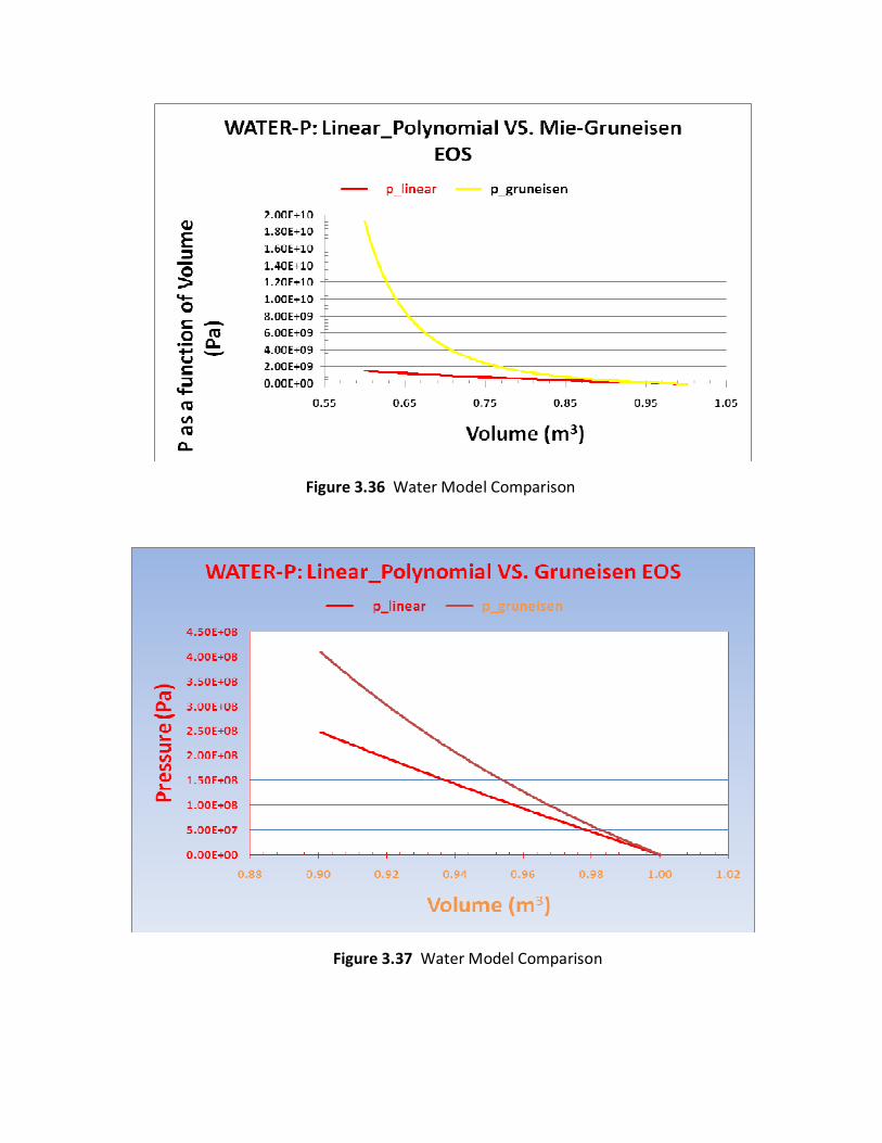
Figure 3.36 Water Model Comparison

Figure 3.37 Water Model Comparison

3.9 Fluids

When modeling materials with little or no shear stiffness, as is the case for fluids, the

default hourglass type (IHQ=1) should be used and the hourglass coefficient should be

greatly reduced (QM=1.0e-6).

3.9.1 Air

In LS-DYNA models in which the physical effects of air are important, *MAT_NULL and

*EOS_LINEAR_POLYNOMIAL are commonly used to represent the air. Typical input

constants for air at sea level (initial pressure = 1 bar) associated with these commands

follow.

*MAT_NULL:

Mass density, RO = 1.0e-9 kg/mm^3

1.0e-3 g/cm^3

1.0 kg/m^3

1.0e-12 tonnes/mm^3

0.94e-7 lbf-s^2/in^4

All other parameters in *MAT_NULL should be set to zero or left blank.

*EOS_LINEAR_POLYNOMIAL:

Unitless parameters C4 and C5 are set to 0.4.

C0 = C1 = C2 = C3 = C6 = 0.

V0 = 1.0

E0 (in units of stress) = initial pressure/C4 = initial pressure/0.4. Thus, for an initial

pressure of 1 bar,

E0 = 2.5e-4 GPa

2.5e-6 Mbar

2.5e+5 Pa

2.5e-1 MPa

36.8 psi

Miscellaneous properties of air (not required in LS-DYNA descriptions given above):

Specific heat, Cp is approximately 1000 J/kg-K

Specific heat, Cv is approximately 717 J/kg-K

Sound speed c = 340 m/s

Bulk modulus K = rho * c^2 = 115,600 Pa

In many ALE applications involving interaction of high density materials, the effects of

air are negligible. In such cases, air can be suitably modeled as void using the simple

material model *MAT_VACUUM instead of using *MAT_NULL and

*EOS_LINEAR_POLYNOMIAL. No input constants are required for *MAT_VACUUM

other than the material ID number.

3.9.2 Water

In LS-DYNA models, *MAT_NULL and *EOS_GRUNEISEN are commonly used to

represent water and other liquids. Some commonly used input constants for water at

20 deg C follow.

*MAT_NULL:

Mass density, RO = 1.e-6 kg/mm^3

1.0 g/cm^3

1000. kg/m^3

1.e-9 tonnes/mm^3

9.37e-5 lbf-s^2/in^4

Dynamic viscosity, MU = 1.0e-3 N-s/m^2 (often taken as 0.0)

Pressure cutoff, PC = -100 Pa (often taken as zero)

All other parameters in *MAT_NULL should be set to zero or left blank.

*EOS_GRUNEISEN:

Nominal sound speed C = 1500 mm/ms

0.15 cm/microsec

1500 m/s

1500e3 mm/s

59055 in/s

E0 = 0

V0 = 1.0 (unitless)

For low pressure applications such as sloshing or fluid flow, the equation-of-state need

only include the above terms. For high pressure situations such as an underwater

explosion, other equation-of-state parameters such as S1, S2, and S3 derived from the

Hugoniot, are usually included in the equation-of-state so as to more accurately

transmit high pressures. Although the pedigree of the following values is not known,

these values are sometimes used for underwater explosion:

S1 = 1.75 (unitless)

S2 = 0 (unitless)

S3 = 0

GAMA0 = 0.28 (unitless)

A = 0 (unitless)

4.0 ALE Modeling Guidelines

In modeling fluid or fluid-like behavior, a Lagrangian approach, wherein the deformation of the

finite element mesh exactly follows the deformation of the material, is often not suitable owing

to the very large deformation of the material. Mesh distortion can, however, become severe,

leading to a progressively smaller explicit time step and eventual instability.

In contrast, an Eulerian or ALE (Arbitrary Lagrangian Eulerian) solution method, wherein the

materials flow (or advect) through the Eulerian/ALE mesh which is either fixed in space

(Eulerian) or moving according to some user-issued directives (ALE), is much better suited to

modeling of fluid or fluid-like behavior.

In LS-DYNA, Lagrangian and Eulerian/ALE solution methods can be combined in the same model

and the fluid-structure interaction (FSI) may be handled by a coupling algorithm. Thus, parts

that deform a moderate amount, such as structural components of metals, composites, or

polymers, can be modeled with Lagrangian elements whereas fluids, such as air and water, and

fluid-like parts, such as birds or ice impacting at high velocity, can be modeled with

Eulerian/ALE elements. Bear in mind that at very high pressure, temperature, and/or strain

rate, even structural materials (metal, concrete, soil, etc.) may behave in a fluid-like manner

and, thus, may be more suitably modeled with Eulerian/ALE elements in such cases.

This section gives an introduction to and general guidelines for modeling with Eulerian/ALE

elements. Modeling of airbags is a special and complex subtopic that is not addressed in this

guidelines document.

4.1 Introduction: Lagrangian vs. Eulerian vs. ALE Formulations

Figure 4.1 shows a 3-frame sequence of a water projectile striking a metal plate. Each row in

this figure represents a different modeling approach and helps to illustrate the fundamental

differences in Lagrangian (1st row), Eulerian (2nd row), and ALE formulations (3rd row). The solid

blue portion represents the water projectile. The red outline is for reference only and marks

the initial, undeformed location of the parts. The LS-DYNA input deck for the model that

produced this figure is: 3in1_impacting_plate_improved.k.

4.1.1 Lagrangian

In an all-Lagrangian approach (3-frame sequence shown in the top row of Figure 4.1), the nodes

move directly along with the material and, thus, elements and materials translate, rotate, and

deform together. Material does not cross element boundaries and, thus, the mass of material

within each Lagrangian element never changes.

4.1.2 Eulerian

In the sequence shown in the middle row of Figure 4.1, the metal target plate is Lagrangian,

however, the mesh of the water and surrounding void is Eulerian and, thus, their mesh remains

fixed in space. The water (shown in solid blue) can move and deform within the fixed mesh. As

the simulation progresses, the materials (water and void) cross element boundaries, i.e., with

each time step some small amount of each material may flow or advect out of one cell (or

element) and into an adjacent cell. At any given point in time, each Eulerian element may

contain a mixture of water and void, hence the term “multi-material” is used in describing the

element formulation. The process by which history variables, e.g., stresses, are calculated

within a mixed element is beyond the scope of this modeling document.

4.1.3 ALE

The third approach, shown in the bottom row of Figure 4.1, employs an ALE formulation in

modeling the water projectile and surrounding void. Again, the metal target is Lagrangian.

Unlike the Eulerian case in which the water and void mesh remain fixed, the ALE mesh is

directed to move in some prescribed manner as the solution progresses. Thus, Eulerian is a

special case of ALE wherein the prescribed reference mesh velocity is zero. Subsequently, we

may refer to this general Eulerian/ALE class of methods as simply “ALE”. Unlike the wholly

Lagrangian case in which the mesh and material move exactly together, the ALE mesh and the

material do not move exactly together. Thus, material advection across element boundaries is

still required, but the amount of material advected each time step is generally less as compared

to the Eulerian approach since the mesh is also moving. Generally the less material that is

advected per time step, the more accurate the simulation. An additional advantage of ALE is

that because the mesh can be directed to approximately follow along with the fluid material(s),

generally fewer elements are needed as compared to the Eulerian approach. In other words,

the entire spatial domain covered over the course of the simulation need not be meshed at the

outset.

Figure 4.1 Water projectile striking a fixed plate using Lagrangian, Eulerian, and ALE

approaches.

4.1.4 Mesh Smoothing

There is a subclass of ALE modeling referred to as mesh smoothing in which the mesh conforms

to the exterior boundary of the ALE material and the elements are reshaped using any of

several smoothing algorithms. After the elements are smoothed, material advection occurs.

Although this smoothing approach is available in LS-DYNA, it is less general and less robust than

the case in which the ALE mesh need not conform to the material boundaries. Thus, the ALE

smoothing approach in LS-DYNA is not discussed any further in these modeling guidelines.

Instead, when ALE is discussed, focus will be on the general ALE approach.

4.1.5 Fluid-Structure Interaction (FSI)

When Euler or ALE parts are required to interact with Lagrangian parts, some form of coupling

(or fluid-structure interaction, FSI) feature must be defined. (The exception is if nodes are

shared between the ALE mesh and the Lagrangian mesh at their juncture – a practice which is

generally not recommended.) ALE-to-Lagrange coupling can be constraint-based, but it is more

commonly penalty-based. The coupling commands in LS-DYNA are discussed in detail later in

this section.

4.1.6 Limitations

There are some limitations to the ALE approach to consider.

The ALE solver in LS-DYNA is predominantly applicable to laminar flow. Also, the ALE solver is

not a full Navier-Stokes solver and, thus, does not account for fluid boundary layer effects such

as drag. Effects of fluid viscosity derive solely via the material model, e.g., via MU in

*MAT_NULL. The ALE solver (ALE compressible flow solver) has been developed with the intent

of simulating short duration problems with high pressure and velocity gradients. The solver is

not well suited to problems driven by low pressure gradients such as in acoustic problems, nor

is it suited to long duration problems (on the order of seconds or longer). The limitation in

time duration is a result of the explicit time integration wherein the time step is limited based

on element size and material speed of sound. In the case of ALE, time step may be further

limited by the penalty stiffness of the ALE-Lagrange coupling.

ALE is relatively expensive as compared to Lagrangian owing to the additional advection,

interface reconstruction, and coupling computations.

Advection associated with the ALE solver is inherently dissipative to some extent, e.g., pressure

amplitude emanating from detonation of explosive tends to be underpredicted, especially

when first order accurate advection is employed (METH = 1 in *CONTROL_ALE). Nonphysical

energy dissipation is generally reduced when second order accurate advection is employed

(METH = 2), but there is some additional computational cost. Refining the mesh also helps to

reduce energy loss, but again there is additional computational cost.

Results from the ALE solver may exhibit some slight to moderate mesh biasing effects. For

example, a pressure wave originating from a point source in a fluid may become less and less

spherical as the distance from the point source increases. This mesh biasing effect is reduced

or eliminated when the mesh lines are parallel and perpendicular to the direction of wave

propagation.

4.2 ALE Element Formulation

When two or more fluids or fluid-like materials (empty space counts as one material) are to be

modeled using the ALE approach in LS-DYNA, the recommended element formulation for those

materials is the multi-material ALE formulation (ELFORM = 11 in *SECTION_SOLID). Although

there are other ALE element formulations (ELFORM 5, 6, and 12), those are of interest perhaps

only in an academic sense and will not be discussed here.

To review, as the ALE materials flow through the ALE mesh, the material boundaries or

interfaces in general do not coincide with the mesh lines. These material interfaces are

internally reconstructed each time step based on the volume fractions of the materials within

the elements. Each material which the user wants to track individually must be assigned a

unique ALE multi-material group (AMMG) ID via the command *ALE_MULTI-MATERIAL_GROUP.

Parts sharing the same material properties may be included in the same AMMG ID or, at the

user’s discretion, can be distributed into separate AMMG IDs to allow for independent tracking

of each group. Materials which do not share the same material properties cannot be part of

the same AMMG.

Generally, some portion of the ALE mesh is initially devoid of material or else is initially filled

with a gas at STP condition (standard temperature and pressure). This void or pseudo-void

provides space into which other, higher density materials may be transported as the simulation

progresses. In our earlier example, water moved with time into elements initially devoid of

material. Space initially devoid of material (and thus having zero mass, zero pressure, etc.) is

modeled with *MAT_VACUUM. If the space is occupied by air or some other ideal gas with

nonzero density, with or without nonzero pressure, a material model and an equation-of-state

appropriate for such a gas, e.g., *MAT_NULL and *EOS_IDEAL_GAS, should be assigned to that

space.

Motion of the ALE mesh is controlled by the family of command(s)

*ALE_REFERENCE_SYSTEM_OPTION. Without such a command, the ALE mesh will remain

stationary, thus becoming the special case of Eulerian. Using these commands, one can

prescribe the motion of the ALE mesh in a very specific and/or predetermined manner, or the

mesh motion can be made to approximately follow the mass-weighted average velocity of the

ALE materials. This latter option is perhaps the most common and useful choice, and it is

invoked by setting PRTYPE=4 in *ALE_REFERENCE_SYSTEM_GROUP.

Since the ALE method allows for materials to flow between elements and the user has direct

control over the ALE mesh motion, ALE element distortion is generally of no concern. It follows

that hourglass deformation is less of an issue in the case of ALE than in the case of Lagrangian,

and the need for hourglass forces to restrict hourglass deformation is much reduced or

eliminated. For materials modeled as ALE, hourglass formulation 1 and a much reduced

hourglass coefficient, e.g., 1.0E-6 or less, are recommended to prevent application of

inappropriate hourglass forces. This recommendation is especially true in the case of modeling

gases and liquids. Starting in version 971 R3.1, the default hourglass coefficient for all parts

with ELFORM=11 is set to 1.E-06. The default hourglass control can always be overridden by

the user using *HOURGLASS and HGID in *PART. Such an override may be appropriate in the

case of solid (non-fluid) ALE materials.

4.3 Meshing

Hexahedral elements with reasonable aspect ratios should be used for the initial ALE mesh.

Degenerate element shapes, such as tetrahedrons and pentahedrons, should be avoided as

they may lead to reduced accuracy at best and perhaps numerical instability during the

advection. Bear in mind that use of * ALE_REFERENCE_SYSTEM may affect the element shapes

as the solution progresses. If element shapes become unreasonable, controls in the

*ALE_REFERENCE_SYSTEM_OPTION command(s) may need to be adjusted to maintain

reasonable element shapes.

An initial ALE mesh may be constructed using one of the following two approaches:

• The initial mesh of the ALE domain may be constructed to conform to the materials, i.e.,

there are no mixed (or partially filled) cells in the initial configuration. Mesh lines follow

the outer contour of each AMMG.

• A regular, orthogonal mesh of the ALE domain may constructed with no restriction that

mesh lines follow the outer contour of each AMMG. In this case, there will likely be

elements containing more than one AMMG. For these mixed elements, the initial

volume fractions of AMMGs must be prescribed via

*INITIAL_VOLUME_FRACTION(_GEOMETRY). This command has a "geometry" option

that automates the assignment of initial volume fractions to ALE elements. At the

conclusion of the automatic assignment of initial volume fractions, LS-DYNA writes a file

containing the * INITIAL_VOLUME_FRACTION data for each ALE element before

continuing with the simulation. This file can be utilized in subsequent runs in lieu of the

* INITIAL_VOLUME_FRACTION_GEOMETRYcommand, thereby speeding up initialization.

What constitutes an appropriate degree of refinement for the ALE mesh is at least partially

dictated by the geometric characteristics of the Lagrangian parts. Though not a requirement, a

reasonable goal is to have the ALE elements be nearly the same size as the Lagrangian elements

where coupling is to take place.

If ALE material is to flow through any passages in the Lagrangian mesh, use at least 5 to 10

elements across the passage width in order to adequately resolve the flow. Consider as a

guideline using a number of elements across the passage equal to the points necessary to

resolve a parabolic shape such that the area of the parabola is preserved to the user’s required

accuracy.

As stated under the limitations section above, results may exhibit some mesh bias. If these

effects appears to be significant, reconstruction of the initial mesh and controls on mesh

movement (*ALE_REFERENCE_SYSTEM_OPTION) may be warranted.

4.4 Coupling Lagrangian Surfaces to ALE Materials

Most often, in Fluid-Structure Interaction (FSI) problems modeled with LS-DYNA, the fluids (and

sometimes other materials that behave in a fluid-like manner) are modeled with ALE

hexahedrons and the structure is modeled with Lagrangian shells or solids. In such a model, the

Lagrangian mesh usually does not share nodes with the ALE mesh. Rather, the two meshes

interact via a coupling algorithm defined with the command

*CONSTRAINED_LAGRANGE_IN_SOLID. This coupling serves to generate forces that resist

penetration of the ALE material through the Lagrangian parts. Coupling is a key and sometimes

complex aspect of ALE modeling. Some recommendations for using

*CONSTRAINED_LAGRANGE_IN_SOLID for coupling are provided below.

Let us consider some of the more critical parameters of the

*CONSTRAINED_LAGRANGE_IN_SOLID card:

$-------------------------------------------------------------------------------

*CONSTRAINED_LAGRANGE_IN_SOLID

$ slave master sstyp mstyp nquad ctype direc mcoup

1 200 1 0 2 4 2 -1

$ start end pfac fric frcmin norm normtyp DAMPFRAC

0.0 0.0 0.100000 0.0 0.300000

$ cq hmin hmax ileak pleak lcidpor

0.0 0.0 0.0 0 0.10000

$4A IBOXID IPENCHK INTFORC IALESOFT LAGMUL PFACMM THKF

0 0 1 0 0 0 0.0

$-------------------------------------------------------------------------------

The slave side parameters SLAVE and SSTYP identify the Lagrangian part(s) or segment sets to

be considered in the coupling. The master side parameters MASTER and MSTYP identify, by

part or part set ID, the ALE mesh that will interact with the slave side. Again, the master side

identifies mesh, but not material. Together, SLAVE, SSTYP, MASTER, MSTYP define the

overlapping computation domains (Lagrangian and ALE) that the code will search for interaction.

This does not yet specify which ALE material(s) flowing through the ALE domain are to be

coupled to the Lagrangian structure.

A separate parameter MCOUP identifies the specific ALE materials, or more precisely, the

AMMGs that will interact with the slave side.

To summarize coupling thus far, for coupling forces to be developed on a Lagrangian surface,

(1) that surface must reside on the slave side of a * CONSTRAINED_LAGRANGE_IN_SOLID, (2)

that surface must be spatially overlapping a portion of the ALE mesh identified by the master

side, and (3) that surface must be penetrating at least one of the AMMGs identified by the

parameter MCOUP. See below for more discussion of MCOUP.

The parameter NQUAD determines the number of coupling points distributed over each

Lagrangian slave segment. If NQUAD=2 (default), then there are 2x2 = 4 coupling points on

each Lagrangian slave segment. The coupling algorithm looks for penetration of any ALE

material meeting the conditions of MASTER, MSTYP, and MCOUP across each of the coupling

points. If penetration at a coupling point is found, coupling forces are applied to counteract

penetration. The larger the value of NQUAD, the more expensive the coupling and the more

likely the coupling forces will be excessive. If the Lagrangian slave segments are approximately

the same size as or smaller than the Eulerian/ALE element faces, NQUAD=2 will generally

suffice. If the Lagrangian slave segments are coarser/larger than the ALE element faces,

NQUAD may need to be raised to 3 or higher to provide proper coupling.

The parameter CTYPE identifies the coupling algorithm employed. In most applications, penalty-

based coupling is more robust and is therefore preferred over constraint-based coupling. Thus,

CTYPE should generally be set to 4, or in the case where the Lagrangian slave side is comprised

of solids which may be eroded due to material failure criteria, CTYPE should be set to 5. There

are other CTYPEs that allow for physical porosity of the Lagrangian surfaces, e.g., as in the case

of an airbag or parachute, but a discussion of modeling porosity effects is outside the scope of

this document. For the special case of coupling Lagrangian beam elements within a Lagrangian

solid mesh, e.g., as used in coupling rebar to concrete, the constraint-based coupling algorithm

should be used (CTYPE=2).

The parameter DIREC should generally be set to 2 as this most often best represents the

physical nature of the interaction. Furthermore, it is also the most reliable and robust option.

With DIREC=2, normal direction coupling occurs only in compression. Tangential coupling,

associated with friction between materials, is controlled separately via the parameter FRIC.

The parameter MCOUP defines the AMMG(s) to which the Lagrangian slave side is coupled. In

cases where one AMMG dominates the forces imparted to the Lagrangian structure and the

forces from any other AMMGs can be neglected, MCOUP should be set to 1. This might be the

case where the density of one AMMG is far greater than the density of the other AMMGs. In

cases where the effects of two or more AMMGs need to be considered in the coupling, MCOUP

can be set to a negative number. In this case, |MCOUP| identifies a set of one or more AMMGs

to be considered in the coupling. That set is defined using the command *SET_MULTI-

MATERIAL_GROUP_LIST.

When the slave side of the coupling is comprised of Lagrangian shells or of a segment set

comprised of Lagrangian element faces, an additional requirement of successful coupling is that

the slave shell/segment normals must point toward the AMMGs to which coupling is desired. If

the slave side normals happen to point away from the AMMGs, these normals can be

automatically reversed and the situation remedied by setting the parameter NORM=1. Note

that setting NORM to 1 reverses all the normals of the Lagrangian slave segments. Thus, it is

imperative that the slave segment normals are at least consistently oriented either pointing

toward (NORM=0) or away from (NORM=1) the ALE material.

Leakage is an undesireable condition whereby coupling does not prevent unreasonable

penetration of ALE material through Lagrangian surfaces. Problems of leakage can be

identified visually when post-processing which will be described in a later section. A small

amount of leakage is to be expected and can be tolerated for penalty-based coupling,

analogous to the case of small penetrations that are observed for penalty-based contact. The

following modifications to the coupling input are presented as possible remedies to excessive

leakage:

• Increase the value of NQUAD if it is suspected that there are too few coupling points on

the Lagrangian segments. Be judicious here because increasing NQUAD drives up the

cpu time.

• When coupling to a shell surface, assign one AMMG ID to the ALE material on one side

of the shell surface and a different AMMG ID to the ALE material on the opposite side.

Of course, this practice is a requirement if there are two physically different materials to

either side. The point is that this guideline applies even when the same physical fluid

exists on both sides of the shell surface.

• Use a separate * CONSTRAINED_LAGRANGE_IN_SOLID command for each AMMG. This

will require the use of a negative MCOUP value and a *SET_MULTI-

MATERAIL_GROUP_LIST mcommand for each * CONSTRAINED_LAGRANGE_IN_SOLID

command.

• An appropriate coupling stiffness is key to good coupling behavior when CTYPE=4 or 5.

In most cases, the default penalty stiffness (PFAC=0.1) works fine and this should be the

starting point. If it becomes clear that the default coupling stiffness is inadequate,

simply increasing PFAC (by 5 or 10 times) might resolve the problem. A more logical

approach is to set PFAC to a negative integer, which tells LS-DYNA that the coupling

stiffness comes from curve |PFAC| wherein the abscissa is penetration distance and the

ordinate is coupling pressure. *DEFINE_CURVE should be used to define curve |PFAC|.

(For example, assume PFAC=-20. Then curve 20 defines coupling pressure vs.

penetration distance.) A rule-of-thumb in defining the curve is to define two points:

(0,0) and (1/10th the ALE element dimension, maximum pressure observed in the ALE

mesh near the leakage site). Be aware that an increase in coupling stiffness may result

in a smaller time step size. Just as far too small a coupling stiffness has detrimental

effects, so does far too great a coupling stiffness.

• For coupling of ALE gases to Lagrangian parts (low-density-to-high-density materials), it

may help to set the parameters ILEAK=2 and PFACMM=3.

As a final word in modeling coupling between ALE and Lagrangian parts, there is a coupling

method that may serve as a preferred alternative to * CONSTRAINED_LAGRANGE_IN_SOLID in

some cases. *ALE_FSI_PROJECTION uses a constraint-based approach, projecting the nearest

ALE nodes onto the Lagrangian surface. Coupling can be in all directions, in tension and

compression only, or in compression only. Energy is not conserved in this approach, but it has

been shown to be effective in coupling fluid to tank walls in a sloshing tank simulation. An

example in which only gravity is applied to develop hydrostatic pressure in a tank of water is

init_water_coupled_to_tank_fsi_projection.k. Figure 4.2 shows the hydrostatic state at the end

of the simulation.

Figure 4.2 The hydrostatic state in a tank of water.

In the next two examples, the container moves horizontally to introduce sloshing of the water;

init_water_coupled_to_tank_fsi_projection_with_sloshing_2couplings.k uses

*ALE_FSI_PROJECTION to couple the water to the tank; init_water_coupled_to_tank_

with_sloshing.k uses penalty-based * CONSTRAINED_LAGRANGE_IN_SOLID to couple the water

to the tank as shown. Similar results from the two simulations are shown in Figures 4.3 and 4.4

Figure 4.3 Results for init_water_coupled_to_tank_fsi_projection_with_sloshing_2couplings.k.

Figure 4.4 Results for init_water_coupled_to_tank_ with_sloshing.k.

4.5 Modeling Inflow and Outflow Conditions

In addition to setting ELFORM to 11, setting AET to 4 in *SECTION_SOLID invokes a reservoir (or

ambient) type element option in the ALE formulation. The user may dictate pressure to such

elements by prescribing the thermodynamic condition of the element, either as unvarying with

time by simply defining E0 and V0 in the *EOS (equation-of-state) input or as a function of time

via *BOUNDARY_AMBIENT_EOS. Thus, to model a prescribed inflow or prescribed outflow of

material, one or two layers of ALE elements on the exterior of the mesh at the inflow (outflow)

region is assigned a unique PART ID so that AET may be set to 4 for that layer. If the inflow or

outflow conditions include a known flow velocity into or out of the ALE mesh, that velocity is

prescribed by applying *BOUNDARY_PRESCRIBED_MOTION_NODE to the exterior nodes at the

inflow/outflow region.

To model unprescribed (unknown) outflow, AET may be left as 0 (default) in which case outflow

is calculated by LS-DYNA.

Do not attempt to assign values other than 0 or 4 to the parameter AET.

An example input file illustrating prescribed inflow is: purge.ambient.mod.k . Figures 4.5, 4.6,

and 4.7 show snapshots of the simulation. In this example, inflow of water into an empty

container is diverted by a rubber flap modeled with Lagrangian solids. The rigid “container” is

simulated via nodal constraints, i.e., the container is not represented by elements. An egress

hole in the container is included by leaving some of the exterior nodes in the lower right-hand

corner unconstrained in the horizontal direction. By virtue of their ambient inflow designation

(AET=4), the pressure is prescribed in the top layer of elements and that, together with gravity

loading, serves to drive the simulation. Because *BOUNDARY_AMBIENT_EOS is not used in this

example, the prescribed pressure in the ambient elements is a constant value, determined from

the initial condition parameters in the equation-of-state.

Figure 4.5 purge.ambient.mod.k at time=0.


4.6 Pressure Initialization in ALE Materials

In many situations, an initial pressure field in one or more of the ALE materials is known, e.g.,

atmospheric pressure in air or hydrostatic pressure in water. If the pressure field is uniform as

in air at atmospheric pressure, EO and V0 in the *EOS input is sufficient to initialize the pressure.

In such a case, as mentioned earlier, exterior segments must also have an applied pressure to

equilibrate the internal pressure, either via *LOAD_SEGMENT or via PREF in *CONTROL_ALE.

In the more complex case where pressure varies with depth as in the case of water, the

command *INITIAL_HYDROSTATIC_ALE can be used as an aid to greatly reduce the time it takes

to initialize the hydrostatic pressure and reach a steady state condition in the fluid.

An example of a pool-like condition without inflow or outflow conditions is f_damp300_bub.k.

In this example, a gas bubble initially resides below the surface of the water as shown in Figure

4.8.

Figure 4.8 Gas bubble below in the surface in f_damp300_bub.k.

*INITIAL_HYDROSTATIC_ALE, in conjunction with *LOAD_BODY, which applies gravity loading,

and *BOUNDARY_SPC, which applies the normal direction constraints to the pool walls and

pool bottom, serves to quickly initialize the hydrostatic state of the fluids. In addition, this

example employs mass damping (*DAMPING_PART_MASS) to remove the oscillations in

pressure time histories that are otherwise seen when no damping is employed. The damping is

specified as a function of time and is set to zero after achieving a steady state condition (t =

0.08 in this example) so as not to inhibit physical motion thereafter. If the termination time in

the example is extended from 0.2 to 2.0, such motion is clearly evident in the form of the gas

bubble rising and changing shape. Note that when mass damping is used, the value should be

derived from the period of oscillation T, recognizing that critical damping is equal to 4π /T.

Figures 4.9 and 4.10 show the early time results of the example. For more details on this

example and of the *INITIAL_HYDROSTATIC_ALE command syntax, see pp. 14-25 of the tutorial

“Simulating Hydrostatic Pressure”.

Figure 4.9 Pressure contours of gas bubble in water at t=.2 sec.

Figure 4.10 Time history plots of pressure.

An example where, instead of nodal constraints be applied to invoke a pool-like condition

without inflow or outflow, a layer of reservoir/ambient elements (AET=4) are defined along the

sides and bottom of the ALE mesh to permit inflow and outflow of fluid is

g_damp300_bub_AAH_.rising.k. Such a condition would be appropriate if modeling a body of

water in which the water level is changing with time in a known manner in the far field, i.e., at a

location where pressure is virtually unaffected by dynamic behavior, including fluid/structure

interaction, taking place in the near field. In the example, a gas bubble initially resides below

the surface of the water but this time is coupled to a fixed cylindrical container so that the

bubble cannot rise. As before, gravity is applied via *LOAD_BODY and temporary mass damping

is applied via *DAMPING_PART_MASS. The initial condition is seen in Figure 4.11.

Figure 4.11 Initial condition for a gas bubble below the surface of water.

*INITIAL_HYDROSTATIC_ALE is again used to initialize the hydrostatic pressure in the

nonambient fluid field and an additional command, *ALE_AMBIENT_HYDROSTATIC, is used to

prescribe the fluid pressure in the ambient elements along the sides and bottom of the fluid

field. The command syntax of * ALE_AMBIENT_HYDROSTATIC is identical to that of

*INITIAL_HYDROSTATIC_ALE and is shown on p. 30 of the tutorial “Simulating Hydrostatic

Pressure”. The pressure in the ambient elements is automatically computed based on the

location of the top surface of each fluid as tracked by nodes selected by the user. In this

example, a massless node ID 100000 is given a prescribed velocity in the vertical (y) direction to

control the top surface of the water in the ambient elements along the sides of the mesh. The

resulting y-displacement of node 100000 is shown in the Figure 4.12.

Figure 4.12 Y-Displacement of surface node 100000.

The effect of * ALE_AMBIENT_HYDROSTATI is that, as the water height changes, the pressure in

each ambient element changes accordingly. The change in pressure of the ambient elements

drive pressure gradients through fluid field causing the water level to change in the main body

of the fluid mesh. The change in water level (green material) can be seen Figures 4.13 and 4.14.

Figure 4.13 Water level at t=1.34 sec.

Figure 4.14 Water level at t=6 sec.

Figure 4.15 shows pressure fringes and Figure 4.16 shows pressure time histories. Note the

difference in character between the pressure time histories of the ambient elements (smooth,

as prescribed by * ALE_AMBIENT_HYDROSTATIC) and the pressure time histories of the

elements in the nonambient fluid field (not quite as smooth).

Figure 4.15 Pressure contours.

Figure 4.16 Pressure time history of selected elements.

4.7 Post-Processing

Because ALE materials do not follow the mesh and can migrate from part to part, viewing the

location of ALE materials when post-processing is a little different than viewing Lagrangian

materials. Lagrangian material is tracked by part ID. ALE material is tracked by AMMG ID.

When post-processing the d3plot database with LS-PrePost, one can view any of the AMMGs by

selecting Selpar > Fluid. Each AMMG is then added to the Part Selection list so that it may be

selected and viewed just as one might select and view a part.

Alternately, the location of each AMMG can be seen by fringing volume fraction of the

respective AMMG. A volume fraction of 0.0 in a region indicates the complete absence of the

AMMG in that region. A volume fraction of 1.0 in a region indicates that the region is

completely filled with that AMMG. A number between 0.0 and 1.0 means the region is partially

filled with that AMMG and, thus, partially filled with one or more other AMMGs. For example,

to see where material associated with AMMG #2 resides, one could click Fcomp > Misc >

volume fraction mat#2. The space shown in red (corresponding to fringe values between 0.9

and 1.0) is the space exclusively or predominantly occupied by AMMG #2.

Fcomp > Misc > dominant fluid material identifies the various AMMGs by assigning a value of

1.0 to those cells comprised predominantly of AMMG 1, 2.0 to those cells comprised

predominantly of AMMG 2, and so on.

History > Element > species mass mat#n plots a time history of the mass of AMMG #n in the

selected element. The total mass of the element is the sum of all the species masses.

In the case of an ALE element, the seven standard history variables written to the d3plot

database and labeled as x-stress, y-stress, z-stress, xy-stress, yz-stress, zx-stress, and plastic

strain in LS-PrePost are the volume-fraction-weighted values of those respective components.

In other words, for an element which has a mix of AMMG 1 and AMMG 2 and which contains

no other AMMG, the x-stress in that element will be (element x-stress in AMMG 1)*(volume

fraction of AMMG 1) + (element x-stress in AMMG 2)*(volume fraction of AMMG 2).

As with any element, pressure, effective stress (von Mises), etc. are not contained in d3plot, but

rather are computed by LS-PrePost using the x-stress, y-stress, … , zx-stress values from d3plot.

Thus, for an ALE element, pressure, effective stress, etc. are calculated based on the volume-

fraction-weighted x-stress, y-stress, etc.

In addition to the seven standard history variables, each material model has a particular

number of so-called extra history variables which can optionally be written to d3plot. When

post-processing with LS-PrePost, any saved extra history variables are listed under Fcomp >

Misc and under History > Element as “history var#1”, “history var#2”, and so on. Whether

dealing with Lagrangian or ALE parts, the number and meaning of the extra history variables for

each material model is specific to that material model. To write these extra history variables,

NEIPH in *DATABASE_EXTENT_BINARY must be set to the number of extra history variables

desired. The bookkeeping scheme used in writing extra history variables gets complex with

multi-material ALE parts included in the model and it is best explained by way of an example.

When there are ALE parts in the model, useful information about the stored extra history

variables can be ascertained from the messag file, e.g., the messag file might say…

*** Note history variables in lsprepost --> Fcomp -->misc

history variable 1 to 4 belongs to AMMG 1




These statements warrant some explanation. First, know that AMMG 1 is always unique in the

sense that the seven standard history variables are not written for AMMG 1. The statement in

d3hsp "history variable 1 to 4 belongs to AMMG 1" means that the first four extra

history variables in the database are the four extra history variables associated with the

material model of AMMG 1. Again, the number and meaning of extra history variables is

specific to that particular material model. (Bear in mind that most of the extra history variables

for any given material model are of little or no interest to the engineer. Only occasionally will

the engineer be interested in extra history variables, e.g., those representing damage and

temperature in *MAT_015.) The statement "history variable 5 to 14 belongs to AMMG

2" indicates that a total of ten history variables (labeled as history var#5 to history var#14 in LS-

PrePost) are written for AMMG 2. There are seven standard history variables written for each

AMMG (excepting AMMG 1 as noted above), thus the first seven history variables written for

AMMG 2 (history var#5 to history var#11) are these seven standard history variables (x-stress,

y-stress ..., plastic strain) for AMMG 2 and the subsequent three (history var#12 to history

var#14) are extra history variables associated with the material model of AMMG 2. In like

fashion, history var#15 to history var#21 are x-stress, y-stress, … , plastic strain for AMMG 3 and

history var#22 to history var#26 are extra history variables associated with the material model

of AMMG 3. Finally, history var#27 to history var#33 are x-stress, y-stress, … , plastic strain for

AMMG 4 and history var#34 to history var#39 are extra history variables associated with the

material model of AMMG 4.

Please note that to actually write 39 extra history variables to the d3plot database (4 for AMMG

1 + 10 for AMMG 2 + 10 for AMMG 3 + 13 for AMMG 4 = 39 total), NEIPH must be set to 39 in

*DATABASE_EXTENT_BINARY.

When using Fcomp to view history variables in ALE parts, it's sometimes clearer to view

isosurfaces rather than fringes. To invoke isosurface viewing, click on the Frin button and

choose Isos.

Aside from the d3plot database, there are other output files which can be useful in post-

processing ALE simulations:

• dbfsi is an ASCII output file created when *DATABASE_FSI is included in the input deck.

The dbfsi file reports time histories of coupling forces applied to the Lagrangian surface

identified on Card 2 of * DATABASE_FSI. These coupling forces arise from the penalty-

based coupling defined in *CONSTRAINED_LAGRANGE_IN_SOLID. The dbfsi file also

reports coupling pressure, defined as the net, normal coupling force divided by the

Lagrangian segment area, and mass flux (mflux), defined as the accumulated ALE

material mass moving past a set of segments. Mflux can be used to track leakage if the

segments are Lagrangian or advection if the segments are ALE. Mflux is also useful for

tracking the mass of material exiting a vent hole.

• dbsensor is an ASCII output file containing time histories of pressure at sensors located

in the ALE mesh. The command * DATABASE_FSI _SENSOR defines the sensors and

specifies the output time interval. Each pressure sensor follows along with a Lagrangian

segment (this segment must be included in the slave side of a

*CONSTRAINED_LAGRANGE_IN_SOLID coupling definition). Optionally, the sensor may

be offset a specified distance from the Lagrangian segment in the normal direction.

• trhist is an ASCII output file containing stress and pressure time histories and is created

when database_tracer is included in the input deck. A tracer is very similar to a sensor,

but a tracer does not follow a Lagrangian segment. A tracer can be fixed in space or else

made to follow the ALE material.

• fsifor is a binary database created when the print flag is set in field 3, Card 4 of

*CONSTRAINED_LAGRANGE_IN_SOLID and a database name is given on the LS-DYNA

execution line using “h=dbasename”. The binary database can be read into LS-PrePost

to enable fringe plots of coupling pressure on the Lagrangian surface, as well as time

history plots of coupling pressure and forces on segments.

4.8 Troubleshooting

Experience has shown that simulations that include ALE elements commonly need to have the

time step scale factor (TSSFAC in *CONTROL_TIMESTEP) reduced from the default of 0.9 to

somewhere around 0.6 in order to maintain a stable solution.

Excessive leakage of ALE material across Lagrangian surface:

See discussion of coupling in section 4.4.

Negative sliding energy attributable to coupling:

Energy associated with * CONSTRAINED_LAGRANGE_IN_SOLID coupling is calculated and

included in “sliding interface energy” reported to glstat. This coupling energy is not, however,

reported to sleout. Thus, the difference between sliding interface energy in glstat and total

sliding energy in sleout is the coupling energy. If the coupling energy is negative and exhibits a

significant influence on the overall energy balance, i.e., the energy ratio drops due to the

negative coupling energy, possible improvements may be seen by (1) refining the ALE mesh, (2)

reducing the time step scale factor, and/or (3) reducing FRCMIN in *

CONSTRAINED_LAGRANGE_IN_SOLID, e.g., from 0.5 to 0.25.

Negative volume in advection:

This error can occur when the amount of material moving in/out of an ALE element during the

advection is excessive. The possibility of this happening is diminished when NADV is set to 1 in

*CONTROL_ALE (recommended). If the error still occurs when NADV=1, consider the following

possible remedies:

• Reduce the time step scale factor TSSFAC.

• Refine the mesh (which in itself may reduce the time step) and, if any ALE elements are

poorly shaped, improve the mesh quality. Often, a regular ALE mesh with cubical or

nearly cubical elements is a good starting point.

• Check material input, especially the material density.

• Use appropriate boundary conditions on the exterior of the ALE mesh. Such boundary

conditions would usually consist of either (a) nodal constraints to prevent material from

exiting the mesh, or (b) pressure applied on the exterior segments to resist egress of

material. The former can be applied manually using *BOUNDARY_SPC or automatically

using EBC in *CONTROL_ALE. The latter (pressure boundary condition) can be applied

manually using *LOAD_SEGMENT or automatically using PREF in *CONTROL_ALE.

• Excessive/inappropriate coupling forces could trigger high material velocity. Review the

coupling input, making sure that the Lagrangian segment normal directions are

appropriate and that the coupling stiffness is not excessive.

Time step drops dramatically:

This problem is often the result of too little mass in an element, perhaps due to excessive

material velocity. If the element controlling the time step is near the exterior of the ALE mesh,

see the bullet above on appropriate boundary conditions.

5.0 Aerospace Applications

This section of the document reviews some specific aerospace applications and provides

guidelines and methodologies for those applications.

In general, aerospace applications generally involve higher strain rates than other

impact events. Thus, there is a highly likelihood that the default time step size will be

too large to ensure stability. Often, the time step scale factor TSSFAC in

*CONTROL_TIMESTEP will need to be reduced, e.g., to a value of 0.6 or less, when

modeling aerospace events. The greater the relative impact velocity, the more that

TSSFAC will need to be reduced.

5.1 Stress Initialization for Spinning Bodies

A blade that rotates at a constant speed is subject to a constant centrifugal body force

with the magnitude

F = m*(omega**2)*Rcg

where F is the centrifugal force, m is the blade mass, omega is the rotational velocity,

and Rcg is the radius to the center of gravity. This is a static load and the resulting stress

in the blade is a constant and is referred to as the blade pre-stress. The term objective

stress is used to describe the behavior that this stress is invariant with respect to rigid

body rotation.

The following sections define the procedures for applying the centrifugal force in an

implicit pre-stress static solution, rotating the blade in an explicit transient solution, and

unloading the blade in an implicit static solution. Following these procedures will result

in a correct and stable solution for a rotating blade for use in subsequent bird-strike or

blade-off analyses. A validation of the constant root cross-section force and the

element stresses is also demonstrated.

It should be noted that alternate approaches are available in LS-DYNA to incorporate

pre-stress for a rotating blade including dynamic relaxation; reading in displacements

from a another implicit solver (e.g., ANSYS, NASTRAN); ramping up the blade rpm in a

transient solution and applying damping to obtain a stable solution; but the approach

using the LS-DYNA implicit and explicit solvers discussed below is the most robust.

Whatever the approach selected, it is recommended that a check for a stable solution

be completed.

5.1.1 Implicit Pre-stress Static Solution

For the implicit pre-stress static solution the blade is fixed at the root to remove all rigid

body rotation and the blade centrifugal load is applied by specifying blade rpm. The

output from this implicit analysis is the dynain file which contains the blade deformed

geometry (both nodes and elements) and stress state. This dynain file is then used as

input for the explicit transient analysis.

All element formulations for shell and brick elements can now be used with the implicit

solver. The same element type should, however, be used in the implicit and explicit

analyses to avoid numerical instabilities at the start of the explicit transient analysis.

The *LOAD_BODY keyword input is used to define the centrifugal body force load. This

input has options RX, RY, and RZ that allow definition of the load with respect to any of

the coordinate axes. This input references a load curve that is defined using the

*DEFINE_CURVE keyword input that contains the blade speed in radians/time versus

time. This curve is defined from time 0 to 1.0 with a rotational velocity from 0 to the

desired pre-stress rotational velocity. It should also be noted that this body force load is

applied to all nodes in the complete problem unless a part subset is defined using the

*LOAD_BODY_PARTS keyword input.

The termination time of the analysis should be set to 1.0 using the

*CONTROL_TERMINATION keyword input.

To select the implicit solver use the *CONTROL_IMPLICIT_GENERAL keyword input and

set the variable IMFLAG=1.

Use the *INTERFACE_SPRINGBACK_LSDYNA keyword input to output the dynaini file.

As previously mentioned, boundary conditions to eliminate rigid body motion are

required. A set containing the root nodes of the blade can be defined using the

*SET_NODE keyword input. The root translational and rotational degrees of freedom

are then constrained in the appropriate direction using the

*BOUNDARY_PRESCRIBED_MOTION_SET input. This input references a curve defined

using the *DEFINE_CURVE input that has the prescribed displacement of 0.0 defined for

all time 0 to 1.0. Alternately, *BOUNDARY_SPC_SET can be used to constrain the

degrees of freedom of the root nodes in the node set. The method of constraining rigid

body modes changes if the root nodes are included as part of a rigid hub. In this case,

*BOUNDARY_PRESCRIBED_MOTION_RIGID is used to constrain the degrees of freedom

of the rigid hub.

To aid in validating the stress initialization solution, a cross-section at the root of the

blade should be defined. The cross-section is defined using the

*DATABASE_CROSS_SECTION_SET input. A set of the root elements and nodes should

be defined using the *SET_ELEMENT and *SET_NODE options and those sets are then

referenced on the cross-section input. The output frequency of the cross-section forces

is defined using the *DATABASE_SECFORC input. An SECFORC file for output post-

processing in then generated.

The double precision version of LS-DYNA should be run when using the implicit solver.

An example keyword file for the implicit prestress is: blade_preload.k

5.1.2 Explicit Transient Rotation

Using the dynain file output from the implicit solution, a new input file is created to

rotate the blade for one revolution to demonstrate a stable solution for cross-section

force output and stress state. This input can also be used for bird-strike and blade-off

analyses.

The termination time on the *CONTROL_TERMINATION input should be defined to

correspond to one revolution.

Use *INITIAL_VELOCITY_GENERATION input to have the code calculate and apply the

nodal velocities for rotation. The PHASE=0 option, which is the default, should be

specified to have the nodal velocities calculated immediately at the start of the

transient. The rotational velocity in radians/time should correspond to and take the

place of the applied body force load applied in the implicit pre-stress analysis.

Following the above procedure, the spinning blade(s) should be in a state of equilibrium

and the resultant velocity of any node should be constant with time assuming there are

no external forces applied to the blades. If, in a production simulation, external forces

are applied, e.g., as from a bird strike, rotational velocity of the blade root nodes can be

enforced as a function of time using *BOUNDARY_PRESCRIBED_MOTION_SET input with

option 9, 10, or 11 selected depending on the axis of revolution. The axis of revolution

should correspond with the applied body force load in the implicit solution. The node

set should be the identical root node set as defined in the implicit solution. This input

references a curve that has the prescribed rotational velocity defined in radians/time

versus time.

The *CONTROL_ACCURACY keyword input needs to be included with the objective

stress update on (OSU=1) and invariant node numbering on with INN=2 for shells, INN=3

for solids, and INN=4 for both shells and solids.

If shell elements are used, the input parameter to update the shell normal as the blade

rotates must also be included for shell formulations 1, 6, and 7. This is achieved by

setting the parameter IRNXX=-2 on the *CONTROL_SHELL keyword input.

The *DATABASE_CROSS_SECTION input should also be included as in the implicit

solution to monitor the root cross-section forces as the blade rotates.

Use the *INTERFACE_SPRINGBACK_LSDYNA keyword input to generate the dynain

output file for completing the unload step.

The single precision version of LS-DYNA can be run when using the explicit solver.

An example keyword file for the explicit rotation is: blade_rotate.k

5.1.3 Stable Solution Check

To check for a stable solution the root cross-section forces and element stresses are

plotted. Figure 5.1 shows the sinusoidal variation in the root cross-sectional force as the

blade rotates about the z-axis. The resultant force is a constant as the blade rotates and

it should check with the hand calculation for blade pull. Figure 5.2 shows that the root

element stresses are constant when plotted in a local coordinate system that is rotating

with the blade. The von Mises stress is invariant with respect to rigid body rotation as is

demonstrated in Figure 5.3. With a stable solution for the rotating blade obtained, the

blade model can now be used in a bird-strike or blade-off analysis.

It should be noted that the dynain file is written at the termination of the analysis

whether it is a simple stable solution check or a more complex bird-strike or blade-off

analysis. This dynain file can then be used in a subsequent implicit static unload analysis

where the centrifugal force is removed.

Figure 5.1 Root Cross Section Forces.

Figure 5.2 Root Element Stress.

Figure 5.3 Root Element Von Mises Stress.

5.1.4 Implicit Static Unload Solution

The rotating blade is unloaded in an implicit static unload analysis that is the opposite of

the load analysis. If the unload step is completed at the end of the stable solution

check, a blade identical to the original blade at the start of the analysis with zero stress

should result. If the unload step is completed at the end of a bird-strike or blade-off

analysis, the final deformed shape of the blade will result for comparison to actual test

results.

The *LOAD_BODY keyword input with the appropriate rotation axis (RX, RY, or RZ) is

used to remove the centrifugal body force load just like it was used to apply the load.

The difference, however, is that the load curve for this analysis will be defined from time

0 to 1.0 with the rotational velocity defined from the rotating speed in radians/time to

0.

The termination time of the analysis should be set to 1.0 using the keyword

*CONTROL_TERMINATION input.

To select the implicit solver use the *CONTROL_IMPLICIT_GENERAL keyword input and

set the variable IMFLAG=1.

As in the load step, boundary conditions to eliminate rigid body motion are required. A

set containing the root nodes of the blade can be defined using the *SET_NODE

keyword input. The root translational and rotational degrees of freedom are then

constrained in the appropriate direction using the

*BOUNDARY_PRESCRIBED_MOTION_SET input. This input references a curve defined

using the *DEFINE_CURVE input that has the prescribed displacement of 0.0 defined for

all time 0 to 1.0.

The double precision version of LS-DYNA should be run when using the implicit solver.

An example keyword file for the implicit unload is: blade_unload.k.

5.2 Bird-Strike

Bird ingestion testing is a FAA certification requirement on all commercial jet engines.

There are several requirements set by the FAA to cover the spectrum of bird sizes.

Often the most critical of these requirements are the medium flocking bird ingestion

and the large bird ingestion. Requirements for the medium and large bird ingesting

tests include, but are not limited to, maintaining 75% of engine thrust and

demonstrating less than a single fan blade release of unbalance. It should also be noted

that full-engine bird ingestion tests are extremely expensive tests. Analytical

simulations are used as much as possible in initial fan blade design to prevent failure of

the certification test. While various parts of the engine can be impacted by birds,

typically the most limiting parts are the fan blades. These guidelines will be centered on

fan blades; however, the guidelines can be utilized for other engine parts such as

spinner caps.

A fan bird ingestion event involves very complex non-linear transient dynamics with

large deflection of the fan blade and bird. The bird is considered a “soft body”.

Typically, the bird will be sliced into smaller sections by the fan blades. As the fan blade

slices through the bird, the fan blade will deform both elastically and plastically. A cusp

at the leading edge of the fan blade will form and the size of the cusp will depend upon

the rotor speed, size of the bird, size of the blade, and material of the blade. The fan

blade may also globally untwist. In order to simulate this entire event in LS-DYNA

correctly, one must understand the full physics of the bird ingestion event and have a

finite-element model large enough to capture full dynamics starting from the instant the

blade slices through the bird until the blade experiences no further damage. In a typical

large size commercial engine the bird slicing will take place in approximately 0.5 ms,

while full bird loading on the blade can take approximately 2 ms.

When a bird is ingested into the fan rotor, the first blade will slice through the bird. As it

slices the bird, the blade’s leading edge will deform. As the bird traverses across the

blade from leading edge to trailing edge, the blade will un-twist and bend due to the

pressure loading on the surface of the airfoil. Finally, after the bird has left the blade

surface, the blade will try to restore itself and vibrate until the aerodynamic and internal

damping forces damp out the blade vibration.

For modeling bird ingestion with LS-DYNA, there are two approaches: use a sector of

blades and an ellipsoid representation of the bird, or use a single blade model with a

slice of the full bird. The choice of which model to use is dependent upon the balance

of computational speed and accuracy of the results. The sector model will be more

accurate in determining the varying deformation between adjacent fan blades due to

the shielding affect of the deformed fan blade as it slices into the bird. The single blade

model is accurate in determining the maximum local deformation along the fan blade’s

leading edge. It is also computationally faster and more fan blade iterations can be

performed than the sector model.

The fan blades are modeled with either shell or solid brick elements with a sufficient

mesh density to capture all of the geometric features of interest. Choice of element

type is user dependent based upon the analysis objectives and expected results.

Pre-stressing the fan blade is important to capture the initial state of stress and strain

before the bird ingestion event. Pre-stressing the fan blades is accomplished by

grounding the fan blade at the dovetail and implicitly applying the body force. Details of

this procedure are provided in the stress initialization for spinning bodies section of this

guidelines document.

Bird models come in many shapes and sizes. Most have an aspect ratios between 2 and

2.5. Figure 5.4 shows several bird models used throughout the aerospace industry. Full

ellipsoids or cylinders are used for rotating blade analysis while a bird slice is used for

static tests. In either case the solid brick element edge length should be on the order of

0.100 inches on a side. These models can be created by any finite element pre-

processor.

Figure 5.4 Various bird models used in rotating bird strike analyses.

The bird is ingested into the fan blades by giving the bird an axial velocity using the

*INITIAL_VELOCITY_GENERATION function. The bird is positioned according to the type

of bird model used in the analysis. For the sector model, the full ellipsoid is positioned

one blade pitch ahead of the first blade in the model. For the single blade model, the

bird slice is positioned adjacent to the fan blade leading edge. Care must be taken to

ensure that the fan blade will not exit out of the “cut” face of the bird slice, which will

not load the blade correctly. The bird slice size is a function of various parameters such

as: the number of blades on the fan rotor, the fan rotational speed, the aircraft speed,

etc. For a bird cylinder with aspect ratio of (L/D = 2), and its axis oriented along the

engine axis, the slice size can be computed as,

cmNRPM

VlengthsliceAxial

b

a

)(

60

3600

105

=

where, Va =axial velocity in Km/hour, RPM = fan rotational speed, Nb = number of blades.

Using the velocity triangle formed by the tangential velocity of the rotating blade, Vt and

the axial velocity of the aircraft, Va , the angle of the slice )/(tan 1ta VV−

=β can readily

be calculated as shown in Figure 5.5. The bird should be positioned at the span wise

location of interest.

Figure 5.5 Slicing action of a bird cylinder by rotating blades showing an ideal slice

versus actual slice size.

Bird to blade contact is defined by *CONTACT_ERODING_NODES_TO_SURFACE with the

slave side defined by the complete list of nodes comprising the bird and the master side

defined by the blade segments.

The analysis should be of sufficient time to allow the bird to impact the blade, traverse

across the airfoil, and exit the trailing edge. This time can be estimated by dividing the

chord length of the blade by the axial velocity of the bird. This time is typically 2-3 ms.

The termination time of the analysis can be further refined by displaying the bird to

blade contact force from the RCFORC file. Once this bird to blade contact force is zero,

the analysis can be stopped, the bird and the bird-to-blade contact set can be removed,

and the analysis can be restarted. The analysis should then proceed to determine if the

resulting restoring motion continues to damage the blade. Typical time frames are on

the order of one rotor revolution.

5.2.1 Bird Material Model

When modeling birds with solid elements, the bird material properties are defined using

*MAT_NULL (*MAT_009) and *EOS_TABULATED cards. The density input is based on

the weight of the bird and the volume of the elements. For example, to model a 2.5 lb

bird with a mesh that has a volume of 50 3in , the materials density would be:

0001294.04.38650

5.2=÷

Other values to define the null material must be derived from physical testing. The

equation of state (EOS) that defines the internal pressure within each element is defined

via the *EOS_TABULATED card input. At time zero the initial internal energy is set to 0.0

and the initial relative volume is set to 1.0 (no pre-compression of the bird). The

remainder of the input defines the pressure as a function of the internal energy.

ETCP VV )()( εγε +=

One assumption is that during the event no heating of the bird takes place. This results

in the tabular values of T being all zero. So the equation simplifies to

)( VCP ε=

The values can be determined experimentally or can be derived based on water.

An example input for the null material and EOS are provided below

------------------------------------------------------------------------------------------------------------

*MAT_NULL

$# mid ro pc mu terod cerod ym pr

10000 0.0001294-1450.0000 1.0000E-5 1.000100 0.995000 0.000 0.000

*EOS_TABULATED

$# eosid gama e0 vo

10000 1.000000 0.000 1.000000

$ ev

$# ev1 ev2 ev3 ev4 ev5

10.000000 0.000 -0.0500000 -0.1000000 -0.1100000

$# ev6 ev7 ev8 ev9 ev10

-0.1500000 -0.1800000 -0.2000000 -0.2200000 -0.2500000

$ c

$# c1 c2 c3 c4 c5

-100.0000000 0.000 500.0000000 1500.0000000 2500.0000000

$# c6 c7 c8 c9 c10

3000.0000000 4500.000 5500.0000000 7000.0000000 10000.000000

$ t

$# t1 t2 t3 t4 t5

0.000 0.000 0.000 0.000 0.000

$# t6 t7 t8 t9 t10

0.000 0.000 0.000 0.000 0.000

------------------------------------------------------------------------------------------------------------

5.2.2 Analysis Formulations

Various finite elements analysis formulations are available in LS-DYNA for modeling of

the bird-strike events. These formulations include Lagrange, Smooth Particle

Hydrodynamics (SPH), Element Free Galerkin (EFG), and Arbitrary Lagrange Eulerian

(ALE). Some modeling guidelines specific to each analysis formulation are included in

the following sections.

5.2.2.1 Lagrange

For Lagrange bird strike models, use *CONTACT_ERODING_NODES_TO_SURFACE. With

this contact type, a bucket sort is done whenever an element is deleted. Create a node

set that includes all the bird nodes and not just those on the exterior surface of the bird.

If the default SOFT=0 allows excessive penetration, set SOFT=1 and IGNORE=1.

The suggested failure criteria for a Lagrange bird model using *MAT_009, is to set the

relative volume for erosion in tension TEROD in the range of 1.1 to 1.2 and to set the

relative volume for erosion in compression CEROD in the range of 0.7 to 0.8. To trigger

deletion of solid elements that develop negative volume, set ERODE to 1 in

*CONTROL_TIMESTEP and DTMIN to any positive value in *CONTROL_TERMINATION.

Though no other failure criteria are generally needed, *MAT_ADD_EROSION could be

used to add various other failure criteria as deemed appropriate by the analyst.

Stability of a Lagrangian bird can generally be improved by increasing the bulk viscosity

coefficients, e.g., by setting Q1 = 2.0 and Q2 = 0.25 in *HOURGLASS and HGID in *PART.

Idealize a Lagrangian bird as an ellipsoid meshed very finely using only hexahedral

elements of ELFORM 1. There is some uncertainty as to what hourglass control works

best. Monitor the hourglass energy and overall energy balance to the effectiveness of

whatever hourglass control is chosen. For certain, avoid hourglass formulations 4 and 5.

5.3 Fuel Slosh

The first step in analyzing fuel slosh is validating the ability to predict sloshing frequency.

This effort is easily completed by constructing a finite element model of a simple

rectangular tank using only 1 element through the thickness. Essentially, make a slice of

a larger tank and half fill the tank with water. Use Eulerian elements to represent the

water and air inside the tank, and use rigid Lagrangian elements to represent the tank.

It is also recommended to merge the Eulerian elements to the Lagrangian elements to

eliminate leakage. A representative fuel slosh model is shown in Figure 5.6.

Figure 5.6 Representative fuel slosh model.

Next, the sloshing event must be implemented. A simple way to induce sloshing is to

assign an initial velocity to all parts, then immediately stop the tank from moving as is

shown in Figure 5.7.

Figure 5.7 Implemented fuel slosh implement.

Once the sloshing event has been modeled, comparisons with hand calculations for

sloshing frequency should be completed. A solution from Blevins [11], for the specific

case of gentle sloshing, no slosh in contact with the lid, rigid walls, and no viscosity gives

the frequency, F, as

where, a is the height of the liquid (not the tank height); i = 0, 1, 2 …; j = 0, 1, 2 ...

Figure 5.8 shows a comparison of the finite element solution and the hand calculations.

It is recommended several heights of water be analyzed and compared to hand

calculations to ensure modeling accuracy.

a

b

2/12/1

2

2

2

22/1

2

2

2

2

2/1

2/1

tanh2

+

+=

b

j

a

ih

b

j

a

igF π

π

Figure 5.8 Fuel slosh frequency finite element and hand calculation

comparison.

Since most fuel tanks are not cubic or rectangular, initial volume fraction is the

recommended process for putting fuel inside a complex-shaped container. However,

this process requires coupling or fluid structure interaction. Thus, care must be taken to

ensure no leakage is occurring. Please review the fluid-structure analysis section for

additional details and guidelines. Additional documents on fuel sloshing are provided as

references [12, 13].

5.4 Disk Burst Containment

A rotor tri-hub burst containment test is an FAA/EASA certification requirement for all

aerospace equipment with high speed rotors, such as APU rotors, air cycle machine

rotors, engine starter rotors, etc. A photo of an APU compressor rotor obtained from

the internet is shown in Figure 5.9. The requirement is that as a result of a containment

test, no debris with high kinetic energy shall be allowed outside of the system housing.

Figure 5.9 APU compressor rotor

In the disk burst containment test, the rotor is machined with three radial slots 120°

apart. The tri-hub fashion is determined based on the maximum translational kinetic

energy for the rotor. The radial slots are not completely machined through the rotor,

but, instead, with the remaining material they act like “fuses” to break at a designated

burst speed. This burst speed should be higher than the maximum operating speed.

The exact EASA containment requirements are:

Equipment with high-energy rotors shall be such as to meet one of the following:

(1) Failures will not result in significant non-containment of high energy debris, or

(2) An acceptable level of integrity of the design, including the high energy parts, has

been established, or

(3) An appropriate combination of (1) and (2).

These requirements are applicable to the following applications:

1. Blade containment only.

2. Tri-hub burst within the normal operating speed (i.e., at the highest permitted speed

without failure of the system, but including maximum governor over-swing).

3. Tri-hub burst at the maximum “no load” speed, under all fault or combination of fault

conditions (including those affecting fluid supply) other than extremely remote fault

conditions.

4. Engine-driven case if more critical than 3. Hub burst containment at the maximum

driven speed or the maximum burst speed, whichever is the lesser.

Because containment tests are expensive, containment simulations can be used to

predict test results successfully. In addition, simulations are very efficient for design

iteration and cost/weight optimization. While certification by analysis only is not

currently accepted, simulations can be used for certification of a successful test with

minor variations.

Rotor Model

In most cases, the current containment simulations are limited to Lagrangian models. In

these analyses, the “fuses” may not be modeled. Instead, initial conditions for rotation

may be applied to the three separate rotor pieces. In some cases, “fuse” may be

modeled using lower strength material to connect two out of three rotor pieces to

simulate the “biased” break-out event.

The rotor hub may be modeled as rigid or deformable bodies using shell or solid

elements, depending on the application. If the hub is modeled as rigid bodies, the rim

of the hub needs to be deformable in order to simulate the actual damage due to the

high speed impact. If deformable bodies are modeled,

*MAT_PLASTICITY_COMPRESSION_TENSION may be used to avoid excessive element

eroding due to the impact induced compressive stress, which will unrealistically reduce

the mass of the rotor.

The rotor blades may be modeled using either shell elements (thin shell or thick shell) or

solid elements. If 8-noded brick elements are used, a minimum three elements through

the blade thickness should be used.

Stationary Structures Model

The stationary structures may be modeled using solid, shell, beam, or rigid elements as

appropriate. The modeled components should be extended beyond the direct impact

region to maximize the accuracy. To include the temperature gradient effect, one

component may be modeled with several parts with each part assigned specific material

properties corresponding to the designated temperature.

Mesh density can significantly affect the results, especially in the case of low mass, high

speed debris hitting a target, which results in a ballistic impact. Therefore, the mesh

density may have to be associated with specific material properties based on the

analysis/test correlation.

Material Models

Material strain rate effect should be included in the material model, if the data are

available. The material model input stress and strain should be true stress and strain,

which can be converted from engineering stress and strain. The preferred material

models are *MAT_PIECEWISE_LINEAR_PLASTICITY, *MAT_JOHNSON_COOK, and

*MAT_STRAIN_RATE_DEPENDENT_PLASTICITY.

Contact

Both automatic contact and eroding contact can be used for the containment simulation.

Single surface contact where all components are included in a single set for contact

checking, should be avoided, because the friction coefficients can be very different for

the various contact surfaces.

Initial and Boundary Conditions

Stress initialization to simulate the rotor under centrifugal force may be needed,

depending on the application. Section 5.1 of this document covers stress initialization

for spinning bodies and should be referenced as needed.

Initial conditions for rotation are applied to the rotor model only using

*INITIAL_VELOCITY_GENERATION. For the other rotating components, rotational

condition may be applied with *BOUNDARY_PRESCRIBED_MOTION.

Boundary conditions should be applied to be consistent with the test set-up.

Running the Analysis

Mass scaling may be used to speed up the analysis, but the locations where the mass is

added should be examined. Attention should be paid to the curves for kinetic energy,

hourglass energy, and contact sliding energy.

5.5 Debris Impact

Events involving impact of airframe or airplane engine structures with debris fragments

are commonly of concern in airplane design. A typical example would be metallic debris

liberated by burst of an engine compressor or turbine rotor striking wing or fuselage

structures, which may compromise structural integrity of the fuselage or wing, damage

electrical or hydraulic systems, or puncture fuel tanks. One may be interested in

understanding the damage that a debris fragment of finite size and kinetic energy would

cause to a particular structural target, or may be interested in designing a shield to limit

damage to acceptable levels.

This section is intended to address appropriate use of LS-DYNA for this class of problems.

The scope here is intended to address problems in which a debris projectile strikes a

relatively thin shell or plate target structure (or a structure built up from shell and plate

components), where the characteristic dimension of the projectile is not greater than

the thickness of the plate or shell target. The scope additionally is limited to debris

fragment projectiles which are relatively hard compared to their targets. This would

include metallic or composite material projectiles. It does not include soft body impacts,

such as bird strike, ice impact, or rubber debris impacts (e.g., tire fragment impacts).

Target finite element mesh

Debris impact problems are characterized by stress and displacement gradients through

the thickness of the target during the event. For this reason, the use of solid finite

elements is recommended in the impact region directly affected by the collision with

the debris projectile. The size of the impact region may be estimated as approximately

5 times the characteristic dimension of the projectile in radius for initial model

preparation. Results of the analysis should be evaluated to assess if the size of the

impact affected region is adequately large. Hexahedral (brick) solid elements are

preferred; tetrahedral elements may be used for gradation of the mesh, where

necessary. A minimum of three finite elements through the thickness of the target

structure should be used. The plan dimension of the solid finite elements should be

chosen based on their dimensions through the thickness of the target to ensure a

reasonable finite element aspect ratio. Typically, the ratio of element through-the-

thickness dimension to the element plan dimension should not be less than 0.1. For

best results, the plan dimensions of finite elements in the impact region should be

commensurate. Significant gradation of the mesh in the impact region is not

recommended.

Away from the impact region, shell elements may be used for the target structure. If

this is done, care must be taken to constrain rotational degrees of freedom on the shell

elements at the shell element/solid element interface to the displacement gradients in

the adjacent solid element mesh. This will avoid the unintentional creation of hinged

joints between shell and solid elements which do not transmit moments. The extent of

the target mesh should be large enough that the stress disturbance generated by the

impact does not propagate to the edge of the model until after the impact event

between the projectile and target has concluded (i.e., until after the projectile has

passed through the target, or has bounced off the target). The (dispersive) bending

wave speed for the target, the target thickness, the characteristic dimension of the

projectile, and the projectile velocity can be used to estimate the size of the target mesh

necessary to satisfy this criterion.

When the target mesh contains only the affected part of the target structure, boundary

conditions are needed to restrain rigid body motion of the target. If the target mesh

satisfies the above criterion for avoiding interaction with the edges of the target domain

during the impact event, then demands on the boundary conditions are not significant.

Use of simply supported constraints along the boundary or at several points on the

boundary (e.g., at the corners of a rectangular target mesh) is appropriate.

Some problems involve targets with isotropic material properties and projectiles which

may be reasonably considered as symmetrical bodies. For such cases, computational

effort can be reduced significantly by constructing models for a half or a quarter of the

symmetrical target domain. If partial models are used, appropriate symmetric boundary

conditions must be applied at all nodes on the boundary of the mesh which lie on planes

of symmetry in the target domain.

Projectile finite element mesh

The projectile mesh should be constructed using solid finite elements. The

characteristic dimension of the projectile finite elements should be commensurate with

the plan dimensions of the solid finite elements in the impact region of the target finite

element mesh. This will ensure good performance form the contact algorithms in LS-

DYNA. The projectile geometry should not include sharp edges unless such edges are

particularly important to the impact problem being considered.

If a partial model is used to take advantage of symmetry, then the projectile domain

should be divided by the same planes of symmetry used to divide the target domain.

Similar boundary conditions to those applied to the target domain should be used to

enforce the symmetry conditions.

The projectile mesh should be positioned immediately adjacent to the impact region of

the target mesh at the beginning of the analysis. Care should be taken to avoid initial

penetrations between the projectile and target. A velocity initial condition should be

specified uniformly over the entire projectile mesh to initiate the response.

Contact Conditions

A contact model must be specified to permit impact forces between the target and

projectile to be calculated. For targets and/or projectiles which may rupture as a result

of the impact event, it is important to use a contact model which will re-define the

contact surfaces to find new contact among elements exposed when adjacent elements

erode. For such cases, *CONTACT_ERODING_SINGLE_SURFACE should be specified. For

problems which do not involve erosion of elements from the target or projectile,

*CONTACT_AUTOMATIC_SINGLE_SURFACE may be used. Use of segment based contact

algorithms (SOFT = 2) with either of these contact models may enhance performance by

reducing the degree to which mesh topology affects the results of the impact analysis.

Material Models

Because the objective of this class of analysis is to determine damage done to the target

by the projectile, it is necessary to use material constitutive relations for the target

which include material plasticity and rupture. In LS-DYNA, the piecewise material model

template *MAT_PIECEWISE_LINEAR_PLASTICITY (*MAT_24) is commonly used for

isotropic materials like metals, especially for materials for which stress is not strongly a

function of strain rate. While handbook data for target material stress strain curves may

be used for initial design calculations, it is preferable to conduct laboratory tests of

specimens of the actual target material and use the measured plastic stress/plastic

strain curve to fit the piecewise linear model. Many other material model templates are

implemented in LS-DYNA which include plasticity and failure and may be well suited to

particular materials under specific impact conditions. These may be chosen where the

user’s prior experience indicates that they will perform well. Use of the non-local

material feature in LS-DYNA may reduce the degree to which the target mesh topology

influences the results of the analysis.

In some cases, erosion or deformation of the projectile is not important. This is often

useful for initial design studies. In such cases, *MAT_RIGID may be used for the

projectile. In other cases, the projectile may have sharp edges which will experience

significant erosion during the impact event (e.g., a compressor blade fragment), or may

be of a ductile material with relatively low yield strength which will experience

significant plastic deformation (e.g., lead bullets). In such cases a material template

with plasticity and material rupture must be specified for the projectile, and practice

similar to that described for the target applies.

5.6 Ice Slab and Hail Ingestion

The requirements for certifying engines for ice slab and hail ingestion are contained in

FAR Section 33.77.

Ice Slab Ingestion

The FAA requirement for ice slab ingestion states that an engine must be able to ingest

the maximum accumulation of ice on a typical inlet cowl and engine face that would

result from a 2 minute delay in the actuation of the anti-ice system. A slab of ice which

has a comparable weight and thickness may be used. The ingestion velocity in the test

is set to simulate that of the ice being sucked into the engine inlet. The engine is

required to be at its maximum cruise power and the ice is required to be at 25°F.

Requirements for passing this test are that the ingestion must not cause a continuous

power loss and that the engine then shuts down.

In the analysis, a mesh of the proper weight and thickness and a suitable ice material

model, such as that documented in Section 3.4, is used to represent the ice. The ice slab

is then given an initial velocity directed toward a model of rotating fan blades. This

analysis must be checked for proper contact, hourglassing, etc., as described in the

other sections of this document, including the modeling guidelines checklist. At the

completion of the analysis, no fracture or material erosion of the fan blades should have

occurred. Some limited plastic deformation of the blades is acceptable.

Hail Ingestion

For the hail ingestion case, the hail is ingested into the engine operating at its maximum

continuous power. Ice spheres of both one inch and two inch diameter must be

assessed. The specific gravity of the ice test is specified as between .8 and .9, so for

analytical assessment, the denser value is used. The ingestion velocity is set at the

maximum true airspeed at an altitude up to 15,000 feet of the aircraft’s operation.

Requirements for passing this test are that the ingestion must not cause a continuous

power loss, the engine must shut down, and that there must be no unacceptable

mechanical damage.

As in ice slab ingestion analysis, a mesh of the proper weight and thickness and a

suitable ice material model, is used to represent the ice. The hail ball is given an initial

velocity directed toward a model of rotating fan blades. This analysis must be checked

against the modeling guidelines checklist. At the completion of the analysis no fracture

or material erosion of the fan blades should have occurred. Some limited plastic

deformation of the blades is acceptable.

5.7 Fan Blade-Off

This section of the modeling guidelines document focuses on the use of LSDYNA

modeling to meet FAA Fan Blade-Off (FBO) certification requirements outlined in CFR

33.94 [14]. The FAA rules at the time of this publication require the engine

manufacturer to demonstrate the engine’s capability to contain a released fan blade,

sustain the resulting dynamic loads, and shut down successfully, by running a full-engine

test. However, under current FAA Policy [18], an exception can be made for a derivative

engine, if the changes in the derivative engine are deemed relatively small and the

applicant can demonstrate the ability to build a calibrated model based on the FBO test

conducted on the parent engine, and, then, update the parent model based on

acceptable test and analysis practice to represent the derivative engine. At this time

there are no foreseen plans for the certification agencies to allow analytical certification

of new centerline engines, but should that possibility arise in the future, it would likely

be based on an engine company’s historical success with analytical predictions under

the current policy procedures.

Under the framework of FAA memorandum ANE-2006-33-94-2, titled “Use of Structural

Dynamic Analysis Methods for Blade Containment and Rotor Unbalance Tests ” [18], the

current document provides guidance to the experienced LS-DYNA user on how to

proceed with the modeling of a typical FBO event simulation in LS-DYNA so that the

results will be acceptable for certification purposes. This document considers the

current state-of-the-art in explicit modeling of the engine through published literature

and discusses a generic step-by-step process to analyze an actual FBO event in terms of

capturing the right physics of the problem. All the information presented herein is

derived from already publically available material through various published technical

articles cited in the list of references and no proprietary information of any engine

manufacturer are either discussed or released. As a result, there will be capabilities

possessed by some engine companies that go beyond the publicly addressed material.

5.7.1 FAA Requirements under CFR 33.94

One of the critical design points for today’s large turbofan engines is the fan blade-off

(FBO) condition. The engine is designed to withstand the loss of a fan blade such that

the released blade fragment is contained, and that the main engine structure is able to

carry the loads to enable a safe fly-home. As part of the engine design and certification

process today, the Federal Aviation Administration (FAA) has a regulation (CFR 33.94)

requiring the engine manufacturer demonstrate, by test, that the engine is capable of

containing the damage from a released blade when operated for at least 15 seconds,

without catching fire, and without failure of mounting attachments. In the engine test,

the containment capability must be shown through the “Failure of the most critical

compressor or fan blade while operating at maximum permissible rpm. The blade failure

must occur at the outermost retention groove or for integrally bladed rotor disk, at least

80% of the blade must fail” [14].

The FAA has a second regulation (CFR 33.74) requiring the engine manufacturer to show

that continued rotation of the rotors after an FBO event for the remaining diversion

mission (up to 3 or more hours) will also result in a safe condition. FAA advisory circular,

AC33.74-92-1A, provides guidance on how to demonstrate compliance with the

continued rotation regulation. This demonstration is normally done by analysis.

Once the engine has been certified, the aircraft must be shown capable of carrying the

loads from the initial FBO event and the subsequent continued rotation (windmilling)

flight mission. Advisory circular (AC25-24) provides guidance on how to demonstrate

compliance to sustained engine unbalance for the aircraft certification [15,16]. The

airframer normally provides demonstration of this capability by analysis.

When small changes to the engine are made, the FAA Engine and Propeller Directorate

(FAA-ANE) may allow the derivative engine design to be certified by analysis. In 2001,

the FAA published a memo explaining the requirements and under what circumstances

certification by analysis would normally be allowed. This memo was recently updated

on 4/20/2009 to provide additional guidance, especially in the areas of certification

plans, engine modeling and analysis plans, and engine model validation. In all cases, an

FBO test is required for the baseline engine design to establish the basis for certification

by analysis of future derivative engines in that engine family.

Since the use of analysis in FBO certification is in its early stages and final rules and

guidance are not in place, the FAA works each proposal for certification by analysis on a

case by case basis and provides guidance to the applicant using Issue Papers. Issue

Papers are a formal means of communication between the certification agency and an

applicant used to develop requirements that supplement the existing regulations.

When adequate industry experience exists for the agency to develop formal rules and

guidance, the lessons learned on the projects run under the Issue Paper process are

used to develop rules and guidance for general application.

5.7.1.1 Current Process of Engine Certification to Demonstrate Compliance with CFR

33.94

In order to make this document useful for an experienced LS-DYNA user to apply to an

engine program, it is necessary to understand the current certification process which

would be acceptable to FAA. For the FAA certification under Part 33 transient load

determination during FBO, the current practice is to follow a process, which is

negotiated in advance of setting up the certification program. The usual certification

process involves successfully demonstrating the completion of an engine FBO test on an

engine mounted and hung from a test stand. To demonstrate compliance with the

regulations FAR 33.23 (Engine Mounting Attachments and Structures), the mount

evaluation needs to assess the loads imposed on, or transferred to the engine mounts

and the associated vibratory response of the engine. In this process, the current practice

is to run the NASTRAN analysis in two steps:

(a) First phase of analysis involves duplicating the test-stand condition in order to

validate the analytical model prediction against the FAR 33-94 FBO test requirements.

(b) Afterwards for FAR 25 requirements, the second phase of analysis involves

exercising the engine model with the process and the modeling assumptions developed

and validated under item (a), which, in the second phase of analysis, also includes the

wing and the pylon of the aircraft to generate the FBO loads. This phase of the FBO

analysis is usually done in conjunction with the wing data, supplied by the aircraft

manufacturer. The engine FBO model used for this purpose is validated based upon the

measured dynamic data collected during the test-stand demonstration collected under

above mentioned item (a). These series of analyses are carried out for different fuel-

levels in the wing as well as varying blade release locations.

5.7.1.2 Role of Analysis in Current Certification Process and Future Direction

It should be noted that the full-engine blade-out test is an extremely expensive and time

consuming test; and even simulating the event with a whirligig component test in a rig is

not a simple task either in terms of cost or time involved [17]. The current trend in the

aerospace industry is to move away from full-engine tests, and to demonstrate

compliance to certain regulations and other flight-safety requirements through

analytical simulations where possible. On a case-by-case basis, the FAA may allow an

engine company to certify a derivative engine for blade containment using analysis [14].

The current FAA policy on the analysis as a substitute for the engine test states:

“Analysis based on rig testing, component testing, or service experience may be

substitute for one of the engine tests ...... if –

(1) That test, of the two prescribed, produces the least rotor unbalance; and

(2) The analysis is shown to be equivalent to the test.”

The level of analysis required depends on the level of similarity between the derivative

and previously tested baseline engine. The following analysis methods have been

recognized by the FAA [18] as applicable to component level analysis:

(1) Comparative Analysis: when hardware are identical between two engines.

(2) Conventional Analysis: textbook approach when hardware is similar.

(3) Correlated Analysis: when hardware is different.

(4) Certification Component test: significant differences in the hardware or

loading.

For certification purposes, the engine model can be a combination of analysis, test, and

empirical procedures, which must be reviewed with and approved by the FAA as an

acceptable means to reconcile the derivative engine to the baseline engine. The policy

on the analysis aspect was further elaborated by adding the following sections in the

original document [18], which specifically applied to derivative engines only:

(1) Certification plan

(2) Engine modeling and analysis method

(3) Engine model validation

The present state-of-the art for analyzing the high speed transient FBO event and,

subsequent steady state windmilling condition, is to use the NASTRAN finite element

analysis code. While this approach is capable of modeling the engine installation with a

high level of accuracy, the additional nonlinear effects occurring during the initial

seconds of the FBO event (blade-to-case rubs, shaft-to-shaft rubs, nacelle nonlinearities,

etc) are normally difficult to represent with typical nonlinear beam elements. In

traditional static FEA work, beam elements contain six displacement/rotation degrees of

freedom, but, geometrically, these beams are simple one dimensional lines between

two nodes and do not possess surface or volumetric geometric details (other than in

their stiffness/mass formulation). As a result, beams are unable to capture the surface-

to-surface contact details in a rub scenario, and thus do not capture the correct physics.

In the course of this document, beam and rod elements will be referred to as one-

dimensional, plates and shells as two-dimensional, the solid elements as three

dimensional, in order to describe their geometric characteristics relative to rub physics.

Engine and airframe manufactures are exploring the use of LS-DYNA for the FBO

analyses to allow the physical geometry to be explicitly modeled with minimal need for

analysis approximations. At present, there is no well-established industry-wide

standard analytical modeling procedure generally accepted by the regulators to

simulate the FBO event. The current document is expected to provide a guideline as the

best practices to be followed in a generic sense, if one chooses to carry out an LS-DYNA

analysis as the certification tool.

Since, a typical FBO event on a turbofan engine results in a combination of very complex

set of high-velocity impact dynamics and other rub-related rotordynamic non-linearities,

it is necessary to break-down the full physics of the blade-out event in different phases,

before one can predict the dynamic response and can compute the loads of the entire

system based solely upon analysis alone.

5.7.2 Physics of Blade-Off Event and Analytical Considerations in Modeling

The FBO test is a very complex non-linear transient dynamics event with large

deformation of the release blade, large deflection of the trailing blade, and progressive

failure and fragmentation of blades, vanes, and casing components (Figure 5.10). The

failure of rotor and stator components is typically classified under two categories called

primary and secondary damage. In order to correctly simulate the entire FBO event in

LS-DYNA, one must understand the full physics of the Blade-out event and have a finite-

element model with adequate detail to capture all relevant dynamics starting from the

instant the blade is released until the rotor has slowed down to a sufficiently low-speed

such that the dynamic loads would not cause any additional significant damage. In a

typical large size commercial engine the initial blade release and initial containment

event may last anywhere from 20 ms to 100 ms (milli-seconds). The full event from

release through rundown may last from 2 to 10 seconds.

Figure 5.10 Actual field event of Fan blade release and damage to the trailing blades.

When the blade is released, its initial velocity vector is tangent to the case, with its CG

moving freely along a direction perpendicular to its instantaneous radial direction, while

rotating about the released blade CG to conserve angular momentum. It should be

noted that in the analytical simulation the blade is physically rotated about the engine

axis inside the fan case, so that when it is released, it has the correct translational and

rotational components of motion. Once the released blade’s tip makes contact with the

case, its velocity vector starts changing direction. There will be certain special effects

due to specific blade and case design details, but in general the fan blade-out event can

be broken into five distinct phases. The differences in the actual physics of the blade-

out event are due to different philosophies used in designing the containment capability

by categorizing as,

(a) Hard-wall containment: A hard-wall containment system is usually a multi-

layer structure which includes a layer of soft abradable material next to the

fan blade tips with the outer-most ring being the containment case. The

actual cross-section of a hard-wall containment system may vary

considerably (Figure 5.11) due to various designs of mid-layer filler material

among different engine manufacturers, which would depend upon their

respective design philosophies, the details of which are highly proprietary

information.

Figure 5.11 Typical cross-section of a generic hard-wall fan containment

system.

In this type of fan case structure, no puncturing or hole in the containment

ring is permitted during the primary impact phase. At most, a plastic bulge in

the main impact area without any through-hole will be acceptable. Any hole

punched during this phase will most likely result in uncontained pieces or

fragments of the release blade exiting out of the engine structure.

(b) Soft-wall containment: In this type of fan casing structure, the inner shell is

relatively thin such that the released blade tip can easily punch a hole during

the primary impact phase and, therefore, relies on the large movement of

the multi-layer Aramid fabric wrap to provide the main containment

capability (Figure 5-12). In this type of design the release blade may remain

practically intact as it punctures the fan case and nests inside the Aramid belt,

which behaves like a large catcher’s mitt [20,21]. In this process, the blade-

tip may cut through several inner layers of Aramid. However, as long as the

outermost layers of the belt are undamaged, the release blade is considered

fully contained. Obviously, since the release blade does not fragment and

remains significantly intact, the local movement and resulting bulge in the

Aramid belt generates very large strains, which the analytical model must be

able to capture correctly.

Figure 5.12 Typical cross-section of a generic soft wall fan containment system.

The following sequence provides a general overview of the generic FBO event [22]. In

this discussion the first three phases of the FBO physics deals with the release blade-

containment aspects of the event and last two phases focus on the rotordynamic

Mid-layer

Filler Material

Hardwall Containment Shell

Abradable MaterialMid-layer

Filler Material

Hardwall Containment ShellHardwall Containment Shell

Abradable Material

Mid-layer

Filler Material

Hardwall Containment Shell

Abradable MaterialMid-layer

Filler Material

Hardwall Containment ShellHardwall Containment Shell

Abradable Material

Aramid Wrap

(soft-wall containment)

Thin Shell Case

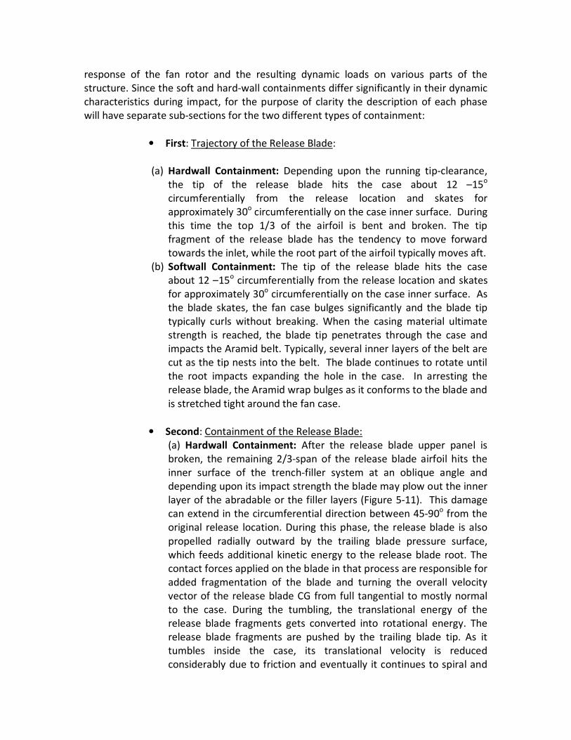
response of the fan rotor and the resulting dynamic loads on various parts of the

structure. Since the soft and hard-wall containments differ significantly in their dynamic

characteristics during impact, for the purpose of clarity the description of each phase

will have separate sub-sections for the two different types of containment:

• First: Trajectory of the Release Blade:

(a) Hardwall Containment: Depending upon the running tip-clearance,

the tip of the release blade hits the case about 12 –15o

circumferentially from the release location and skates for

approximately 30o circumferentially on the case inner surface. During

this time the top 1/3 of the airfoil is bent and broken. The tip

fragment of the release blade has the tendency to move forward

towards the inlet, while the root part of the airfoil typically moves aft.

(b) Softwall Containment: The tip of the release blade hits the case

about 12 –15o circumferentially from the release location and skates

for approximately 30o circumferentially on the case inner surface. As

the blade skates, the fan case bulges significantly and the blade tip

typically curls without breaking. When the casing material ultimate

strength is reached, the blade tip penetrates through the case and

impacts the Aramid belt. Typically, several inner layers of the belt are

cut as the tip nests into the belt. The blade continues to rotate until

the root impacts expanding the hole in the case. In arresting the

release blade, the Aramid wrap bulges as it conforms to the blade and

is stretched tight around the fan case.

• Second: Containment of the Release Blade:

(a) Hardwall Containment: After the release blade upper panel is

broken, the remaining 2/3-span of the release blade airfoil hits the

inner surface of the trench-filler system at an oblique angle and

depending upon its impact strength the blade may plow out the inner

layer of the abradable or the filler layers (Figure 5-11). This damage

can extend in the circumferential direction between 45-90o from the

original release location. During this phase, the release blade is also

propelled radially outward by the trailing blade pressure surface,

which feeds additional kinetic energy to the release blade root. The

contact forces applied on the blade in that process are responsible for

added fragmentation of the blade and turning the overall velocity

vector of the release blade CG from full tangential to mostly normal

to the case. During the tumbling, the translational energy of the

release blade fragments gets converted into rotational energy. The

release blade fragments are pushed by the trailing blade tip. As it

tumbles inside the case, its translational velocity is reduced

considerably due to friction and eventually it continues to spiral and

slide with low rotational velocity until it may come to rest by hitting

some other barrier in its path. The containment case will bulge in the

region of impact damage but will not be punctured.

(b) Softwall Containment: In this type of containment the blade

fragmentation is very minimal, with majority of the blade remaining

almost intact. The release blade tip starts curling in the direction of

rotation as it skates on the case. In metal blades, most of the

deformation of the release blade limited to bending and twisting of

the airfoil without any significant size metal debris being liberated.

The release blade is impacted by the trail blade and is forced radially

outward, punching the release blade through the casing shell. The tip

of the release blade is caught in the Aramid belt and may cut-through

the inner layers of the Aramid wrap (Figure 5-12). This damage forms

a local sack-line bulge in the wrap and in a contained event eventually

brings the release blade to a complete stop.

• Third: Fragmentation of the Release Blade :

(a) Hardwall Containment: In the hardwall containment, the blade

usually fragments in three pieces. The top 1/3 typically separates in

one piece, the mid-section in another smaller piece, and the bottom

(root) piece is usually the heaviest and largest.

(b) Softwall Containment: In the soft-wall containment, the release

blade fragmentation is minimal and typically the majority of the blade

remains intact. Metal blades typically have adequate plastic ductility

to allow the majority of the tip to curl. It is not unusual to have minor

fragmentation of the lead or trail edges as the blade punches a hole

in the inner shell and then imbeds in the Aramid wraps.

• Fourth: Rotordynamic Response during the safe shut-down period:

Following blade release, the unbalance force drives the heavy side of

the fan rotor off-center. This causes the tips of the undamaged heavy

side blades to start rubbing against the fan case. The rub digs out rub

strip material and causes the fan rotor to slow down and start orbiting.

During this phase, the containment structure (fan case) starts

responding dynamically to the rotating unbalance load vector. The

resulting response is essentially the superposition of the decaying

response from the first three phases of impact loading with the

imbalance driven forced response during rotor run-down. This phase

of the FBO event continues until the engine has been shut-down and

the fan-rotor has slowed to a speed that does not create significant

unbalance response.

• Fifth: Wind-milling or Rotordynamic Response due to Sustained

Engine Imbalance: This phase of the FBO event occurs after the safe

shut-down of the engine (15 seconds for the pilot to initiate shut-

down, plus the engine run-down time) and relates to steady-state low-

speed windmilling as the aircraft is flown home. Although the engine

has sustained significant damage, the aerodynamic forces acting on

the fan are typically more than adequate to prevent rotor seizure. The

asymmetric rotor damage resulting from an FBO event equates to a

very large imbalance, which even at low rotor speeds (i.e. 10-20% of

the maximum permissible speed) can generate high unbalance loads.

During this phase, the fan-blade tips may intermittently rub against

the containment-case as the fan and full LP-rotor orbit with large

amplitude [23].

The complex dynamic response of the FBO event must be accurately captured in an

analytical model used for FAA certification such that the following certification

requirements can be assessed:

(1) Containment

(2) Mount Evaluation

(3) Fire Evaluation

(4) Safe operation of Aircraft level Assessment due to engine windmilling

unbalance loads.

Details germane to each specific engine design will determine the specific details for

how a release blade interacts with the case, to what degree the case may be holed, and

to what degree fragmentation of trailing blades may occur. Therefore the forgone

discussion of the generic FBO event is provided as an example of how a generic engine

design may act during a blade-out event. Not all designs will behave similarly so the

applicant must carefully assess how the details of their design influence the FBO event.

5.7.3 Current State of FBO Simulation & Historical Perspective of Non-linear Analytical

Dynamics Advancements

Early engine rotor and structural dynamics analyses were limited by available computing

capability and therefore centered on natural frequency analysis and frequency domain

rotor forced response analysis. Until the mid-70’s almost every frequency domain forced

response of any realistic dynamical system was based on linear theory and transient

response analysis was typically analyzed in modal space using only the first few

fundamental modes of rotor vibration. The dynamic response of non-linear systems was

limited in the frequency-domain and time-domain calculations were not often

attempted due to numerical instability associated with forward-marching solutions.

Time-domain transient response calculations for non-linear systems, especially when

subjected to impulse excitations, were especially difficult to handle because of

numerical stability issue caused by the need to vary the time-step size, t. For transients

of interest to the FBO problem, the time-step size could easily be in the range of 1.E-8

seconds, and that makes the solution of real-life problems beyond the capabilities of

even the fastest computers of the early seventies.

To address the numerical difficulties experienced with early explicit time marching

methods, implicit methods, such as Newmark’s ββββ -method, were developed to allow

stable integration with larger time steps. Unfortunately, for high-speed blade release

problems, the large time-step size was unable to accurately capture the very rapid

contact-impact changes typical of these events. With the introduction of faster

computers, as well as advancement in numerical algorithms, explicit time-integration

techniques were becoming feasible for high-speed events with rapidly changing contact-

impact dynamics. By the late 70’s, the first such code DYNA3D, developed by John

Hallquist [24] at the Lawrence Livermore Laboratory, was made available in the public

domain. Since then, Hallquist has continued private development and the result today

is LS-DYNA. In 1983, Stallone and his colleagues [25] used the code TETRA to be the first

to compute the time-domain transient response of a fan rotor to a fan blade-out event.

During this period, every major commercial aircraft engine manufacturer was

developing their own proprietary versions of in-house transient codes to analyze

different aspects of the typical Engine FBO event.

Although much proprietary work was ongoing at the major aircraft engine

manufacturers, the first publically documented application of an explicit-integration

technique to analyze the combined effect of fan blade-loss and resulting unbalance

response on the transient behavior of a real LP-rotor system was documented by Cosme

and his coworkers [34], which used a code called Plexus. Although a significant step

forward, the Cosme model was limited to only 4 blades (1 release and 3 trailing blades)

on the rotor. In 2006, Shmotin [26] et al were the first ones to publically report the

successful application of LS-DYNA to simulate a turbo-fan engine Fan blade-out event.

Although another step forward, the Shmotin model considered only a sector of the fan-

rotor containing only 6 blades (Figure 5-13).

Proprietary development at the engine manufacturers has continued and today it is

informally reported, though not documented in the public literature, that each has

developed at least some capability to perform full engine transient simulation using LS-

DYNA. This proprietary capability has been reported to be part of work each engine

manufacturer goes through in preparation for major certification tests, such as FBO,

icing and bird strike. Without this capability to vet their designs, many manufacturers

likely would not pass these key tests on the first attempt.

Until now, LS-DYNA has been used by all major engine manufacturers as an analysis tool

at appropriate stages of their design process where one or more of their engine

components gets subjected to a significant transient dynamic loading. The extent of

usage of LS-DYNA for FBO simulation may vary among the various engine manufacturers

depending upon their respective in-house expertise in using the code. Historically LS-

DYNA has been used in a supporting role to determine readiness to perform a full

engine test, or in the engine certification process to generate the release blade impact

loads subsequently used as an input for the detailed analysis of mount-system loads in

NASTRAN, or when allowed by the regulatory agencies as a tool to assess design fine

tuning following a FBO test.

The LS-DYNA modeling of a FBO event on a fully-bladed fan rotor capturing both the

release blade impact phase as well as the rotordynamic response phase for an entire jet

engine has only recently been discussed in an open published literature by Sinha and

Dorbala [22]. As a further discussion of the full-engine modeling process, one must

introduce some of the acronyms, commonly used in turbo-machinery industry, such as

LPT for low-pressure turbine, HPT for high-pressure turbine, HPC for high-pressure

compressor and LPC for low-pressure compressor or booster, respectively. These

components and their contribution to the post-FBO dynamic loads to various parts of

the engine structure and the mounting system and their analytically determined safe

design margins are key to the success of any FBO analytical simulation. The details of

this approach are discussed in Section 5.7.4.2. This detailed LS-DYNA model provides

information about the critical pieces of dynamic response of the engine such as fan disk-

orbit, bearing load time-history and other accessory characteristics as well.

(1) In the LS-DYNA simulation of a fan blade-out event, the recent practice in the

public domain published literature (Shmotin et al 2006) has been to model only 180-

degrees sector of the external casing structure. This simplified model produces

reasonably good results about the impact resistance capability of the containment

structure as well as the release blade fragmentation under primary impact. In this

approach, one usually considers only the three blades representation of the fan rotor

and a 180-degrees sector of the fan casing. The finite-element mesh contains a partial

sector of the fan shaft and disk segment with sufficiently fine details of the blade

geometry as presented by Shmotin [26] and is also discussed in this document in more

detail later on under Section 5.7.4.1. However, the fact also must be recognized that a

sector model is never an adequate model for analyzing the rotor-dynamic characteristics

and the resulting dynamic response of the entire system. For determining the unbalance

response of the fan rotor it is necessary that the transient analytical simulation be

carried out for several revolutions of the LP (low pressure) shaft. For this analysis phase,

one needs the fully bladed rotor including the LPT shaft and disks for simulating the FBO

event in LS-DYNA and one should run it for a sufficient length of time with a normal

termination so that the rotor response due to unbalance forces can be fully investigated.

The size of these models varies with engine size and complexity, but in general are fairly

large, consisting typically of at least a million nodes (Figure 5.10) and a half million

elements. Rather than try to set limits on size, the critical issue to ensure the model has

adequate nodes and elements to accurately simulate the actual FBO event as close as

possible. The biggest challenge in any long-running LS-DYNA simulations (40 – 100 ms

event simulation range) is to obtain a time-domain solution without encountering

numerical instability. The basic workhorse of the LS-DYNA finite-element meshing

scheme is a constant-strain 8-noded brick element. However, due to the reduced

number of integration points, these brick elements are prone to hourglass instability, a

type of numerical instability seen when mesh resolution is not high enough to

accommodate the applied loading. This propensity to have hourglass issues is a result of

the explicit integration scheme and causes additional complexities when running LS-

DYNA simulations.

(2) The other certification scenario where LS-DYNA has successfully been used to

evaluate the design margin of individual critical components or accessories attached to

the engine casing. In this application, a fine-mesh model of the particular component

and key attachment engine case structure is constructed. Velocity boundary conditions

in the form of a time-history from a previously generated NASTRAN transient run-down

analysis, or response data from a previous applicable engine test, are applied as the

external forcing function to the case structure part of the model. The LS-DYNA results of

a sub-model for a particular component provide much better detailed information

about the transient state of stress and plastic strains in critical areas of the component,

that may not be possible in a large-size full-engine NASTRAN model.

5.7.4 Modeling Considerations in LS-DYNA

The main purpose of this document, as outlined in Section 5.7, is to eventually eliminate

the need for a full engine fan blade-out (FBO) test by an equivalent LS-DYNA analysis.

Thus, it is necessary to discuss as to how in today’s process a typical engine FBO test

would be done and how the results and the data collected during the test are used in

the certification process to meet the requirements of FAR 33.94 and FAR 25 with the

aircraft manufacturer. The FBO engine test, required to demonstrate the compliance

with FAR 33.94, is typically run with the engine mounted on a test stand at the engine

manufacturer’s facility. To demonstrate compliance with the regulations FAR 33.23

(Engine Mounting Attachments and Structures), the mount evaluation needs to assess

the loads imposed on, or transferred to the engine mounts and the associated vibratory

response of the engine. In this process, the current practice is to run the NASTRAN

analysis in two steps:

(a) First phase of analysis involves duplicating the test-stand condition in order to

validate the analytical model prediction against the FAR 33.94 FBO test requirements.

(b) Afterwards for FAR 25 requirements, the second phase of analysis involves to

exercise the engine model with the process and the modeling assumptions developed

and validated under item-(a), which in the second phase of analysis also includes the

wing and the pylon of the aircraft to generate the FBO loads.

5.7.4.1 Process of Developing a Validated LS-DYNA Model

It should be obvious that if the engine certification has to be obtained through a stand-

alone transient dynamic analysis, then the above step-(a) would be replaced by an

equivalent LS-DYNA modeling, the accuracy and the dynamic characteristics of which

must be validated before this model can be exercised and can be used for generating

loads. For a generic two shafts turbo-fan engine, the LS-DYNA model will have 4 major

assemblies viz.

(1) Static Structure (detailed list of components outlined in Section 5.7.4.2)

(2) Rotor-1 (LP rotor comprising of Spinner cone, Fan, booster and LPT with mid-

shaft disk and blades)

(3) Rotor-2 (HP rotor comprising of HPC, HPT with disk and blades)

(4) Test stand and Engine mounting and attachment system to hang the engine.

It should be recognized that the above list is a very broad classification of major

assemblies. In an actual engine, each of these major components may have hundreds of

other smaller parts, which need to be modeled correctly in LS-DYNA. The accuracy of

the LS-DYNA modeling should be determined and documented based as a minimum

upon the following list of criteria:

(a) Geometrical details such as size, shape, thickness (usually gets transferred

directly from the engineering drawing)

(b) Material data such as density, Young’ modulus, Yield strength etc at

operating temperatures for each components.

(c) Interfaces and clearances (How each component is component is connected

or is transferring load to the adjacent component)

(d) Static loads applied to the engine structure, and measuring displacement and

clearances at different turbo-machinery stages.

(e) Modal test of the bolted hardware such as inlet, exhaust centerbody, and

exhaust nozzle.

(f) Dynamic characteristics of each component in terms of its natural

frequencies in free-free condition, and the assembled LP and HP rotors.

(g) Forced response from unbalance testing of the assembled LP and HP rotors.

(h) Modal test of test stand and also documenting the dynamic characteristics of

the rig, if a rig test is planned in support of certification process.

(i) Modal test of fully assembled engine for N=1 ( 1 diametral response).

Only when each component’s finite-element mesh has been individually verified for its

accuracy based upon the above list of criteria, it can be used in the assembly to

generate the LS-DYNA model involving 4 major assemblies, viz. Stator, Rotor-1, Rotor-2,

and the Test stand.

5.7.4.2 Types of Analyses in LS-DYNA

For rapid turn-around of preliminary development study models, the fan blade

containment structure capability can be analyzed using a 180-degrees sector of the fan

case. When using the half model to assess initial containment capability, only three

blades are usually required. Depending on the complexity of the casing structure and

available computing power, the analyst may opt to perform the initial containment

analysis with a full 360-degree containment structure model and three bladed fan

model. Regardless of the model used for initial containment design assessment, once

the preliminary configuration is worked out, a fully bladed 360-degree model is used to

look at additional revolutions and provide insight into follow-on damage. From the LS-

DYNA modeling perspective, the first 3 phases of the FBO event are commonly

simulated using a detailed 3-blade model, while the rotordynamic response of the LP-

shaft, described earlier in Section 5.7.2 are best simulated using a full-bladed rotor

model:

(a) Blade Containment analysis (3-blade model)

(b) Dynamic Response of the Fan Rotor analysis (fully-bladed rotor model)

The initial blade containment event, item-(a) in the above classification, falls into the

discipline of impact analysis dealing with the release blade as the projectile and the

containment shell as the target. This modeling approach is best suited for the engine

manufacturer's internal design process and is focused on evaluating the various

containment design options. An efficient use of this relatively quick turn-around LS-

DYNA model may help in meeting the engine manufacturer’s internal requirements for

assessing basic containment before making the first attempt at the containment test,

but it is not adequate for assessing dynamic loads. The continued rotation analysis,

item-(b), is a rotor dynamics problem, in which the dynamic response of the fan rotor

and its interaction with the containment structure through the rub blades are the main

focus of attention. The detailed geometrical representation of key engine components

and their connection to each other in terms of rotors, shafts, bearing support structure,

structural casings, mounts, brackets, bolted-joints and v-groove interactions in the LS-

DYNA simulation are key to the accurate prediction of analytically generated dynamic

loads.

Since a key part of the FBO requirement is demonstration of engine mount integrity, the

FBO full engine model must include a detailed representation of the forward and aft

mount systems, including representation of the strut or pylon dynamics. This is required

so that the analytical model is able to accurately demonstrate that after the FBO

containment event, the mount system would be able to withstand the resulting large

dynamic loads without detaching itself from the aircraft support structure.

The fire evaluation generally focuses on the loads, deflection, and vibratory response of

components that carry flammable fluids, such as fuel lines, oil lines, oil tanks, gearboxes,

fuel pumps and lube pumps. If analysis demonstrates that the proposed design

change(s) to the engine would not increase the loads and dynamic response of these

components, or damage the capability of these components due to large plastic

deformation or impact against adjoining components, then a combination of

component analysis and similarity might be used to validate these components.

However, if the loads and responses are increased, or the capability of any component is

reduced by the design change, then further evaluation of any adversely affected

component’s capability must be conducted to show the component(s) will not fail or

catch fire. Possible approaches include:

1. Oil & fuel carrying tubes and hoses will not rupture and release flammable fluid.

One could include all components in the full LS-DYNA, but this is not typically a

practical approach. Alternatively, one could use a sub-model as described

previously in Section 5.7.3 to predict the tube deflections and evaluate the

critical component stresses.

2. Controls & accessories that contain fuel & oil will not impact or be impacted by

surrounding hardware resulting in failure or leakage of flammable fluid. This is a

large deflection concern and needs to be based on the full model analysis. One

approach might be to use simplified representation of these accessories in the

model, then take the component translations and rotations back into the 3-D

CAD program to assess whether extended component features will interfere.

As discussed earlier, during the impact phase of the FBO event, the release blade acts

like an oblique impactor having both rotational as well as translational kinetic energy

and the outer casing or the containment structure acts like a target. In the following

paragraphs, first we will discuss the fan case modeling strategies and later on blade

modeling considerations.

5.7.4.3 Fan Blade Modeling Considerations

The initial impact of the release blade initiates a sequence of very complex high-speed

contact-impact events outlined in Section 5.7.2, and this initial impact must be captured

very precisely in order to predict the ensuing transient dynamic loads correctly. To do

this accurately, a blade mesh must contain adequate detail to represent the blade

aerodynamic shape and the pre-release steady-state stress-field. If the blade steady

state stress field and resulting geometry is is not initialized accurately, the blade model

will undergo undue elastic oscillations during the initial explicit time steps. To prevent

this numerical problem, the analyst must take into account such effects as blade stagger,

lean and airfoil twist when applying centrifugal stress-stiffening. If the steady-state

operation deformed shape of the blade airfoil has been determined correctly, then

appropriate convergence criteria applied during the initial implicit solution time steps

will verify the initialization.

5.7.4.4 Fan Case Modeling Considerations

The fan case, in general, is an axi-symmetric cylindrical or slightly conical structure with

the typical cross-sections shown in Figure 5.11 for a hard-wall or Figure 5.12 soft-wall

designs, respectively. In the 180-degrees simulation approach, the two ends of the

containment shell may be considered as sitting on roller supports. The impact force of

the release blade on the hard-wall case deforms the containment structure making a

visible plastic bulge in the metal fan case. In general, the magnitude of this force is also

large enough to remove the abradable or any other trench-filler material in the vicinity

of the initial impact. As the released blade continues along its trajectory, it continues to

remove any abradable or trench filler material that comes in its path. The mesh density

of the outer fan case as well as the trench filler material, both in the thickness as well as

in the circumferential directions, must be fine enough to capture the local removal of

material and properly predict the bulge in the metal hard-wall casing. Depending upon

the engine manufacturer design philosophy or application design requirements, some

fan case designs may have a horizontal split line or case access port. In evaluating the

containment capability of casing designs with a horizontal split-line or access port, it is

extremely important to ensure that during the release-blade impact the flanges at the

split-line, or port, do not separate in such a way that the blade or its fragments may exit.

Hence, the LS-DYNA model must accurately include the structural details of any joints in

the case so that the model is capable of capturing any local weakness.

The soft-wall case with Aramid material wrap requires some very special material

models in LS-DYNA if it is to capture the release-blade impact event, the local bulging of

Aramid yarn, and the dynamic response of the woven-fabric. The modeling

considerations for such casing designs have been discussed in much detail by Bansal and

his coworkers [21].

The above discussion of modeling the fan casing structure is mainly driven by the need

to correctly capture the physics of the initial impact event and accurately evaluate the

containment capability of the structure. In this event, the release blade behaves like an

impactor and the containment shell with Aramid wrap is the target. As noted earlier, the

rotordynamic response during the engine shut-down, as well as during the subsequent

low-speed windmilling fly-home condition, involves rotor-casing system dynamics

analysis that must accurately capture fan blade tip-rub interaction with the fan case and

the resulting system response. The fan rub against the casing is influenced by the

condition of the abradable and trench filler. If the initial blade release plows out an arc

of abradable and filler, then the fan will experience intermittent rubs. If the trench filler

is plowed out around 360-degrees, but the imbalanced eccentricity is greater than the

filler depth, then the fan will rub around the full circumference of the case. These types

of rotor-stator interaction should be captured by the LS-DYNA model and may exhibit

sub-synchronous response [23]. An intermittent rub makes the dynamical system highly

non-linear, which can create jump discontinuities in the dynamic response. The casing

model to be used for predicting the dynamic response [36] during additional revolutions

of the fan rotor should also include all the different accessories hanging from the casing

such as Gear box, oil tank, fuel measuring unit (FMU's), etc. The prime requirement for

an acceptable engine casing model is that it should be able to predict the correct

dynamic load transfer from the bearing supports [46, 48] through the engine case to the

engine mounts. This model needs to account for the fan blade interaction [41, 42, 43,

49, 50] during subsequent revolutions. For correct load transfer from the casing to the

inlet or to the aft-fan case, the modeling of bolted joints poses unique challenges [28].

5.7.4.4.1 Partial Sector Analysis for Containment Evaluation

This is a relatively simple and quick way to analytically simulate the impact phase of an

FBO event, however, it has a very limited use in terms of a thorough analysis needed to

evaluate the containment capability correctly. For an experienced user of LS-DYNA, it

may be used as a good screening tool for evaluating various containment options.

However, due to imposed constraints at the cut-boundaries of the casing such a model

can very well miss the asymmetric response such as likelihood of developing a

circumferential crack in the inner shell and running into the softwall containment

system. Due to these shortcomings, the use of half model is not recommended to

resolve any engine certification related issues. So far the transient dynamic loads

through the containment structure is concerned, the magnitude of peak loads predicted

by the half casing-model will not be considered as an acceptable piece of data by FAA.

In this approach from the rotor side, one models only a small sector of the fan-rotor

with few blades (Figures 5.13 and 5.14) separated in the circumferential direction by an

angle determined by using the following formula:

Circumferential separation in degrees = ( 360o) / (Number of fan blades on the rotor)

Figure 5.13 A 90-degree sector of the fan rotor model used by Shmotin’s et al [26].

The ends of the 180-degrees sector of the fan case may be considered sitting on roller

supports. A recent AIAA paper by Shmotin and his coworkers [26] presents a good

description of this modeling approach (Figure 5.13) in LS-DYNA. The blades as well as

the fan containment structure are modeled in sufficient details using 8-noded brick

elements called *ELEMENT_SOLID. This being a constant strain element, one must use a

minimum of 3 elements-thru-the-thickness everywhere. The blades are rotated about

the engine axis using *BOUNDARY_PRESCRIBED_MOTION_NODE for the root nodes and

*INITIAL_VELOCITY_NODE for all other nodes. It is recommended that ahead of the LS-

DYNA transient analysis, the stress initialization for the rotating blades must be done

using an implicit code such as ANSYS or the implicit version of LS-DYNA itself. All the

inner surfaces of the containment surface as well as any other filler material surfaces

should be specified in separate sets of *SET_SEGMENT (segments have to assume no

failure). The contact interface between the blades and inner surfaces of the fan case

must be defined by using *CONTACT_ERODING_NODES_TO_SURFACE. Furthermore, it is

imperative that due to very-high strain rates involved in these simulations, one uses

strain-rate dependent properties whenever they are available. One good resource in

public domain for high-strain-rate properties of typical aerospace materials is the report

by Nicholas [27] written in 1980. The material model both for blades as well as fan

casing could be either,

(a) *MAT_STRAIN_RATE_DEPENDENT_PLASTICITY

(b) *MAT_PIECEWISE_LINEAR_PLASTICITY

Separate material models are also being investigated by NASA. There may be some

other specific material models of proprietary nature, which have been developed by

various engine manufacturers for their own in-house usage. It must be pointed out that

results of LS-DYNA half-model of the casing should be limited to preliminary design

evaluate evaluation of containment concepts only, and is not recommended for any

certification purposes. The 360-degrees fan casing model used by Cosme [34] (Figure

5.14) has many features which 180-degrees half model will not be able to highlight. For

this reason, a 3-blade sector model of the rotor and a 360-degrees model of the fan

casing can very well be used to assess the initial containment capability of the design.

Figure 5.14 A partial rotor sector model used with 360-degrees case by Cosme [34]

All the material models in LS-DYNA must be used with FAILURE –option “ON”. During

the design phase, one may want to assess the margin to failure while designing for

success. One does not have to use any specific hourglass control parameter or, a

Penalty-factor other than the default values built-in the code already. If the LS-DYNA

results indicate the presence of hourglassing instability, it is best handled by making the

mesh finer, rather using different types of hourglassing parameter. The remeshing

should be done in such a way that,

(a) Point load situation during the entire duration of the transient analysis is

eliminated by moving to finer mesh option, such that a concentrated load is

always shared by multiple surrounding nodes.

(b) Slave side segments are finer than the Master side segments.

(c) The mesh is fine enough so that for a given nodal velocity and computed t,

the deformed element does not turn inside out.

The above condition is not a requirement rather simply a guide line in an attempt to

keep the mesh size manageable, and to be able to capture the right physics of the initial

FBO containment event. If the mesh has already been generated, then one can achieve

a similar objective by setting a smaller time-step scale factor as well.

In this modeling approach, it is not necessary to consider the gas loads or transient

thermal gradients in the analysis because the blade release/containment has finished

before the engine has time to surge. Since, the release blade tip fragments often have a

tendency to go forward, and since the gross deformation at the blade impact location

typically involves distortion of the inlet attachment flange, it is necessary to include the

inlet in this simulation. Similarly, key adjacent hardware at the AFT-end of the

containment structure needs to be included in the analytical simulation. Depending

upon the requirements, one may either model the bolts and the bolt-holes in the

flanges explicitly [28] or, one can also use *CONTACT_SURFACE_TO_SURFACE interface

definition. The modeling of other engine components such as thrust links, thrust

reversers, turbine rear frame etc play an important role in determining the system

dynamic response of the entire engine following the initial FBO event.

5.7.4.4.2 Soft-Wall Containment (Kevlar) LS-DYNA Modeling Considerations

In 1989, Leech and Abood were among the first to discuss the finite-element modeling

issues associated with woven fabric construction [29] materials such as Kevlar and

especially its dynamic response to impact type of loading. The modeling technique to

capture the true physics of woven-fabric behavior during high-velocity impact is a topic

of current on-going intensive research in academia and industry. To date, the modeling

techniques for woven fabrics have yet to reach a matured state for generic application

thus these models must be validated empirically for each general application so that

they can be applied in the LS-DYNA simulation of the Fan blade-out containment [20,21]

(Figure 5.15). In modeling fabric containment belts, the fabric elements should be able

to capture the response associated with crimp action of the yarn cross-over. These soft-

wall containment systems are able to absorb and dissipate the majority of the kinetic

energy of the release blade through large local deformation of the fabric belt, without

causing significant fragmentation of the release blade.

Figure 5.15 180-degree sector Kevlar fan case with 2 blades of used by Bansal et al [21].

5.7.4.4.3 Hard-Wall Containment Modeling and Fragmentation of the Release Blade

In hard-wall containment, the majority of the release blade kinteic energy is absorbed

and dissipated through large plastic deformation of the casing and significant blade

fragmentation as it tumbles inside the casing. Since the blade is not allowed to

puncture the hard-wall case, a considerable amount of dynamic load-sharing with the

case can take place during the 15 second run-on allowed before engine shut-down.

5.7.4.5 Combined Dynamic Response of the Engine due to Impact and Unbalance

Forces

When the dynamic response of the rotor-casing system is important, one needs the

fully-bladed rotor including the LPT rotor and disk for simulating the FBO event in LS-

DYNA. This model must be run for a sufficient length of time (usually 50 – 100 ms) to

capture the system response due to unbalance forces [22, 23, 34, 35]. These models

require a large number of nodes and elements in order to accurately simulate all the

important aspects of the full FBO event. It must be noted that after the initial impact

from the release blade, the large fan unbalance force affects the loads in the entire

engine structure, pylon, and wing, as the dynamic loads propagate through the system.

5.7.4.5.1 Details of the Rotor and Bearing Modeling

The typical gas turbine engine consists of two or three concentric rotors. For this

discussion, the focus will be on the dual-rotor configuration consisting of a fan-LPC-LPT

rotor (Figure 5-16a) as the inner rotor and HPC-HPT rotor (Figure 5-16b) as the outer

rotor.

Bearings connect the rotating shafts to the stationary casing, and sometimes bearings

are located between rotating shafts. A typical gas turbine engines may use following

types of bearings:

(a) Ball bearing (axial and radial loads),

(b) Roller bearing (radial load) only, and

(c) Tapered roller bearing (axial and radial loads).

Modeling the bearing interface between the rotating shaft and the stationary casing is

an important part of constructing an accurate engine model. Bearings can be simulated

in a number of ways in LS-DYNA, one approach applicable to both types of is to use the

*CONTACT_NODE_TO_SURFACE type of interface. The stator side of the ball bearing is

represented by a U-shape groove for the rotor side elements to be sitting inside two

axial walls preventing its axial movement and providing rotational stiffness to withstand

the bending moment. On the other hand, the stator side of the roller bearing is

represented by a cylindrical surface, such that the rotor side elements are free to move

axially.

During high energy portions of the FBO events, the concentric shafts may rub so it is

necessary that this type of model be capable of capturing the deformation in the shafts

leading up to and including the relative rubbing of concentric rotating shafts. In order to

capture this accurately, the shafts must be modeled with shell or solid elements, since

beam elements do not allow the appropriate relative motion nor ability to capture

continuous or intermittent rubs.

Blades, other than the fan blades, can be modeled using shell elements with the

*ELEMENT_SHELL_OPTION. It is very important, from the dynamic results accuracy

point of view, that individual blades on both rotors be modeled in such a way that their

deformation due to rubs or clashing with any stator components are properly captured

in the LS-DYNA model. Disks are usually represented by 8-noded brick elements due to

the typical geometries of these parts. It should be pointed out that one must follow a

geometrically correct procedure for mating 6-degree of freedom shell nodes (i.e. blades)

with the 3-degrees of freedom nodes on brick elements. They can also be connected

using *CONSTRAINED_SHELL_TO_SOLID

Figure 5.16a A typical Fan-LPT rotor Figure 5.16b A typical HPC-HPT rotor

Figure 5.16 LS-DYNA model of the two concentric rotors used by Sinha and Dorbala [22].

5.7.4.5.2 Details of the Engine Mounts and Supporting Structure

Current FAR 33.94 FBO test is typically run with the engine mounted to a test stand at

the manufacturer’s facility. In addition to the validated engine model developed earlier,

the first phase of the analytical model should include the following:

(a) Engine mounts (both forward and aft mounts based upon production

drawing)

(b) Production aircraft pylon

(c) Test facility adapters that connect to the pylon test-stand.

The above engine/support structure model would then be run to demonstrate that the

engine is capable of meeting the engine level requirements in FAR 33.94. To develop

the aircraft level installation design loads, the engine model is removed from the test

stand and attached to the aircraft model. The aircraft model typically includes:

(a) For under-wing installations: aircraft pylon, and wing grounded at the

attachment to the fuselage, or a full aircraft model (structure away

from the wing attachment may be a beam model). The transient

dynamic loads during FBO are generated for various fuel levels and

fan blade release angles. The range of release angles determines

sensitivity of components, while the fuel loads change the distributed

mass of the wing which affects the system dynamic response and

resulting design loads for the engine mounts.

(b) For fuselage mounted installations: the model includes the aircraft

pylon, at least 1 plug of the aircraft fuselage (containing the pylon

attachments to the primary airframe structure), and either a 3-D or a

beam representation of the remaining aircraft.

Mount loads have been shown sensitive to release angles, fuel levels (wing mount) and

installation parameter (Left hand and Right hand engine installations). Therefore in a

typical analysis the design loads may be calculated for:

(a) 8 fan blade release angles

(b) 2 - 3 different fuel levels

- In twin-engine aircraft applications: Left and Right hand side release

condition.

- In 4-engine aircraft applications: blade release on any of the four engines.

As mentioned earlier, the objective of the LS-DYNA analysis can be further extended to

generate the airplane certification loads. To do this, one would replace the test stand

support model with a model of the aircraft wing and the pylon. However it needs to be

noted, that most applicants end up running two models: one for the basic engine part

33 certification where the engine is mounted on the test stand; and a second for each

airplane specific part 25 certification where the specific airplane wing and pylon are

included. It is important to note that engine mount loads can be extremely sensitive to

the boundary conditions. For example, conducting the FBO analysis with a grounded

pylon will typically result in higher loads on the mounts than the engine model which

includes the flexibility of the aircraft wings in its support simulation. Since the blade

release angle may increase or decrease loading on various parts of the engine system, a

number of blade release angles are required to assess release angle effects. The

number of release angles may depend upon the engine configuration as well as past

experiences and the data of the aircraft manufacturer. The goal is to run enough

different blade release locations to capture the largest magnitude peak load in part of

the mount system. Typically, the different parts of the mount system will peak under

loadings from different release angles, so it is important to map out the peaks from all

conditions so that the mounts are capable of handling all release angles. In typical

engine hung from the wing of the aircraft, the number of release locations could be

anywhere between 8 to24. Thus based upon the forgone discussion, one can see that

for certification purposes, the applicant will need to generate mount loads covering a

range of conditions, which will be guided by the installation details.

The accurate representation of the aircraft wing can make the LS-DYNA model so large

in terms of total number of nodes and elements, that it may be almost impossible to

solve on any existing computer. For this reason, current practice is to use LS-DYNA

analysis for the part 33 test stand analysis, and then use other analysis methods for the

integrated engine-airframe analysis. With advances in computing capability and

numerical improvements in LS-DYNA modeling, these limitations are changing rapidly,

so it is conceivable that full system analyses in LS-DYNA may be feasible in the near

future.

The objective of the analysis should be to show that proposed changes to the engine do

not significantly modify mount loads relative to the baseline engine that was tested to

FAR 33-94. If the predicted derivative engine mount loads are higher than the baseline

test results, further evaluation should be conducted to show the mounts have sufficient

capability. If sufficient capability can not be demonstrated, or if the mount loads and

load distributions are significantly higher than the baseline engine test, or if the design

changes are so radical that the modeling capability falls into question, then a new FBO

engine test may be required to show compliance with FAR 33.94.

5.7.4.5.3 Details of Additional Non-Rotating Engine Structure and Attached

Accessories

In a typical full-engine model shown in Figure 5.17, it is obvious that in addition to the

fan containment ring (Section 5.7.4.1) one must also include the following critical stator

components in the LS-DYNA analytical model:

• Inlet

• OGV’s and Fan Frame

• Fan AFT-case

• Bearing housing

• Booster casing

• HPC Casing

• Combustor

• HPT Casing

• LPT Casing

• Thrust Links

• Exhaust Nozzle

• Exhaust Center Body

• All stator vanes

• Bypass Duct/Thrust Reverser

Most of these stator components are connected to each other by circumferential bolted

joints. In modeling bolted joints, one of the important considerations to predicting the

correct joint stiffness is to correctly simulate the effect of pre-tension in the bolt shank.

In LS-DYNA simulation this can easily be included by using *INITIAL_STRESS_SECTION

and *DATABASE_CROSS_SECTION_PLANE_ID commands in the input deck.

Figure 5-17 A full-engine LS-DYNA model reported by Sinha and Dorbala

[22].

Figure 5-18 Key locations of the engine with structural bolted joints reported by

Czachor [28].

Czachor’s paper [28] provides an excellent description of all the major structural bolted

joints in an engine (Figure 5-18). In order to accurately predict the rapidly changing

dynamic loads coursing through the engine during the aftermath of an FBO event, it is

important to model these bolted joints correctly. In addition to the major bolted joints,

it must be noted that the following circumferential structural connections are not bolted

but do transfer load and as such they exhibit more flexibility when transferring the load:

• Radial gaps between inlet, exhaust, cowling and reverser parts

• The V-groove joints at the forward and aft-end of the thrust reverser.

These non-bolted flexible joints in the circumferential direction have special features

such as:

(1) Radial compression only contact surfaces typically found between nacelle

components such as fan cowl to inlet and fan cowl to thrust reverser interfaces.

(2) Multi-directional compression only contact surfaces found at Thrust reverser V-

groove joints.

5.7.4.5.4 Analysis Considerations for Fire Evaluation and Limitations of Explicit

Technique

Other engine accessories such as the oil tank, auxiliary gear-box, fluid hoses and pipes,

pumps and fluid containing accessory components (generators, FMU, pumps, etc), may

be represented by individual rigid masses each rigidly attached to it’s associated

attachment flange. If any of these accessories becomes a fire concern due to possible

rupture of it’s casing or an attached fluid line (i.e. fuel, oil, or hydraulic), one may have

to include these items in reasonable detail as well. The current state-of-the-art is limited

to determining the peak dynamic stresses and actual deformation of the tubes and to

ensure that the peak values are within the allowable limits of the material.

Once the gross engine dynamic response has been established, local models of

accessories, gearbox, etc, can be constructed with appropriate volumetric detail and

driven with the attachment base motions from the full system model to determine local

loads, deflections, and dynamic interactions in these parts.

It should be noted that when assessing post-FBO response of the engine case and

accessory components, it is usually sufficient to model all the fan blades with a coarser

mesh representation than was described previously in item-(a) under 3-blade modeling

procedure for containment analysis.

5.7.5 Quality and Validity of LS-DYNA Analytical Results

As mentioned earlier, the major engine manufacturers have been using LS-DYNA

analyses in their internal design process to qualify the design of various components so

that they can successfully run the FBO test to demonstrate the FAR 33.94 compliance in

the very first attempt. The majority of best practices are based upon the lessons learned

and developed over the last decade by each engine manufacturer and therefore are

proprietary to the individual manufacturers. The use of LS-DYNA in lieu of an engine test

for certification is not an easy task and requires a highly skilled and experienced user

community with extensive technical background in transient dynamics and related

physics, as well as a corporate history of FBO test experience and the necessary data to

have developed and validated in-house best practices. This document has made an

attempt to compile publically available information published in technical journals as

well as the scattered pieces of other data available in public domain into one document

to assist an engine company with prior FBO test experience and LS-DYNA non-linear

transient analysis expertise to step up to applying LS-DYNA to certification of derivative

engine models by analysis. If in the future an engine manufacturer decides to follow

this route, then the actual FBO certification-by-analysis plan needs to be negotiated

with FAA and the extent of LS-DYNA modeling and supporting analyses for load

generation need to be established well in advance. In short, the approved certification

plan will set the ground rules for the accuracy and quality of LS-DYNA results, so that the

loads generated in this manner will be acceptable to the FAA for certification purposes.

The end use of the LS-DYNA analysis may determine the extent of modeling required, so

at this point one also must discuss as to the extent of the LS-DYNA simulation planned. If

the analysis is limited to simulating the initial impact event only as described as Phases I,

II and III in Section 5.7.2 for load determination purposes then 3-blade model might be

sufficient. However, in order to analytically demonstrate the requirements of the

conditions of 33.74, one must generate a fully-bladed fan-rotor model and should

include the FWD and AFT-mounts in the analysis.

To determine mount loads beyond the initial release (i.e. first several revolutions

beyond the initial release), a fully-bladed LP-rotor model is required for correct

predictions of FBO loads. As far the engine loads are concerned, one may include all

engine installation mounting and intermediate structure along with a part of the

aircraft-wing as well for better fidelity of dynamic results. Precise prediction of dynamic

loads, both in terms of magnitude and its time-history after an FBO event is very critical.

A correct LS-DYNA model of such a dynamic system should be able to predict the precise

timing of each key event during the FBO simulation.

The dynamic response of the LP-rotor during run-down (response as the engine

decelerates following shut-down from high power) has been of intense interest [35],

and several different approaches are being investigated on this front [34]. Most of these

approaches consist of some combination of partial-explicit and partial-implicit solutions.

The main challenges with an exclusively explicit solution, are associated with the general

shortcomings of any explicit-integration technique:

(a) Cumulative error due to truncation and round-off (This error can be

reduced by using the option for double precision executable of LS-DYNA).

(b) Hourglass instability in long-running solutions (This error can be reduced by

using some other specialized hourglass control options than the one built-in as

default option in LS-DYNA).

Although the ability to use LS-DYNA to accurately predict the run-down phase of an FBO

event although looks very promising, it does require further investigation. For the

rotordynamic analysis phase of the FBO event, all the axi-symmetric components going

through multiple rigid-body revolutions, such as shaft and fan disk etc should use

option-6 of the hourglassing parameters offered in LS-DYNA [36].

5.7.6 Transient Dynamic Response of the Rotor after Blade-Loss

As explained earlier in Section 5.7.1 following the initial FBO event, the entire engine

(rotor and the stator components) responds dynamically in a very non-linear fashion.

However, as the fan rotor is the main initiator and the driver of this highly non-linear

dynamic event, from the accuracy point of view it is important that the LS-DYNA model

of the fan-rotor must be able to capture some of the early key parameters of the LP-

rotor response such as the fan-rotor orbit and the bearing load time-history correctly. As

soon as a fan blade is released in a running engine, the LP rotor gets subjected to an

impulsive force (jolt) at the fan-disk acting radially outward on the heavy side of the

rotor due to introduction of sudden imbalance in the dynamical system.

5.7.6.1 Bearing Loads – Effect of Bearing Support Fusing

To reduce the transmission of fan imbalance loads to the engine case, some

manufacturers opt to fuse the structural support for the bearing closest to the fan disk.

The intent of the fuse is to release the bearing radial constraint and allow the severely

imbalanced fan to rotate about its mass center rather than being forced by a stiff

support to rotate about its original undamaged geometric center. This design approach

significantly reduces the imbalance force transmitted from a damaged rotor to the

engine casing. The technical basis for this design approach is presented in US Patent No.

7097413 titled “Bearing Support” [51].

The fused bearing system works in the following sequence of events. Immediately after

blade release, the resulting severe imbalance moves the fan rotor off-center from the

engine centerline axis. This causes a rapid and very severe increase in the load carried

by the bearing nearest the fan (usually called bearing number 1 because it is most

forward bearing in the engine). The severity of the load is usually controlled by the

magnitude of the imbalance and the extent to which the fan disk is cantilevered forward

of the number 1 bearing. When the load in the number 1 bearing reaches the design

critical load, the bearing support system fuses and the load path changes such that it is

transferred to the next bearing on the fan shaft. Without the support of the number 1

bearing, the fan is effectively soft supported on a longer cantilever than during normal

operation. This reduction in system stiffness and reduces the fundamental natural

frequency of the fan shaft.

In the rotordynamic analysis the focus is on the dynamic loads developing at various

bearing locations as well as the rub-loads being generated between the rotating blade

tips and the inner surface of the casing. The timing and magnitude of the peak bearing

load from the initial blade release is dependant upon whether the engine is configured

with a fused bearing. With the bearing fuse, the peak load typically occurs within the

first revolution following blade release. Without the fuse, the #1 bearing load may keep

increasing for 2-3 revolutions, ultimately peaking later and at a higher value than for the

fused configuration. It is very important when modeling to identify all the bearing

locations and support configurations before embarking on meshing because some

bearing by design may be capable of carrying moment loads, while others under

extreme rotation may be able to carry some moment load. In general, during the

extreme response of a FBO event a ball-bearing will take moment while most roller

bearings will not. The analyst should work with the engine bearing designer to

understand what loading might occur and then when checking model results verify the

predictions with the bearing designer to ensure the predicted bearing response makes

physical sense.

5.7.6.2 Fan Rotor Orbit

The accuracy of the dynamic load magnitude in an analytical model is directly related to

the model’s ability to predict the fan-rotor orbit correctly. The fan-rotor orbit following

the initial FBO event is directly dependent on the following 8 parameters:

(a) Abradable stiffness

(b) Containment trench-filler construction

(c) Total fan material loss and resulting unbalance due to secondary fan

impact damage

(d) Blade stiffness during rub

(e) Bearing Support stiffness (radial, axial, and moment)

(f) Blade Tip-clearance

(g) Shaft deformation

(h) Booster rub characteristics

It should be obvious that one needs to pay attention during the LS-DYNA modeling

phase to the accuracy and preciseness to which the above 6 parameters are

represented. As the rotor goes off-balance and its center of rotation starts moving; the

fan disk center starts orbiting in a spiral trajectory. As the radial eccentricity of the fan-

disk orbit increases, the tips of remaining fan blades may start rubbing as the running

tip-clearance is consumed. Since the containment structure tip clearance (clearance

after the abradable and trench filler are consumed) is a very important player in

determining the peak-magnitude of the dynamic loads being generated, it is very

important in the LS-DYNA meshing scheme that blade-tip clearances are accounted for

with sufficient accuracy [37].

5.7.6.3 Dynamic Loads due to Tips of the Fan Blades Rubbing Against the Case

After the fan disk orbit has become so large that the available blade tip running

clearances have been consumed, the blade tips start rubbing hard against the outer

structural casing. Once the blade tips make contact with the case, they generate a new

load path for transmission of the imbalance load. This load sharing across the fan

blades creates a very complex dynamic loading that requires careful modeling of the

blades and rub interface to predict accurately. The dynamic loads during tip-rub can

become so large that the blade tips may curl, blades may break, or rub-induced

vibration may occur in the airfoils. Care must be taken in modeling these events and the

engine manufacturer needs to have experience with adequately instrumented engine

tests to understand what kinds of phenomena are typical of his design approach.

It also need to be recognized that depending on fan tip, case structure, shaft flexibility,

and other factors, the fan rubs can be very local such that the blade might only be

rubbing on the lead-edge, mid-chord, or the trail-edge. In order to accurately predict the

peak magnitude of these tip-rub loads analytically using LS-DYNA, it is very important to

have a relatively very fine-mesh in the spanwise direction of the blades. These local

high-speed rubs can excite complex vibratory modes in the blade, such as the 2nd-stripe

chord-wise bending mode. Until recently, the trend has been to treat the fan blades as

rigid such that all the load being applied to the blade-tip is transferred to the disk-center

without any attenuation or magnification [38, 39], however, the flexibility in the fan

blade (Figure 5-19) plays a very important role coupling the blade motion with the rotor

deflection [40, 41].

Figure 5.19 LS-DYNA results showing dynamic nature of fan blade rubbing after the FBO

[22].

This is especially true both during the initial fan blade-out and also during the blade-

casing interaction [42], where both the flexibility of the blade as well as the dynamic

characteristics of the abradable surface may be extremely important. The eccentricity of

the LP-Rotor orbit after the FBO event, especially in engines with controlled fusing of

the Bearing # 1 support structure [51] is heavily dependent upon the abradable

behavior under dynamic conditions [50]. In the transient analysis results presented by

Legrand and Pierre [50] simulations one observes the extreme sensitivity to relatively

minor changes in abradable material parameters, such as:

(a) Abradable dynamic stiffness is highly non-linear (when comes in contact with

the fan blade-tip)

(b) Abradable density

(c) Damping characteristics of abradable ( Viscous vs. Coulomb’s frictional

damping)

In order to build confidence in the analytically produced results from a typical LS-DYNA

simulation, one needs to understand the dynamic behavior of abradable much better

than it is typically understood in today’s [31, 50] public literature. A new modeling

option called the SPH method in LS-DYNA has shown a lot of promise to capture the

right physics of minute amounts of material being removed as a result of the blade-tips

rubbing against the brittle material like abradable [32]. This method may provide to be a

step forward in accurate capture of fan-abradable rub modeling.

5.7.6.4 Dynamic Response of Engine Accessories

As mentioned earlier, the actual engine has many different accessories hanging from the

containment structure. The LS-DYNA model of the engine discussed in this document

should include accessories such as the Auxiliary Gear Box (AGB), Electronic Control Unit

(ECU – also known as the Electronic Engine Control, EEC, or Full Authority Digital

Electronic Control, FADEC), Fuel Measuring Unit (FMU), and oil tank, to name a few of

the common key accessories. Typically the metric of interest is the acceleration, in terms

of g’s, experienced at the center of gravity of the component and stresses in the

brackets retaining the component. Many of these components are mounted on rubber

isolators to absorb shock and reduce transmission of normal engine vibration to the

accessory. In modeling these designs it is important to accurately represent any non-

linear load deflection characteristics in the isolator. When the accessory contains

significant fluid and is susceptible to slosh loads, the fluid may be modeled in LS-DYNA

using the Null-hydrodynamic material option to simulate sloshing of liquids in cavities,

containers or fluid-filled tubes. The accuracy of the dynamic load generated due to

liquid sloshing inside these accessories may directly affect the outcome of the fire

evaluation.

5.7.6.5 Rubbing between Concentric Rotors

It should be noted that the clearance between concentric rotors (viz. LP-rotor and the

HP rotor) can be very tight in some parts of the engine. As a result, during the

extremely nonlinear dynamic response associated with an FBO event, rubbing may

occur between the rotors during the rotor dynamic phase of the response [36]. Since

the shafts are rotating at different speeds and sometimes in different directions, the

effect of a rub is to develop contact stresses on the sides of the contacting shafts. This

rubbing results in frictional forces that can create intense heat in the rub location

resulting in thermal distortion. Following an FBO event, usually rubbing between the

shafts [43, 44, 45] will be indicated by heat-generated discoloration of the metal. Again,

the engine manufacturer needs to have a historical experience base with prior FBO tests

in their generic family in order to ensure that derivative models are accurately capturing

the engine response.

5.7.7 Windmilling and Rotor Stability

As mentioned earlier it has been found that the newer high by-pass ratio turbofan

engines with wide-chord fan blades have a tendency to continue to rotate at a low rpm

even after safe shut-down. Even at low windmill speeds, the out-of-balance force

caused by a missing fan blade provides a significant source of excitation for the whole

engine-wing-aircraft structural assembly. This condition is referred to as `windmilling

imbalance' [15, 23]. Windmilling imbalance, though present in any damaged engine, is a

more significant phenomenon in high bypass turbofan engines where the magnitude of

the imbalance is higher and engines with fan bearing support fuses where the fan can

continue to orbit with high eccentricity. Windmilling imbalance events fall into the

rotor/stator rub class of rotor dynamics problems, and feature many of the nonlinear

effects experienced in other rub-related phenomena.

In a post FBO windmill event, rotor clearances that were acceptable during normal

operation could now be overcome by the high imbalance forced response, thus leading

to unusual rotor-stator rubs not seen in formal service. These rubs can potentially

excite a combination of responding frequencies associated with contact/impact-related

phenomena. These effects may manifest themselves in the occurrence of multiple

solutions for steady-state response scenarios, including amplitude jumps during rotor

acceleration and deceleration (engine decel during shut-down, or aircraft speed changes

affecting engine windmill speed), and vibration responses at different/multiple

frequencies of the exciting unbalance force. One of the main advantages to simulating

the windmilling in LS-DYNA is the ability to capture the low-speed high-amplitude

oscillatory response of the damaged LP-rotor. It should be obvious that after the fan

blade-loss the overhung part of turbofan LP-shaft is no longer a symmetric rotor. A

slightly asymmetric rotor can have many different closely coupled fundamental

frequencies [46, 47, 48]. The physics of non-linearity associated with the stator/rotor

rub can be represented very well with the combination of the LS-DYNA time-domain

solution and powerful rub-contact algorithm.

6.0 References

1. Du Bois, Paul A.; "Crashworthiness Engineering Course Notes", Livermore Software

Technology Corporation, January 2004. (Contact [email protected] to order a copy of

these notes.)

2. Jackson, K. E., Fasanella, E. L., Lyle, K. H., and Spellman, R. L.; "A Mesh Refinement

Study on the Impact Response of a Shuttle Leading-Edge Panel Finite Element

Simulation", 9th International LS-DYNA Users Conference, June 2006. (This reference is

available at www.dynalook.com.)

3. K. Carney, D. Benson, P. DuBois, R. Lee; “A Phenomenological High Strain Rate Model

with Failure for Ice” Intl. Journal of Solids and Structures v. 43 (2006).

4. Lemmen, P.P.M. and Meijer, G.J.; “Failure Prediction Tool Theory and User

Manual,” TNO Building and Construction Research, Center for Maritime Engineering,

the Netherlands, Report 2000-CMC-R0018, (2001).

5. Erhart, T.; “Using Coarse Meshes and Cohesive Elements for Delamination , Dyna-

More Report to LSTC, April 2008.

6. Turon, A., Davila, C.G., Camanho, P.P.; “An Engineering Solution for Using Coarse

Meshes in the Simulation of Delamination with Cohesive Zone Modeling”, NASA

Technical Report NASA/TM-2005-213547. Langley Research Center, Hampton,

Virginia, March 2005.

7. Nezeggagh, M.L. and Kenane, M.; “Measurements of Mixed-Mode Delamination

Fracture Toughness of Unidirectional Glass/Epoxy Composites with Mixed-Mode

Bending Apparatus,” Composites Science and technology, Vol 56, No 1-4, 1996.

8. Davila, C.G. and Camanho, P.P.; “Decohesion Elements Using Two and Three-

Parameter Mixed-Mode Criteria”, American Helicopter Society Conference,

Williamsburg, VA, Oct 29 – Nov 1, 2001.

9. Camanho, P.P., Davila, C.G., and DeMoura, M.,F.; “Numerical Simulation of Mixed-

Mode Progressive Delamination in Composite Materials, Journal of Composite

materials Vol. 37, No 16, 2003.

10. LS-DYNA Keyword Manual, V971, Oct 2008.

11. Blevins, Robert; “Formulas for Natural Frequency & Modeshape”, Frieger Publishing

Co., 1995.

12. Gabrys, J.; “Fuel Slosh Analysis Using LS-DYNA”, ASME Pressure Vessels and Piping

Conference, Atlanta, GA, 2001.

13. Aquele, N., Souli, M., Gabrys, J., Olovsson, L.; “A New ALE Formulation for Sloshing

Analysis”, Structural Engineering and Mechanics, An International Journal, 2003

No. 4 Vol. 16, pp 423-440.

14. Code of Federal Regulations, Vol. 14, Aeronautics and Space, Art. 33.94, Office of the

Federal Register, National Archives and Records Administration, Washington, D.C.,

(January 1, 1990) pp. 678-679.

• eCRF 33.94, “Blade Containment and Rotor Unbalance Tests”

• eCFR 33.74, “Continued Rotation”

• eCFR 25.903c, “Control of Engine Rotation”

15. FAA Advisory Circular (July 23, 2003), “Turbine Engine Continued Rotation and Rotor

Locking”, AC No. 33.74/92-1A. US Department of Transportation - Federal Aviation

Administration (6 pages).

16. FAA Advisory Circular (August 2, 2000), “Sustained Engine Imbalance”, AC No. 25-24.

US Department of Transportation - Federal Aviation Administration (13 pages)

17. Xuan, H.J., and Wu, R.R. (2006); “Aeroengine turbine blade containment tests using

high-speed rotor spin testing facility”, Aerospace Science and technology, 10 (6),

September 2006, pp. 501-508.

18. FAA Memorandum (April 20, 2009), “Use of Structural Dynamic Analysis Methods for

Blade Containment and Rotor Unbalance Tests”, ANE-2006-33.94-2. US Department of

Transportation - Federal Aviation Administration (9 pages).

19. FAA Memorandum, “Use of Structural Dynamic Analysis Methods for Blade

Containment and Rotor Unbalance Tests [ANE-2000-33.94-R0]”, March 8, 2001.

20. Z. Stahlecker, B. Mobasher, S.D. Rajan, J.M. Pereira; (2009),“Development of reliable

modeling methodologies for engine fan blade out containment analysis. Part II: Finite

element analysis”, International Journal of Impact Engineering, vol. 36, pp. 447–459.

21. Bansal, S., Mobasher, B., Rajan, S.D., and Vintilescu, I.; (2009), “Development of

Fabric Constitutive Behavior for use in Modeling Engine Fan Blade-out Events”, ASCE

Journal of Aerospace Engineering, Vol. 22 (3), July 2009, pp. 249-257.

22. Sinha, S.K., and Dorbala, S.; (2009), “Dynamic Loads in the Fan Containment

Structure of a Turbofan Engine ”, ASCE Journal of Aerospace Engineering, Vol. 22 (3), July

2009, pp. 260-269.

23. von Groll, G., and Ewins, D.J.; (2000). “On the dynamics of windmilling in aero-

engines”, IMechE Conference Transactions, 2000, 6, pp. 721-730.

24. Hallquist, J. O. and Whirley, R.G.; (1989) ‘DYNA3D User’s Manual (Revision 5)’,

Lawrence Livermore National Laboratory, No. UCID-19592, Rev. 5, National Technical

Information Service, US Department of Commerce, Springfield, VA, May 1989.

25. Stallone, M.J., Gallardo, V., Storace, A.F., Bach, L.J., Black, G., and Gaffney, E.F.;

(1983), “Blade Loss Transient dynamic Analysis of Turbomachinery”, AIAA Journal, 21 (8),

August 1983, 1134 – 1138.

26. Y.N. Shmotin, D. V. Gabov, A. A. Ryabov, S. S. Kukanov and V. N. Rechkin; (2006),

“Numerical Analysis of Aircraft Engine Fan Blade-Out”, 42nd

AIAA/ASME/SAE/ASEE Joint

Propulsion Conference & Exhibit, 9 –12 July 2006, (Paper No. AIAA 2066-4620),

Sacramento, CA.

27. T. Nicholas, “Dynamic Tensile Testing of Structural Materials using a split Hopkinson

bar apparatus”, Technical Report AFWAL-TR-80-4053, October 1980.

28. Czachor, R.P. (2005). “Unique challenges for Bolted joint design in High –Bypass

Turbofan engines”, ASME Journal of Engineering for Gas Turbines and Power, vol . 127,

April 2005, pp. 240 -248.

29. Leech, C.M. and S.M. Abood; (1989), “Modeling of the Dynamics of woven

constructions”, Computational Techniques for Contact, Impact, Penetration and

Perforation of Solids, (ed. L.E. Schwer, N. J. Salamon and W. K. Liu) Applied Mechanics

Division, American Society of Mechanical Engineers, AMD-Vol. 103, pp.191-214.

30. A. Tabiei, and I. Ivanov; (2002), “Computational Micro-mechanical model of Flexible

Woven Fabric for Finite-element Impact Simulation”, 7th International LS-DYNA Users

Conference, Material Technology (1), pp. 8-15 – 8-26.

31. Padova, C., Barton, J., Dunn, M.G., Manwaring, S., Young, G. Adams, M., Jr., and

Adams, M.; (2004). “Development of an Experimental Capability to Produce Controlled

Blade Tip/Shroud Rubs at Engine Speed”, Proceedings of IGTI: ASME/IGTI Turbo Expo

2004, Vienna, Austria, Paper No. GT2004-53322, June 14-17, 2004.

32. J. Limido, C. Espinosa, M. Salaun, J.L. Lacome; “ SPH method applied to high speed

cutting modelling ” , International Journal of Mechanical Sciences, vol. 49, pp. 898–908.

33. Lawrence, C., Carney, K., and Gallardo, V.; (2001), “Simulation of Aircraft Engine

Blade-out Structural Dynamics”, NASA/TM-2001-210957, Worldwide Aerospace

Conference and Technology Showcase, Toulouse, France, September 24-26, 2001, (19

pages).

34. Cosme, N., Chevrolet, D., Bonini, J., Peseux, B., and Cartraud, P. ; (2002). “Prediction

of Engine loads and damages due to Blade-off event”, Paper No. AIAA-2002-1666, 43rd

AIAA/ASME/ASCE/AHS/ASC Structures, Structural Dynamics and Materials Conf., Denver,

CO, 22-25 April 2002, (9 pages).

35. Heidari, M., Carlson, D.L., Sinha, S., Sadeghi, R., Heydari, C., Bayoumi, H., and Son, J.;

(2008). “An Efficient Multi-Disciplinary Simulation of Engine Fan-Blade out Event using

MD Nastran”, Paper No. AIAA-2008-2333, 49th

AIAA/ASME/ASCE/AHS/ASC Structures,

Structural Dynamics and Materials Conf., Schaumburg, IL,7-10 April 2008, (12 pages).

36. Guangyoung Sun, Alan Palazzolo, A. Provenza, C. Lawrence, K. Carney; (2008), “Long

duration blade loss simulations including thermal growths for dual-rotor gas turbine

engine”, Journal of Sound and Vibration, 316, pp. 147-163.

37. L.E. Schwer, S.W. Key, T.A. Pucik and L. P. Binderman; (2004), “An Assessment of the

LS-DYNA Hourglass Formulations via the 3D Patch Test”, 5th

European LS-DYNA Users

Conference.

38. Zhenwei Yuan, Sanbao Wang, Ximing Yue, Zhinong Li, and Fulei Chu; (2008),

“Dynamic analysis of rotor’s radial rub-impact in full degrees of freedom accounting for

turborotor’s non-linear clearance-excitation force”, Proc. IMechE, Vol. 222, Part C: Jr. of

Mechanical Engineering Science, pp. 1647-1653.

39. H.-C. Sheu and L.-W. Chen; (2000),” A Lumped Mass model for Parametric Instability

Analysis of Cantilever Shaft-disk Systems”, Journal of Sound and Vibration, 234 (2), pp.

331-348.

40. Qin, W., Chen, G., and Meng, G.; (2004), "Nonlinear responses of a rub-impact

overhung rotor", Chaos, Solitons & Fractals, 19 (5), March 2004, 1161-1172. .

41. Sinha, S.K. (2004), “Dynamic Characteristics of a flexible bladed-rotor with Coulomb

damping due to tip-rub”, Journal of Sound and Vibration, 273, pp. 875-919.

42. Lesaffre, N., Sinou J.-J., and Thouverez, F.; (2007), “Contact Analysis of a flexible

bladed –rotor”, European Journal of Mechanics, A/ Solid, 26, pp. 541 – 557.

43. Mathias Legrand, Christophe Pierre, Patrice Cartraud, Jean-Pierre Lombard; (2009),

“Two-dimensional modeling of an aircraft engine structural bladed disk-casing modal

interaction ”, Journal of Sound and Vibration, 319, pp. 366-391..

44. S. Edwards, A.W. Lees and M.I. Friswell; (1999), “The Influence of Torsion on

Rotor/Stator Contact in Rotating Machinery ”, Journal of Sound and Vibration, 225 (4),

pp. 767-778.

45. N. Bachschmid, P. Pennacchi, A. Vania; (2007), “Thermally induced vibrations due to

rub in real rotors ”, Journal of Sound and Vibration, 299, pp. 683-719.

46. Xiaoyao Shen, Jiuhong Jia, and Mei Zhao; (2008), “Nonlinear analysis of a rub-impact

rotor-bearing system with initial permanent rotor bow”, Arch Appl Mech (2008) 78: pp.

225–240. (DOI 10.1007/s00419-007-0155-8).

47. Kirillov O.N., (2009), “Campbell diagrams of weakly anisotropic flexible rotors”,

Proceedings of the Royal Society A, Vol. 465, No. 2109, pp. 2703-2723.

48. C. Villa, J.-J. Sinou, F. Thouverez; (2008), “Stability and vibration analysis of a

complex flexible rotor bearing system”, Communications in Nonlinear Science and

Numerical Simulation, 13 , (2008), pp. 804–821.

49. Cao Deng Qing, Wang Li Gang, Chen Yu Shu and Huang Wen Hu; (2009),

“Bifurcation and chaos of the bladed overhang rotor system with squeeze film dampers”,

Science in China Series E: Technological Sciences, Mar. 2009, vol. 52 (3 ), pp. 709-720.

50. M. Legrand and C. Pierre, (2009), “Numerical Investigation of abradable coating

wear through plastic constitutive law: Application to aircraft engines”, ASME/ IDETC,

International Design Engineering Conferences& Computers and Information in

Engineering, San Diego, CA, September 2, 2009, ASME Paper No. DETC2009-87669, (15

pages).

51. VanDuyn, K. G.; (2006), “Bearing Support”, United States Patent No. US 7097413 B2,

August 29, 2006., United Technologies Corporation, Hartford CT.

52. Z’eldovich, I. B. & Raizer, Y. P.; (1966), “Physics of shock waves and high-

temperature hydrodynamic phenomena”, Academic Press, New York.

53. E. S. Hertel, (1992), “The CTH Data Interface for Equation-of-State and Constitutive

Model Parameters”, Sandia Report SAND92-1297.

7.0 Revision History Version Number Date Updates

12-1 1-Jun-12 Added New Section 2.9 Units

Added New Section 3.8 Equations of State

Added New Section 3.8.1 Perfect Gases

Added New Section 3.8.2 Liquids

Added New Section 3.9 Fluids

Added New Section 3.91 Air

Added New Section 3.92 Water

Added New Section 7.0 Revision History

Edits to Section 1.0 - Table of Contents

Edits to Sections 2.1.1, 2.6.1, 2.8 from Bill Emmerling

Added Additional References in Section 6.0

11-1 28-Jul-11 Original Draft Release

ls-dyna modeling guideline - v12-1 - aerospace working group

Documents