lsa, plsa, and lda acronyms, oh my!
DESCRIPTION
LSA, pLSA, and LDA Acronyms, oh my!. Slides by me, Thomas Huffman, Tom Landauer and Peter Foltz, Melanie Martin, Hsuan-Sheng Chiu, Haiyan Qiao , Jonathan Huang. Outline. Latent Semantic Analysis/Indexing (LSA/LSI) Probabilistic LSA/LSI (pLSA or pLSI) Why? Construction Aspect Model - PowerPoint PPT PresentationTRANSCRIPT

LSA, pLSA, and LDAAcronyms, oh my!
Slides by me,Thomas Huffman,
Tom Landauer and Peter Foltz,Melanie Martin,
Hsuan-Sheng Chiu,Haiyan Qiao,
Jonathan Huang

Outline Latent Semantic Analysis/Indexing (LSA/LSI) Probabilistic LSA/LSI (pLSA or pLSI)
Why? Construction
Aspect Model EM Tempered EM
Comparison with LSA Latent Dirichlet Allocation (LDA)
Why? Construction Comparison with LSA/pLSA

LSA vs. LSI vs. PCA
• But first:• What is the difference between LSI and LSA?
– LSI refers to using this technique for indexing, or information retrieval.
– LSA refers to using it for everything else.– It’s the same technique, just different applications.
• What is the difference between PCA & LSI/A?– LSA is just PCA applied to a particular kind of matrix:
the term-document matrix

The Problem
• Two problems that arise using the vector space model (for both Information Retrieval and Text Classification):– synonymy: many ways to refer to the same object,
e.g. car and automobile• leads to poor recall in IR
– polysemy: most words have more than one distinct meaning, e.g. model, python, chip
• leads to poor precision in IR

The Problem• Example: Vector Space Model
– (from Lillian Lee)
autoenginebonnettyreslorryboot
caremissions
hood makemodeltrunk
makehiddenMarkovmodel
emissionsnormalize
Synonymy
Will have small cosine
but are related
Polysemy
Will have large cosine
but not truly related

The Setting
• Corpus, a set of N documents– D={d_1, … ,d_N}
• Vocabulary, a set of M words– W={w_1, … ,w_M}
• A matrix of size M * N to represent the occurrence of words in documents– Called the term-document matrix

Lin. Alg. Review: Eigenvectors and Eigenvalues
λ is an eigenvalue of a matrix A iff:there is a (nonzero) vector v such that
Av = λv
v is a nonzero eigenvector of a matrix A iff:there is a constant λ such that
Av = λv
If λ1, …, λk are all distinct eigenvalues of A, and v1, …, vk are corresponding eigenvectors, then v1, …, vk are all linearly independent.
Diagonalization is the act of changing basis such that A becomes a diagonal matrix. The new basis is a set of eigenvectors of A. Not all matrices can be diagonalized, but real symmetric ones can.

Singular values and vectorsA* is the conjugate transpose of A.
λ is a singular value of a matrix A iff:there are vectors v1 and v2 such that
Av1 = λv2 and A*v2 = λv1
v1 is called a left singular vector of A, and v2 is called a right singular vector.

Singular Value Decomposition (SVD)
A matrix U is said to be unitary iff UU* = U*U = I (the identity matrix)
A singular value decomposition of A is a factorization of A into three matrices:
A = UEV*
where U and V are unitary, and E is a real diagonal matrix.
E contains singular values of A, and is unique up to re-ordering.The columns of U are orthonormal left-singular vectors.The columns of V are orthonormal right-singular vectors. (U & V need not be uniquely defined)
Unlike diagonalization, SVD is possible for any real (or complex) matrix. - For some real matrices, U and V will have complex entries.

SVD Example

SVD, another perspective

A Small Example
Technical Memo Titlesc1: Human machine interface for ABC computer applicationsc2: A survey of user opinion of computer system response timec3: The EPS user interface management systemc4: System and human system engineering testing of EPSc5: Relation of user perceived response time to error measurement
m1: The generation of random, binary, ordered treesm2: The intersection graph of paths in treesm3: Graph minors IV: Widths of trees and well-quasi-orderingm4: Graph minors: A survey

c1 c2 c3 c4 c5 m1 m2 m3 m4human 1 0 0 1 0 0 0 0 0interface 1 0 1 0 0 0 0 0 0computer 1 1 0 0 0 0 0 0 0user 0 1 1 0 1 0 0 0 0system 0 1 1 2 0 0 0 0 0response 0 1 0 0 1 0 0 0 0time 0 1 0 0 1 0 0 0 0EPS 0 0 1 1 0 0 0 0 0survey 0 1 0 0 0 0 0 0 1trees 0 0 0 0 0 1 1 1 0graph 0 0 0 0 0 0 1 1 1minors 0 0 0 0 0 0 0 1 1
A Small Example – 2
r (human.user) = -.38 r (human.minors) = -.29

Latent Semantic Indexing
• Latent – “present but not evident, hidden”• Semantic – “meaning”
LSI finds the “hidden meaning” of termsbased on their occurrences in documents

Latent Semantic Space
• LSI maps terms and documents to a “latent semantic space”
• Comparing terms in this space should make synonymous terms look more similar

LSI Method
• Singular Value Decomposition (SVD)
A(m*n) = U(m*m) E(m*n) V(n*n)
Keep only k singular values from E A(m*n) = U(m*k) E(k*k) V(k*n)
Projects documents (column vectors) to a k-dimensional subspace of the m-dimensional space

A Small Example – 3
• Singular Value Decomposition{A}={U}{S}{V}T
• Dimension Reduction{~A}~={~U}{~S}{~V}T
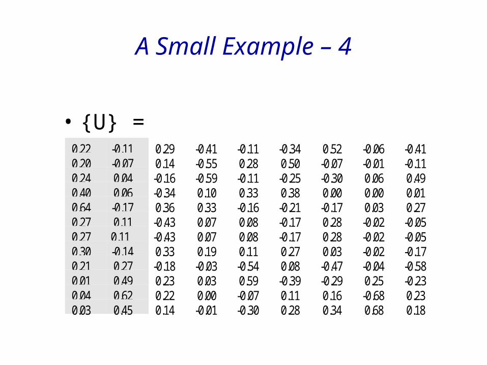
A Small Example – 4
0.22 -0.11 0.29 -0.41 -0.11 -0.34 0.52 -0.06 -0.41 0.20 -0.07 0.14 -0.55 0.28 0.50 -0.07 -0.01 -0.11 0.24 0.04 -0.16 -0.59 -0.11 -0.25 -0.30 0.06 0.49 0.40 0.06 -0.34 0.10 0.33 0.38 0.00 0.00 0.01 0.64 -0.17 0.36 0.33 -0.16 -0.21 -0.17 0.03 0.27 0.27 0.11 -0.43 0.07 0.08 -0.17 0.28 -0.02 -0.05 0.27 0.11 -0.43 0.07 0.08 -0.17 0.28 -0.02 -0.05 0.30 -0.14 0.33 0.19 0.11 0.27 0.03 -0.02 -0.17 0.21 0.27 -0.18 -0.03 -0.54 0.08 -0.47 -0.04 -0.58 0.01 0.49 0.23 0.03 0.59 -0.39 -0.29 0.25 -0.23 0.04 0.62 0.22 0.00 -0.07 0.11 0.16 -0.68 0.23 0.03 0.45 0.14 -0.01 -0.30 0.28 0.34 0.68 0.18
• {U} =

A Small Example – 5
• {S} =
3.342.54
2.351.64
1.501.31
0.850.56
0.36

A Small Example – 6
• {V} = 0.20 0.61 0.46 0.54 0.28 0.00 0.01 0.02 0.08-0.06 0.17 -0.13 -0.23 0.11 0.19 0.44 0.62 0.53 0.11 -0.50 0.21 0.57 -0.51 0.10 0.19 0.25 0.08-0.95 -0.03 0.04 0.27 0.15 0.02 0.02 0.01 -0.03 0.05 -0.21 0.38 -0.21 0.33 0.39 0.35 0.15 -0.60-0.08 -0.26 0.72 -0.37 0.03 -0.30 -0.21 0.00 0.36 0.18 -0.43 -0.24 0.26 0.67 -0.34 -0.15 0.25 0.04-0.01 0.05 0.01 -0.02 -0.06 0.45 -0.76 0.45 -0.07-0.06 0.24 0.02 -0.08 -0.26 -0.62 0.02 0.52 -0.45

A Small Example – 7
r (human.user) = .94 r (human.minors) = -.83
c1 c2 c3 c4 c5 m1 m2 m3 m4
human 0.16 0.40 0.38 0.47 0.18 -0.05 -0.12 -0.16 -0.09
interface 0.14 0.37 0.33 0.40 0.16 -0.03 -0.07 -0.10 -0.04
computer 0.15 0.51 0.36 0.41 0.24 0.02 0.06 0.09 0.12
user 0.26 0.84 0.61 0.70 0.39 0.03 0.08 0.12 0.19
system 0.45 1.23 1.05 1.27 0.56 -0.07 -0.15 -0.21 -0.05
response 0.16 0.58 0.38 0.42 0.28 0.06 0.13 0.19 0.22
time 0.16 0.58 0.38 0.42 0.28 0.06 0.13 0.19 0.22
EPS 0.22 0.55 0.51 0.63 0.24 -0.07 -0.14 -0.20 -0.11
survey 0.10 0.53 0.23 0.21 0.27 0.14 0.31 0.44 0.42
trees -0.06 0.23 -0.14 -0.27 0.14 0.24 0.55 0.77 0.66
graph -0.06 0.34 -0.15 -0.30 0.20 0.31 0.69 0.98 0.85
minors -0.04 0.25 -0.10 -0.21 0.15 0.22 0.50 0.71 0.62

LSA Titles example:Correlations between titles in raw data
c1 c2 c3 c4 c5 m1 m2 m3c2 -0.19c3 0.00 0.00c4 0.00 0.00 0.47c5 -0.33 0.58 0.00 -0.31m1 -0.17 -0.30 -0.21 -0.16 -0.17m2 -0.26 -0.45 -0.32 -0.24 -0.26 0.67m3 -0.33 -0.58 -0.41 -0.31 -0.33 0.52 0.77m4 -0.33 -0.19 -0.41 -0.31 -0.33 -0.17 0.26 0.56
0.02-0.30 0.44
Correlations in first-two dimension space
c2 0.91c3 1.00 0.91c4 1.00 0.88 1.00c5 0.85 0.99 0.85 0.81m1 -0.85 -0.56 -0.85 -0.88 -0.45m2 -0.85 -0.56 -0.85 -0.88 -0.44 1.00m3 -0.85 -0.56 -0.85 -0.88 -0.44 1.00 1.00m4 -0.81 -0.50 -0.81 -0.84 -0.37 1.00 1.00 1.00
CorrelationRaw data
0.92-0.72 1.00

Pros and Cons
• LSI puts documents together even if they don’t have common words if the docs share frequently co-occurring terms– Generally improves recall (synonymy)– Can also improve precision (polysemy)
• Disadvantages:– Slow to compute the SVD!– Statistical foundation is missing (motivation for
pLSI)
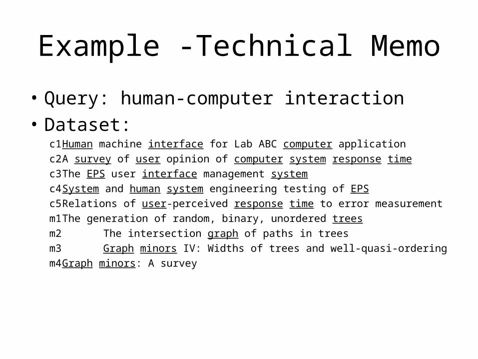
Example -Technical Memo
• Query: human-computer interaction • Dataset:
c1 Human machine interface for Lab ABC computer applicationc2 A survey of user opinion of computer system response timec3 The EPS user interface management systemc4 System and human system engineering testing of EPSc5 Relations of user-perceived response time to error measurementm1 The generation of random, binary, unordered treesm2 The intersection graph of paths in treesm3 Graph minors IV: Widths of trees and well-quasi-orderingm4 Graph minors: A survey

Example cont’% 12-term by 9-document matrix>> X=[ 1 0 0 1 0 0 0 0 0;
1 0 1 0 0 0 0 0 0;1 1 0 0 0 0 0 0 0;0 1 1 0 1 0 0 0 0;0 1 1 2 0 0 0 0 00 1 0 0 1 0 0 0 0;0 1 0 0 1 0 0 0 0;0 0 1 1 0 0 0 0 0;0 1 0 0 0 0 0 0 1;0 0 0 0 0 1 1 1 0;0 0 0 0 0 0 1 1 1;0 0 0 0 0 0 0 1 1;];

Example cont’% X=T0*S0*D0', T0 and D0 have orthonormal columns and So is diagonal% T0 is the matrix of eigenvectors of the square symmetric matrix XX'% D0 is the matrix of eigenvectors of X’X% S0 is the matrix of eigenvalues in both cases>> [T0, S0] = eig(X*X');>> T0 T0 = 0.1561 -0.2700 0.1250 -0.4067 -0.0605 -0.5227 -0.3410 -0.1063 -0.4148 0.2890 -0.1132 0.2214 0.1516 0.4921 -0.1586 -0.1089 -0.0099 0.0704 0.4959 0.2818 -0.5522 0.1350 -0.0721 0.1976 -0.3077 -0.2221 0.0336 0.4924 0.0623 0.3022 -0.2550 -0.1068 -0.5950 -0.1644 0.0432 0.2405 0.3123 -0.5400 0.2500 0.0123 -0.0004 -0.0029 0.3848 0.3317 0.0991 -0.3378 0.0571 0.4036 0.3077 0.2221 -0.0336 0.2707 0.0343 0.1658 -0.2065 -0.1590 0.3335 0.3611 -0.1673 0.6445 -0.2602 0.5134 0.5307 -0.0539 -0.0161 -0.2829 -0.1697 0.0803 0.0738 -0.4260 0.1072 0.2650 -0.0521 0.0266 -0.7807 -0.0539 -0.0161 -0.2829 -0.1697 0.0803 0.0738 -0.4260 0.1072 0.2650 -0.7716 -0.1742 -0.0578 -0.1653 -0.0190 -0.0330 0.2722 0.1148 0.1881 0.3303 -0.1413 0.3008 0.0000 0.0000 0.0000 -0.5794 -0.0363 0.4669 0.0809 -0.5372 -0.0324 -0.1776 0.2736 0.2059 0.0000 0.0000 0.0000 -0.2254 0.2546 0.2883 -0.3921 0.5942 0.0248 0.2311 0.4902 0.0127 -0.0000 -0.0000 -0.0000 0.2320 -0.6811 -0.1596 0.1149 -0.0683 0.0007 0.2231 0.6228 0.0361 0.0000 -0.0000 0.0000 0.1825 0.6784 -0.3395 0.2773 -0.3005 -0.0087 0.1411 0.4505 0.0318

Example cont’
>> [D0, S0] = eig(X'*X);>> D0 D0 =
0.0637 0.0144 -0.1773 0.0766 -0.0457 -0.9498 0.1103 -0.0559 0.1974 -0.2428 -0.0493 0.4330 0.2565 0.2063 -0.0286 -0.4973 0.1656 0.6060 -0.0241 -0.0088 0.2369 -0.7244 -0.3783 0.0416 0.2076 -0.1273 0.4629 0.0842 0.0195 -0.2648 0.3689 0.2056 0.2677 0.5699 -0.2318 0.5421 0.2624 0.0583 -0.6723 -0.0348 -0.3272 0.1500 -0.5054 0.1068 0.2795 0.6198 -0.4545 0.3408 0.3002 -0.3948 0.0151 0.0982 0.1928 0.0038 -0.0180 0.7615 0.1522 0.2122 -0.3495 0.0155 0.1930 0.4379 0.0146 -0.5199 -0.4496 -0.2491 -0.0001 -0.1498 0.0102 0.2529 0.6151 0.0241 0.4535 0.0696 -0.0380 -0.3622 0.6020 -0.0246 0.0793 0.5299 0.0820

Example cont’
>> S0=eig(X'*X)>> S0=S0.^0.5S0 = 0.3637 0.5601 0.8459 1.3064 1.5048 1.6445 2.3539 2.5417 3.3409
% We only keep the largest two singular values% and the corresponding columns from the T and D

Example cont’>> T=[0.2214 -0.1132;
0.1976 -0.0721; 0.2405 0.0432; 0.4036 0.0571;
0.6445 -0.1673; 0.2650 0.1072; 0.2650 0.1072; 0.3008 -0.1413; 0.2059 0.2736; 0.0127 0.4902; 0.0361 0.6228; 0.0318 0.4505;];>> S = [ 3.3409 0; 0 2.5417 ];>> D’ =[0.1974 0.6060 0.4629 0.5421 0.2795 0.0038 0.0146 0.0241 0.0820; -0.0559 0.1656 -0.1273 -0.2318 0.1068 0.1928 0.4379 0.6151 0.5299;]>> T*S*D’ 0.1621 0.4006 0.3790 0.4677 0.1760 -0.0527 0.1406 0.3697 0.3289 0.4004 0.1649 -0.0328 0.1525 0.5051 0.3580 0.4101 0.2363 0.0242 0.2581 0.8412 0.6057 0.6973 0.3924 0.0331 0.4488 1.2344 1.0509 1.2658 0.5564 -0.0738 0.1595 0.5816 0.3751 0.4168 0.2766 0.0559 0.1595 0.5816 0.3751 0.4168 0.2766 0.0559 0.2185 0.5495 0.5109 0.6280 0.2425 -0.0654 0.0969 0.5320 0.2299 0.2117 0.2665 0.1367 -0.0613 0.2320 -0.1390 -0.2658 0.1449 0.2404 -0.0647 0.3352 -0.1457 -0.3016 0.2028 0.3057 -0.0430 0.2540 -0.0966 -0.2078 0.1520 0.2212

Summary
• Some Issues– SVD Algorithm complexity O(n^2k^3)
• n = number of terms• k = number of dimensions in semantic space (typically
small ~50 to 350)• for stable document collection, only have to run once• dynamic document collections: might need to rerun
SVD, but can also “fold in” new documents

Summary
• Some issues– Finding optimal dimension for semantic space
• precision-recall improve as dimension is increased until hits optimal, then slowly decreases until it hits standard vector model
• run SVD once with big dimension, say k = 1000– then can test dimensions <= k
• in many tasks 150-350 works well, still room for research

Summary
• Has proved to be a valuable tool in many areas of NLP as well as IR– summarization– cross-language IR– topics segmentation– text classification– question answering– more

Summary
• Ongoing research and extensions include– Probabilistic LSA (Hofmann)– Iterative Scaling (Ando and Lee)– Psychology
• model of semantic knowledge representation• model of semantic word learning

Probabilistic Topic Models• A probabilistic version of LSA: no spatial
constraints.
• Originated in domain of statistics & machine learning– (e.g., Hoffman, 2001; Blei, Ng, Jordan, 2003)
• Extracts topics from large collections of text

DATACorpus of text:
Word counts for each document
Topic Model
Find parameters that “reconstruct” data
Model is Generative

Probabilistic Topic Models
• Each document is a probability distribution over topics (distribution over topics = gist)
• Each topic is a probability distribution over words

Document generation as a probabilistic process
TOPICS MIXTURETOPICS MIXTURE
TOPIC TOPIC TOPICTOPIC
WORDWORD WORDWORD
......
......
1. for each document, choosea mixture of topics
2. For every word slot, sample a topic [1..T] from the mixture
3. sample a word from the topic

loan
TOPIC 1
money
loan
bank
moneyba
nk
river
TOPIC 2
river
river
stream
bank
bank
stream
bank
loan
DOCUMENT 2: river2 stream2 bank2 stream2 bank2 money1 loan1
river2 stream2 loan1 bank2 river2 bank2 bank1 stream2 river2 loan1
bank2 stream2 bank2 money1 loan1 river2 stream2 bank2 stream2 bank2 money1 river2 stream2 loan1 bank2 river2 bank2 money1 bank1 stream2 river2 bank2 stream2 bank2 money1
DOCUMENT 1: money1 bank1 bank1 loan1 river2 stream2 bank1
money1 river2 bank1 money1 bank1 loan1 money1 stream2 bank1
money1 bank1 bank1 loan1 river2 stream2 bank1 money1 river2 bank1
money1 bank1 loan1 bank1 money1 stream2
.3
.8
.2
Example
Mixture components
Mixture weights
Bayesian approach: use priors Mixture weights ~ Dirichlet( ) Mixture components ~ Dirichlet( )
.7

DOCUMENT 2: river? stream? bank? stream? bank? money? loan?
river? stream? loan? bank? river? bank? bank? stream? river? loan?
bank? stream? bank? money? loan? river? stream? bank? stream? bank? money? river? stream? loan? bank? river? bank? money? bank? stream? river? bank? stream? bank? money?
DOCUMENT 1: money? bank? bank? loan? river? stream? bank?
money? river? bank? money? bank? loan? money? stream? bank?
money? bank? bank? loan? river? stream? bank? money? river? bank?
money? bank? loan? bank? money? stream?
Inverting (“fitting”) the model
Mixture components
Mixture weights
TOPIC 1
TOPIC 2
?
?
?

Application to corpus data
• TASA corpus: text from first grade to college– representative sample of text
• 26,000+ word types (stop words removed)• 37,000+ documents• 6,000,000+ word tokens

Example: topics from an educational corpus (TASA)
PRINTINGPAPERPRINT
PRINTEDTYPE
PROCESSINK
PRESSIMAGE
PRINTERPRINTS
PRINTERSCOPY
COPIESFORM
OFFSETGRAPHICSURFACE
PRODUCEDCHARACTERS
PLAYPLAYSSTAGE
AUDIENCETHEATERACTORSDRAMA
SHAKESPEAREACTOR
THEATREPLAYWRIGHT
PERFORMANCEDRAMATICCOSTUMES
COMEDYTRAGEDY
CHARACTERSSCENESOPERA
PERFORMED
TEAMGAME
BASKETBALLPLAYERSPLAYER
PLAYPLAYINGSOCCERPLAYED
BALLTEAMSBASKET
FOOTBALLSCORECOURTGAMES
TRYCOACH
GYMSHOT
JUDGETRIAL
COURTCASEJURY
ACCUSEDGUILTY
DEFENDANTJUSTICE
EVIDENCEWITNESSES
CRIMELAWYERWITNESS
ATTORNEYHEARING
INNOCENTDEFENSECHARGE
CRIMINAL
HYPOTHESISEXPERIMENTSCIENTIFIC
OBSERVATIONSSCIENTISTS
EXPERIMENTSSCIENTIST
EXPERIMENTALTEST
METHODHYPOTHESES
TESTEDEVIDENCE
BASEDOBSERVATION
SCIENCEFACTSDATA
RESULTSEXPLANATION
STUDYTEST
STUDYINGHOMEWORK
NEEDCLASSMATHTRY
TEACHERWRITEPLAN
ARITHMETICASSIGNMENT
PLACESTUDIED
CAREFULLYDECIDE
IMPORTANTNOTEBOOK
REVIEW
• 37K docs, 26K words• 1700 topics, e.g.:

Polysemy
PRINTINGPAPERPRINT
PRINTEDTYPE
PROCESSINK
PRESSIMAGE
PRINTERPRINTS
PRINTERSCOPY
COPIESFORM
OFFSETGRAPHICSURFACE
PRODUCEDCHARACTERS
PLAYPLAYSSTAGE
AUDIENCETHEATERACTORSDRAMA
SHAKESPEAREACTOR
THEATREPLAYWRIGHT
PERFORMANCEDRAMATICCOSTUMES
COMEDYTRAGEDY
CHARACTERSSCENESOPERA
PERFORMED
TEAMGAME
BASKETBALLPLAYERSPLAYERPLAY
PLAYINGSOCCERPLAYED
BALLTEAMSBASKET
FOOTBALLSCORECOURTGAMES
TRYCOACH
GYMSHOT
JUDGETRIAL
COURTCASEJURY
ACCUSEDGUILTY
DEFENDANTJUSTICE
EVIDENCEWITNESSES
CRIMELAWYERWITNESS
ATTORNEYHEARING
INNOCENTDEFENSECHARGE
CRIMINAL
HYPOTHESISEXPERIMENTSCIENTIFIC
OBSERVATIONSSCIENTISTS
EXPERIMENTSSCIENTIST
EXPERIMENTALTEST
METHODHYPOTHESES
TESTEDEVIDENCE
BASEDOBSERVATION
SCIENCEFACTSDATA
RESULTSEXPLANATION
STUDYTEST
STUDYINGHOMEWORK
NEEDCLASSMATHTRY
TEACHERWRITEPLAN
ARITHMETICASSIGNMENT
PLACESTUDIED
CAREFULLYDECIDE
IMPORTANTNOTEBOOK
REVIEW

Three documents with the word “play”(numbers & colors topic assignments)
A Play082 is written082 to be performed082 on a stage082 before a live093 audience082 or before motion270 picture004 or television004 cameras004 ( for later054 viewing004 by large202 audiences082). A Play082 is written082 because playwrights082 have something ... He was listening077 to music077 coming009 from a passing043 riverboat. The music077 had already captured006 his heart157 as well as his ear119. It was jazz077. Bix beiderbecke had already had music077 lessons077. He wanted268 to play077 the cornet. And he wanted268 to play077 jazz077... J im296 plays166 the game166. J im296 likes081 the game166 for one. The game166 book254 helps081 jim296. Don180 comes040 into the house038. Don180 and jim296 read254 the game166 book254. The boys020 see a game166 for two. The two boys020 play166 the game166....

No Problem of Triangle Inequality
SOCCER
MAGNETICFIELD
TOPIC 1 TOPIC 2
Topic structure easily explains violations of triangle inequality

Applications

Enron email data 500,000 emails500,000 emails
5000 authors5000 authors
1999-20021999-2002

Enron topics
2000 2001 2002 2003
PERSON1
PERSON2
TEXANSWIN
FOOTBALLFANTASY
SPORTSLINEPLAYTEAMGAME
SPORTSGAMES
GODLIFEMAN
PEOPLECHRISTFAITHLORDJESUS
SPIRITUALVISIT
ENVIRONMENTALAIR
MTBEEMISSIONS
CLEANEPA
PENDINGSAFETYWATER
GASOLINE
FERCMARKET
ISOCOMMISSION
ORDERFILING
COMMENTSPRICE
CALIFORNIAFILED
POWERCALIFORNIAELECTRICITY
UTILITIESPRICESMARKET
PRICEUTILITY
CUSTOMERSELECTRIC
STATEPLAN
CALIFORNIADAVISRATE
BANKRUPTCYSOCALPOWERBONDSMOU
TIMELINEMay 22, 2000Start of California
energy crisis

Probabilistic Latent Semantic Analysis
• Automated Document Indexing and Information retrieval
Identification of Latent Classes using an Expectation Maximization (EM) Algorithm
Shown to solve Polysemy
Java could mean “coffee” and also the “PL Java” Cricket is a “game” and also an “insect”
Synonymy “computer”, “pc”, “desktop” all could mean the same
Has a better statistical foundation than LSA

PLSA
• Aspect Model• Tempered EM• Experiment Results

PLSA – Aspect Model
• Aspect Model– Document is a mixture of underlying (latent) K
aspects – Each aspect is represented by a distribution of
words p(w|z)
• Model fitting with Tempered EM

Aspect Model
• Generative Model– Select a doc with probability P(d)– Pick a latent class z with probability P(z|d)– Generate a word w with probability p(w|z)
d z wP(d) P(z|d) P(w|z)
Latent Variable model for general co-occurrence data Associate each observation (w,d) with a class variable z Є
Z{z_1,…,z_K}

Aspect Model
• To get the joint probability model

• Using Bayes’ rule

Advantages of this model over Documents Clustering
• Documents are not related to a single cluster (i.e. aspect )– For each z, P(z|d) defines a specific mixture of
factors– This offers more flexibility, and produces effective
modeling
Now, we have to compute P(z), P(z|d), P(w|z). We are given just documents(d) and words(w).

Model fitting with Tempered EM
• We have the equation for log-likelihood function from the aspect model, and we need to maximize it.
• Expectation Maximization ( EM) is used for this purpose– To avoid overfitting, tempered EM is proposed

Expectation Maximization (EM)
Involves three entities:1)Observed data X
– In our case, X is both d(ocuments) and w(ords)
2) Latent data Y- In our case, Y is the latent topics z
3) Parameters θ- In our case, θ contains values for P(z),
P(w|z), and P(d|z), for all choices of z, w, and d.

EM Intuition
• EM is used to maximize a (log) likelihood function when some of the data is latent.
• Both Y and θ are unknowns, X is known.• Instead of searching over just θ to improve LL,
– EM searches over θ and Y– It starts with an initial guess for one of them (let’s say Y)– Then it estimates θ given the current estimate of Y– Then it estimates Y given the current estimate of θ– …
• EM is guaranteed to converge to a local optimum of the LL

EM Steps
• E-Step– Expectation step where the expected (posterior)
distribution of the latent variables is calculated– Uses the current estimate of the parameters
• M-Step– Maximization step: Find the parameters that
maximizes the likelihood function – Uses the current estimate of the latent variables

E Step
Compute a posterior distribution for the latent topic variables, using current parameters.
(after some algebra)

M Step
Compute maximum-likelihood parameter estimates.
All these equations use P(z|d,w), which was calculated in the E-Step.

Over fitting
• Trade off between Predictive performance on the training data and Unseen new data
• Must prevent the model to over fit the training data
• Propose a change to the E-Step
• Reduce the effect of fitting as we do more steps

TEM (Tempered EM)
• Introduce control parameter β
• β starts from the value of 1, and decreases

Simulated Annealing
• Alternate healing and cooling of materials to make them attain a minimum internal energy state – reduce defects
• This process is similar to Simulated Annealing : β acts a temperature variable
• As the value of β decreases, the effect of re-estimations don’t affect the expectation calculations

Choosing β
• How to choose a proper β?• It defines
– Underfit Vs Overfit • Simple solution using held-out data (part of
training data)– Using the training data for β starting from 1– Test the model with held-out data– If improvement, continue with the same β– If no improvement, β <- nβ where n<1

Perplexity Comparison(1/4)
• Perplexity – Log-averaged inverse probability on unseen data• High probability will give lower perplexity, thus good
predictions
• MED data

Topic Decomposition(2/4)
• Abstracts of 1568 documents• Clustering 128 latent classes
• Shows word stems for the same word “power” as p(w|z)
Power1 – AstronomyPower2 - Electricals

Polysemy(3/4)
• “Segment” occurring in two different contexts are identified (image, sound)

Information Retrieval(4/4)
• MED – 1033 docs• CRAN – 1400 docs• CACM – 3204 docs• CISI – 1460 docs
• Reporting only the best results with K varying from 32, 48, 64, 80, 128
• PLSI* model takes the average across all models at different K values

Information Retrieval (4/4)
• Cosine Similarity is the baseline• In LSI, query vector(q) is multiplied to get the
reduced space vector• In PLSI, p(z|d) and p(z|q). In EM iterations, only P(z|
q) is adapted

Precision-Recall results(4/4)

Comparing PLSA and LSA• LSA and PLSA perform dimensionality reduction
– In LSA, by keeping only K singular values– In PLSA, by having K aspects
• Comparison to SVD– U Matrix related to P(d|z) (doc to aspect)– V Matrix related to P(z|w) (aspect to term)– E Matrix related to P(z) (aspect strength)
• The main difference is the way the approximation is done– PLSA generates a model (aspect model) and maximizes its predictive
power– Selecting the proper value of K is heuristic in LSA– Model selection in statistics can determine optimal K in PLSA

Latent Dirichlet Allocation

“Bag of Words” Models
• Let’s assume that all the words within a document are exchangeable.

Mixture of Unigrams
Mixture of Unigrams Model (this is just Naïve Bayes)
For each of M documents, Choose a topic z. Choose N words by drawing each one independently from a multinomial
conditioned on z.
In the Mixture of Unigrams model, we can only have one topic per document!
Zi
w4iw3iw2iwi1

The pLSI Model
Probabilistic Latent Semantic Indexing (pLSI) Model
For each word of document d in the training set,
Choose a topic z according to a multinomial conditioned on the index d.
Generate the word by drawing from a multinomial conditioned on z.
In pLSI, documents can have multiple topics.
d
zd4zd3zd2zd1
wd4wd3wd2wd1

Motivations for LDA• In pLSI, the observed variable d is an index into some training set. There is
no natural way for the model to handle previously unseen documents.• The number of parameters for pLSI grows linearly with M (the number of
documents in the training set).• We would like to be Bayesian about our topic mixture proportions.

Dirichlet Distributions• In the LDA model, we would like to say that the topic mixture proportions
for each document are drawn from some distribution.• So, we want to put a distribution on multinomials. That is, k-tuples of
non-negative numbers that sum to one.• The space of all of these multinomials has a nice geometric interpretation
as a (k-1)-simplex, which is just a generalization of a triangle to (k-1) dimensions.
• Criteria for selecting our prior:– It needs to be defined for a (k-1)-simplex.– Algebraically speaking, we would like it to play nice with the multinomial
distribution.

Dirichlet Examples

Dirichlet Distributions
• Useful Facts:– This distribution is defined over a (k-1)-simplex. That is, it takes k non-
negative arguments which sum to one. Consequently it is a natural distribution to use over multinomial distributions.
– In fact, the Dirichlet distribution is the conjugate prior to the multinomial distribution. (This means that if our likelihood is multinomial with a Dirichlet prior, then the posterior is also Dirichlet!)
– The Dirichlet parameter i can be thought of as a prior count of the ith class.

The LDA Model
z4z3z2z1
w4w3w2w1
z4z3z2z1
w4w3w2w1
z4z3z2z1
w4w3w2w1
• For each document,• Choose ~Dirichlet()• For each of the N words wn:
– Choose a topic zn» Multinomial()
– Choose a word wn from p(wn|zn,), a multinomial probability conditioned on the topic zn.

The LDA Model
For each document,• Choose » Dirichlet()• For each of the N words wn:
– Choose a topic zn» Multinomial()
– Choose a word wn from p(wn|zn,), a multinomial probability conditioned on the topic zn.

Inference
•The inference problem in LDA is to compute the posterior of the hidden variables given a document and corpus parameters and . That is, compute p(,z|w,,).
•Unfortunately, exact inference is intractable, so we turn to alternatives…

Variational Inference
•In variational inference, we consider a simplified graphical model with variational parameters , and minimize the KL Divergence between the variational and posterior distributions.

Parameter Estimation• Given a corpus of documents, we would like to find the parameters and which
maximize the likelihood of the observed data.• Strategy (Variational EM):
– Lower bound log p(w|,) by a function L(,;,)– Repeat until convergence:
• Maximize L(,;,) with respect to the variational parameters ,.• Maximize the bound with respect to parameters and .

Some Results• Given a topic, LDA can return the most probable words.• For the following results, LDA was trained on 10,000 text articles posted to 20
online newsgroups with 40 iterations of EM. The number of topics was set to 50.

Some Results
Political Team Space Drive God
Party Game NASA Windows Jesus
Business Play Research Card His
Convention Year Center DOS Bible
Institute Games Earth SCSI Christian
Committee Win Health Disk Christ
States Hockey Medical System Him
Rights Season Gov Memory Christians
“politics” “sports” “space” “computers” “christianity”

Extensions/Applications
• Multimodal Dirichlet Priors• Correlated Topic Models• Hierarchical Dirichlet Processes• Abstract Tagging in Scientific Journals• Object Detection/Recognition

Visual Words• Idea: Given a collection of images,
– Think of each image as a document.– Think of feature patches of each image as words.– Apply the LDA model to extract topics.
(J. Sivic, B. C. Russell, A. A. Efros, A. Zisserman, W. T. Freeman. Discovering object categories in image collections. MIT AI Lab Memo AIM-2005-005, February, 2005. )

Visual Words
Examples of ‘visual words’

Visual Words

References
Latent Dirichlet allocation. D. Blei, A. Ng, and M. Jordan. Journal of Machine Learning Research, 3:993-1022, January 2003.
Finding Scientific Topics. Griffiths, T., & Steyvers, M. (2004). Proceedings of the National Academy of Sciences, 101 (suppl. 1), 5228-5235.
Hierarchical topic models and the nested Chinese restaurant process. D. Blei, T. Griffiths, M. Jordan, and J. Tenenbaum In S. Thrun, L. Saul, and B. Scholkopf, editors, Advances in Neural Information Processing Systems (NIPS) 16, Cambridge, MA, 2004. MIT Press.
Discovering object categories in image collections. J. Sivic, B. C. Russell, A. A. Efros, A. Zisserman, W. T. Freeman. MIT AI Lab Memo AIM-2005-005, February, 2005.

92
Latent Dirichlet allocation (cont.)• The joint distribution of a topic θ, and a set of N topic
z, and a set of N words w:
• Marginal distribution of a document:
• Probability of a corpus:
dzwpzpppN
n znnn
n
w
1
,|||,|
N
nnnn zwpzppp
1
,|||,| wz,,
M
dd
N
n zdndndnd dzwpzppDp
d
dn1 1
,|||,|

93
Latent Dirichlet allocation (cont.)• There are three levels to LDA representation
– α, β are corpus-level parameters– θd are document-level variables– zdn, wdn are word-level variables
corpusdocument

94
Latent Dirichlet allocation (cont.)• LDA and exchangeability
– A finite set of random variables {z1,…,zN} is said exchangeable if the joint distribution is invariant to permutation (π is a permutation)
– A infinite sequence of random variables is infinitely exchangeable if every finite subsequence is exchangeable
– De Finetti’s representation theorem states that the joint distribution of an infinitely exchangeable sequence of random variables is as if a random parameter were drawn from some distribution and then the random variables in question were independent and identically distributed, conditioned on that parameter
– http://en.wikipedia.org/wiki/De_Finetti's_theorem
NN zzpzzp ,...,,..., 11

95
Latent Dirichlet allocation (cont.)
• In LDA, we assume that words are generated by topics (by fixed conditional distributions) and that those topics are infinitely exchangeable within a document
dzwpzpppN
nnnn zw,
1
||

96
Latent Dirichlet allocation (cont.)• A continuous mixture of unigrams
– By marginalizing over the hidden topic variable z, we can understand LDA as a two-level model
• Generative process for a document w– 1. choose θ~ Dir(α)– 2. For each of the N word wn
(a) Choose a word wn from p(wn|θ, β)– Marginal distribution of a document
z
zpzwpwp |,|,|
dwppwpN
nn
1
,||,|
97
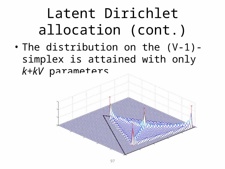
Latent Dirichlet allocation (cont.)
• The distribution on the (V-1)-simplex is attained with only k+kV parameters.

98
Relationship with other latent variable models
• Unigram model
• Mixture of unigrams– Each document is generated by first choosing a topic z and
then generating N words independently form conditional multinomial
– k-1 parameters
N
nnwpwp
1
z
N
nn zwpzpwp
1
|

99
Relationship with other latent variable models (cont.)
• Probabilistic latent semantic indexing– Attempt to relax the simplifying assumption made in the
mixture of unigrams models– In a sense, it does capture the possibility that a document
may contain multiple topics– kv+kM parameters and linear growth in M
z
nn dzpzwpdpwdp ||,

100
Relationship with other latent variable models (cont.)
• Problem of PLSI– There is no natural way to use it to assign probability to a
previously unseen document– The linear growth in parameters suggests that the model is
prone to overfitting and empirically, overfitting is indeed a serious problem
• LDA overcomes both of these problems by treating the topic mixture weights as a k-parameter hidden random variable
• The k+kV parameters in a k-topic LDA model do not grow with the size of the training corpus.

101
Relationship with other latent variable models (cont.)
• The unigram model find a single point on the word simplex and posits that all word in the corpus come from the corresponding distribution.
• The mixture of unigram models posits that for each documents, one of the k points on the word simplex is chosen randomly and all the words of the document are drawn from the distribution
• The pLSI model posits that each word of a training documents comes from a randomly chosen topic. The topics are themselves drawn from a document-specific distribution over topics.
• LDA posits that each word of both the observed and unseen documents is generated by a randomly chosen topic which is drawn from a distribution with a randomly chosen parameter

102
Inference and parameter estimation
• The key inferential problem is that of computing the posteriori distribution of the hidden variable given a document
,|
,|,,,,|,
w
wzwz
p
pp
dp
N
n
k
i
V
j
wiji
k
iik
i i
k
i i jni w
1 1 11
1
1
1,|
Unfortunately, this distribution is intractable to compute in general.A function which is intractable due to the coupling between θ and β in the summation over latent topics

103
Inference and parameter estimation (cont.)
• The basic idea of convexity-based variational inference is to make use of Jensen’s inequality to obtain an adjustable lower bound on the log likelihood.
• Essentially, one considers a family of lower bounds, indexed by a set of variational parameters.
• A simple way to obtain a tractable family of lower bound is to consider simple modifications of the original graph model in which some of the edges and nodes are removed.

104
Inference and parameter estimation (cont.)
• Drop some edges and the w nodes
N
nnnzqqq
1
||,|, z
,|
,|,,,,|,
w
wzwz
p
pp

105
Inference and parameter estimation (cont.)
• Variational distribution:– Lower bound on Log-likelihood
– KL between variational posterior and true posterior
,|,,|,,log,|,
,|,,log,|,
,|,
,|,,,|,log,|,,log,|log
zwzz
wzz
z
wzz wzw
z
z
qEpEdq
pq
dq
pqdpp
z
,log,,,,|,
,
,,,log,|,,|,log,|,
,,log,|,,|,log,|,
,,||,|,
,pE,pEqE
d,p
,pqdqq
d,|pqdqq
,|pqD
qqq wwzz
w
wzzzz
wzzzz
wzz
zz
zz

106
Inference and parameter estimation (cont.)
• Finding a tight lower bound on the log likelihood
• Maximizing the lower bound with respect to γand φ is equivalent to minimizing the KL divergence between the variational posterior probability and the true posterior probability
,,||,|,
,|,log,|,,log,|log
,|pqD
qEpEp qq
wzz
zwzw
,,||,|,minarg,,
** ,|pqD wzz

107
Inference and parameter estimation (cont.)
• Expand the lower bound:
|log
|log
,|log
|log
|log
,|,log,|,,log,;,
z
zw
z
zwz
pE
pE
pE
pE
pE
qEpEL
q
q
q
q
q

108
Inference and parameter estimation (cont.)
• Then
N
n
k
inini
k
i
k
j jiii
k
i
k
j j
N
n
k
iij
jnni
N
n
k
i
k
j jini
k
i
k
j jiii
k
i
k
j j
w
L
1 1
11
11
1 1
1 11
11
11
log
1loglog
log
1loglog
,;,

109
Inference and parameter estimation (cont.)
• We can get variational parameters by adding Lagrange multipliers and setting this derivative to zero:
N
n niii
k
j jiivni
1
1exp

110
Inference and parameter estimation (cont.)
• Parameter estimation– Maximize log likelihood of the data:
– Variational inference provide us with a tractable lower bound on the log likelihood, a bound which we can maximize with respect α and β
• Variational EM procedure– 1. (E-step) For each document, find the optimizing values
of the variational parameters {γ, φ}– 2. (M-step) Maximize the resulting lower bound on the log
likelihood with respect to the model parameters α and β
M
ddp
1
,|log, w

111
Inference and parameter estimation (cont.)
• Smoothed LDA model:

112
Discussion• LDA is a flexible generative probabilistic model
for collection of discrete data.
• Exact inference is intractable for LDA, but any or a large suite of approximate inference algorithms for inference and parameter estimation can be used with the LDA framework.
• LDA is a simple model and is readily extended to continuous data or other non-multinomial data.

Relation to Text Classification and Information Retrieval

LSI for IR
• Compute cosine similarity for document and query vectors in semantic space– Helps combat synonymy– Helps combat polysemy in documents, but not
necessarily in queries (which were not part of the SVD computation)

pLSA/LDA for IR
• Several options– Compute cosine similarity between topic vectors
for documents– Use language model-based IR techniques
• potentially very helpful for synonymy and polysemy

LDA/pLSA for Text Classification
• Topic models are easy to incorporate into text classification:1. Train a topic model using a big corpus2. Decode the topic model (find best topic/cluster
for each word) on a training set3. Train classifier using the topic/cluster as a
feature4. On a test document, first decode the topic
model, then make a prediction with the classifier

Why use a topic model for classification?
• Topic models help handle polysemy and synonymy– The count for a topic in a document can be much
more informative than the count of individual words belonging to that topic.
• Topic models help combat data sparsity– You can control the number of topics– At a reasonable choice for this number, you’ll observe
the topics many times in training data(unlike individual words, which may be very sparse)

LSA for Text Classification
• Trickier to do– One option is to use the reduced-dimension
document vectors for training– At test time, what to do?
• Can recalculate the SVD (expensive)– Another option is to combine the reduced-
dimension term vectors for a given document to produce a vector for the document
– This is repeatable at test time (at least for words that were seen during training)