luis g. bergh - codelco · monitoreo y diagnostico de la operaciÓ de flotacion usando tecnicas de...
TRANSCRIPT

MONITOREO Y DIAGNOSTICO DE LA MONITOREO Y DIAGNOSTICO DE LA OPERACIOPERACIÓÓN DE PROCESOS DE N DE PROCESOS DE
FLOTACION USANDO TECNICAS DE FLOTACION USANDO TECNICAS DE PROYECCIONPROYECCION
Luis G. BerghLuis G. BerghCentro de AutomatizaciCentro de Automatizacióón y Supervisin y Supervisióón para la Industria Minera n para la Industria Minera
(CASIM)(CASIM)Universidad TUniversidad Téécnica Federico Santa Marcnica Federico Santa Marííaa
ValparaValparaííso, Chileso, Chile

ContenidoContenido
•• CaracterCaracteríísticas del problemasticas del problema•• Como extraer informaciComo extraer informacióón desde miles de datos n desde miles de datos (T(Téécnicas de estadcnicas de estadíística multivariable, PLS y PCA)stica multivariable, PLS y PCA)•• Aplicaciones en toma de decisiones:Aplicaciones en toma de decisiones:
•• Monitoreo en linea de columnas de flotaciMonitoreo en linea de columnas de flotacióónn•• Monitoreo en linea de circuitos de flotaciMonitoreo en linea de circuitos de flotacióónn
•• ConclusionesConclusiones
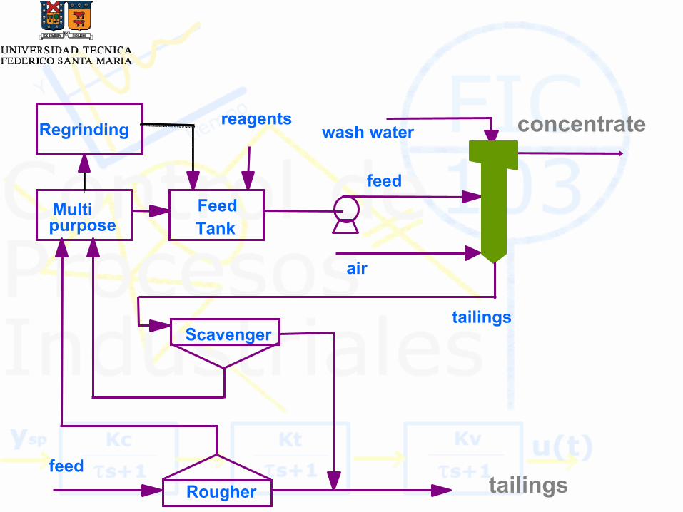
FeedTank
Multipurpose
Regrinding
tailings
Scavenger
Rougher
wash water
air
feed
tailings
feed
concentratereagents

LIC
Concentrate andConcentrate and
Column design parameters:Diameter, hight, geometry, spargers,
Water distributors, lip size,…
Tailings gradesTailings grades
Depend on many Depend on many input variablesinput variables
Wash water flowrate
Air flowrate
FI
FI
Feed characteristics:Flow, mineralogical species, density, solid percentage, particle size distribution, grades, chemical reagents…
Froth depth
Gas holdup

25
27
29
31
33
0 200 400 600
Sample number
Con
c. g
rade
60
65
70
75
80
85
90
Rec
over
y %
Concentrate grade Recovery
¿Quién es el culpable?

LIC
Concentrate andConcentrate and
Column design parameters:Diameter, hight, geometry, spargers,
Water distributors, lip size,…
Tailings gradesTailings grades
Depend on many Depend on many input variablesinput variables
Wash water flowrate
Air flowrate
FI
FI
Feed characteristics:Flow, mineralogical species, density, solid percentage, particle size distribution, grades, chemical reagents…
Froth depth
Gas holdup

Si existen N variables de entrada tenemos un problema de dimensión N que resolver (muy complejo) y si las variables están correlacionadas entre si se agrega un problema de estimación de parámetros del modelo
¿Cómo extraer información relevante de un conjunto de datos?


Un perro es un objeto real que tiene un volumen (tres dimensiones), pero podemos PROYECTAR una imagen en una dimensión menor (dos).
Al observar la imagen de la realidad la identificamos y la entendemos como lo que es.
¿Un proceso puede tener dimensión N, pero podemos proyectar su imagen en menos dimensiones?

Geometric interpretation
Variable 1
Variable 2
Variable 3

Geometric interpretation
Variable 1
Variable 2
Variable 3
V =f1(x,y,z)W=f2(x,y,z)v

Si existen N variables de entrada tenemos un problema de dimensión N que resolver (muy complejo) y si las variables están correlacionadas entre si se agrega un problema de estimación de parámetros del modelo
Si algunas variables de entrada estuvieran CORRELACIONADAS entre si, tenemos un problema de estimación, pero una oportunidad de reducir la dimensión del problema a resolver (menos complejo)
PROYECCION

Geometric interpretation
Variable 1
Variable 2
Variable 3
1st PC
2nd PC

Si existen N variables de entrada tenemos un problema de dimensión N que resolver (muy complejo) y si las variables están correlacionadas entre si se agrega un problema de estimación de parámetros del modelo
Si algunas variables de entrada estuvieran CORRELACIONADAS entre si, tenemos un problema de estimación, pero una oportunidad de reducir la dimensión del problema a resolver (menos complejo) PROYECCION
Si existiera un conjunto menor de variables auxiliares, que siendo una función lineal de las variables de entrada, fueran INDEPENDIENTES entre si, entonces tenemos un problema de dimensión menor que resolver y una condición óptima de estimación de parámetros de un modelo
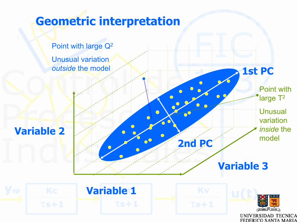
Geometric interpretation
Variable 1
Variable 2
Variable 3
1st PC
2nd PC
Point with large Q2
Unusual variation outside the model
Point with large T2
Unusual variation inside the model

On-line tests based on the following criteria:
•Normal operation if the new set of data satisfies the Q and T2 test.
•Abnormal operation if only the T2 test is failed.
•Measurement problem or PCA model representation problem if only T2 test is satisfied.
•If both test failed then either the model is no longer appropriate or a measurement problem occurred.
•Which combination of input variables may explain this?

EIC1
LIC1
TK-1
FIC1
FIC2
Feed pump
BIC-1
GE-9030PLC
-
PC networkIntouch
Air
Concentrate

Flotation Process
Design parameters:Diameter, height, geometry…
Feed characteristics:species, density, solid percentage, particle size, grades, kinetic constants, chemical reagents…
Concentrate gradeTailings gradeRecoveryBias rateGas hold up
froth depthair flow ratewater flow ratefeed flow rate

1. Collecting a set of data under different operating conditions
2. Select a subset that satisfies a so called normal condition
(concentrate grade inside a band and a minimum recovery)
3. Select the number of Principal Components that explains a
given variance (for example using PLS_toolbox with
Matlab)
4. Build a PCA model and obtain the Q and T2 test limits
5. Implement the test on-line
6. Interpret the results.

N° Variable Tag1 Froth depth z2 Gas hold up E3 Dp/cell low LL4 Dp/cell high LH5 Pressure to air control valve PA6 Pressure to Tailings control valve PT7 Bias superficial velocity Jb8 Air superficial velocity Jg9 Tailings superficial velocity Jt10 Feed superficial velocity Jf11 Wash water superficial velocity Jw12 Cu recovery R13 Concentrate Cu grade CCG14 Feed particle size d80 D15 Feed Cu grade FCG16 Feed solid percentage S

-0,5
0
0,5
1
1 2 3 4 5 6
Principal components
Con
tribu
tion
%
All variables were included in the model. The first components showed the contribution of groups of correlated variables, while the last ones mostly represented the bias and the feed characteristics. For monitoring: T2 = 12.6, Q = 3.81.

0
2
4
6
8
0 200 400 600Sample number
Q re
sidu
als
0
10
20
30
0 200 400 600Sample number
Hot
ellin
g
25
27
29
31
33
0 200 400 600Sample number
Con
c. g
rade
60657075808590
Rec
over
y %
Concentrate grade Recovery

0
10
20
30
z E PL PH PA PT Jb Jf Jg Jt Jw R CCG D FCG S
% re
sidu
al T
i
0
50
100
150
0 200 400 600Sample number
Frot
h de
pth
[cm
]

0
2
4
6
8
0 200 400 600Sample number
Q re
sidu
als
0
10
20
30
0 200 400 600Sample number
Hot
ellin
g
25
27
29
31
33
0 200 400 600Sample number
Con
c. g
rade
60657075808590
Rec
over
y %
Concentrate grade Recovery

0
5
10
15
-15 -5 5 15Error %
Q re
sidu
als
Failure detection on virtual concentrate grade

On stream analysers
Particle size
Pulp level
Froth image
Density
0.7 MMDTPY of concentrate
1 line 2-3-3-3-3 array


Espuma Dura. Espuma Mojada. Espuma Seca.

Froth characteristics: correlation with concentrate grade and recovery
• bubble diameter distribution, • the percentage of different classes of bubble diameter, • the mineral charge on the bubble (as the proportional area of the bubble covered by mineral), • the RGB color, HSV color, Lab color, • tint, brightness, luminescence, • dispersion, collapse ratio, texture, image stability, • x velocity, y velocity, velocity module.

Froth characteristics: correlation with concentrate grade
and recovery
• Past research with no concrete results
• Today more than 1000 cameras installed in Chile
• Main benefit has been to associate velocity and pulp level
control set point
¿Qué falta?

Hypothesis:
Froth images are from top of froth
In the froth there is a distribution of properties (grade, solid percentage, particle size,…) that is influenced by operating variables (flow rates, froth depth, reactive dossages, feed characteristics, …)
Correlation between ALL VARIABLES

Operating Variables
Primary collector flow rate Rougher feed copper gradeSecondary collector flow rate (cell 1) Concentrate copper gradeSecondary collector flow rate (cell 6) Tailings copper gradeCell 1 frother flow rate Copper rougher recoveryCell 5 frother flow rate Rougher feed iron gradeFroth depth at cell 2 Mineral densityFroth depth at cell 5 Rougher feed solid tonnageFroth depth at cell 8 Total water flow rateFroth depth at cell 11 Rougher feed solid percentage
Froth depth at cell 14

Escala entrega el valor de R para cada par de variablesEscala entrega el valor de R para cada par de variables

Variable PC 1 PC 2 PC 3 PC 4 PC 5 PC 6 PC 7Brillantez Medida en la Celda 1 0,185 -0,007 -0,070 -0,068 -0,078 0,110 0,263Color Azul Medida en la Celda 1 0,105 0,126 -0,394 -0,147 0,050 -0,021 -0,056Color Rojo Medida en la Celda 1 0,139 0,016 -0,334 -0,139 0,149 0,108 -0,139Color Verde Medida en la Celda 1 0,142 0,065 -0,332 -0,119 0,136 0,025 -0,122Perfil HSV Medida en la Celda 1 -0,111 -0,134 0,123 -0,046 -0,215 0,452 -0,104Pureza (HSV) Medida en la Celda 1 -0,142 0,153 -0,099 -0,076 -0,330 -0,213 0,233Tinte (HSV) Medida en la Celda 1 -0,114 0,256 -0,124 -0,004 -0,209 -0,230 0,271Value (HSV) Medida en la Celda 1 0,107 0,104 -0,397 -0,157 0,055 -0,009 -0,060Luminiscencia (LAB Color) Medida en la Celda 1 0,141 0,065 -0,330 -0,104 0,171 0,001 -0,118Parámetro AX (LAB Color) Medida en la Celda 1 -0,141 -0,096 -0,144 -0,166 -0,185 0,304 0,083Parámetro BX (LAB Color) Medida en la Celda 1 0,132 -0,217 0,141 0,060 0,298 0,192 -0,221Carga de Burbujas Medida en la Celda 1 -0,167 -0,134 0,045 0,022 0,142 -0,177 -0,080Textura de Burbujas Medida en la Celda 1 0,203 -0,010 0,051 -0,010 -0,121 -0,042 -0,041Módulo de Velocidad de Espuma Medida en la Celda 1 0,170 0,175 0,119 0,092 -0,037 -0,079 -0,227Velocidad de Espuma en Eje X Medida en la Celda 1 -0,135 0,034 0,044 -0,220 0,187 0,164 0,338Velocidad de Espuma en Eje Y Medida en la Celda 1 -0,169 -0,180 -0,122 -0,089 0,034 0,077 0,228D10 de Burrbujas Medida en la Celda 1 [mm] 0,200 0,046 0,096 -0,025 -0,091 -0,046 -0,070D20 de Burbujas Medida en la Celda 1 [mm] 0,116 -0,242 -0,135 0,134 0,013 0,108 0,126D30 de Burbujas Medida en la Celda 1 [mm] 0,204 0,005 0,083 -0,034 -0,069 -0,027 -0,015D40 de Burbujas Medida en la Celda 1 [mm] 0,205 -0,037 0,065 -0,031 -0,051 -0,009 0,027D50 de Burbujas Medida en la Celda 1 [mm] 0,203 -0,069 0,045 -0,035 -0,070 0,005 0,041D60 de Burbujas Medida en la Celda 1 [mm] 0,201 -0,082 0,040 -0,038 -0,079 0,004 0,051
89% of variance

Variable PC 1 PC 2 PC 3 PC 4 PC 5 PC 6 PC 7D70 de Burbujas Medida en la Celda 1 [mm] 0,202 -0,085 0,044 -0,028 -0,047 -0,005 0,080D80 de Burbujas Medida en la Celda 1 [mm] 0,201 -0,084 0,044 -0,008 0,008 -0,017 0,117D90 de Burbujas Medida en la Celda 1 [mm] 0,197 -0,089 0,034 0,019 0,066 -0,023 0,158D100 de Burbujas Medida en la Celda 1 [mm] 0,182 -0,153 -0,028 0,072 0,080 0,022 0,180Diámetro de 25 [mm] de Burbujas Medida en la Celda 1 [%] 0,200 -0,030 0,085 -0,062 -0,018 -0,034 0,088Diámetro de 2 [mm] de Burbujas Medida en la Celda 1 [%] -0,194 -0,054 -0,108 -0,016 -0,093 0,080 -0,042Diámetro de 5 [mm] de Burbujas Medida en la Celda 1 [%] -0,198 -0,038 -0,105 0,004 -0,056 0,068 -0,047Diámetro de 8 [mm] de Burbujas Medida en la Celda 1 [%] -0,201 0,048 -0,065 0,045 0,010 0,020 -0,110Ley de Alimentación [% Cu] 0,079 0,324 0,102 0,070 -0,059 -0,008 -0,250Flujo Total de Colector Primario [gr/T] -0,099 0,248 -0,012 0,292 0,195 0,183 0,043Flujo Total de Colector Secundario [gr/T] -0,099 0,248 -0,012 0,292 0,195 0,183 0,043Flujo Total de Espumante [gr/T] 0,004 -0,174 -0,031 0,173 0,372 -0,347 0,329Ley de Concentrado Rougher [% Cu] 0,003 0,141 0,160 -0,352 0,011 0,309 0,151Ley de Colas Rougher [% Cu] -0,044 0,206 0,039 0,156 0,354 0,207 0,125Flujo de Alimentación [Ton/Hr] 0,026 0,170 0,205 -0,346 0,240 0,013 0,149% de Sólidos que Entra al Circuito Rougher desde el Molino de Bolas 2 -0,123 -0,013 0,162 -0,364 0,178 -0,179 -0,170% +100# que Entra al Circuito Rougher desde el Molino de Bolas 2 0,122 0,269 0,129 -0,126 0,051 0,113 0,147Densidad de Pulpa que Entra al Circuito Rougher desde el Molino de Bolas 2 -0,122 -0,023 0,155 -0,362 0,170 -0,187 -0,187% +100# que Entra al Circuito Rougher desde el Molino de Bolas 3 0,127 -0,166 -0,030 0,058 -0,037 0,186 -0,050% de Fierro en el Mineral Alimentado -0,135 -0,266 -0,044 -0,065 0,056 -0,018 -0,055Densidad del Mineral Alimentado -0,135 -0,268 -0,041 -0,066 0,055 -0,027 -0,046


Problem unusual increment of tailings gradeContributions come from frother flow rate, feed flow rate and the feed solid particle sizeAfter this diagnosis, the operator has been guided to increment the frother flow rate or to decrease the feed flow rate or to reduce the particle size. Considering the actual contraints put by the grinding process, he may be able to just increment the frother dosage.

CONCLUSIONS …
•Flotation control quality is strongly depending on the accuracy of measurements and estimations.
•The flotation process is complex and it is a real challenge to decide which variables are to be changed in order to drive back the process to a normal operation.
• Correlation of isolated sets of variables have not proved to lead to significant benefits. Top of froth characteristics must be combined with operating variables, leading to a high dimensional problem to solve.
•The application of multivariate statistical methods, and particularly PCA, is a powerful tool to build linear models containing the essentials of the process phenomena with the minimum number of latent variables.

… CONCLUSIONS
•The application of PCA models to monitoring flotation circuits has been demonstrated. There are two main applications of these PCA models.
• Explaining the possible causes of an operating deviation from target• Detecting large measurement errors.
•These PCA models can be effectively used as part of a supervisory control strategy, especially when control decisions are infrequently made, that is the case when steady state PCA models are used.

2009 IFAC Workshop on Automation in Mining, Mineral
and Metal ProcessingOctober, Viña del Mar, Chile