lurnal Kejuruteraan 14 (2(02) 63-74

Time Dependent Dispersion in Macro Scale Heterogeneous Porous Media

Mohd.Roslee Othman D.T. Numbere

ABSTRACf

Due to the difficulty of ch~racterizing complex heterogeneities with mathematical equations, the analytical solution based on the convection­dispersion equation assumes dispersion that is independent of time and space. However, more established results suggest that dispersion varies with space due to the complexity of a porous structure and the effect of large scale heterogeneities in the field. This space dependence of dispersion has been considered as the primary reason for the "scale-up" problem, which is the disparity between laboratory and field measured dispersion. In this work, the space dependence of dispersion is converted to time dependence by considering the fact that distance x = nt and K(x) = K(nt) = nK(t) since average velocity flow is considered. Results from this work demonstrate that space or time independence of dispersion only occurs at relatively long duration of flow where the flow is generally stabilized and small values of fractal exponent. The concentration profile in a porous system assuming constant and time dependent dispersion is also evaluated.

Keywords: Homogeneity, heterogeneity, dispersion, permeability, porosity, fractal exponent, mixing zone, porous media.

ABSTRAK

Lantaran kesukaran untuk mencirikan keheterogenan kompleks dengan persamaan matematik, penyelesaian beranalisis berasaskan kepada persamaan olakan-serakan kerap mengandaikan bahawa serakan tidak bersandar kepada masa dan ruang. Akan tetapi, keputusan yang lebih diiktiraf mencadangkan bahawa serakan berubah dengan ruang disebabkan oleh kerumitan struktur berliang dan kesan daripada keheterogenan skala besar di dalam medan ini. Serakan yang bersandarkan kepada ruang telah dianggap sebagai punca utama kepada masalah "sekala menaik", iaitu ketidakseimbangan antara serakan terukur makmal dengan medan. Di dalam kertas kerja ini, serakan yang bersandarkan kepada ruang telah ditukar kepada yang bersandarkan kepada masa dengan mengambilkira fakta bahawajarak, x = nt dan K(x) = K(nt) = nK(t) memandangkan purata halaju aliran diambilkira. Hasil kajian ini menunjukkan bahawa serakan yang tidak bersandarkan kepada ruang dan masa hanya berlaku pada aliran dalam jangkamasa panjang relatif, dengan aliran secara amnya distabilkan dan nilai fraktal eksponen rendah. Susuk kepekatan dalam sistem berliang yang mengandaikan serakan malar dan serakan bersandarkan masa juga dinilai.

Katakunci: Kehomogenan, keheterogenan, serakan, telapan, keliangan, eksponen fraktal, zon tercampur, media berliang.

64

INTRODUCTION

Dispersion is caused by many factors, one of which is the fluctuation in the velocities of the individual fluid elements as they move within a porous system due to inhomogeneities in the permeability and porosity. Dispersion comprises three fundamental mechanisms. The first, being molecular diffusion, is caused by the random thermal motion of molecules. The second is microscopic convective dispersion, which develops from flow paths caused by rock inhomogeneities that are small compared with the dimensions of laboratory cores. The third is macroscopic convective dispersion which results from flow paths caused by permeability heterogeneities that are large compared with the dimensions of laboratory cores (Stalkup 1983). The last two mechanisms, microscopic and macroscopic convective dispersion are together known as mechanical dispersion. Dispersion varies with space due to the complexity of a porous structure and the effect of large scale heterogeneities in the field. This space dependence of dispersion is considered to be the primary reason for the "scale-up" problem which is the disparity between laboratory and field measured dispersion coefficients.

The success of a miscible oil recovery process depends on the length and integrity of the mixing zone within which dispersion works to cause mixing and dissipation of the injected solvent. Subsurface mixing behavior can be determined from inter-well tracer tests in which the tracer concentration at a producing well is monitored. The concentration proflle is a function of the evolution of the mixing zone with time. This information is used to infer formation characteristics and the dispersive process of the characteristic medium (Brigham et al. 1987). In both cases, the applicable differential equation is the convection-dispersion equation assuming a constant dispersion coefficient given by Brigham et al. (1987) and Stalkup (1983) where,

8C V.[KVC-vC]=8i (1)

in which K is the constant dispersion coefficient, C is solvent concentration, and n is the uniform velocity of flow. Despite the fact that all reservoirs are heterogeneous, current analytical determination of the mixing zone based on the convection-dispersion equation above assumes reservoir homogeneity (Streltsova 1988). This is due to the difficulty of characterizing complex heterogeneities with mathematical equations.

Dispersivity, a, a measure of the degree of the dispersive characteristics of porous media, is related to dispersion coefficient by the expression K=an. a can be determined in the field by means of a tracer test. Pickens and Grisak (1981) performed a field tracer test that involved the injection of water containing a radioactive iodine tracer into an aquifer via an injection well and then subsequently pumping the well to recover the injected fluid. Laboratory measured dispersion coefficients show considerable deviation from the field measured values. These factors of inconsistency have been reported in the work of Bear (1972) and Mishra et al. (1988) to be as a result of the scale dependence of dispersivity. Results from the laboratory and field experiments performed by Pickens and Grisak (1981) show that the greater the flow length, the larger the value of dispersion coefficient.

65

The relationship between the flow length and dispersion coefficient however is not easy to describe mathematically because differences in scale exist in the laboratory and field porous media. In addition, the field porous media may not be homogeneous and there are variations in the fluid velocities within a pore, between pores of slightly different sizes, and different flow paths that have slightly different lengths. This has been described in detail in the work of Fetter (1993). It is also known that fluid spreading due to permeability variation in the field is much greater than pore-scale dispersion in the laboratory (Fetter 1993).

At a field scale, measuring the exact size of the pathway in which fluid particles travel is difficult and the accuracy depends on the scale used. In fractal geometry, a fractal dimension is used to explain the difference in length scale of the flow paths measured in the laboratory and field. Fractal geometry offers a model to explain distinct behavior at short and long length scales of irregular objects. One relationship between flow length and dispersion coefficient at all length scales has been proposed by Zhang (1991) who expresses dispersion coefficient in a fractal form as,

(2)

(3)

LD=xla, where x is a flow length and a is a characteristic length. no is the ensemble-average velocity and qo is the variance of the velocity field. The variance of velocity field is simply the summation of the square of the difference between the velocity of individual fluid particles and the average velocity of the fluid.

f3 is called a fractal exponent whose values are illustrated in Figure 1. f3 normally takes values from less than zero to negative infinity. For f3 < -1, normal dispersion prevails which characterizes a Fickian model of dispersion. For fractal exponent in the range of 0 > f3 ~ -1, anomalous dispersion or non-Fickian dispersion takes place in the reservoir of interest. Positive values of f3 are not applicable to a physical system as advocated by Erkal (1997).

The traditional approach of characterizing reservoir heterogeneity has been to apply stochastic techniques to permeability variation. A stochastic model is a method to reduce errors in the estimates and analyze the variation of the permeability using statistical techniques. The use of stochastic functions such as arithmetic or geometric mean, standard deviation, variance, and correlation length to generate spatially correlated parameter fields is given by Luster (1985) and Sudicky (1986). Mishra et. al. (1988) provides a moving average method to produce log-permeability field with a circular semi-variogram in two-dimensions.

fi6

Fickian

-4 -3 -2

~

No.Fickian • II ..

-1 o

FIGURE 1. Fickian and non-Fickian model of dispersion

The objective of this work is to describe dispersion in macro scale heterogeneously porous media utilizing fractal geometry.

ANALYTICAL SOLUTIONS FOR CONSTANT DISPERSION

For a gravity stable one dimensional, miscible flood in a dipping homogeneously porous media (reservoir), the less dense solvent displaces oil down-dip at a rate below a critical displacement rate such that gravity acts to keep the solvent segregated from the oil and prevents protrusions of solvent fingers into the oil. Assuming homogeneity, such a system has been modeled as an infinitely long one dimensional flow system containing no solvent initially, but into which a constant solvent concentration is continuously injected beginning at time zero. For one dimensional longitudinal dispersion, the relevant convection-dispersion equation in a semi-infinite homogeneous medium having a plane source at x = 0, is given as

Introducing the dimensionless variables into the equation gives:

The equation can be written in term of Peelet number, N : p<

1 82CD OCD OCD ----2----=--Np< &D &D OlD

(4)

(5)

(6)

where CD = CICo, xD = x[L, and tD = (vt)/L. The Peelet number relates the effectiveness of mass transport by advection to the effectiveness of mass transport by either dispersion or diffusion (Lake 1989). It has the general form of vUK.

SOLUTION TO FIRST TYPE BOUNDARY

The initial and boundary conditions for one dimensional first type boundary is a step change in concentration given as,

C (x,O) = 0 C (O,t) = Co C (oo,t) = 0

; x ~O ; t ~ 0 ; t ~ 0

67

The first statement is an initial condition that states that at time t = 0, the concentration is zero everywhere within a semi-infinite flow domain where x is greater than or equal to zero. The second condition states that the face at x = 0 is maintained at concentration C for all time. The third o .

condition states that the flow system is infinitely long and that no matter how large time gets, the concentration will always be zero at the end of the system. The exact analytical solution (Lake 1989; MarIe 1981) for constant K in equation (4) is given as,

(7)

In a dimensionless form, the above equation can be rewritten as,

(8)

SOLUTION TO SECOND TYPE BOUNDARY

The second type of boundary condition is one of continuous-constant injection into a flow field. The boundary conditions are,

C(x,O) = 0 ; -00 < x < +00

~

f t:PeC(x,t)dx = Cot:P,vxt ;t > 0

C(oo,t) = 0 ; t ~ 0

The initial and third conditions for this boundary are similar to those of the first kind. The second boundary condition states that the injected mass of solute over the domain from -00 < x < +00 is proportional to the length of time of the injection. <1>, is the effective porosity and v)s average linear flow velocity in a longitudinal direction. Following the solution by Sauty (1980), the exact solution is obtained,

(9)

In a dimensionless form it is represented by,

68

(10)

It can be observed that the only difference between equation (7), (8) and (9), (10) is the plus and minus sign before the second term of the equations.

HETEROGENEOUS CASE: TIME DEPENDENT DISPERSION

Current analytical models for determining the concentration profile during fluid mixing in a porous system assume constant dispersion coefficient and reservoir homogeneity. In this work, the space dependence of dispersion coefficient is converted to time dependence by considering the fact that distance x = vt. Since n is constant (only average value is considered), K(x)= K(vt) = vK(t). Thus, space dependence is converted to time dependence. The advantage of making this conversion is that it allows available analytical solutions to be used. In the work of Erkal (1987), the time dependent dispersion coefficient is defined as,

d K(t} = -(J(t}.t)

dt

where,

1[- (1 + 1I)~2 + 11) I(t)=-t t 2 (I+t)P

(1 + 11)(2+ 11)

(11)

--+ + + (1 + 11) (1 + 11)(2 + 11) (1 + fJ)(2 + fJ)

t (1 + t)P 2t(1 + t)p ]

Whenftt) above is multiplied by time and then differentiated with respect to t, the following time dependent dispersion coefficient is obtained,

[

11(1 + t)P-I + 2{Jt(l + t)P-1 + 2(1 + t/ + (Jt2(1 + t/-I +] t 2t(1 + t)p

K(t)=-(1+II) + (1+1I}(2+1I)

for 11 *' -1,-2

APPROXIMATE SOLUTIONS FOR TIME DEPENDENT DISPERSION

For heterogeneous systems, the same convection-dispersion equation can be applied except that the dispersion coefficient is now time or space dependent. Thus, we can rewrite the governing equation as:

d 2C 8C 8C K(t} &2 -v & =8i' (12)

69

where K(t) is the time dependent dispersion coefficient. The PDE solution employing the flrst type boundary condition can be approximated by introducing the time dependent dispersion coefficient to yield,

C 1 {x-yt) EX; {x-yt) ---erfi +-eifc Co - 2 2~K(t)t 2 2~K(t)t

(13)

The exact solution, if known, should satisfy equation (12) and the flrst boundary conditions simultaneously. The error in the approximate solution can be evaluated by substituting equation (13) into equation (12). y denotes the error from the true solution calculated from,

d2C {JC {JC y=K(t) &2 -v & =& (14)

For the approximate solution to be the true solution of the convection­dispersion equation, the value of y should be zero. For the second type boundary condition, the solution can be approximated from,

C 1 {x-yt) EX; {x-yt) ---erfi +-erfi Co - 2 2~K(t)t 2 2~K(t)t

(15)

RESULTS AND DISCUSSION

Figure 2 illustrates the relationship between the time dependent dispersion coefficient, K(t) and dimensionless flow time for different values of the fractal exponent. Observe that as the fractal exponent decreases ($ approaches negative inflnity) or as a medium becomes strongly Fickian in nature, the curves start to plateau. The curves eventually become horizontal at p ~ -100 for which the dispersion coefficient remains a single constant value. The curves also become plateau at relatively large time scale. Thus, it can be said that a single value of dispersion coefficient may be appropriately applied

DimalsiOllless Time, ID

FIGURE 2. Dispersion coefficient as a function of dimensionless time at different values of the fractal exponent

70

only for large time scale or where f3 ~ -Ioo, corresponding to values of dispersion coefficient smaller than 0.01.

The graph suggests that the constant values of dispersion coefficient only occur at: (I) relatively long duration of flow where the flow is generally stabilized and (2) small values of fractal exponent. It is appropriate to assume constant dispersion coefficient only for large time scales. However, for small values of dispersion coefficient, it is appropriate to assume constant dispersion coefficient for all time.

For f3 > -Ioo, when a fluid particle moves through a porous system, it initially experiences small dispersion due to the small area it occupies. As the particle moves further out to occupy bigger areas, it disperses more due to the fact that the reservoir is heterogeneous until it reaches a point where it has covered eryough area to the extent that K(tJ values remain constant. For f3 values smaller than -loo, the particle disperses the same manner regardless of the space and time. This happens when the medium is perfectly homogeneous.

This is analogous to a sample taken from a large population having different weights. When a small sample is selected at random, the average of the sample weight is not enough to represent the average weight of the population. However, if a larger sample is taken, its average value will be closer to the population mean. The same concept holds for reservoir that is heterogeneous. The value of K(tJ represents reservoir dispersive characteristic only at a given time and distance. In order to obtain K(tJ value that represents the reservoir, a longer flow time should be allowed to occur. Now consider a population of exactly the same weight. No matter how small or big the sample is, its average weight will be the same as the population mean. This situation applies to a reservoir that is homogeneous. The value of K(t

D) will remain the same regardless of the time or distance the fluid

travels. Figure 3 shows the deviation of equation (13) from the true solution.

The errors can be conveniently computed using MathCADQ'I application software. From the figure, it can be observed that the errors are extremely small, of the order less than 10-6. It can be observed also that the error is larger at smaller flow time or for bigger values of fractal exponent. At long flow times or small values of fractal exponent, however, the error approaches

5x10'" ~II~I .,q)Olft/. 8--'10

.;1'14 ~ !f--?~

o 1\'\1 !I=-"f I--

,/' ....- f-

/

" I \1 -(-=-1,"

-I dO'"

o 0.1 0.2 0.3 0.4 O.S 0.6 0.7 0.8 0.9 1.1 1.2 1.3 1.4 1.5

Dimensionless Time. ID

FIGURE 3. Error of the approximate solution employing first type boundary

71

zero. This is as expected since these conditions approach the constant ~fficient case. The deviation is extremely small and it can be considered negligible particularly in the field application.

Figure 4 shows the error generated from equation 15. The error is much smaller in the order of less than 1 0-8• Again, the error is larger for bigger values of fractal exponent. For b = -1.5, the deviation of the approximate solution from the true solution appears to increase as it approaches tD about 0.1 and then decreases to approach the true solution at tD about 0.5. From here on, the deviation starts to increase again and maintain for some time before it starts to decrease slowly at larger time scale

2 dU-

o

-2 x10"

'" .: -4 dO"

~ -6 xl 0"

-8 xlO"

-I xl0·7

I' ~l.t i

, 8~10

81--50 ! . ~ I~

-'<J

~ ,~ ! I I f-.3 I

i I

81--1. / ! I I I

1/

V I I

\ / 8~1.

o 0.1 0.2 0.3 0.4 0.5 0.6 0.7 0.8 0.9 DimellsiouJcss Time, to

I

- -, - ' -T-

!

I i I I

i V=P.O ~ft s !

IL· 15~

1.1 1.2 1.3 1.4 I.S

FIGURE 4. Error of the approximate solution employing second type boundary

Figure 5 illustrates the change of concentration distribution with time and fractal exponent. This figure illustrates the evolution of concentration with time at a fixed position. Figure 6 is plotted to show the relationship between CICo and tD for different values of dimensionless dispersion coefficient, 1'/, at 100, 50, 20, 5, 0.9, and 0.00667 respectively which is employed in the work of Ogata and Banks. 11 is equal to KI(vL), where K

1.00 r------------------::~__::::;:::II_,

0.90

0.80

0.70

0.60

0.50

0.40

0.30

0.20 0.10 0.00 L--..... E:::;...:::::::;.; __ :::;;,.c:::::-..:::::=---_________ ----l

0.2 0.3 0.4 05 0.6 0.7 0.8 0.9 1.1 1.2 1.3 1.4 1.5

Dimensionless Time, to

FIGURE 5. Dimensionless concentration against dimensionless time for various values of the fractal exponent-First Type Boundary

72

r.J ~

f i j

.~

1.0

0.9

0.8

0.7

0.6

0.5 Alrio Ogata and R.B

0.4

0.3

0.2

0.1

0.0

0.0 0.1 10

DimCIISionlcss Time, tD

FIGURE 6. Dimensionless concentration against dimensionless time from the work of Ogata and Banks

100

is a constant. Curves with • S' shaped profile are evident from both of the figures, agreeing with similar phenomena experienced in the laboratory experiments (Stallcup 1983).

When longitudinal mixing takes place in a miscible displacement process, where a first contact miscible solvent is injected into a reservoir to displace oil that has the same density and viscosity as the solvent, the effluent solvent concentration initially is produced at low concentration. Then, it is followed by a period of rising concentration and finally a period where effluent concentration gradually approaches injected concentration. Thus, the • S' shaped concentration profile is observed.

Considering the case for which the dispersion coefficient is independent of time when f3 = -100. The value of K(tJ for f3 = -100 is 0.01. For x = L = 150ft, and v = O.Olftisec, substituting these values and calculating for 1/ from 1/ = KI(vL) yields 0.00667. The two curves representing f3 = -100 and 1/ = 0.00667 respectively superimpose one another. This shows that the application of fractal exponent gives identical results when K is time independent and hence fits well with the current analytical models.

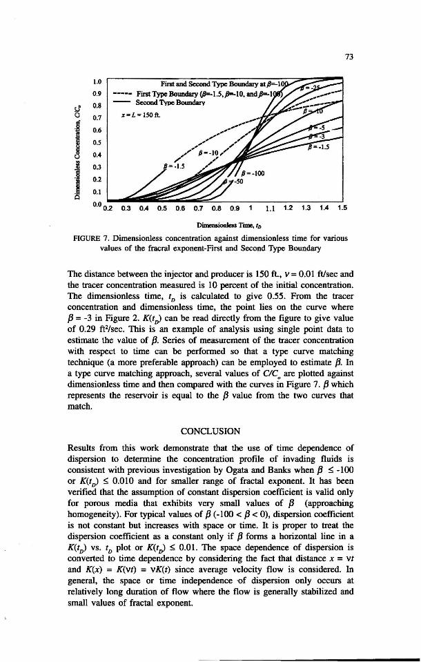
Figure 7 is generated from the equation utilizing the second type boundary. It can be observed that the solution employing the second type boundary condition becomes closer to the solution employing the ftrst type boundary condition as the value of b decreases. For a perfectly homogeneous reservoir, both solutions become the same. For a heterogeneous reservoir, the solution employing the second boundary condition yields lower values of dimensionless concentration than the solution employing the first boundary condition.

APPROXIMATION OF FRACTAL EXPONENT TO DETERMINE DISPERSION COEFFICIENT

It is possible to estimate the value of f3 from a tracer test by measuring the tracer concentration at the producing well with time. The average fluid velocity can be obtained from a tracer analysis. Considering that the tracer concentration measured at the producing well takes approximately 2.3 hours.

1.0

0.9

~ 0.8 5 0.7

·f 0.6

J 0.5

0.4

j 0.3

.1 0.2

0.1 Q

0.0 0.2

First and Second Type Boundary atP=-l ----- First Type BoundaIy (,8=-l.S,P=-IO, andP=-1 -- Second Type Boundary

73

0.3 0.4 0.5 0.6 0.7 0.8 0.9 1.1 1.2 1.3 1.4 1.5

Dimensionless Time, tD

FIGURE 7. Dimensionless concentration against dimensionless time for various values of the fracral exponent-First and Second Type Boundary

The distance between the injector and producer is 150 ft., v = 0.01 ft/sec and the tracer concentration measured is 10 percent of the initial concentration. The dimensionless time, tD is calculated to give 0.55. From the tracer concentration and dimensionless time, the point lies on the curve where fl = -3 in Figure 2. K(tol can be read directly from the figure to give value of 0.29 ft2/sec. This is an example of analysis using single point data to estimate the value of fl. Series of measurement of the tracer concentration with respect to time can be performed so that a type curve matching technique (a more preferable approach) can be employed to estimate fl. In a type curve matching approach, several values of CIC

o are plotted against

dimensionless time and then compared with the curves in Figure 7. fl which represents the reservoir is equal to the fl value from the two curves that match.

CONCLUSION

Results from this work demonstrate that the use of time dependence of dispersion to determine the concentration profile of invading fluids is consistent with previous investigation by Ogata and Banks when fl ~ -100 or K(tol ~ 0.010 and for smaller range of fractal exponent. It has been verified that the assumption of constant dispersion coefficient is valid only for porous media that exhibits very small values of fl (approaching homogeneity). For typical values of fl (-100 < fl < 0), dispersion coefficient is not constant but increases with space or time. It is proper to treat the dispersion coefficient as a constant only if fl forms a horizontal line in a K(tD) vs. tD plot or K(tol ~ 0.01. The space dependence of dispersion is converted to time dependence by considering the fact that distance x = vt

and K(x) = K(vt) = vK(t) since average velocity flow is considered. In general, the space or time independence -of dispersion only occurs at relatively long duration of flow where the flow is generally stabilized and small values of fractal exponent.

74

REFERENCES

Bear, J. 1972. Dynamics of flow in porous media. New York :American Elsevier Publishing Co.

Brigham, W. E., & Abbaszadeh-Dehghani, M. 1987. Tracer testing for reservoir description. J. Pet. Tech. 246(8): 519-527.

Erkal, A. 1997. An analytical solution for non-fickian advection-dispersion equation: effects on dnapl pool dissolution. PhD Dissertation, University of Missouri­Rolla.

Fetter, C. W. 1993. Contaminant hydrogeology. New York: Macmillan Publishing Company, 56-90.

Lake, L. W. 1989. Enhanced oil recovery. New Jersey : Prentice Hall Inc, 157-164. Luster, G. R. 1986. Raw material for portland cement: application of conditional

simulation or coregionalization. PhD Dissertation, Stanford University, Stanford. Marie, C. M. 1980. Multiphase flow in porous medium. Houston: Gulf Publishing. Mishra, S., Brigham, W. E., & Orr Jr., E M. 1991. Tracer and pressure test

analysis for characterization of areally heterogeneous reservoirs. Soc. Pet. Engrs. J. 22(4): 479-489.

Ogata, A., & Banks, R.B. 1964. A solution of the differential equation of longitudinal dispersion in porous media. Appl. Phys. J. 90(1): 13-31.

Pickens, J. E, & Grisak, G. E. 1981. Scale dependent dispersion in a stratified granular aquifer Water Resources Res. 17(3): 529-544.

Sauty, J.-P. 1980. An analysis of hydrodispersive transfer in aquifers. Water Resources Res. 16(1): 145-58.

Stalkup Jr., E 1983. Miscible displacement. Soc. Pet. Engrs. Monograph 8(7): 35-37.

Streltsova, T. D. 1988. Well testing in heterogeneous formations. New York: John Wiley & Sons.

Sudicky, E. A. 1986. A natural gradient experiment on solute transport in a sand aquifer: spatial variability of hydraulic conductivity and its role in the dispersion process. Water Resources Res. 22(13): 2069-2082.

Zhang, Q. 1991. A multi-length scale theory of the anomalous mixing-length growth for tracer flow in heterogeneous porous media. J. Statistical Phys. 66: 485-499.

Mohd.Roslee Othman School of Chemical Engineering Universiti Sains Malaysia 14300 Nibong Tebal, Pulau Pinang Malaysia

D.T. Numbere Department of Petroleum Engineering University of Missouri-Rolla 65401 Missouri, United States of America Email: chroslee@eng.usm.my