Luz e Luz e ÁÁtomostomos comocomo ferramentasferramentas

parapara InformaInformaççãoão QuânticaQuântica

ÓÓticatica QuânticaQuântica

Marcelo MartinelliInst. de

Física

Lab. de Manipulação Coerente de Átomos e Luz

QuestionQuestion::

Dividing the incident beam in two “equal” parts, what will be the result?

i1

i2 -

PBSW

?isub

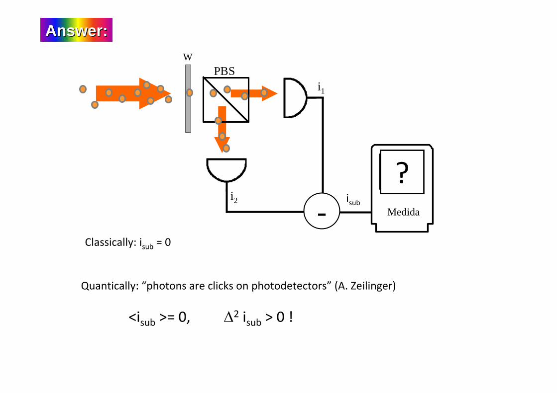
AnswerAnswer::

i1

i2 - Medida

PBSW

?isub

Classically: isub = 0  

Quantically: “photons are clicks on photodetectors” (A. Zeilinger)

<isub >= 0,  ∆2 isub > 0 !

Quantum Quantum MechanicsMechanicsBirth of a revolution at the dawn of the 20th Century

Introduction of theconcept of “quanta”

Quantum Quantum OpticsOptics

Quantization of the Electromagnetic Field (on the shoulders...)

Quantum Quantum OpticsOptics

Maxwell Equations

Wavevector

PolarizationAmplitude

Angular Frequency

OpticsOptics

Solution in a Box

Quantum Quantum OpticsOpticsOpticsOptics

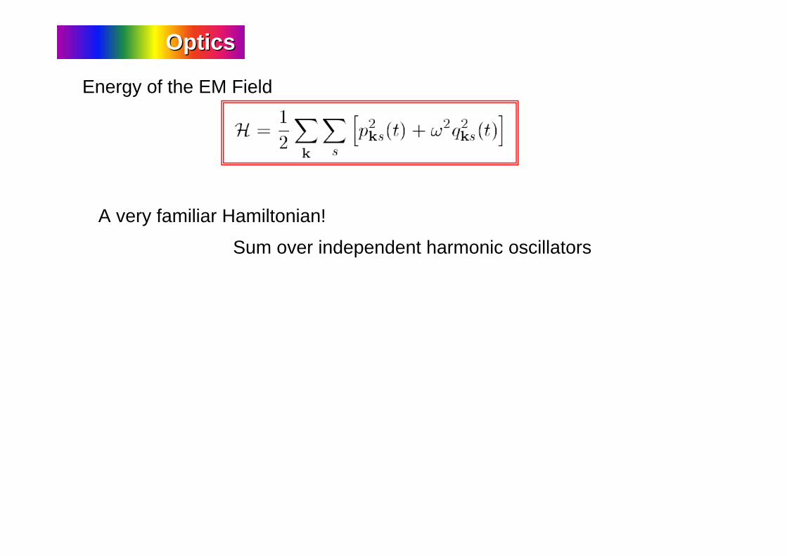
Energy of the EM Field

Canonical Variables: going into Hamiltonian formalism

Quantum Quantum OpticsOpticsOpticsOptics

Energy of the EM Field

Canonical Variables: going into Hamiltonian formalism

Quantum Quantum OpticsOpticsOpticsOptics

Energy of the EM Field

A very familiar Hamiltonian!

Sum over independent harmonic oscillators

Quantum Quantum OpticsOptics

Energy of the EM Field

Using creation and annihilation operators, associated with amplitudes uks

Amplitudes of Electric and Magnetic Fields

Quantum Quantum OpticsOptics

Energy of the EM Field

• Classical Description of the Electromagnectic Field:

Fresnel Representation of a single mode

E(t)=Re{α exp[i(k⋅r ‐ ωt)]}

Field Quadratures Field Quadratures –– Classical DescriptionClassical Description

E(t)=Re[α exp(iωt)]

E(t)=X cos(ωt)+ Y sen(ωt)

α = X + i Y

X

Y

φ

|α |

Field Quadratures Field Quadratures –– Classical DescriptionClassical Description

For a fixed position

• Classical Description of the Electromagnectic Field:

Fresnel Representation of a single mode

The electric field can be decomposed as

And also as

X and Y are the field quadrature operators, satisfying

Thus,

Field Quadratures Field Quadratures –– Quantum OpticsQuantum Optics

X

Y

φ

|α |

Field Quadratures Field Quadratures –– Quantum OpticsQuantum Optics

Thus,

Uncertainty relation implies in a

probability distribution for a given

pair of quadrature measurements

Field quadratures behave just as position and momentum operators!

Quantum OpticsQuantum Optics

Now we know that:- the description of the EM field follows that of a set of

harmonic oscillators, - the quadratures of the electric field are observables, and - they must satisfy an uncertainty relation.

But how to describe different states of the EM field?

Can we find appropriate basis for the description of the field?

Or alternatively, can we describe it using density operators?

And how to characterize these states?

Quantum Optics Quantum Optics –– Number StatesNumber StatesEigenstates of the number operator

Number of excitations in a given harmonic oscillator

number of excitations in a given mode of the field

number of photons in a given mode!

Annihilation and creation operators:Fock States:Eigenvectors of the Hamiltonian

Quantum Optics Quantum Optics –– Number StatesNumber States

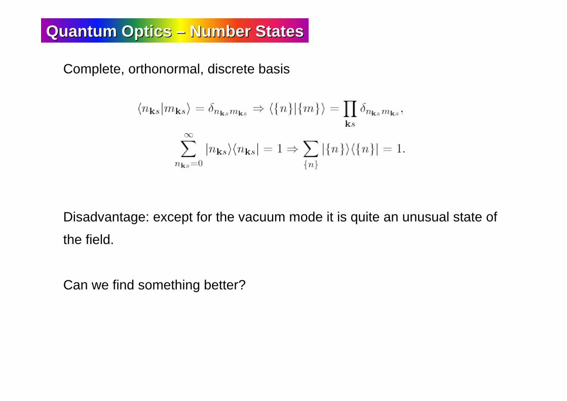
Complete, orthonormal, discrete basis

Disadvantage: except for the vacuum mode it is quite an unusual state of

the field.

Can we find something better?

Quantum Optics Quantum Optics –– Coherent StatesCoherent States

Eigenvalues of the annihilation operator:

In the Fock State Basis:

Completeness: but is not orthonormal

Over-complete!

Moreover:

- corresponds to the state generated by a classical current,

- reasonably describes a monomode laser well above threshold,

- it is the closest description of a “classical” state.

Quantum Optics Quantum Optics –– Number StatesNumber States

0

1

2

Precise number of photons

Growing dispersion of the quadratures

Quantum Optics Quantum Optics –– Number StatesNumber StatesQuantum Optics Quantum Optics –– Coherent StateCoherent State

0

1

2

+

+

+

+

Poissonian distribution of photons

Quantum Optics Quantum Optics –– Coherent StateCoherent State

0

1

2Mean value of number operator

Therefore, variance of photon number is equal to the mean number!

X

Y

φ

|α |

Quantum Optics Quantum Optics –– Coherent StateCoherent State

X

Y

Quantum Optics Quantum Optics –– Coherent Squeezed StatesCoherent Squeezed States

φ

|α |

Coherent States

P(α) : representation of the density operator: Glauber and Sudarshan

Quantum Optics Quantum Optics –– Density OperatorsDensity OperatorsStatistical mixture of pure states

Coherent States

P(α) : representation of the density operator: Glauber and Sudarshan

Quantum Optics Quantum Optics –– Density OperatorsDensity Operators

Representations of the density operators provide a simple way

to describe the state of the field as a function of dimension 2N, where

N is the number of modes involved.

P representation is a good way to present “classical” states,

like thermal light or coherent states.

But it is singular for “non classical states” (e.g. Fock and

squeezed states).

We will see some other useful representations, but for the

moment, how can we get information from the state of the field?

Quantum Optics Quantum Optics –– Measurement of the FieldMeasurement of the FieldSlow varying EM Field can be detected by an antenna:

conversion of electric field in electronic displacement.

amplification, recording, analysis of the signal.

electronic readly available.

Example: 3 K cosmic background (Penzias & Wilson).

Problems:

Even this tiny field accounts for a strong photon

density.

Every measurement needs to account for thermal

background (e.g. Haroche et al.).

Quantum Optics Quantum Optics –– Measurement of the FieldMeasurement of the FieldFast varying EM Field cannot be measured directly.

We often detect the mean value of the Poynting vector:

Photoelectric effect converts photons into ejected electrons

We measure photo-electrons

individually with APDs or photomultipliers – a single electron is converted in a

strong pulse – discrete variable domain,

in a strong flux with photodiodes, where the photocurrent is converted into a

voltage – continuous variable domain.

Advantages: in this domain, photons are energetic enough:

in a small flux, every photon counts.

for the eV region (visible and NIR), presence of background photons is

negligible: measurements are nearly the same in L-He or at room temperature.

Quantum Optics Quantum Optics –– Measurement of the FieldMeasurement of the Field

And detectors are cheap!

Ê

Quantum Optics Quantum Optics –– Measurement of the Measurement of the IntenseIntense FieldField

We can easily measure photon flux: field intensity

(or more appropriate, optical power)

OK, we got the amplitude measurement, but that is only part of the history!

Amplitude is directly related to the measurement of the number of

photon, (or the photon counting rate, if you wish).

This leaves an unmeasured quadrature, that can be related to the

phase of the field.

But there is not such an evident “phase operator”!

Still, there is a way to convert phase into amplitude: interference

and interferometers.

Quantum Optics Quantum Optics –– Measurement of the FieldMeasurement of the FieldQuantum Optics Quantum Optics –– Measurement of the Measurement of the IntenseIntense FieldField

Michelson or Mach Zender demonstration

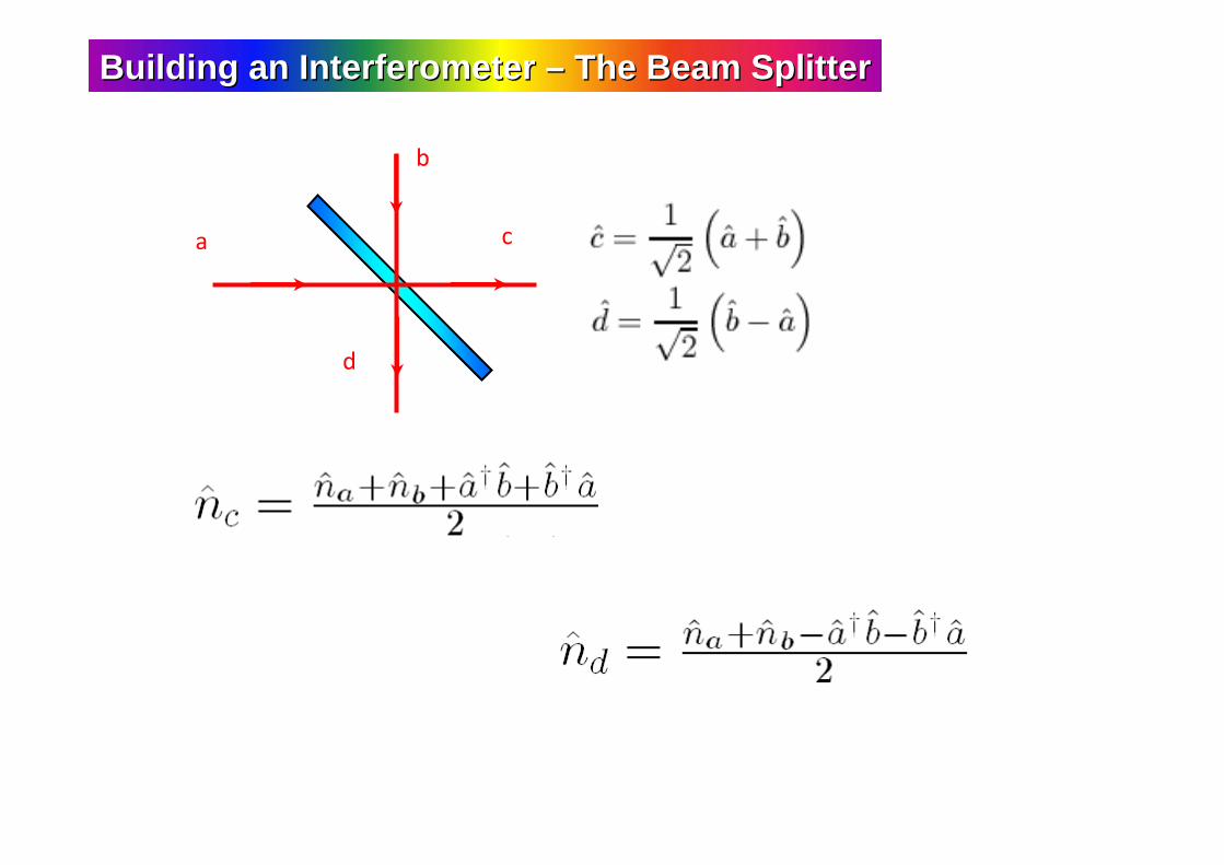
a

b

d

c

Building an Interferometer Building an Interferometer –– The Beam SplitterThe Beam Splitter

±

BS

D2

D1b

c

d

A

Homodyning if <|  |>  <<  <|  |>  

Vacuum HomodyningCalibration of the Standard Quantum Level

Building an Interferometer Building an Interferometer –– The Beam SplitterThe Beam Splitter

“Classical” VarianceShot noise !

Vacuum Homodyning allows the calibration of the detection, producing a Poissoniandistribution in the output (just like a coherent state).