lyapunov inverse iteration for computing a few rightmost

University of Maryland Department of Computer Science TR-5009University of Maryland Institute for Advanced Computer Studies TR-2012-07

April 2012

LYAPUNOV INVERSE ITERATION FOR COMPUTING A FEW RIGHTMOSTEIGENVALUES OF LARGE GENERALIZED EIGENVALUE PROBLEMS∗

HOWARD C. ELMAN† AND MINGHAO WU‡

Abstract. In linear stability analysis of a large-scale dynamical system, we need to compute the rightmosteigenvalue(s) for a series of large generalized eigenvalue problems. Existing iterative eigenvalue solvers are not robustwhen no estimate of the rightmost eigenvalue(s) is available. In this study, we show that such an estimate can beobtained from Lyapunov inverse iteration applied to a special eigenvalue problem of Lyapunov structure. We alsoshow that Lyapunov inverse iteration will always converge in only two steps if the Lyapunov equation in the firststep is solved accurately enough. Furthermore, we generalize the analysis to a deflated version of this Lyapunoveigenvalue problem and propose an algorithm that computes a few rightmost eigenvalues for the eigenvalue problemsarising from linear stability analysis. Numerical experiments demonstrate the robustness of the algorithm.

1. Introduction. This paper introduces an efficient algorithm for computing a few rightmosteigenvalues of generalized eigenvalue problems. We are concerned with problems of the form

J (α)x = µMx (1.1)

arising from linear stability analysis (see [11]) of the dynamical system

Mut = f(u, α). (1.2)

M ∈ Rn×n is called the mass matrix, and the parameter-dependent matrix J (α) ∈ Rn×n isthe Jacobian matrix ∂f

∂u (u(α), α) = ∂f∂u (α), where u(α) is the steady-state solution to (1.2) at

α, i.e., f(u, α) = 0. Let the solution path be the following set: S = {(u, α)|f(u, α) = 0}. Weseek the critical point (uc, αc) associated with transition to instability on S. While the methoddeveloped in this study works for any dynamical system of the form (1.2), our primary interest isthe ones arising from spatial discretization of 2- or 3-dimensional time-dependent partial differentialequations (PDEs). Therefore, we assume n to be large and J (α),M to be sparse throughout thispaper.

The conventional method of locating the critical parameter αc is to monitor the rightmosteigenvalue(s) of (1.1) while marching along S using numerical continuation (see [11]). In the stableregime of S, the eigenvalues µ of (1.1) all lie to the left of the imaginary axis. As (u, α) approachesthe critical point, the rightmost eigenvalue of (1.1) moves towards the imaginary axis; at (uc, αc), therightmost eigenvalue of (1.1) has real part zero, and finally, in the unstable regime, some eigenvaluesof (1.1) have positive real parts. The continuation usually starts from a point (u0, α0) in the stableregime of S and the critical point is detected when the real part of the rightmost eigenvalue of(1.1) becomes nonnegative. Consequently, robustness and efficiency of the eigenvalue solver for therightmost eigenvalue(s) of (1.1) are crucial for the performance of this method. Direct eigenvalue

∗This work was supported in part by the U. S. Department of Energy under grant DEFG0204ER25619 and theU. S. National Science Foundation under grant DMS1115317.†Department of Computer Science and Institute for Advanced Computer Studies, University of Maryland, College

Park, MD 20742 ([email protected]).‡Applied Mathematics & Statistics, and Scientific Computation Program, Department of Mathematics, University

of Maryland, College Park, MD 20742 ([email protected]).

1

solvers such as the QR and QZ algorithms (see [20]) compute all the eigenvalues of (1.1), but theyare too expensive for large n. Existing iterative eigenvalue solvers [20] are able to compute a smallset (k � n) of eigenvalues of (1.1) near a given shift (or target) σ ∈ C efficiently. For example, theywork well when k eigenvalues of (1.1) with smallest modulus are sought, in which case σ = 0. Oneissue with such methods is that there is no robust way to determine a good choice of σ when we haveno idea where the target eigenvalues may be. In the computation of the rightmost eigenvalue(s),the most commonly used heuristic choice for σ is zero, i.e., we compute k eigenvalues of (1.1) withsmallest modulus and hope that the rightmost one is one of them. When the rightmost eigenvalue isreal, zero is a good choice. However, such an approach is not robust when the rightmost eigenvaluesconsist of a complex conjugate pair: the rightmost pair can be far away from zero and it is not clearhow big k should be to ensure that they are found. Such examples can be found in the numericalexperiments of this study.

Meerbergen and Spence [15] proposed the Lyapunov inverse iteration method, which estimatesthe critical parameter αc without computing the rightmost eigenvalues of (1.1). Assume (u0, α0)is in the stable regime of S and is also in the neighborhood of the critical point (uc, αc). Letλc = αc − α0 and A = J (α0). Then the Jacobian matrix J (αc) at the critical point can beapproximated by A + λcB where B = dJ

dα (α0). It is shown in [15] that λc is the eigenvalue withsmallest modulus of the eigenvalue problem

AZMT + MZAT + λ(BZMT + MZBT ) = 0 (1.3)

of Lyapunov structure and that λc can be computed by a matrix version of inverse iteration.Estimates of the rightmost eigenvalue(s) of (1.1) at αc can be obtained as by-products. Elmanet al. [8] refined the Lyapunov inverse iteration proposed in [15] to make it more robust andefficient and examined its performance on challenging test problems arising from fluid dynamics.Various implementation issues were discussed, including the use of inexact inner iterations, theimpact of the choice of iterative method used to solve the Lyapunov equations, and the effect ofeigenvalue distribution on performance. Numerical experiments demonstrated the robustness oftheir algorithm.

The method proposed in [8, 15], although it allows us to estimate the critical value of theparameter without computing the rightmost eigenvalue(s) of (1.1), only works in the neighborhoodof the critical point (uc, αc). In [8], for instance, the critical parameter value αc of all numericalexamples is known a priori, so that we can pick a point (u0, α0) close to (uc, αc) and apply Lyapunovinverse iteration with confidence. In reality, αc is unknown and we start from a point (u0, α0) inthe stable regime of S that may be distant from the critical point. In this scenario, the method of[8, 15] cannot be used to estimate αc, since J (αc) cannot be approximated by A + λcB. However,quantitative information about how far away (u0, α0) is from (uc, αc) can still be obtained byestimating the distance between the rightmost eigenvalue of (1.1) at α0 and the imaginary axis: ifthe rightmost eigenvalue is far away from the imaginary axis, then it is reasonable to assume that(u0, α0) is far away from the critical point as well, and therefore we should march along S usingnumerical continuation until we are close enough to (uc, αc); otherwise, we can assume that (u, α0)is already in the neighborhood of the critical point and the method of [8, 15] can be applied toestimate αc.

The goal of this paper is to develop a robust method to compute a few rightmost eigenvalues of(1.1) in the stable regime of S. The plan of the paper is as follows. In section 2, we show that thedistance between the imaginary axis and the rightmost eigenvalue of (1.1) is the eigenvalue withsmallest modulus of an eigenvalue problem similar in structure to (1.3). As a result, this eigenvalue

2

can be computed efficiently by Lyapunov inverse iteration. In section 3, we present numerical resultsfor several examples arising from fluid dynamics, and provide an analysis of the fast convergence ofLyapunov inverse iteration observed in our experiments. Based on the analysis, we also propose amodified algorithm that guarantees convergence in only two iterations. In section 4, we show thatthe analysis in sections 2 and 3 can be generalized to a deflated version of the Lyapunov eigenvalueproblem, which leads to an algorithm for computing k (1 ≤ k � n) rightmost eigenvalues of (1.1).Details of the implementation of this algorithm are discussed in section 5. Finally, we make someconcluding remarks in section 6.

2. Computing the distance between the rightmost eigenvalue(s) and the imaginaryaxis. Let (u0, α0) be any point in the stable regime of S and assume M is nonsingular in (1.1).Let (µj , xj) (‖xj‖2 = 1, j = 1, 2, . . . , n) be the eigenpairs of (1.1) at α0, where the real partsof µj , Re(µj), are in decreasing order, i.e., 0 > Re(µ1) ≥ Re(µ2) ≥ . . . ≥ Re(µn). Then thedistance between the rightmost eigenvalue(s) and the imaginary axis is −Re(µ1). Let A = J (α0)and S = A−1M. To compute this distance, we first observe that −Re(µ1) is the eigenvalue withsmallest modulus of the n2 × n2 generalized eigenvalue problem

∆1z = λ(−∆0)z (2.1)

where ∆1 = S ⊗ I + I ⊗ S and ∆0 = 2S ⊗ S (I is the identity matrix of order n). We proceed intwo steps to prove this assertion. First, we show that −Re(µ1) is an eigenvalue of (2.1).

Theorem 2.1. The eigenvalues of (2.1) are λi,j = − 12 (µi + µj), i, j = 1, 2, . . . , n. For any

pair (i, j), there are eigenvectors associated with λi,j given by zi,j = xi ⊗ xj and zj,i = xj ⊗ xi.Proof. Since (µj , xj) (j = 1, 2, . . . , n) are the eigenpairs of Ax = µMx,

(1µj, xj

)are the

eigenpairs of S. We first prove that the eigenvalues of (2.1) are {λi,j}ni,j=1. Let J be the Jordan

normal form of S and P be an invertible matrix such that S = PJP−1. Then

(−∆0)−1

∆1(P ⊗ P ) = −1

2(PJP−1 ⊗ PJP−1)−1(PJP−1 ⊗ I + I ⊗ PJP−1)(P ⊗ P )

= −1

2

(PJ−1P−1 ⊗ PJ−1P−1

)(PJ ⊗ P + P ⊗ PJ)

= −1

2(P ⊗ P )

(J−1P−1 ⊗ J−1P−1

)(PJ ⊗ P + P ⊗ PJ)

= (P ⊗ P )

[−1

2

(I ⊗ J−1 + J−1 ⊗ I

)].

This implies that (2.1) and − 12

(I ⊗ J−1 + J−1 ⊗ I

)have the same eigenvalues. Due to the special

structure of the Jordan normal form J , I ⊗ J−1 + J−1 ⊗ I is an upper triangular matrix whosediagonal entries are {µi + µj}ni,j=1. Consequently, the eigenvalues of − 1

2

(I ⊗ J−1 + J−1 ⊗ I

)are{

− 12 (µi + µj)

}ni,j=1

= {λi,j}ni,j=1. Therefore, the eigenvalues of (2.1) are {λi,j}ni,j=1 as well.

Second, we show that zi,j is an eigenvector of (2.1) associated with the eigenvalue λi,j . For anypair (i, j) (i, j = 1, 2, . . . , n),

∆1(xi ⊗ xj) = (S ⊗ I + I ⊗ S)(xi ⊗ xj) = (Sxi)⊗ xj + xi ⊗ (Sxj) =

(1

µi+

1

µj

)(xi ⊗ xj),

and

∆0(xi ⊗ xj) = 2(S ⊗ S)(xi ⊗ xj) = 2(Sxi)⊗ (Sxj) =2

µiµj(xi ⊗ xj).

3

Therefore, ∆1zi,j =(

1µi

+ 1µj

)µiµj

2 ∆0zi,j = λi,j (−∆0) zi,j . Similarly, we can show that ∆1zj,i =

λi,j (−∆0) zj,iIf µ1 is real, then −Re(µ1) = −µ1 = − 1

2 (µ1 + µ1) = λ1,1; if µ1 is not real (i.e., µ1 = µ2 andx1 = x2), then −Re(µ1) = − 1

2 (µ1 + µ1) = − 12 (µ1 + µ2) = λ1,2 = λ2,1. In both cases, by Theorem

2.1, −Re(µ1) is an eigenvalue of (2.1).We next show that −Re(µ1) is the eigenvalue of (2.1) with smallest modulus.Theorem 2.2. Assume all the eigenvalues of Ax = µMx lie in the left half of the complex

plane. Then the eigenvalue of (2.1) with smallest modulus is −Re(µ1).Proof. Let µj = aj + ibj . Then 0 > a1 ≥ a2 ≥ . . . ≥ an. If the rightmost eigenvalue of

Ax = µMx is real, then −Re(µ1) = λ1,1, and since 0 > a1 ≥ a2 ≥ . . . ≥ an, it follows that

|λ1,1|2 =1

4(a1 + a1)2 ≤ 1

4

[(ai + aj)

2 + (bi + bj)2]

= |λi,j |2

for any pair (i, j). Alternatively, if the rightmost eigenvalues of Ax = µMx consist of a complexconjugate pair, then a1 = a2, b1 = −b2, −Re(µ1) = λ1,2 = λ2,1, and similarly,

|λ1,2|2 = |λ2,1|2 =1

4

[(a1 + a1)2 + (b1 − b1)2

]≤ 1

4

[(ai + aj)

2 + (bi + bj)2]

= |λi,j |2

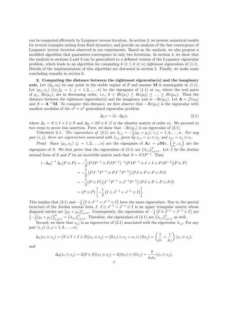
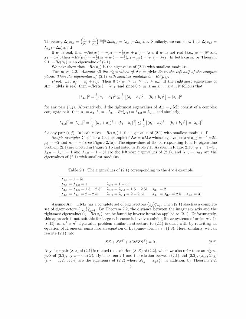
for any pair (i, j). In both cases, −Re(µ1) is the eigenvalue of (2.1) with smallest modulus.Simple example: Consider a 4×4 example of Ax = µMx whose eigenvalues are µ1,2 = −1±5i,

µ3 = −2 and µ4 = −3 (see Figure 2.1a). The eigenvalues of the corresponding 16 × 16 eigenvalueproblem (2.1) are plotted in Figure 2.1b and listed in Table 2.1. As seen in Figure 2.1b, λ1,1 = 1−5i,λ1,2 = λ2,1 = 1 and λ2,2 = 1 + 5i are the leftmost eigenvalues of (2.1), and λ1,2 = λ2,1 are theeigenvalues of (2.1) with smallest modulus.

Table 2.1: The eigenvalues of (2.1) corresponding to the 4× 4 example

λ1,1 = 1− 5iλ2,1 = λ1,2 = 1 λ2,2 = 1 + 5iλ3,1 = λ1,3 = 1.5− 2.5i λ3,2 = λ2,3 = 1.5 + 2.5i λ3,3 = 2λ4,1 = λ1,4 = 2− 2.5i λ4,2 = λ2,4 = 2 + 2.5i λ4,3 = λ3,4 = 2.5 λ4,4 = 3

Assume Ax = µMx has a complete set of eigenvectors {xj}nj=1. Then (2.1) also has a completeset of eigenvectors {zi,j}ni,j=1. By Theorem 2.2, the distance between the imaginary axis and therightmost eigenvalue(s), −Re(µ1), can be found by inverse iteration applied to (2.1). Unfortunately,this approach is not suitable for large n because it involves solving linear systems of order n2. In[8, 15], an n2 × n2 eigenvalue problem similar in structure to (2.1) is dealt with by rewriting anequation of Kronecker sums into an equation of Lyapunov form, i.e., (1.3). Here, similarly, we canrewrite (2.1) into

SZ + ZST + λ(2SZST ) = 0. (2.2)

Any eigenpair (λ, z) of (2.1) is related to a solution (λ, Z) of (2.2), which we also refer to as an eigen-pair of (2.2), by z = vec(Z). By Theorem 2.1 and the relation between (2.1) and (2.2), (λi,j , Zi,j)(i, j = 1, 2, . . . , n) are the eigenpairs of (2.2) where Zi,j = xjx

Ti ; in addition, by Theorem 2.2,

4

−4 −3.5 −3 −2.5 −2 −1.5 −1 −0.5 0−6

−4

−2

0

2

4

6

real axis

imag

inar

y ax

is

(a) The spectrum of Ax = µMx

0 0.5 1 1.5 2 2.5 3 3.5 4−6

−4

−2

0

2

4

6

real axis

imag

inar

y ax

is

(b) The spectrum of (2.1)

Fig. 2.1: The spectrum of Ax = µMx and (2.1) for the 4× 4 example (•: double eigenvalues).

−Re(µ1) is the eigenvalue of (2.2) with smallest modulus. Furthermore, under certain conditions,−Re(µ1) is an eigenvalue of (2.2) whose associated eigenvector is real, symmetric and of low rank.Assume the following: (a1) for any 1 < i ≤ n, if Re(µi) = Re(µ1), then µi = µ1; (a2) µ1 is asimple eigenvalue of Ax = µMx. Consequently, if µ1 is real, −Re(µ1) is a simple eigenvalue of(2.1) with the eigenvector z1,1 = x1 ⊗ x1; otherwise, −Re(µ1) is a double eigenvalue of (2.1) withthe eigenvectors z1,2 = x1⊗ x1 and z2,1 = x1⊗ x1. When the eigenvectors of (2.2) are restricted tothe subspace of Cn×n consisting of symmetric matrices Z, then by Theorem 2.3 from [15], −Re(µ1)has a unique (up to a scalar multiplier), real and symmetric eigenvector x1x

T1 (if µ1 is real), or

x1x∗1 + x1x

T1 (if µ1 is not real) where x∗1 denotes the conjugate transpose of x1. Therefore, we can

apply Lyapunov inverse iteration (see [8,15]) to (2.2) to find −Re(µ1), the eigenvalue of (2.2) withsmallest modulus:

Algorithm 1 (Lyapunov inverse iteration for (2.2))1. Given V0 ∈ Rn with ‖V0‖2 = 1 and d0 = 1.2. For ` = 1, 2, · · ·

2.1. Rank reduction1: compute S = V T`−1SV`−1 and solve for the eigenvalue λ1 of

SZ + ZST + λ(

2SZST)

= 0 (2.3)

with smallest modulus and its eigenvector Z1 = V DV T , where V ∈ Rd`−1×r,D ∈ Rr×r with ‖D‖F = 1, and r = 1 (` = 1) or 2 (` ≥ 2).

2.2. Set λ(`) = λ1 and Z(`) = V`DVT` , where V` = V`−1V .2.3. If

(λ(`), Z(`)

)is accurate enough, then stop.

2.4. Else, solve for Y` from

SY` + Y`ST = −2SZ(`)ST (2.4)

1When ` = 1, (2.3) is a scalar equation and its eigenpair is(λ1, Z1

)=(−S−1, 1

).

5

in factored form: Y` = V`D`VT` , where V` ∈ Rn×d` is orthonormal and D` ∈ Rd`×d` .

As the iteration proceeds, the iterate(λ(`), Z(`) = V`DVT`

)will converge to (−Re(µ1),VDVT )

where ‖D‖F = 1 and V = x1 (if µ1 is real) or V ∈ Rn×2 is an orthonormal matrix whose columnsspan {x1, x1} (if µ1 is not real). Besides estimates of −Re(µ1), we can also obtain from Algorithm1 estimates of (µ1, x1) by solving the small 1× 1 or 2× 2 eigenvalue problem(

VT` SV`)y = θy (2.5)

and taking µ(`) = 1θ and x(`) = V`y. As V` converges to V,

(µ(`), x(`)

)will converge to (µ1, x1).

At each iteration of Algorithm 1, a large-scale Lyapunov equation (2.4) needs to be solved. Wecan rewrite (2.4) as

SY` + Y`ST = P`C`P

T` (2.6)

(see [8] for details) where P` is orthonormal and is of rank 1 (` = 1) or 2 (` > 1). The solution to(2.6), Y`, is real and symmetric and frequently has low rank (see [1, 16]). Since S is large, directmethods such as [2,12] are not suitable. An iterative method that solves Lyapunov equations withlarge coefficient matrix and low-rank right-hand side is needed. Krylov-type methods for (2.6),such as the “standard” Krylov subspace method [13, 17], the Extended Krylov Subspace Method(EKSM) [18] and the Rational Krylov Subspace Method (RKSM) [6, 7], construct approximatesolutions of the form Y approx` = WXWT where W is an orthonormal matrix whose columns spanthe Krylov subspace and X is the solution to the small, projected Lyapunov equation (WTSW )X+X(WTSW )T = (WTP`)C`(W

TP`)T , which can be obtained using direct methods. For example,

the standard Krylov subspace method [13,17] builds the mp-dimensional Krylov subspace

Km(S, P`) = span{P`, SP`, . . . , S

m−1P`}

(2.7)

where m is the number of block Arnoldi steps and p is the block size (i.e., rank of P`). The maincost of solving (2.6) using Krylov-type methods is (m − 1)p linear solves with coefficient matrixaA + bM, where values of the scalars a, b depend on the Krylov method used.

In step 2.1 (rank reduction) of Algorithm 1, although it may look like computing the reduced-

rank matrix S = V T`−1SV`−1 requires another d`−1 linear solves with coefficient matrix A, in fact,

if a Krylov-type method is used to solve (2.6), S can be obtained from the Arnoldi decompositioncomputed by the Krylov-type method for no additional cost when ` > 1. Assume the standardKrylov method is used to solve (2.6). In the (` − 1)st iteration of Algorithm 1, it computes theArnoldi decomposition

SV`−1 = V`−1Hm +Wm+1Hm+1,mETm (2.8)

and the approximate solution Y approx1 = V`−1D`−1VT`−1, where the columns of V`−1 form an or-

thonormal basis for the Krylov subspace Km(S, P`−1) and are orthogonal to Wm+1. (In addition,Hm ∈ Rmr×mr is block upper Hessenberg, Wm+1 ∈ Rn×r is orthonormal, Hm+1,m ∈ Rr×r andEm holds the last r columns of the identity matrix of order mr, where r = 1 or 2.) This implies

that in the `th iteration of Algorithm 1, S is simply Hm, which has been computed already. TheArnoldi decomposition computed by EKSM or RKSM has a form that is more complicated than(2.8); nonetheless, it produces the matrix S needed for the next iteration as well.

6

3. Numerical experiments. In this section, we test Algorithm 1 on several problems arisingfrom fluid dynamics. Note that when (1.2) comes from a standard (e.g., finite element) discretizationof the imcompressible Navier-Stokes equations, the mass matrix M is singular, leading to infiniteeigenvalues of (1.1) and singular S = A−1M. As in [8], we use the shifted, nonsingular mass matrixproposed in [4], which maps the infinite eigenvalues of (1.1) to finite ones away from the imaginaryaxis and leaves the finite eigenvalues of (1.1) unchanged. From here on, M refers to this shiftedmass matrix.

3.1. Example 1: driven-cavity flow. Linear stability analysis of this flow is studied in manypapers, for example, [9]. The Q2-Q1 mixed finite element discretization (with a 64 × 64 mesh) ofthe Navier-Stokes equations gives rise to a generalized eigenvalue problem (1.1) of order n = 9539,where the parameter α is the Reynolds number (denoted by Re) of the flow. (The Reynolds numberof this flow is defined to be Re = 1

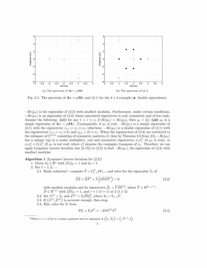
ν , where ν is the kinematic viscosity). Figure 3.1a depicts thepath traced out by the eight rightmost eigenvalues of (1.1) for Re = 2000, 4000, 6000, 7800, at whichthe steady-state solution to (1.2) is stable. As the Reynolds number increases, the following trendcan be observed: the eight rightmost eigenvalues all move towards the imaginary axis, and theybecome more clustered as they approach the imaginary axis. In addition, although the rightmosteigenvalue starts off being real, one conjugate pair of complex eigenvalues (whose imaginary partsare about ±3i) move faster towards the imaginary axis than the other eigenvalues and eventuallythey become the rightmost. They first cross the imaginary axis at Re ≈ 7929, causing instabilityin the steady-state solution of (1.2) (see [8]).

Finding the conjugate pair of rightmost eigenvalues of (1.1) at a high Reynolds number (forexample, at Re = 7800) can be difficult. Suppose we are trying to find the rightmost eigenvaluesat Re = 7800 by conventional methods, such as computing k eigenvalues of (1.1) with smallestmodulus using the Implicitly Restarted Arnoldi (IRA) method [19]. If we use the Matlab function‘eigs’ (which implements the IRA method) with its default setting, then k has to be as large as250, since there are many eigenvalues that have smaller modulus than the rightmost pair. Thisleads to at least 500 linear solves (with coefficient matrix A), and in practice, many more. Moreimportantly, note that the decision k = 250 is made based on a priori knowledge of where therightmost eigenvalues lie. In general, we cannot identify a good value for k that guarantees thatthe rightmost eigenvalues will be found.

For four various Reynolds numbers between 2000 and 7800, we apply Algorithm 1 (with RKSMas the Lyapunov solver) to calculate the distance between the rightmost eigenvalue(s) of (1.1) andthe imaginary axis. The results are reported in Table 3.2 (see Table 3.1 for notation). The initialguess V0 is chosen to be a random vector of unit norm in Rn, the stopping criterion for the eigenvalueresidual is ‖R`‖F < 10−8, and the stopping criterion for the Lyapunov solve is

‖R`‖F < 10−9 ·∥∥P`C`PT` ∥∥F = 10−9 · ‖C`‖F .

Note that both residual norms ‖R`‖F and ‖R`‖F are cheap to compute (see [8] for details). There-fore, the main cost of each iteration is about d` linear solves of order n. All linear systems are solvedusing direct methods. As shown in Table 3.2, the distances between the rightmost eigenvalue(s) of(1.1) and the imaginary axis at Re = 2000, 4000, 6000, 7800 are 0.03264, 0.01608, 0.01084, 0.00514,respectively. We also obtain estimates of the rightmost eigenvalue of (1.1) at the four Reynoldsnumbers: -0.03264, -0.01608, -0.01084, and -0.00514+2.69845i.

We note two trends seen in these results. First, surprisingly, for all the Reynolds numbersconsidered, Algorithm 1 converges to the desired tolerance (‖R`‖F < 10−8) in only 2 iterations.

7

−0.2 −0.15 −0.1 −0.05 0−3

−2

−1

0

1

2

3

real axis

imag

inar

y ax

is

(a)

−3 −2.5 −2 −1.5 −1 −0.5 0−3

−2

−1

0

1

2

3

real axis

imag

inar

y ax

is

(b)

Fig. 3.1: (a) The eight rightmost eigenvalues for driven-cavity flow at different Reynolds numbers(∗ : Re = 2000, ◦ : Re = 4000, ♦ : Re = 6000, � : Re = 7800). (b) The 300 eigenvalues with

smallest modulus at Re = 7800 (×: the rightmost eigenvalues).

Table 3.1: Notation for Algorithm 1

Symbol Definition

λ(`) the estimate of −Re(µ1), i.e., the eigenvalue of (2.2) with smallest modulus

Z(`) the estimated eigenvector of (2.2) associated with −Re(µ1)

µ(`) the estimated rightmost eigenvalue of Ax = µMx computed from (2.5)Y approx` the approximate solution to the Lyapunov solution (2.6)

R`SZ(`) + Z(`)ST + λ(`)(2SZ(`)ST ), the residual of the Lyapunov eigenvalueproblem (2.2)

R` SY approx` + Y approx` ST − P`C`PT` , the residual of the Lyapunov equation (2.6)d` dimension of the Krylov subspace, i.e., rank of Y approx`

That is, only the first Lyapunov equation

SY1 + Y1ST = P1C1P

T1 (3.1)

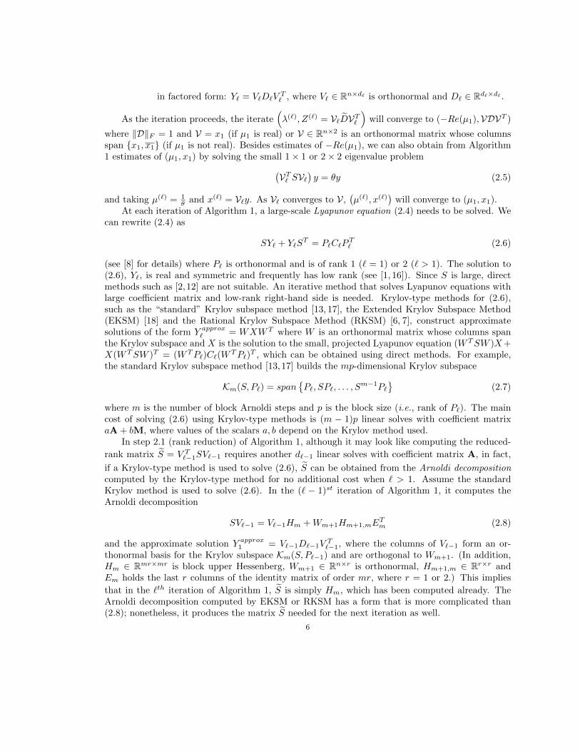
needs to be solved, where P1 ∈ Rn and C1 ∈ R. Second, as the Reynolds number increases, itbecomes more expensive to solve the Lyapunov equation to the same order of accuracy (‖R`‖F <10−9 · ‖C`‖F ), since Krylov subspaces of increasing dimension are needed (156, 241, 307 and 366 forthe four Reynolds numbers). We also tested Algorithm 1 using the standard Krylov method [17] tosolve the Lyapunov systems. To solve (3.1) to the same accuracy, this method requires subspacesof dimension 525, 614, 770 and 896 for the four Reynolds numbers, which are much larger thanthose required by RKSM (see Figure 3.2 for comparison). As a result, the standard method requiresmany more linear solves.

8

Table 3.2: Algorithm 1 applied to Example 1 (Lyapunov solver: RKSM)

` λ(`) µ(`) ‖R`‖F ‖R`‖F d`Re=2000

1 884.383 -884.383 1.32049e+02 1.40794e-10 1562 0.03264 -0.03264 2.56263e-11 — —

Re=40001 -17765.8 17765.8 6.58651e+03 3.52618e-10 2412 0.01608 -0.01608 4.25055e-10 — —

Re=60001 1301.24 -1301.24 8.55652e+02 6.52387e-10 3072 0.01084 -0.01084 7.11628e-10 — —

Re=78001 695.951 -695.951 6.58622e+02 9.02875e-10 3662 0.00514 -0.00514+2.69845i 3.62567e-11 — —

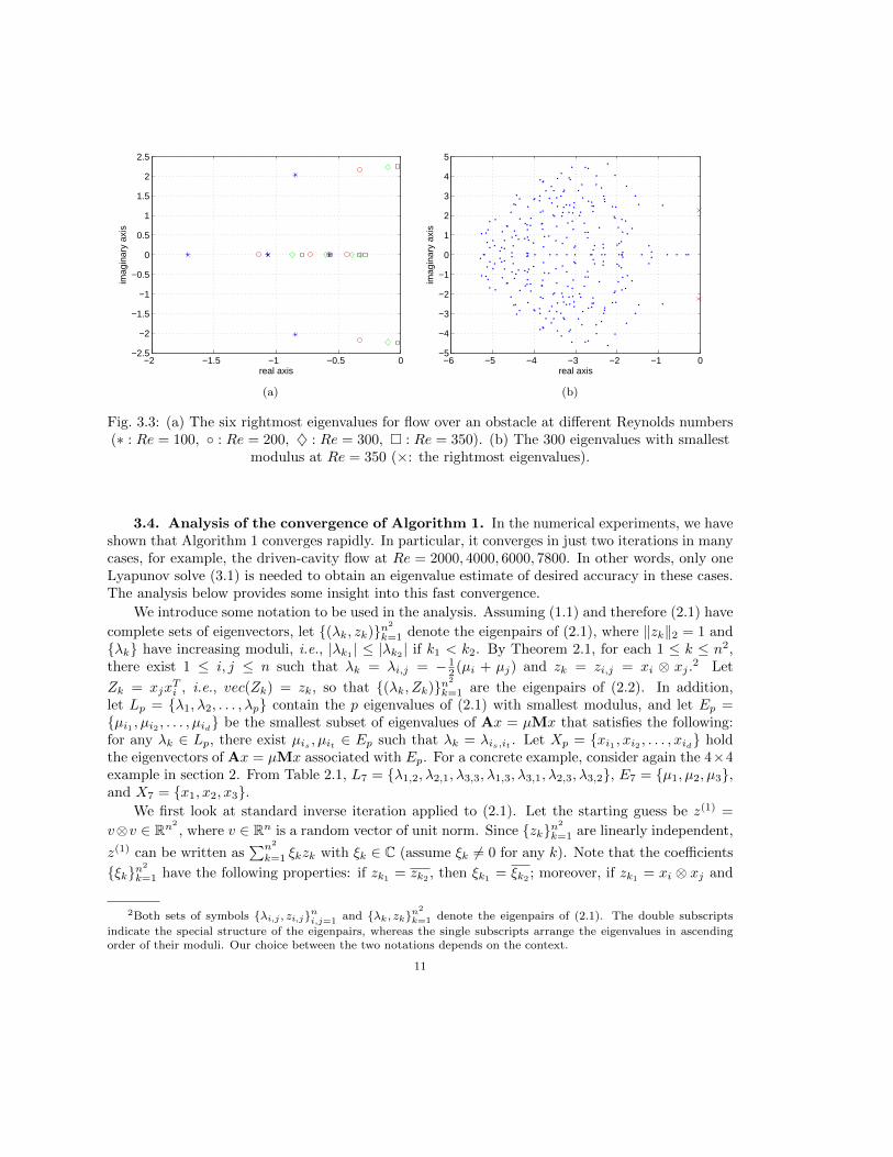
3.2. Example 2: flow over an obstacle. For linear stability analysis of this flow, see[8]. The Q2-Q1 mixed finite element discretization (with a 32 × 128 mesh) of the Navier-Stokesequations gives rise to a generalized eigenvalue problem (1.1) of order n = 9512. Figure 3.3adepicts the path traced out by the six rightmost eigenvalues of (1.1) for Re = 100, 200, 300, 350in the stable regime, and Figure 3.3b shows the 300 eigenvalues of (1.1) with smallest modulus atRe = 350. (In this example, the Reynolds number Re = 2

ν .) As for the previous example, as theReynolds number increases, the six rightmost eigenvalues all move towards the imaginary axis, andthe rightmost eigenvalue changes from being real (at Re = 100) to complex (at Re = 200, 300, 350).The rightmost pair of eigenvalues of (1.1) cross the imaginary axis and the steady-state solution to(1.2) loses its stability at Re ≈ 373.

We again apply Algorithm 1 to estimate the distance between the rightmost eigenvalue(s) of(1.1) and the imaginary axis for the four Reynolds numbers mentioned above. The results arereported in Table 3.3. The stopping criteria for both Algorithm 1 and the Lyapunov solve (2.6)remain unchanged, i.e., ‖R`‖F < 10−8 and ‖R`‖F < 10−9 · ‖C`‖F . For all four Reynolds numbers,Algorithm 1 converges rapidly. In fact, we will show in section 3.4 that if the Lyapunov equation(3.1) is solved more accurately, Algorithm 1 will converge in two iterations in all four cases asobserved in the previous example. Again we compare the performance of the standard Krylovmethod and RKSM in solving (3.1). As for the cavity flow, the Krylov method needs a significantlylarger subspace than RKSM to compute a solution of the same accuracy (see Figure 3.4).

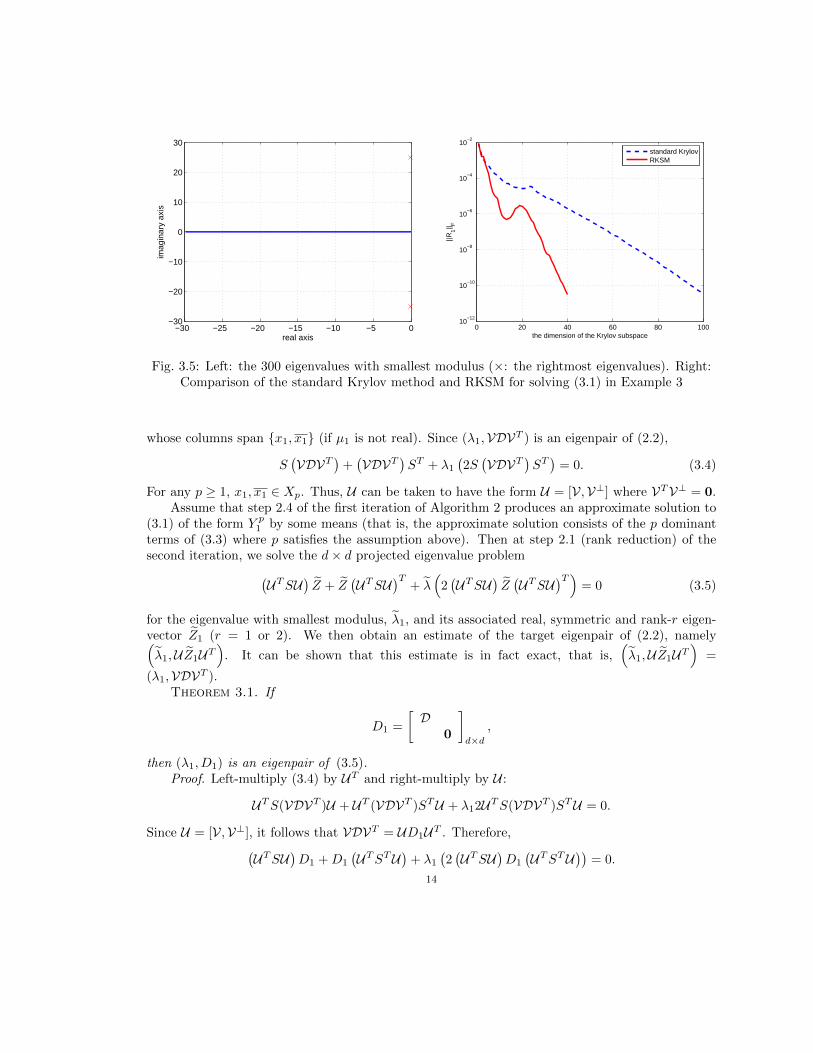
3.3. Example 3: double-diffusive convection problem. This is a model of the effects ofconvection and diffusion on two solutions in a box heated at one boundary (see Chapter 8 of [21]).The governing equations use Boussinesq approximation and are given in [3] and [5]. Linear stabilityanalysis of this problem is considered in [10]. The imaginary parts of the rightmost eigenvaluesof (1.1) near the critical point (uc, αc) have fairly large magnitude, and as a result, the rightmosteigenvalues are further away from zero than many of the real eigenvalues close to the imaginaryaxis. Conventional methods, such as IRA with a zero shift, tend to converge to the real eigenvaluesclose to the imaginary axis instead of the rightmost pair.

We consider an artificial version Ax = µx of this problem, where A is tridiagonal of order

9

0 100 200 300 400 500 60010

−10

10−8

10−6

10−4

10−2

100

the dimension of the Krylov subspace

||R1|| F

standard KrylovRKSM

(a) Re = 2000

0 100 200 300 400 500 600 70010

−10

10−8

10−6

10−4

10−2

100


||R1|| F

standard KrylovRKSM

(b) Re = 4000

0 100 200 300 400 500 600 700 80010

−10

10−8

10−6

10−4

10−2

100


||R1|| F

standard KrylovRKSM

(c) Re = 6000

0 100 200 300 400 500 600 700 800 90010

−10

10−8

10−6

10−4

10−2

100

102


||R1|| F

standard KrylovRKSM

(d) Re = 7800

Fig. 3.2: Comparison of the standard Krylov method and RKSM for solving (3.1) in Example 1

n = 10, 000 with eigenvalues µ1,2 = −0.05± 25i and µj = −(j − 1) · 0.1 for all 3 ≤ j ≤ n. The 300eigenvalues of A with smallest modulus are plotted in Figure 3.5 (left). A similar problem is studiedin [14]. If we use the Matlab function ‘eigs’ with zero shift to compute its rightmost eigenvalues, atleast 251 eigenvalues of A have to be computed to ensure that µ1,2 will be found. This approachrequires a minimum 502 linear solves under the default setting of ‘eigs’, and again in practice manymore will be needed. We apply Algorithm 1 to this problem (with the same stopping criteria for theinner and outer iterations as in the previous two examples) and the results are reported in Table3.4. It converges in just 3 iterations, requiring 90 linear solves to solve the two Lyapunov equationsto desired accuracy. As in the previous examples, RKSM needs a Krylov subspace of significantlysmaller dimension than the standard Krylov method (see Figure 3.5 (right)).

10

−2 −1.5 −1 −0.5 0−2.5

−2

−1.5

−1

−0.5

0

0.5

1

1.5

2

2.5

real axis

imag

inar

y ax

is

(a)

−6 −5 −4 −3 −2 −1 0−5

−4

−3

−2

−1

0

1

2

3

4

5

real axis

imag

inar

y ax

is

(b)

Fig. 3.3: (a) The six rightmost eigenvalues for flow over an obstacle at different Reynolds numbers(∗ : Re = 100, ◦ : Re = 200, ♦ : Re = 300, � : Re = 350). (b) The 300 eigenvalues with smallest

modulus at Re = 350 (×: the rightmost eigenvalues).

3.4. Analysis of the convergence of Algorithm 1. In the numerical experiments, we haveshown that Algorithm 1 converges rapidly. In particular, it converges in just two iterations in manycases, for example, the driven-cavity flow at Re = 2000, 4000, 6000, 7800. In other words, only oneLyapunov solve (3.1) is needed to obtain an eigenvalue estimate of desired accuracy in these cases.The analysis below provides some insight into this fast convergence.

We introduce some notation to be used in the analysis. Assuming (1.1) and therefore (2.1) have

complete sets of eigenvectors, let {(λk, zk)}n2

k=1 denote the eigenpairs of (2.1), where ‖zk‖2 = 1 and{λk} have increasing moduli, i.e., |λk1 | ≤ |λk2 | if k1 < k2. By Theorem 2.1, for each 1 ≤ k ≤ n2,there exist 1 ≤ i, j ≤ n such that λk = λi,j = − 1

2 (µi + µj) and zk = zi,j = xi ⊗ xj .2 Let

Zk = xjxTi , i.e., vec(Zk) = zk, so that {(λk, Zk)}n2

k=1 are the eigenpairs of (2.2). In addition,let Lp = {λ1, λ2, . . . , λp} contain the p eigenvalues of (2.1) with smallest modulus, and let Ep ={µi1 , µi2 , . . . , µid} be the smallest subset of eigenvalues of Ax = µMx that satisfies the following:for any λk ∈ Lp, there exist µis , µit ∈ Ep such that λk = λis,it . Let Xp = {xi1 , xi2 , . . . , xid} holdthe eigenvectors of Ax = µMx associated with Ep. For a concrete example, consider again the 4×4example in section 2. From Table 2.1, L7 = {λ1,2, λ2,1, λ3,3, λ1,3, λ3,1, λ2,3, λ3,2}, E7 = {µ1, µ2, µ3},and X7 = {x1, x2, x3}.

We first look at standard inverse iteration applied to (2.1). Let the starting guess be z(1) =

v⊗v ∈ Rn2

, where v ∈ Rn is a random vector of unit norm. Since {zk}n2

k=1 are linearly independent,

z(1) can be written as∑n2

k=1 ξkzk with ξk ∈ C (assume ξk 6= 0 for any k). Note that the coefficients

{ξk}n2

k=1 have the following properties: if zk1 = zk2 , then ξk1 = ξk2 ; moreover, if zk1 = xi ⊗ xj and

2Both sets of symbols {λi,j , zi,j}ni,j=1 and {λk, zk}n2

k=1 denote the eigenpairs of (2.1). The double subscripts

indicate the special structure of the eigenpairs, whereas the single subscripts arrange the eigenvalues in ascendingorder of their moduli. Our choice between the two notations depends on the context.

11


` λ(`) µ(`) ‖R`‖F ‖R`‖F d`Re=100

1 -2.42460 2.42460 1.15123e+1 2.44638e-09 452 0.57285 -0.57285 1.28322e-4 1.15950e-11 223 0.57285 -0.57285 4.86146e-6 1.64039e-09 184 0.57285 -0.57285 9.49881e-7 5.11488e-09 105 0.57285 -0.57285 1.35238e-7 5.65183e-09 46 0.57285 -0.57285 2.30716e-8 8.18398e-10 47 0.57285 -0.57285 8.43416e-9 — —

Re=2001 -2.45074 2.45074 1.16834e+1 3.00582e-09 632 0.32884 -0.32884+2.16396i 3.86737e-5 2.20976e-10 863 0.32884 -0.32884+2.16393i 1.30869e-8 2.04006e-10 464 0.32884 -0.32884+2.16393i 1.47390e-9 — —

Re=3001 -2.47804 2.47804 1.18371e+01 4.49864e-09 752 0.10405 -0.10405+2.22643i 7.59831e-07 3.60446e-10 863 0.10405 -0.10405+2.22643i 2.18881e-10 — —

Re=3501 -2.49317 2.49317 1.19385e+01 3.40780e-09 852 0.02411 -0.02411+2.24736i 2.80626e-08 3.84715e-10 903 0.02411 -0.02411+2.24736i 1.46747e-11 — —


` λ(`) µ(`) ‖R`‖F ‖R`‖F d`1 109.973 -109.973 4.33472e+00 3.28342e-11 402 0.05000 -0.05000+25.0000i 4.76830e-08 3.01965e-12 503 0.05000 -0.05000+25.0000i 1.56010e-13 — —

zk2 = xj ⊗ xi for some pair (i, j), then ξk1 = ξk2 . The first property is due to the fact that z(1) isreal, and the second one is a result of the special tensor structure of z(1). In the first step of inverseiteration, we solve the linear system

∆1y1 = (−∆0)z(1). (3.2)

The solution to (3.2) is y1 = ∆−11 (−∆0)z(1) =∑n2

k=1ξkλkzk. Let yp1 be a truncated approximation of

y1 consisting of its p dominant components, i.e., yp1 =∑pk=1

ξkλkzk for some p� n2.

Next, we consider Algorithm 1 applied to (2.2). Let the starting guess be Z(1) = vvT , where vis the vector that determines the starting vector for standard inverse iteration. At step 2.4 of thefirst iteration, we solve the Lyapunov equation (3.1) where vec

(P1C1P

T1

)= vec

(−2SZ(1)ST

)=

12

0 50 100 150 20010

−10

10−8

10−6

10−4

10−2

100

102


||R1|| F

standard KrylovRKSM

(a) Re = 100

0 50 100 150 200 250 30010

−10

10−8

10−6

10−4

10−2

100

102


||R1|| F

standard KrylovRKSM

(b) Re = 200

0 50 100 150 200 250 300 350 40010

−10

10−8

10−6

10−4

10−2

100

102


||R1|| F

standard KrylovRKSM

(c) Re = 300

0 50 100 150 200 250 300 350 400 45010

−10

10−8

10−6

10−4

10−2

100

102


||R1|| F

standard KrylovRKSM

(d) Re = 350

Fig. 3.4: Comparison of the standard Krylov method and RKSM for solving (3.1) in Example 2

(−∆0)z(1) (see (2.4)) and vec(Y1) = y1, i.e.,

Y1 =

n2∑k=1

ξkλkZk. (3.3)

Let Y p1 denote the truncation of Y1 that satisfies vec (Y p1 ) = yp1 , i.e., Y p1 =∑pk=1

ξkλkZk. Assume

p is chosen such that if λi,j ∈ Lp, then λi,j , λj,i ∈ Lp as well. Under this assumption and by

properties of the coefficients {ξk}n2

k=1, Y p1 is real and symmetric and can be written as Y p1 = UGUTwhere U ∈ Rn×d is an orthonormal matrix whose columns span Xp and G ∈ Rd×d is symmetric.Recall from section 2 that the target eigenpair of (2.2) sought by Algorithm 1 is

(λ1,VDVT

), where

λ1 = −Re(µ1), and V ∈ Rn×r (with r = 1 or 2) is x1 (if µ1 is real ) or an orthonormal matrix

13

−30 −25 −20 −15 −10 −5 0−30

−20

−10

0

10

20

30

real axis

imag

inar

y ax

is

0 20 40 60 80 10010

−12

10−10

10−8

10−6

10−4

10−2


||R1|| F

standard KrylovRKSM

Fig. 3.5: Left: the 300 eigenvalues with smallest modulus (×: the rightmost eigenvalues). Right:Comparison of the standard Krylov method and RKSM for solving (3.1) in Example 3

whose columns span {x1, x1} (if µ1 is not real). Since (λ1,VDVT ) is an eigenpair of (2.2),

S(VDVT

)+(VDVT

)ST + λ1

(2S(VDVT

)ST)

= 0. (3.4)

For any p ≥ 1, x1, x1 ∈ Xp. Thus, U can be taken to have the form U = [V,V⊥] where VTV⊥ = 0.Assume that step 2.4 of the first iteration of Algorithm 2 produces an approximate solution to

(3.1) of the form Y p1 by some means (that is, the approximate solution consists of the p dominantterms of (3.3) where p satisfies the assumption above). Then at step 2.1 (rank reduction) of thesecond iteration, we solve the d× d projected eigenvalue problem(

UTSU)Z + Z

(UTSU

)T+ λ

(2(UTSU

)Z(UTSU

)T)= 0 (3.5)

for the eigenvalue with smallest modulus, λ1, and its associated real, symmetric and rank-r eigen-vector Z1 (r = 1 or 2). We then obtain an estimate of the target eigenpair of (2.2), namely(λ1,UZ1UT

). It can be shown that this estimate is in fact exact, that is,

(λ1,UZ1UT

)=

(λ1,VDVT ).Theorem 3.1. If

D1 =

[D

0

]d×d

,

then (λ1, D1) is an eigenpair of (3.5).Proof. Left-multiply (3.4) by UT and right-multiply by U :

UTS(VDVT )U + UT (VDVT )STU + λ12UTS(VDVT )STU = 0.

Since U = [V,V⊥], it follows that VDVT = UD1UT . Therefore,(UTSU

)D1 +D1

(UTSTU

)+ λ1

(2(UTSU

)D1

(UTSTU

))= 0.

14

Proposition 3.2. The eigenvalue of (3.5) with smallest modulus is λ1 = λ1.

Proof. Let S = UTSU . Since the columns of U span Xp, the eigenvalues of S are µ−1i1 , µ−1i2 , . . .,

µ−1id . Let ∆1 = S ⊗ I + I ⊗ S and ∆0 = 2S ⊗ S. By Theorem 2.1, the eigenvalues of the d2 × d2eigenvalue problem

∆1z = λ(−∆0

)z (3.6)

are λs,t = − 12 (µis + µit) for any 1 ≤ s, t ≤ d. Since µ1, µ1 ∈ Ep, Theorem 2.2 implies that the

eigenvalue of (3.6) with smallest modulus is λ1 = λ1, the eigenvalue of (2.1) with smallest modulus.Since (3.5) and (3.6) have the same eigenvalues, the eigenvalue of (3.5) with smallest modulus is λ1as well.

Recall that we solve the Lyapunov equation (3.1) using an iterative solver such as RKSM, whichproduces a real, symmetric approximate solution Y approx1 . By Theorem 3.1 and Proposition 3.2, ifY approx1 = Y p1 , then after the rank-reduction step in the second iteration of Algorithm 1, we obtainthe exact eigenpair

(λ1,VDVT

)of (2.2) that we are looking for. In reality, it is unlikely that the

approximate solution Y approx1 we compute will be exactly Y p1 . However, since Y p1 consists of the pdominant terms of the exact solution (3.3), if Y approx1 is accurate enough, then Y approx1 ≈ Y p1 forsome p.

This analysis suggests that the eigenvalue residual norm ‖R2‖F can be made arbitrarily smallas long as the residual norm of the Lyapunov system ‖R1‖F is small enough. Therefore, we proposethe following modified version of Algorithm 1 (given τlyap, τeig > 0):

Algorithm 2 (Modified Algorithm 1)1. Given V0 ∈ Rn with ‖V0‖2 = 1. Set ` = 1 and firsttry = true.

2. Rank reduction: compute S = V T`−1SV`−1 and solve for the eigenvalue λ1 of (2.3) with

smallest modulus and its eigenvector Z1 = V DV T .

3. Set(λ(`), Z(`)

)=(λ1,V`DVT`

)where V` = V`−1V , and compute ‖R`‖F .

4. While ‖R`‖F > τeig:4.1 if firsttry

compute an approximate solution Y approx1 = V1D1VT1 to (3.1) such that

‖R1‖F < τlyap · ‖C1‖F ; set ` = 2 and firsttry = false;4.2 else

solve (3.1) more accurately and update V1;4.3 repeat steps 2 and 3 to compute λ(`), Z(`) and ‖R`‖F .

In this algorithm, if(λ(2), Z(2)

)is not an accurate enough eigenpair (‖R2‖F ≥ τeig), this is fixed

by improving the accuracy of the Lyapunov system (3.1). The discussion above shows that this willbe enough to produce an accurate eigenpair. Moreover, it is possible to get an improved solutionto (3.1) by augmenting the solution we have in hand. Assume that at step 4.1 of Algorithm 2, wecompute an approximate solution Y approx1 = V1D1V

T1 to (3.1) where the columns of V1 span the

Krylov subspace Km(S, P1) (see (2.7) for definition), and then obtain an iterate(λ(2), Z(2)

)in steps

2 and 3. If ‖R2‖F ≥ τeig, we perform one more block Arnoldi step to extend the existing Krylovsubspace to Km+1(S, P1), obtain a new approximate solution Y approx1 = V1D1V

T1 to (3.1) where

the columns of V1 now span the augmented Krylov subspace Km+1(S, P1), and check convergence

15

in steps 2 and 3 again. We keep extending the Krylov subspace at our disposal until the outeriteration converges to the desired tolerance τeig.

We test Algorithm 2 on Example 2 and Example 3, where Algorithm 1 converged in more thantwo iterations (see Tables 3.3 and 3.4). As in the previous experiments, we choose τlyap = 10−9 andτeig = 10−8. The results are reported in Tables 3.5 and 3.6, from which it can be seen that if (3.1)is solved accurately enough, Lyapunov inverse iteration converges to the desired tolerance in onlytwo iterations, as observed for the driven-cavity flow (see Table 3.2). In other words, it requiresonly one Lyapunov solve (3.1). By comparing Tables 3.4 and 3.6, for example, we can see that inorder to compute an accurate enough approximate solution Y approx1 to (3.1), the dimension of theKrylov subspace used must be increased from 40 to 43.


` λ(`) µ(`) ‖R`‖F ‖R`‖F d`Re=100

1 -2.42460 2.42460 1.15123e+1 4.45806e-12 652 0.57285 -0.57285 7.98509e-9 — —

Re=2001 -2.45074 2.45074 1.16834e+1 2.79438e-12 832 0.32884 -0.32884+2.16393i 7.67144e-9 — —

Re=3001 -2.47804 2.47804 1.18371e+1 1.35045e-10 862 0.10405 -0.10405+2.22643i 6.10287e-9 — —

Re=3501 -2.49317 2.49317 1.19385e+1 1.07068e-09 882 0.02411 -0.02411+2.24736i 7.16343e-9 — —


` λ(`) µ(`) ‖R`‖F ‖R`‖F d`1 109.973 -109.973 4.33472e+0 4.71359e-12 432 0.05000 -0.05000+25.0000i 6.88230e-9 — —

4. Computing k rightmost eigenvalues. In section 2, we showed that when all the eigenval-ues of (1.1) lie in the left half of the complex plane, the distance between the rightmost eigenvalue(s)and the imaginary axis, −Re(µ1), is the eigenvalue of (2.2) with smallest modulus. As a result,this eigenvalue can be computed by Lyapunov inverse iteration, which also gives us estimates ofthe rightmost eigenvalue(s) of (1.1). In section 3, various numerical experiments demonstrate therobustness and efficiency of the Lyapunov inverse iteration applied to (2.2). In particular, weshowed in section 3.4 that if the first Lyapunov equation (3.1) is solved accurately enough, thenLyapunov inverse iteration will converge in only two steps. As seen in sections 3.1 and 3.2, whenwe march along the solution path S, it may be the case that an eigenvalue that is not the rightmostmoves towards the imaginary rapidly, becomes the rightmost eigenvalue at some point and even-

16

tually crosses the imaginary axis first, causing instability in the steady-state solution. Therefore,besides the rightmost eigenvalue(s), it is helpful to monitor a few other eigenvalues in the rightmostpart of the spectrum as well. In this section, we show how Lyapunov inverse iteration can be ap-plied repeatedly in combination with deflation to compute k rightmost eigenvalues of (1.1), where1 < k � n.

We continue to assume that we are at a point (u0, α0) in the stable regime of the solutionpath S and that the eigenvalue problem Ax = µMx with A = J (α0) has a complete set ofeigenvectors {xi}ni=1. For any i ≤ k, we also assume the following (as in assumptions (a1) and(a2) in section 2): (a1′) if Re(µj) = Re(µi) and j 6= i, then µj = µi; (a2′) µi is a simpleeigenvalue. Let Et = {µ1, µ2, . . . , µt} be the set containing t rightmost eigenvalues of Ax = µMxand Xt = [x1, x2, . . . , xt] ∈ Cn×t be the matrix that holds the t corresponding eigenvectors. Heret is chosen such that t < k and if µi ∈ Et, then µi ∈ Et as well. We will show that given Xt,we can use the methodology described in section 2 to find −Re(µt+1), that is, that −Re(µt+1) isthe eigenvalue with smallest modulus of a certain n2 × n2 eigenvalue problem with a Kroneckerstructure like that of (2.1), and it can be computed using Lyapunov inverse iteration.

Lemma 4.1. Assume all the eigenvalues of Ax = µMx lie in the left half of the complexplane. Then in the subset {λi,j}i,j>t of all the eigenvalues of (2.1), the one with smallest modulusis −Re(µt+1).

Proof. If µt+1 is real, then −Re(µt+1) = λt+1,t+1. If µt+1 is not real, by assumptions (a1′),(a2′) and the choice of t, µt+2 = µt+1, which implies that −Re(µt+1) = λt+1,t+2 = λt+2,t+1. Therest of the proof is very similar to that of Theorem 2.2.

Consequently, if we can formulate a problem with a Kronecker structure like that of (2.1) whoseeigenvalues are {λi,j}i,j>t, then −Re(µt+1) can be computed by Lyapunov inverse iteration appliedto this problem. We will show how such a problem can be concocted and establish some of itsproperties that are similar to those of (2.1).

Let Θt be the diagonal matrix whose diagonal elements are µ−11 , µ−12 , . . . , µ−1t , so that SXt =XtΘt. Since Ax = µMx has a complete set of eigenvectors, there exists an orthonormal matrixQt ∈ Rn×t such that Xt = QtGt, where Gt ∈ Ct×t is nonsingular. Let

S =(I −QtQTt

)S, ∆1 = S ⊗ I + I ⊗ S, and ∆0 = 2S ⊗ S.

We claim that the distance between µt+1 and the imaginary axis, −Re(µt+1), is the eigenvalue of

∆1z = λ(−∆0

)z, z ∈ Range

(∆0

)(4.1)

with smallest modulus. To prove this claim, we first study the eigenpairs of S.

Lemma 4.2. The matrix I − QtQTt where Qt is defined above and I ∈ Rn×n is the identitymatrix has the following properties:

1.(I −QtQTt

)Qt = 0;

2.(I −QtQTt

)i=(I −QtQTt

)for any integer i ≥ 1;

3.(I −QtQTt

)iS(I −QtQTt

)j=(I −QtQTt

)S for any integers i, j ≥ 1.

Proof. The first two properties hold for any orthonormal matrix and the proof is omitted here.To prove the third property, we first show that

(I −QtQTt

)S(I −QtQTt

)=(I −QtQTt

)S. Since

17

SXt = XtΘt and Xt = QtGt, SQtQTt = QtGtΘtG

−1t QTt (Gt is invertible). Thus,(

I −QtQTt)S(I −QtQTt

)=(I −QtQTt

)S −

(I −QtQTt

)SQtQ

Tt

=(I −QtQTt

)S −

(I −QtQTt

)QtGtΘtG

−1t QTt

=(I −QtQTt

)S

by the first property. This together with the second property establishes the third property.Lemma 4.3. Let θi = 0 for i ≤ t and θi = 1

µifor i > t. Let xi = xi for i ≤ t and

xi =(I −QtQTt

)xi for i > t. Then

(θi, xi

)(i = 1, 2, . . . , n) are the eigenpairs of S.

Proof. Let gi be the ith column of Gt. If i ≤ t, xi = Qtgi, thus

Sxi =(I −QtQTt

)SQtgi =

(I −QtQTt

)QtGtΘtG

−1t gi = 0

by the first property in Lemma 4.2. If i > t,

S(I −QtQTt

)xi =

(I −QtQTt

)S(I −QtQTt

)xi =

(I −QtQTt

)Sxi =

1

µi

(I −QtQTt

)xi

by the third property in Lemma 4.2.Knowing the eigenpairs of S, we can find the eigenpairs of ∆0 and ∆1 with no difficulty.Lemma 4.4. The eigenvalues of ∆1 are1. 0, if i, j ≤ t;2. 1

µi, if i > t and j ≤ t;

3. 1µj

, if i ≤ t and j > t;

4. 1µi

+ 1µj

, if i, j > t.

The eigenvalues of ∆0 are1. 0, if i ≤ t or j ≤ t;2. 2

µiµj, if i, j > t.

Moreover, for each eigenvalue of ∆0 or ∆1, there are eigenvectors associated with it given byzi,j = xi ⊗ xj and zj,i = xj ⊗ xi.

Proof. See the proof of Theorem 2.1.Under the assumption that Ax = µMx has a complete set of eigenvectors, ∆0 also has a

complete set of eigenvectors {zi,j}ni,j=1. By Lemma 4.4, Range(

∆0

)= span {zi,j}i,j>t.

Theorem 4.5. The eigenvalues of (4.1) are {λi,j}i,j>t. For any λi,j with i, j > t, there areeigenvectors zi,j and zj,i associated with it.

Proof. The proof follows immediately from Lemma 4.4 and the proof of Theorem 2.1.Theorem 4.6. Assume all the eigenvalues of Ax = µMx lie in the left half of the complex

plane. Then the eigenvalue of (4.1) with smallest modulus is −Re(µt+1).Proof. By Theorem 4.5, it suffices to show that |Re(µt+1)| ≤ |λi,j | for any i, j > t, which is

true by Lemma 4.1.

If we can restrict the search space of eigenvectors to Range(

∆0

), we can apply inverse iteration

to ∆1z = λ(−∆0

)z to compute −Re(µt+1). Let

Pt = {Z ∈ Cn×n|Z =(I −QtQTt

)X(I −QtQTt

)where X ∈ Cn×n}.

18

Since

Range(

∆0

)= span {xi ⊗ xj}i,j>t = span

{(I −QtQTt

)xi ⊗

(I −QtQTt

)xj}i,j>t

,

if Z ∈ Pt, then z = vec(Z) ∈ Range(

∆0

), and vice versa. Therefore, (4.1) can be rewritten in the

form of a matrix equation,

SZ + ZST + λ(

2SZST)

= 0, Z ∈ Pt. (4.2)

By Theorem 4.6, −Re(µt+1) is the eigenvalue of (4.2) with smallest modulus. As in section 2,under certain conditions, we can show that −Re(µt+1) is an eigenvalue of (4.2) with a unique, real,symmetric and low-rank eigenvector. Let Pst =

{Z ∈ Pt|Z = ZT

}be the subspace of Pt consisting

of symmetric matrices. As a result of assumptions (a1′) and (a2′), when the eigenspace of (4.2) isrestricted to Pst , −Re(µt+1) is an eigenvalue of (4.2) that has the unique (up to a scalar multiplier),real and symmetric eigenvector(

I −QtQTt)xt+1x

Tt+1

(I −QtQTt

)or(I −QtQTt

) (xt+1x

∗t+1 + xt+1x

Tt+1

) (I −QtQTt

).

Therefore, if we can restrict the search space for the target eigenvector of (4.2) to Pst , Lyapunovinverse iteration can be applied to (4.2) to compute −Re(µt+1). Moreover, the analysis of section3.4 (which applies to (2.2)) can be generalized directly to (4.2). This means that to compute−Re(µt+1), it suffices to find an accurate solution to

SY1 + Y1ST = −2SZ1ST (4.3)

in Pst . In general, solutions to (4.3) are not unique: any matrix of the form Y1 + QtXQTt where

X ∈ Cn×n is also a solution, since SQt = 0 by Lemma 4.3. However, in the designated search spacePst , the solution to (4.3) is indeed unique. In addition, we can obtain estimates for the eigenpair

(µt+1, xt+1) of S in the same way we compute estimates for (µ1, x1) in section 2 (see (2.5)).The analysis above leads to the following algorithm for computing k rightmost eigenvalues of

Ax = µMx:

Algorithm 3 (compute k rightmost eigenvalues of Ax = µMx)

1. Initialization: t = 0, Et = ∅, Xt = ∅, Qt = 0, and S =(I −QtQTt

)S.

2. While t < k:2.1. Solve (4.2) for the eigenvalue with smallest modulus, −Re(µt+1), and its corresponding

eigenvector in Pst .2.2. Compute an estimate

(µapproxt+1 , xapproxt+1

)for (µt+1, xt+1).

2.3. Update:if µapproxt+1 is real:

Et+1 ←{Et, µapproxt+1

}, Xt+1 ←

[Xt, xapproxt+1

], t← t+ 1;

else:Et+2 ←

{Et, µapproxt+1 , conj

(µapproxt+1

)}, Xt+2 ←

[Xt, xapproxt+1 , conj

(xapproxt+1

)],

t← t+ 2.

2.4. Compute the thin QR factorization of Xt: [Q,R] = qr(Xt, 0

), and let Qt = Q,

S =(I −QtQTt

)S.

19

At each iteration of Algorithm 3, we compute the (t + 1)st rightmost eigenvalue µt+1, or the(t+1)st and (t+2)nd rightmost eigenvalues (µt+1, µt+1). The iteration terminates when k rightmosteigenvalues have been found. In this algorithm, we need to compute the eigenvalue with smallestmodulus for several Lyapunov eigenvalue problems (4.2) corresponding to different values of t. Oneway to do this is to simply apply Algorithm 2 to each of these problems. In the next section, wewill discuss the way step 2.1 of Algorithm 3 is implemented, which is much more efficient. Notethat the technique for computing −Re(µt+1) (t > 0) introduced in this section is based on theassumption that Qt, whose columns form an orthonormal basis for {xj}tj=1, is given. In Algorithm

3, Qt is taken to be a matrix whose columns form an orthonormal basis for the columns of Xt. Suchan approach is justified in the next section as well.

We apply this algorithm to compute a few rightmost eigenvalues for some cases of the examplesconsidered in section 3. The results for step 2.1 in each iteration of Algorithm 3 are reported in Table4.2 (see Table 4.1 for notation). For example, consider the driven-cavity flow at Re = 7800. FromTable 4.2, we can find the eight rightmost eigenvalues of Ax = µMx: µ1,2 = −0.00514± 2.69845i,µ3 = −0.00845, µ4,5 = −0.01531 ± 0.91937i, µ6,7 = −0.02163 ± 1.78863i, and µ8 = −0.02996 (seeFigure 3.1a).

Table 4.1: Notation for Algorithm 3

Symbol Definition

λ(t) the estimate of −Re(µt+1), i.e., the eigenvalue of (4.2) with smallest modulus

Z(t) the estimated eigenvector of (4.2) associated with −Re(µt+1)µapproxt+1 the estimated (t+ 1)st rightmost eigenvalue of Ax = µMx, i.e., µt+1

RtSZ(t) + Z(t)ST + λ(t)2

(SZ(t)ST

), the residual of the Lyapunov eigenvalue

problem (4.3)

5. Implementation details of Algorithm 3. In the previous section, we proposed an algo-rithm that finds k rightmost eigenvalues of (1.1) by computing the eigenvalue with smallest modulusfor a series of Lyapunov eigenvalue problems (4.2) corresponding to different values of t. In thissection, more details of how to implement this algorithm efficiently will be discussed.

5.1. Efficient solution of the Lyapunov eigenvalue problems. We first make a prelimi-nary observation.

Proposition 5.1. The unique solution to (4.3) in Pst is Y1 =(I −QtQTt

)Y1(I −QtQTt

),

where Y1 is the solution to (3.1).

Proof. The proof is straightforward with the help of Lemma 4.2.

By Proposition 5.1, if we know the solution Y1 to (3.1), we can formally write down the uniquesolution Y1 to (4.3) in Pst . In practice, we do not know Y1; instead, we solve (3.1) using an iterativesolver (such as RKSM), which produces an approximate solution Y approx1 . The following propositionshows that we can obtain from Y approx1 an approximate solution to (4.3) that is essentially asaccurate a solution to (4.3) as Y approx1 is to (3.1).

Proposition 5.2. Let Yapprox1 =(I −QtQTt

)Y approx1

(I −QtQTt

)and R1 = SYapprox1 +

Yapprox1 ST + 2SZ1ST . Then ‖R1‖F ≤ 4‖R1‖F , where R1 = SY approx1 + Y approx1 ST + 2SZ1S

T .

20

Table 4.2: Algorithm 3 applied to Examples 1, 2 and 3

t λ(t) µapproxt+1 ‖Rt‖F t λ(t) µapproxt+1 ‖Rt‖FExample 1 (Re=6000), k = 8 Example 1 (Re=7800), k = 8

0 0.01084 -0.01084 7.11628e-10 0 0.00514 -0.00514+2.69845i 3.62567e-111 0.02006 -0.02006+0.91945i 5.31308e-11 2 0.00845 -0.00845 1.92675e-093 0.03033 -0.03033+1.79660i 1.57820e-11 3 0.01531 -0.01531+0.91937i 1.06201e-105 0.03794 -0.03794 2.27041e-10 5 0.02163 -0.02163+1.78863i 6.81321e-116 0.04418 -0.04418+2.69609i 4.50346e-11 7 0.02996 -0.02996 1.86935e-10

Example 2 (Re=300), k = 6 Example 2 (Re=350), k = 60 0.10405 -0.10405+2.22643i 6.10287e-09 0 0.02411 -0.02411+2.24736i 7.16343e-092 0.32397 -0.32397 2.83185e-10 2 0.28408 -0.28408 1.46365e-103 0.39197 -0.39197 3.34178e-11 3 0.33571 -0.33571 3.81057e-114 0.60628 -0.60628 1.31394e-07 4 0.56485 -0.56485 6.03926e-085 0.87203 -0.87203 1.77364e-06 5 0.79196 -0.79196 9.20079e-07

Example 3, k = 60 0.05000 -0.05000+25.0000i 6.88230e-092 0.10000 -0.10000 1.50946e-123 0.20000 -0.20000 8.60934e-094 0.30000 -0.30000 1.31349e-075 0.40000 -0.40000 4.08853e-06

Proof. Using Lemma 4.2, we can show easily that R1 =(I −QtQTt

)R1

(I −QtQTt

). Therefore,

‖R1‖F ≤∥∥I −QtQTt ∥∥2F ‖R1‖F ≤

(1 + ‖Qt‖2F

)2 ‖R1‖F = 4‖R1‖F .

This analysis suggests the following strategy for step 2.1 of Algorithm 3: when t = 0, wecompute −Re(µ1) by applying Algorithm 2 to (2.2), in which a good approximate solution Y approx1

to (3.1) is computed; in any subsequent iteration where 0 < t ≤ k−1, instead of applying Lyapunovinverse iteration again to (4.2), we simply get the approximate solution Yapprox1 to (4.3) specifiedin Proposition 5.2, from which −Re(µt+1) can be computed. Details of this approach are describedbelow.

Recall that Y approx1 computed by an iterative solver such as RKSM is of the form V1D1VT1 ,

where V1 ∈ Rn×d1 is orthonormal and d1 = rank(V1) � n. We first rewrite Yapprox1 in a sim-ilar form U(ΣWTD1WΣ)UT , where UΣWT is the ‘thin’ singular value decomposition (SVD) of(I −QtQTt

)V1. Then we can compute an estimate for −Re(µt+1) in the same way we compute esti-

mates for −Re(µ1) in Algorithm 1 or 2. That is, we solve the small, projected Lyapunov eigenvalueproblem

ShZ + ZSTh + λ(

2ShZSTh

)= 0 (5.1)

for its eigenvalue with smallest modulus, where Sh = UT SU . Recall that the matrix S = V T1 SV1 in(2.3) can be obtained with no additional cost from the Arnoldi decomposition (for instance, (2.8)).

21

Here, Sh can be computed cheaply as well since

UT SU = Σ−1WTV1T(I −QtQTt

)SV1WΣ−1

by Lemma 4.2, and SV1 is given by the same Arnoldi decomposition. Let λ1 be the eigenvaluewith smallest modulus of (5.1), and Z1 = V DV T be the eigenvector associated with λ1. Then the

estimated −Re(µt+1) and eigenvector of (4.2) associated with it are λ(t) = λ1 and Z(t) = VtDVTt ,

where Vt = UV . In addition, by solving the small eigenvalue problem(VTt SVt

)y = θy, we get an

estimate µapproxt+1 = 1θ for µt+1 and xapproxt+1 = Vty for xt+1.

5.2. Efficient computation of the matrix Qt. At each iteration of Algorithm 3, we needan orthornormal basis for {xj}tj=1, the eigenvectors associated with the t rightmost eigenvalues ofAx = µMx. When t = 0, we can get estimates for x1 from Lyapunov inverse iteration applied to(4.2); however, when t > 0, we are only able to get estimates for the eigenvectors of the deflated

matrix S. We will discuss how an orthonormal basis for {xj}tj=1 can be computed efficiently fromthese estimates.

We first consider the simplest case where all k rightmost eigenvalues of Ax = µMx are real.In this case, we have the following result.

Proposition 5.3. For any t such that 1 ≤ t ≤ k,

span{(I −Qj−1QTj−1

)xj}tj=1

= span {xj}tj=1 . (5.2)

Proof. We argue by induction.1. When t = 1, since Q0 = 0,

span{(I −Q0Q

T0

)x1}

= span {x1} .

The claim is trivially true.2. When t = 2, since x2 =

(I −Q1Q

T1

)x2 +Q1α1 where α1 ∈ C,

span{(I −Q0Q

T0

)x1,(I −Q1Q

T1

)x2}

= span {x1, x2 −Q1α1} = span {x1, x2} .

3. Assume the claim is true for any t that satisfies 3 ≤ t ≤ k − 1. Now we want to show thatit is true for t+ 1. Note that xt+1 =

(I −QtQTt

)xt+1 +Qtαt, where αt ∈ Ct. Then by the

induction hypothesis,

span{(I −Qj−1QTj−1

)xj}t+1

j=1= span {x1, x2, . . . , xt, xt+1 −Qtαt} = span {xj}t+1

j=1 .

Consequently, if we can find an orthonormal basis for{(I −Qj−1QTj−1

)xj}tj=1

, then this is

an orthonormal basis for {xj}tj=1 as well. In Algorithm 3, the jth column of the matrix Xt is

approximately(I −Qj−1QTj−1

)xj ; therefore, Qt can be approximated by computing the thin QR

factorization of Xt.As seen in Table 4.2, some of the k rightmost eigenvalues of Ax = µMx are not real. In this

case, t may increase by 2 instead of 1 from one iteration to the next. Let T = {ti}si=0 (ti < ti+1)be the collection of every value of t for which we need to solve the Lyapunov eigenvalue problem

22

(4.2). Then t0 = 0, ts = k − 1 or k − 2, and ti+1 − ti = 1 or 2. For example, in the case of thecavity flow at Re = 7800, if k = 8, then T = {0, 2, 3, 5, 7}. In the same way we prove Proposition5.2, we can show that for any 1 ≤ i ≤ s,

span{(I −Qtj−1Q

Ttj−1

)xtj ,

(I −QtjQTtj

)xtj

}ij=1

= span{xtj , xtj

}ij=1

. (5.3)

In Algorithm 3, if µtj is real, then the tjth column of Xti is approximately

(I −Qtj−1

QTtj−1

)xtj ;

otherwise, the tjth and (tj − 1)st columns of Xti hold estimates for

(I −Qtj−1Q

Ttj−1

)xtj and(

I −QtjQTtj)xtj . By (5.3), Qti can be approximated by computing the thin QR factorization

of Xti .

6. Conclusion. In this paper, we have developed a robust and efficient method of computinga few rightmost eigenvalues of (1.1) at any point (u0, α0) in the stable regime. We have shown thatthe distance between the rightmost eigenvalue of (1.1) and the imaginary axis is the eigenvalue withsmallest modulus of an n2×n2 eigenvalue problem (2.1). Since (2.1) has the same Kronecker struc-ture as the one considered in previous work [8,15], this distance can be computed by the Lyapunovinverse iteration developed and studied in these references, which also produces estimates of therightmost eigenvalue(s) as by-products. An analysis of the fast convergence of Lyapunov inverseiteration in this particular application is given, which indicates that the algorithm will converge intwo steps as long as the first Lyapunov equation is solved accurately enough. Furthermore, assum-ing t rightmost eigenpairs are known, we show that all the main theoretical results proven for (2.1)can be generalized to the deflated problem (4.1), whose eigenvalue with smallest modulus is thedistance between the (t + 1)st rightmost eigenvalue and the imaginary axis. Finally, an algorithmthat computes a few rightmost eigenvalues of (1.1) is proposed, followed by a discussion on how toimplement it efficiently. The method developed in this study together with the method proposed in[8,15] constitute a robust way of detecting the transition to instability in the steady-state solutionof a large-scale dynamical system.

References.[1] A. C. Antoulas, D. C. Sorensen, and Y. Zhou, On the decay of Hankel singular values and related issues,

Technical Report 01-09, Department of Computational and Applied Mathematics, Rice University, Houston,TX, 2001. Available from http://www.caam.rice.edu/~sorensen/Tech_Reports.html.

[2] R. H. Bartels and G. W. Stewart, Algorithm 432: solution of the matrix equation AX +XB = C, Comm. ofthe ACM, 15 (1972), pp. 820–826.

[3] K. A. Cliffe, T. J. Garratt, and A. Spence, Calculation of eigenvalues of the discretised Navier-Stokes andrelated equations, The Mathematics of Finite Elements and Applications VII MAFELAP, 1990, pp. 479–486.

[4] , Eigenvalues of block matrices arising from problems in fluid mechanics, SIAM J. Matrix Anal. Appl.,15 (1994), pp. 1310–1318.

[5] K. A. Cliffe and K. H. Winters, Convergence properties of the finite-element method for Benard convection inan infinite layer, J. Comput. Phys, 60 (1985), pp. 346–351.

[6] V. Druskin, L. Knizhnerman, and V. Simoncini, Analysis of the rational Krylov subspace and ADI methods forsolving the Lyapunov equation, SIAM J. Numer. Anal., 49 (2011), pp. 1875–1898.

[7] V. Druskin and V. Simoncini, Adaptive rational Krylov subspaces for large-scale dynamical systems, Systems &Control Letters, 60 (2011), pp. 546–560.

[8] H. Elman, K. Meerbergen, A. Spence, and M. Wu, Lyapunov inverse iteration for identifying Hopf bifurcations inmodels of incompressible flow, University of Maryland Department of Computer Science TR-4975 and Universityof Maryland Institute for Advanced Computer Studies TR-2011-04, 2011. Available from http://www.cs.umd.

edu/~elman/papers/lyap-inverse-tr.pdf. To appear in SIAM J. Sci. Comput.[9] A. Fortin, M. Jardak, and J. Gervais, Localization of Hopf bifurcation in fluid flow problems, Int. J. Numer.

Methods Fluids, 24 (1997), pp. 1185–1210.

23

[10] T. J. Garratt, The numerical detection of Hopf bifurcations in large systems arising in fluid mechanics, Ph.D.Thesis, University of Bath, UK, 1991.

[11] W. J. F. Govaerts, Numerical Methods for Bifurcations of Dynamical Equilibria, SIAM, Philadelphia, 2000.[12] S. J. Hammarling, Numerical solution of the stable, non-negative definite Lyapunov equation, IMA J. Numerical.

Anal., 2 (1982), pp. 303–323.[13] I. M. Jaimoukha and E. M. Kasenally, Krylov subspace methods for solving large Lyapunov equations, SIAM J.

Numer. Anal., 31 (1994), pp. 227–251.[14] K. Meerbergen and D. Roose, Matrix transformations for computing rightmost eigenvalues of large sparse non-

symmetric eigenvalue problems, IMA J. Numer. Anal., 16 (1996), pp. 297–346.[15] K. Meerbergen and A. Spence, Inverse iteration for purely imaginary eigenvalues with application to the detec-

tion of Hopf bifurcation in large scale problems, SIAM J. Matrix Anal. Appl., 31 (2010), pp. 1982–1999.[16] T. Penzl, Eigenvalue decay bounds for solutions of Lyapunov equations: the symmetric case, Systems Control

Lett., 40 (2000), pp. 139C144.[17] Y. Saad, Numerical solution of large Lyapunov equations, Signal Processing, Scattering, Operator Theory, and

Numerical Methods. Proceedings of the International Symposium MTN-89, vol III, 1990, pp. 503–511.[18] V. Simoncini, A new iterative method for solving large-scale Lyapunov matrix equations, SIAM J. Sci. Comput.,

29 (2007), pp. 1268–1288.[19] D. C. Sorensen, Implicit application of polynomial filters in a k-step Arnoldi method, SIAM J. Matrix Anal.

Appl., 13 (1992), pp. 357–385.[20] G. W. Stewart, Matrix Algorithms Volume II: Eigensystems, SIAM, Philadelphia, 2001.[21] J. S. Turner, Buoyancy Effects in Fluids, Cambridge University Press, Cambridge, 1973.

24

lyapunov inverse iteration for computing a few rightmost

Documents