Use of phylogenetic network and its reconstruction algorithms

M. A. Hai Zahid, A. Mittal, and R. C. Joshi

Department of Electronics & Computer Engineering

Indian Institute of Technology Roorkee, Roorkee-247667

Uttaranchal, India.

{zaheddec, ankumfec, rcjosfec}@iitr.ernet.in

Abstract

Evolutionary data often contains a number of different conflicting phylogenetic

signals such as horizontal gene transfer, hybridization, and homoplasy. Different systems

have been developed to represent the evolutionary data through a generic frame called

phylogenetic network. In this paper, we briefly present prominent phylogenetic network

reconstruction algorithms, such as Reticulation Network, Split Decomposition and

NeighborNet. These algorithms are evaluated on two data sets. First data set represents

microevolution in Jatamansi plant, whose sequences are collected from different parts of

Himachal Paradesh, India. Second data represents extensive polyphyly in major plant

clades for which sequences of different plants are collected from NCBI.

Key words: horizontal gene transfer, hybridization, phylogenetic network, Reticulation

Network, Split Decomposition and NeighborNet.

Introduction

Reconstruction of ancestral relationships from contemporary data is widely used

to provide evolutionary and functional insights into biological system. These insights are

largely responsible for the development of new crops in agriculture, drug design and to

understand the ancestors of different species. The increase in the availability of DNA

and protein sequence data has increased interest in molecular phylogenetics and

classification. Molecular phylogenetics overcomes limitations of morphological

phylogenetics such as, convergent evolution, finding the relationship among bacteria and

the comparison of distinctly related organisms (Brown & Brown, 1994). There are two

general classes of the phylogenetic tree reconstruction that are commonly used are:

Distance Based Methods (Fitch, 1967), UPGMA (Sokal & Michener, 1958), Neighbor

joining (Saitou & Nei, 1998), Maximum Likelihood methods (Falsentien, 1982) and

character based methods includes Parsimony (Swafford et at 1997).

Unweighted-Pair-Group Method with Arithmetic mean (UPGMA) is a statistical

method that requires a distance matrix, where the distance matrix is the dissimilarity

between two taxa. Its first step is to group two taxa having minimum distance or

dissimilarity between them. Next step is to update the distance matrix with the new

group. The same procedure is repeated till all the species are grouped.

Neighbor Joining method starts with a star like tree. In the first step all the species are

attached to a single central node. Then sequentially neighbors are found such that they

minimize the total length of the branches on the tree. Maximum likelihood method is an

alternative to the statistical methods. In this method probabilities, called likelihood, are

considered for each nucleotide substitution in a set of sequence alignment. The total

likelihood is the product of the site likelihoods. The maximum likelihood tree is the tree

topology that gives the highest (optimized) likelihood under the given model.

Parsimony is a character based method in which preference is given to an

evolutionary path that has the smallest number of mutations.

The above methods are confined to phylogenetic tree reconstruction, but they

cannot be used to represent extensive phylogenetic relationships. There are situations

where trees are not sufficient to represent phylogenetic relationships. They are: (1)

horizontal or lateral gene transfer; (2) hybridization between the species; (3)

microevolution of local populations within the species; (4) homoplasy, the portion of

phylogenetic similarity resulting from evolutionary convergence (Legendre &

Makarenkov, 2002).

In this paper we discuss different strategies applied in network reconstruction

algorithms, such as Reticulated Networks (Makarenkov & Legendre, 2003), Split

Decomposition (Bandelt & Dress 1992), and NeighborNet (Bryant & Vincent, 2002).

These Algorithms are applied to two data sets representing microevolution property, and

extensive polyphyly in phylogenetic data. The first data set is of Jatamansi plant of

Valeriana genus. The nucleotide sequences collected using Random Amplification of

Polymorphic DNA (RAPD) method from different location of Himachal Pradesh, India.

The second data set is of 18 srRNA sequences of major plant clades. These are collected

from National Canter for Biotechnology Information (NCBI). The list of species is given

in (Syvanen & Kado, 2002).

Phylogenetic Networks in general

In this section, we describe different phylogenetic reconstruction algorithms such

as Reticulated Network (Makarenkov & Legendre, 2003), Splits decomposition (Bandelt

& Dress 1992), and NeighborNet (Bryant & Vincent, 2002).

A Reticulated network R is a weighted graph defined by the triplet (V, B, l),

where V is set of vertices or nodes, B is set of branches or edges, and l is a function of

branch lengths assigning real nonnegative numbers to branches. Each node i is either a

taxon belonging to a set X or an intermediate node belonging to V – X.

A path p from node i to node j in R is a sequence of branches , , … .,

with = i and = j, as shown in Fig. 1. The length of the path p is given by the sum of

the length of the branches included in p and is denoted by (i, j). Given a connected and

undirected network R, the minimum-path-length distance between the nodes i and j is

denoted by d(i, j), is defined in any weighted graph: d(i, j ) = min { (i, j) | where p is

the path from i to j}.

1b 2b 3b kb

1b kb

pl

pl

Fig. 1: Reticulated Network R with a single reticulation branch (dashed edge) added between x and y nodes.

ix

1b

l

2bkb

j y

Reticulated network uses a phylogenetic tree topology as a basic structure for

reconstruction of the network. In this algorithm first a phylogenetic tree is constructed for

the given distance matrix using any existing tree reconstruction algorithm. Next new

branches, known as reticulated branches, are added one at a time in order to minimize the

least-square, given in eq. 1, or weighted least-square loss function.

=Q ∑ ∑∈ ∈

−Xi Xj

jijid 2)),(),( δ (1)

where d(i ,j) represents minimum path length distance between i and j taxa . The

),( jiδ functions gives the dissimilarity between i and j taxa, as min{ lp(i, j)}.

The length of newly added reticulated branch is calculated as follows:

=),( kxyl∑

∑ ∑

+=

+= ∈++−

m

kpp

m

kp Aij

A

yidxjdyjdxidMinjip

1

1

||

)},(),();,(),({),((δ

(2)

where xy represents the new reticulation branch added between x and y nodes. A(xy) is a

set representing the distance between taxa sensitive, changes its distance values, to the

addition new reticulated branch xy, and m is the number of distinct or unique values

taken over the set A(xy).

The process of adding a reticulation branch stops when a minimum threshold of

goodness-of-fit function, given in eq. 3, is reached. This function is based on the least

square criteria and the number of reticulated branches.

=1QNnn

jijidXi Xj

−−

−∑ ∑∈ ∈

2)1(

)),(),( 2δ

(3)

It can be shown that Q1 has only one minimum over the interval [2n-3, n (n-1)/2].

The least square function can also be used goodness measure. That gives another

stopping function Q2, which is as follows.

=2QNnn

jijidXi Xj

−−

−∑ ∑∈ ∈

2)1(

)),(),( 2δ

(4)

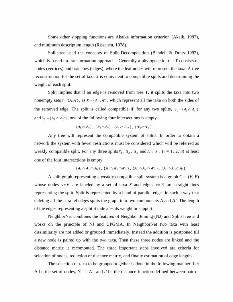
Some other stopping functions are Akaike information criterion (Akaik, 1987),

and minimum description length (Rissanen, 1978).

Splitstree used the concepts of Split Decomposition (Bandelt & Dress 1992),

which is based on transformation approach. Generally a phylogenetic tree T consists of

nodes (vertices) and branches (edges), where the leaf nodes will represent the taxa. A tree

reconstruction for the set of taxa X is equivalent to compatible splits and determining the

weight of each split.

Split implies that if an edge is removed from tree T, it splits the taxa into two

nonempty sets , as}',{ AAS = }'{ AAX ∩= , which represent all the taxa on both the sides of

the removed edge. The split is called compatible if, for any two splits, }'{ 111 AAS ∩=

and , one of the following four intersections is empty. }'{ 222 AAS ∩=

, }{ 21 AA ∩ }'{ 21 AA ∩ , }'{ 21 AA ∩ , }''{ 21 AA ∩

Any tree will represent the compatible system of splits. In order to obtain a

network the system with fewer restrictions must be considered which will be referred as

weakly compatible split. For any three splits , , and1S 2S 3S iA ∈ iS , (i = 1, 2, 3) at least

one of the four intersections is empty.

}{ 321 AAA ∩∩ , }''{ 321 AAA ∩∩ , }''{ 321 AAA ∩∩ , }''{ 321 AAA ∩∩

A split graph representing a weakly compatible split system is a graph G = (V, E)

whose nodes are labeled by a set of taxa X and edges Vv∈ Ee∈ are straight lines

representing the split. Split is represented by a band of parallel edges in such a way that

deleting all the parallel edges splits the graph into two components A and A’. The length

of the edges representing a split S indicates its weight or support.

NeighborNet combines the features of Neighbor Joining (NJ) and SplitsTree and

works on the principle of NJ and UPGMA. In NeighborNet two taxa with least

dissimilarity are not added or grouped immediately. Instead the addition is postponed till

a new node is paired up with the two taxa. Then these three nodes are linked and the

distance matrix is recomputed. The three important steps involved are criteria for

selection of nodes, reduction of distance matrix, and finally estimation of edge lengths.

The selection of taxa to be grouped together is done in the following manner. Let

A be the set of nodes, N = | A | and d be the distance function defined between pair of

nodes in A. let , , , …, be the clusters of size one or two. Then the distance for

each pair of cluster can be calculated as

1C 2C 3C nC

=),( CjCd i ||||

),(

ji

Cx Cy

CC

yxdi j

∑ ∑∈ ∈

(5)

There are two steps involved in the selection criteria are, finding the pair of

clusters that minimizes the following function,

),()2(),( jiji CCdnCCQ −= - ∑≠iK

CkCid ),( -

(6)

∑≠ jK

CkCid ),(

And the second one is to find the pair of taxa which minimizes the following function

),()2(),( yxdnyxQ −= - ∑≠iK

Ckxd )},({ - ∑≠JK

Ckyd )},({ (7)

The choice of selection criterion is determined by linearity, permutation

invariance, and consistency.

The reduction of distance is done as follows. If x and z are neighbors for y,

NeighborNet algorithm will replace x, y, and z into two new nodes u and v. the distance

from u to v is computed as:

),(),(),( aydaxdaud βα += (8)

),(),(),( azdaydavd γβ += (9)

),(),(),(),( azdaydaxdvud γβα ++= (10)

where βα , and γ are positive numbers with 1=++ γβα , and a∈A.

Theory of circular decompositions is considered for the estimation of the distance

between taxa. It can be computed as

=),( yxd ∑∈ )(

),(θ

δαSs

yxss (11)

where , Xyx ∈, )(θSS ∈ , d is circular distance and θ represents circular order. sα

is a nonnegative constant and sδ is split metric that is 0 for the pair considered in the

same part of split S, otherwise 1. The constant sα can be represented in terms of d as

given below.

)),(),(),()((21

11,,11, jijijijis xxdxxdxxdxxd −−−− −−+=δ (12)

Resources for Phylogenetic Network reconstruction

In this section we will discuss the details of Phylogenetic Network reconstruction

software such as T-REX (Makarenkov, 2001) and SplitsTree (Huson, 1998). Both are

available on the net to the researchers free of cost.

T-REX can be downloaded from http://www.info.uqam.ca/~makarenv/trex.html .

It can be used for the reconstruction of trees as well as networks. When dissimilarity

matrix is given as input to the program it either produces the tree or network according to

the command given. Different menus are provided with it such as File, View, Edit,

TREX, Data Format, Color, and Window. Data Format menu is used to specify the

format in which input is accepted by T-REX. There are seven options provided for it.

Those are: lower triangular matrix, squared matrix, upper triangular matrix, lower

triangular matrix with object names, upper triangular matrix with object names, squared

matrix with object names, and PHYLIP format (Felsentien, 1993).

TREX is an important menu, which provides the commands for different tree and

network reconstruction algorithms. The output will be saved in T-Rex file format with

extension .tre. The reticulogram constructed from given input dissimilarity matrix can be

saved as image file and this option is given in Edit menu. The output can also be saved in

famous Newick format. This program also provides an option for the reconstruction of

phylogenetic tree from dissimilarity matrix with missing data.

Steps involved in reconstruction of phylogenetic tree or network using T-REX is

given in Table1.

Table 1: Steps in T-REX for the reconstruction of phylogenetic tree or network

1. Start T-REX

2. Click the Data Format menu and select input format

3. Go to File menu and select Open (it opens a file navigator).

4. Select the input file (This file should be in the same format as defined in

step2)

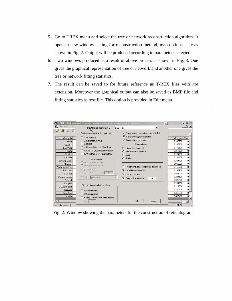
5. Go to TREX menu and select the tree or network reconstruction algorithm. It

opens a new window asking for reconstruction method, map options... etc as

shown in Fig. 2. Output will be produced according to parameters selected.

6. Two windows produced as a result of above process as shown in Fig. 3. One

gives the graphical representation of tree or network and another one gives the

tree or network fitting statistics.

7. The result can be saved to for future reference as T-REX files with .tre

extension. Moreover the graphical output can also be saved as BMP file and

fitting statistics as text file. This option is provided in Edit menu.

Fig. 2: Window showing the parameters for the construction of reticulogram

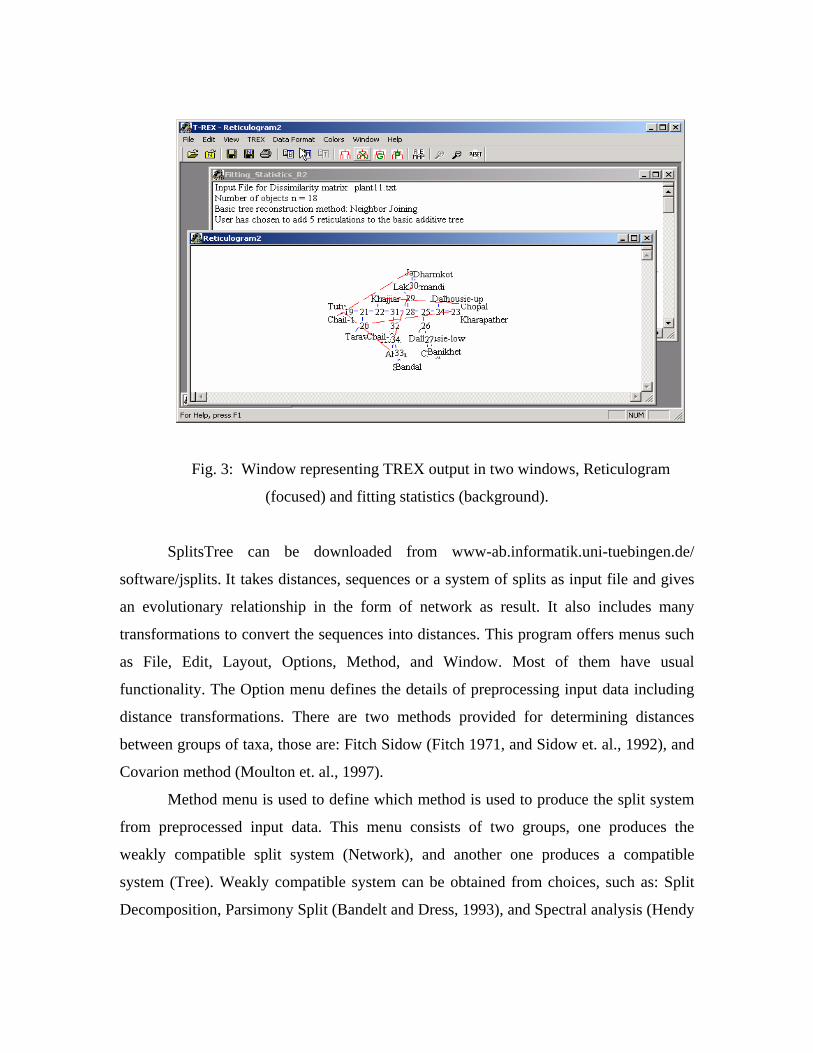
Fig. 3: Window representing TREX output in two windows, Reticulogram

(focused) and fitting statistics (background).

SplitsTree can be downloaded from www-ab.informatik.uni-tuebingen.de/

software/jsplits. It takes distances, sequences or a system of splits as input file and gives

an evolutionary relationship in the form of network as result. It also includes many

transformations to convert the sequences into distances. This program offers menus such

as File, Edit, Layout, Options, Method, and Window. Most of them have usual

functionality. The Option menu defines the details of preprocessing input data including

distance transformations. There are two methods provided for determining distances

between groups of taxa, those are: Fitch Sidow (Fitch 1971, and Sidow et. al., 1992), and

Covarion method (Moulton et. al., 1997).

Method menu is used to define which method is used to produce the split system

from preprocessed input data. This menu consists of two groups, one produces the

weakly compatible split system (Network), and another one produces a compatible

system (Tree). Weakly compatible system can be obtained from choices, such as: Split

Decomposition, Parsimony Split (Bandelt and Dress, 1993), and Spectral analysis (Hendy

and Penny; 1992). And the choices for Compatible system are: Buneman Tree (Buneman,

1971; Bandelt and Dress, 1992), P-Tree (Bandelt and Dress, 1993), and Spectral tree.

To test the statistical robustness of the spilt graph Bootstrap option is provided which

runs bootstrap sampling from given data.

Window menu contains syntax and show submenus, which are used for getting

either a syntax or current content of selected ‘nexus block’. Splitstree is based on the

nexus format (Maddison et. al. 1995) which was originally developed for PAUP

(Swafford, D., 1997), and MacClade. The output produces a file which contains different

blocks computed by SplitsTree. Steps involved in the reconstruction of phylogenetic

network using SplitsTree are given in Table 2. SplitsTree is used to for testing Split

Decomposition and NeighborNet methods.

Table 2: Steps in SplitsTree for the reconstruction of phylogenetic tree or network

1. Start SplitsTree (shown in Fig.4)

2. Go to File menu and select Open (it opens a file navigator).

3. Select the input file (This file should be in the Nexus format)

4. Select a method for reconstruction of network or tree from Method menu.

5. There are two tabs provided for result, shown if Fig. 5. The Graph tab is used

to represent the graph obtained from the input file and the Data tab gives the

tree or network fitting statistics.

6. After obtaining graph in Graph tab click on the any edge it highlights all the

edges parallel to which can be removed to represent the set of taxa which

shows conflicting relationship.

7. The result can be saved as image and text files, this option is provided in File

and Edit menus.

Fig. 4: Starting window of SplitsTree4.

Fig. 5: Selected Graph tab to view the graphical result of given Nexus input file.

Experiments and comparisons of results:

In this section we show how different algorithms provide insight into

evolutionary relationship. Here we used data sets which suits Microevolution property

and extensive polyphyly.

Experiment-1

We use the molecular data of Valeriana Jatamansi Jones, a medical plant in

western Himalaya. Random Amplification of Polymorphic DNA (RAPD) method is used

for the reliable and precise identification of the genotype. For further details (Kumar,

2003) can be referred. High level of intra-population variation exists in Valeriana

Jatamansi Jones. RAPD studies confirm that these are due to genetic origin.For present

analysis the data was transformed into a distance matrix by using the Jaccard coefficient,

shown in Table 3. This matrix is given as input to different programs.

The distance matrix shown in Table 3 served as input to the TREX. This matrix

first used to find the optimal branch length of the Jatamansi species tree using neighbor

joining method as show in Fig. 6; and second to transform the phylogenetic tree into

Reticulation Network, as shown in Fig. 7. Reticulation branches are added to the tree by

using reticulation algorithm (Makarenkov & Legendre, 2003). The distance matrix after

adding reticulations branches is shown in Table 4.

Results are analyzed based on least square loss function. The value of the least

square loss function after fitting the tree is 0.1281; it is reduced to 0.0692 after adding 14

new reticulated branches to the tree. The minimum value of the goodness-of-fit criteria

Q1, given in eq. 3, decreased from 0.0029 (without reticulation branches) to 0.0024 (with

reticulation branches). Although the phylogenetic tree well represents the major

diversities the reticulation branches were added to represent nonnegligible fraction of the

similarity that was not represented by the phylogenetic tree.

Table 3: Distance matrix of six locations calculated using Jaccard coefficients for Jatamsi Jones spices.

Location Chail-1 Taradevi Kufri Chail-2 Dalhousie-

1ow Ahala

Chail-1 0.0000

Taradevi 0.2917 0.0000

Kufri 0.2941 0.2830 0.0000

Chail-2 0.3933 0.3261 0.2857 0.0000

Dalhousie-1ow 0.3529 0.2642 0.1607 0.3673 0.0000

Ahala 0.3874 0.2696 0.2397 0.3645 0.2459 0.0000

Table 4: Distance matrix of six locations after forming Reticulation Network

Chail-1 Taradevi Kufri Chail-2 Dalhousie-

low

Taradevi 0.29172

Kufri 0.31435 0.27228

Chail-2 0.38752 0.34545 0.31796

Dalhousie-low 0.32482 0.28275 0.16070 0.32842

Alaha 0.34868 0.30662 0.23894 .32714 0.24940

Fig. 6: Phylogenetic tree (for Jatamansi Jones) associated with the Table 3 using

Neighbor Joining method

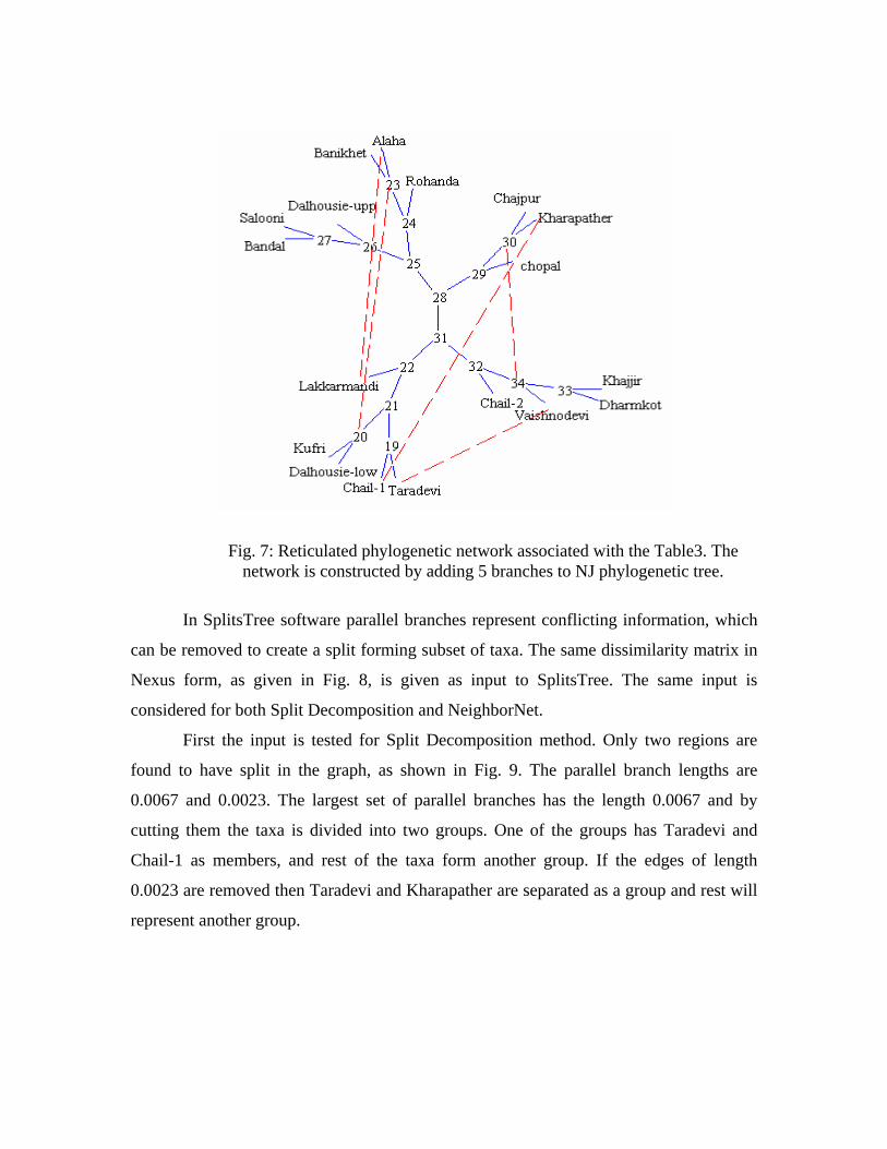
Fig. 7: Reticulated phylogenetic network associated with the Table3. The network is constructed by adding 5 branches to NJ phylogenetic tree.

In SplitsTree software parallel branches represent conflicting information, which

can be removed to create a split forming subset of taxa. The same dissimilarity matrix in

Nexus form, as given in Fig. 8, is given as input to SplitsTree. The same input is

considered for both Split Decomposition and NeighborNet.

First the input is tested for Split Decomposition method. Only two regions are

found to have split in the graph, as shown in Fig. 9. The parallel branch lengths are

0.0067 and 0.0023. The largest set of parallel branches has the length 0.0067 and by

cutting them the taxa is divided into two groups. One of the groups has Taradevi and

Chail-1 as members, and rest of the taxa form another group. If the edges of length

0.0023 are removed then Taradevi and Kharapather are separated as a group and rest will

represent another group.

------------------------------------------------------------------------------------------------------------------------------------------------ #NEXUS BEGIN taxa; DIMENSIONS ntax=6; TAXLABELS Chail-1 Taravedi Kufri Chail-2 Dalhousie-low Alalha ; END; BEGIN distances; DIMENSIONS ntax=18; FORMAT triangle=LOWER diagonal labels missing=? ; MATRIX Insert the data represented in Table 3. ; END; [distances] -----------------------------------------------------------------------------------------

Fig. 8: Sample of distance matrix in Nexus form. It will serve as input to both

Split Decomposition and NeighborNet.

Fig.9: Splits-graph associated with the distances in Fig. 8, constructed using Split Decomposition method. The circle represents two parallel edges.

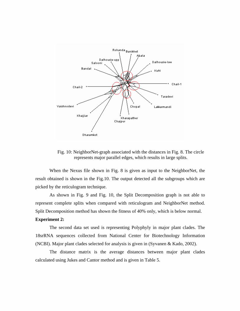
Fig. 10: NeighborNet-graph associated with the distances in Fig. 8. The circle represents major parallel edges, which results in large splits.

When the Nexus file shown in Fig. 8 is given as input to the NeighborNet, the

result obtained is shown in the Fig.10. The output detected all the subgroups which are

picked by the reticulogram technique.

As shown in Fig. 9 and Fig. 10, the Split Decomposition graph is not able to

represent complete splits when compared with reticulogram and NeighborNet method.

Split Decomposition method has shown the fitness of 40% only, which is below normal.

Experiment 2:

The second data set used is representing Polyphyly in major plant clades. The

18srRNA sequences collected from National Center for Biotechnology Information

(NCBI). Major plant clades selected for analysis is given in (Syvanen & Kado, 2002).

The distance matrix is the average distances between major plant clades

calculated using Jukes and Cantor method and is given in Table 5.

The data represented in Table 5 is given as input to TREX. Phylogenetic tree is

reconstructed using NJ method, as shown in Fig. 11, as a first step. Then the reticulogram

branches are added to the tree, as shown in Fig. 12.

The value of the least square loss function after fitting the tree is 3.024. This value

reduces to 1.701 after adding 2 new reticulated branches to the tree. The minimum value

of the goodness-of-fit criteria Q1, defined eq. 3, decreased from 0.1739 (without

reticulation branches) to 0.1630 (with reticulation branches). The distance matrix after

construction of the network is given in Table 6.

Table 5: The average distances between major plant clades calculated using Jukes, and Cantor method.

MONOCOTS 0 DICOTS 4.32 0 GYMNOSPERMS 9.62 9.44 0 BRYOPHYTES 10.09 10.07 9.97 0 FUNGI 21.50 21.52 22.52 21.52 0 CNIDARIA 22.92 22.46 23.05 20.20 19.70 0 PORIFERA 19.97 19.71 19.76 17.40 16.71 14.80 0

Table 6: Distance matrix after forming the reticulated network using NJ as tree construction method

MONOCOTS DICOTS GYMNOSPERMS BRYOPHYTES FUNGI CNIDARIA

DICOTS 4.31997 GYMNOSPERMS 9.62001 9.44001 BRYOPHYTES 10.03501 9.85501 10.24000 FUNGI 21.60000 21.42000 22.40749 20.42749 CNIDARIA 22.59925 22.41925 22.80424 20.27800 19.68301 PORIFERA 19.64325 19.46325 19.84825 17.32200 16.72702 14.79999

Fig. 11: Phylogenetic tree for major plant clades associated with the Table 5. Using Neighbor Joining method

The reticulated braches represent two subgroups as {Dicots, Monocots, and

Fungi, and another group {Bryophytes, Porifera, and Cnidaria}. The first subset

represents host- parasite relationship. The biological significance of the second group is

not known.

Fig. 12: Reticulate phylogeny associated with the Table 5. The network is constructed by

using Q1 as goodness of fit criteria to NJ phylogenetic tree.

The same data set is applied to the SplitsTree and tested using the Split

Decomposition and NeighborNet methods.

When the input is given in nexus format and Split Decomposition method is used,

the resulting graph is show in Fig. 13.

Fig. 13: Splits-graph associated with the distances in Table 5, constructed using Split

Decomposition method. The circle represents two parallel edges.

The splits found are: (1) Since the largest set of parallel braches has the length

7.10, by cutting them one separates a group containing {Cnidaria, Porifera, Fungi}, and

{Monocots, Dicots, Gymnosperms, Bryophytes}. This represents two different classes.

(2) The next split has the length 2.15 which has {Monocots, Dicots} representing their

evolutionary closeness. (3) The third split has the length 0.735 separating {Monocots,

Dicots, Gymnosperms} from rest of the taxa. All belong to the same group. (4) The

fourth split is the result of removing branches of length 0.38 separates {Bryophytes,

Cnideria, Porifera } from the rest. The graph has shown a good fitness of 96.86%. The

total number of splits found is 14.

When the same input is served to the NeighborNet method the resulting graph is

shown in Fig. 14.

Fig. 14: NeighborNet-graph associated with the distances in Table 5.

The splits found are: (1) Since the largest set of parallel braches has the

length 7.249, by cutting them one separates a group containing {Cnidaria,

Porifera, Fungi} from rest of the species. The same split is found in Split

Decomposition also. (2) The next split has the length 2.16 which has {Monocots,

Dicots} representing their evolutionary closeness. (3) The third split has the

length 0.775 that separates {Monocots, Dicots, Gymnosperms} from rest of the

taxa. All belongs to the same group. Almost all the spits are represented by both

Splits decomposition and NeighborNet are same. The two splits {Bryophytes,

Gymnosperms} and {Cnidaria, Bryophytes} are not represented by Split

Decomposition method. They are the result of removal of parallel edges of length

0.125 and 0.097 respectively. NeighborNet gives 16 splits where as Split

Decomposition gives 14 splits.

Conclusion

Both the programs, T-REX and SplitsTree, are user friendly and freely available

to researchers on almost all the platforms. We have compared the programs based on

ease of use, their application domain, and accuracy. The comparison is given in Table. 7

followed by brief explanations.

Table 7: Comparison of different phylogenetic network reconstruction Algorithms.

S

No. Property

Reticulation

Network

( T-REX)

Split

Decomposition

(SplitsTree)

NeighborNet

(SplitsTree)

1 Time

Complexity )( 4knO )( 5nO )( 3nO

2 Ease of Use Easy Moderate Moderate

3 Accuracy High Low High

4 Phylogenetic

Tree

Dependency

Yes No No

5 No. of Useful

Splits Moderate Less More

6 Application

Domain

microevolution,

homoplasy

viral data, plant

hybridization

gene transfer,

branching in

Eukaryotes

As given in Table 7, the time complexity for T-Rex Algorithm is , where k

is number of reticulated branches, and n is number of species.

)( 4knO

Ease of use property is measured on the basis of T-REX and SplitsTree software.

SplitsTree accepts the input in nexus format, which should be known priory to the user,

where as T-REX accepts the input in very simple format, which is clear from Fig. 3 and

Table 3 respectively.

In application domain we mentioned where the Algorithms are used by this time.

SplitsTree has been used to analyze viral data, plant hybridization and evolution of

manuscripts. T-REX has been used for micro evolution, homolpalsy, hybridization and

lateral gene transfer.

T-REX computes Reticulation Network by first computing a phylogeny and

subsequently a network by adding branches (represented as dashed edges) which

minimizes certain least square loss function. This restriction could be time consuming

and cause problem if the data is not tree like.

Split Decomposition is quite conservative. It only represents splits of taxa with positive

isolation index. Many splits with negative isolation index are removed. But they may

represent some conflicting information.

NeighborNet method tends to produce more resolved network than Splits

decomposition. T-Rex is most accurate, but time consuming. However, NeighborNet is

most efficient (time) and accurate enough for our data set.

Acknowledgements

We are grateful to Amit Kumar, Saurabh Agarwal and Osman Basha for helping

in analyzing the results.

References Akaike, H., (1987), Factor analysis and AIC, Psychometrika, 52, 317–332. Bandelt, H.-J., and Dress, A.W.M., (1992), Split Decomposition: A new and useful approach to phylogenetic analysis of distance data. Molecular Phylogenetics and Evolution 1, 242–252. Bandelt, H.-J., and Dress, A.W.M., (1993), A relational approach to Split Decomposition. In Opitz, O., Lsusen, B. and Kalar, R.,(eds), information and classification, Springer, Berlin, pp 123-131. Brown, T. A., and Brown, K .A, (1994), Using molecular biology to explore the past, Bioassays 16: 719-726. Bryant, D., and Moulton, V., (2002), NeighborNet: An agglomerative method for the construction of planar phylogenetic networks, in R. Guigo, D. Gusfield, eds., 2nd Workshop on Algorithms in Bioinformatics, 375–391, LNCS 2452, Springer. Buneman, P., (1971), The recovery of the trees from measures of dissimilarity, In mathematics and archeological and historical sciences, Edinburgh Univ. Press, pp 387-395. Felsenstein, J., (1982), Numerical methods for inferring evolutionary trees, Quar. Rev. Biol. vol. 57(1), pp 379–404. Felsenstein, J., (1993), PHYLIP: Phylogeny Inference Package, version 3.5c, University of Washington.

Fitch,W. M., and Margoliash, E., (1967), A non-sequential method for constructing trees and hierarchical classifications, Journal of Molecular Evolution, 18, 30-37. Fitch, W., (1971), Towards defining the course of evolution: minimum change for a specific tree topology, Syst. Zool, 20, 406-416. Hendy, M. D., and Penny, D., (1992), Spectral analysis of phylogenetic data, J. Classfic., 10, 5-24. Huson. D. H., (1998), SplitsTree: A program for analyzing and visualizing evolutionary data. Bioinformatics 141, 68-73. Kumar, A., (2003), Characterization of Indian Valerian (Valeriana jatamansi Jones) Germplasm in Himachal Pradesh using molecular markers, Masters Thesis, College of Horticulture, Dr. Yashwanth singh parmar Univ., Nauni, Solan, Himachal Pradesh, India. Lapointe, F.-J., and Landry, P.-A., (1997), Estimation of Missing Distances in Path-Length Matrices: Problems and Solutions. Pp. 209-224, in Mathematical hierarchies and Biology (B. Mirkin, F.R. McMorris, F. Roberts, A. Rzhetsky, eds.), DIMACS Series in Discrete Mathematics and Theoretical Computer Science, Amer. Math. Soc., Providence, RI, 1997, 209-224. Legendre, P., (2000), Biological applications of reticulation analysis, Journal of Classification, 17, 153-157. Legendre, P., and Makarenkov, V., (2002), Reconstruction of Biogeographic and Evolutionary Networks Using Reticulograms. Systematic Biology 51, 199-216. Levasseur, C., Landry, P. A. and Lapointe, (2000), Estimating Trees from Incomplete Distance Matrices: a Comparison of Two Methods, Data analysis, Classification and Related Methods (H. A.L. Kiers, J.-P. Rasson, P. J.F. Groenen, M. Schader, eds), 149-154. Rissanen, J., (1978), Modeling by shortest data description, Automatica 14, 465–471. Makarenkov, V., and Leclerc B., (2000), Comparison of additive trees using circular orders, Journal of Computational Biology, 7, 731-744. Makarenkov, V. (2001), T-Rex: reconstructing and visualizing phylogenetic trees and Reticulation Networks. Bioinformatics 17, 664-668. Makarenkov, V. and Legendre, P. (2003), From a phylogenetic tree to a reticulated network, submitted to Journal of Computational Biology.

Syvanen, M., and Kado, C. L., (2002), Horizontal Gene Transfer, Second Edition,Academic Press, NY. Moulton, V., Steel, M. A. and Tuffely, C., (1997), Dissimilarity maps and substitution models: some new results, Proceedings of the DIMACS workshop on mathematical hierarchies and biology, American Mathematical Society, in press. Sidow, A., Nguyen, T. and Speed, T. P., (1992), Estimating the farction invariable codons with a capture-recapture method. J.Mol. Evol., 35, 253-260 Sokal, R. R., and Michener, C.D., 1958, A statistical method for evaluating systematic relationships, Univ. Kansas Sci. Bull., 28, 1409-1438. Sonea, S., and Panisset, M., (1976), Pour une nouvelle bacteriologie. Revue Canadienne de Biologie, 35, 103-167. Swafford, D., (1997), PAUP: Phylogenetic Analysis Using Parsimony (and Other Methods), version 4.0 (test version), Sinauer Associates, Inc., Sunderland, MA. Swafford, D. L., and Olsen, G. L., (1996), Phylogeny reconstruction, 407-514. In D. M. Hill (eds), Molecular Systematics. Sinauer. Yushmanov, S.V. (1984), Construction of a tree with p leaves from 2p-3 elements of its distance matrix (Russian), Matematicheskie Zametki 35, 877-887.