L: : _i

M illim eter-w ave Spectra

of the Jovian Planets

By

Joanna Joiner

Paul G. Steffes, Principal Investigator

School of Electrical Engineering

Georgia Institute of Technology

Atlanta, GA 30332-0250

.(404) 894-3128

August, 1991

k

Technical Report No. 1991-1

Prepared under NASA grant NAGW-533

Unclos343

i

https://ntrs.nasa.gov/search.jsp?R=19910021739 2018-09-08T14:03:46+00:00Z

11--

PRFCEDi_G P.AGE _LAt_;K NOT RLMED

===

]]]

Acknowledgments

I am indebted to my advisor, Paul G. Steffes, for his guidance, optimism, con-

fidence, and patience. I thank him for his assistance during this research and

for preparing me for life beyond graduate school. I thank the following fac-

ulty committee members for their time and careful examination of the document:

A. J. Gasiewski (reader), G. S. Smith (reader), J. A. Buck (chairman of the qual-

ifying and proposal committees), and C. G. Justus.

I thank D. P. Campbell and S. Halpbern of the Georgia Tech Research In-

stitute (GTRI) and T. E. Brewer (Georgia Tech) for their generous assistance

with the laboratory equipment and for providing illuminating discussions. I also

thank J. J. Gallagher (GTRI) whose selflessness and courage is an example for

all. I thank the staff of the Caltech Submillimeter Observatory (CSO), especially

T. D. Groesbeck and A. E. Schincke], for their assistance with the hardware and

data analysis at the CSO. I also thank T. R. Spilker (Stanford), I. dePater (Berke-

ley), V. N. Romani (SSAI, NASA-Goddard), K. S. Noll (NRC, NASA-Marshall),

B. Bezard, and E. LeUouch (Observatoire de Paris-Meudon) for illuminating dis-

cussions and helpful suggestions.

Finally, I thank the following family and friends for their constant support and

encouragement and for putting up with me during diffcult times: Noel and Selma

Wang, J. Robert and Valerie Joiner, Jennifer and Gilbert Lawson, Mary Frances

Joiner, Bess Fleckman, Elsie Wang, Cliff Wang, Keith Noll, Michael Wileman, Jon

Jenkins, Tony Fahd, Cindy Stokes, Lori Cabena, and Lynne Patterson.

This work was supported by the Planetary Atmospheres Program of the

Solar System Exploration Division (Office of Space Science and Applications) of

the National Aeronautics and Space Administration under grant NAGW-533 and

by the Georgia Tech Space Grant Consortium.

iv

Contents

I INTRODUCTION 1

I.I Background and Motivation ...................... 1

1.2 Organization .............................. 4

2 Laboratory Measurements of Ammonia (NHs) and Hydrogen Sul-

fide (H2S) Absorption Under Simulated Jovian Conditions 6

2.1 Propagation in a Lossy Dielectric ................... 6

2.2 Measurements of Ammonia (NHs) Opacity at Ka-band and W-band 8

2.2.1 Laboratory Configuration ................... 9

2.2.2 Experimental Approach .................... 16

2.2.3 Experimental Uncertainties .................. 20

2.2.4 Theoretical Characterization of Ammonia Absorption . . . 23

2.2.5 Experimental Results and Interpretation ........... 28

2.3 Measurement of Hydrogen Sulfide (H_S) Opacity at G-band .... 35

2.3.1 35

2.3.2 38

2.3.3 38

2.3.4 39

Laboratory Configuration and Procedure ..........

Experimental Uncertainties ..................

Theoretical Characterization of H2S Absorption .......

Experimental Results .....................

3 Modeling of the Jovian Atmospheres 41

3.1 Thermochemica] Modeling ....................... 41

3.2 Theory of Radiative Transfer ..................... 45

3.2.1 The Radiative Transfer Equation ............... 45

3.2.2 Disk-averaged Brightness ................... 47

V

3.3 Parameters of the Radiative Transfer Model (RTM)

3.3.1

3.3.2

3.3.3

Temperature-Pressure Profile .................

Opacity ............. ................

Vertical Distributions of Opacity Sources ..........

3.4 Modeling Results ............................

3.4.1

3.4.2

3.4.3

3.4.4

3.,5

The radio spectrum of Jupiter ................

The radio spectrum of Saturn .................

The radio spectrum of Uranus ................

The radio spectrum of Neptune ................

Conclusions and Comparisons .....................

54

54

56

67

67

68

81

83

87

90

4 Dual Wavelength Observation of Jupiter at 1.4 mm 03

4.1 Sensitivity Calculation ......................... 95

4.2 Instrumentation and Procedu_re . , . ....... , . ..... . . . 97

4.3 Calibration ............................... 105

4.4 Atmospheric Conditions ........................ 113

4.5 Data Analysis ................................ 116

4.6 Observational Results ......................... 124

5 Summary and Conclusion 120

5.1 Uniqueness of Work ................. , ......... 129

5.2 Suggestions for Future Research .................... 130

vi

List of Figures

2.1

2.2

2.3

2.4

2.5

2.6

2.7

2.8

2.9

2.10

2.11

2.12

3.7

3.8

3.9

Block diagram of the Ka-band atmospheric simulator ........ 10

Block diagram of the W-band atmospheric simulator ........ 11

Sketch of the Ka-band Fabry-Perot resonator ............ 13

Sketch of the W-band Fabry-Perot resonator ............ 14

Sketch of the ammonia (NHs) molecule ................ 24

Theoretically computed ammonia absorption ............ 27

Measured and theoretical Ka-band absorption from gaseous NHs 31

Measured and theoretical W-band NHs absorption at 2 atm .... 32

Measured and theoretical NHs absorption at 8 atm ......... 33

Measured and theoretical W-band NHs absorption at 1 atm .... 34

Block diagram a transmission cell for measuring H=S absorption.. 36

Measured and theoretical G-Band absorption from gaseous H=S . . 40

3.1 Sketch of the zenith angle of a planet ................. 46

3.2 Grid of Jupiter .............................. 49

3.3 Geometry of an oblate spheroid .................... 50

3.4 The 1 bar surfaces of Jupiter and Saturn ............... 52

3.5 Computed H2S absorption ....................... 58

3.6 Computed pressure-induced absorption from H=-H2, H2-He, and H=-

CH4 ............. • ..................... 60

Computed H20 absorption ....................... 61

Temperature-pressure profiles of the Jovian planets ......... 69

Vertical distributions and cloud bulk densities in Jupiter's atmosphere. 73

vii

3.10

3.11

3.12

3.13

3.14

3.15

3.16

3.17

3.18

3.19

4.8

4.9

4.10

4.11

4.12

4.13

Jupiter's observed and computed spectrum using NH3, H20, and

pressure-induced opacity only. ..................... 75

Jupiter's observed and computed spectrum with NHs, H2S, PHs,

and H_O opacity. ............................ 76

Weighting functions at 1 ram, 1.4 ram, 1 cm, and 10 cm for Jupiter. 78

Jupiter's observed and computed spectrum with cloud opacity. . . 82

Vertical distributions of NHs and cloud bulk densities in Saturn's

atmosphere ............................... 84

Saturn's observed and computed spectrum .............. 85

Weighting functions at 1 ram, 1 era, and 10 cm for Saturn ..... 86

The observed and computed spectrum of Uranus ........... 88

Weighting functions for Uranus at 1 ram, 3 ram, 1.3 cm, 10 cm... 89

The observed and computed spectrum of Neptune .......... 91

4.1 Block diagram of the Caltech Submillimeter Observatory (CSO). 98

4.2 Block diagram of the CSO 230 GHz receiver ............. 99

4.3 Effect of H2S absorption at 216 GHz and frequencies at which we

observed Jupiter with the double side band (DSB) CSO receiver.. 102

4.4 Plot of air masses of Jupiter and Mars on 26 November ....... 104

4.5 Typical observed spectrum of Mars .................. 107

4.6 Map of Jupiter at 230 GHz ....................... 110

4.7 Equatorial cut through the beam map of Jupiter and the computed

brightness temperature ......................... 111

Plot of the beam shape of the CSO at 230 GHz ........... 112

Plot of • as a function of hour for 25 November ........... 114

Plot of r as a function of hour for 26 November ........... 115

Average of Jupiter scans at 215.3 GHz for 25 November ....... 125

Average of Orion scans at 215.3 GHz for 26 November ........ 126

Observed and theoretical spectrum of Jupiter near 216 GHz .... 127

mw_

Vlll

List of Tables

2.1 Measured and theoretical values of NHs absorption ......... 29

3.1 Specific heat of atmospheric constituents ............... 56

3.2 Model parameters ........................... 70

3.3 List of reliable millimeter observations of Jupiter .......... 71

3.4 Potential cloud reflectivities, transmisivities, and resulting change

in Jupiter's brightness temperature due to clouds .......... 80

3.5 Magnitude of absorption coefficients (in cm -1) at 1 bar, 1 mm... 92

4.1 Listing of observations (UT) 25 November 1990 at 216 GHz ..... 117

4.2 Listing of observations (UT) 26 November 1990 at 230 GHz ..... 118

4.3 Listing of observations (UT) 26 November 1990 at 216 GHz ..... 119

4.4 Observed antenna temperatures .................... 121

4.5 Observational data used to computed Jupiter's brightness temper-

ature ................................... 122

4.6 Observed Jovian brightness temperatures near 1.4 mm ....... 123

Summary

The millimeter-wave portion of the electromagnetic spectrum is critical for

understanding the subcloud atmospheric structure of the Jovian planets (Jupiter,

Saturn, Uranus, and Neptune). This research utilizes a combination of laboratory

measurements, computer modeling, and radio astronomical observation in order to

obtain a better understanding of the millimeter-wave spectra of the Jovian planets.

The pressure-broadened absorption from gaseous ammonia (NHs) and hydrogen

sulfide (H_S) has been measured in the laboratory under simulated conditions for

the Jovian atmospheres. We have developed new formalisms for computing the

absorptivity of gaseous NHs and H_S based on our laboratory measurements. We

have developed a radiative transfer and thermochemical model to predict the abun-

dance and distribution of absorbing constituents in the Jovian atmospheres. We

use the model to compute the millimeter-wave emission from the Jovian planets.

The model utilizes the results of the laboratory measurements and is also used

to evaluate other possible candidates for millimeter-wave absorption in the Jovian

atmospheres. Finally, we have observed Jupiter near 1.4 mm using the Caltech

SubmUlimeter Observatory (CSO) in an attempt to detect gaseous hydrogen sul-

fide. Sulfur compounds have been identified on Io, one of Jupiter's moons, but

they have never been detected on any of the Jovian planets. Although we were

not able to detect hydrogen sulfide, we were able to make a good observation of

Jupiter's brightness temperature at this wavelength using Mars as the calibration

standard. This research ultimately adds to the understanding of the composition

and cloud structure of the Jovian planets and provides clues to the origin and

evolution of the planets and solar system.

CHAPTER 1

INTRODUCTION

Section 1.1 lays the foundation for this work as it relates to the study of the Jovian

atmospheres. The organization of the document follows in Section 1.2.

1.1 Background and Motivation|

The Jovian planets (Jupiter, Saturn, Uranus, and Neptune) are the most massive

planetary bodies in our solar system. They are also known as the gaseous giant

planets because a significant fraction of their mass is contained within their atmo-

spheres. Atmospheric features such as the great red spot on Jupiter were observed

as early as the 17th century. However, little was known about the composition

of the Jovian atmospheres until this century. Advances in instrumentation over

the past few decades have allowed scientists to compile much new information

about the atmospheric structure and composition of the Jovian planets. The use

of instruments aboard spacecraft has enhanced this new wealth of information.

The abundances of elements observed in the atmospheres of the four Jovian

planets provides one of the biggest clues to the origin and evolution of the planets.

The Jovian planets have retained much of their original atmospheres, unlike their

inner solar system counterparts (Venus, Earth, and Mars). The most abundant

elements in the Jovian atmospheres (and the solar system) are hydrogen and he-

lium. Small abundances of other elements are found to exist primarily in reduced

forms. The heavier volatiles such as CH4, NHs, and H2S appear to be enriched

2

(relative to the sun) in the atmospheresof the giant planets (see, e.g., de Pater

eta/., 1989 and Grossman, 1990). The enrichment of heavier elements favors the

core-instability model (see, e.y., Pollack and Bodenheimer, 1989) in which the

core of the giant planets is formed first by solid accretion. When a critical mass

is reached, the planet begins to rapidly accrete gas from the surrounding solar

nebula.

Only six minor elements have been positive]y detected on the giant planets.

These elements, carbon, oxygen, nitrogen, phosphorous, germanium, and arsenic,

form a cluster in the periodic table. Sulfur remains mysteriously absent from this

list. The formation of clouds may deplete sulfur (in the form of gaseous H2S) in the

upper atmospheres of the Jovian planets, making it difficult to detect with con-

ventiona] methods. Ground and space based radio observations and experiments

provide one of best means to extract information about the presence and abun-

dance of absorbing constituents, including H2S, below the optically thick clouds.

One goal of this research is to use the millimeter-wave spectrum to search for

gaseous H2S on Jupiter.

Radio occultation is an example of a space-based experiment which can pro-

vide information about the subcloud regions of the giant planets. During an oc-

cultation, a spacecraft travels behind a planet and transmits a stable CW signal

through the atmosphere of the planet. This signal is refracted and attenuated as

it passes through the atmosphere of the planet. The resulting signal is received on

the earth. Information about the planetary atmosphere can be inferred from the

precise measurement of the signal's frequency shift and attenuation. For example,

the Voyager spacecraft have been used in radio occultation experiments to retrieve

temperature-pressure profiles for all four of the Jovian planets (see, e.g., Lindal,

eta/., 1981). These experiments typically take place at S and X Band (between

2.3 and 8.4 GHz). Radio occultatlous are limltedin that a single occultation can

provide information only at one localized area of the planet. The data from only

one location may not be representativeof the conditions elsewhereon the planet.

The expected arrival of the Galileo spacecraft st Jupiter in 1995 and the

Cassini mission to Saturn in the next century will provide additional clues to the

composition of the two closest Jovian planets. These spacecraft will drop probes

into the atmosphere of the planets. Mass spectrometers will identify gases within

the atmosphere. Again, this type of in-aitu observation is limited in that a single

probe gives information for only one location on the planet.

Ground-based radio astronomy has x distinct advantage over these space-

based experiments in that the entire planet is observable with a single radio tele-

scope or an array of telescopes. Many observations of the emission from the giant

planets have been made with radio telescopes at wavelengths from I mm to several

meters. However, the interpretation of the observations is still in the initial stages.

Laboratory studies of potential absorbers are needed in order to correctly inter-

pret the measured emission from the planets. The dearth of laboratory absorption

measurements under planetary conditions has hampered the interpretation of the

Jovian millimeter-wave spectra in the past. Another goal of this research is to be-

gin a program of laboratory measurements so that the available observations can

be correctly interpreted. The millimeter-wave region of the spectrum will then be

an important piece of the puzzle which theorists use to piece together the origin

and evolution of the planets.

Another difficulty in interpreting millimeter observations of the giant planets

is the large uncertainty in the absolute flux calibration. Accurate calibration of the

millimeter wavelength planetary observations is critical if meaningful comparisons

are to be made between different observations and between the observations and

radiative transfer models. Mars is the moet frequently used calibrator at these

wavelengths. However, the uncertainty in the estimated flux from Mars is reported

to be appraximately 10_ (Griffin et a/., 1986). Before the millimeter-wave spectra

of the Jovian planets are fully understood, better calibration techniques will be

4

needed.

A long standing discrepancy between modeled and observed brightness tem-

peratures of Jupiter at millimeter wavelengths (see, e.g., de Pater and Massie,

1985) provided the initial motivation for this work. One of the largest uncer-

tainties in modeling the mUlimeter-wave emission from the giant planets is the

absorption coefficient of gaseous ammonia (NHs). This gas is by far the strongest

millimeter wave opacity source on Jupiter. This work began with laboratory mea-

surements of the millimeter-wave absorption from gaseous NHs under simulated

Jovian conditions. The experiments were conducted at two frequency bands where

a number of radio astronomical observations have been made. The results of the

experiments were incorporated into a radiative transfer model which predicts the

radio emission from the Jovian planets. The results of the radiative transfer mod-

eling provided the motivation for a millimeter-wave observation of 2upiter in an

attempt to detect gaseous hydrogen sulfide (H2S). A laboratory measurement of

the pressure-broadening effects of hydrogen and helium onhydrogen sulfide was

designed in order to correctly interpret the observation.

This work contributes new experimental, theoretical, and observational re-

suits which lead to a better understanding of the millimeter-wave spectra of the

2ovian planets. Millimeter-wave instrumentation for planetary spectroscopy is still

in an evolutionary state and will continue to provide new and improved planetary

observations in the future. The results of the laboratory measurements presented

in this work will help to interpret past, present, and future observations of the

giant planets. It is hoped that this work will stimulate future research in this

area.

1.2 Organization

The scope of this research may be conveniently divided into three areas:

5

. Laboratory measurements of the millimeter-wave absorption from gaseous

ammonia (NHs) and hydrogen sulfide (H2S) in a simulated Jovian atmo-

sphere

2. Radiative transfer and thermochemical modeling of the Jovian atmospheres

3. Dual-wavelength radio astronomical observation of Jupiter at 1.4 mm

Chapters 2, 3, and 4 discuss each of these areas, respectively.

Chapter 2 describes the laboratory configuration, experimental methodology,

and results of millimeter-wave absorptivity measurements of gaseous ammonia

(NH3) and gaseous hydrogen sulfide (H_S) under simulated Jovian conditions.

The results are compared with various theories used to predict the millimeter-

wave absorptivity of these gases.

The theory and application of a radiative transfer and thermochemical model

are described in Chapter 3. We use a forward approach to model the emission from

each of the giant planets. In a forward approach, the parameters of the radiative

transfer model (i.e., the abundances and distributions of absorbing constituents

in the planetary atmospheres) are adjusted in order to obtain a good fit to the

observed millimeter-wave spectra. The radiative transfer model utilizes the results

of the laboratory measurements described in Chapter 2. We also develop new

formalisms to compute the opacity from other sources in the Jovian atmospheres

(e.g., pressure-induced absorption and water vapor absorption).

Chapter 4 describes the approach, analysis, and results of a dual-wavelength

radio astronomical observation of Jupiter at 1.4 mm. Relevant aspects of the

instrumentation and calibration are described in detail.

A summary of the major conclusions and contributions of this work is pre-

sented in Chapter 5. In addition, this chapter provides several suggestions for

future research.

6

CHAPTER 2

Laboratory Measurements of Ammonia

(NH3) and Hydrogen Sulfide (H2S)

Absorption Under Simulated Jovian

Conditions

One of the outstanding problems in the millimeter spectroscopy of planets has been

and continues to be the lack of adequate laboratory measurements of line shapes

and widths of gases at relevant pressures and temperatures and with appropriate

broadening agents. This chapter describes the laboratory apparatus, procedure,

and results of gaseous ammonia (NHs) and hydrogen sulfide (H2S) absorptivity

measurements under simulated Jovian conditions. The implications of the results

presented in this chapter will be explored in Chapter 3.

2.1 Propagation in a Lossy Dielectric

The electric and magnetic fields of forward traveling waves in a lossy dielectric

assume the form

E(z) = Eoe-'fe -yp, (2.1)

and

H(,) = Hoe-"e-_p', (2.2)

7

respectively, where a and/3 are known as the propagation constants; a is called

the attenuation constant or absorption coefficient, and/3 is called the phase con-

stant. The propagation constants are related to the related to the permittivity e

and permeability/z of the medium through which the wave travels as well as the

frequency w. In general, the permittivity of gases is complex and assumes the form

t -- e'-- its. (2.3)

The permeability _ is approximately equal to the permeability of free space _o.

The propagation constants for gases in general are

(2.4)

and

respectively. Their ratio is

o |[!+(s)']'"= _ {*'-'_21_12/3 [l+k,,/ J +1

(2.5)

(2.6)

The loss tangent of a gaseous medium is defined as

tan_ = E" (2.7)

and the quality factor in a gaseous medium (Qe) is

Q' = tant = 7" (2.8)

For a low-loss gas, the loss tangent is much less than unity. In this case,

Equation 2.6 reduces to

The phase constant/3 is

= 2-_" (2.9)

2_r

/3- -_-, (2.10)

8

so that the absorption coe_icient can be written as

(2.11)

2.2 Measurements of Ammonia (NH3) Opacity

at Ka-band and W-band

The absorption from gaseous ammonia strongly affects the millimeter-wave spec-

tra of the giant planets. Ammonia is by far the largest millimeter-wave opacity

source on Jupiter and Saturn. The opacity from gaseous ammonia must be known

accurately before the potential effects of other absorbing constituents can be as-

sessed.

Steifes and Jenkins (1987) have measured the absorption from gaseous am-

monia between 1.38 and 18.5 cm (1.6 to 22 GHz). They have shown that to within

experimental accuracy the absorptivity of gaseous NHs is correctly expressed by

the modified Ben-Reuven line shape as discussed by Berge and Gulkis (1976).

However, no laboratory absorption measurements have been made under simu-

lated Jovian conditions at frequencies above 22 GHz (wavelengths less than 1.35

cm). Therefore, it is not known whether the use of the modified Ben-Reuven line

shape is appropriate for computing gaseous ammonia opacity at frequencies above

22 GHz.

In order to test the Ben-Reuven and other line shapes, we have measured the

opacity of gaseous ammonia (NHs) under simulated Jovian conditions at several

millimeter wavelengths. We conducted one set of experiments at several Ka-band

frequencies between 32-40 GHz (7.5-9.38 ram). We conducted a second set of

experiments at a frequency of 94 GHz or 3.2 mm (W-band). We conducted the

experiments using mixing ratios of hydrogen, helium, and NHs which are similar to

those found on Jupiter. Jupiter's atmosphere is approximately 90% H2, 10% He,

and 0.025% or 250 parts per million (ppm) NHs. In order to measure absorption,

9

we need a higher NHs mixing ratio than that found on the Jovian planets. We

used a mixture consisting of 88.34% hydrogen (H2), 9.81% helium (He), and 1.85%

ammonia (NHs) for the Ka-band experiment. This corresponds to an NHs partial

pressure of 28 tort within a total gas mixture pressure of 1560 tort (2 atm). The

temperatures and pressures used in the experiments closely resemble those found

in Jupiter's atmosphere at altitudes which emit Ka-band radiation. We conducted

the experiments at a pressure of 2 atm and at a temperature of 203 K. A higher

mixing ratio of NHs is needed in order to measure W-band absorption, because

W-band ammonia opacity is significantly less than that at Ka-band. We used a

mixture of 85.56_ H2, 9.37% He, and 5.07% NHs for the W-band experiment. The

W-band experiment took place at a temperature of 210 K in order to avoid conden-

sation. The pressures of the W-band experiments ranged from 1 to 2 atm. These

experiments represent the first time that the opacity of gaseous _onia has been

measured under simulated conditions for the Jovian atmospheres at wavelengths

less than 1 cm.

2.2.1 Laboratory Configuration

Figures 2.1 and 2.2 show block diagrams of the Ka-band and W-band atmospheric

simulators. The components of the simulators may be grouped into the three sub-

systems: an electrical subsystem, a gaseous pressure subsystem, and a temperature

chamber (an ultra-low temperature freezer).

The electrical subsystem of a general millimeter-wave atmospheric simulator

is composed of an absorption cell, a millimeter-wave source, and a millimeter-

wave receiver. For the Ka-band experiment, the electrical subsystem is a Ka-

band Fabry-Perot resonator, a millimeter-wave, swept oscillator (Hewlett-Packard

8690B), and a high resolution spectrum analyzer (Tektronix 7L18). The spectrum

analyzer provides the local oscillator (LO) for an external harmonic mixer. The

W-band electrical system is similar to the Ka-band system. The source is a power

10

H2

Vm

I- v I I

I

Rumnator

-1

Figure 2.1: Block diagram of the Ka-band atmospheric simulator

ORiGi_'_AL PAGE IS

OF POOR QUALITY

11

W-BandM,limeter-wave

SweepOscillator

94 GHz (3.2 ram)

H2 _:_ RegulatorSource

Source Regu_tor

Custom _[Mixture Regulator

F-

I I I] Power M_owav.Supply Frequency

I co..t_

I aaJward I locked' W.v. I I t tPhase

_- spoct_n

I__ _T_J_I 1.5 GHzIsolator "_ 94" GHz

MixerVacuum Pressure

Gauge Gauge _ _

Vacuum

Pump

ResonatorI

_Temperature

_Vl_m_ [ Chamber

Figure 2.2: Block diagram of the W-band atmospheric simulator

12

supply (Micro-Now 70SB)and backward-wave oscillator (BWO) tube (Micro-Now

Model 728 RWO 110) which act together as a millimeter-wave, swept oscillator.

The local oscillator (LO) for the harmonic mixer is a microwave source, phased

locked to a microwave frequency counter. The mixer combines the tenth harmonic

of the LO with the outgoing signal from the resonator. This produces an inter-

mediate frequency (IF) of approximately 1.5 GHz. The high resolution spectrum

analyzer displays the IF signal.

The Ka-band Fabry-Perot resonator (shown in Figure 2.3) consists of two

gold plated mirrors contained in a T-shaped glass pipe. The mirrors are sepa-

rated by a distance of approximately 20 cm. The resonator is a semi-confocal

configuration in that one mirror is fiat and the other is spherical. The resonant

frequency can be changed by turning a micrometer connected to the spherical mir-

ror which adjusts the mirror spacing. The quality factor (Qc) of this resonator

is approximately 8000. The W-band Fabry-Perot resonator shown in Figure 2.4

is also semi-confocal. This resonator differs from the Ka-band resonator in that

the fiat mirror has a much smaller radius (5 cm) than the spherical mirror (11.5

cm). The two mirrors are separated by a distance of approximately 14 cm. This

type of configuration yields superior focusing which results in a high quality factor

(Qc) of the resonator (approximately 25,000). The W-band resonator is contained

in a cross shaped glass pipe with the curved mirror resting on two fixed support

arms. The fixed arms can be adjusted in order to change the distance between

the mirrors without disturbing the sensitive alignment. Any adjustments to the

mirror spacing and alignment takes place before the resonator is placed in the

temperature chamber.

The mirrors were originally constructed of aluminum with a thin layer of gold

sputtered on the surface of the mirrors in order to minimize resistive losses. After

several sets of experiments, we noted a degradation in the quality factor (Qc) of

the resonator. An inspection of the resonator revealed that ammonia had reacted

13

_'ro_' _

/_m_ Ptsto -_

/_te tr/ot

Figure 2.3: Sketch of the Ka-band Fabry-Perot resonator

14

SuPj_rns_rt

Figure 2.4: Sketch of the W-band Fabry-Perot resonator

15

with the aluminum. This reaction caused the gold to peel off the surface of the

mirrors. In order to correctthisproblem, the mirrors were refabricatedusing brass

and sputtered with gold.

The Fabry-Perot resonator operates as a band pass filterat each resonance.

The millhneter-wave sweep oscillatoris adjusted for each resonance so that it

sweeps through the entirefrequency range affectedby that resonance. We measure

the band width of each resonance with the high resolution spectrum analyzer.

Electromagnetic energy iscoupled both to and from the resonator through twin

iriseslocated on the flatmirror. The irisesare attached to two sections of rigid

waveguide which are sealed with rectangular pieces of mica held in place by a

mixture of rosin and beeswax. Flexible Ka-band waveguide and rigid W-band

waveguide connect the resonator (insidethe temperature chamber) to the sweep

oscillatorand mixer (outside the temperature chamber) through a small hole in

the temperature chamber.

The gaseous pressure subsystem consistsof the cylinders containlng the var-

ious gases used in the experiments (H2, He, NHs, and custom mixtures), two oii

diffusionvacuum pumps, a thermocouple vacuum gauge tube (0-27 torr),a posi-

tive pressure gauge (0-100 PSIG), and a glass pipe which contains the resonator.

Each of the open ends of the pipe issealed with an O-ring sandwiched between the

glass lip and a fiatbrass or aluminum plate which isbolted to an inner flange. A

network of 3/8" stainlesssteeltubhug and valves connects the components of the

pressure subsystem, so that each component may be isolatedfrom the system as

necessary (seeFigures 2.1 and 2.2). When properly secured, the system iscapable

of containing two atmospheres of pressure without detectable leakage.

Precautions have been taken to allow for the proper ventilationof the hydro-

gen and ammonia gas so that the experiment can take place indoors. We use a

flammable gas detector to detect any leaks during the experiment. All gases are

released outdoors through a vent pipe where they are safelydiluted by air.

16

2.2.2 Experimental Approach

The Fabry-Perot resonator provides the sensitivity needed to measure the millimeter-

wave aborptivity of gaseous NHs. For a Fabry-Perot resonator or interferometer,

the quality factor of a resonance (loaded or unloaded) is expressed by

2_rd

Qc _ "_', (2.12)

(see, e.g., Valkenburg and Derr, 1966) where _ is the wavelength of the resonance, d

is the mirror spacing, and ic represents the total loss of the resonator per reflection.

The total loss includes coupling loss, mirror loss, diffraction loss, and any loss

due to absorbing material in the resonator. The effective path length (EPL) for

electromagnetic energy in the resonator is the ratio of d to ic or

EPL - 2_r (2.13)

The addition of a Iossy material in the resonator increases ic which results in a

reduced path length. The effective path length (unloaded) for both experiments

was approximately 10 m.

The quality factor (Qc) of a resonance is equal to the ratio of the energy

stored in the resonator to the energy lost per radian. The quality factor of a

cavity resonance in general is

/cQc = (2.14)

(see, e.g., Terman, 1943) where J'c is the center frequency of the resonance and

BW is its full-width hag-power band width. The quality factor of a resonance

when the cavity is filled or loaded with a test gas (Qc_) is

1 1 1

Q-'-_-L-- Q_ + Q'-:' (2.15)

(Collin, 1966) where Qcv is the quality factor of the resonance when the cavity is

evacuated, and Qe is the quality factor of the gas. Combining Equations 2.8, 2.11,

17

and 2.15yields_ 1.2_r

a _- (Q_ - Qcv)--_ cm-1, (2.16)

where _ is the absorption coefficient in cm -I (optical depths/cm, 4.343 dB = 1

optical depth), and ,_ is the wavelength (in cm) of the test signal in the NHs

mixture.

Equation 2.16 can be simplified if the percentage change in the center fre-

quency of the loaded (.fcL) and unloaded (_'cv) resonances is small. For our exper-

iments, the percentage change is approximately 0.3%. Assuming that J'cL - _'cv

and utilizing Equation 2.11, Equation 2.14 can be rewritten simply as

or

a -_ 2.096 × 10-'(& BW) cm -x = 90.96(A BW) dB/km, (2.18)

where c is the speed of light, and A BW is the change in band width of the loaded

and unloaded resonances in MH_.

The following procedure is used to measure the unknown quantities in Equa-

tions 2.17 and 2.18: First, we measure the unloaded band width (BWcv) for

each resonance while the cell is evacuated. Next, we add the hydrogen-helium-

ammonia mixture to the cell and measure the loaded band width (BWc_) for each

resonance. The total pressure of the gas mixture is reduced by venting, and the

measurements are repeated. Using this approach insures that the same mixture

is used for measurements at all frequencies. Thus, even though some uncertainty

exists in the mixing ratio and total pressure, the uncertainty for the frequency

dependence of the millimeter-wave absorption is due only to the accuracy limits

of the absorptivity measurements.

The dielectric properties of non-absorbing gases such as hydrogen and helium

can cause changes in the apparent bandwidths of resonances. The velocity (v)

of electromagnetic energy is dependent on the dielectric constant of the medium

"* - BWcv)-- (2.17)a (BWc_ 2_r¢

18

through which it travels since v = (_e)-(i/2). When hydrogen and helium are added

to an evacuated resonator, a slight change occurs in the velocity or wavelength of

the electromagnetic radiation. This slight change in wavelength can result in

a change in coupling and a corresponding change in the quality factor or band

width of a resonance. Because the percentage change in band width due to the

absorption of NHa is relatively small for our system (approximately 20%), any

changes in band width due to the dielectric effects of hydrogen and helium may

lead to significant errors in the absorption measurement.

The resonator, which operates as a band pass filter, is connected to a signal

source (the millimeter-wave sweep oscillator) and to a receiver (the high resolution

spectrum analyzer). Coupling between the resonator and the spectrum analyzer

or sweep oscillator causes additional energy losses thereby decreasing the quality

factor (Qc) of the resonance. The resonator was designed with minimal coupling

in order to maximize Qc and minimize the variations in Qc that might result

from changes in coupling that occur when gases are introduced into the resonator.

The changes in coupling are due to the dielectric constant or permittivity of the

test gas mixtures and are not necessarily related to the absorptivity of the gases.

Slight imperfections in the waveguide or irises can make the apparent Qc of the

resonator appear to vary with the abundance of lossless gases. We will refer to

this effect as dielectric loading.

It is necessary to repeat the absorption measurement without the absorbing

gas present. The last step in the experimental procedure is to measure the band

width of each resonance in a mixture consisting of 90% hydrogen (H_) and 10%

helium (He) with no ammonia present. Since the H2/He mixture is essentially

transparent for the pressures and wavelengths involved, no absorption is expected.

If any apparent absorption is detected, dielectric lo_ing (or a change in coupling

due to the dielectric properties of the gases) is indicated. As long as the effects of

dielectric loading are not time variable, they can be removed by measuring Qcr

19

and BWcv with the non-absorbing gases present, rather than in a vacuum.

We used pre-mixed (custom) constituent analyzed H2/He/NHs gas mixtures

obtained from a local gas company (Matheson) for both the Ka-band and W-band

experiments. The gases can also be mixed in the laboratory using a thermocou-

ple vacuum gauge. The uncertainty in the mixing ratio using the thermocouple

vacuum gauge (120_) is significantly higher than the uncertainty in the custom

mixture (-4-2_). Before we obtained the custom mixture, we conducted one set of

experiments at Ka-band using a mixture obtained with the thermocouple vacuum

gauge.

To mix the gases with the thermocouple vacuum gauge, the chamber is first

completely evacuated, and 28 torr of gaseous ammonia is added to the system. We

measure the pressure of the ammonia gas with the high-accuracy thermocouple

vacuum gauge. We calibrated our vacuum gauge with a vacuum gauge from the

Georgia Tech Microe]ectronics Research Center (MRC). Because the calibration

of our vacuum gauge is based on the specific heat of air rather than ammonia,

a conversion factor is needed to convert the gauge reading to actual ammonia

gas pressure. We measured this conversion factor and found it to be 0.72± 0.05.

Therefore, a reading of 20 tort on the vacuum gauge corresponds to appraximate]y

14 tort of actual ammonia gas pressure.

Because the gauge is accurate only at pressures up to 20 torr, the ammonia

gas ls added in two stages. In order to obtain a total pressure of 28 torr, ammonia

gas is initially added to the system until the thermocouple vacuum gauge reading is

20 torr (14 torr of gaseous ammonia). We monitor the refraction due to ammonia

gas for this pressure with the spectrum analyzer by measuring the frequency shift

of the 39.3 GHz resonance. This frequency shift is apprc0dmately one megahertz.

The band width change due to the absorption from self-broadened ammonia is

negligible during this stage. Additional ammonia gas is then added to the system

until the total frequency shift is twice that measured for an ammonia pressure of

2O

14 tort. The resulting total pressure is 28 tort.

At these low pressures, the index of refraction (relative to unity) is pro-

portional to the ammonia gas abundance. Therefore, the ability of the system

to accurately measure refractivity can be used to infer the relative NHs vapor

abundance or pressure. However, it is not possible to use this approach for the

accurate determination of absolute NHs pressure since accurate refractivity data

for the 7.3 to 10 mm wavelength range is not yet available. In fact, by using the

thermocouple vacuum gauge, we have measured the density normalized refractiv-

ity of gaseous ammonia at 39.3 GHz and it found to be approximately 6.8 × 10 -17

N-units/molecule/cm s. This is approximately 6 times the value at optical wave-

lengths. The last step in the procedure is to add 1.8 atm of hydrogen (H2) and

0.2 arm of helium (He) to the system. This results in an ammonia mixing ratio of

0.0185 at a total pressure of 2 atm (14.7 PSIG).

2.2.3 Experimental Uncertainties

Uncertainties in the measurement of the absorption coefficient may be classified

into two categories: uncertainties due to instrumental error and the uncertainty

due to noise. The uncertainties due to instrumental error are caused by the limited

resolution and capability of the equipment used to measure pressure, temperature,

and resonant band width. These uncertainties have been significantly reduced so

that they are relatively small when compared with the uncertainty due to noise.

For instance, proper calibration of the spectrum analyzer has made the uncertainty

in the measurement of the resonant band width and center frequency in the absence

of noise negligible. The limited ability of the low-temperature chamber to maintain

a constant temperature results in temperature variations of only -l- 2.5_.

The largest source of uncertainty due to instrumental error in the past has

been associated with the mixing ratio of the gas mixture. The uncertainty in the

ammonia mixing ratio due to the thermocouple vacuum gauge is apprc0dmately

21

4- 20% which results in an NHs volume mixing ratio of 0.0185+ 0.0037. Even

though measurements at all frequencies are made with the same mixing ratio

and the frequency dependence remains intact, a large uncertainty still remains

in the relative amplitude of the measured absorption. This uncertainty has been

reduced by using a pre-mixed, constituent analyzed, hydrogen-helium-ammonia

atmosphere with a mixing ratio accuracy of better than +2% or an NHs volume

mixing ratio of 0.0185 4- 0.00037.

When the gaseous ammonia is introduced into the resonator and pipes, it

adsorbs onto metallic surfaces. When the NHs gas is evacuated from the system,

the NHs desorbs from the metallic surfaces having behind a tiace amount of the

gas. The pungent odor of gaseous NHs was indeed present when we disassembled

the equipment (especially the stainless steel pipes) months after the experiment.

Spilker (1990) points out that the effects and magnitudes of adsorption and des-

orption are not fully understood and should be considered. Since our pressure

vessel is constructed of glass and the mirrors of gold, the end plates (brass and

aluminum) and backs of the mirrors are the only surfaces which adsorb NHs in

the resonator. Adsorption can be a non-trivial effect in low pressure spectroscopic

measurements. However, our measurement are made using high pressures. There-

fore, the fractional amounts of NHs which adsorb and desorb should be small.

The most significant source of uncertainty in the measurement of the absorp-

tion coefficient was due to the effects of noise in the system. This electrical noise

is displayed by the spectrum analyzer. As a result, the measurement of the band

width of a resonance must be accompanied by an error term which is equal to the

width of the noise on the spectrum analyzer's display.

In order to reduce the effects of noise, the system sensitivity must be as

high as possible. The system sensitivity is defined as the minimum detectable

absorptivity. It is dependent on both the quality factor (Qc) of the resonator and

the noise present in the system. The quality factor is inversely proportional to the

22

energy lost (per cycle) in the resonator. Therefore, reducing losses in the resonator

increases the sensitivity of the system. The loss in a Fabry-Ferot type resonator

can be attributed to three sources (Collin, 1966): resistive loss on the surfaces of

the mirrors, coupling loss due to energy coupling out of the resonator through the

irises, and diffraction loss around the sides of the mirrors.

Computation of the resistive losses resulting from the gold surface of the

mirrors showed that (in the absence of all other losses) the quality factor of the

Ka-band resonator should have been appraximately 250,000. However, its actual

quality factor was approximately 10,000. The limiting factor in the performance

of the resonator is attributed to either coupling losses or diffraction losses. In

order to minimize the coupling losses, adjustable irises were developed so that the

smallest possible coupling losses would occur, while still allowing sufficient signal

coupling in and out of the resonator. However, this yielded only slightly improved

results.

The major limiting factor to the system sensitivity is diffraction losses around

the edges of the mirrors. One approach used to reduce diffraction losses involves

the precise alignment of the mirrors. We aligned the mirrors by directing the beam

of a helium-neon laser through the input waveguide and iris and into the resonator.

We adjusted the spherical mirror so that the reflected beam focuses precisely on

the output iris. We found that this increased both the signal to noise ratio and the

Qc of the resonator and therefore increased the sensitivity of the system. We used

this technique to improve the Qc of the Ka-band system. We could not use this

technique for the W-band experiment due to curvature in the waveguide leading to

the resonator. Fortunately, the Qc of the W-band system was already high enough

to provide the needed sensitivity and no major adjustments were necessary.

23

2.2.4 Theoretical Characterization of Ammonia Absorp-

tion

The ammonia molecule (NHs) forms a tetrahedral shape as shown in Figure 2.5.

The nitrogen atom vibrates around a stable position along an axis perpendicular to

the plane of the hydrogen atoms. Quantum mechanics predicts that the nitrogen

atom will tunnel through the plane of the hydrogen atoms to a stable point on the

other side of the plane. This type of vibrational transition is known as inversion.

Although most vibrational transitions occur in the infrared, the ammonia inver-

sion is slowed by a peak in the potential well of the molecule which occurs as the

nitrogen atom passes through the plane of the hydrogen atoms. This causes the

transition to occur at microwave frequencies (Townes and Showlow, 1955). The

inversion is coupled with rotational transitions in the molecule producing over one

hundred individual absorption lines centered around the main inversion frequency

of 23 GHz (1.3 cm). Under pressure, collisions with other molecules cause broad-

ening of the individual lines. At pressures of tens of torr, the lines are broadened

to such an extent that they overlap and form one continuous peak, obscuring the

individual lines.

The rotational state of a molecule is specified by two quantum numbers: J

represents the total angular momentum which is quantized in units of the ground

state angular momentum so that it must take on positive values; K represents the

projection of the total angular momentum vector onto the molecular symmetry

axis so that K _< J. In general, the absorption coefficient of gaseous ammonia

(aNRs) is expressed as a summation over all of the rotational states:

¢o J

alvH,(v)--C_"_ _ A(J,K)F(J,K,%_',vo) cm -1, (2.19)Jffi0 K--I

where v is frequency, _/is the pressure-broadened line width, and Vo is center fre-

quency of the (J,K) transition. The summation is evaluated for J -- 0,1, .., 16.

Each combination of (J,K) corresponds to a unique absorption line which results

24

©©

Ammoniamolecule

Figure 2.5: Sketch of the ammonia (NHs) molecule

from the inversion of ammonia molecules in the (J,K) rotational state. An empir-

ical correction factor, C, can be applied to bring the theory into agreement with

laboratory data. The line intensity A can be calculated theoretically from

2 pA(J,K) = .... (2_J_+_ ,,_ ._.,,..,..,_M,,,,.,/_[i.o,_-,.-.,C.,+,_l (2.20)

l.zt4 j(j + 1) v;tJ'nJ"_tnJ TT/= •

(e.g., Berge and Culkis, 1076) where Vo(J,K) is the center frequency of the (J,K)

transition, "/is the pressure broadened line width, T is the temperature in ke/vius,

P, vsa is the partial pressure of NHs gas in bar, S(K) = 3 for K a multiple of 3,

and S(K) = 1.5 otherwise.

The frequency dependent part of the absorption coefllcient, F(J, K,"7, v, _'o),

is known as the line shape. Several different theories have been used to describe

the line shape of collision or pressure broadened absorption lines. The Van Vleck-

Weisskopf (1945) is

"1FCv,./, J, K) (2.21)

25

where v isfrequency, Vo isthe center frequency ofthe (J,K) transition,and "7isthe

linewidth of that transition.The Van-Vleck Weisskopf lineshape isknown to be

accurate at low pressures (lessthan 1 arm). Zhevakin and Naumov (1963) derived

a differentlineshape and found that their lineshape gave better resultsthan the

Van Vleck-Weisskopf theory when applied to atmospheric water vapor absorption

measurements. This lineshape was also derived independently by Gross (1955)

and issometimes referred to as the kinetic llneshape. Its spectral shape is

(v_- v2)2+ 4v2__"

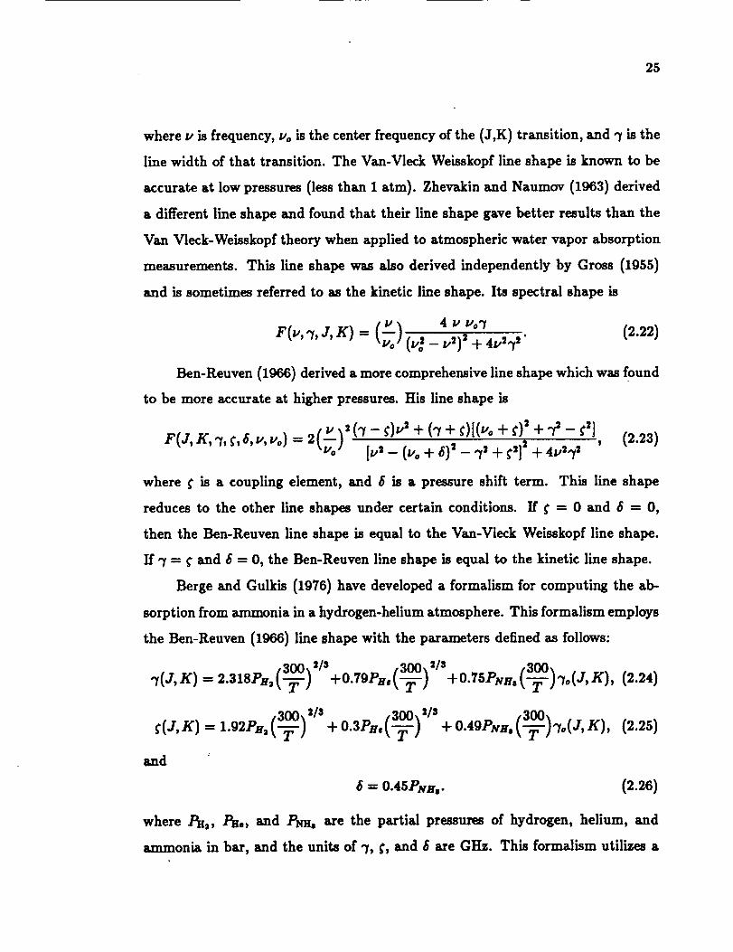
Ben-Reuven (1966) derived a more comprehensive lineshape which was found

to be more accurate at higher pressures. His lineshape is

r(J,K,_,_,6,.,.o) = 2_/ (2.23)[v,- (Vo+ - + + '

where f is a coupling element, and $ is a pressure shift term. This line shape

reduces to the other line shapes under certain conditions. If f = 0 and 6 = 0,

then the Ben-Reuven line shape is equal to the Van-Vleck Weisskopf line shape.

If "7 = f and 6 = 0, the Ben-Reuven line shape is equal to the kinetic line shape.

Berge and Gulkis (1976) have developed a formalism for computing the ab-

sorption from ammonia in a hydrogen-helium atmosphere. This formalism employs

the Ben-Reuven (1966) line shape with the parameters defined as follows:

+0.79P.. [-_'-) +O.75PlVHa(3--_-_)'7o(J,K), (2.24)"7(J, K)

_ ,300x'/' -300- '/s 0.49PNR,SOO, To(J,K),(.__.)f(J,K)=l.92Pn,[-T- ) +0.3PH,(T ) + (2.2s)

and

6 = 0.45PjvB.. (2.26)

where ]_I_, Pro, and Pss, are the partial pressures of hydrogen, helium, and

ammonia in bar, and the units of % f, and $ are GHz. This formalism utilizes a

26

correction factor (C) in Equation 2.19

in order to be consistent with the laboratory results of Morris and Parsons (1970),

who measured NHs absorption at 9.58 GHz in a high pressure H2/He atmosphere

at room temperature.

Recently, Spilker (1990) has derived new pressure and temperature depen-

dencies for the Ben-Reuven line shape based on high accuracy laboratory mea-

surements under simulated Jovian conditions from 9-18 GHz. However, the ex-

trapolation of this formalism to different pressures and frequencies can produce

unreliable results.

We have modified the parameters of the Ben-Reuven line shape in order to be

compatible with the results of this work as well as the work of Morris and Parsons

(1970), Steffes and Jenkins (1988), and Spilker (1990). This formalism employs

the Ben-Reuven line shape as described above with the pressure-broadened llne

width and coupling element given by

(30C)_'_/'-.t- 0.75P.S.,('-_)2/s-I - 0.6PN..(3--_)%(J,K) (2.28)•'I(J,K) = 1.69Ps,_ T ]

and

_ ,300,'/' (300_'/' ("_--)%(J,K), (2.29)f(J,K) = 1.35PB, (-_--) + 0.3PR, x-_-- / + 0.2Plvn,

respectively, where the units of -y and f are GH_. The pressure shift term, 5, is

the same as that of the Berge and Gulkis (1976) formalism (Equation 2.26). The

correction term (C) used in this formalism is equal to 1. Our formalism differs

only from the Berge sad Gulkis formalism.

Figure 2.6 shcsvs a graph of the four theoretical formalisms which are used

to compute ammonia absorption from I mm to 10 cm. The center frequencies, yo,

and self-broadened line widths, %, of the ammonia inversion resonances used in

all calculations are from Poynter and Kakar (1975).

27

10 zAmmonia absorption

! i Q i e , i | i

Zo

0

IOt

10o

10-1

lO-eIO o

vvw ................... 17 '_,,,,

BR-JS -"--_,..,,,."'"- """__,-..

"--.................."'"" VV "_-..

/ I I i I I I I I [ , i I I I | I A I

101 0 z

WAVELENGTH cm

Figure 2.6: Theoretically computed ammonia absorption for 90% H2, 10% He,

and 0.025% NHs, at 2 bars, and 200 K using the Van VIeck Welsskopf lineshape

(WW), Ben-Reuven lineshape u per Berge and Gulkls (BR-BG), Ben-Reuven

formM[sm as given in this paper (BR-JS), and Zhevakin-Naumov or Gross line-

ehape (ZN-G)

28

The absorption from the pressure-broadened submillimeter rotational lines

of NHs is significant at millimeter wavelengths. The absorption from the subm]l-

limeter lines is expressed by Equation 2.19 for J = 0,1 with

PIVH° K ,A(J,K) = 1.826 Vo(J,K)-_B(J, ) (2.30)

where

and

B(o,o)= 0.070(1- e-'8-'/T),

B(1,0)= 0.075(1- :".'/T):".6/L

(de Pater and Massie, 1985).

and C-- l.

(2.31)

(2.32)

B(1,1) = 0.0s3(1- :,,.,_):_.s/_. (2.33)

We use the kinetic line shape for F(3, K, % u, Vo)

2.2.5 Experimental Results and Interpretation

The results of the Ka-band and W-band NHs absorptivity measurements are listed

in Table 2.1. The theoretically-derived values for the Ben-Reuven, Van Vleck-

Weisskopf, and kinetic line shapes are also provided in tabular form.

The Ka-band results are presented graphically in Figure 2.7. Two sets of

measurements are shown. One set of measurements was conducted using a pre-

mixed, constituent analyzed gas mixture (NHs mixing ratio uncertainty - 4- 2_ of

its value). The gas mixture in the other set of measurements was mixed using the

thermocouple vacuum gauge (NHs mixing ratio uncertainty - 4- 20% of its value).

Also shown in Figure 2.7 are solid lines which represent the theoretically computed

absorption using the Van Vleck-Weisskopf line shape (WW), the Berge and Gulkis

(1976) modified Ben-Reuven line shape (BR-BG), our modified Ben-Reuven line

shape (BR-JS), and the Zhevakin and Naumov or Gross line shape (ZN-G). The

Van Vleck-Weisskopf line shape overstates the opacity of NHs by nearly a factor

29

Table 2.1: Measured and theoretical values of NHs absorption

Freq Date Press. a meas. a a a

(GHz) (atm) (dB/km) ZN/G VVW BR-BG BR-JS

t32.17 6/28/88 2.0 201±47 290.4 461.6 337.7

7/7/88 2.0 246± 45*

t32.89 6/28/88 2.0 254± 53 266.7 435.0 312.3

7/7/88 2.0 210± 54*t34.32 6/28/88 2.0 200± 34 226.7 388.6 269.0

7/7/88 2.0 146± 34*

t35.03 6/28/88 2.0 146_ 34 209.9 368.6 250.7

7/7/88 2.0 146± 36*

t35.75 6/28/88 2.0 173± 40 194.5 350.0 234.0

7/7/88 2.0 137_ 45*

t36.46 6/28/88 2.0 119± 40 180.9 333.5 219.1

7/7/88 2.0 146± 34*

t37.17 6/28/88 2.0 155± 40 168.6 318.4 205.7

717188 2.0 146± 47*t37.89 6/28/88 2.0 164± 40 157.4 304.5 193.5

7/7/88 2.0 137± 34*

t37.89 6/28/88 2.0 146± 40 147.4 292.0 182.5

7/7/88 2.0 100± 34*

t39.32 6/28/88 2.0 119± 34 138.2 280.5 172.5

7/7/88 2.0 109± 34*

_94.0 10/20/88 2.0 115±32' 42.3 350.6 117.0

10/20/88 2.0 109±32

_94.0 10/20/88 1.7 58±30* 30.8 253.9 84.7

10/20/88 1.7 36±30_94.0 10/20/88 1.3 0±30* 18.2 148.9 49.7

_94.0 10/20/88 1.0 0±30* 10.8 88.3 29.4

:_94.0 10/22/88 2.0 91±30' 42.3 350.6 117.0

10/22/88 2.0 91±30"

321.5

292.0

244.4

225.2

208.1

193.3

180.2

168.5

158.2

148.8

120.8

87.4

51.1

30.3

120.8

t88.34_ H2/9.81% He/1.85% NHa, T-203K

:_85.56% H2/9.37% He/5.07_ NHs, T:210K

*Measurements made with premixed, constituent analyzed mixture

3O

of 2, while the modified Ben-Reuvenline shape overstates the opacity of NHs by

an average of over 40%. At these frequencies, it is not clear which line shape (if

any) is most appropriate.

We have further evaluated theoretical line shapes by making use of our mea-

surements at higher frequencies where the line shapes are more distinct. Figure 2.8

shows the results of the 94 GHz experiment as compared to four theoretical line

shapes. At this frequency, it is clear that neither the VanoVleck Weisskopf line

shape nor the Gross line shape is appropriate. In Figure 2.9, we show an example

of laboratory measurements at centimeter wavelengths by Spilker (1990) compared

with our new formalism of the Ben-Reuven line shape. Our new line shape pro-

vides a good fit to laboratory measurements under a wide range of temperatures,

pressures, and frequencies.

Theory predicts that there should be a smooth transition from the Ben-

Reuven line shape to the Van Vleck-Weisskopf or Gross llne shape at some low

pressure. However, it is not known at what pressure this transition occurs. The

sensitivity of the millimeter-wave measurement apparatus used in our experiments

is not great enough to measure the absorption of ammonia under Jovian conditions

at pressures near or below 1 atm. In fact, we obtained no reliable Ks-band ab-

sorption measurements at 1 atm pressure. We obtained one reliable set of W-band

measurements at 1 atm pressure. The results are shown in Figure 2.10. Although

we measured no significant absorption at Iatm, the error bars give an upper limit

for NHs opacity. This upper limit is well below the Van Vleck-Weiaskopf theory

and more compatible with the Gross line shape at 1 atm. This is most likely due

to reduced coupling between individual lines at 1 atm pressure.

31

550

5OO

450

350

300250

0_n

< 200

150

IOO

Ammonia absorption under Jovian conditions

ZN-G

_0 ' '

30 31 32 33 34 35 36 37 38 39 40

FREQUENCY (GHz)

Figure 2.7: Measured and theoretical Ks-band absorption from gaseous NHs in

an 88.34°_ H=-9.81_ He-l.85_ NHs mixture at 210 K and 2 atm. o: Gases mixed

with thermocouple vacuum gauge; ,: PremLxed, constituent analyzed gas mixture.

32

Ammonia absorption under Jovian conditions

400 _ 1 _ T r

350

300

250

Z 200O

[..

O0_m 150

100

5O

V_

BR-JS

.................................... _b ...............................

BR-BG

ZN-G

0 -----------I- 1 1 I t

93.4 93.6 93.8 94 94.2 94.4 94.6

FREQUENCY (GHz)

Figure 2.8: Measured and theoretical W-band NH3 absorption in an 88.56%

H2-9.37_ He-5.07_ NHs mixture at 210 K and at 2 atm

33

220

200

180

6oi

m 1401

:" 120'

E

6O

Measured and theoretical ammonia absorptioni ! l i

BR-JS

ZN-G ....

4O VVW

20 , 1 , ,9 1O 11 12 13 14 15 16 17 IB

FREQUENCY (GHz)

Figure 2.9: Measured (Spilker, 1990) and theoretical NH: absorption in an 89.3%

H_, 9.92% He, 0.82% NH3 mixture at 273 K and at 8 atm)

34

zOP

Ammonia absorption under Jovian conditions

100 r r _ T 1

8O

6O

4O

2O

0

--2O

VVW

BR-JS

BR-BG

ZN-'G

-40 1 _---' ' ±--93.4 93.6 93.8 94 94.2 94.4 94.6

FREQUENCY (GHz)

Figure 2.10: Measured and theoretical W-band NHs absorption in an 88.56_

H2-9.37_ He-5.07_ NHs mixture at 210 K and at 1 atm

35

2.3 Measurement of Hydrogen Sulfide (H2S) Opac-

ity at G-band

Hydrogen sulfide (H2S) has several strong rotational lines at millimeter wave-

lengths (168, 217, and 300 GHz). The lines are pressure broadened by H2 and

He in the Jovian atmospheres. We have developed a system capable of measuring

pressure-broadening effects of H_ and He on the J_r,_lK£ _ - JK__K+I -- 20,2 -- 21,1

line at 217 GHz (1.4 mm). The laboratory configuration, procedure, and results

are described in the following sections.

2.3.1 Laboratory Configuration and Procedure

Because gaseous H2S is extremely opaque near the center of the rotational line

at 216.7 GHz, the extended path length provide by a resonator is not needed.

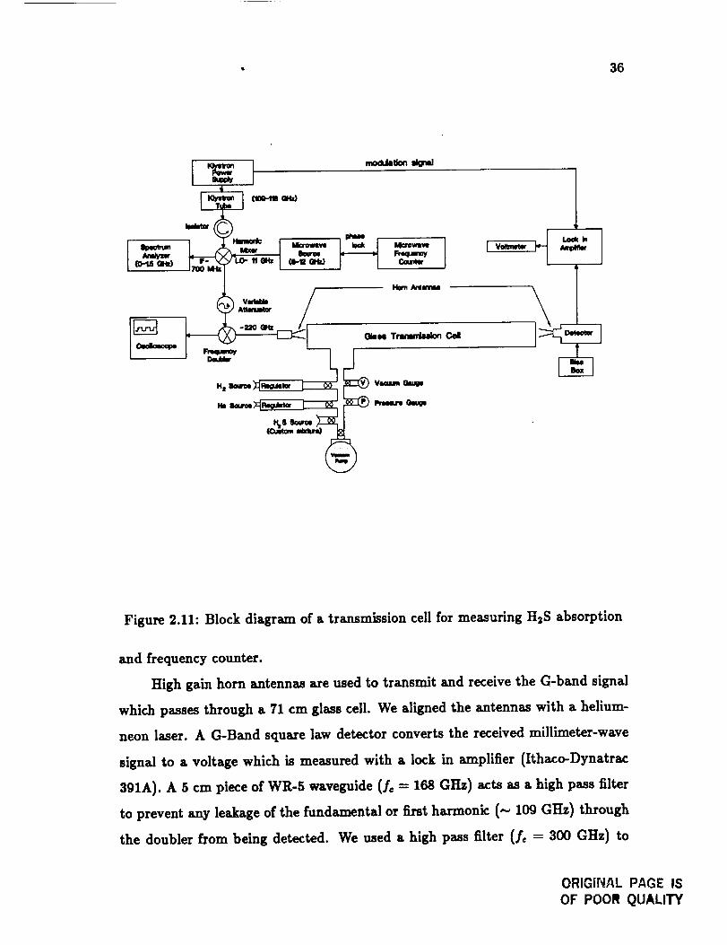
Hydrogen sulfide absorption can be measured with a transmission cell, a millimeter

wave source, and a detector. A block diagram of the system used to measure

H2S absorption is shown in Figure 2.11. The G-Band CW signal (._218 GHz)

is generated by doubling a W-Band (_109 GHz) klystron tube source (Varian,

Inc. VAT 692A2). The klystron power supply (Micro-Now Model 756) provides

1 KHz modulation by varying the voltage on the reflector of the klystron. The

variation in frequency using this technique is less than 0.5%. Since the pressure-

broadened line width of H2S is several GHz wide, absolute frequency stability is not

necessary. The modulation signal incident on the frequency doubler is monitored

with an oscilloscope. The klystron signal is sampled with a 20 dB coupler and

downconverted to an IF of approximately 800 MHz with a harmonic mixer. A

microwave source phase locked to a microwave frequency counter provides the LO

for the mixer. The frequency and stability of the IF signal is monitored with a

high resolution spectrum analyzer. The klystron frequency can be computed from

the precise measurement of the IF and LO frequencies using the spectrum analyzer

• 36

(ods Q_k}

I g)_dvmPm_r

-_T_ O0edm a_r_

Hm_c klcro_m___ Mxw/'LO- _ eHz t_m Ore)

_ _r_

J

L_kMlyre

Olee_l Tnmemle_ Gd

E

Figure 2.11: Block diagram of a transmission cell for measuring H_S absorption

and frequency counter.

High gain horn antennas are used to transmit and receive the G-band signal

which passes through a 71 cm glass cell. We aligned the antennas with a helium-

neon laser. A G-Band square law detector converts the received millimeter-wave

signal to a voltage which is measured with a lock in amplifier (Ithaco-Dynatrac

391A). A 5 cm piece of WR-5 waveguide (fc = 168 GHz) acts as a high pass filter

to prevent any leakage of the fundamental or first harmonic (_ 109 GHz) through

the doubler from being detected. We used a high pass filter (fc = 300 GHz) to

ORIGINAL PAGE IS

OF POOR QUALITY

37

measure the signal level of the third harmonic (-_ 327 GHz). The power from the

third harmonic was 30 dB down from the second harmonic. Thus, the detector is

measuring power from mostly the desired second harmonic (-_ 218 GHz).

A situation analogous to dielectric loading (described in the previous section)

occurs in a transmission cell measurement. Reflections occur at the cell boundaries

due to the different dielectric constants of the air outside the cell, gas mixture in

the cell, and lenses at the cell boundary. We first measured the power or voltage

on the detector with the H2S mixture in the cell. We then measured the power

with a gas mixture of 90% hydrogen and 10% helium in the cell. The indices

of refraction for the two gas mixtures (with and without H_S, respectively) at

STP are approximately 1.000183 and 1.000122. Reflections occurring at the cell

boundaries should be similar for both gas mixtures. In a less rigorous check, we

observed no difference between the signal level measured in the H2/He mixture and

in a mixture of 70% H=/30% air which has exactly the same index of refraction

as the H=S mixture. The absorption due to the hydrogen and helium mixture is

negligible. The attenuation due to the H=S mixture is computed from the ratio of

the voltages measured in the gas mixtures with and without H_S. This approach

ensures that the drop in signal level is due only to absorption and not to changes

in reflection at the cell interfaces.

A relatively high mixing ratio of H2S is needed in order to measure absorption

in the cell. The experiments take place at ambient temperature (296 K) and at a

total pressure of 2 arm. We used a pre-mixed, constituent analyzed gas mixture

(Matheson) in all experiments. This mixture consists of 78.79_ H=, 9.28% He,

and 11.93% H2S.

Because H2S is an extremely noxious and corrosive gas, various safety pre-

cautions are undertaken during the experiment. We used filtered gas masks and

safety goggles when handled the gas. All equipment coming in contact with the

H_S is constructed of stainless steel, glass, or plastic. The experiment takes place

38

indoors in a well ventilated area, and the gases are vented outdoors where they

are safely diluted by air.

2.3.2 Experimental Uncertainties

The main source of uncertainty in this experiment is power drift in the k]ystron

source. Power and frequency drifts occur as the temperature of the klystron varies.

We found that the k]ystron output power exhibited a sinusoidal drift even though

it was mounted on a large heat sink. The drift period is substantially longer

than the time required to make an individual measurement. By obtaining several

measurements, we can characterize the drift and minimize this uncertainty. The

overall uncertaintY in klystron power is approximately =I=7%. Other instrumental

uncertainties include uncertainty in the measurement of temperature (-t-1%) and

total pressure (-t-7_). The uncertainty in the mixing ratio of the gas mixture is

-I-2_ per stated component. The total uncertainty in the measured absorption

coefficient is the root sum square of the individual uncertainties.

2.3.3 Theoretical Characterization of H2S Absorption

In general, the opacity from a single absorption line at millimeter wavelengths is

expressed by

(_£)'/' [ 1 To)] F(v, vo, Av)cm_ I (2.34)a = N So ezp -1.439 E (_

where N is the number density in molecules/cm s, T is temperature in Kelvins, To

is a normalizing temperature (296 K), So is a normalized line intensity, E is the

lower state energy ]eve], and F(v, vo, Av) is the line shape. The line parameters

used in the computation of H2S absorption are taken from the GEISA (Gestion et

Etude des Spectroscopiques Atmospherique) line catalog (Chedin eta/., 1982 and

Flaud et a/., 1983).

39

The Van-Vleck Weisskopf (1945) line shape used in this calculation is

] (2.35)

where Av is the pressure-broadened line width, and all frequencies are in cm -x.

The pressure-broadened line width of H_S in an H=-He atmosphere is

Av = [AvH, Ps2 + Av_.Ps, + AVs2sPs2s] (2.36)

where Avs,, AvH,, and AV_2s are the hydrogen, helium and self-broadened line

widths of H_S. The temperature scaling exponent, n, has not been measured for

H2S. We assume a value of 0.67 for n, based on the values reported for the nitrogen-

broadened line width of H=O at 183 GHz (Waters, 1976). Because our measure-

ments are conducted at room temperature, the assumed value of n does not affect

our results. Moreover, the value of n does not significantly affect the line width

calculation when temperatures are extrapolated to lower temperatures occurring

in Jupiter's atmosphere. For example, changing the value of n to 0.3 (which we es-

timate to be a lower limit) at 200 K (the temperature near 2 bar on Jupiter) results

in a line width difference of less than 209{. Hekninger and De Lucia (1977) have

measured the self-broadened line widths of the -z +zd_, K' - J/t'_lA'+_ -- 20,2 - 21,1 line

at 217 GHz and report a value of AVH_S = 9.10 MHz/Torr (6.92 GHz/bar). Willey

cta/. (1989) have measured the helium-broadened line width of the 10,t - 11,0 hy-

drogen sulfide transition at 168.8 GHz and 295 K and found it to be 1.60 MHz/Torr

(1.22 GHz/Bar). We assume the same value of Av_. for the 20,2 - 21,1 transition.

2.3.4 Experimental Results

The measured H=S absorption at 2 atm and 296 K is shown in Figure 2.12. The

solid lines represent the theoretically computed absorption for several values of

A_a s. Visual inspection of Figure 2.12 suggests a value of AVH= approximately

equal to 2 + 0.5 GHz/Bar (2.6 + 0.7 MHz/Torr).

40

o

2.5

2

1.5

0.5

Hydrogen Sulfide Absorption

A_, '= 1 GI-Iz,/bar ' '

H2 ,...,_

e

!

/ \q _r _

O I I I i i ,, I i

200 205 210 215 220 225 230 235 240

FREQUENCY (GHz)

Figure 2.12: Measured and theoretical G-Band absorption from gaseous H2S in

a 78.79_ Hs, 9.28_ He, 11.93_ H2S mixture at 2 atm and 296 K. Theoretical

absorption using the Van V]eck-We]sskopf line shape for various Avls2 between 1

and 5 Gtts/bar.

41

CHAPTER 3

Modeling of the Jovian Atmospheres

In the last chapter, we developed formalisms for computing the absorption from

gaseous NHs and H2S. In this chapter, we apply the new expressions to a radiative

transfer and thermochemical model of the giant planet atmospheres. This chapter

begins with an explanation of a thermochemical model which is used to predict

the distribution of volatiles (NHs, H_S, H_O, and CH4) in the giant planet atmo-

spheres. Section 3.2 follows with the theory of radiative transfer as it is used to

compute the radio emission from the giant planets. Section 3.3 describes the pa-

rameters of the radiative transfer model in detail. In this section, we also develop

new expressions for computing the absorption from other opacity sources. In Sec-

tion 3.4, we adjust the parameters of the radiative transfer and thermochemical

models for each the four Jovian planets. Using a forward modeling approach, we

compare the modeled emission of each planet with its observed emission.

3.1 Thermochemical Modeling

The composition of the Jovian clouds cannot be readily determined by present

observational techniques. However, the composition of clouds can be predicted

with thermochemicaJ models. Weidenschilling and Lewis (1973) developed some

of the earliest thermochemica] models of the giant planets. Their models were

based on a solar mix of elements. Recently, thermochemical models have been

combined with radiative transfer models and used to predict the emission from

42

the giant planet atmospheres(see,e.g., Atreya and Romani, 1987or Briggs and

Sacket, 1989). We will use the thermochemica] models in a similar approach. We

will estimate the distribution of cloud forming constituents in the giant planet

atmospheres and use the distributions in a radiative transfer model to predict the

radio emission from the giant planets. We will also use the thermochemica] models

to estimate cloud bulk densities which will be used in the computation of cloud

opacity.

The atmosphere in the thermochemical model is composed of discrete homo-

geneous layers. The thermochemica] model begins deep in the atmosphere where

a starting temperature and pressure have been previously established (see Sec-

tion 3.3.1). A step dP is taken, and the average temperature and pressure are

computed. A check is made to see if condensation has occurred.

The saturated vapor pressure for a single constituent over a single phase is

in(P) = -_ + a, + as in(T) + a,T + asT'. (3.1)

We use values of the coeflRicients _ for liquid and solid NHs and H20 from Briggs

and Sacker (1989). The values of al-2 (as-6 = 0) for liquid and solid CH, are from

de Pater and Massie (1985). Although both NHs and H_S dissolve in aqueous H20

cloud drops, the net effect on the millimeter-wave opacity, latent heat, and depres-

sion of the freezing point is small (see, e.g., Grossman, 1990 or Briggs and Sacket,

1989). Therefore, we will consider only a pure H20 cloud in the thermochemi-

ca] mode]. The coefficients a_ for solid H2S were derived from recent laboratory

measurements by Kraus eta/. (1989).

Gaseous NHs and H2S combine to form solid ammonium hydrosulfide (NH4SH)

in the reaction

NH,(gaa) + H,S(gas) _ NH, SH(solid), (3.2)

where the equilibrium constant K is related to the saturated partial pressures of

43

NHs and H_S by

10834

ln(K) = In(PNHsPH2s) = 34.151 T ' (3.3)

where P_H8 and PH=s axe the partialpressures of NHs and H_S in bar. The value

of K could be overestimated by a factor of 3 in the worst case (de Pater eta/.,

1989). Therefore, the NH_SH cloud could form at deeper levelsin the atmosphere

(higher pressures). Since no additional laboratory data isavailableat this time,

we willuse Equation 3.3.

Ifcondensation has occurred, the incremental change in the mixing ratio of

the condensate iscomputed. The mixing ratioor molar concentration (Xk) for an

ideal gas is

x.= (3.4)

where Pk isthe partialpressure of gas k, and P isthe mean pressure. The change

in mixing ratio,dXk, isfound by differentiatingEquation 3.4:

1 Pt

dXj, = -_dP, - -_ dP.

Substituting the Clausius-Clapeyron equation,

(3.5)

dP LP

d-'-T-- RT'''_' (3.6)

into Equation 3.5 yields

L_,Pk a- LkPhdXi, = p_*_l p= dP. (3.v)

The incremental change in the mixing ratios of NHs and H2S resulting from the

formation of the NH4SH cloud is

PN]asPH_s 10834 2 dp].dX_m, = dX_s = [P(P-'_s _s) ] [--_dT -(3.8)

The saturated vapor pressure for a single constituent over a single phase is

{gl

ln(P) = -_ + a2 + as In(T) + a,r + asr=. (3.9)

44

We use values of the coefficients a_ for liquid and solid NH3 and H=O from Briggs

and Sacket (1989). The vaJues 0f al_= (as-5 = 0) for liquid and solid CH4 are from

de Pater and Massie (1985). Although both NHs and H=S dissolve in aqueous H20

cloud drops, the net effect on the millimeter-wave opacity, latent heat, and depres-

sion of the freezing point is small (see; e.g., Grossman, 1990 or Briggs and Sacket,

1989). Therefore, we will consider only a pure H=O cloud in the thermochemi-

cal model. The coefficients a_ for solid H2S were derived from recent laboratory

measurements by Kraus et al. (1989).

Gaseous NHs and H_S Combine to form solid ammonium hydrosulfide (NH, SH)

in the reaction

NHs(gas) + H,S(gas) _ NH4SH(solid), (3.10)

where the equilibrium constant K is related to the saturated partial pressures of

NHs and H_S by

10834

In(K) = ln(Pmt, PR, s) = 34.151 r ' (3.11)

where PNH8 and PH2s are the partial pressures of NHs and H=S in bar. The value

of K could be overestimated by a factor of 3 in the worst case (de Pater eta/.,

1989). Therefore, the NH4SH cloud could form at deeper levels in the atmosphere

(higher pressures). Since no additional laboratory data is available at this time,

we will use Equation 3.8.

The cloud density is computed according to Weidenschilling and Lewis (1973)

D = 100 dX_ m___P-= g/cm s (3.12)dPTR

where P is the mean pressure of the layer in bar, T is the mean temperature in

kelvins, dP is the difference in pressure between the top and bottom of the layer,

dX_ is the change in mixing ratio of condensate/c, rn_ is the molecular weight of

the kth condensate, and R is the universal gas constant. The resulting cloud bulk

densities and vertical distributions of the cloud forming constituents are integratedv

into the radiative transfer model which is described in the following section.

45

3.2 Theory of Radiative Transfer

In this section,we develop various forms of the radiativetransfer equation. The

equations are used to compute synthetic brightness spectra of the giant planets.

We also explore the potential effectof the oblate shape of the giant planets on

their radio emission.

3.2.1 The Radiative Transfer Equation

The Planck radiation law relatesthe brightness radiated by a black body (B,,(T))

to itsphysical temperature (T) in kelvinsand frequency (u) in Hz as follows:

Bj,(T) = c'[exp(_) - 1]' (3.13)

where c is the speed of light (2.998 × 101° cm/s), h is the Planck constant (6.63

× 10 -s4 J s) and k is the Boltzmann constant (1.38 x 10 -2s J/K). The units of

By(T) are watts per square meter per hertz per steradian (Wm-2Hz-lsr-X).

The radiative transfer geometry for a planet is shown in Figure 3.1. The

zenith angle, 0, is defined at a given point on a constant pressure surface of the

planet. It is the angle between the observer's line of sight to the planet and the

local normal to the surface at that point. The quantity # is the cosine of the zenith

angle. The radiative transfer equation gives the total brightness emitted at the

top of the atmosphere (z = 0) along a ray in the direction # as follows:

where z is the depth as measured from the top of the planet (z - 0), and a_(z) (in

optical depths per unit length) is the total absorption coet_icient or the sum of all

of the absorbing processes at the depth z and at frequency v. The total brightness

can also be expressed in terms of a weighting function, l#v(z, #):

46

line of sight

Normal

zenith angle _'-

/_= cose /

/to isobaric surface /

"r=0

Atmospheric layers

Figure 3.1: Sketch of the zenith angle of a planet.

The weighting function provides a representation of which altitudesare contribut-

ing most to the emission at a particular frequency. Another term commonly used

in radiative transfer modeling isthe verticaloptical depth, r, which isdefined as

(3.16)

Substituting Equation 3.13 in Equation 3.11 yields an alternate form of the radia-

tive transfer equation:

J0t)'B"T(')" • d,B.(T,#)= exp(-_)-_-. (3.17)

The absorption coefficient for gaseous molecules is a function of temperature,

pressure, and frequency. The temperature, T, and pressure, P, may be related to

depth in the atmosphere, z, by the hydrostatic equation,

dP -- p g dz, (3.18)

47

and the equation of state,

p -=-- m

pTR

m(3.19)

The disk-averaged brightness of a planet, By(To), results from the integration of

Equation 3.11 or 3.14 over all angles of incidence using

B,,(TD) = 2 [' Bv(T,p)pd#. (3.23)Jo

3.2.2 Disk-averaged Brightness

is found by inverting the Planck function:

hvTB=

k In/rh,,,1 1)"_t_g_-_j +(3.22)

which yieldsRT

dz = (-_-_ap )dP, (3.20)

where R is the universal gas constant (8.3143 x 107 erg k -1 tool-l), _ is the mean

molecular weight of the atmosphere, and g is the acceleration due to gravity. Using

Equation 3.17, the absorption coefficient at frequency v can be written simply as

a function of depth z.

The integral over r in Equation 3.14 is evaluated by modeling the atmosphere

as a finite number of discrete layers. The average temperature, pressure, and

altitude are specified at each layer. The integration begins at top of the atmosphere

(P=10 mbar, r = 0, z = O) .and is terminated when r reaches a value of ro = 5

optical depths:

Vo=5

B,,(T, I_) = Z: + (3.21)t'=0

where the last term is a correction factor which accounts for the brightness con-

tribution from altitudes below the cutoff altitude, to. The correction assumes that

the temperature is constant below the cutoff altitude.

Radio astronomical observations of the planets are commonly reported in

terms of the temperature of an equivalent blackbody that would produce the ob-

served brightness. This temperature, TB, is called the brightness temperature. It

48

Combining Equations 3.14 and 3.20, the disk-averaged brightness is expressed by

(3.24)

Spherical Approximation

If the shape of the planet is a sphere, the integral over/_ may be simplified to a

single integral (Goodman, 1969) by making use of the exponential integrals of the

form

Substituting y = 1/l_, Equation 3.21 becomes

or

(3.25)

(3.26)

(3.27)B,.CTol- B,, dE C,-I.The exponential integral is evaluated numerically.

Oblate Grid Model

In order to test the spherical approximation, the integral over/_ in Equation 3.20

can be evaluated by constructing a grid of the projection of the planet against the

sky. The grid is made up of a finite number of rectangular elements which form the

oblate shape of the planet. A grid of Jupiter is shown in Figure 3.2. The grid is

more finely spaced at the edges of the planet where the limb darkening is greatest.

The brightness temperature is computed at each point (from Equations 3.11 or

3.14) and weighted according to the fractional area which it covers on the projec-

tion. The disk-averaged brightness is the weighted sum of the brightness over all

elements:

Ts(disk - averaged) = fxf;,TB(x,y)dx dyfxJ',dx dy " (3.28)

49

O0 0.2 0.4 0.6 0.8 I .2

Figure 3.2: Grid of Jupiter.

5O

A

7/

A

rl ^r

Z

Figure 3.3: Geometry of an oblate spheroid.

The grid coordinate system is shown in Figure 3.3. The disk of the planet is

projected onto the (_,_)) plane. The line of sight from the observer to the planet is

in the direction _. Each (z,y,z) refers to the coordinate of a point on the surface

of the planet that is projected onto the (_,_) plane.

The surface or radius of a Darwin-de Sitter spheroid is a function of the

planetocentric latitude _a (Zharkov and Trubitsyn, 1978):

r(O) = 1 + 50 -b Z I_iP, i(¢os(_)), (3.29)i=1

where P2i is the Legendre polynomial of degree 2i, b2i are coefficients which are

related to the zonal harmonic coefficients J,_, and

= - 4,', (3.30)

The planetographic latitude, _ is related to the planetocentric latitude _w by

q_= q_'-I- ar ct cn L-_-_ ) . (3.31)

51

The planetocentric longitude, _, is

"-and

z = ,,/(,'(4,) - (3.33)

The 1 bar surfaces of Jupiter and Saturn are shown in Figure 3.4. For Uranus and

Neptune, the ellipticity is less than 2%.

The value of @ at the surface of the planet for a point (x, y) on the projection

can be computed using Newton's method

,-C¢,.)co,,C_.) -• .+,(_, b2,) - _. - d,C_.)eo,(_.) - ,(_.),/nC_.)"

(3.34)

The cosine of the angle between the line of sight (_) and the local vertical or

normal C_) is equal to # for a sphere as well as an oblate spheroid:

p = ¢_. _ = eos(qb) 8in(_). (3.35)

For a sphere, _b= _'.

The gravitational field of the planet is expressed in terms of radial (g,) and

latitudinal (g÷) components (see, e.g., Lindal et o2, 1985)

= _,g, + fj'÷g÷, (3.36)

where ur and _÷ are unit vectors in the radial and latitudinal directions, respec-

tively. The vector components are

GM

g,..(,,.,¢,)= ,, t- -_-GM,=,_(2i + 1)J2,(R)"P2,(,in_b) + w2r[1 - P2Csinq_)] (3.37)

and

GM _ (R] 'idPzi(*in_) 1 z dPz(sinq_)g÷(r, qb)-- -_ Jz, x-_/ _ _ r d_ "" ' (3.38)°--.

where G is the universal gravitational constant, M is the mass of the planet, J2i

is the 2ith zonal harmonic coefficient, R is the radius normalized to the J2¢, P2¢ is

52

1.5

0,5

Jupiter's Oblateness

< - X

! :i

i / :

/

o

-0.5

-1

0

//

/

/

..... _ ............. TJ

/

53

the Legendre polynomial of degree 2i, _o is the angular velocity, r is the distance

to the center of mass, and _ is the planetocentric latitude. The planetocentric and

planetographic latitudes are related to the gravitational components by

q_= r_'- arctanCg,/gr ). (3.39)

We found that the variation in gravity over the disk of the planet did not signifi-

cantly affect the computed brightness temperature. Therefore, we use a constant

value of g equal to the area weighted average.

The calculation of the disk-averaged brightness temperature is computation-

ally intensive. However, the amount of computation can be significantly reduced

as follows: First, construct a table of the brightness temperature (Tv) as a func-

tion of _, from p = 0.1 to I (TB = 0 at p -- 0) using Equation 3.14. Then compute

the value of/_ at each point on the (z,y) grid. Use a table look up with linear

interpolation to find the brightness temperature at each point on the grid. Use a

weighted sum to find the disk-averaged brightness temperature (Equation 3.25).

Since the brightness as a function of/_ is nearly linear, the brightness temperature

need only be computed for a few values of/, (we use approximately 10). The

symmetry of the z and y axes further decreases the amount of computation since

disk-averaged brightness need only be computed for one quadrant of the visible

hemisphere of the planet.

In order to test the accuracy of the finite element grid, the total brightness

was evaluated on a circular grid and compared with the exact solution using Equa-

tion 3.23. The difference between the two methods was approximately 0.6% in the

worst case.

Finally, we computed the disk-averaged brightness with the finite element

oblate grid and compared it with the spherical approximation. The difference

between the two methods for both Jupiter and Saturn was less than 1% for wave-

lengths between I mm and 10 cm. Since other uncertainties in the radiative trans-

fer model are much larger than 1% (e.0., uncertainty in the absorption coefficient),

54

the useof the spherical approximation is justified.

3.3 Parameters of the Radiative Transfer Model

(RTM)

The parameters of the radiative transfer model (RTM) are the temperature-pressure

profile, absorption profiles of the absorbing constituents, and the abundance pro-

files or vertical distributions of the absorbing constituents (abundance as a function

of altitude or pressure). We use a forward modeling approach, in which we vary the

parameters of the RTM in order to obtain good agreement between the modeled

and observed spectra.

Radiative transfer models are complex because they involve multiple param-

eters. In most cases, a unique solution does not exist. Fortunately, some of the

variables may be constrained. The laboratory measurements of NHs absorption

described in Chapter 2 are very important, because they eliminate one of the vari-

ables in the radiative transfer model. Measurements by the Voyager spacecraft

help to constrain other variables such as the temperature-pressure profile. In the

following sections, we discuss the parameters of the RTM in detail.

3.3.1 Temperature-Pressure Profile

The computation of the temperature-pressure profile begins deep in the atmo-

sphere of the planet where a starting temperature and pressure are specified. A

step, dP, is taken and the corresponding change in altitude, dz is computed from

Equation 3.17. A check is made to see if condensation has occurred. If so, the

lapse rate is equal to the saturated adiabatic lapse rate. The saturated adiabatic

lapse rate is found by solving the equation of energy conservation for the adiabatic

55

expansionof one mole of gas as follows:

C_,dT + _dP + LkdX_ = 0, (3.40)

(see, e.g., Atreya and Romani, 1985) where T is temperature, P is pressure, R is

the universal gas constant, dX_ is the change in mixing ratio of gaseous condensate

k, Lk is the latent heat released on condensation for the kth condensate, and 6'? is

the specific heat. Substituting Equations 3.7-3.8 into Equation 3.38 yields a form

of the saturated adiabatic lapse rate:

_ + _(X,os'X..,)LRx_]dT = mg [1+ _(E.L.X. (xs,s+x._,,) )J (3.41)

dz Cp [1 + _ (_, LIX, + (xs,s+x...)

where dz is the layer thickness, _ is the weighted or mean molecular weight

of the atmosphere, g is the gravitational acceleration, and Lax is the heat of

reaction for the formation of NH_ SH, and _ is the weighted or mean specific heat

of the atmosphere. Using the Clausius-Clapeyron equation (Equation 3.6) and

Equation 3.1, the latent heat released per mole is expressed by

L = -a, + asT + a4T 2 + 2asT s,

where the a_ are the same coefficients as described in Section 3.1.

rate:

(3.42)

If no condensation occurred, the lapse rate is equal to the dry adiabatic lapse

dT _g (3.43)dz c,

The temperature-pressure profile is computed iteratively and constrained to meet

the deepest level probed by the Voyager radio occultation experiments.

A constant specific heat is used for all constituents except H2. The specific

heats are shown in Table 3.1 (Grossman, 1990). The specific heat of hydrogen is

explicitly dependent on the ortho.para ratio (orientation of the hydrogen atoms

in the molecule) which is dependent on temperature. We will assume, as have

others (see, e.g., de Pater and Massie, 1985 or Briggs and Sacket, 1989), the

56

Table 3.1: Specific heat of atmospheric constituents

Atmospheric Constituent Cp/R

He (Helium) 2.503

CH. (Methane) 4.296

H20 (Water vapor) 4.018

NHs (Ammonia) 4.459

H2S (Hydrogen Sulfide) 4.013

frozen equilibrium or intermediate case for the specific heat of hydrogen (see, e.g.,

Wallace, 1980). The effect of the ortho-para ratio of hydrogen may slightly alter the

temperature-pressure profile. However, we will consider the temperature-pressure

profile to be a constrained variable in the radiative transfer model.

3.3.2 Opacity

In the last section, we constrained one of the variables of the RTM. In this section,

we will examine the opacity from various atmospheric sources in detail. By making

use of all of the available laboratory measurements, we will constrain this variable

to a large extent. However, some uncertainty in the computation of opacity still

remains.

NH3 Absorption

The new formalism of the Ben-Reuven line shape described in Section 2.2.4 pro-

rides the best fit to laboratory NHs absorption measurements obtained at radio

wavelengths. This formalism will be used to compute the absorption from gaseous

57

NHs in the radiative transfer model.

H2S Absorption

The absorption from H2S is computed as in Section 2.3.3. We use the line param-

eters from the GEISA catalog (Chedin eta/., 1982) for 80 lines with frequencies

up to 600 GHz. The computed absorption from H2S under Jovian conditions from

1 to 600 GHz is shown in Figure 3.5.

Pressure-Induced Absorption

Another source of opacity in the radiative transfer model is pressure-induced ab-

sorption from molecular hydrogen pairs (i.e., H2-H2, H2-He, and H2-CH4). Pressure-

induced absorption is caused by the transient dipole which is induced by inter-

molecular forces in pairs of colliding molecules. This effect is a large source of

opacity at millimeter wavelengths for Uranus and Neptune where ammonia is de-

pleted.

Goodman (1969) developed a simple expression for calculating the pressure-

induced absorption from H_-H2 and H2-He pairs at radio wavelengths:

= PpI2[PH2 ÷ 1.7 PHe cm -1, (3.44)_H2

where PH2 and Pso are the partial pressures of hydrogen and helium in atm,

and :_ is the wavelength in cm. We compare this expression to the extrapolation

of an empirical formalism developed from more recent laboratory data taken at

infrared wavelengths (Bachet eta/., 1983 and Dore eta/., 1983). The pressure-

induced absorption is computed from the computationally intensive six-parameter

empirical model given by Borysow eta/. (1985). We fit new parameters for the

temperature and pressure dependencies in the Goodman (1969) expression to the

Borysow eta/. (1985) model. We added a term to account for H2-CH4 absorption.

We optimized the parameters for temperatures and pressures corresponding to

58

10-4

10-5

010, e

0

Z 10-7

o lO-Sra'2

10-9

Hydrogen Sulfide Absorption

10-s010 0 101 10 z 10 3

FREQUENCY GHz

Figure 3,5: The computed absorption from gaseous H,S under $ovian conditions:

Xs2 -- 0.90, Xa, = 0.10, Xs, s = 3.35 x 10 -5, P=2 atm, T=200 K.

59

Jupiter's atmosphere. The new expressionis

o,.= ,o-,,.,,,,.,,, ÷ T '"' _ ,273_s's41

+ 9.322_CH, iv-) J"

(3.45)Graphs of the three formalisms are shown in Figure 3.6 for 30 and 300 GHz (1

cm and 1 ram). Our new expression deviates from the Borysow formalism by less

than 1% for pressures less than 10 bar. At higher temperatures which correspond

to pressures greater than 100 bar in the Jovian atmosphere, our new expression

deviates from the Borysow formalism by approximately 10%.

HlO Absorption

Goodman (1969) developed an expression for computing water vapor absorption

based on the experimental data which was available at that time. This expression

employed a Van Vleck-Weisskopf line shape for the rotational line at 22.235 GHz

and a residual term for the remaining rotational lines which occur at higher fre-

quencies.

We have developed a new expression for water vapor absorption under `jo-

vian conditions which is based on more recent laboratory data under terrestrial

conditions. The parameters for the water vapor lines are summarized by Ulaby et

a/. (1981) from a more detailed compilation by Waters (1976). This calculation in-

cludes ten rotational lines with frequencies up to 448 GHz. The kinetic line shape

is used in this calculation along with an empirical correction term derived by Gaut

and Reifenstein (1971). Our expression is essentially the same as that described in

Ulaby et a/.(1981). The term P representing the pressure in the earth's nitrogen

and oxygen atmosphere is replaced by (0.81Ps2 -I-0.25Pae) to reflect the broadening

characteristics of the ,Jovian atmosphere. Figure 3.7 shows a comparison between

the Goodman (1969) expression and our expression for pressures of I and 6 bar.

60

"o

"o

o

Zc)

C)

5

010

xlO -a Pressure Induced Absorption at 30 GHzr i i i i i ,

i I I .A I I i I

20 30 40 50 60 '70 80 90 100

PRESSURE bar

xl0 -e Pressure Induced Absorption st 300 GHz

I

0i0 20 30 40 50 60 70 80 90 100

PRESSURE bar

Figure 3.6: Computed pressure-lnduced absorption from H2-H2, H2-He, and

H_-CH4 pairs as a function of pressure Jup|ter_s atmosphere at 30 and 300 GHz;

Solid line: our expression; dot-dash line: Borysow et d. (1985) model; dashed line:

Goodman (1969) expression.

61

tJ

q_

o

0u_

10-_

lO-e

Water Vapor Absorption at 2 barsi i i , i I i I i i i i i , i ! I -

A A

this work .................._

I I I t | ,[ I ! I I t & I , , i ,

10 0 .0_

PRESSURE bar

10-2

o

lO-e

0r/2

Water Vapor Absorption at 6 bars

B

Goodman (1969) _..__.._.

I I I I I I I l I I I I _ i i . .

10 o O]

PRESSURE bar

Figure 3.7: Comparison between Goodman's expression and our expression for

H20 absorption with Xs= = 0.9, Xs, = 0.1, and Xu=o = 1 x 10-e; A: 1 bar, 150 K;

B: 6 bar, 300 K; Solid ]ine: our expression, dot-dash: Goodman (1969) expression.

62

Absorption from other minor constituents

Lellouch eta/. (1984a,b) and Lellouch and Destombes (1985) have completed an

extensive study of the detectability of minor species in the atmospheres of Jupiter

and Saturn at millimeter wavelengths. They considered absorption from phosphine

(PHs), hydrogen cyanide (HCN), carbon monexide (CO), and many other more

complex molecules. The abundances of these molecules in the Jovian atmospheres

are quite small. Emission cores arising from molecules such CO or HCN in the

stratospheres of Jupiter or Saturn might be detectable. However, their net effect

on the millimeter continuum is negligible. In fact, the only molecule capable of

providing a significant amount of opacity is PHs. We will compute PHs absorp-

tion using the parameters from the Poynter-Pickett catalog (1981) and assuming

the same line width as that of H2S. We will neglect the absorption from other

molecules.

Cloud Absorption

Another potential source of opacity at millimeter wavelengths is scattering and

absorption from cloud condensates. We have developed a computer program for

computing cloud transmissivity and reflectivity using the two-stream approxima-

tion. Our cloud model is described in detail below. In the following section, we

use this model to compute potential cloud rettectivities and transmissivities for

Jupiter.

The volume extinction coefficient for cloud condensates is the sum of its

volume absorption and scattering coefficients

Jr, _Vo

= = ,:.+ ,,. =E +F_,Q.(",). (3.46)i----I i-----1

where Q, and Qo are the scattering and absorption cross sections, respectively, N_

is the number of particles per unit volume, and r_ is the radius of the ith particle.

In the Rayleigh approximation, the scattering and absorption cross sections

63

are simply

and

respectively,where

2_1 6 i=Q.-'-_X I K (3.47)

_2

Q. = -7-×'xm(-K), (3.48)

_- _

fi2-1 g-1

fi_+2 _+2'

2_r

)_'

= g - jc n,

e,= n -.ik,

E_ -- n $ -- k $ ,

en = 2nk,

(3.49)

(3.50)

(3.51)

(3.52)

(3.53)

(3.54)

(3.55)

r is the partich radius, A is the wavelength in the same units, fl is the complex

index of refraction, and _ is complex dielectric constant. The Rayleigh scattering

approximation is acceptable for I RX I< 0.5 (Ulaby et al., 1981). If I fix I> 0.5, a

full Mie (1909) calculation should be performed.

If the absorption cross section is much larger than the scattering cross section,

Equation 3.44 reduces to a simple form:

¢zdo=l = I¢, = p,_ • (e -f- 2)' -F en:' cm-l' (3.56)

(Battan, 1973) where p is the density of the condensation particle (in g/cmS), M

is the bulk density of the cloud in the same units, _ is the wavelength in cm.

If the scattering cross section is comparable to the absorption cross section, a

more complex model is needed. In this case, the volume absorption and scattering:

coefficients are

ii'_, = p(r)Q,(r)dr (3.57)

64

and

= , p(,)Q,(,)dr, (3.58)respectively, where r is the radius of the cloud particle, p(r) is the drop-size dis-

tribution, and rl and r2 are the lower and upper limits of the drop radii in the

cloud. The phase function asymmetry, g, is

1/'2 G p(r) Qo(r)dr, (3.50)g "- K° Jrz

where G is the fraction of power scattered in the forward direction. We assume

that the scattering is from spherical particles, so that G is determined from the

Mie coefficients (see e.g., Gasiewski, 1000).

The uncertainties in modeling the cloud absorption are very large and arise

from several sources. One uncertainty is the cloud bulk density. We estimate the

densities with the thermochemical model described in Section 3.1. Romani (private

communication, 1990) suggests that the actual cloud densities on the planets may

be a factor of 5 less than those predicted with equilibrium condensation models

based on studies of the earth's clouds. Therefore, the cloud bulk density will be a

variable in the computation of cloud opacity. Another uncertainty in calculating

cloud opacity is the complex index of refraction of NH3 and NH4SH ice. The

complex index of refraction for NHs ice has been measured at infrared wavelengths

by Sill eta/. (1980). We use a value of 1.3 for nNHs (Sill eta/., 1980), 1.74 for

nNS, SU (CRC, 1980), and 1.78 for neao ice (Ulaby, 1981). The value of n should

not differ significantly from infrared to millimeter wavelengths. However, the value

of k is frequency dependent. We will assume _m, and k_m,SH to be variables. For

H20 ice,a_

ku,o = (3.60)(Grossman, 1990) where a is the absorption coefficient. At _ = 1 mm, k82o =

0.00035.

Finally, there is a large uncertainty in the cloud particle size and distribution.

West eta/. (1986) have given a summary of constraints on the particle sizes of

65

Jupiter's clouds based on a compilation of available observations. There is evidence

for a stable layer of particles having effective radii of i pm or smaller at pressures

from 0.2 to 0.7 bar. A layer of larger particles (- 3 - 100/_m) may exist neax 0.7

bar primarily in Jupiter's zones. This cloud is thought to be a mixture of NHs ice

and chromophores (although there is no direct evidence). Bjoraker eta/. (1986a,b)

used a massive absorbing cloud (greybody with T _ 3) at 2 bar in order to explain

observations at 5/_m. This second cloud is thought to be NH4SH ice and/or H_O

ice. There are no estimates of particle sizes for this cloud.

We have assumed the particle-size distribution to be a modified gamma dis-

tribution (Deirmendjian, 1969):

pC,)= a,° (3.61)

where a, b, a, and "_ are shape factors. We assume two of the shape factors to be

similar to those of a cirrostratus cloud:

a = 6, _ = 0.5, (3.62)

(see, e.g., Ulaby eta/., 1981). The remaining shape factors b and -_ axe determined

by specifying a mode radius (re) and bulk density M for the cloud. The mode

radius, re, is defined as the radius at which the distribution p(r) is at a maximum.

The shape factors may be written in terms of the mode radius,

r:- _-, (3.63)

and the bulk density, M,

paz"M = g/cm s, (3.64)

where

,,+4

,y

p is the density of the condensate, and 1_ is the gamma function.

(3.65)

66

The radiative transfer problem is simplified by assuming that radiation is

scattered in only the forward and backward directions. The cloud is assumedto

be made up of discrete homogeneous layers. The reflection and transmission for a

layer of thickness dz are

and

r=- 1 + v_- _Tcoth(a= dz)(3.66)

vrf- csch(ao dz)t, = , (3.67)

I -i- x/T-L-_coth((_c dz)

respectively (Gasiewski, 1990), where a= is the mode power attenuation coefficient

(3.68)

is the back-scattering albedo

--w= It.l, , (3.69)/Ca -t" ,K,.b

I¢= includes both gaseous absorption and absorption from cloud particles, and _0b

is the back-scattering coefficient

1-glc.b ----.'c._-- (3.70)

If the reflectivity and transmissivity of two adjacent layers (a and b) are specified,

the combined reflectivity and transmissivity of both layers are

tartta

r=i = r. + 1 - r=rt (3.71)

and

t,tb

t_ -- 1 - r, rb' (3.72)

(e.g., Paltridge and Platt, 1976) respectively, for downwelling radiation. A similar

set of equations applies to upwelling radiation.

Once the reflectivity and transmissivity are known, the brightness temper-

ature at/_ - 1 can be roughly estimated using the following approach: Suppose

67

that there is a cloud at pressure Pc and temperature To, with reflectivity rec and

transmissivity trc, and that the zenith optical depth above the cloud is rl. The

total brightness or emission at _ - 1 is the sum of the emission from the atmo-

sphere above the cloud, emission from the cloud itself, emission reflected by the

cloud, and emission from below the cloud:

By(T, _ -- 1) --fo"_Bv(T(_)) exp(-,)d, + (1 - rec - trc)B_(Tc) exp(-rl)+

3.3.3 Vertical Distributions of Opacity Sources

In the previous two sections, we constrained two of the three parameters of the

RTM to a large degree. This leaves the vertical distribution of opacity sources

as the main variable in the model. The gaseous constituents are well mixed in

the deep atmospheres of the giant planets. Some of the gaseous constituents will

be destroyed by photolysis or condensation at higher altitudes. We estimate the

vertical distribution of the cloud forming constituents NH3, H2S, and H20 using the

thermochemical model described in Section 3.1. The actual distributions are more

complex; they exhibit latitudinal variations due to upwelling and downwelling, and

some of the gaseous constituents might be super-saturated (see, e.g., de Pater et

a/., 1989). We will use a single distribution to model the disk-averaged brightness

temperatures of the giant planets. Our goal is to find distributions of opacity

sources which provide good fits to the observed spectra of giant planets.

3.4 Modeling Results

In the previous sections, we developed an elaborate model for computing the

brightness temperatures of the giant planets. We now adjust the parameters of the

68

model in order to obtain a good fit betweenthe modeled and observedbrightness

temperatures. A list of reliable observations has been compiled for each of the

planets. We examine the millimeter observationsand their calibration procedures

in detail. The most detailed analysis is carried out for Jupiter. Of the four gi-

ant planets, Jupiter has perhaps the most interesting millimeter-wave spectrum

because the emission originates from pressures near the putative NH4SH cloud.

The temperature-pressure profile, T(P) for each of the Jovian planets is shown

in Figure 3.8. The temperature-pressure profiles of the four planets are similar in

that each planet has a well defined troposphere in which the temperature increases

with increasing pressure. The temperatures of the planets generally decrease as

the distance from the sun increases. The temperature-pressure profiles for Uranus

and Neptune are almost identical even though Neptune is much further from the

sun than Uranus. Neptune, like Jupiter and Saturn, possesses a large internal

heat source. Uranus has a much smaller internal heat source. Some of the model

parameters are listed in Table 3.2. The deepest temperature and pressure probed

by the Voyager spacecraft are listed in the table.

The modeling work presented here extends the work of others who have de-

veloped similar models to carry out detailed analyses of the centimeter wavelength

emission from the giant planets (see references in following sections). The goal here

is to focus on the millimeter region of the radio spectrum and to draw comparisons

between the millimeter-wave spectra of the four giant planets.

3.4.1 The radio spectrum of Jupiter

Jupiter's radio emission is composed of both thermal (quasl-thermal) and non-

thermal components. The thermal component is emission from the planet which

exhibits the characteristics of a blackbody radiating at its physical temperature.

The non-thermal component is cyclotron and synchrotron radiation from energetic

electrons moving within the magnetosphere of a planet. The non-thermai com-

69

600Temperature- Pressure Profiles of Planets

50O

i 3OO

Jupiter

0lO-I 10 o 101 102

PRESSURE Bar

Figure 3.8: Temperature-pressure profiles of the Jovian planets; Solid line: Jupiter,

dashed line: Saturn, dot-dashed: Uranus, and dotted line: Neptune (indistinguish-

able from Uranus).

7O

Table 3.2: Model parameters

Jupiter Saturn Uranus Neptune

X_z2 0.90 0.963 0.833 0.833

g (cm/s=) 2417 982 850 1130

T (K) 165" 107.5 _ 100.9 _ 78 d

P (bar) 1 0.5 2.3 1.2

"Lindal ct a/.(1981), bLindal et a/.(1985),_Lindal et a/.(1987), dTyler et a/.(1989)

ponent is dominant at wavelengths longer than 7 cm and negligible at millime-

ter wavelengths. The non-thermal component can be separated from the thermal

component so that the observed thermal emission may be compared with synthetic

thermal emission spectra.

We have compiled a list of Jupiter's published millimeter observations to

be used as a basis for comparison with synthetic spectra. Table 3.3 lists the

reliable observations at frequencies between 36 and 300 GHz (1-8.35 ram) along

with corresponding calibration sources and spectral bandwidths. Klein and Gulkis

(1978) have normalized all of the observations between 14.5 and 36 GHz (8.35-20.7

mm) to a common flux scale. At longer wavelengths, Berge and Gulkis (1976) have

given a survey in which the observations have been normalized to a common flux

scale whenever possible. They have also removed the non-thermal component of

Jupiter's flux.

Vertical distributions of NHs, H2S, H20, and PHs are shown in Figure 3.9.

The distributions of NHs, H=S, and H20 are estimated with the thermochemical

71

Table 3.3: List of reliable millimeter observationsof Jupiter

), _ TB Cal Av

("'"') (K) (GH,.)

Reference

1.0 300 168±8 Mars 102,229 Werner et a/.(1978)

1.08 279 169.9±5.1 Mars 75 Griffin et a/.(1986)

1.32 227 170.9+3.9 Mars 70 Griffn et a/.(1986)

1.32 227 165+8 planets 39 Ulich et a/.(1984)

1.4 214 148±16" planets 275 Rather et a/.(1975)

1.40 214 168+bll Mars 210 Courtin et o2.(1977)

2.00 150 173.3±1.1 Mars 50 Griffin et a/.(1986)

2.13 141 167±124 abs 1-2 Ulich (1974, 1981)

2.14 140 178±13" abs 1-2 Cogdell et a/.C1975 )

3.09 97 174±10 a abs 0.1-0.2 Ulich et a/.(1973)

3.33 90 172.5+1.4 Mars 1-2 Griffn et o2.(1986)

3.48 86 179.4+4.7 abs 0.03-0.5 Ulich et a/.(1980)

3.53 85 166-t-6 s DR21 1-2 Ulich (1974)

"Brightness temperatures u given in Berge and Gulkis (1976)

bRecalculated with beam correction factor in Ulich et a/.(1980)

72

model described in Section 3.1. The NHs vertical distributions assume a deep

mixing ratio of 2.5 × 10 -4. This value corresponds to the upper limit derived by

Bjoraker eta/. (1986a) at 5 #m. Distributions of H2S assume subcloud mixing

ratios equal to the solar abundance (distribution 1: Xs_s - 2.9 x 10 -5, Anders and

Grevesse, 1989) and approximately seven times the solar abundance (distribution

2: Xs2s -- 2.2 x 10-4). Since the H_S abundance is less than the NHs abundance,

H2S is rapidly depleted near 2 bar due to the reaction with NHs to form NI_SH.

The upper limit for the deep mixing ratio of H2S is the deep mixing ratio of NHs.

If the mixing ratio of H2S were greater than the mixing ratio of ammonia, the

ammonia would be rapidly depleted at 2 bar. This would be inconsistent with

microwave observations (Lindal et a/., 1981 and de Pater and Massie, 1985). The

H2S distributions are compatible with the upper limit derived by Larson eta/.

(1984) at 2.7#m. For subcloud H2S mixing ratios less than or equal to the solar

abundance, NHs is not significantly depleted (as in NHs distribution 1). However,

if the H2S mixing ratio is increased to 2.2 × 10 -5 (as in H2S distribution 2), NHs

becomes depleted near 2 bar (as in NHs distribution 2). The formation of an

NHs ice cloud further depletes the ammonia near 0.75 bar. The H20 distribution

assumes a subcloud mixing ratio equal to the solar abundance (1.5 x 10 -s) and is

depleted by the formation of an H20 cloud. The distribution of PHs is the same as

that used by Lellouch eta/. (1984c) which is based on the inferred profile of Kunde

eta/. (1982). This distribution assumes a deep PHs mixing ratio XPH8 -- 6 x 10 -7.

Phosphine is depleted by photolysis above 1 bar.

The distributions and cloud bulk densities shown here may not represent the

actual distributions in Jupiter's atmosphere, but are used as a basis to test the

effects of the various absorbers on the computed Jovian spectrum. For example,

the actual H20 distribution in Jupiter's atmosphere may be depleted by a factor

of 100 (Bjoraker ct a/., 1986b). The HzO distributions and bulk densities shown

above are used to illustrate the maximum possible effect of H20 (gas and clouds)

73

.. 1O-e

i lO_S

¢I

I0-4

10-5

lO_e

Z

lO-e

I0-]

Jupiter vertical mixing ratios and cloud densities

H20./r

J

NIt 3 1 //i

/ .................. /,//

/,: .......... :// I 3

I/ ..-" , _ _, II 4 / , ,_

// / /I /'/II_/ I I_.//:.:.' ,/,I, , ....,'.'//,' /, I .......

10o 101

PRESSURE bar

Figure 3.9: Vertical distributions of NHs, H2S, PHs, and H20 in Jupiter's at-

mosphere. XNn. = 2.8 X 10-', XX, o = 1.8 x 10 -s (solar), XPx. = 6 X 10-7;

Distribution I: Xs, s = 2.9 x I0 -i (solar), Distribution 2: Xs, s = 2.2 x 10 -4.

Cloud bulk densities from thermochemicL] model using H=S distribution 2.

74

on Jupiter's emission. We do not consider the latitudinal variations in the cm

wavelength emission which have been observed with the VLA by de Pater (1986).

Instead, we use a single vertical distribution to represent an average over the disk

of the planet.

Model sensitivity to NHs and H20

In Figure 3.10, the Jupiter's observed spectrum is shown along with computed

emission spectra. The synthetic emission spectra include only NHs, H_O, and

pressure-induced opacity and use the two NHs distributions shown in Figure 3.9.

The error bars for observations using Mars as the primary calibrator include a

10% uncertainty for the calibration in addition to the systematic uncertainties

reported in Table 3.2. Synthetic spectra using both NHs distributions provide a

good fit to observations near 1.3 cm and at longer wavelengths. However, only

NHs distribution 1 provides a good fit to the millimeter-wave observations. The

influence of the 183 GHz H20 line on the computed emission is small for NHs

distribution 1.

Model sensitivity to H2S and PHs

The effect of adding H_S opacity to Jupiter's computed spectrum for the two NHs

distributions is shown in Figure 3.11 (dashed line: NHs, H20, and pressure-induced

opacity only, solid line: H2S opacity _lded). We have also modeled the effect of

the phosphine (PHs) rotational line at 267 GHz. As seen in Figure 3.12, the effect

of PHs opacity is limited to frequencies near its transition at 267 GHz.

Model sensitivity to clouds

Previous attempts to model the effects of cloud opacity have only included the po-

tential contribution from the NH3 ice cloud. For example, Griffin eta/. (1986) have

modeled the potential effect of the NHs cloud on Jupiter's millimeter and submil-

75

Jupiter's radio spectrumi i i i i i J F J _ J ' _ i J,

240

220

NH.,2 " r

200

o _t 3 -.T • - /

m 140

120 / i , , , , i I i , , . , , i i , , •

lO-i I0 0 I01

WAVELENGTH cm

Figure 3.10: Observed spectrum of Jupita. Error bars include systematic uncer-

tainty (solid line) and 10% uncertainty for observations ushlg Mars as calibrator

(dashed llne). Computed emission using NIl3, HsO, and pressure-induced opacity

only with vertical dktributions in Figure 3.9.

76

Jovian spectrum with hydrogen sulfide and phosphine absorption240

/ /' H20 /• o

/ /

' ' HS220 2 / _

1

_. _oo_- /.--------.:_... ,.

! I_/TT _ "',,, i//_,oK_-_-_Til ,,s. . --._.. \

i "-.. x /

120 ' , _ , , , , ,, , .......lO-I 10o 101

WAVELENGTHcm

Figure 3.11: Observed spectrum of Jupiter with computed emission using NHs and

H2S distributions 1 and 2 from Figure 3.9. Dashed line: NHs and H20 opacity

only; Solid line: NIIs, HzO, PHs, and HzS opacity.

77

lhneter emission using a multiple scattering solution for various effective radii and

particle-to-gas scale heights. Their model assumed that the imaginary part of the

index of refraction (kNSs) decreased exponentially with frequency from the mea-

sured value at 50 cm -1 (_ = 200 _m). The difference in brightness temperature

resulting from cloud scattering model at 1 mm was less than 5_. Similarly, Bezard

et a/. (1983) have modeled the multiple scattering effects of the NHs cloud by as-

suming that kNsa was the same at 1 mm as the measured value at 200 _m. They

also found that the contribution from the NHs cloud at millimeter wavelengths

was negligible.

Figure 3.12 shows normalized weighting functions at I ram, 1 cm, and 10 cm

using model 2 above with and without cloud opacity. The I cm weighting function

is very sensitive to gaseous NHs since it is near the 1.3 cm inversion wavelength.

The I cm weighting function peaks near 0.5 bar, close to the NHs saturated vapor

pressure. At longer wavelengths, NHs is more transparent, and the weighting

function peaks much deeper in the atmosphere. For example, the 10 cm weighting

function peaks near 6 bar. At millimeter wavelengths, the weighting functions

begin to increase near 0.8 bar due to NH3 opacity. The 1.4 mm weighting function

has a second peak near 2 bar. This second peak is due to H2S absorption since

1.4 mm is near a strong H_S absorption line.

The weighting functions show that most of the emission at short millime-

ter wavelengths originates from pressures between 1 and 3 bars. Therefore, the

potential contributions from the putative NH4SH cloud should also be included.

We have computed a weighting function which includes cloud opacity using Equa-

tion 3.56. This weighting function does not include the effects of cloud scattering.

The 1 mm weighting function with cloud opacity has several interesting features.

The main peak near 0.8 bar is due to gaseous NHs (also present in the cloud free

weighting function). The first small peak near 0.5 bar is due to opacity from the

NHs ice cloud. The second much larger peak is due to opacity from the NH4SH

78

3=

J_

¢O

o

J=

0.25

0.2

0.15

0.1

0.05

Weighting functions for Jupiteri J i t = a l i

1 cm

1 mm

1 mm with cloud!l

,,1.4 mm with H2S

!

10 cm

0lO-1 lO o lO 1

PRESSURE bar

Figure 3.15: Weighting functions for Jupiter at 1 ram (with and without cloud

opacity, 1.4 mm (with H=S opacity), I cm, and 10 cm.

79

cloud near 2 bar.

We have computed the cloud reflectivity (re_) and transmissivity (trc) of the

NHs and NH_SH clouds using the approach outlined in Section 3.3.2 for scat-

tering in the forward and backward directions. We compute the reflectivity and

transmissivity for several different values of k (the imaginary or absorbing part

of the complex index of refraction, _ = n - jk), fractional bulk density -_/-_o,

where _ro are the bulk densities shown in Figure 3.g, and mode radius (r_). The

bulk densities shown in Figure 3.9 were computed by assuming that the subc]oud

H2S abundance was enhanced relative to the solar value. If the H_S abundance

is closer to the solar abundance, the NH4SH cloud density will be lower and the

NH8 cloud density will be higher. Therefore, we have computed the reflectivlties

and transmissivities over a range of bulk densities. The computed reflectivities,

transmissivities, and corresponding zenith optical depths, r - -in(to), are listed

in Table 3.4. The transmissivity includes absorption from the clouds as well as

the gases within the cloud. We have also determined the corresponding reduction

in Jupiter's brightness temperature resulting from the effects of reflection and ab-

sorption by clouds using the two NHs distributions shown in Figure 3.9 (AT1 and

AT2, respectively). The clouds have a larger effect when less opacity is present

above the clouds as in NH3 distribution 2.

Both the opacity and reflectance of the NH3 ice cloud are small. We also

find that its influence on Jupiter's spectrum is small. However, the opacity and

reflectance of the NH4SH ice cloud is significant in some cases. For rc > 40 #m,

the cloud is highly absorbing regardless of the value of kNU, SR. For rc --- 10 #m,

the cloud is still highly absorbing for/¢NH, SR > 0.01. The NH4SH cloud is also

opaque when the cloud bulk density is decreased by a factor of 20.

Figure 3.13 shows synthetic emission spectra with and without a highly ab-

sorbing cloud at 2 bar using NHs distributions 1 and 2. The absorption is com-

puting according to Equation 3.56 (scattering is not included) with /c -- 0.05 and

8O

Table 3.4: Potential cloud reflectivities (re,), transmissivities (tr,), zenith optical

depth (r), and reduction in Jupiter's brightness temperature using N_ s distribu-

tions 1 and 2 from Figure 3.9 (AT1 and ATz) at 1 man for different values of k,

f, - n - 3"k, mode radius r,, and fractional bulk density M/M'o where Mo are the

bulk densities shown in Figure 3.9

Cloud k M/Mo ro(_m) tr, r re, AT1 AT2

NHs 0.001 1 40 0.99 0.01 0.0008 1 3

(n = 1.3) 0.01 1 40 0.98 0.02 0.005 3 5

0.05 1 40 0.90 0.U 0.008 8 12

0.001 1 100 0.99 0.01 0.002 1 3

0.01 1 100 0.97 0.03 0.01 5 7

0.05 1 100 0.89 0.12 0.02 12 16

0.001 2 40 0.99 0.01 0.001 1 3

0.01 2 40 0.95 0.05 0.01 6 9

0.05 2 40 0.81 0.21 0.02 16 22

0.001 2 100 0.99 0.01 0.01 4 6

0.01 2 100 0.93 0.07 0.03 13 17

0.05 2 100 0.79 0.24 0.04 22 29

NH4SH 0.001 1 10 0.16 1.8 0.06 5 17

(n -- 1.74) 0.01 1 10 0.01 4.6 0.03 4 14

0.05 1 10 5 × 10 -s 17 0.01 4 11

0.001 1 40 2 x 10 -4 8.5 0.36 4 55

0.01 1 40 4x10 -s 17 0.28 11 45

0.05 1 40 4 x 10 -is 35 0.19 10 33

0.001 1 100 1 x 10 -6 14 0.60 8 85

0.01 1 100 1 x 10 -Is 30 0.46 17 68

0.05 1 100 9 x 10 -2s 62 0.26 14 43

0.001 0.05 10 0.30 1.2 0.005 2 8

0.01 0.05 10 0.26 1.3 0.004 2 8

0.05 0.05 10 0.14 2.0 0.003 3 9

0.001 0.05 40 0.15 1.9 0.12 6 26

0.01 0.05 40 0.13 2.0 0.11 5 25

0.05 0.05 40 0.05 2.7 0.08 5 20

0.001 0.05 100 0.07 2.7 0.21 9 34

0.01 0.05 100 0.05 3.0 0.19 8 35

0.05 0.05 100 0.01 4.6 0.13 6 26

81

the bulk densitiesequal to those shown in Figure 3.9 in order to simulate a highly

absorbing NHISH cloud. At 1 ram, the brightness temperature using both distri-

butions with a highly absorbing cloud provide good fitsto the obserwtions. The

clouds also decrease the effectof H2S shown with a solid line,since most of the

H_S gas should existjust beneath the NH4SH cloud. Since neither cloud nor NHs

absorption has distinctivespectralfeatures,cloud opacity cannot be distinguished

from the effectsof NHs opacity. However, NHs distribution1 stillprovides a bet-

ter fitto the spectrum at the longer millimeter wavelengths than distribution 2.

This suggests that NHs ismost likelythe dominant source of opacity on Jupiter

at millimeter wavelengths. This also suggests that NHs is probably not signifi-

cantly depleted by the reaction with H_S to form solidNH4SH and consequently

XH2s '_ XNHs.

3.4.2 The radio spectrum of Saturn

A list of Saturn's radio observations has been compiled by Klein et a/. (1978). The

observations in this survey have been normalized to a common flux scale. Correc-

tions for the size of the oblate planet were also applied to all of the obserwtions.

The influence of the rings was removed so that the brightness temperatures corre-

spond to the temperatures which would have been observed in the absence of the

rings. Additional observations have been compiled by Grossman (1990).

Detailed analyses of the centimeter spectrum of Saturn have been carried out

by Grossman (1990) and Briggs and Sackett (1989). These authors have investi-

gated several possible distributions of NHs, H_S, and H20 in Saturn's atmosphere.

Their best fits to centimeter wavelengths observations used enriched NHs and H2S

mixing ratios (relative to the sun). As on Jupiter, the overall mixing ratio of H_S

is less than that of NHs, so that H_S is depleted in the upper atmosphere. The

observed latitudinal vaxiation at centimeter wavelengths is characterized by a hot

band at northern latitudes (Grossman, 1990}. This is suggestive of a large scale

82

260Jupiter's spectrum with cloud opacity

, , , 1 i , i , i *

® 240

220

200

xl- 180

cn

160

m 140

.._.N.__.L?oc10ud

i+ cloud ",.

T - "" r "" ""

I I

-I ,:I i

i::!::..i"-...N.H3i /

"-... ',L !r4

I /

i /

/

• t /id,

, ,, ,_

/ /s

// -

/s

I

120 I I I I I I I I • ' ' ' ' ' '

10-] 10o 10:

WAVELENGTH cm

Figure 3.13: Observed spectrum of Jupiter with computed emission using 1THs

distributions 1 and 2 with and without cloud opacity included. Dashed line: NHs

and H20 opacity only; dot-dash line: highly absorbing cloud; solid llne: H:S

opacity added.

83

circulation pattern.

Figure 3.14 shows three vertical distributions of NH3 and cloud bulk densities.

Figure 3.15 shows Saturn's observed spectrum with three synthetic spectra using

the vertical distributions in Figure 3.14. Figure 3.16 shows normalized weighting

functions using NHs distribution 3 at 1 ram, 1 cm, and 10 cm. Again, the weighting

function at 1 cm is sensitive to the presence of NHs gas and peaks near the NH3

saturation pressure. The weighting function at 1 mm peaks slightly deeper in

the atmosphere. The weighting function at 10 cm peaks still deeper. The sharp

peak in the 10 cm weighting function near 7 bar is due to the increase in the NHs

abundance at that pressure (see Figure 3.14) where the NH4SH cloud forms.

Since the millimeter-wave emission originates from near the same altitudes

as the NHs cloud, Saturn's cloud opacity should be very small. Moreover, the

millimeter-wave emission originates from altitudes where H2S and H20 are likely

to be severely depleted. Therefore, the only opacity sources are NHs and pressure-

induced absorption. Since the opacity from NHs is significantly larger than that

from pressure-induced absorption, the millimeter-wave spectrum of Saturn is pri-

marily sensitive to the vertical distribution of NHs.

3.4.3 The radio spectrum of Uranus

Gulkis and de Pater (1984) have reviewed the existing millimeter and centimeter

observations of Uranus and have normalized the observations to a common radius

and flux scale whenever possible. Detailed analyses of the microwave spectrum of

Uranus have been carried out by Hofstadter and Muhleman (1988), Hofstadter et

a/. (1990) and de Pater cta/. (1989, 1991). Both temporal and spatial variations

have been observed in the Uranus atmosphere (see, e.g.,, Hofstadter and Muhle-

man, 1988 and Gulkis and de Pater, 1984). The spatial variation is characterized

by a large pole-equator gradient in which the brightness temperature is warmer

at the pole than at the equator. The observed brightness temperatures of Uranus

84

10-3

g

In

10-5

lO-e

I0 o

Saturn's Vertical NH3 Distributions and Cloud Densities

NH3 1

;,"""; ....NH_..2_____ ..................

.............................NH3 3 "_

iNH3 ice

A , , / , ice// _ ,ice|

PRESSURE bar

Figure 3.14: Vertical NHs distributions and cloud bulk densities in Saturn's at-

mosphere; 1-Dashed line: XNH, -- 4.B x 10 -4, Xg, s -- 1 x 10-4; Z-Dot-dashed ilne:

XNR, -- 1.5 X 10 -4, XBsS -- 2.9 X 10 -i (solar); 3- Solid line: XJvH, - 4 x 10 -4,

Xs_s = 3.6 x 10-4; For cloud bulk densities, XNU, -- 4 X 10 -4, XH2S = 3.6 x 10-',

and Xn, o = 1.5 x 10 -s.

85

26O

Saturn's observed and computed spectrum

i u l g i l i i l v a _

240

•_ 220b_

200r,_a, 180X

m 160

ZP

_ 140

120

+

*, $

4' " -I-

I i ,

Jf

i o JJ

, i l i I I I I I , _ i

10 0

WAVELENGTH cm

101

Fi_tre 3.15: Observed spectrum of Saturn with computed emission using vertical

NHs dtstribut|onsin Figure 3.14.

86

O-oN

¢J

-¢m

J=t_

0.35

0.25

0.2

0.15

0.1

0.05

Weighting functions for Saturn

I cm

lO cm

0lO-1 10 o 1o z

PRESSURE (bar)

Figure 3.16: Weighting functions at 1 ram, 1 cm, and 10 cm for Saturn using NHs

distribution 3.

87

increased between 1965 and 1973. This was the time when the its pole, inclined

at an angle of almost 90 degrees, came into view. The temporal variation can be

explained to first order by a change in the viewing aspect of the planet (see e.g.,

de Pater eta/., 1989).

The observed radio spectrum of Uranus is shown in Figure 3.17 along with

several synthetic spectra. The spectrum at short millimeter wavelengths is domi-

nated by pressure-induced absorption. The vert:.cal distributions and mixing ratios

of NHs, H_S, and HjO have virtually no effect on Uranus' millimeter spectrum.

Therefore, our computed spectra should in effect be a good test of the assumed

temperature-pressure profile. At centimeter wavelengths, we show only a few of

the computed spectra which have been previously explored (see, e.g., de Pater et

a/., 1989, 1991). We show the effect of pressure-broadened HjS on Uranus' cen-

timeter wavelength emission. The synthetic spectra with Xs_s > XJvHa provide a

better fit to the observed spectrum than those with Xsjs < XNBa.

Weighting functions at 1 ram, 3 ram, 1 cm, and 10 cm are shown in Fig-

ure 3.18. The I cm weighting function has a sharp peak due to NHs opacity. This

peak occurs at higher pressures than on Jupiter and Saturn due to the colder

temperatures. The weighting function at 10 cm is similar to that of Saturn. The

second peak near 20 bar is due to an increase in NHs abundance near the saturation

pressure of NH4SH. In contrast to Jupiter and Saturn, the 1 mm weighting peaks

at higher altitudes (lower pressures) than the 1 cm weighting function. This is

evidence of the large effect of pressure-induced opacity at millimeter wavelengths.

3.4.4 The radio spectrum of Neptune

de Pater and Richmond (1990) have compiled a list of Neptune's radio observa-

tions. The microwave observations in this list were normalized to the common

flux scale of Bsars eta/. (1977). The millimeter observations which were call-

88

28O

2601

-,-, 240I>

220

200

140

loo

no H21lb

8C

10-I I0o 101

WAVELENGTH em

Figure 3.17: Observed spectrum of Uranus with computed emission; la, Solid line:

X_rs, = 1.5 x 10 -5, Xsss = 1.0x 10 "_4(no H_ opacity);lb, Dashed line: H=S opacity

added; 2, Dash-dot line: XNB, = 4.0 x 10 -5, Xs=s = 3.3 x 10-5; Xsso = 1.5 x 10 -s

for all spectra.

8g

Uranus Weighting Functions, i i i i =J i i' i i i _ , i

1 mm

/

0lO-I 10 o 101 10 2

PRESSURE (bar)

Figure 3.18: WeightinE functions for Uranus _t 1 ram, 3 ram, 1.3 cm, I0 cm.

9O

brated with Mars or Jupiter were renormalized following the method described in

GrifFin eta]. (1986).

Neptune's millimeter spectrum is quite similar to that of Uranus. At short

millimeter wavelengths, the opacity is primarily due to pressure-induced absorp-

tion. Again, the millimeter spectrum is relatively insensitive to the mixing ratios of

the volatile constituents. Romard et aL (1989) and de Pater et aL (1991) have an-

alyzed Neptune's centimeter spectrum in great detail. At centimeter wavelengths,

the spectrum is dominated by NHs, liquid H20, and possibly H_S opacity. We

show Neptune's observed spectrum and a sample of computed spectra which are

similar to those previously explored by Romani et a]. (1989) and de Pater et aL

(1991) in Figure 3.19.

3.5 Conclusions and Comparisons

The weighting functions at 1 rain peak near 1 bar for allfour planets. Table 3.5

liststhe magnitude of the absorption coefficientsfor the four Jovian planets at 1

bar and at 1 ram. At millimeter wavelengths, Jupiter and Saturn exhibit char-

acteristicsof NHs opacity. The millimeter-wave spectra of Uranus and Neptune

are dominated by pressure-induced absorption and not NHs opacity. They do

not provide any information about NHs or H2S abundances or distributions.All

four planets exhibit higher brightness temperatures at the longer centimeter wave-

lengths which isprimarily due to the inversionspectrum of NHs.

Using our new formalism for the Ben-Reuven line shape in the radiative

transfer model, we found that Jupiter'sobserved millimeter-wave spectra can ad-

equately be explained with NHs as the primary opacity source. Good fitsto the

observed spectrum are achieved using verticaldistributionsfor NH3 derived from

equilibrium condensation models with XNR8 ----2.5 X 10-4 (solarabundance en-

hanced by a factor of 1.3) and Xu2s <_ 2.9 x 10 -5 (solar abundance).

( i

91

-- 100

Neptune's Radio Spectrumi i i '% i

noH,

la

5010-1 10 0 101

WAVELENGTH cm

Figure 3.19: Observed spectrum of Neptune with computed emission; la, solid

line: X_rs, = 1.5 x 10 -4, Xsss = 3.3 x 10 -4 (no HzS opacity); lb, Dashed line:

HsS opacity added; 2, Dash-dot line: X_B, = 4.0 x 10 -5, Xnts = 3.3 x 10-6;

XH=o = 1.5 x 10 -= for all spectra.

92

Table 3.5: Magnitude of absorption coefficients (in cm -I) at 1 bar, I mm

Jupiter Saturn Uranus Neptune

o_r2 1 x 10 -s 3 x 10-s 2 x 10 -7 2 x 10 -7

aN_ a 3 x 10 -_ 1 x 10 -7 1x 10-is 1x 10 -is

aH2s 8 x 10 -u 1 x 10 -m 1 x 10 -_7 I x 10 -27

all20 2X 10-11 4X 10-11 2X 10-26 2X I0-_6

atRs 4 X I0-1o = = .

The influence of gaseous H20 on Jupiter's spectrum is small. Detection

of the 183 GHz H20 line would be extremely difficult with ground-based radio

telescopes due to blanking by the terrestrial H20 line. Cloud condensates may be

providing opacity. However, due to large uncertainties in the dielectric properties

of the condensates and cloud bulk densities, no firm conclusions regarding cloud

opacities can be drawn at this time. Gaseous hydrogen sulfide may be providing

additional opacity on Jupiter. Observations with greater spectral resolution are

needed in order to detect the potential effect of H2S opacity on Jupiter's millimeter

spectrum and thus distinguish between the effects of H2S and NH3 opacity. We

discuss the approach and results of such an observation in the following chapter.

93

CHAPTER 4

Dual Wavelength Observation of Jupiter

at 1.4 mm

Sulfur is the tenth most abundant element in the solar system (Anders and Grevesse,

1989). Although sulfur has been detected on Jupiter's volcanic moon Io, it remains

mysteriously absent from the list of elements detected in the atmospheres of the

Jovian planets. Ground-based observation with radio telescopes provides one of

the few means capable of probing beneath the dense cloud layers of the Jovian

planets where sulfur in the form of gaseous hydrogen sulfide (H2S) may be found.

Jupiter presents the best target for the H2S search due to its cloud structure and

extreme brightness at millimeter wavelengths. Determination of the sulfur abun-

dance in the giant planet atmospheres would provide valuable information needed

to develop and refine models of the origin and evolution of the planets and so-

lar system. The search for sulfur is also of interest relative to the long-standing

problem of the unknown composition of colored cloud materials in Jupiter. Be-

cause ammonium polysulfides and other sulfur compounds are leading candidates

for this material (West et a/., 1986), detection of any sulfur containing molecule

would be of great value.

Both theory and observation suggest that nearly all of the sulfur is locked up

in the clouds of Jupiter's troposphere. Thermochemical models predict that H2S

will combine with NHs to form an ammonium hydrosulfide (NH4SH) ice cloud near

the 2 bar pressure level on Jupiter (see Section 3.4.1). If the abundance of H2S is

94

lessthan the abundance of NHs at subeloud altitudes in Jupiter's atmosphere, the

reaction to produce NH4SH should rapidly deplete H2S. Any H2S which escaped

destruction in the reaction to form NH4SH should be destroyed by photolysis near

1 bar (Bezard cta/., 1983). Infrared observations of Jupiter at 2.7/_m by Larson

eta/. (1984) provide a strict upper limit on the abundance of H_S at pressures

between _ and 1.2 bar. This limit reinforces the hypothesis that nearly all of the

H2S is depleted by the formation of an NH4SH cloud. This leaves millimeter-wave

observations as one of the only means of probing deep enough in the atmosphere

to detect H2S.

Bezard et a/. (1983) suggested that the rotational lines of gaseous hydrogen

sulfide (H_S) in Jupiter's troposphere might provide excess opacity in Jupiter's

millimeter spectrum. Millimeter-wave observations probe altitudes in the Jovian

atmosphere at and below the altitude of the putative NH4SH cloud base, where

gaseous H_S may exist. As shown in Figure 3.11, three strong rotational lines of

H2S could potentially affect the emission from Jupiter at millimeter wavelengths.

The center frequencies of these lines are 168.8,216.7 and 300.5 GHz (1.78, 1.38, and

1.00 mm). The hydrogen sulfide (H2S) transition at 216.7 GHz provides the best

opportunity to search for H2S because it appears in relatively transparent regions

of the atmospheres of Jupiter and the earth. In Jupiter's atmosphere, opacity from

NHs obscures the effects of potential H2S lines at wavelengths shorter than 1 ram.

Interference from the 183 GHz water vapor line in the earth's atmosphere would

complicate an observation of the 168.8 GHz H2S transition.

Detecting the 1.4 mm (216.7 GHz) H2S line with existing instrumentation

is difficult. This line is pressure-broadened by hydrogen (H2) and helium (He),

spreading its total width over 30-40 GHz. Most of the existing observations of

Jupiter at millimeter wavelengths have been made with broadband filters which

have pass bands of approximately 70 GHz. The filters effectively average the

emission detected in the pass band, smearing any smaller scale spectral features

05

such as pressure-broadened H2S lines. Other receivers used in millimeter and

submillimeter astronomy are designed in order to detect narrow emission lines

(A_/u ~ 10 -4) in the interstellar medium. These receivers typically have pass

bands of less than I GHz which would be too narrow to detect pressure-broadened

H2S lines.

We have developed an approach in which a high resolution receiver can be

used in order to search for broad spectral features, such as the pressure-broadened

H2S lines on Jupiter. This technique Involves observing the differential emission

between two or more wavelengths in order to detect H2S or place limits on its

abundance. We have used this approach to observe Jupiter with the 10.4 m Cal-

tech Submillimeter Observatory (CSO) I at Mauna Ken, Hawaii. In addition, we

have used Mars as a calibration source in order to derive a reliable brightness

temperature for Jupiter at 1.4 mm.

4.1 Sensitivity Calculation

Before any observations were undertaken, we had to confirm that the receiver

would be sensitive to the change In Jupiter's emission due to H2S absorption. It

is useful to first define several quantities used in this type of calculation. The

Rayleigh-Jeans approximation is commonly used at radio frequencies in order to

simplify Planck's law (Equation 3.10):

B -----2vlkT/c I "- 2kT/)l 2. (4.1)

The Rayleigh-Jeaus approximation is valid for hv _. kT. The approximation pro-

duces errors of approximately 10% at millimeter wavelengths. Using the Rayleigh-

Jeans approximation, the total spectral power density, ,q, radiated from a spherical

XThe CSO iJ operated by the California InJtitute of Technology under funding from the National

Science Foundation, Contract _AST-88-15132.

96

blackbody of radius r at a distance d from the source is

S = 2_kT(r/d)'/)L 2, (4.2)

(Gulkis, 1987), where S is called the flux density. The flux density is in units of

power per unit surface area per unit frequency. A commonly used unit for flux

density is the Janksy (Jy) which is defined as 10 is W m -2 Hz -1. The change in

antenna temperature, AT, (in Kelvins) due to a certain flux density, S, is

S

AT -- _---_A,_, (4.3)

where Ae_ is the effective area of the antenna. The effective area is

A._ = a_ R 2, (4.4)

where a is the efficiency of the dish, and R is the radius of the antenna.

We first compute the change in antenna temperature (ATR2s) resulting from

the expected 2 K difference in Jupiter's brightness temperature due to H2S ab-

sorption using Equations 4.2-4.4. For Jupiter, r "_ 71.6 x los km and d -_ 4.2 AU

(astronomical units) or 6.28 x l0 s kin. The diameter of the CSO is 10.4 m and an

efficiency of 30_ is assumed. We computed the difference in emission assuming a

temperature of 180 K at 216 GHz and a temperature of 182 K at 200 GHz. After

taking into account the differential flux due to the difference in wavelength, ATs2 s

is 0.76 K.

We now examine the sensitivity of the receiver in order to determine whether

The sensitivity equation of an idealor not it is capable of measuring ATH2s.

balanced Dicke radiometer is

Ys= 2 (4.5)

where ATrm, is called the rms noise power, Ts is the system temperature (a measure

of the noise power from the receiver), t is the integration time in seconds, and dv

is the band width of the receiver in Hz. The full receiver band width of the CSO is

97

MHz. The receiveroperatesbetween200 and 260 GHz. Although the CSO is

equipped to make observations with much greater resolution, the full band width

of the receiver will be utilized in order to achieve the necessary sensitivity.

The noise temperature of the CSO (for double side band) is reported to be

100 K at 200 GHz and the system sensitivity approximately 500 mJy for a one

second integration time. Evaluating Equation 4.5 gives a ATr_ < 0.1 K. Since

ATrn_ < ATH2s, we are not limited by the sensitivity of the CSO receiver.

4.2 Instrumentation and Procedure

Figure 4.2 shows a block diagram of the CSO facility. The CSO has two available

receivers. The 345 GHz receiver is located at the Cassegrain mount. The 230

GHz receiver is located st the sidecab mount in a separate room. A mirror is

used to optically transmit the signal from the antenna to the 230 GHz (sidecab)

receiver. Our observations were made with the 230 GHz receiver. The receiver is

a superconducting insulator superconducting (SIS) quasiparticle tunnel junction

mixer. It is contained in a liquid helium dewar at a temperature of about 4 K. A low

noise amplifier is maintained at a temperature of about 12 K. The receiver operates

in a double side band mode with a band separation of 2.8 GHz (IF band 1150-

1650 MHz). A detailed drawing of the 230 GHz receiver is shown in Figure 4.3.

The receiver's LO (local oscillator) is generated by doubling a signal from a Gunn

oscillator. The oscillator is phase locked to a microwave frequency counter. The LO

signal is optically coupled to the receiver through a horn antennas and focusing

lenses. The CSO is equipped with two available Acousto-Optic Spectrometers

(AOS). Each AOS has 1024 channels with total bandwidths of 500 or 50 MHz. The

backend computer automatically controls attenuator settings in order to prevent

saturation of the AOS.

The receiver requires careful tuning at each frequency. Tuning the receiver

98

Figure 4.1: Block diagram of the Caltech Submillimeter Observatory (CSO).

ORIG_f'_AL PAGE IS:

OF POOR QUALITY'

gO

Power LO ChainAdjust

©Frequency

Adjust GunnOscillator

100-130 GHz

AttenuatorPhase

Lock

Loop

Power

10rib

Coupler

FreQuencyCounter

andPhaseLock

Attenuator

Back short Jand [- planetuners Horn

Antenna

II

Adjust I

Focusing ILens

200-260 GHz

1

Signal from Dish (Planet)

230 CHz Receiver

To AOS

Tuning Adjull

Mylar beam Ii_litter

D[CCOSOrb

Figure 4.2: Block diagram of the CSO 230 GHz receiver.

100

involves the manual adjustment of severalbackshorts and attenuators in order to

optimize the receiver temperature (see Figure 4.3). Because the two frequencies we

chose were separated by appraxhnate]y 15 GHz, it was not possible to use a single

local (Gunn) oscillator (LO). Changing oscillators increased the time required to

tune the receiver. We required between 45 minutes and 2 hours to achieve adequate

receiver temperatures.

The receiver temperature can be computed by measuring the voltages at the

receiver with a hot load (piece of absorber at ambient temperature Th --_ 273 K)

and cold load (piece of absorber dipped in liquid nitrogen at a temperature Tc -_

77 K). The hot and cold load voltages (Vh and V_, respectively) are related to the

receiver temperature (Tax) by

and

The Yfactor iS defined as

Vh = G[Ts.x + Th]

V_ = G[Tax + T_].

(4.6)

(4.7)

Vh Tax + Th

= = tax + r." (4.s)

Solving for Tax with Th = 273 K and Tc = 77 K yields

273 - 77 Yt_:tor

Tax -- Y_r- 1 (4.9)

The receiver temperatures (double side band) measured at 215 and 230 GHz were

220 K and 240 K respectively.

The primary objective of our observation was to detect the potential dip in

Jupiter's spectrum resulting from H2S absorption. Our approach was to use the

total band width of the AOS essentially as a band pass filter or photometer at

two or more frequencies. The emission is measured near the center of the HaS line

where the potential absorption from HaS iS at a maximum. The emission is then

measured on either side (or both sides) of the line where the HaS opacity iS small

101

(i.e., the continuum). In order to infer H2S absorption, we need only measure a

differential emission between two or more wavelengths. Lellouch et a/. (1984) used

a similar approach to search for PHs and HCN spectral features on Jupiter. A

second objective of our observation was to obtain a reliable brightness temperature

of Jupiter at this wavelength. This requires a precise estimate of the brightness

temperature of Mars, which was used as the primary calibrator.

Figure 4.3 shows the potential effect of H2S on Jupiter's spectrum at 216

GHz (1.4 ram). The dotted and solid lines are computed Jovian spectra with and

without H2S absorption, respectively. We also show the frequencies at which we

observed Jupiter with the double side band CSO receiver. We observed Jupiter

with the local oscillator (LO) centered at 215.3 GHz and 229.6 GHz. We were

unable to observe at the low frequency tall of the H2S line, because there were no

available oscillators operating near 200 GHz.

We observed both Jupiter and Mars on (UT) 25 November 1990 with the LO

centered at 215.3 GHz. The frequency of the H2S line (216.7 GHz) is centered

in the upper side band. We observed Mars first, then Jupiter, followed by Mars

again, checking for variation in the observed temperature of Mars. We observed

no variation in the temperature of Mars on this night.

We used the same procedure to observe the two planets on (UT) 26 Novem-

ber, 1990 at a frequency 229.6 GHz. This frequency was chosen so that the CO

transition at 230.5 Gttz, which has been observed in the spectrum of Mars, would

be between the upper and lower side bands. Therefore, it would not interfere

with the continuum of Mars. At this frequency, some variation occurred in the

observed antenna temperature of Mars prior to and following the observation of

Jupiter. This variation results in a large uncertainty in "the observed temperature

of Mars and thus a large uncertainty in the Mars/Jupiter ratio at this frequency.

The receiver was then retuned to a center frequency of 215.3 GHz to repeat the

observation of 25 November. We observed Mars followed by Jupiter. Because the

102

181

180.5

180

_ 179.5

179

_ 178.5

E-. 178

177.5=C

177

176.5

1762OO

Effect of H2S on Jupiter's spectPum

somp,eO,reouenc 0bands

I I _ I I I I

205 210 215 220 225 230 235

FREQUENCY GHz

24O

Figure 4.3: Effect of HsS absorption at 216 GHz and frequencies at which we

observed Jupiter with the double side band (DSB) CSO receiver. Dashed line:

spectrum with HsS absorption, solid line: spectrum without HIS absorption.

103

elevation of Mars was low and weather conditions marginal after observing Jupiter,

we were unable to observe Mars a second time.

Ideally, the observations of Jupiter should be made when the calibrator

(Mars) is close to the source (Jupiter) in the sky. In that case, the effects of

any temporal or spatial variation in the earth's atmospheric opacity would be lim-

ited. However, good observations of Jupiter relative to Mars can still be made even

if the planets are not ideally positioned. During our observation, Jupiter reached

zenith approximately 5 hours after Mars. We were careful to observe Jupiter and

Mars at times when the atmospheric opacity was observed to be stable and both

planets were at similar elevations. The amount of observing time satisfying these

conditions was limited.

The airmass, M, is a term commonly used by astronomers to describe the

elevation of the target. The airmass is related to the zenith angle # (90 degrees -

elevation) by1

M = secCS) = - (4.10)#

A plot of the airmasses of Jupiter and Mars is shown in Figure 4.4. C,enerally, ob-

servations should be made when M < 1.5. Jupiter and Mars were both positioned

at M < 1.5 between 02:00 and 04:00 local time.

Chopping was accomplished by position switching or alternately pointing the

telescope ON the source (planet) and then at a position in the sky OFF the source

5' in either the + or - azimuth direction. The telescope remains both ON the

source and OFF the source for a duration of 10 seconds. One scan of the source

is defined as 4 ON/OFF cycles resulting in a total integration time of 80 seconds.

The basic symmetric pattern is ON -OFF +OFF ON, where OFF is 5' off the

planet in the + and - azimuth directions. Normally, the scans alternately begin in

the ON and OFF positions. This alternating pattern may be manually overridden.

The size of Jupiter is appr_imately equal to the beam width of the tele-

scope. Therefore, telescope pointing is critical. Accurate telescope pointing is

104

IIm

,(

2,2 ,

2

1.8

1.6

1.4

1.2

1_d

Airmasses for Jupiter and Mars, 25 November, 1990

! //

//

\, '/

rs .//"/""-.. Ma / Jupiter

-2 O 2 4 6I

8 10

Hours local time

=

Figure 4.4: Plot of air masses of Jupiter and Mars on 26 November.

105

accomplished by constructing a five point map of the planet. An on-line program

uses a Gaussian fit to position the planet in the center of the telescope beam.

For observations of Jupiter, the telescope was typically repositioned after every

other scan. The telescope was repositioned following every third or fourth scan

of Mars. The pointing remained accurate to better than 4" (or ,_ 10%) between

repositioning.

4.3 Calibration

Before each scan of the planet, the computer automatically executes a chopper

wheel calibration scan. This calibration procedure removes the effects of the

earth's atmospheric opacity. Because both our source and calibrator have finite

and different angular sizes, additional calibration steps are required.

During the chopper wheel calibration scan, the computer controls a chopper

wheel which located in front of the Cassegrain feed (between the secondary and

tertiary mirrors). First, a hot (ambient temperature) load is positioned in the

beam of the antenna. The back-end computer inserts the necessary attenuators to

prevent the AOS from saturating. A voltage level, Vh, is measured with the AOS.

The hot load is removed and the telescope is positioned on the sky (off source). A

voltage, _ky, is measured with the AOS. A calibration factor, Cal, is defined as

Cal= Vh- V.k ,= G a T e-"V.ky ' (4.11)

(Phillips, 1989) where G is the system temperature to voltage conversion factor,

a is called the hot spUlover efficiency (1 - the fraction of power falling on the

ground), _ is the cold spillover efficiency (1 - the fraction of power falling on the

sky), _/is the source coupling efficiency, and r is the atmospheric opacity at the

zenith angle in optical depths. A similar ratio, OO-scan (On/Off scan), is defined

106

for a scanof the source (planet)

OO - scan = Vo- K_ = C: a 3 _ y,e-" (4.12)Kky V.,y

where V, is the voltage level of the source. Taking the ratio of the two quantities

O0 - scan and Cal yields ..............................

O0 - scan BqT.--,-

Ca/ Th(4.13)

or

Th O0 - scan

T. = /_ Ca] (4.14)

for double side-band observations. Since the value of 8"l is not known, the com-

puter (CLASS data analysis package) gives a plot of the corrected source temper-..........

ature (T_) versus upper and lower side-band frequency where

2Th O0 - scan (4.15)r_= _ ca_" "

A typical Mars spectrum is shown in Figure 4.5.

For a source (planet) whose size is comparable to the size of the antenna beam,

the product of the cold spillover e_ciency, 8, and the source coupling e_ciency,

"7, can be computed from:

-1

b_CMainBeam)- [T;(Planet)], [1- exp[-(_-)nln2]]2Tplsn,t(4.16)

(Phillips, 1989) where D is the angle subtended by the planet, O is the beam

width (FWHM), Tpl,_,t is the actual brightness temperature of the planet, and T_

is the observed temperature (automatically corrected by the computer for atmo-

spheric effects and telescope losses). Mars is an ideal calibrator, because it is both

bright and compact. Because Mars has a tenuous atmosphere, its millimeter-wave

spectrum is relatively flat (with the exception of a few narrow lines such as the

CO line mentioned above). Its brightness temperature can be predicted with good

accuracy. By assuming a value of T_,,, based on radiative transfer models and

using the observed value of T_ (Mars), a value of fl_/can be computed. This value

107

0

oo

coc_

oo

T

E

3O"

I,

O_0

Figure 4.5: Typical observed Mars spectrum as produced by the CLASS data

analysis package. Upper and lower side band frequencies are shown on the top

and bottom horizontal axes, respectively.

108

of _'y is then used to compute the brightness temperature of Jupiter, _/'_,u_t_, from

the observed value T_ (Jupiter).

In Equation 4.16, the second term represents a correction for the partial filling

of the antenna beam (Ulich et a/., 1980). We compute the size or diameter of the

planets as viewed from the earth, D, (in arc seconds) from the precise earth to

planet distance and the planet's radius. For Jupiter, we use an equatorial radius

at the 1 bar level of 71495 km and an ellipficlty of 0.065. This value is based on

the radio occultation experiment aboard Voyager (Lindal eta/., 1986). We use a

value of 3397 km for the Martian equatorial radius with an ellipticity of 0.0006.

These are the same values as those used by GriFm et a/. (1986). The exact earth to

planet distances for Mars and Jupiter were taken from the Astronomical Almanac

(1990). For Mars and Jup|ter, the true geocentric distances were apprc_mately

4.86 and 0.4 AU respectively. This yields a diameter of about 18" for Mars and

polar and equatorial diameters of 37.9 M and 40.5" respectively for Jupiter. The

eff.ective diameter of Jupiter in Equation 4.16 is the geometric mean of the polar

and equatorial diameters.

The beam width of the antenna is inversely proportional to the wavelength

_. The FWHM beam width of a parabolic reflector is

d

O-_ _----_, (4.17)

(Gagliardi, 1984) where d is the diameter of the reflector, and p, is the antenna

efficiency factor which is dependent on how the antenna aperture is electromag-

netically illuminated. Because p, is not precisely known, the beam width should

be measured. In order to infer the beam width of the antenna (0), we obtained

a map of Jupiter at 230 GHz from Schinckel (priwte communication, 1991). The

contour plot is shown in Figure 4.6. We read off' values from the two dimensional

beam map of Jupiter at the equator (using linear interpolation between the con-

tour lines) to develop a one dimensional beam map of Jupiter's equator. The map

of Jupiter's equator was then deconvolved with a model of the expected emission

109

at Jupiter's equator which takes into account the effectsof its oblate shape and

llmb darkening (see Section 3.1). Figure 4.7 shows the equatorial beam scan and

the expected brightness temperatures of Jupiter's equator. The resulting antenna

pattern is shown in Figure 4.8. The beam is Gaussian with a FWHM of 45.9" at

230 GHz. Assuming that the antenna or illumination efficiency factor is constant

over the range of 215.3 to 230 GHz, the FWHM at 215.3 GHz would be 49.0".

We use brightness temperatures of 211.9 and 212.6 K for Mars at 216 and

230 GHz, respectively (Rudy et al., 1987 and Rudy, private communication, 1991).

Rudy's model accounts for both seasonal and longitudinal variation. The longitu-

dinal variation in the Martian brightness temperature predicted by Rudy's model

was less than 1 K or 0.5_. Since Rudy's model is extrapolated from observations

at 2 and 6 cm, we have used an additional check. Ulich (1981) has developed

the only empirical model for predicting the millimeter brightness temperature of

Mars. Ulich's model is based on millimeter observations using absolute calibra-

tion. Ulich's model is limited in that it is based on observations at a single fre-

quency (86 GHz or 3.5 ram). His model takes into account only seasonal variation

and neglects longitudinal variation. At this frequency Rudy's model predicts the

brightness temperatures over one Mars rotation to vary between 197 and 203 K.

Ulich's empirical expression is

• R - x12

ra(86 GH-.) - _(_) , (4.18)

where R is the heliocentric distance, _ -- 206.8-t-1.5 K, and Ro - 1.524 AU.

During our observation, R -- 1.50545 AU. The resulting Martian brightness tem-

perature using Equation 4.18 is 208.1:1:1.5 K at 86 GHz. This temperature is

withi_ about 5_ of Rudy's predicted brightness temperatures. Previous observers

have arbitrarily assumed the uncertainty in the Martian brightness temperature

to be :t:10% or approximately -I-20 K (see, e.¢., Gritfm eta/., 1986). Although

Rudy estimates that the uncertainty in his model is better than 10% (Rudy, pri-

vate communication, 1991), we will conservatively assume the uncertainty in the

110

30mo"9i230 j_3

i " ' ' /"_-/ ' ' ' ' ' " "_ ' ' i

r

' , !!'2ilti__,,/,,'&\\\\\\\\ \ \1 i t i!_t,J,, _'X\\\\\\\\\\ \ \ \ ,, . ] _ , _ ., _, ,\ /1.II , , ., _ ,_,tt\,\,\_:',x ///_/ '

J

I_ .J

, !I I • • J , i , [ I

50 0 -50

0

t_ R.A. (orcsec) Min. max: 0.0,,k.ee,

Figure 4.6: Map of 3up|ter st 230 GHz.

111

o

@

1

0.9

0.8

0.7

0.6

0.5

0.4

0.3

0.2

0.1

0-40

I l I I I l I

-30 -20 -10 0 10 20 30 40

R,A. (arc sec)

Figure 4.7: Equatorial cut through the beam map of Jupiter and the computed

brightness temperature (normalized to 1) for an equatorial cut through Jupiter

including limb darkening

112

k@

0eL

@

1

0.9

0.8

0.7

0.6

0.5

0.4

0.3

0.2

0.1

0-40

I _ I I i i I

-30 -20 -I0 0 10 20 30 40

R.A. (arc sec)

Figure 4.8: Plot of the beam shape of the CSO at 230 GHz; Solid line: Inferred

beam shape of the CSO, dashed line: Gaussian beam with FWHM = 45.9 #.

113

Martian brightness temperature to be 10%.

4.4 Atmospheric Conditions

The atmospheric opacity was monitored with a separate tipping radiometer or tau

meter operated by the NRAO at 225 GHz. Plots of rz (the zenith optical depth)

for 25 and 26 November are shown in Figures 4.9 and 4.10, respectively. These

plots are good indicators of the atmospheric opacity and variability of the weather.

The tan meter records opacity as a function of altitude in only one direction.

We checked the weather conditions frequently for local variation (i.e., clouds).

A 6 inch optical telescope (Palgeatron) mounted just below the CSO reflector

and connected to a video display in the control room allowed us to monitor the

visibility of the planets. Frequent trips outside the observatory were also required

to observe local conditions.

Another indicator of the observing conditions is the system temperature (T_,)

which is defined as the system noise at the source elevation divided by the loss

factor of the source or

T_ + (1 -- ae-')Th (4.19)T.y, = _e-,

(Phillips, 1989). The voltages of the source (planet) and the sky (V, and V, kr,

respectively) are related to the receiver temperature (Tax) by

V_ky -- G[rax -t- (1 - ae-'/_)rh] (4.20)

and

v, = G[T_ + (1 - _e-'/')Th + a_T,_-'/'], (4.21)

where Th is the temperature of the sky, and T, is the temperature of the source.

Substituting Equation 4.20 into Equation 4.11 yields

_e-'Th (4.22)Cal= Tax + (1 - _e-_)Th"

114

Ni

U_

Tk--

O_

Wc_

.J<

D-O

I

9

4

nv±

0

0

0

0

>©Z

cxl

l--

-r

00

00

bJ0Z

r_

0"I-

Figure 4.g: Plot of r as a function of hour for 25 November.

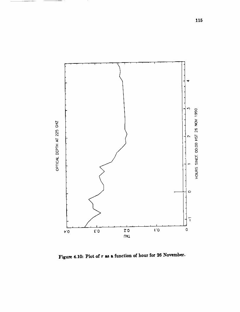
115

NI(.9

t_

C_

I

ft.t._C_

..J

_.)m

fl_O

_'0 £'0 _'0 L'O

nvi

0

I

0

Figure 4.10: Plot of r as a function of hour for 26 November.

116

Then, T_ can be written as

rhTry-, - Ca] _'7" (4.23)

Because the quantity _-y is not known, the computer gives the system temperature

as

ThT_.- Ca-'-']" (4.24)

The system temperature for each scan is listed in Tables 4.1-4.3.

We were unable to observe on the first scheduled night of observation (24

November) due to poor weather conditions (low lying cumulus cloud and fog). We

utilized this night by familiarizing ourselves with the receiver tuning process. The

zenith optical depth (r,) was stable at 0.05 on 25 November for appraximately

three hours. As the night progressed, the humidity rose from an initial 20% to

100% at around 04:00 local time. At this time, fog was visible and observations

were terminated. On 26 November, r, was higher but relatively stable at 0.2 for

appr_imately four hours. The humidity was initially high (80%) and rose to 100%

at 05:00. Fog was again visible, and we noted ice on the surface of the telescope

at this time.

4.5 Data Analysis

Using the data analysis package CLASS, we fit a zero order baseline to the observed

spectrum of each scan. The antenna temperature (T_) corrected for atmospheric

opacity is averaged over the 1024 channels of the AOS to reflect a mean and RMS

deviation for in each scan. Tables 4.1-4.3 list T_, the RMS noise, the system

temperature (T,y,), and the zenith optical depth (r) for each scan. Also listed is

the position of the antenna at the beginning of the scan (ON or OFF source). We

also note when the antenna was repositioned.

The overall observational uncertainty was dominated by scatter in the means

of individual scans and not the base line ripple observed in a single scan. As

117

Table 4.1: Listing of observations (UT) 25 November 1990 at 216 GHz.

Scan Source T_ (K) RMS (K) T.s. • ON/OFF Comments

1001 Ca] Not pointed1002 Ca]1003 Marl 47.5 3.1 ON1004 CaJ1005 Man 43.2 1.5 OFF

1006 Cal1007 Orion1008 Ca]1009 Orion1010 Ca]I011 Orion1012 Ca]

1013 Ca]1014 Ca]1015 Mars 59.4 1.5 _3.2 0.0515 OFF1016 Ca]lO1T Mars 58.4 1.4 059.2 o.or_ ONIO16 Ca/1019 Mars 59.4 1.$ 963.2 0.055 OFF1020 Ca]1021 ]vim 55.7 1.3 970.2 0.0SS ON1022 Ca]1025 Mm 59.$ 1.4 966.7 o.or_ OFF1024 Ca]

1025 Mm 60.4 1.2 980.6 0.055 ON1026 Ca]

1027 Mars 59.5 1.7 976.0 0.056 OFF1028 Ca]1029 Mars 60.$ 1.6 984.0 o.or_ OFF1030 Ca]1031 Ca]1032 Ca]1033 Ca]1034 Ca]

1035 Jupiter 162,8 2.7 1013 0.065 ON1036 Ca]

1037 Jupiter 148.2 $.5 1013 0.or_ OFF1038 C_l

1059 Jupiter 169.1 1.9 991.$ 0.0_ ON1040 Ca]

1041 Jupiter 149,9 2.9 996.5 o.or_ OFF1042 Cal

1045 Jupiter 162_ 2.2 996.1 0.0_ OFF1044 Ca]

1045 Jupiter 146.7 $.1 986.1 0.058 ON1041 Ca]1048 Man 57.8 0.5 9_2.5 o.or_ ON

1049 Cai1050 Man 62.0 0.9 91,1,.8 0.058 ON1031 Ca]1052 Man 61.1 0.9 074.$ 0.055 OFF1053 Ca]

1054 Mm 61.1' 1.1 _&0 O.OSS OFF1055 Csl•1056 Man, 57.5 0.9 _9.$ 0.055 OFF

2 Five-points

1 Five-point

$ Five-points

1 Five-point

I Fiw-polnt

I Five-po/nt

1 Five-point

118

Table 4.2: Listing of observations (UT) 26 November 1990 at 230 GHz.

sc_, Sou_. r_ (K) aMS (K) r.,. • ON/OFF Con_ent,

1001 Cal Noisy1002 Mm 47.5 $.1 ON n_k retunlngIOOS Old

1004 Mm 45.2 1.5 OFF1005 Cal1006 Mm 40.8 0.6 ON1007 Cal10045 Mm 49.2 1.5 OFF1009 Cal1010 Mm 64.$ 4.5 1348 0.213 ONI011 Cad1012 Mmm 54.6 3.1 1341 0.213 OFF1015 Cal

1014 Mmm 55.5 2.2 1947 0.213 ON1015 Cal1016 Man 54.7 2.0 15._ 0.190 OFF1017 Cal

1018 Man 55.8 2.2 IS,_2 0.190 ON1019 Cad1020 Mm 55.8 2.0 1844 0.190 OFF1021 CLI

1022 Mm 64.2 2.0 1549 0.201 ON1025 Cal1024 Man 54.0 |.1 ISM 0.201 OFF1025 Cad1026 Cal

1027 Cal1028 Jupiter 140.0 4.9 1557 0.202 OFF1029 Cal

1030 Jupiter 170_ 2.6 1492 0.202 ON1031 CIl1032 Jupiter 142.7 5.5 1521 0.202 OFFI0_ Cal

1034 Jupiter 170.9 2.6 1464 0.202 ONlOSS Cal1056 Jupiter 14S.6 5.$ 1477 0.202 OFF10S7 Ca]I0_ Jupiter 145.$ 4.7 1464 0.201 OFF1039 Cad

1040 Jupiter 166.1 2.6 1458 0.201 ON1041 Cad1042 Mm 66.0 2.6 1441 0.201 ON1045 CL!1044 Mm 66.0 2.7 1446 0.201 ON1045 Cal1046 Man 63.8 1.8 1451 0.201 OFF

1047 Cs]1048 Mm 64.$ 1.$ 14_ 0.201 OFF1049 CadlOS0 Man 63.6 1.2 1461 0.I01 OFF1051 Cad

1052 Mm 60.9 l_q 1464 0._01 ONlOr_ Cad1054 Mars 61.0 1.4 1474 0o201 OFF1055 Cal1056 Mm 63.4 2.5 1473 0._01 ON

Retuned

not pointed

2 Five-points

i Fiw,-point

2 Five-points

2 Five-points

1 Fiw-point

1 Five-point

1 Fivo-point

1 Five-point

2 Fiw,-points

1 Fiw,-point

1 Fiw,-point

119

Table 4.3: Listing of observations (UT) 26 November 1990 at 216 GHz.

Scan Source T,_ (K) RMS (K) T.,, r ON/OFF Comments

1057

1058

1059

1060

1061

1062

1063

1064

1065

1066

1067

1068

1069

1070

1071

1072

1073

1075

1076

10771078

1079

1080

1081

1082

1083

1084

1085

1086

1087

1088

1089

1090

1091

1092

1093

Ca] 1 five pointMars 47.5 0.8 1512 0.226 ON

Ca]

Mars 43.2 0.7 1540 0.224 OFF

Ca]

Mars 40.8 0.9 1559 0.224 ON

Ca]

Mars 49.2 1.5 1591 0.224 OFF

Ca] 2 Five-points

Jupiter 129.9 2.2 1093 0.224 OFFCa]

Jupiter 144.0 2.8 1113 0.230 ON

Ca] 2 Five-point

Jupiter 132.5 2.2 1113 0.236 OFF

Ca] 2 Five-points

Jupiter 147.0 2.4 1117 0.236 ON

Ca] 2 Five-pointCa]

Ca]

Orion

Ca]

Orion

Ca]

Orion

Ca]

Orion

Ca] 1 Five-point

Jupiter 147.7 1.7 1079 0.221 ONCa/

Jupiter 137.3 3.4 1083 0.218 OFF

Ca] 1 Five-point

Jupiter 147.4 1.9 1077 0.218 ONCal

Jupiter 139.3 3.1 1082 0.219 OFF

Ca] 1 Five-point

Jupiter 151.5 1.7 1085 0.219 ON

120

expected, we are limited by sky noise and systematic errors, not the sensitivity

of the receiver. The averaged observed temperatures, T_, are listed in Table 4.4.

We also list the computed values of _-y. The expected value of _'_ at 230 GHz is

apprc0cimate]y 0.72. We note that our observed vaJues of _-/varied from night to

night by as much as 10%.

The spectra of both Jupiter and Mars at the two observed frequencies are

expected to be fiat over band width (500 MrHz) of the receiver. Both random and

systematic processes contribute to the observed baseline ripple (see Figure 4.8).

The ripple is still present after averaging several scans. Therefore, it must be

systematic in part.

We aiso note systematic variations in the scans of both Jupiter and Mars.

The recorded temperatures of Jupiter from scans which began with the telescope

ON the planet were consistently higher than those from scans which began with the

telescope OFF the planet (on the sky). We believe that the computer-controlled

attenuators were not set to adequate levels on the scans which began OFF the

source. This would cause the amplifiers to be driven into compression which would

result in lower observed antenna temperatures. Compression of the amplifiers was

also observed and confirmed independent]y by Schinckel (private communication,

1991). Therefore, we believe that only the scans which started ON Jupiter are reli-

able and include only these scans in our calculation of Jupiter's observed brightness

temperatures. We list the c]ata used to derive brightness temperatures for Jupiter

at 215 and 230 GHz in Table 4.5. The uncertainty in the relative brightness tem-

peratures of Jupiter, Tj_t_r, for individuaJ nights is the quadratic sum of the

observed uncertainties in T_ for Mars and Jupiter (note: This does not include

the additional +10% uncertainty in the absolute temperature of Mars).

Our observed brightness temperatures of Jupiter and those of previous ob-

servations near 1.4 mm are reported in Table 4.6. The first uncertainty represents

the 1or statistical uncertainty in the Mars/Jupiter ratio appropriate for searching

121

Table 4.4: Observed antenna temperatures.

Freq.

(GH,)

Date

(UT)

Source T_ 4- la _.y Comments

(K)

215.31

215.31

215.31

215.31

229.60

229.60

11/25/90

11/25/90

11/26/90

11/26/90

11/26/90

11/26/90

Mars 59.7-t-0.4 0.825

Jupiter 154.9-i6.7

161.6±1.2

148.2+0.9

Mars 51.4=t=0.6 0.713

Jupiter 141.8£=6.4

147.5-1-1.2

134.7±2.5

Mars 60.5±4.4 0.743

54.810.4 0.673

63.6±0.7 0.782

Jupiter 154.5_12.9

169.2-4-1.5

143.4.-1=1.3

All scans (2 sets)

sc_(1 set)

scans starting ON source only

scans starting OFF source only

All scans (1 set)

All scans (2 sets)

scans starting ON source only

scans starting OFF source only

All scans (2 sets)

Low's only

High's only

All scans (1 set)

scans starting ON source only

scans starting OFF source only

122

Table 4.5: Observational data used to computed Jupiter's brightness temperature.

Freq. Date T_ ± la T_ -4- lo TM.,, T.ru_te,

(GHz) (UT) Mars Jupiter assumed observed

215.31 11/25/90 59.7-4-0.4 161.6,4,1.2 211.9 166.3 + 1.7

215.31 11/26/90 51.4,4,0.6 147.5,4,1.2 211.9 175.0 + 2.5

229.60 11/26/90 60.5-4-4.4 169.2+1.5 212.6 178.1 -4- 13.0

229.60 11/26/90 54.8+0.4 169.2,4,1.5 212.6 196.7 -4- 2.3

229.60 11/26/90 63.6-4-0.7 169.2+1.5 212.6 169.4 + 2.4

for possible spectral features. The second uncertainty includes an additional 10_

uncertainty in the assumed brightness temperature of Mars required for abaolute

brightness temperature measurements. Our observed brightness temperatures are

in good agreement with previous observations at wavelengths near 1.4 mm (Rather

eta/., 1974, Courtin et a/., 1977, Ulich eta/., 1984 and Gri_n eta/., 1986). All

of the previous observations were made with broadband filters (see also Table 3.3)

and only the observations of Courtin et a/. (1977) and Grit_n cta/. (1985) used

Mars as a calibrator. Rather eta/. (1974) and Ulich et a/. (1984) somewhat arbi-

trarily assigned brightness temperatures of 150 and 165 K, respectively, to Jupiter

based on their observations of several planets and previously observed planetary

brightness temperatures at longer and shorter wavelengths.

Finally, we chose to utilize the spectral information available in the 1024

channels of the AOS to obtain additional calibration information and to check for

the unlikely presence of narrow line core emission from H2S in Jupiter's strato-

sphere. We observed line emission from the core of the Orion molecular cloud on

123

Table 4.6: Observed Jovian brightness temperatures near 1.4 mm.

Wavelength Freq _ Calibrator A_

(nun) (GHz) (K) (GHz)

Reference

1.30 231 175.0±2.5(1S) Mars 3.2 This work

1.32 227 170.9+3.9(18) Mars 70 Griffin et 6L(1986)

1.32 227 165+8(18) planets 39 Ulich et 6/.(1984)

1.39 216 178.114-13.0(22) Mars 3.2 This work

1.40 214 1484-16(22) b planets 275 Rather e_ a.(1975)

1.40 214 168_II(20) c Mars 210 Courtin e_ a.(1977)

"First uncertainty is l_r observational uncertainty,

the second uncertainty includes an additional 10_ for absolute calibration

bBrightness temperatures as corrected in Berge and Gulkis (1976)

c Recalculated using beam correction factor in Ulich (1980)

124

both nights at 215.3 GHz in addition to the two planets. The hydrogen sulfide line

emission from Orion at 216.7 GHz (centered in the upper side band) was clearly

visible after one scan. If an H=S emission core is present in the scans of Jupiter,

it will also appear in the center of the upper side band. An H2S mixing ratio of

close to 1 × 10 -6 would have to be present in the stratosphere in order to detect

an emission core. Based on the strict upper limits (as low as I × 10 -_) which

have been placed on the abundance of H2S in Jupiter's stratosphere at several

wavelengths from the infrared to uv (summarized by Larson eta/., 1984), no such

feature is expected. Figure 4.11 shows an average of all scans of Jupiter at 215.3

GHz for 25 November. Indeed, no H=S emission core is visible.

The line intensities in the spectra of Orion also provide a secondary calibra-

tion source. An averaged spectrum of Orion observed on 26 November is shown in

Figure 4.12. There is good agreement between our spectra of Orion (26 November)

and those of Sutton et a/. (1985). However, the line intensities of the averaged

spectra taken on 25 November are significantly higher than those of Sutton eta/.

(1985) which could be due to a side band ratio _ 1. This might also explain the

high value of _-y observed on 25 November. Therefore, we believe the 215.3 GHz

observation on 26 November to be more reliable than the 25 November observation.

4.6 Observational Results

Figure 4.13 shows several synthetic emission spectra of Jupiter near 216 GHz using

the radiative transfer and thermochemica] model described in Chapter 3. We have

computed the Jupiter's emission using _he NH3 and HzS vertical distributions

shown in Figure 3.9. Our observed brightness temperatures and corresponding

error bars are also shown along with several other previous observations.

We were unable to obtain repeatable observations at individual frequencies

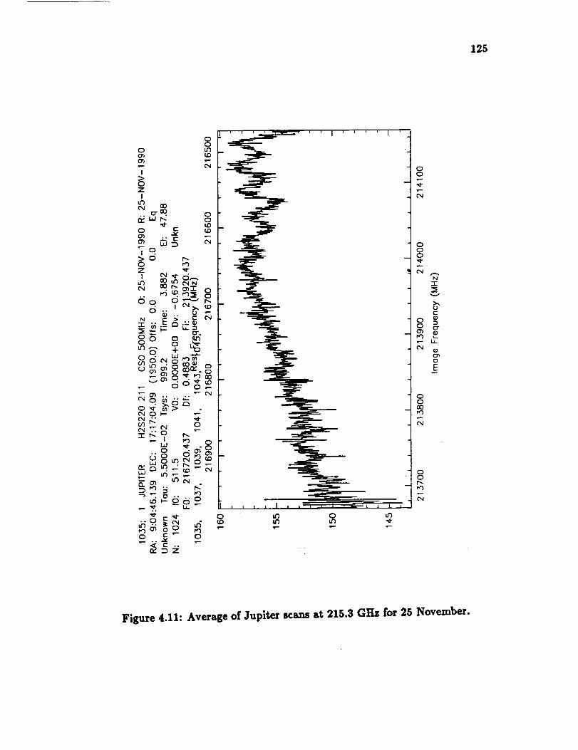
125

00

F_

000

N

-r

0E

00OO

0

Figure 4.11: Average of .Jupiter scans at 215.3 GHz for 25 November.

126

i i i I i

(,/I

i

,q-

(M

Figure 4.12: Average of Orion scans at 215.3 GHz for 26 November.

127

205

2OO

_, 195

r_ 190

185

IE(I,:_ 180Iup,

u_ 175r_Z[-=: 170i--!

165

16020(

Jupiter's observed and computed spectrum near 1.4 mm

; : i I i i i

NH3 2 no H2S

........ --. NH., 2 ._--" :"-..... +, .o.....H2S i

+, +,,i i f, I II I ' ¢, I

i !_ NH3, 1 !no,H2S J

H2S

this:this: work:wo rkm !Z I

i , i/i, , ,i , 1 , 1,

205 210 215 220 225 230

|

235 240

FREQUENCY (CHz)

Figure 4.13: Observed spectrum of Jupiter near 216 GHz. e: our observations;

o: other observations from Table 4.6. Theoretical spectra using distributions in

Figure 3.9, sol|d ILue: NHa, HsO, and pressure-induced opacity only; dashed line:

H=S opacity added.

128

over several nights due to poor weather conditions. The uncertainties for our ob-

servation (especially for the single observation at 229.6 GHz) are large. Therefore,

we did not detect a statistically significant difference in emission due to H_S at

the two wavelengths. Although we were unable to set tighter limits on the H_S

abundance in Jupiter's atmosphere, our results reinforce previous limits summa-

rized by Larson et _., 1985. Even though we did not achieve our primary objective

of detectLug H_S gas, we Were able to measure Jupiter's brightness temperature

relative to Mars at the highest spectral resolution recorded at this wavelength.

129

CHAPTER 5

Summary and Conclusion

5.1 Uniqueness of Work

This research makes contributions in the areas of both planetary science and

millimeter-wave measurements. The major contributions are summarized below:

1. Conducted first laboratory measurements of gaseous NHs opacity at Ka-band

(v = 32 - 40 GHz, _ = 7.5 - 9.38 ram) under simulated Jovian conditions

2. Conducted first laboratory measurements of gaseous NHs opacity at W-band

(v = 94 GHz _ = 3.2 ram) under simulated Jovian conditions

3. Developed new parameterization of the Ben-Reuven line shape for computing

the absorptivity of NHs under Jovian conditions

4. Conducted first laboratory measurement of the hydrogen and helium broad-

ened line width of gaseous H=S at 1.4 mm

5. Documented for the first time new techniques in millimeter-wave measure-

ments (e.g., laser tuning of the resonator) and documented for the first time

solutions to problems which occur in millimeter-wave measurements (e.g.,

dielectric loading)

6. Incorporated for the first time the results of the millimeter-wave laboratory

absorption measurements of NHs and H=S into a radiative transfer model

and computed synthetic emission spectra from the four giant planets

130

7. Developed new expressions for computing the radio opacity of pressure_

induced absorption from Hz-H2, H2-He and H2-CH4 pairs and water vapor

under Jovian conditions

8. Demonstrated that Jupiter's observed millimeter-wave emission is entirely

consistent with synthetic spectra in which NHs is the primary source of

opacity

9. Observed Jupiter at 1.4 mm for the first time using a high resolution receiver

and obtained a reliable brightness temperature of Jupiter using Mars as the

calibration standard

This research has culminated in the publication of several journal papers:

Joiner et a/. (1989), Joiner and Steffes (1991), and Joiner et a/. (1991). This

research has also been presented as several conference reports: Joiner eta/. (1987),

Joiner and Steffes (1988), Joiner and Steffes (1989), Joiner and Steffes (1990a,b).

5.2 Suggestions for Future Research

Although we were unable to obtain a positive detection or H2S or set new up-

per limits on the H_S abundance in Jupiter's atmosphere, the search for H2S at

millimeter wavelengths should not be abandoned. Poor weather conditions and in-

strumental difliculties contributed to large uncertainties in our observation. How-

ever, given more ideal conditions, the statistical uncertainties could be significantly

reduced and systematic effects eliminated. In order to reduce the observational

uncertainty, the integration time must be increased (i.e., observations should be

repeated over several days). Weather conditions must be exceptional in order to

eliminate any variations in the observed temperatures of Jupiter and Mars caused

by variations in the earth's atmospheric opacity. In addition, observations should

be made at a minimum of three frequencies, corresponding to the center of the

131

H2S line and on both sides of the line, in order to achieve a convincing detect|on

of the pressure-broadened line.

Improvements in millimeter-wave technology will make the detection of broad

spectral features (i.e., pressure-broadened lines in planetary atmospheres) more

feasible in the future. Wide band oscillators coupled with computer-controlled

tuning will significantly reduce the time required to tune receivers. In addition,

new instruments which can be mounted on existing millimeter and submiIlimeter

antennas, such as Fourier Transform Spectrometers, will be better suited for the

detection of broad spectral features. In the future, spectrometers with the proper

resolution (on the order of GHz) for planetary spectroscopy will be utilized to

improve upon the results obtained with the multi-wavelength approach. Improved

calibration techniques will reduce the large uncertainty that presently exists in the

absolute calibration of millimeter planetary observations.

Although this research represents great strides in the understanding of the

millimeter-wave spectra of the Jovian planets, more microwave and millimeter-

wave laboratory measurements are needed in order to fully interpret all of the

available planetary observations. For example, measurements of the millimeter

dielectric properties of solid NHa and NH4SH are needed to accurately assess

the potential effect of cloud condensates on the millimeter-wave spectra of the

giant planets. Absorption measurements of pressure-broadened H2S at centimeter

wavelengths are needed in order to interpret the centimeter emission from Uranus

and Neptune. In addition, a measurement of the equilibrium constant for the

reaction of NH3 and H2S to form solid NH4SH is needed in order to accurately

predict the altitude at which the putative NH4SH cloud will form. It is hoped that

this research has provided the initiative for continued exploration of the millimeter-

wave spectrum as part of the study of the Jovian planets.

132

BIBLIOGRAPHY

ASTRONOMICAL ALMANAC 1990. U. S. Naval Observatory, U. S. Govt. Print-

Lug Office,Washington, D. C.

ANDERS, E. AND N. GREVESSE 1989. Abundances of the elements: mete-

oriticand solar. Geochim. Cosmochim. Aeta 53, 197-214.

ATREYA, S. K.AND P. N. ROMANI 1985. Photochemistry and clouds of

Jupiter, Saturn, and Uranus. In R_cent advances in planetary meteorology.

ed. G. E. Hunt. Cambridge Univ. Press, Cambridge, 17-68.

BAARS, J. W. M., R. GENZEL, I. I. PAULINY-TOTH, AND A. WITZEL

19 77. The absolute spectrum of Cas A: an accurate flux density scale and

a set of secondary calibrators.Astron. Astrophys. 61, 99-106.

BACHET, G., E. R. COHEN, P. DORE, AND G. BIRNBAUM 1983. The

translational-rotationalabsorption spectrum of hydrogen. Can. J. Phys 61,

591-603.

BATTAN, L. J. 1973. Radar Observation of the Atmosphere. University of

Chicago Press, Chicago.

BEN-REUVEN, A. 1966. Impact broadenLug of microwave spectra. Phys. Rev.

145, 7-22.

BERGE, G. L., AND S. GULKIS 1976. Earth-based radio observation of

Jupiter: Millimeter to meter wavelengths. In Jupiter (T. Gehrels, Ed.), 621-

692. Univ. of Arizona Press, Tuscon.

BEZARD, B., A. MARTEN, J. P. BALUTEAU, D. GAUTIER, J. M. FLAUD,

AND C. CAMY-PEYRET 1983. On the detectabilityof H2S in Jupiter.

lmru_ 55,259-271.

BJORAKER, G. L., H. P.LARSON, AND V. G. KUNDE 1986A. The gas

composition of Jupiter derived from 5 #m airborne spectroscopic observa-

tions. Icarus 66, 579-609.

BJORAKER, G. L., H. P.LARSON, AND V. G. KUNDE 1986B. The abun-

dance and distributionof water vapor in Jupiter'satmosphere Astrophys. J.

811, 1058-1072.

133

BORYSOW, J., L. TRAFTON, AND L. FROM]VIHOLD 1985. Modeling of

Pressure-Induced Far-Infrared Absorption Spectra: Molecular Hydrogen Pairs.

Aatrophys. J. 296, 644-654.

BRIGGS, F. H., AND P. D. SACKETT 1989. Radio observations of Saturn

as a probe of its atmosphere and cloud structure. Icarus 80, 77-103.

CRC PRESS 1983. CRC Handbook of Chemistry and Physics (R. C. Weast,

Ed.). CRC Press, Boca Raton, FL.

CHEDIN, A., N. HUSSON, N. A. SCOTT, I. COHEN HELLALET, A. BERROIR

1982. GEISA data bank (No 3).

COGDELL, J. R., J. H. DAVIS, B. T. ULRICH, AND B. J. WILLS 1975.

Flux density measurements of radio sources at 2.14 millimeter wavelength.

Astrophys. J. 196, 363-368.

COLLIN, R. E. 1966. Foundations for Microwave Engineering. McGraw-Hill,

New York.

COURTm, R., N. CORON, T. ENCRENAZ, R. GISPERT, P. BRUSTON,

J. LEBLANC, G. DAMBIER, A. VIDAL-MADJAR 1977. Observations

of giant planets at 1.4 mm and consequences on the effective temperatures.

Astron. Astrophlts. 60, 115-123.

DEPATER, I., AND S. T. MASSIE 1985. Models of the millimeter-centimeter

spectra of the giant planets. Icarus 62, 143-171.

DEPATER, I. 1986. Jupiter's Zone Belt Structure at Radio Wavelengths: H.

Comparison of Observations with Atmosphere Calculations. Icarus 68, 344-

365.

DEPATER, I., P. N. ROMANI AND S. K. ATREYA 1989. Uranus deep

atmosphere revealed. Icarus 82, 288-313.

DEPATER, I., P. N. ROMANI AND S. K. ATREYA 1991. Possible microwave

absorption by H2S gas in Uranus' and Neptune's atmospheres. Icarus 91,

220-233.

DEPATER, I. AND M. RICHMOND 1989. Neptune's microwave spectrum from

1 mm to 20 cm. Icarus 80, 1-13.

DEIRMENDJIAN, D. 1969. Electromagnetic Scattering on Spherical Polltdis-

persions, American Elsevier Publishing Co, Inc., New York.

134

DORE, P., L. NENCINI, AND G. BIRNBAUM 1983. Far infrared absorption

in normal H2from 77 to 298 K. J. Quant. Spec. Rad. Trans 30, 245-253.

FLAUD, J. M., C. CAMY-PEYRET, AND J. W. C. JOHNS 1983. The far

infrared spectrum of hydrogen sulfide. Can. J. Phys. 61, 1462-1473.

GAGLIARDI, R. M. 1084. Satellite Communications, Lifetime Learning Pub-

lications, Wadsworth, Inc., Belmont, CA.

GASIEWSKI, A. J. 1990. Microwave radiative transfer in hydrometers. In

Atmospheric Remote Sensing by Microwave Radiometry (M. A. Jxnssen, ed.)

To be published by John Wiley and sons.

GAUT N. E. AND E. C. REIFENSTEIN III 1971. Environmental Research

and Technology, Inc.,Report No. 13, Lexington, MA.

GOODMAN, G. C. 1969. Models of JupRer's atmosphere Ph. D. thesis,Uni-

versityof Illinois,Urbana.

GRIFFIN, M. J., P. A. R. ADE, G. S. ORTON, E. I. ROBSON, W. K.

GEAR, I. G. NOLT, AND J. V. RADOSTITZ 1986. SubmUlimeter and

millimeter observations of Jupiter. Icarus 65,244-256.

GROSS, E. P. 1955. Shape of collision-broadenedspectral lines.Phys. Rev.

97, 395-403.

GROSSMAN, A. W. 1990. Microwave imaging of Saturn's deep atmosphere

and rings. Ph.D. thesis,California Instituteof Technology, Pasadena.

GULKIS, S. 1987. Radio astronomy, planetary. Encycl. Phys. Sci. Tech., Vol.

II, 633-654.

GULKIS, S. AND I. DEPATER 1984. A review of the millimeter and centimeter

observations of Uranus. In Uranus and Neptune: Pro¢. of a work.shop held

in P_sadena, CA, Feb. 6-8, I#8J, NASA Conf. Publ. 2330, 225-262.

HELMINGER, P. AND F. C. DELUCIA 1972. Pressure broadening of hydrogen

sulfide. J. Quant. Spectrose. Rad. Trans. IT, 751-754.

HOFSTADTER, M. D., G. L. BERGE AND D. O. MUHLEMAN 1990.

Vertical motions in the Uranian atmosphere: an analysis of radio observation.

Icarus S4, 261-267.

135

HOFSTADTER, S. D. AND D. O. MUHLEMAN 1988. Latitudinal varia-

tions of ammonia in the atmosphere of Uranus: an analysis of microwave

observations. Icarus 81, 396412.

JOINER, J., JENKINS, J. M., AND STEFFES, P. S., (1987). Laboratory

Measurements of the Opacity of Gaseous Ammonia (NHs) in the 7.3 - 8.3 mm

(36-41 GHz) Range Under Simulated Conditions for the Jovian Atmospheres,

Bull. Amer. Aatron. Soc. 19, 838.

JOINER, J., JENKINS, J. M., AND STEFFES, P. S., (1988). Millimeter-wave

Measurements of the Opacity of Gaseous Ammonia (NHs) Under Simulated

Conditions for the Jovian Atmospheres, Bull. Amer. Astron. Soc. 20, 867.

JOINER, J., P. G. STEFFES, AND J. M. JENKINS 1989. Laboratory

measurements of the 7.5-9.38 mm absorption of gaseous ammonia (NHs)

under simulated Jovian conditions. Icarus 81, 386-395.

JOINER, J., AND STEFFES, P. G. (1989). Models of the Millimeter-wave

Emission of the Jovian Atmosphere Utilizing Laboratory Measurements of

Gaseous Ammonia (NHs). Bull. Amer. Astron. Soe. 21, 945.

JOINER, J., AND STEFFES, P. G. (1990). Study of the Millimeter-wave Ab-

sorbing Constituents in the Jovian Atmospheres. Bull. Amer. Astron. Soc.

22, 1032.

JOINER, J., AND STEFFES, P. G. (1990). Measurement of the Pressure-

Broadened Linewidths of Gaseous Hydrogen Sulfide (H_S). Poster presented

at Second International Conference on Laboratory Research for Planetary

Atmospheres.

JOINER, J., AND P. G. STEFFES 1990. Modeling of Jupiter's mUlimeter-

wave emission utilizing laboratory measurements of ammonia (NHs) opacity.

JGR:Pianets, accepted.

JOINER, J., P. G. STEFFES, AND K. S. NOLL 1990. Search for sulfur

(H2S) on Jupiter at millimeter wavelengths. Submitted to IEEE Trans. Mi-

crowave Theor. Teeh.

KLEIN, M, J. AND S. GULKIS 1978. Jupiter's atmosphere: Observations and

interpretation of the microwave spectrum near 1.25 cm wavelength. Icarus

35, 44-60.

136

KLEIN, M. J., M. A. JANSSEN, S. GULKIS AND E. T. OLSEN 1978.

Saturn's microwave spectrum: Implications for the atmosphere and the rings.

In The Saturn System, NASA CF-2068, (D. M. Hunten and D. Morrison,

Eds.), 195-216. NASA, Washington, D. C.

KRAUS, G. F., J. E. ALLEN, JR., AND L. C. COOK 1989. Vapor

pressure measurements of hydrogen sulfide. Bull. Amer. Astro,. Soc. 21

948.

LARSON, H. P., D. S. DAVIS, R. HOFMAN, AND G. L. BJORAKER

1984. The Jovian atmospheric window at 2.7 microns: A search for H2S.

Icarus 60, 621-639.

LELLOUCH, E., T. ENCRENAZ AND F. COMBES 1984A. The observabilityof

HCN on Jupiter in the millimeter range. Astron. Astrophys. 185,365-370.

LELLOUCH, T. ENCRENAZ AND E., F. COMBES AND P. DROSSART 1984B.

The observability of HCN and PHs on Saturn in the millimeter range. As-

iron. Astrophl/s. 135, 371-376.

LELLOUCH, E., F. COMBES, AND T. ENCRENAZ 1984c. Microwave observa-

tions of Jupiter and Saturn. Astron. Astrophvs. 140, 216-219.

LELLOUCH, E., J. L. DESTOMBES 1985. Search for minor atmospheric

species in the millimeter range of Jupiter and Saturn. Astron. Astrophlls.

152, 405-412.

LINDAL, G. F., G. E. WOOD, G. S. LEVY, J. O. ANDERSON, D. N.

SWEETNAM, H. B. HOTZ, B. J. BUCKLES, D. P. HOLMES, P. E.

DAMS, V. R. ESHLEMAN, G. L. TYLER, AND T. A. CROFT 1981.

The atmosphere of Jupiter: An analysis of the Voyager Radio Occultation

measurements..I. Geophvs. Res. 86, 8721-8727.

LINDAL, G. F., D. N. SWEETNAM, AND V. R. ESHLEMAN 1985. The

atmosphere of Saturn: An analysis of the Voyager Radio Occultation mea-

surements. J. Geophl/s. Res. 90, 1136-1146.

LINDAL, G. F., J. R. LYONS, D. N. SWEETNAM, V. R. ESHLEMAN,

D. P. HINSON, AND G. L. TYLER 1987. The atmosphere of Uranus An

analysis of the Voyager Radio Occultation measurements. J. Geophys. Res.

93, 14987-15002.

MIE, G. 1908. Beitrage zur optik truber medien, speziell kol]oidaler metala-

sungen. Ann. Physik, 35,377.

137

MORRIS, E. C., AND R. W. PARSONS 1970. Microwave absorption by gas

mixtures at pressures up to several hundred bars. Astron. J. Phys. 23,

335-349.

PHILLIPS, T. G. 1989 Caltech Submillimeter Observatory (CSO) Handbook.

PALTRIDGE, G. W. AND C. M. R. PLATT 1976. Radiative Processes in

Metwrology and Climatologl/,American Elsevier Publishing Co., Inc.,New

York.

POLLACK, J. B., AND P. BODENHEIMER 1989. Theories of the origin

and evolution of the giant planets. In Origin and evolution o� atrnospherea

(S. K. Atreya, J. B. Pollack and M. S. Matthews, Eds.), 564-602.

POYNTER, R. L., AND R. K. KAKAR 1975. The microwave frequencies,

line parameters, and spectral constants for NHs. Astrophlla. J. Suppl. 29,

87-96.

RATHER, J. D. G., B. L. ULICH, AND P. A. R. ADE 1974. Planetary

brightness temperature measurements at 1.4 mm wavelength. Icarus 23,

448-453.

ROMANI, P. N., I. DEPATER, AND S. K. ATREYA 1989. Neptune's deep

atmosphere revealed. Geophvs. Rea. Left. 16, 933-936.

RUDY, D. J., D. O. MUHLMENAM, G. L. BERGE, B. M. JAKOSKY,

P. R. CHRISTENSEN 1987. Mars: VLA observations of the northern

hemisphere and the northern polar region at wavelengths of 2 and 6 cm.

Icarus YI, 159-177.

SILL, G., U. FINK, AND J. R. FERRARO 1980. Absorption coefficients of

solid NHs from 50-7000 cm -l. J. Opt. Soc. Arr_ TO, 724-739.

SPILKER, T. R. 1990. Laboratory measurements of Microwave absorptivity

and refractivity spectra of gas mixtures applicable to giant planet atmo-

spheres. Ph. D. thesis, Stanford University, Stanford.

STEFFES, P. G., AND J. M. JENKINS 1987. Laboratory measurements of

the microwave opacity of gaseous ammonia under simulated conditions for

the Jovian atmosphere. Icarus '/B, 35-47.

SUTTON, E. C., G. A. BLAKE, C. R. MASSON, AND T. G. PHILLIPS

1985. Molecular line survey of Orion A from 215 to 247 GHz. Astrophlls.

J. Suppl. 58, 341-378.

138

TERMAN, F. E. 1043. Radio Engineera' Handbook. McGraw-Hill Book Com-

pany, Inc., New York.

TOWNES, C. H., AND A. L. SHAWLOW 1955. Microwave Spectroscopy.

McGraw-Hill, New York.

TYLER,G. L., D. N. SWEETNAM, J. D. ANDERSON, S. E. BORUTZKI,

J. K. CAMPBELL, V. R. ESHLEMAN, D. L. GRESH, E. M. GUR-

ROLA, D. P. HINSON, N. KAWASHIMA, E. R. KURSINSKI, G. S. LEVY,

G. F. LINDAL, J. R. LYONS, E. A. MAROUF, P. A. ROSEN,

R. A. SIMPSON, AND G. E. WOOD 1989. Voyager radio science obser-

vations of Neptune and Triton. Science 86, 1466-1473.

ULABY, F. T., R. K. MOORE, A. K. FUNG 1981. Microwave Re-

mote Sensing Active and Passive. Addison-Wesley Publishing Company,

Inc., Reading, MA.

ULICH, B. L. 1974. Absolute brightness temperature measurements at 2.1

mm wavelength. Icarus 21, 254-261.

ULICH, B. L. 1981. Millimeter, wavelength continuum calibration sources.

Astron. J. 86, 1619-1626.

ULICH, B. L., J. R. COGDELL, AND J. H. DAWS 1973. Planetary

brightness temperature measurements at 8.6ram and 3.1 mm wavelengths.

I_rus 19, 59-82.

ULICH, B. L., J. H. DAVIS, P. J. RHODES, AND J. M. HOLLIS

1980. Absolute brightness temperature measurements at 3.5 mm wave-

length. IEEE Trans. Ant. Prop., AP-28, No. 3, 367-377.

ULICH, B. L., J. R. DICKEL, AND I. DEPATER 1984. Planetary Obser-

vations at a wavelength of 1.32 ram. Icarus 60, 590-598.

VALKENBURG, E. P. AND V. E. DERR 1966. A High-Q Fabry-Perot

interferometer for water vapor measurements in the 100 Gc/s to 300 Gc/s

frequency range. Proc. IEEE 54, No. 4, 493-498.

VAN VLECK, J. H., AND V. F. WEISSKOPF 1945. On the shape of

collision-broadened lines. Rev. Mod. Phys. 1Y, 433-443.

WALLACE, L. 1980. The structure of the Uranus atmosphere. Icarus 43,

231-259.

139

WATERS, J. W. 1976 Absorption and emission of microwave radiation by

atmospheric gases. In Methods of Ezperimental Physics, M. L. Meeks, ed.,

12 Part B, Radio Astronomy, Academic Press, Section 2.3.

WERNER M. W., G. NEUGEBAUER, J. R. HOUCK, AND M. G. HAUSER

1978. One millimeter brightness temperatures of the planets. Icarus SS,

289-296.

WEST R. A., D. F. STROBEL, AND M. G. TOMASKO 1986. Clouds,

aerosols, and photochemistry in the Jovian atmosphere. Icarus 65,161-217.

WEIDENSCHILLING, S. J., AND J. S. LEWIS 1973. Atmospheric and cloud

structures of the Jovian planets. Icarus 20, 465-476.

WILLEY, D. R., T. M. GOYETTE, W. L. EBENSTEIN, D. N. BITTNER,

AND F. C. DELUCIA 1989. Collisionally cooled spectroscopy: Pressure

broadening below 5K. J. Chem. Phys. 91, 122-125.

ZHARKOV, V. N. AND V. P. TRUBITSYN 1978. Physics of Planetary

Interiors (W. B. Hubbard, Ed.), vo]. 6 of Astronomy and Astrophysics Series.

Puchart Publishing House, Tucson, AZ.

ZHEVAKIN, S. A., AND A. P. NAUlVIOV 1963. Coefficient of absorption of

electromagnetic waves by water vapor in the range 10 microns-2 cm. Radio-

phys. Quantum Electron. 6, 674-694.