m-pesa and financial inclusion in kenya: of paying comes
TRANSCRIPT

HAL Id: hal-01591200https://hal.archives-ouvertes.fr/hal-01591200
Preprint submitted on 21 Sep 2017
HAL is a multi-disciplinary open accessarchive for the deposit and dissemination of sci-entific research documents, whether they are pub-lished or not. The documents may come fromteaching and research institutions in France orabroad, or from public or private research centers.
L’archive ouverte pluridisciplinaire HAL, estdestinée au dépôt et à la diffusion de documentsscientifiques de niveau recherche, publiés ou non,émanant des établissements d’enseignement et derecherche français ou étrangers, des laboratoirespublics ou privés.
M-PESA and financial inclusion in Kenya: of payingcomes saving?
Antoine Dubus, Leo van Hove
To cite this version:Antoine Dubus, Leo van Hove. M-PESA and financial inclusion in Kenya: of paying comes saving? .2017. �hal-01591200�

M-PESA and financial inclusion in Kenya: of paying comes saving?
Antoine Dubus* and Leo Van Hove
**
This version: April 26, 2017
* Télécom ParisTech, 46 rue Barrault, 75013, Paris, France, +33688910336, corresponding author,
** Department of Applied Economics (APEC), Vrije Universiteit Brussel (Free University of Brussels)
Mobile financial services are said to promote inclusion. However, only 7.6 per cent of
Kenyans have ever saved on an M-PESA account. This paper uses a novel, three-step probit
analysis to identify the socio-demographic characteristics of, successively, respondents who
do not have access to a SIM card, have access to a SIM but do not have an M-PESA account,
and, finally, have an account but do not save on it. We find that those who are left behind are
predominantly those who would benefit most from formal saving, namely the poor, the
non-educated, and, in the final step, also women.
Keywords – financial inclusion, saving, Kenya, mobile financial services, M-PESA
!

! 2
M-PESA and financial inclusion in Kenya: of paying comes saving?
Mobile financial services are said to promote inclusion. However, only 7.6 per cent of
Kenyans have ever saved on an M-PESA account. This paper uses a novel, three-step
probit analysis to identify the socio-demographic characteristics of, successively,
respondents who do not have access to a SIM card, have access to a SIM but do not have
an M-PESA account, and, finally, have an account but do not save on it. We find that those
who are left behind are predominantly those who would benefit most from formal saving,
namely the poor, the non-educated, and, in the final step, also women.
1. Introduction
Just like many other countries at a similar stage of economic development, Kenya is characterised by a
low rate of financial inclusion. Financial inclusion refers to access to financial services such as deposit,
transfer, and payment services, as well as saving, credit, and insurance. In 2014 only 55.2 per cent of
the Kenyan population over 15 had an account at a formal financial institution, compared to 93.6 per
cent in the United States (Demirgüç-Kunt & Klapper, 2014).
Informal financial systems are well developed in Kenya (Gugerty, 2007; Johnson, 2016). However, it is
commonly believed that widespread access to formal financial tools reduces poverty, stimulates
investment, and creates growth, particularly in rural areas (Morduch, 1994; Binswanger & Khandker,
1995; Beck, Demirgüç-Kunt & Levine, 2005). Especially the ability to save in a secure way would
make the difference, as it increases the resilience of the poor to income shocks and may, ultimately,
even enable them to invest in a business.
It is thus not surprising that the promotion of formal saving in developing countries is drawing the
attention of a growing research community. In this paper, we study the uptake of so-called mobile
financial services (MFS) in Kenya. MFS are said to promote financial inclusion, not only by directly
giving users access to financial services by way of their mobile phone account, but also by supposedly

! 3
functioning as a stepping stone toward the adoption of a traditional bank account 1. Kenya is a country
where MFS could have a particularly high impact, for a number of reasons. On the demand side, there
is the high level of poverty in combination with the importance of rural areas. Specifically, the high
dependence on agriculture is a vector of financial instability among rural households, which, in turn,
implies that emergency remittances – often from relatives who live in the city – are of vital importance.
On the supply side, the penetration of bank accounts is low 2, particularly in rural areas, but adoption
of M-PESA – the leading local mobile money transfer service – is widespread. In our analysis, we will
even assimilate MFS in Kenya with M-PESA, representing as it did 96 per cent of all MFS accounts in
the country in 2013 (InterMedia, 2013), and 95 per cent of the value of all MFS transfers in 2014
(Winn, 2016).
In particular, we look into which socio-demographic factors promote or inhibit saving on MFS. Unlike
existing studies, which simply compare MFS users and non-users in terms of savings (and/or
remittances), we tackle this question in three steps. We first examine which Kenyans own or have
access to a SIM card, as this is an essential precondition for being able to open an M-PESA account. In
a second step we then examine which individuals in this subsample have an M-PESA account. In a
third and final step we examine which M-PESA users actually save on their mobile phone account. In
each of these steps, we perform our analyses for three, increasingly narrow (sub)samples, namely the
full sample, the rural population, and, finally, inhabitants of rural areas who do not own a bank account
and who never send remittances. The idea is to gradually zoom in on the poorer, more vulnerable
groups in the Kenyan population. Tellingly, as we do so, all three indicators that we focus on – access
to a SIM, possession of an M-PESA account, and saving on M-PESA – progressively go down.
To improve our understanding of the behaviour of all these population segments, the paper first
analyses the body of articles on the uptake of MFS in Kenya. We highlight that the existing literature
finds different propensities to use M-PESA as a tool for saving. We show that this is due to conceptual
differences and also to the timing of the studies, a crucial factor when analysing any fast growing
technology. In the empirical part of our paper, we perform probit analysis on data taken from the
Financial Inclusion Insights Program survey conducted by InterMedia in 2013 among 3,000 !!!!!!!!!!!!!!!!!!!!!!!!!!!!!!!!!!!!!!!!!!!!!!!!!!!!!!!!!!!!!1 This is a key premise of the recent report of the CPMI-World Bank Group Task Force on the Payment
Aspects of Financial Inclusion (PAFI): “a transaction account is an essential financial service in its own right and can also serve as a gateway to other financial services” (CMPI & World Bank, 2016, p. 2).
2 Based on a nationally representative dataset collected by FinAccess Kenya in 2006 – that is, prior to the launch of M-PESA – Johnson and Nino-Zarazua (2011, p. 482) report that only 18.5 per cent of Kenyans used formal services, 8.1 per cent used semi-formal services, 35.0 per cent used the informal sector, and no less than 38.3 per cent were completely excluded. For more recent figures, see Evans and Pirchio (2014).

! 4
respondents. We find that those who are ‘left behind' are predominantly those who would benefit most
from formal saving, namely the poor, the non-educated, and, in the final step, also women. Moreover,
the problem is, by and large, bigger for the rural than for the urban population. As such, our paper
brings a sobering note to the more optimistic results of, in particular, Suri and Jack (2016), who
estimate that M-PESA has lifted 2 per cent of Kenyan households out of poverty.
The remainder of the paper is structured in six sections. Section 2 explains the concept of M-PESA as
well as its state of affairs in Kenya around the time of the data collection. Section 3 reviews the
literature. In Sections 4 and 5 we present, respectively, the survey data and our methodology. Finally,
Section 6 presents our results and Section 7 concludes.
2. M-PESA Identikit
The basic concept of MFS is simple: mobile phone airtime is transferred by way of text messages and a
network of agents working for the MFS provider allows users to withdraw money from or deposit
money into their mobile account. In Kenya, M-PESA was launched in 2007 after Safaricom, a leading
mobile services provider, had noticed that customers exchanged airtime to transfer money between
them. M-PESA formalised this practice, and the concept expanded fast, in part thanks to the high
penetration rate of mobile phones 3. By 2013, 74 per cent of the population over 15 had an account
with one of four MFS providers: M-PESA, Airtel Money, yuCash, and Orange Money (di Castri &
Gidvani, 2013).
Today, M-PESA offers multiple services (see Table 1), but, as explained, money transfers were
developed first. This service only relies on the airtime account and enables user-to-user transfers.
Transfers to non-users are also possible but incur higher charges. Nowadays the transfer option can also
be used to pay in shops. M-PESA mobile banking, for its part, comprises services similar to those
offered by traditional banks. Some of these services require a link between the user's mobile account
and a bank account. For instance, in 2010 M-PESA in partnership with Equity Bank developed
M-KESHO. M-KESHO offers a suite of financial services, such as insurance, but also an
interest-paying bank account held at Equity Bank. The interest rate ranges from 0.5 per cent to 3 per
cent, depending on the amount saved (Mbiti & Weil, 2014). M-PESA has also developed M-SHWARI, !!!!!!!!!!!!!!!!!!!!!!!!!!!!!!!!!!!!!!!!!!!!!!!!!!!!!!!!!!!!!3 In June 2015, 83.9 per cent of the population had a mobile phone subscription. In December 2007 this
number was 30.5 per cent. Data from the Communication Authority of Kenya, respectively: <http://ca.go.ke/images/downloads/STATISTICS/Sector per cent20Statistics per cent20R2015.pdf> and <http://ca.go.ke/images/downloads/STATISTICS/Sector per cent20Statistics per cent20Report per cent20Q2 per cent202008.pdf>

! 5
this time in partnership with Commercial Bank of Africa (CBA). At 5 per cent, the interest rate on an
M-SHWARI account is higher. It also provides micro-loans for a period of thirty days.
Table 1. Penetration of M-PESA uses (N = 3,000)
Number Percentage
Own a SIM card a 2459
82.0 Own or have access to a SIM card b 2836
94.6
Use M-PESA 2180 72.7 Use M-KESHO 34 1.1 Use M-SHWARI 283 9.4 Mobile money transfers
Withdraw money 2307 76.9 Deposit money 1878 62.6 Pay for goods at a store 54 1.8 Receive money for regular support 1236 41.2 Send money for regular support 1119 37.3 Receive money for emergency 763 25.4 Send money for emergency 766 25.5
Mobile banking Save money for future purchase/payment 205 6.8 Receive a salary 59 2.0 Take a loan 37 1.2 Receive state aid or pension 18 0.6 Buy insurance 5 0.2
Notes. Source: InterMedia, The Financial Inclusion Insights Program, 1. a ‘Own a SIM card’ includes 9 respondents who have a mobile phone but say they do not own a SIM card. b ‘Own or have access to a SIM card’ includes 2 respondents who have a mobile phone but say they do not own a SIM card.
Given this wide range of MFS in Kenya, how did we define MFS-enabled financial inclusion for the
purposes of our paper? Our starting point was Klapper and Singer (2014)'s broad definition of financial
inclusion as “access to and usage of appropriate, affordable, and accessible financial services”.
However, we opted for a narrow definition of ‘financial services’. We do not consider the mere use of
an M-PESA account for person-to-person transfers to be sufficient for ‘real’ financial inclusion. The
ability to receive remittances by way of M-PESA is an obvious improvement over past practices (see
Section 3), but it does leave recipients in a dependent position. In line with the old saying that we
paraphrase in the title of our paper – “Of saving comes having” – we consider the ability to save as a

! 6
necessary condition for full financial inclusion. In other words, we think that mobile payments are not
enough 4, and we therefore set out to examine to what extent ‘paying’ leads to ‘saving’ – and,
hopefully, ultimately ‘having’. From this perspective, saving on M-KESHO and M-SHWARI clearly
qualifies. But we also consider people who simply save on their mobile account as financially included,
even though such funds do not earn any interest. Demombynes and Thegeya (2012) call this “basic
mobile savings”, as opposed to “bank-integrated mobile savings”.
In the survey data that we exploit (see Section 4), the proportions of people using M-PESA for the
different operations are as listed in Table 1 5. As can be seen, basic operations such as withdrawing,
depositing, or receiving and sending money are widely used. Kenyans seem, however, less keen on the
more evolved mobile banking services, since only 6.8 per cent of the respondents had, at the time of the
survey, ever saved with M-PESA 6.
Note that MFS and banking inclusion are not exclusive. Some people own both an M-PESA and a bank
account, others own just one of the two, and some none. The main factors limiting the adoption of
formal bank accounts are distance, cost, and paperwork (Allen, Demirgüç-Kunt, Klapper, & Martinez
Peria, 2016). Conversely, M-PESA allows immediate remote transfers, it is relatively cheap, and one
only needs an ID to open an account. Even the more advanced services such as M-KESHO and
M-SHWARI retain the original spirit of M-PESA: opening an account is free and charges are relatively
low. To sign up for M-KESHO, people also do not need to go to a bank; they can do so by way of
Safaricom agents (Demombynes & Thegeya, 2012). These advantages over traditional banking would
suggest that M-PESA can indeed increase financial inclusion.
3. Related Literature
Following Donner and Tellez (2008), we discuss the relevant articles about M-PESA depending on
!!!!!!!!!!!!!!!!!!!!!!!!!!!!!!!!!!!!!!!!!!!!!!!!!!!!!!!!!!!!!4 This is in line with the PAFI Task Force mentioned earlier: “While of utmost importance, access to and usage
of a transaction account to facilitate payments and to store value is just an initial step in becoming fully financially included, which involves having access to the whole range of financial products and services that meet the user’s needs” (CPMI, 2016, p. 6). Johnson (2014, p. 3) is even more explicit: “Beyond use for payments, whether or not people actively save in these [e-money] accounts is a key issue for financial inclusion”.
5 Note that the number of people withdrawing money (2,307) is higher than the number of users (2,180). This is because even non-users can receive money.
6 Note that in Kenya the average inflation rate between 2010 and 2013 was 8.2 per cent per year, so that real interest rates were in fact negative. In line with Demombynes and Thegeya (2012, p. 14), we therefore assume that the main motivation to save on M-PESA lies in decreasing one's vulnerability toward thieves or toward relatives pleading for money.

! 7
whether they study, respectively, adoption, usage, or the impact on society.
3.1. Adoption
What motivates or restrains a potential user to adopt M-PESA? Most studies focus on the role of
socio-demographic variables. Porteous (2007) draws the profile of early adopters of M-PESA and finds
that people who are less educated and less at ease with mobile phone technology were less likely to
adopt. Using data from the nationally representative 2009 FinAccess survey, Aker and Mbiti (2010)
find that MFS adopters in East Africa were, at the time, mainly well-off: adoption proved positively
correlated with education, bank account possession, urbanity, and wealth. In the same line, using the
same dataset, Johnson and Arnold (2012) find that the factors associated with M-PESA adoption are
similar to those for bank accounts – with one key exception. Unlike for bank accounts, age does not
have a significant positive impact on M-PESA adoption.
Interestingly, in a 2008 article Ivatury and Mas (2008) predicted that by 2011 the poor, who were
unserved by banks at the time of their study, would use M-PESA more than the rich. A paper by Jack
and Suri (2014) provides indications as to whether this prediction became true. Jack and Suri observe
that while during the first round of their survey, in 2008, only 25 per cent of M-PESA users were
previously unbanked and 29 per cent came from rural areas, a year later these figures were 50 and 41
per cent, respectively. Similarly, the share of primary educated users went up from 20 per cent in 2008
to 32 per cent in 2009. Also, whereas adoption was initially mostly restricted to men, the practice
spread among women.
Morawczynski (2008), for her part, analyses to what extent M-PESA adoption is linked not so much to
socio-demographic characteristics but to demand for financial services, accessibility, and perceived
usefulness. Using evidence for areas where traditional banking facilities are scarce, she finds that the
dense network of M-PESA agents in these places and the resulting speed of the transfer have a strong
impact on adoption. The security offered by M-PESA as a store of value is also positively correlated to
adoption. In a later paper, Morawczynski and Pickens (2009, p. 2) find that urban users adopt M-PESA
because it is “cheaper, easier to access, and safer than other money transfer options”. Morawczynski
and Pickens also observe a prescription effect between urban and rural users. Urban M-PESA users
tend to encourage their social circle to adopt the system, which increases its utility and helps spread the
use of M-PESA from cities to the countryside.

! 8
3.2. Use
The positive effects of M-PESA identified below, in Section 3.3, revolve around two major uses:
remitting (especially in case of an emergency), and saving. To start with remittances, Mbiti and Weil
(2014) observe that 50 per cent of the users send money with M-PESA, while 65 per cent receive
money. Jack and Suri (2014) identify a pattern where urban family members supports their rural
relatives, a situation that probably results from a migration process. More in particular, Morawczynski
and Pickens (2009) observe money flows between male urban senders and female rural recipients.
Johnson’s 2010/2011 data for three rural areas support the view that there is a strong pattern of receipt
of funds from spouses or children who are ‘sending money home’, but also suggest “strong patterns of
transactions with other relatives and an important though smaller role for friends” (Johnson, 2016, p.
91).
Turning to saving, between the two rounds of their survey Jack and Suri (2014) effectively see an
increase in the use of M-PESA as a savings tool. In round 1 about 75 per cent of the adopters used
M-PESA for saving, while by round 2, in 2009, this had increased to 81 per cent. Note that in Jack and
Suri's broad definition ‘saving’ refers to any form of keeping money in a storage means for more than
twenty four hours. However, the percentage of households who save on M-PESA for emergencies also
increased dramatically – from 12 per cent in round 1 to 22 per cent in round 2.
Exploiting data from the 2009 FinAccess survey, Mbiti and Weil (2014) find that 26 per cent of users
save on M-PESA; that is, 35 per cent of the banked individuals do it, compared to only 19 per cent of
the unbanked. Apart from the levels, this is in line with Jack and Suri (2014), who also find that
M-PESA users who own a bank account are much more likely to save on M-PESA than those who do
not. Mbiti and Weil furthermore estimate that M-PESA has reduced the prevalence of informal saving
by 15 percentage points and the proportion of people stashing money away in secret places by 30
percentage points.
Demombynes and Thegeya (2012), for their part, use data from a dedicated survey conducted in 2010
among 6,083 individuals. They define respondents as having ‘mobile savings’ if they answer
affirmatively to the question ‘Do you save any portion of your income?’ and list M-PESA as one of the
places where they save. 15 per cent of the respondents (equivalent to 33 per cent of M-PESA users)
said that they saved with M-PESA. Saving with M-KESHO remained very limited – 0.6 per cent of the
sample and 1.3 per cent of the M-PESA users – and was largely restricted to the relatively wealthy.

! 9
Kikulwe, Fischer and Qaim (2014) conducted two smaller-scale surveys among 320 banana-growing
farm households in the Central and Eastern provinces of Kenya. In 2010, over 40 per cent of the
households stated that they use their mobile money account as a savings tool, and about 27 per cent
used it as a means of transferring money to their formal bank account. The article does not provide
details as to the definition of saving or the phrasing of the survey question.
Finally, Johnson (2014, 2016) reports on another smaller-scale survey conducted in 2010/2011 among
337 individuals from 194 households in three rural districts – two of which are considered
higher-potential zones. Johnson finds that the majority of the M-PESA users withdrew funds
completely after receiving a transfer. Some 34 per cent reported holding a balance on their phone.
Clearly, the large discrepancies in the propensity to save on M-PESA reported by the different studies
might in part be caused by differences in the scope and representativeness of the surveys 7, but they
also point toward a definition problem (Johnson, 2014, p. 3-4) 8. For one, as Demombynes and
Thegeya (2012, p. 10) stress, the responses to their questions “reflect each respondent's subjective
understanding of what it means to ‘save your money’ and whether the respondent's use of each service
constituted savings”. For example, Plyler, Haas, and Nagarajan (2010) document that an emerging use
of M-PESA consisted in weekly savings being spent at the end of the week. It is quite possible that
some respondents see this as saving, even though the funds are meant for short-term consumption.
Still, when it comes to interpreting figures on the incidence of ‘saving’, the most pertinent remarks
come from Johnson (2016). In her survey, the most common reason given for holding a balance on
one’s phone was safety (19 per cent). As one respondent put it, by keeping money in the phone “you
can walk with the money and you don’t have it” (Johnson, 2016, p. 92). As Johnson stresses, this is
“not coterminous with a place to ‘save’ in the sense of building up balances but was more related to
being able to move around with funds”. She therefore stresses that “keeping money in an [M-PESA]
account needs careful interpretation, especially when surveys ask about ‘saving’” (Johnson, 2014, p.
13). And also: “Holding money for convenience, safety or an emergency reserve are valuable features
that respondents feel the service offers, but this does not necessarily suggest that it is seen as a place
which is useful for accumulating funds” (Johnson, 2016, p. 92). !!!!!!!!!!!!!!!!!!!!!!!!!!!!!!!!!!!!!!!!!!!!!!!!!!!!!!!!!!!!!7 Kikulwe et al. (2014, p. 12) state explicitly that their “study focused on banana growers in two provinces of
Kenya, so the … numerical results should not be generalized widely”. 8 Johnson (2014, p. 13, footnote 11) points out that while under Jack and Suri (2014)’s accommodating
definition of saving 81 per cent of the M-PESA users did so, the incidence is substantially lower – and of a similar order to those reported by the other studies – if ones focuses on those who do so because of safety (26 per cent) or for an emergency (22 per cent).

! 10
As will become clear in Section 5.1, the definition of saving in the survey that we exploit in this paper
is more stringent than in the papers just discussed and, as a result, its incidence is substantially lower.
3.3. Economic Impact
We now discuss the literature that deals with the positive consequences of the two uses of M-PESA just
documented. Where the impact of remittances is concerned, Jack and Suri (2011) note that traditional
money transfers are far from immediate. A household that is faced with a shock thus needs to hold on
for several days before the emergency money arrives. In addition, costs are high, so that money is only
sent when the aid is essential. With M-PESA, transfers are immediate and fees are substantially lower –
for both small and large amounts. This removes the threshold effect and enables emergency remittances
of small amounts in response to small-magnitude shocks. Jack and Suri also stress that the availability
of M-PESA should facilitate migration and allow households to send members further. This, in turn,
would optimise their revenues, increase remittance flows, and improve the ability of families to share
risks; see also Klapper and Singer (2014). In a sobering note, Jack and Suri warn that greater-distance
labour migration might also decrease remittance flows – due to a weakening of the family links because
of the very distance.
Morawczynski (2009), in her qualitative study, conducts two interrelated surveys (in an urban slum and
in a rural village where some of the urban dwellers migrated from), and analyses the evolution in
financial behaviour as a result of the adoption of M-PESA. Morawczynski observes an increase in total
remittance flows, resulting in a decrease in the financial vulnerability of the receivers. As for social
networks, she finds a two-sided effect. On the one hand, the possibility to remit safely without traveling
reduces urban migrants’ visits to their village. But on the other hand the links are strengthened by the
increase in the amounts, which was perceived by rural recipients as proof that migrants “had not
forgotten their obligation to the village whilst residing in the city” (Morawczynski, 2009, p. 500).
Jack and Suri (2014) demonstrate quantitatively that M-PESA remittances effectively improve the
ability of households to smooth shocks. Jack and Suri find a reduction of per capita consumption of 7
per cent among non-user households facing shocks, while consumption of households with access to
M-PESA is not affected. Aker and Mbiti (2010) also find improved resilience to income shocks thanks
to well-allocated remittances 9. The qualitative study by Plyler et al. (2010) confirms the findings of
!!!!!!!!!!!!!!!!!!!!!!!!!!!!!!!!!!!!!!!!!!!!!!!!!!!!!!!!!!!!!9 Surprisingly, they find mainly urban-urban money transfers by way of MFS, in contrast with the rest of the
literature.
! 11
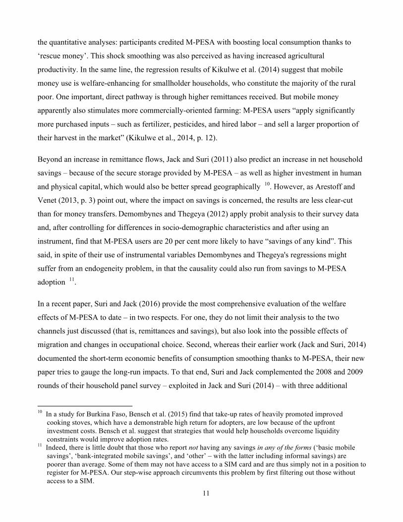
the quantitative analyses: participants credited M-PESA with boosting local consumption thanks to
‘rescue money’. This shock smoothing was also perceived as having increased agricultural
productivity. In the same line, the regression results of Kikulwe et al. (2014) suggest that mobile
money use is welfare-enhancing for smallholder households, who constitute the majority of the rural
poor. One important, direct pathway is through higher remittances received. But mobile money
apparently also stimulates more commercially-oriented farming: M-PESA users “apply significantly
more purchased inputs – such as fertilizer, pesticides, and hired labor – and sell a larger proportion of
their harvest in the market” (Kikulwe et al., 2014, p. 12).
Beyond an increase in remittance flows, Jack and Suri (2011) also predict an increase in net household
savings – because of the secure storage provided by M-PESA – as well as higher investment in human
and physical capital, which would also be better spread geographically 10. However, as Arestoff and
Venet (2013, p. 3) point out, where the impact on savings is concerned, the results are less clear-cut
than for money transfers. Demombynes and Thegeya (2012) apply probit analysis to their survey data
and, after controlling for differences in socio-demographic characteristics and after using an
instrument, find that M-PESA users are 20 per cent more likely to have “savings of any kind”. This
said, in spite of their use of instrumental variables Demombynes and Thegeya's regressions might
suffer from an endogeneity problem, in that the causality could also run from savings to M-PESA
adoption 11.
In a recent paper, Suri and Jack (2016) provide the most comprehensive evaluation of the welfare
effects of M-PESA to date – in two respects. For one, they do not limit their analysis to the two
channels just discussed (that is, remittances and savings), but also look into the possible effects of
migration and changes in occupational choice. Second, whereas their earlier work (Jack and Suri, 2014)
documented the short-term economic benefits of consumption smoothing thanks to M-PESA, their new
paper tries to gauge the long-run impacts. To that end, Suri and Jack complemented the 2008 and 2009
rounds of their household panel survey – exploited in Jack and Suri (2014) – with three additional
!!!!!!!!!!!!!!!!!!!!!!!!!!!!!!!!!!!!!!!!!!!!!!!!!!!!!!!!!!!!!10 In a study for Burkina Faso, Bensch et al. (2015) find that take-up rates of heavily promoted improved
cooking stoves, which have a demonstrable high return for adopters, are low because of the upfront investment costs. Bensch et al. suggest that strategies that would help households overcome liquidity constraints would improve adoption rates.
11 Indeed, there is little doubt that those who report not having any savings in any of the forms (‘basic mobile savings’, ‘bank-integrated mobile savings’, and ‘other’ – with the latter including informal savings) are poorer than average. Some of them may not have access to a SIM card and are thus simply not in a position to register for M-PESA. Our step-wise approach circumvents this problem by first filtering out those without access to a SIM.

! 12
rounds (conducted in 2010, 2011, and 2014). To identify the causal effects of M-PESA they use
changes in access to mobile money – quantified by the number of M-PESA agents within one kilometer
of the household – rather than adoption itself. Specifically, they compare outcomes, as measured in the
2014 survey, of households that saw large increases in agent density between 2008 and 2010 with
outcomes of households that experienced smaller increases over the same period.
Suri and Jack estimate that access to M-PESA effectively raised per capita consumption and lifted at
least 194,000 Kenyan households, or 2% of the total, out of poverty. They point out that the higher
observed consumption levels could be driven by multiple mechanisms, and find some support for the
savings and occupational choice channels. In particular, they find that an increase in M-PESA agent
density positively affects total financial savings of households – though not savings on M-PESA itself.
Also, individuals who experienced larger increases in M-PESA access were less likely to be working in
farming and more likely to be working in “business or sales”.
Suri and Jack also provide tentative evidence concerning the financial ‘stepping stone’ effect of
M-PESA anticipated by other authors. Mbiti and Weil (2014), for example, predict that generalised
adoption of M-PESA in Kenya would in the long run increase the proportion of banked people by 28
percentage points and in this way provide financial security to a greater share of the population. This
view is also embraced by Klapper and Singer (2014), who assume that M-PESA could be “an entry
point into the financial system” for the unbanked. Suri and Jack, in their regressions, find that the
change in access to mobile money effectively predicts the adoption of a bank account. They are,
however, quick to point out that this “may be driven by the supply-side response as banks began either
competing with mobile money or collaborating with M-PESA to create bank accounts like M-Shwari”
(Suri and Jack, 2016, p. 1291).
Finally, perhaps the most interesting result of Suri and Jack relates to the empowerment of women,
which is a key issue in Kenya. Indeed, several articles focus on rural areas or urban slums, where
gender inequalities are strong, especially when it comes to the household economy management.
Morawczynski and Pickens (2009) and Jack and Suri (2011) already saw great improvement in women
independence thanks to more regular and immediate remittances. The explanation would seems to be
that in patriarchal households the privacy offered by M-PESA as a store of value gives greater power to
women, who can manage the household liquidity with less control by the male head. Suri and Jack
(2016) further underpin this beneficial effect: their regressions show that consumption growth, the
reduction in poverty, and the switch away from subsistence agriculture into business or retail are all

! 13
more pronounced for female-headed households.
4. Data
The survey that we exploit was conducted between 2011 and 2013 as part of InterMedia’s Financial
Inclusion Insights Program, which is supported by the Bill & Melinda Gates Foundation. It covers eight
countries (Kenya, Nigeria, Tanzania, Uganda, Bangladesh, India, Indonesia, and Pakistan) and aimed
to gather information about financial behaviour at the household level. Households were chosen
randomly, based on the latest available census.
Table 2. Descriptive statistics (N = 3,000)
Percentage
M-PESA users 72.7 Bank account owners 28.2 Age
15-25 22.3 26-30 17.2 31-35 13.1 36-40 12.2 41-55 20.8 Over 55 14.4
Gender Female 62 Male 38
Education No education 33.3 Primary 39.1 Secondary 25.6 College 2.0
Urbanity (Urban = 1) 36.7
As explained, we focus on Kenya, for which the data pertain to 2013. Table 2 contains selected
descriptive statistics. Table A.1 in the Appendix contains the full set. The proportion of owners of an
M-PESA account (72.7 per cent) is consistent with the ratios found in the literature (see Section 2). The
proportion of bank account owners (28.2 per cent) is lower than the 55.2 per cent given by
Demirgüç-Kunt and Klapper (2014). This is due to our focus on bank accounts, while Demirgüç-Kunt
! 14
and Klapper also consider accounts at other financial institutions.
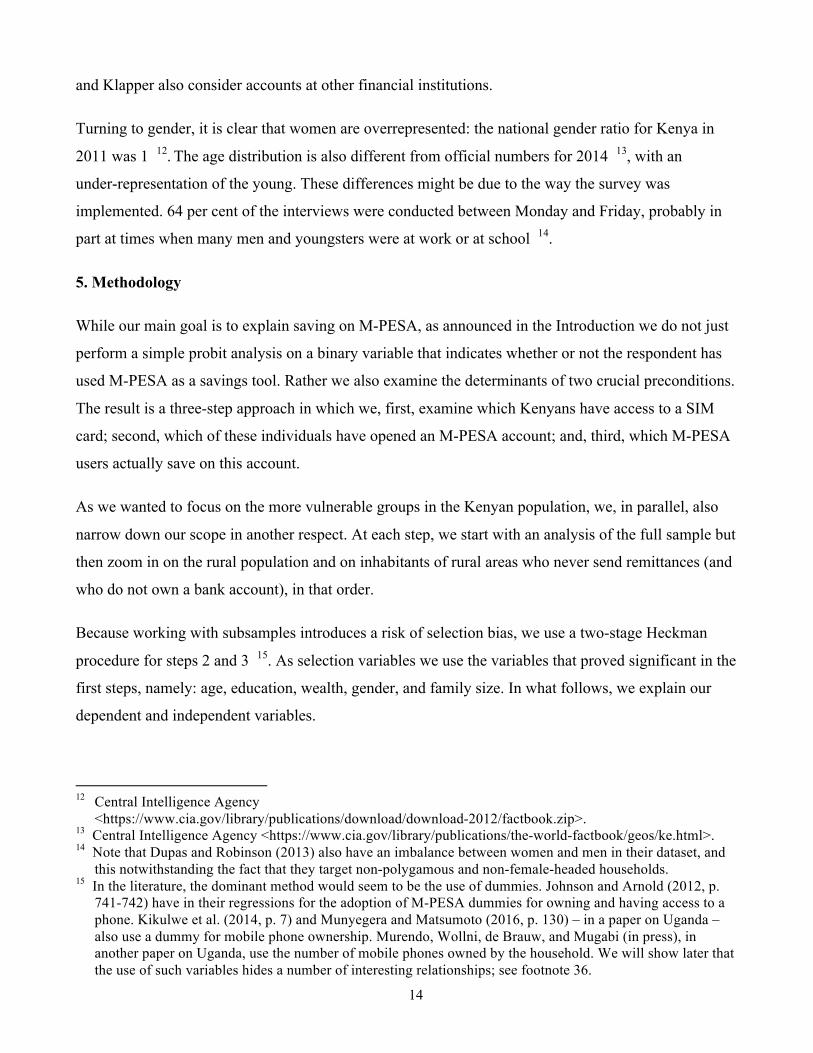
Turning to gender, it is clear that women are overrepresented: the national gender ratio for Kenya in
2011 was 1 12. The age distribution is also different from official numbers for 2014 13, with an
under-representation of the young. These differences might be due to the way the survey was
implemented. 64 per cent of the interviews were conducted between Monday and Friday, probably in
part at times when many men and youngsters were at work or at school 14.
5. Methodology
While our main goal is to explain saving on M-PESA, as announced in the Introduction we do not just
perform a simple probit analysis on a binary variable that indicates whether or not the respondent has
used M-PESA as a savings tool. Rather we also examine the determinants of two crucial preconditions.
The result is a three-step approach in which we, first, examine which Kenyans have access to a SIM
card; second, which of these individuals have opened an M-PESA account; and, third, which M-PESA
users actually save on this account.
As we wanted to focus on the more vulnerable groups in the Kenyan population, we, in parallel, also
narrow down our scope in another respect. At each step, we start with an analysis of the full sample but
then zoom in on the rural population and on inhabitants of rural areas who never send remittances (and
who do not own a bank account), in that order.
Because working with subsamples introduces a risk of selection bias, we use a two-stage Heckman
procedure for steps 2 and 3 15. As selection variables we use the variables that proved significant in the
first steps, namely: age, education, wealth, gender, and family size. In what follows, we explain our
dependent and independent variables.
!!!!!!!!!!!!!!!!!!!!!!!!!!!!!!!!!!!!!!!!!!!!!!!!!!!!!!!!!!!!!12 Central Intelligence Agency
<https://www.cia.gov/library/publications/download/download-2012/factbook.zip>. 13 Central Intelligence Agency <https://www.cia.gov/library/publications/the-world-factbook/geos/ke.html>. 14 Note that Dupas and Robinson (2013) also have an imbalance between women and men in their dataset, and
this notwithstanding the fact that they target non-polygamous and non-female-headed households. 15 In the literature, the dominant method would seem to be the use of dummies. Johnson and Arnold (2012, p.
741-742) have in their regressions for the adoption of M-PESA dummies for owning and having access to a phone. Kikulwe et al. (2014, p. 7) and Munyegera and Matsumoto (2016, p. 130) – in a paper on Uganda – also use a dummy for mobile phone ownership. Murendo, Wollni, de Brauw, and Mugabi (in press), in another paper on Uganda, use the number of mobile phones owned by the household. We will show later that the use of such variables hides a number of interesting relationships; see footnote 36.

! 15
5.1. Dependent Variables
As explained above, we use three different dependent variables: access to a SIM card, adoption of
M-PESA among potential users (that is, people having access to a SIM card), and, finally, use of
M-PESA as a savings tool. All three variables are on the individual level and are of a binary nature.
The first variable takes a value of 1 when the respondent either personally owns one or more SIM
cards, or can use somebody else’s. Apparently the latter is sufficient for having an M-PESA account: of
the 377 respondents who do not own a SIM card but have access to one, 38 reported owning an
M-PESA account.
Our second dependent variable, adoption of M-PESA, is self-explanatory. For the saving variables we
exploit questions where M-PESA users were asked whether or not they had already saved money for a
future purchase or payment on, respectively, M-PESA, M-SHWARI, M-KESHO, or on a bank account.
Surprisingly, literally none report that they save on an M-KESHO account, which leaves us with three
types of saving. As we are interested in the impact of M-PESA on financial inclusion, we decided to
merge, in a variable ‘saving on MFS’, the categories ‘saving on M-PESA’ (that is, on the “mobile
money account”) and ‘saving on M-SHWARI’, even though the first type of saving is non-interest
bearing while the second is.
Making a clear cut-off between the two types would have been difficult anyway. One reason is that the
survey asks respondents whether they have “ever” saved on a specific means 16. This implies that
M-PESA users who initially only saved on their mobile account, but later migrated to M-SHWARI
should normally have answered ‘yes' on both accounts (pun intended). The survey questions may also
have confused respondents. Indeed, a respondent who only ever has saved on M-SHWARI might also
incorrectly have answered ‘yes' on the question about saving on a mobile money account (because
M-SHWARI requires an M-PESA account). In our sample, of the 40 respondents who (have) save(d)
on M-SHWARI, 16 report that they (have) also save(d) on M-PESA. To be clear: the category ‘saving
on MFS’ (228 respondents, 7.6 per cent of the sample, 10.5 per cent of M-PESA users) is in practice
dominated by respondents who save on M-PESA but not on M-SHWARI; these respondents number
189, equivalent to 82.5 per cent of all MFS savers. Respondents who save only on M-SHWARI or on !!!!!!!!!!!!!!!!!!!!!!!!!!!!!!!!!!!!!!!!!!!!!!!!!!!!!!!!!!!!!16 For saving on M-PESA the question was: “Have you ever used a mobile money account to do the following?
[...] Save money for a future purchase or payment.” When cross-tabulating the answers to this question with ownership of an M-PESA account, we discovered that there were 5 respondents who answered ‘yes', whereas they do not personally own a mobile money account (M-PESA or other). All 5 do declare having already made use of M-PESA. A possible scenario is that these individuals stopped using M-PESA because they now save on somebody else’s account.

! 16
both M-SHWARI and M-PESA make up respectively 10.4 per cent and 7.0 per cent of MFS savers.
As already announced at the end of Section 3.2, because of the more stringent definition (saving for a
future purchase or payment) the incidence of saving in our dataset – 10.5 per cent of the M-PESA users
– is markedly lower compared to the headline figures reported in earlier studies 17. But on closer
scrutiny it can be reconciled with the more detailed results reported by Johnson et al. (2012) and
Johnson (2014, 2016). In Johnson’s 2010/2011 survey, the main reasons given for holding a balance on
one’s phone were (multiple responses allowed): “because it is safer” (19 per cent of registered
M-PESA users), “in order to have funds to send to family/relatives/friends when they need them” (18
per cent), “to buy airtime” (9 per cent), “in order to run my business easily” (7 per cent), “efficient,
gives financial flexibility, available when needed” (5 per cent), “emergencies/unexpected needs” (4 per
cent), “because it is the only place I have to save money safely” (4 per cent), “so that I can keep funds
there and then transfer them to another saving place” (3 per cent), …, “so that I can save there and then
transfer to a bank account” (2 per cent), etc. (Johnson et al., 2012a, p. 25, Table 4) 18. As can be seen,
the reasons that would qualify as ‘saving’ under our definition all run in the low single digits.
A final note is that the category ‘saving on a bank account’ (139, or 4.6 per cent of the sample), which
we will examine as a point of comparison, is potentially quite diverse and might comprise respondents
who do not have a mobile money account, respondents who already had a bank account before they
started using M-PESA (maybe, in part, to have a remote control), and – given the not so accurate
phrasing of the survey questions – possibly also M-SHWARI users who do not have a bank account
apart from the CBA account that comes with M-SHWARI (see Section 2). Of the 40 people who (have)
save(d) on M-SHWARI, 7 report that they (have) also save(d) on a bank account.
We now discuss our independent variables.
5.2. Independent Variables
Demographic variables allow us to understand the social conditions of the respondents. We choose the
ones that are commonly used in the studies adopting the socio-individual approach (see Section 3.1),
namely: age, gender, wealth, education level, literacy, geographical situation (urban or rural), and
!!!!!!!!!!!!!!!!!!!!!!!!!!!!!!!!!!!!!!!!!!!!!!!!!!!!!!!!!!!!!17 Studies for other countries also report substantially higher numbers. Murendo and Wollni (2016), for
example, interviewed 482 households in 39 rural villages in Uganda. In their research, 57 per cent of the mobile money users stated that they use their mobile money account as a savings account.
18 Johnson (2014, p. 12) and Johnson (2016, p. 92) report higher percentages, but these are in fact absolute numbers; see the second column of Table 4 in Johnson (2012a, p. 25).

! 17
family size. Table A.1 provides descriptive statistics.
Our choice of age phases was driven by the possible association between age and the motivations to
save. In rural Kenya, where the population mainly consists of farmers, the propensity to save follows a
hump-shaped curve (Kibet, Mutai, Ouma, Ouma, & Owuor, 2009). Many 15-25-year-olds still depend
on their parents or are not able to put money aside. People in the 25-40 age bracket are typically
responsible for their household and tend to save in order to improve their financial security. The
effective retirement age in Kenya used to be 55. In 2009 it was put at 60 for certain professions (Were,
2009). We nevertheless keep 55 as the switch point, for we assume that the law did not yet have a
significant impact in 2013 (when our data was collected). In short, the age range 40-55 is probably
associated with intense savings to prepare retirement, followed by a decrease after 55, due to the fall in
income.
Turning to wealth, in the Financial Inclusion Insights Program survey respondents are only asked about
three categories of tools they own 19. We used this information to build an index, ranging between 0
and 7, based on the number of tools declared. Our ‘wealth’ variable is thus of a completely different
nature compared to studies for the developed world. It is more of an inverted poverty index 20.
For education we look at the highest level of schooling completed by the respondent. In the survey,
respondents were also asked to accomplish a basic reading task. This allowed us to create a dummy that
considers someone as literate as soon as he or she was not placed in the lowest category (“unable to
read/understand the informed consent form”) for either reading or understanding. A numeracy variable
proved redundant, for the t-tests showed a high correlation with literacy.
6. Results
As announced, we first examine Kenyans’ possession of or access to a SIM card, as this is
indispensable to own an M-PESA account. In sections 6.2 and we then focus on, respectively, the
adoption of M-PESA in general (that is, for any type of use) and the use of M-PESA as a savings tool.
!!!!!!!!!!!!!!!!!!!!!!!!!!!!!!!!!!!!!!!!!!!!!!!!!!!!!!!!!!!!!19 Tools asked about: iron (charcoal or electric), number of mosquito nets (three possible answers: “0”, “1”, “2
or more”), number of towels (three possible answers: “0”, “1”, “2 or more”), number of frying pans (three possible answers: “0”, “1”, “2 or more”),
20 Other authors have used similar approaches. The income estimates of Johnson, Brown and Fouillet (2012b, p. 25), for example, are based on household characteristics and assets (fridge, radio/cd, iron, etc.). See also Johnson and Arnold (2012).

! 18
6.1. Precondition: SIM card access
Table 3 presents the results of our regressions for, respectively, ownership of and access to a SIM card.
To be clear, the second variable encompasses the first: 82 per cent of our sample own a SIM card, but
in addition quite a few respondents can use the SIM card of a relative or a friend, so that overall 94.6
per cent ‘have access to’ a SIM card. In other words, (only) 5.4 per cent of our sample are simply not in
a position to open an M-PESA account 21.
Table 3. Possession of and access to a SIM card
Urban + Rural Rural Rural non-senders Possession
(1) Access
(2) Possession
(3) Access
(4) Possession
(5) Access
(6) Outcome eq.
Age ** n.s. * n.s. n.s. n.s. 15-25 – – – – – – 26-30 0.479*** 0.369* 0.435*** 0.401* 0.403** 0.397 (4.85) (2.25) (3.47) (2.01) (2.70) (1.84) 31-35 0.481*** 0.262 0.515*** 0.326 0.479** 0.382 (4.55) (1.61) (3.92) (1.67) (3.12) (1.77) 36-40 0.583*** 0.287 0.581*** 0.222 0.446** 0.111 (5.24) (1.71) (4.39) (1.17) (2.78) (0.53) 41-55 0.517*** 0.294* 0.534*** 0.352* 0.472*** 0.297 (5.68) (2.16) (4.89) (2.24) (3.58) (1.73) Over 55 0.192* -0.0204 0.227* 0.0839 0.160 0.0956
(2.00) (-0.15) (2.01) (0.55) (1.17) (0.56) Gender (Female = 1) -0.178** -0.152 -0.124 -0.118 -0.113 -0.0916 (-2.80) (-1.63) (-1.67) (-1.12) (-1.25) (-0.78) Education *** *** *** *** *** ***
Non-educated – – – – – – Primary 0.545*** 0.678*** 0.530*** 0.680*** 0.443*** 0.615*** (7.88) (6.17) (6.47) (5.16) (4.33) (4.00) Secondary 0.974*** 0.874*** 0.950*** 1.016*** 0.761*** 0.671* (9.80) (5.13) (7.29) (3.92) (4.04) (2.15) College No
variation No
variation No
variation No
variation No
variation No
variation Literacy 0.00769 -0.128 0.0143 -0.0748 -0.000429 -0.143 (0.11) (-1.17) (0.17) (-0.60) (-0.00) (-1.02) Wealth 0.186*** 0.250*** 0.210*** 0.285*** 0.184*** 0.299*** (11.17) (9.40) (10.38) (8.95) (7.26) (8.10) Family size -0.037*** 0.00928 -0.0132 0.0323 -0.00459 0.0389* (-3.62) (0.62) (-1.14) (1.83) (-0.34) (2.01) Constant -0.149 0.548** -0.438** 0.206 -0.590*** 0.0457 (-1.26) (3.14) (-2.99) (1.00) (-3.33) (0.20) Pseudo R2 0.18 0.23 0.18 0.24 0.11 0.19 AIC 2322 994 1678 779 1204 665 BIC 2394 1065 1745 845 1262 724 Log likelihood -1149 -485 -827 -378 -590 -321 Observations 2934 2934 1874 1874 994 994 t statistics in parentheses; *, ** and *** indicate significance at the 0.05, 0.01 and 0.001 level, respectively
!!!!!!!!!!!!!!!!!!!!!!!!!!!!!!!!!!!!!!!!!!!!!!!!!!!!!!!!!!!!!21 In principle, one needs to be 18 or older to open an M-PESA account, but in practice there are younger
respondents who have one – perhaps because their parents have opened an account for them.

! 19
Before we discuss the results, let us point out that while one would expect the education variable and
the literacy dummy to be natural alternatives (which should not appear in one and same regression),
oddly enough they proved to be correlated negatively (N = 2,996: t = 2.0; p = 0.04). We therefore
included both in our regressions. We can already reveal that the literacy variable will at best be
marginally significant.
If we then focus first on the full sample, we can see in regression (1) that, overall, those who are older
than 25, male, educated, and are part of a ‘wealthy’ (in fact: non-poor) household have a higher
probability of owning a SIM 22. Conversely, the higher the family size, the lower the probability. An
examination of the average marginal effects (AMEs) reveals, first of all, that the higher the education
level, the stronger the effect: completion of primary education increases the probability of owning a
SIM card by 12 percentage points compared to the non-educated, completion of secondary education
increases it by 21 percentage points, and literally all respondents who have completed university own a
SIM card; hence the “no variation” in Table 3. Turning to age, here too the effect increases in size as
we move up the categories, but only up to a point (namely the 36-40 age bracket). Note in particular
that while those over 55 do have a higher probability to own a SIM card than the 15-25 age group, at 4
percentage points the AME is substantially smaller than for all other age ranges (for which the AMEs
lie in the 10 to 13 percentage points range). This might be an indication of technology aversion. But
especially the difference between regressions (1) and (2) catches the eye. Once we broaden the
dependent variable to those who do not own but have access to a SIM card, all of a sudden gender and
family size play no role anymore, age becomes less significant, and the AMEs of education and wealth
become substantially smaller (as do those of age). The general picture that emerges is one where some
of the young, the women, and those in bigger households can use the SIM of a family member or
friend. This system of shared ownership increases the reach of telecom services (and thus, at least in
principle, of MFS), but as the results for education and wealth (and, when added, also urbanity)
indicate, there is a group that is excluded from even this indirect access. Worryingly, in line with the
results of Murphy and Priebe (2011, p. 5), this group is disproportionately composed of non-educated
individuals who are part of a poor household living in rural areas 23.
!!!!!!!!!!!!!!!!!!!!!!!!!!!!!!!!!!!!!!!!!!!!!!!!!!!!!!!!!!!!!22 When added, urbanity also has a very significant positive effect. 23 From a methodological angle, let us point out that, in their paper on Uganda, Murendo et al. (in press) also
find that poor households have a lower probability to own a mobile phone, but only indirectly. Murendo et al. find that the number of mobile phones owned by the household has a significant positive impact on the adoption of mobile money, and when they split their sample into poor and non-poor households it becomes clear that the impact is substantially bigger for poor households (Murendo et al., in press, p. 12, Table 5). Our three-step approach has the advantage of directly uncovering such relationships.

! 20
This pattern is also evident in regressions (3)-(4) and (5)-(6), where we progressively zoom in on the
more vulnerable groups in the Kenyan population. The rural population is vulnerable to weather
hazards, which translates into volatile food prices and uncertain incomes. Such individuals are on
average probably less able to cope with shocks. Among the rural population, many of those who never
send any remittances are probably in a situation of strong financial dependence, and thus even more
vulnerable to financial hazards. However, we noticed that some of these ‘non-senders’ do own a bank
account, which is a sign of relative wealth. We therefore excluded these individuals and in (5)-(6) only
consider the unbanked among the rural non-senders.
As can be seen, the results of regressions (3)-(6) are similar to those for the full sample, even though
the negative impact of family size on SIM ownership loses its significance, gender is now at best
significant at the 10 per cent level, and the presumed technology aversion of the +55 becomes slightly
more salient. But, importantly, the beneficial effect of shared ownership of SIMs is even more
prominent than for the full sample, and increasingly so the more we zoom in on the more vulnerable
groups. While only 77.4 per cent of the rural population own a SIM, 92.7 per cent have access to one,
which implies an increase in reach of 15.3 percentage points (compared to +12.6 for the full sample).
For the rural non-senders, these numbers are 61.6 per cent, 86.5 per cent, and 24.9 percentage points.
Just as for the full sample, those who do not have access to a SIM are predominantly non-educated and
poor. Stronger still, the AMEs of education and wealth increase in size when we move from the full
sample to the rural sample, and a second time when we move from the latter to the rural non-senders.
Interestingly, family size – which for the full sample has a significant negative impact on SIM
ownership – now has a significant positive impact on access in regression (6).
6.2. M-PESA adoption
In Table 4 we explain the possession of M-PESA by those respondents who are in a position to adopt;
that is, who at least have access to a SIM card 24. As a point of comparison we also explain the
possession of a bank account. From regression (4) onward we again zoom in on the more vulnerable
population groups.
!
!!!!!!!!!!!!!!!!!!!!!!!!!!!!!!!!!!!!!!!!!!!!!!!!!!!!!!!!!!!!!24 One could argue that we should have restricted our sample even more, namely to respondents who have
access to a SIM of Safaricom, the mobile provider behind M-PESA. However, while we can identify which SIM(s) people own, the survey question about access to a SIM does not inquire about the provider. Reassuringly, of the respondents who own a SIM, 94 per cent have a Safaricom SIM (either exclusively or as one of their SIMs, respectively 70 per cent and 24 per cent).

! 21
Table 4. Possession of formal accounts by individuals who have access to a SIM card
Urban + Rural
Rural
Rural non-senders
M-PESA M-PESA Bank account M-PESA M-PESA (1) (2) (3) (4) (5)
Outcome equation Age *** *** *** * **
15-25 – – – – – 26-30 0.380*** 0.345*** 0.462*** 0.347** 0.123 (4.46) (4.17) (5.04) (2.77) (1.09) 31-35 0.492*** 0.391*** 0.502*** 0.512*** 0.358* (5.21) (4.31) (5.09) (3.40) (2.16) 36-40 0.608*** 0.485*** 0.678*** 0.578*** 0.451* (6.14) (5.09) (6.79) (3.41) (2.40) 41-55 0.573*** 0.432*** 0.829*** 0.654*** 0.567** (6.83) (5.43) (9.34) (3.68) (2.73) Over 55 0.508*** 0.254** 0.829*** 0.569** 0.553**
(5.36) (2.90) (8.12) (2.89) (2.74) Gender (Female = 1) -0.105 -0.182** -0.520*** -0.102 -0.0541 (-1.81) (-3.25) (-9.25) (-1.23) (-0.71) Education *** *** *** ***
Non-educated – – – – – Primary 0.401*** 0.334*** 0.489*** 0.595*** (6.00) (4.27) (6.04) (7.57) Secondary 0.811*** 1.029*** 0.929*** 1.248*** (9.27) (11.77) (7.50) (8.87) College 1.161*** 2.188*** 6.848 No variation
(3.58) (8.82) (0.00) Literacy 0.118 0.109 -0.0354 0.0972 0.141 (1.92) (1.81) (-0.55) (1.22) (1.61) Wealth 0.0932*** 0.146*** 0.153*** 0.152*** 0.126*** (5.79) (10.55) (8.74) (7.39) (5.78) Family size -0.0505*** -0.0691*** -0.0388*** -0.0386 -0.0535** (-4.78) (-6.80) (-3.42) (-1.53) (-3.29) Constant -0.0763 0.317** -1.717*** -0.431 0.0135 (-0.66) (3.23) (-12.00) (-0.95) (0.03)
Selection equation Age -0.0193 -0.00922 -0.00883 0.110*** -0.0202 (-0.79) (-0.38) (-0.36) (7.92) (-1.36) Education 0.550*** 0.643*** 0.542*** -0.185*** -0.480*** (7.14) (8.43) (6.97) (-5.47) (-12.41) Wealth 0.253*** 0.242*** 0.252*** -0.00208 -0.0906*** (9.78) (9.45) (9.57) (-0.16) (-6.37) Gender -0.113 -0.0847 -0.153 -0.174*** 0.0774 (-1.22) (-0.92) (-1.64) (-3.43) (1.42) Family size 0.0143 0.0202 0.0151 0.108*** 0.0669*** (0.97) (1.36) (0.99) (10.61) (6.72) athrho -0.962* -1.299* 0.379 -0.181 -1.172 (-2.18) (-2.49) (0.60) (-0.38) (-1.28) Chi2 6.3 27.5 0.63 0.15 1.1 p 0.012 0.000 0.429 0.695 0.292 Log likelihood -1831 -1880 -1874 -2767 -2128 Censored 162 162 162 1238 2135 Uncensored 2832 2832 2832 1756 859 t statistics in parentheses; *, ** and *** indicate significance at the 0.05, 0.01 and 0.001 level, respectively

! 22
If we then discuss our results in the order in which the variables appear in Table 4, we first observe
that, with the exception of the 26-30-year-olds in regression (5), every age range has a significantly
higher probability to own an M-PESA account than the 15-25. This is fairly unusual, in that the young
are typically among the early adopters of new technologies 25. However, the innovation we examine in
this paper has a crucial financial dimension. As we pointed out in Section 5.1, a substantial portion of
the 15-25-year-olds may still depend on their parents. Even in developed countries, it is therefore not
exceptional to see that the youngest do not use the latest in payment technologies. For example, where
the Netherlands are concerned, Jonker (2007) finds that younger consumers between the age of 15 and
24 are the heaviest cash users, even more so than those over 65.
Turning to gender, it is of crucial importance to factor in the multicollinearity between gender and
education, in that women are, on average, less educated than men (N = 2996: t = 5.1; p = 0.00). Indeed,
regression (2) – where we have omitted the education variable – gives the impression that there is a
gender effect. However, once education is included in regression (1) – and also in regressions (4) and
(5) for the rural subsamples – we find that gender as such does not restrict women’s access to M-PESA.
Note that Johnson and Arnold (2012, p. 742) also find an insignificant effect of gender on M-PESA
adoption. There is, however, a gender effect for the possession of a bank account, in regression (3).
This is plausible in a patriarchal society such as Kenya, where in most households the male head will
be the owner of the account 26, not unlike for the mobile phone. For education itself, we find, as
expected and in line with Johnson and Arnold (2012), that the educated have a higher probability of
owning an M-PESA account 27. Note also that the AMEs (not reported) increase with the education
level. Both observations also hold – in fact even more strongly so – for the possession of a bank
account in model (3). To be clear: in model (5), all respondents who have completed college own an
M-PESA account.
The impact of literacy is less apparent than expected: it is only significant at the 10 per cent level in
regressions (1) and (2). It is also relatively small: being literate increases the probability of owning an
M-PESA account with 3 percentage points. Note that Porteous (2007) explains that literacy is in fact
!!!!!!!!!!!!!!!!!!!!!!!!!!!!!!!!!!!!!!!!!!!!!!!!!!!!!!!!!!!!!25 At first sight, this result would also seem to clash with those of Johnson and Arnold (2012, p. 741) and
Kikulwe et al. (2014), neither of which find a significant effect of age. But then in both papers age is entered as a continuous variable. In addition, Kikulwe et al. (2014) work with household-level data and use age of the household head.
26 Dupas and Robinson (2013) reveal that in rural areas 10 per cent of the women have a bank account while for men this number is 21 per cent.
27 Kikulwe et al. (2014, p. 7, Table 3) find a significant positive effect of the education level of the household head.

! 23
not enough to describe people's ability to use a formal account, and speaks of “financial capability” 28,
which makes our result even more surprising. Still, apparently the bulk of the Kenyan population is
able to use M-PESA. Maybe this is because the required skills are basic, maybe people get help from
family members or M-PESA agents.
‘Wealth’ is positively correlated to adoption across the board. Being below a minimum threshold of
possession of essential tools apparently precludes M-PESA adoption, which seems logical. Finally,
family size has a negative effect on the adoption of M-PESA. It is not significant for the rural
subsample in (4), but becomes significant again once the remittance senders and bank account owners
have been filtered out.
To complete the profile of M-PESA users, it can be noted that, when introduced in models (1) and (2),
urbanity is positive and highly significant (not reported). The same is true if possession of a bank
account is added to models (1), (2) and (4). This is not surprising given that regression (3) shows that
the possession of a bank account is explained by the same variables as the possession of an M-PESA
account 29. We find that 91 per cent of the banked population also use M-PESA, compared to 65 per
cent of the unbanked. This is a strong indication that M-PESA and banks are complementary, at least
for the bank account owners 30. However, the relative importance of the unbanked among the M-PESA
users has clearly increased over the years. Jack and Suri (2014) found that the unbanked accounted for
25 per cent of M-PESA users in 2008, and 50 per cent in 2009. We find that in 2013, at least 64 per
cent of M-PESA users were previously unbanked.
To conclude, even though higher education, bank account possession, urbanity, and higher ‘wealth’
still significantly increase the probability of owning an M-PESA account – four results that are in line
with Aker and Mbiti – we notice a general tendency of democratisation of M-PESA.
6.3. Saving
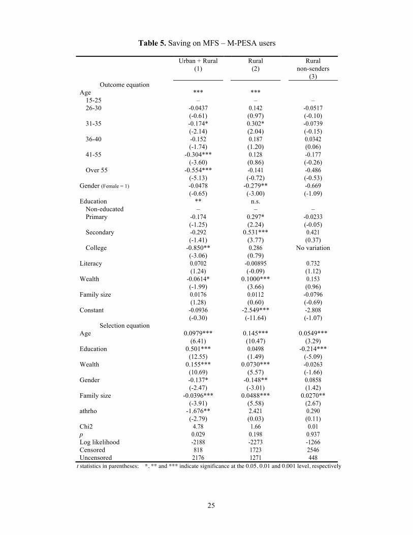
In Table 5 we now analyse which factors increase M-PESA users’ propensity to save 31. As mentioned
!!!!!!!!!!!!!!!!!!!!!!!!!!!!!!!!!!!!!!!!!!!!!!!!!!!!!!!!!!!!!28 The understanding of financial topics and the ability to put that knowledge into practice. 29 Note that our results in regression (3) are consistent with those of Allen et al. (2012), who find, for formal
accounts in general, that adopters are mainly male, urban, and relatively well-off. 30 Arestoff and Venet (2013, p. 4) call this the “additive model” of mobile banking: “People already have a bank
account and new financial services become available through their mobile phone”. We are more interested in the “converted model”, where people (especially the poor) replace informal by formal services.
31 As a reminder: ‘saving on MFS' comprises both respondents who save only on an M-SHWARI account and those who save on M-PESA; see Section 5.1. In regressions 2 and 3 we encountered non-concavity issues so

! 24
in the literature review, saving can be understood in many ways. We use the definition of the survey
(see Section 5), which also happens to correspond best to the behaviour we want to observe.
In Table 5 two observations stand out. The first is that in regression (1) several variables now have a
negative sign. For age this is not surprising across the board. As explained in Section 5.2, after
retirement a decrease in the propensity to save is only normal. However, we also find a very significant
negative coefficient for the 41-55 age category and a less significant one for the 31-35 category. We
have no ready explanation for these results. To continue, the negative coefficients for education and
wealth are indications that the richer respondents are less likely to save on MFS because they have
other alternatives, such as bank accounts 32.
The second major observation is that several of the socio-demographic characteristics that proved
important in the previous two steps now play almost no role anymore, especially not in regression (3)
for the most vulnerable group. In fact, in regression (3) simply none of the variables in the outcome
equation is significant. In other words, we are unable to explain the saving behaviour in this subgroup.
This is probably due to the low variation in the dependent variable: out of the 448 individuals in this
regression, a mere 12 (or 2.2 per cent) save on MFS. We therefore concentrate on regression (2).
In regression (2), the impact of education and wealth does not surprise. Gender has its usual negative
sign and is significant at the 1 per cent level 33. An analysis of the average marginal effects indicates
that among the rural population women are 2.1 percentage points less likely to save than men. At first
sight, the gender effect would thus seem limited. However, given that, overall, only 5.4 per cent of the
rural population saves on MFS, the impact of gender, controlling for education, is in fact very
substantial. Note also that the impact increases the more one focuses on the vulnerable groups –
although cautiousness is warranted, because gender is not significant in regressions (1) and (3). In the
full sample (where 7.6 per cent saves on MFS), the AME of gender is 1.6 percentage points; among the
rural non-senders the corresponding figures are 1.2 per cent and 2.8 percentage points.
!!!!!!!!!!!!!!!!!!!!!!!!!!!!!!!!!!!!!!!!!!!!!!!!!!!!!!!!!!!!!!!!!!!!!!!!!!!!!!!!!!!!!!!!!!!!!!!!!!!!!!!!!!!!!!!!!!!!!!!!!!!!!!!!!!!!!!!!!!!!!!!!!!!!!!!!!!!!!!!!!!!!!!!!!!!!!!!!!!!!!!!!!!!!!!!!!!!!!!!!!!!!!!!!!instead of the default Stata method we had to use the “difficult” regression option for regression (2), and a combined Stata modified Berndt-Hall-Hall-Hausman, Newton-Raphson, Davidon-Fletcher-Powell, and Broyden-Fletcher-Goldfarb-Shanno (technique (bhhh 3 nr 3 dfp 3 bfgs 3)) optimisation method of the default Stata method for regression (3).
32 Note in this respect that the significance of wealth disappears when we add a dummy to the regression that captures whether or not the respondent sends remittances by way of M-PESA. The same is true when we limit the sample to the unbanked (N = 1,403). The picture that emerges is one of people living in the city who use M-PESA to send money to urban relatives but do not use it to save.
33 Note that Demombynes and Thegeya (2012) find that men are more likely to have savings of any kind (not just on their mobile account).
! 25
Table 5. Saving on MFS – M-PESA users
Urban + Rural (1)
Rural (2)
Rural non-senders
(3) Outcome equation
Age *** *** 15-25 – – – 26-30 -0.0437 0.142 -0.0517 (-0.61) (0.97) (-0.10) 31-35 -0.174* 0.302* -0.0739 (-2.14) (2.04) (-0.15) 36-40 -0.152 0.187 0.0342 (-1.74) (1.20) (0.06) 41-55 -0.304*** 0.128 -0.177 (-3.60) (0.86) (-0.26) Over 55 -0.554*** -0.141 -0.486
(-5.13) (-0.72) (-0.53) Gender (Female = 1) -0.0478 -0.279** -0.669 (-0.65) (-3.00) (-1.09) Education ** n.s.
Non-educated – – – Primary -0.174 0.297* -0.0233 (-1.25) (2.24) (-0.05) Secondary -0.292 0.531*** 0.421 (-1.41) (3.77) (0.37) College -0.850** 0.286 No variation
(-3.06) (0.79) Literacy 0.0702 -0.00895 0.732 (1.24) (-0.09) (1.12) Wealth -0.0614* 0.1000*** 0.153 (-1.99) (3.66) (0.96) Family size 0.0176 0.0112 -0.0796 (1.28) (0.60) (-0.69) Constant -0.0936 -2.549*** -2.808 (-0.30) (-11.64) (-1.07)
Selection equation Age 0.0979*** 0.145*** 0.0549*** (6.41) (10.47) (3.29) Education 0.501*** 0.0498 -0.214*** (12.55) (1.49) (-5.09) Wealth 0.155*** 0.0730*** -0.0263 (10.69) (5.57) (-1.66) Gender -0.137* -0.148** 0.0858 (-2.47) (-3.01) (1.42) Family size -0.0396*** 0.0488*** 0.0270** (-3.91) (5.58) (2.67) athrho -1.676** 2.421 0.290 (-2.79) (0.03) (0.11) Chi2 4.78 1.66 0.01 p 0.029 0.198 0.937 Log likelihood -2188 -2273 -1266 Censored 818 1723 2546 Uncensored 2176 1271 448
t statistics in parentheses; *, ** and *** indicate significance at the 0.05, 0.01 and 0.001 level, respectively

! 26
7. Discussion and conclusions
This paper has looked into the uptake and use of M-PESA mobile financial services in Kenya. In
particular, we wanted to find out to what extent the success of M-PESA as a money transfer mechanism
has also resulted in higher financial inclusion, which we equate with being able to save. To answer this
question, we exploit survey data collected among 3,000 respondents by InterMedia as part of the 2013
Financial Inclusion Insights Program. Specifically, we use a three-step probit procedure to identify the
socio-demographic characteristics of, successively, the respondents who do not have access to a SIM
card, have access to a SIM card but have not opened an M-PESA account, and, finally, have an
M-PESA account but do not save on it. Figures 1-3 summarise our main results.
The Figures should be read as follows. The first bar represents the total number of respondents in the
(sub)sample studied. The bars to the right then indicate, for each of the steps, how many overcome the
adoption barrier and how many are ‘left behind’. For example, in Figure 2 for the rural population the
second bar indicates that 92.7 per cent of the 1,899 individuals in the subsample, or 1,760, have access
to a SIM card 34, whereas 7.3 per cent have not (and are thus already financially excluded at this early
stage). In the next step, we then analyse which of the remaining 1,760 have an M-PESA account, and
so forth. As can be seen, eventually we are left with 103 respondents (or 5.4 per cent of the total) who
actually save on MFS. At each stage, the small arrows beneath the bars indicate which
socio-demographic characteristics explain the split-up in the next step. In other words, the arrows
summarise the results of, respectively, Tables 3, 4, and 5. The rationale behind the bigger arrows is
similar, yet different. These arrows summarise the results that are presented in Table A.2 in the
Appendix. In this table, we throw overboard our three-step approach and rather explain directly, for the
full (sub)samples (that is, irrespective of whether the respondents have access to a SIM or own an
M-PESA account), who saves on MFS or not. The goal here is primarily to highlight the value-added
of our three-step approach. Indeed, as we illustrate below, because an explanatory variable can be
crucial in one step but not in the next or, stronger, because the direction of its impact can differ
between steps, there may be little or no trace of its influence in a direct estimation as in Table A.2.
Another advantage of our three-step approach is that it provides a better insight into the nature of the
barriers to adoption.
!
!!!!!!!!!!!!!!!!!!!!!!!!!!!!!!!!!!!!!!!!!!!!!!!!!!!!!!!!!!!!!34 So, to be clear, for the first step in Figures 1-3 we use the results for access to a SIM, not those for possession.
We come back to this below.

! 27
!

! 28
To start with Figure 1 for the full sample, it can be seen that education and ‘wealth’ have a significant
positive impact in the first two steps but a (smaller) negative impact in step three. The latter is not
visible in the direct analysis because, overall, the positive impact dominates. This is a first instance
where our three-step approach provides added value. Another illustration is that age is significant in
steps two and three, but with a different sign so that its effect is absent in the direct analysis. Finally,
gender is a special case: it has a significant negative impact in the direct analysis, but it is not
significant in any of the three steps – at least not if one works with a 5 per cent significance cut-off. At
10 per cent, gender is significant in steps one and two; see regression (2) in Table 3 and regression (1)
in Table 4. We come back to this below.
The results for the rural population, in Figure 2, are very similar as far as education, wealth, and age are
concerned. The only difference is that education and wealth do not have a negative impact in step three.
Perhaps the most interesting result in Figure 2 is the gender effect in the final step (and in the direct
analysis): even after controlling for differences in education, female M-PESA users are less likely to
save.
Finally, our three-step analysis for the rural non-senders (in Figure 3) is handicapped by the fact that
we cannot explain the saving behaviour in the final step, probably due to the low variation (see section
6.3). But the results in steps one and two are very similar to those in Figures 1 and 2. Hence, a first
general conclusion is that those who do not benefit from the positive effects of M-PESA (such as the
ability to receive more frequent and faster remittances and, ultimately, the ability to save on a formal
account) are for the most part the non-educated and the poor.
Then there is the issue of financial empowerment of women thanks to M-PESA. Gender has a
significant negative effect in the direct analysis for all three samples – at the 1 per cent level in Figures
1 and 2, and at the 5 per cent level in Figure 3 – but our three-step analysis sends confusing signals. As
can be seen, gender is not significant in any of the steps in Figure 3, only in the final step in Figure 2,
and only at 10 per cent in steps one and two in Figure 1. It is, however, important to point out that in all
three Figures the selection criterion in step 1 is access to a SIM (not possession), so an implicit
assumption behind our three-step analysis is that it is sufficient to have access to a SIM (in step 1) to
ultimately be able to save (in step 3).
This raises the question whether this assumption is realistic. A closer analysis of the data by means of
t-tests showed, unsurprisingly, that respondents who have access to a SIM but do not own one have a

! 29
significantly lower probability to have an M-PESA account compared to respondents who have their
own personal SIM – and this for all three samples. However, it is not as if there are none. In the full
sample, for example, there are 43 respondents who do have an M-PESA account despite not owning a
SIM. So we could hardly throw away these observations. This said, there are barely any respondents
who save on MFS without owning a SIM: 3 in the full sample, 2 among the rural population, and one
single individual in our most narrow sample.
Taken together, these observations suggest that having access to a SIM without owning one might be
sufficient to open an M-PESA account (and thus to receive remittances 35), but that it is an entirely
different matter to entrust somebody else('s SIM) with your savings. In terms of methodology, this
suggests that when studying the gender effect one should perhaps select on SIM ownership in step 1
rather than on mere access. We may thus have been too positive about the beneficial effect of shared
ownership of SIMs in our analysis of Table 3.
When revisiting Table 3 with this new frame of mind, the gender effect indeed becomes more visible –
in line with the direct analysis. In regression (1) of Table 3, for the full sample, gender is significant at
the 1 per cent level and in regression (3), for the rural population, it is significant at 10 per cent. Also, if
we change the selection criterion in Table 4 to possession of a SIM instead of possession or access
(results not reported), the impact of gender drops dramatically. In regression (1) the AME goes from
-0.028 and a significance level of 10 per cent to an insignificant -0.008; in regression (4) the AME
drops from -0.026 to -0.012. In order words, this shows that women who own a SIM do not have a
lower probability to have an M-PESA account 36. The exclusion happens at an earlier stage (and is not
captured by our original three-step analysis because of the assumption that just having access to a SIM
is sufficient). !!!!!!!!!!!!!!!!!!!!!!!!!!!!!!!!!!!!!!!!!!!!!!!!!!!!!!!!!!!!!35 Among the respondents who have access to a SIM but do not own one (379 in the full sample), the receivers
of remittances (61) outnumber the senders (37). 36 The analysis in the main text may help understand why Johnson et al. (2012) and Johnson and Arnold (2012)
find different results for gender. Johnson et al. (2012, p. 21) find that “being a man significantly increases the likelihood of access compared to being a woman – a result we did not find in the analysis of the FinAccess 2009 data where gender was insignificant”. While the two papers use different samples collected in different years, the explanation might lie in the fact that, unlike Johnson et al. (2012), Johnson and Arnold (2012, p. 741-742) have in their regressions dummies for, respectively, owning and having access to a phone. These dummies, which have the biggest marginal effects on adoption of all the variables, probably capture the lower probability of women to own or have access to a phone and cause gender itself to be insignificant. Explained differently, Johnson et al. (2012), who do not control for phone ownership or access, in fact lump together steps 1 and 2 of our analysis, and the gender effect that they find probably relates mostly to exclusion in step 1 rather than step 2. Conversely, Johnson and Arnold (2012) do control for phone ownership/access and therefore have a cleaner analysis of step 2. In our view, this is another illustration of the value added of our three-step approach.
! 30
Together with our findings about the impact of gender on saving (especially for the rural population) –
see Table 5 – as well as the direct analysis in Table A.2, this puts into perspective the results of,
amongst others, Morawczynski and Pickens (2009) and Suri and Jack (2016) on the financial
empowerment of women thanks to M-PESA. As mentioned in Section 3.3, Suri and Jack find that the
beneficial effects of M-PESA are more pronounced for female-headed households and they estimate
that the spread of mobile money induced no less than 185,000 women to switch into business or retail
as their main occupation (Suri and Jack, 2016, p. 1289). Our results suggest that there are also women
who are ‘left behind’.
Finally, our analysis is obviously not without its limitations. Probably the most important is that
whereas our analysis allows us to identify the socio-demographic characteristics that explain exclusion
in each of the steps, we can say little about the nature of the underlying barriers. As Johnson and
Arnold (2012, p. 720) point out (concerning step 2), “The ways in which [socio-demographic] patterns
of access are related to barriers to access are complex, as these may operate through combinations of
discriminatory policies, informational and contractual frameworks, pricing and product features”. For
example, in a paper on Uganda, Murendo et al. (in press) adopt a network-oriented explanation of MFS
adoption, and argue that while social networks help spread information about MFS, the poorest
households may reside in an ‘information-poor’ situation, preventing them from adopting MFS. Our
approach cannot yield this type of insights. Another barrier, in particular in step 3, might be related to
features of product design. Wyche et al. (2016) look into this and argue that their findings provide, not
unlike the present paper, “a counter-narrative to the mostly optimistic stories about the possibilities of
widespread mobile phone ownership throughout sub-Saharan Africa” (2016, p. 15). In particular,
Wyche et al. rely on the amplification theory of technology – which holds that technology can amplify
existing social inequalities – to study how rural Kenyan women interact with the products and services
of Safaricom 37. The interviews revealed a mismatch between the skills of the M-PESA users and, for
example, the M-PESA interface (Wyche et al., 2016, p. 15). Worryingly, for some women even topping
up a handset was overly complicated. As Wyche et al. (2016, p. 13) put it, “if women struggle just to
add airtime to their handsets, it is unclear how they can take advantage of [more advanced] services”;
that is, it is not very realistic to expect these women to save on MFS.
A number of other limitations of our research stem from the nature of the data that we use. For one, we
have no information on informal savings and thus could not study whether M-PESA has triggered a !!!!!!!!!!!!!!!!!!!!!!!!!!!!!!!!!!!!!!!!!!!!!!!!!!!!!!!!!!!!!37 They decided to focus on women “because they tended to be less capable of using their phones (compared to
men)” (Wyche et al., 2016, p. 6).

! 31
transition from informal to formal saving. Second, our saving variables are very rough: not only are
they yes/no dummies (which, by definition, do not provide any indication as to the level of the
savings), they also lack a time dimension. As explained, the survey only asked respondents whether
they had “ever” saved. Third, because of the absence of a precise time indication we could not analyse
whether saving on M-PESA functions as a stepping stone toward saving on a bank account. However,
in view of the limited number of respondents who save on M-PESA (6.8 per cent of the total sample)
or, broader, on MFS (7.6 per cent), it is safe to state that the stepping-stone effect, if any, is only of
marginal importance, especially so in rural areas 38. Indeed, whereas Kenyans are ‘paying’ massively
with M-PESA (that is, transferring money), in 2013 this was not yet true for saving.
Acknowledgements
We are grateful to David Bounie for his helpful comments and suggestions, and to Abel François for
his advice on the econometrics. We also thank InterMedia for providing us with the data.
References
Aker, J. C., & Mbiti, I. M. (2010). ‘Mobile Phones and Economic Development in Africa’, The Journal
of Economic Perspectives, 24(3), 207-232, DOI: 10.1257/jep.24.3.207.
Allen, F., Demirgüç-Kunt, A., Klapper, L., & Peria, M. S. M. (2016). ‘The Foundations of Financial Inclusion: Understanding Ownership and Use of Formal Accounts’, Journal of Financial Intermediation, 27, 1-30, DOI: 10.1016/j.jfi.2015.12.003.
Arestoff, F., & Venet, B. (2013). ‘Learning to Walk Before you Run: Financial Behavior and Mobile Banking in Madagascar’, (Working paper No. DT/2013/09). Université Paris-Dauphine.
Beck, T., Demirgüç-Kunt, A., & Levine, R. (2005). ‘SMEs, Growth, and Poverty: Cross-Country Evidence’, Journal of Economic Growth, 10(3), 199-229, DOI: 10.1007/s10887-005-3533-5.
Bensch, G., Grimm, M., & Peters, J. (2015). ‘Why Do Households Forego High Returns from Technology Adoption? Evidence from Improved Cooking Stoves in Burkina Faso’, Journal of Economic Behavior & Organization, 116, 187-205, DOI: 10.1016/j.jebo.2015.04.023.
!!!!!!!!!!!!!!!!!!!!!!!!!!!!!!!!!!!!!!!!!!!!!!!!!!!!!!!!!!!!!38 Johnson (2016) suggests that this is due to a “rift” in social relations. Johnson interviewed 148 respondents in
rural parts of Kenya in order to understand their financial practices, and in particular the social relational dimensions of debt that underlie M-PESA transfers. Her research highlights “a ‘fiduciary culture’ where relationships of equality and ‘negotiability’ dominate” (Johnson, 2016, p. 83), whereas relations with banks tend to be perceived as hierarchical. Johnson concludes that this “questions policy-makers’ expectations that mobile money transfer will seamlessly facilitate engagement with the formal sector for savings and credit” (Johnson, 2016, p. 83).
! 32
Binswanger, H. P., & Khandker, S. R. (1995). ‘The Impact of Formal Finance on the Rural Economy of India’, The Journal of Development Studies, 32(2), 234-262, DOI: 10.1080/00220389508422413.
Committee on Payments and Market Infrastructures (CPMI) and World Bank Group, ‘Payment Aspects of Financial Inclusion’, Bank for International Settlements, April 2016.
Demirgüç-Kunt, A., & Klapper, L. (2014). ‘Measuring Financial Inclusion: The Global Findex Database’, The World Bank.
Demombynes, G., & Thegeya, A. (2012). ‘Kenya's Mobile Revolution and the Promise of Mobile Savings’, (Working paper No. 5988). The World Bank.
di Castri, S., & Gidvani, L. (2013). ‘The Kenyan Journey to Digital Financial Inclusion’, (Working paper No: 15), GSMA.
Donner, J., & Tellez, C. A. (2008). ‘Mobile Banking and Economic Development: Linking Adoption, Impact, and Use’, Asian Journal of Communication, 18(4), 318-332, DOI: 10.1080/01292980802344190.
Dupas, P., & Robinson, J. (2013). ‘Savings Constraints and Microenterprise Development: Evidence From a Field Experiment in Kenya’, American Economic Journal: Applied Economics, 5(1), 163-192, DOI: 10.1257/app.5.1.163.
Evans, D. S., & Pirchio, A. (2014). ‘An Empirical Examination of why Mobile Money Schemes Ignite in Some Developing Countries but Flounder in Most’, Review of Network Economics, 13(4), 397-451, DOI:10.1515/rne-2015-0020.
Gugerty, M. K. (2007). ‘You Can’t Save Alone: Commitment in Rotating Savings and Credit Associations in Kenya’, Economic Development and Cultural Change, 55(2), 251-282, DOI: 10.1086/508716.
InterMedia, (2013). ‘The Financial Inclusion Insight Program’.
Ivatury, G., & Mas, I. (2008). ‘The Early Experience with Branchless Banking’, CGAP Focus Note, No: 46.
Jack, W., & Suri, T. (2011). ‘Mobile Money: the Economics of M-PESA’, (Working Paper No: w16721). National Bureau of Economic Research, DOI:10.3386/w16721.
Jack, W., & Suri, T. (2014). ‘Risk Sharing and Transactions Costs: Evidence from Kenya's Mobile Money Revolution’, The American Economic Review, 104(1), 183-223.
Johnson, S. (2014). ‘Competing Visions of Financial Inclusion in Kenya: The Rift Revealed by Mobile Money Transfer’, (Working paper No. 30), Bath Papers in International Development and Wellbeing. University of Bath.
Johnson, S. (2016). ‘Competing Visions of Financial Inclusion in Kenya: The Rift Revealed by Mobile Money Transfer’, Canadian Journal of Development Studies / Revue canadienne d'études du Développement, 37(1), 83-100, DOI: 10.1080/02255189.2016.1140022
Johnson, S. & Arnold, S. (2012). ‘Inclusive Financial Markets: Is Transformation Under Way in

! 33
Kenya?’, Development Policy Review, 30(6), 719-748, DOI: 10.1111/j.1467-7679.2012.00596.x.
Johnson, S., Brown, G. K., & Fouillet, C. (2012a). ‘The Search for Inclusion in Kenya’s Financial Landscape: The Rift Revealed’, Financial Sector Deepening (FSD) Kenya.
Johnson, S., Brown, G. K., & Fouillet, C. (2012b). ‘The Search for Inclusion in Kenya’s Financial Landscape: The Rift Revealed – Annex 2: Demand-Side Survey’, Financial Sector Deepening (FSD) Kenya.
Johnson, S., & Nino-Zarazua, M. (2011). ‘Financial Access and Exclusion in Kenya and Uganda’, The Journal of Development Studies, 47(3), 475–496, DOI: 10.1080/00220388.2010.492857.
Jonker, N. (2007). ‘Payment Instruments as Perceived by Consumers: Results from a Household Survey’, De Economist, 155(3), 271-303, DOI: 10.1007/s10645-007-9062-1.
Kibet, L. K., Mutai, B. K., Ouma, D. E., Ouma, S. A., & Owuor, G. (2009). ‘Determinants of Household Saving: Case Study of Smallholder Farmers, Entrepreneurs and Teachers in Rural Areas of Kenya’, Journal of Development and Agricultural Economics, 1(7), 137-143.
Kikulwe, E. M., Fischer, E., & Qaim, M. (2014). ‘Mobile Money, Smallholder Farmers, and Household Welfare in Kenya’, PLOS ONE, 9(10). DOI: 10.1371/journal.pone.0109804
Klapper, L., & Singer, D. (2014). ‘The Opportunities of Digitizing Payments’, (Working paper). The World Bank.
Mbiti, I., & N. Weil D. (2014). ‘Mobile Banking: The Impact of M-PESA in Kenya’, (Working paper No: 17129). National Bureau of Economic Research, DOI: 10.3386/w17129.
Morawczynski, O. (2008). ‘Surviving in the ‘Dual System’: How MPESA is Fostering Urban to Rural Remittances in a Kenyan Slum’, (Working paper). Social Studies Unit, University of Edinburgh.
Morawczynski, O. (2009). ‘Exploring the Usage and Impact of ‘Transformational’ Mobile Financial Services: The Case of M-PESA in Kenya’, Journal of Eastern African Studies, 3(3), 509-525.
Morawczynski, O., & Pickens, M. (2009). ‘Poor People Using Mobile Financial Services: Observations on Customer Usage and Impact from M-PESA’, CGAP..
Morduch, J. (1994), ‘Poverty and Vulnerability’, The American Economic Review, 84(2), 221-225.
Munyegera, G. K., & Matsumoto, T. (2016). ‘Mobile Money, Remittances, and Household Welfare: Panel Evidence from Rural Uganda’, World Development, 79, 127-137, DOI: 10.1016/j.worlddev.2015.11.006.
Murendo, C., Wollni, M. de Brauw, A., & Mugabi, N. (in press). ‘Social Network Effects on Mobile Money Adoption in Uganda’, The Journal of Development Studies. DOI: 10.1080/00220388.2017.1296569.
Murphy, L., & Priebe, A. E. (2011). ‘My co-Wife can Borrow my Mobile Phone! Gendered Geographies of Cell Phone Usage and Significance for Rural Kenyans’, Gender, Technology and Development, 15(1), 1-23.
! 34
Plyler, M. G., Haas, S., & Nagarajan, G. (2010). ‘Community-Level Economic Effects of M-PESA in Kenya. Financial Services Assessment’, 1-8.
Porteous, D. (2007). ‘Just how Transformational is M-Banking?’. FinMark Trust, February 2007.
Suri, T., & Jack, W. (2016). ‘The Long-Run Poverty and Gender Impacts of Mobile Money’, Science, 354(6317), 1288-1292, DOI: 10.1126/science.aah5309.
Were, M. (2009). ‘The Concept of Retirement Age: a Commentary’, Retirement Benefits Authority, 2009.
Winn, J. K. (2016). ‘Mobile Payments and Financial Inclusion: Kenya, Brazil and India as Case Studies’, John A. Rothchild, ed., Research Handbook on Electronic Commerce Law, Edward Elgar, 62–88.

! 35
Appendix Table A.1. Descriptive statistics
Urban + rural
Rural
Rural using M-PESA
Rural banked using M-PESA
Rural non-senders
Number Percentage Number Percentage Number Percentage Number Percentage Number Percentage SIM cards
Own 2459 82.0 1469 77.4 Own or have access 2838 94.6 1760 92.7
M-PESA Use 2180 72.7 1273 67.0 1273 100.0 402 100.0 450 100.0 Pay bills 290 9.7 133 7.0 122 9.6 65 16.2 26 2.7 Receive salary 113 3.8 55 2.9 55 4.3 26 6.5 7 1.6 Receive gov’t pension 18 0.6 12 0.6 12 0.9 7 0.7 2 0.4 Buy 54 1.8 27 1.4 27 2.1 18 4.5 Send money 1056 35.2 568 29.9 528 41.5 193 48.0 Receive money 1149 38.3 693 36.5 636 50.0 207 51.5 115 25.6 Send emergency money 727 24.2 376 19.8 353 27.7 143 35.6 Receive emergency money 720 24.0 407 21.4 378 12.6 143 11.2 46 10.2 Save 205 6.8 96 5.1 96 7.5 35 8.7 10 2.2
M-SHWARI Use 283 9.4 90 4.7 90 7.1 53 13.2 13 2.9 Save 40 1.3 11 0.6 11 0.9 6 1.5 2 0.4
Use M-KESHO 34 1.1 9 0.5 9 0.7 9 2.2 Save on MFS 228 7.6 103 5.4 103 8.1 40 10.0 12 2.7 Bank account
Have 846 28.2 444 23.4 402 31.6 402 100.0 Save 139 4.6 53 2.8 49 3.8 49 12.2
Save on MFS and bank account 45 1.5 19 1.0 19 1.5 19 4.7 (continued)

! 36
Table A.1. (Continued)
Urban + rural
Rural
Rural using M-PESA
Rural banked using M-PESA
Rural non-senders
Number Percentage Number Percentage Number Percentage Number Percentage Number Percentage Age
15-25 669 22.3 331 17.4 179 14.1 31 7.7 76 16.9 26-30 514 17.1 269 14.2 185 14.5 49 12.2 57 12.7 31-35 394 13.1 240 12.6 170 13.4 46 11.4 63 14.0 36-40 366 12.2 256 13.5 188 14.8 65 16.2 53 11.8 40-55 624 20.8 453 23.9 323 25.4 121 30.1 112 24.9 0ver 55 433 14.4 350 18.4 224 17.6 89 22.1 89 19.8
Gender Female 1861 62.0 1140 60.0 735 57.7 172 42.8 293 65.1 Male 1139 38.0 759 40.0 534 41.9 229 57.0 157 34.9
Education No education 999 33.3 812 42.8 399 31.3 75 18.7 205 45.6 Primary 1172 39.1 695 36.6 521 40.9 138 34.3 178 39.6 Secondary 769 25.6 369 19.4 328 25.8 169 42.0 66 14.7 College 60 2.0 21 1.1 21 1.6 19 4.7
Literacy 1887 62.9 1453 76.5 818 64.3 252 62.7 348 77.3 Urbanity 1101 36.7 Observations 3000 100.0 1899 100.0 1273 91.8 402 100.0 450 100.0
!

! 37
Table A.2. Saving on a formal account
Saving on MFS
Saving on a bank account
Urban + Rural
Rural Rural non-senders
Urban + Rural
Rural
(1) (2) (3) (4) (5) Outcome equation
Age n.s. n.s. n.s. * *** 15-25 – – – – – 26-30 0.0900 0.199 0.106 0.423** -0.0958 (0.85) (1.37) (0.26) (3.07) (-1.26) 31-35 0.00128 0.364* 0.0993 0.340* -0.0872 (0.01) (2.45) (0.24) (2.22) (-0.48) 36-40 0.106 0.229 0.242 0.271 -0.235 (0.88) (1.48) (0.59) (1.69) (-1.51) 41-55 -0.0227 0.163 0.0151 0.267 -0.361* (-0.21) (1.11) (0.04) (1.86) (-2.18) Over 55 -0.352* -0.142 -0.260 0.320* -0.482**
(-2.33) (-0.73) (-0.57) (1.97) (-2.69) Gender (Female = 1) -0.218** -0.294** -0.527 -0.330*** 0.0740 (-2.96) (-3.16) (-1.44) (-3.76) (0.77) Education *** ** n.s. *** ***
Non-educated – – – – – Primary 0.462*** 0.368** -0.0197 0.251 0.291*** (4.22) (2.69) (-0.05) (1.87) (5.03) Secondary 0.729*** 0.530*** 0.349 0.669*** 0.703*** (6.24) (3.64) (0.35) (4.83) (5.57) College 0.187 0.173 No variation 1.128*** 1.094***
(0.68) (0.50) (5.04) (5.08) Literacy 0.112 0.00941 0.682 0.138 -0.0426 (1.31) (0.09) (1.34) (1.32) (-0.83) Wealth 0.0760*** 0.0771** 0.121 0.0944*** 0.0823*** (3.70) (2.84) (0.81) (3.75) (4.98) Family size -0.0216 0.0205 -0.0546 -0.0281 -0.0990*** (-1.40) (1.16) (-0.71) (-1.51) (-4.14) Constant -1.831*** -2.263*** -2.665*** -2.209*** -0.523 (-9.42) (-8.92) (-3.67) (-9.16) (-1.53)
Selection equation Age 0.132*** 0.131*** -0.0167 (9.13) (9.02) (-1.11) Education -0.291*** -0.290*** -0.579*** (-8.34) (-8.33) (-14.85) Wealth -0.0746*** -0.0759*** -0.162*** (-5.37) (-5.47) (-11.22) Gender -0.173** -0.166** 0.107 (-3.29) (-3.15) (1.93) Family size 0.125*** 0.123*** 0.0674*** (11.39) (11.31) (6.60) athrho 2.466 0.456 -2.543 (0.09) (0.36) (-1.87) Pseudo R2 0.09 0.13 Chi2 3.95 0.08 1.84 p 0.045 0.772 0.174 Log likelihood -741 -2068 -1602 -496 -1929 Censored 1099 2000 1099 Uncensored 2994 1895 994 2994 1895 t statistics in parentheses; *, ** and *** indicate significance at the 0.05, 0.01 and 0.001 level, respectively.