1

R. Pitt January 8, 2007

Module 2: Quality Control Requirements, Selection of Analytical Methods, and Review of Data

Data Quality Objectives (DQO) and Associated QA/QC Requirements..........................................1

Quality Control and Quality Assurance to Identify Sampling and Analysis Problems ...............................1 Use of Blanks to Minimize and to Identify Errors ..................................................................................2 Quality Control........................................................................................................................................2 Checking Results.....................................................................................................................................5

The Need for Quality Control Review of Data to Identify Corrupt Data and to Identify Unusual Conditions ........................................................................................................................................6

Importance of Identifying Corrupt Data......................................................................................................6 Basic Steps in Identifying Suspect Data..................................................................................................6 The Effects of Unusual High and Low Values on Probability Distribution Parameters..........................8

Examples of Methods used to Identify Corrupt Data ................................................................................11 Probability Distributions of Data...........................................................................................................13 Analysis of Log-normality of Stormwater Constituents Parameters .....................................................14

Identification of Unusual Monitoring Locations using Xbar and S Charts ...............................................22 Identifying the Needed Detection Limits and Selecting the Appropriate Analytical Method ..........25

Use of Field Methods for Water Quality Evaluations ...............................................................................28 Field Test Kits .......................................................................................................................................31 Selection of Appropriate Field Test Kits ...............................................................................................36

Conventional Laboratory Analyses ...........................................................................................................38 Reporting Results Affected by Detection Limits.............................................................................40 References.....................................................................................................................................41 Data Quality Objectives (DQO) and Associated QA/QC Requirements Burton and Pitt (2002) state that for each study parameter, the precision and accuracy needed to meet the project objectives need to be defined. After this is accomplished, the procedures for monitoring and controlling data quality must be specific and incorporated within all aspects of the assessment, including sample collection, processing, analysis, data management and statistical procedures. When designing a plan one should examine the study objectives and ask:

• How will the data be used to arrive at conclusions? • What will the resulting actions be? And, • What are the allowable errors?

Quality Control and Quality Assurance to Identify Sampling and Analysis Problems Quality assurance and quality control (QA/QC) has been used in laboratories for many years to ensure the accuracy of the analytical results. Unfortunately, similar formal QA/QC programs have been lacking in field collection and field analysis programs. Without carefully planned and executed sample collection activities, the best laboratory results are meaningless. Module 1 discussed the necessary experimental design aspects that enable the magnitude of the sampling effort to be determined. It specifically showed how the sample collection and data analysis efforts need to be balanced with experimental objectives. That discussion stressed the need to have a well conceived experimental design to enable the questions at hand to be answered. This discussion presents additional information needed to conduct a sampling program.

2

These two discussions therefore contain discussions pertaining to “good practice” in conducting a field investigation and are therefore fundamental components of a QA/QC program for field activities. This module reviews some of the aspects of conventional laboratory QA/QC programs that must also be used in field investigations. This is not a comprehensive presentation of these topics suitable for conventional laboratory use. This is intended only as a description of many of the components that should be used in field or screening analyses. It is also suitable as a description of the QA/QC efforts that supporting analytical laboratories should be using and to help the scientist or engineer interpret the analytical reports. Use of Blanks to Minimize and to Identify Errors Contamination can occur from many sources, including during sample collection, sample transport and storage, sample preparation, and sample analysis. Proper cleaning of sampling equipment and sample containers is critical in reducing contamination. The use of appropriate materials that contact the sample (sampling equipment and sample containers especially) is critical in reducing sample contamination. Field handling of samples (such as adding preservatives) may also cause sample contamination. During the Castro Valley urban runoff study, Pitt and Shawley (1982) found very high, but inconsistent, concentrations of lead in the samples. This was especially critical because the several months delay between sending the samples to the laboratory and receiving the results prevented repeating the collection or analysis of the suspect samples. After many months of investigation, the use of trip blanks identified the source of contamination. The glass vials containing the HNO3 used for sample preservation were color coded with a painted strip. The paint apparently had a high lead content. When the acid was poured into the sample container in the field, some of it flowed across the paint strip, leaching lead into the sample. About one year of runoff data for heavy metals had to be discarded. There are many types of blanks that should be used in monitoring programs: • Instrument blank (system blank). Used to establish the baseline response of an instrument in the absence of the analyte. This is a blank analysis only using the minimal reagents needed for instrument operation (doesn’t include reagents needed to prepare the sample). May be only ultrapure water. • Calibration blank (solvent blank). Used to detect and measure solvent impurities. Similar to the above blank but only contains the solvent used to dilute the sample. This typically is the zero concentration in a calibration series. • Method blank (reagent blank). Used to detect and measure contamination from all of the reagents used in sample preparation. A blank sample (using ultrapure water) with all reagents needed in sample preparation is processed and analyzed. This value is commonly subtracted from the analytical results for the samples prepared in the same way during the same analytical run. This blank is carried through the complete sample preparation procedures, in contrast to the calibration blank which doesn’t require any preparation, but is directly injected into the instrument. • Trip blank (sampling media blank). Used to detect contamination associated with field filtration apparatus and sample bottles. A known water (similar to sample) is carried from the laboratory and processed in the field in an identical manner as a sample. • Equipment blank. Used to detect contamination associated with the sampling equipment. Also used to verify the effectiveness of cleaning the sampling equipment. A known water (similar to sample) is pumped through the sampling equipment and analyzed. Rinse water (or solvent) after the final equipment cleaning can also be collected and analyzed for comparison with a sample of the fluid before rinsing. Quality Control Standard Methods (1995) lists seven elements of a good quality control program: certification of operator competence, recovery of known additions, analysis of externally supplied standards, analysis of reagent blanks, calibration with standards, analysis of duplicates, and the use of control charts. These elements are briefly described below.

3

Certification of operators. Adequate training and suitable experience of analysts are necessary for good laboratory work. Periodic tests of analytical skill are needed. A test proposed by Standard Methods (1995) is to use at least four replicate analyses of a check sample that is between 5 and 50 times the MDL of the procedure. The precision of the results should be within the values shown on Table 1. Recovery of known additions. The use of known additions should be a standard component of regular laboratory procedures. A known concentration is added to periodic samples before sample processing. This increase should be detected compared to a split of the same sample that did not receive the known addition. Matrix interferences are detected if the concentration increase is outside of the tolerance limit, as shown on Table 1. The known addition concentration should be between 5 and 50 times the MDL (or 1 to 10 times the expected sample concentration). Care should be taken to ensure that the total concentration is within the linear response of the method. Standard Methods (1995) suggests that known additions be added to 10% of the samples analyzed. Care must be taken when evaluating recovery with known additions. In most cases, the measured recoveries (especially for organic compounds when using GC/MSD analyses) will be greater than what can be expected. Many stormwater pollutants are relatively strongly bound to particulates. The solvent standards added to the mixture will be much easier to extract from the sample than the particulate-bound contaminants. Although know additions is a useful method and should be done, a more suitable method would be to analyze the sample as a split comparing a known rigorous method (such as a time-consuming Soxhlet extraction) to the method used in the lab. Table 1. Acceptance Limits for Replicate Samples and Known Additions

Parameter Recovery of Known Additions (%)

Precision of Low-Level (<20 x MDL) Duplicates (± %)

Precision of High-Level (> 20 x MDL) Duplicates (± %)

Metals, anions, nutrients, other inorganics, and TOC

80 - 120 25 10

Volatile and base/neutral organics

70 - 130 40 20

Acid extractable organics 60 - 140 40 20 Herbicides 40 - 160 40 20 Organochlorine pesticides 50 - 140 40 20 Organophosphate pesticides 50 - 200 40 20 Carbamate pesticides 50 - 150 40 20 Source: Standard Methods (1995) Analysis of external standards. These standards are periodically analyzed to check the performance of the instrument and the calibration procedure. The concentrations should be between 5 and 50 times the MDL, or close to the sample concentrations (whichever is greater). Standard Methods (1995) prefers the use of certified standards, that are traceable to National Institute of Standards and Technology (NIST) standard reference materials, at least once a day. Do not confuse these external standards with the standards that are used to calibrate the instrument. Analysis of reagent blanks. Reagent blanks also need to be periodically analyzed. Standard Methods (1995) suggests that at least 5% of the total analytical effort be reagent blanks. These blanks should be randomly spaced between samples in the analytical run order, and after samples having very high concentrations. These samples will measure sample carry over, baseline drift of the instrument, and impurity of the reagents. Calibration with standards. Obviously, the instrument needs to be calibrated with known standards according to specific guidelines for the instrument and the method. However, at least three known concentrations of the parameter should be analyzed at the beginning of the instrument run, according to Standard Methods (1995). It is also preferable to repeat these analyses at least at the end of the analytical run to check for instrument drift. Analysis of duplicates. Standard Methods (1995) suggests that at least 5% of the samples have duplicate analyses, including the samples used for matrix interferences (known additions), while other guidance may

4

suggest more duplicate analyses. Table 1 presents the acceptable limits of the precision of the duplicate analyses for different parameters. Control charts. The use of control charts enables rapid and visual indications of QA/QC problems which can then be corrected in a timely manner, especially while it may still be possible to reanalyze samples. However, many laboratories are slow to upgrade the charts, losing their main benefit. Most automated instrument procedures and laboratory information management systems (LIMs) have control charting capabilities built-in. Standard Methods (1995) describes a “means” chart for standards, blanks, and recoveries. A means chart is simply a display of the results of analyses in run order, with the ±2 (warning level) and ±3 (control level) standard deviation limits shown. At least five means charts should be prepared (and kept updated) for each analyte: one for each of the three standards analyzed at the beginning (and at least at the end) of each analytical run, one for the blank samples, and one for the recoveries. Figure 1 is an example of a means chart. The pattern of observations should be random and most within the warning limits. Drift, or sudden change, should also be cause for concern, needing immediate investigation. Of course, if the warning levels are at the 95% confidence limit (approximate ±2 standard deviations), then approximately 1 out of 20 samples will exceed the limits, on average. Only one out of 100 should exceed the control limits (if at the 99% confidence limit, or approximate ±3 standard deviations).

Figure 1. Means quality control chart (Standard Methods 1992). Standard Methods (1995) suggests that if one measurement exceeds the control limit, the sample should be immediately reanalyzed. If the repeat is within acceptable limits, then continue. If the repeat analysis is outside of the control limit, then the analyses must be discontinued and the problem identified and corrected. If two out of three successive analyses exceed the warning limit, another replicate analysis is made. If the replicate is within the warning limits, then continue. However, if the third analysis is also outside of the warning limits, the analyses must be discontinued and the problem identified and corrected. If four out of five successive analyses are greater than ±1 standard deviation of the expected value, or are in decreasing or increasing order, another sample is to be analyzed. If the trend continues, or if the sample is still greater than ±1 standard deviation of the expected value, then the analyses must be discontinued and the problem identified and corrected. If six successive samples are all on one side of the average concentration line, and the next is also on the same side as the others, the analyses must be discontinued and the problem identified and corrected. After correcting the problem, Standard Methods (1995) recommends that at least half of the samples analyzed between the last in-control measurement and the out-of-control measurement be reanalyzed. Standard Methods (1995) also points out that another major function of control charts is to identify changes in detection limits. Recalculate the warning and control limits (based on the standard deviations of the results) for every 20 samples. Running averages of these limits can be used to easily detect trends in precision (and therefore detection limits).

5

Carrying out a QA/QC program in the laboratory is not inexpensive. It can significantly add to the analytical effort. ASTM (1995) summarizes these typical extra sample analyses: • three or more standards to develop or check a calibration curve per run, • one method blank per run, • one field blank per set of samples, • at least one duplicate analysis for precision analyses for every 20 samples, • one standard sample to check the calibration for every 20 samples, and • one spiked sample for matrix interference analyses for every 20 samples. This can total at least eight additional analyses for every run having up to 20 samples. Checking Results Good sense is very important and should be used in reviewing analytical results. Extreme values should be questioned, for example, not routinely discarded as “outliers.” With a complete QA/QC program, including laboratory and field blanks, there should be little question if a problem has occurred and what the source of the problem may be. Unfortunately, few monitoring efforts actually carry out adequate or complete QA/QC programs. Especially lacking is timely updating of control charts and other tools that can easily detect problems. The reasons for this may be cost, ignorance, or insufficient time. However, the cost of discarded results may be very high, such as for resampling. In many cases, resampling is not possible and much associated data may be worth much less without necessary supporting analytical information. In all cases, unusual analytical results should be reported to the field sampling crew and other personnel as soon as possible to solicit their assistance in verifying that the results are valid and not associated with labeling or sampling error. Standard Methods (1995) presents several ways to check analytical results for basic measurements. The total dissolved solids concentration can be estimated using the following calculation: TDS = 0.6 (alkalinity) + Na + K + Ca + Mg + Cl + SO4 + SiO3 + NO3 + F where the ions are measured in mg/L (alkalinity as CaCO3, SO4 as SO4, and NO3 as NO3). The measured TDS should be higher than the calculated value because of likely missing important components in the calculation. If the measured value is smaller than the calculated TDS value, the sample should be reanalyzed. If the measured TDS is more than 20% higher than the calculated value, the sample should also be reanalyzed. The anion-cation balance should also be checked. The milliequivalents per liter (meq/L) sums of the anions and the cations should be close to 1.0. The percentage difference is calculated by (Standard Methods 1995): % difference = 100 (Σ cations - Σ anions) / (Σ cations + Σ anions) with the following acceptance criteria:

Anion Sum (meq/L) Acceptable Difference 0 to 3.0 ± 0.2 meq/L 3.1 to 10.0 ± 2 % 10.1 to 800 ± 2 to 5%

In addition, Standard Methods (1995) states that both the anion and cation sums (in meq/L) should be 1/100 of the measured electrical conductivity value (measured as µS/cm). If either of the sums are more than 10% different from this criterion, then the sample should be reanalyzed. The ratio of the measured TDS (in mg/L) and measured electrical conductivity (as µS/cm) values should also be within the range of 0.55 to 0.70.

6

The Need for Quality Control Review of Data to Identify Corrupt Data and to Identify Unusual Conditions This discussion presents the quality assurance (QA) and quality control (QC) procedures followed during the creation of the National Stormwater Quality Database (NSQD) (Maestre and Pitt 2005). These tasks relied on the identification of likely corrupt data, unusual observations, and unusual monitoring locations. First, a review of the significance that corrupt data in a data set can have on basic statistics is presented, followed by some QA/QC methods used to identify questionable data. Importance of Identifying Corrupt Data Corrupt data can have devastating effects on statistical analyses of collected data. A large investment of time and money has usually been made in collecting data, so many data collectors are reluctant to discard questionable data. Similarly, “badly” behaving data causes many problems when conducting statistical analyses and data analysts may be too quick in removing problem data values. In most cases, “outliers” or other unusual data observations may represent rare and valuable data points and should not be cavalierly rejected just because it does not fit a hypothetical pattern. However, it is critical that unusual data observations be especially noted and then carefully reviewed. It is hoped that there is additional information that can confirm the suspect data point. The following subsection shows what can happen if a bad data observation is retained in the data set. Basic Steps in Identifying Suspect Data The following general list contains some suggested basic ways that water quality data should be reviewed: • use probability plots and basic statistics to compare the range and distribution characteristics of the new observations compared to typical values. This method focuses on the very high and very low values only, but these are critical and can have dramatic effects on typical statistical measures (mean, median, range, coefficient of variation, for example, as shown in the next subsection). • plot related constituents observations against each other in scatter plots to ensure that values that must be less than the other related values are actually so. These include the following relationships: TDS vs. specific conductivity; TDS<total solids; SS<total solids; VSS<volatile solids; dissolved constituents < total forms of the constituent; PO4<total P (of both expressed as P!); NH3< TKN; BOD vs. COD; etc. There will likely be some “noise” along the line of equivalent concentration due to reasonable errors in analytical accuracy. Pearson correlation matrices can also be used to automatically examine reasonable relationships (such as between different metals), in general, for the data set being investigated. As an example, if a data set shows good relationships between zinc and copper concentrations, that can be used as supporting evidence to keep a suspect observation (if both zinc and copper are high for the sample of question, that would be a part of the weight of evidence to retain the sample compared to if the suspect high zinc concentration for the sample also did not have a high copper concentration for the same sample. This is not an absolute determination, but supporting evidence). • one of the best reviews of suspect data is to review trends of other observations at the same location. When reviewing the NSQD, some of the sites had consistently unusual values. When the site information was reviewed (including high-resolution aerial photographs), some of the reasons became evident. If an isolated sample is unusual, and no other samples from the same site, or no other constituents for the same sample are also unusual, that sample would remain highly suspect. • use quality control charts to identify possible unusual conditions. Of course, 1 out of 20 data observations “must” be an “outlier” when using a 95% confidence interval for the control charts. The above methods are used to flag questionable data for further review; they are not used to reject data as “outliers” without further review and justification! After questionable data is high-lighted, they must be carefully reviewed to determine the source of the error and if it is correctable, or if the data is most likely an outlier and needs to be rejected. The following are various steps that have been used with the NSQD in reviewing the data:

7

• review all data to ensure that no transcription errors have occurred. Obtain copies of the original laboratory reports, if at all possible; don’t rely on summarized data or electronic copies alone. This is usually the most common source of correctable error that is found. • it is common for heavy metal data errors to be associated with errors in the reporting units. It is not unusual for some metals to be reported as µg/L when they actually are as mg/L. This would result in values that are 1,000 times lower than they should be. Similar problems occur for phosphorus and phosphate concentrations where some labs routinely report them as µg/L while others report them as mg/L. When summary tables are made, or the data is transcribed into an electronic database, the units can be easily switched and not noticed, especially if the lab makes a change for some samples, but not for others. Therefore, when examining the range of reported constituents, if reported values are much less than the likely instrument detection limits, the data should be suspect. Knowledge of the laboratory methods is therefore also needed, along with access to the laboratory QA/QC reports (especially the reported detection limits). • it is also common for unusual values to be off by a factor of 10, simply due to misplacement of the decimal point. • another problem may occur with some compounds, especially NO3, NO2, NH3, and PO4 when the units are not clear. If PO4 is reported as mg/L as PO4, it is much greater than if the PO4 is reported as P, due to the presence of the extra oxygen in the molecular weight calculations. Again, take extra care when reviewing these compounds to ensure accurate reporting, and make the necessary conversions, if needed. • a problem that is becoming better known and understood is the differences associated with different lab analysis methods that have been used for suspended solids. Some laboratories have pre-settled the sample, reducing the “settleable” fraction of the sample (more common in historical sanitary wastewater analyses), or otherwise not well mixing the sample before analysis. Laboratories are now relying more on cone sample splitters to obtain more consistent SS data. In addition, some laboratories have confused the “non-filterable” term to mean dissolved solids (not captured on the filter), while it should refer to solids that can not pass through the filter. Therefore, solids data (and laboratory methods) should be especially carefully reviewed, especially since many regulatory agencies are relying on suspended solids analyses. • similar problems associated with analytical techniques may also occur. BOD5 using conventional activated sludge seed and standard dilution water intended for sanitary wastewater analyses is not a suitable method for surface waters, or stormwater discharges. Receiving waters should be used as the dilution water, with no additional seed, if an accurate indication of DO depletion is desired. Solid-phase extraction methods used to prepare samples for organic analyses also results in very poor recovery of particulate-bound organics (such as PAHs), with common false negatives reported. More suitable methods (such as separation funnel extraction methods) that can handle the particulate-bound materials need to be used. It is also common for commercial laboratories to now analyze heavy metals with ICP equipment. Although very efficient, this method rarely has the necessary detection limit capability for surface water and stormwater, especially if dissolved metal fractions are being analyzed. Either research-grade ICP-MS units, or older graphite furnace methods should be used. Again, laboratory methods need to be reviewed, including the detection limits being supported. Discussions on needed detection limits, and analytical methods, for specific project objectives in these modules should be followed. • the handling of left-censored values (non-detects) is also problematic. In many cases, surface waters and stormwaters have low concentrations of constituents of interest. Discussions on different ways of handling this truncated data (and selecting analytical methods to minimize these problems) are also covered in these modules. The lower concentrations reported need to be reviewed to ensure that they represent a consistent and acceptable method for notations. In many cases, just the detection limit is reported, and the notation that the sample had lower concentrations is not clear, or not reported. Again, laboratory QA/QC information needs to be reviewed to ensure accurate reporting of the non-detectible values.

8

• sampling methods can also affect the reported concentrations. Special notations and discussions need to describe the sampling methods and equipment. Manual vs. automatic samplers results in different results, as does time-weighted vs. flow-weighted sampling. In addition, many stormwater monitoring programs for NPDES permits only sample for the first 3 hours of longer events. Some are also required to sample during the first 30 minutes of the events. Again, these notations must be clear in the data reporting, and the differences considered when analyzing the data. • effective water quality controls in an area are expected to reduce the water quality concentrations. Sometimes these controls are not known during stormwater monitoring activities. Detailed watershed descriptions are needed and these effects must be considered during the data analyses. • also review the sampling locations and times that are reported. When collecting data that others have collected, many things are taken for granted that should be confirmed, if at all possible. Finally, if suspect data cannot be corrected or explained with a reasonable weight of evidence, they should be “reluctantly” removed from the data set, as incorrect data can cause great problems, as illustrated in the following discussion (from Maestre and Pitt 2005). It would be a good idea to preserve the discarded data, along with the reasons. It may be possible to revisit that information later if supporting data become available (especially if similar trends are observed at the same site during later sampling). Also, it is obvious that collecting your own samples and having your own laboratory analyze the data should result in fewer questionable data observations, mostly because of better communication with the personnel involved in the day to day sampling and laboratory operations. The Effects of Unusual High and Low Values on Probability Distribution Parameters Maestre and Pitt (2005) examined 10,000 sets of 200 samples each that were randomly generated following a lognormal distribution (mean = 1, standard deviation = 1), but having differing amounts of extreme values (“outliers”) in each data set. For each set, the mean, variance and coefficient of variation were calculated. Two main factors were analyzed using these data: the extreme value factor and percentage of extreme values in each sample. The following percentages of extreme values were selected for evaluation: 0.5, 1, 5, 10, 25 and 50%. For each percentage of extreme values, the following factors were analyzed: 0.001, 0.01, 0.1, 10, 100, 1.000, 10,000, 100,000 and 1,000,000. For example (5%, 100) indicates that in each set, 5% of the data were increased by a factor of 100. The coefficient of variation was then calculated for each set of data. The medians of the coefficients of variation for the 10,000 runs are shown in Figure 2 for each level of extreme value examined.

9

Figure 2. Effect of unusual values on the coefficient of variation (based on LN(1,1)) For a lognormal distribution (1, 1) the coefficient of variation (the ratio of standard deviation to the mean) must be equal to one. Figure 2 shows how this original value is changed for different amounts of extreme values in the data sets, and for different factors in these extreme values. The horizontal axis represents the factor used in the extreme values. As an example, many of the incorrect extreme values observed in the NSQD for heavy metals were because the units were originally incorrectly reported as mg/L in the submitted information, while the correct units were actually µg/L. This would be an extreme value factor of 1,000. Extreme value factors of 10 were also fairly common and were associated with simple misplacements of decimal points in the data. Figure 2 also shows that for small error factors (0.1, 0.01 and 0.001) there is not a large effect in the coefficient of variation for percentages smaller than 10%. For larger percentages, the effect in the coefficient of variation is important. When 50% of the data are affected by an error factor of 0.01, the coefficient of variation was increased by almost three times. High extreme value factors can have a much more important effect on the coefficient of variation. When 10% of the data were increased by a factor of 10, the coefficient of variation was increased almost three times. Notice that affecting 10% of the data by a factor of ten has almost the same effect as affecting 50% of the data by a factor of a hundredth. This effect is reduced when the percentage of elevated values in the dataset is smaller than 10%. For factors larger than a hundred, the effect on the coefficient of variation is much greater. Very low percentages of elevated values can increase the coefficient of variation by up to 15 times. For example, when only 0.5% of the sample is affected by a factor of a thousand, the coefficient of variation increases almost 12 times more than the correct value. As noted earlier, this is important because it is not unusual to find reported values affected by a factor larger than a hundred. Some of these values can be due to incorrect

10

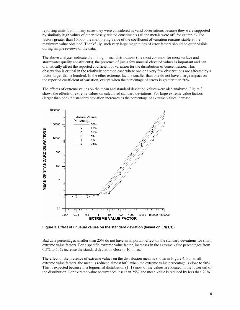
reporting units, but in many cases they were considered as valid observations because they were supported by similarly high values of other closely related constituents (all the metals were off, for example). For factors greater than 10,000, the multiplying value of the coefficient of variation remains stable at the maximum value obtained. Thankfully, such very large magnitudes of error factors should be quite visible during simple reviews of the data. The above analyses indicate that in lognormal distributions (the most common for most surface and stormwater quality constituents), the presence of just a few unusual elevated values is important and can dramatically affect the reported coefficient of variation for the distribution of concentration. This observation is critical in the relatively common case where one or a very few observations are affected by a factor larger than a hundred. In the other extreme, factors smaller than one do not have a large impact on the reported coefficient of variation, except when the percentage of errors is greater than 50%. The effects of extreme values on the mean and standard deviation values were also analyzed. Figure 3 shows the effects of extreme values on calculated standard deviations. For large extreme value factors (larger than one) the standard deviation increases as the percentage of extreme values increase.

Figure 3. Effect of unusual values on the standard deviation (based on LN(1,1)) Bad data percentages smaller than 25% do not have an important effect on the standard deviations for small extreme value factors. For a specific extreme value factor, increases in the extreme value percentages from 0.5% to 50% increase the standard deviation close to 10 times. The effect of the presence of extreme values on the distribution mean is shown in Figure 4. For small extreme value factors, the mean is reduced almost 80% when the extreme value percentage is close to 50%. This is expected because in a lognormal distribution (1, 1) most of the values are located in the lower tail of the distribution. For extreme value occurrences less than 25%, the mean value is reduced by less than 20%.

11

Large extreme value factors have much larger effects on the distribution means. As the extreme value percentage increases, the calculated means also increase. If 0.5% of the values are affected by a factor of a hundred, the mean value is doubled. If 50% of the values are affected by the same factor, the mean values are increased by almost 50 times. For factors larger than a thousand, increasing the percentages of extreme values from 0.5% to 50% increases the mean values by up to two orders of magnitude. These evaluations are important because it points out that for lognormal distributions, the effects of a few elevated values in the upper tail have a much greater effect on common statistics than unusual values in the lower tail. Many stormwater researchers have focused on the lower tail, especially when determining how to handle the detection limits and unreported data. Stormwater constituents usually have unusual values in both tails of the probability distribution. It is common to delete elevated values from the observations assuming they are expendable “outliers”. This practice is not recommended unless there is sufficient evidence that the observed values are a mistake. Actual elevated values can have a large effect on the calculated distribution parameters. If these are arbitrarily removed, the data analyses will likely be flawed.

Figure 4. Effect of unusual values on the mean (based on LN(1,1)) Examples of Methods used to Identify Corrupt Data When developing the NSQD, Maestre and Pitt (2005) obtained information from more than 70 communities concerning their NPDES Phase I monitoring activities. In cases where the data were submitted in electronic form, the data were manipulated with macros and stored in the main Excel spreadsheet database. For data from communities in paper form, the information was manually typed into the spreadsheet. Once the database was completed, the main table was first reviewed by rows (corresponding to individual runoff events) and then by columns (corresponding to measured constituents). Each row and column in the database was reviewed at least once and compared to information contained in the original reports (when available). For each constituent, probability plots, box and whisker plots, and time series plots were used to

12

identify possible errors (likely associated with the transcription of the information, or as typographical errors in the original reports). Most of the identified errors were attributed to the transcription process and, in some cases, errors during unit conversions (such as metal results reported as mg/L when they were really as µg/L). Additional “logical” plots were used to identify possible errors in the database. A plot of the dissolved (filtered) concentrations against the total concentrations for metals should indicate that the dissolved concentrations are lower than the total forms, for example (Figure 5). Other plots included TKN vs. NH3, COD vs. BOD5, SS vs. turbidity, and TDS vs. conductivity.

Figure 5. Example scatter plots of stormwater data (line of equivalent concentration shown) In all cases, suspect values were carefully reviewed and many were found to be associated with simple transcription errors, or obviously improper units, which could be corrected. However, about 300 suspect values (out of about 200,000 total data values) were removed from the database as they could not be verified. None of the data were deleted without sufficient evidence of a highly probable error. For example, if a set of samples from the same community had extremely high concentrations (in one case, 20 times larger than the typical concentrations reported for other events for the same community) at different sites, but for the same event, this will indicate a very likely error during the collection or analysis of the sample. If just a single site had high concentrations (especially if other related constituents were also high), it would not normally be targeted for deletion, but certainly subject to further scrutiny. If a value was deleted from the database, or otherwise modified, a question mark notation was assigned to the respective constituent in the qualifier column. A special list was retained that included all the modifications (changes and deletions) performed in the database.

13

Probability Distributions of Data Knowing the statistical distribution of the observed data is a critical step in data analysis. The selection of the correct statistical analyses tools is dependent on the data distribution, and many QA/QC operations depend on examining the distribution behavior. However, much data is needed for accurate determinations of the statistical distributions of the data, especially when examining unusual behavior. The comparison of probability distributions between different data subsets is also a fundamental method to identify important factors affecting data observations. Statistical analyses basically are intended to explain data variability by identifying significantly different subsets of the data. The remaining variability that can not be explained must be described. In all cases, accurate descriptions of the data probability distributions are needed. The Nationwide Urban Runoff Program (NURP) evaluated the characteristics of stormwater discharges at 81 outfalls in 28 communities throughout the U.S. (EPA 1983). One of the conclusions was that most of the stormwater constituent concentration probability plots could be described using lognormal distributions. More recently, Van Buren (1997) also found that stormwater concentrations were best described using a lognormal distribution for almost all constituents, with the exception of some dissolved constituents that were better described with a normal distribution. Beherra (2000) also found that some stormwater constituent concentrations were better described using a lognormal distribution, while others were better described with gamma or exponential distributions. The constituents that were best described with a gamma distribution included total solids, total Kjeldahl nitrogen (TKN), total phosphorous, chemical oxygen demand (COD), barium and copper. The constituents that were best described with an exponential distribution included suspended solids, nitrates and aluminum. In both of these recent studies, fewer than 50 samples (collected at the same site) were available for evaluation, so their wide applicability is uncertain. During the development of the NSQD, Maestre and Pitt (2005) used statistical tests to evaluate the log-normality of selected constituents of most interest in the database. Statistical descriptions were obtained of each set of data including box and whisker and probability plots for each land use category, and for the pooled dataset. It was found in almost all cases that the log-transformed data generally followed a straight line between the 5th and 95th percentile, as illustrated in Figure 6 for total dissolved solids (TDS) in residential areas. For many statistical tests focusing on the central tendency (such as for determining the average concentration that is used for mass balance calculations), this may be a suitable fit. As an example, WinSLAMM, the Source Loading and Management Model (Pitt and Voorhees 1995), uses a Monte Carlo component to describe the likely variability of stormwater source flow pollutant concentrations using either lognormal or normal probability distributions for each constituent. However, if the extreme values are of importance (such as when dealing with the influence of many non-detectable values on the predicted concentrations, or determining the frequency of observations exceeding a numerical standard that is close to either tail of the distribution), a better description of the extreme values may be important.

14

1 10 100 1000 10000Concentration (mg/L)

0.0050.01

0.02

0.05

0.1

0.2

0.30.40.50.6

0.7

0.8

0.9

0.95

0.98

0.990.995

0.9980.999

0.9995C

umul

ativ

e P

roba

bilit

y

LAND USEResidential

Probability Plot for Different Land Uses Total Dissolved Solids (mg/L)

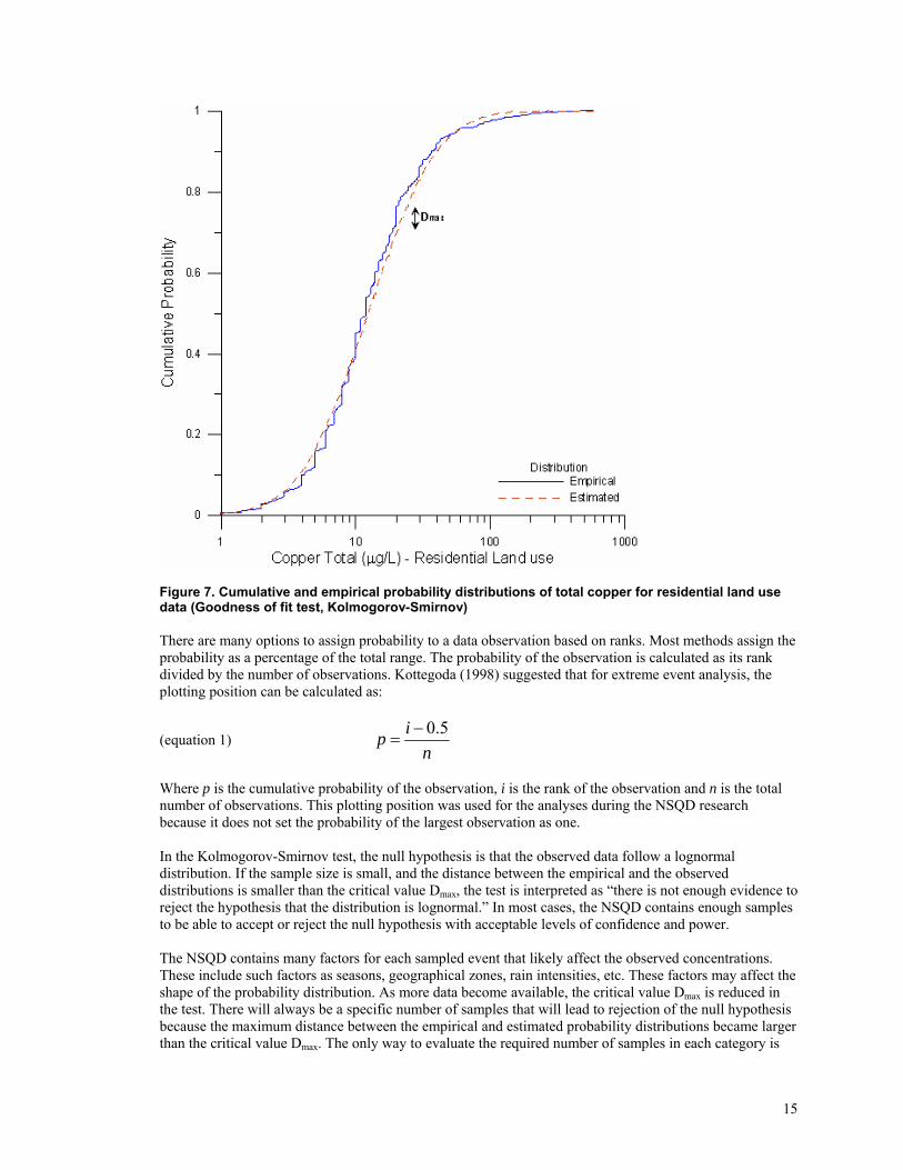
Figure 6. Log-probability plot of total dissolved solids in residential land use The NSQD underwent an extensive data evaluation process, including multiple comparisons of the all data values in the database to original documents. In some cases, data was available from the local agency in electronic form. These spreadsheets were reformatted to be consistent to the NSQD format. However, it was found that all of the submitted electronic data needed to be verified against original data sheets and reports. When reviewing the NSQD, it was assumed that some of the events in the upper and lower tails of the distributions were caused by errors, most likely due to faulty transcription of the data (such as mislabeling the units for heavy metals or nutrients as mg/L instead of µg/L, for example). Unusual values were verified with the original reports and datasets whenever possible. While some values (less than 5% of the complete dataset) were found to be in error and were corrected, most of the suspected values were found to be correct stormwater observations. Analysis of Log-normality of Stormwater Constituents Parameters The goodness of fit of twenty nine stormwater constituent probability distributions was evaluated using the Kolmogorov-Smirnov test. Figure 7 shows how the test accepts or rejects the null hypothesis that the empirical and the estimated distributions are the same. If the null hypothesis is valid, then the constituent can be adequately represented by the lognormal distribution. The observations are sorted and a probability is assigned by its rank. The distribution generated by this ranking is known as the empirical distribution. The estimated distribution function is also compared on the same plot. The estimated distribution function is calculated with the mean and standard deviation of the original data. If the distance between the empirical and the estimated distributions is higher than a critical value dα or Dmax, the hypothesis of lognormality is rejected. Notice in Figure 7 that the horizontal axis has a logarithmic scale.

15

Figure 7. Cumulative and empirical probability distributions of total copper for residential land use data (Goodness of fit test, Kolmogorov-Smirnov) There are many options to assign probability to a data observation based on ranks. Most methods assign the probability as a percentage of the total range. The probability of the observation is calculated as its rank divided by the number of observations. Kottegoda (1998) suggested that for extreme event analysis, the plotting position can be calculated as:

(equation 1) n

ip 5.0−=

Where p is the cumulative probability of the observation, i is the rank of the observation and n is the total number of observations. This plotting position was used for the analyses during the NSQD research because it does not set the probability of the largest observation as one. In the Kolmogorov-Smirnov test, the null hypothesis is that the observed data follow a lognormal distribution. If the sample size is small, and the distance between the empirical and the observed distributions is smaller than the critical value Dmax, the test is interpreted as “there is not enough evidence to reject the hypothesis that the distribution is lognormal.” In most cases, the NSQD contains enough samples to be able to accept or reject the null hypothesis with acceptable levels of confidence and power. The NSQD contains many factors for each sampled event that likely affect the observed concentrations. These include such factors as seasons, geographical zones, rain intensities, etc. These factors may affect the shape of the probability distribution. As more data become available, the critical value Dmax is reduced in the test. There will always be a specific number of samples that will lead to rejection of the null hypothesis because the maximum distance between the empirical and estimated probability distributions became larger than the critical value Dmax. The only way to evaluate the required number of samples in each category is

16

using the power of the test. Power is the probability that the test statistic will lead to a rejection of the null hypothesis when it is false (Gibbons and Chakraborti 2003). Masey (1950) states that the power of the Kolmogorov-Smirnov test can be written as: (equation 2)

{ }⎟⎟⎠

⎞⎜⎜⎝

⎛

−∆±

<−

−<

−∆±−

−=))(1)(())(1)((

)()())(1)((

Pr101010101

010

0101 xFxFnd

xFxFnxFxS

xFxFndpower n αα

where: dα = Dmax: critical distance at the level of significance α (confidence of the test), Sn = Cumulative empirical probability distribution, F1 = Cumulative alternative probability distribution, ∆ = Maximum absolute difference between the cumulative estimated probability distribution and the alternative cumulative probability distribution. Massey (1951) also found that for large sample sizes, the power can be never be smaller than

(equation 3) ∫+∆

−∆

−−>

)(2

)(2

2

2

211

ndn

ndn

t

dtepowerα

απ

This reduced expression can be used to calculate the number of samples required to reject the null hypothesis with a desired power. Figure 8 shows the power of the D test for 1%, 5%, and 10% levels of confidence of the test for sample sizes larger than 35 (Massey 1951). For example, assume that the maximum distance between the alternative cumulative and the estimated cumulative probability distributions is 0.2, and we want an 80% power (0.8) against the alternative at a 5% level of confidence. To calculate the number of required samples, we read that ∆(N)0.5 is 1.8 for a power of 0.8 and 5% level of confidence. Solving for N = (1.8/0.2)² = 81 samples. If we want to calculate the number of samples when the difference between the alternative cumulative and the estimated cumulative probability function is 0.05, with the same power and level of confidence, then 1,296 samples would be required. When the lines are very close together, it is obviously very difficult to statistically show that they are different, and many samples are needed.

17

Figure 8. Lower bounds for the power of the D test for α = 1%, 5% and 10% (N>35)

The Kolmogorov-Smirnov test was used to indicate if the cumulative empirical probability distribution of the NSQD residential stormwater constituents can be adequately represented with a lognormal distribution. Table 2 shows the resulting power of the test for D=0.05 and D=0.1, when applied to selected constituents that had high levels of detection in residential land uses. Table 2. Power of the Test When Applied to Selected Constituents in Residential Land Uses

Constituent N Percentage Detected

∆N0.5

(α=0.05) Power

(D=0.05, β=5%)

∆N0.5

(α=0.1) Power (D=0.1, β =10%)

TDS (mg/L) 861 99.2 1.46 0.60 2.92 1 TSS (mg/L) 991 98.6 1.56 0.65 3.12 1 BOD (mg/L) 941 97.6 1.52 0.65 3.04 1 COD (mg/L) 796 98.9 1.40 0.55 2.80 1 NO2+NO3 (mg/L) 927 97.4 1.50 0.60 3.00 1 TKN (mg/L) 957 96.8 1.52 0.65 3.04 1 TP (mg/L) 963 96.9 1.53 0.65 3.06 1 Total Copper (µg/L) 799 83.6 1.29 0.50 2.58 1 Total Lead (µg/L) 788 71.3 1.19 0.40 2.38 1 Total Zinc (µg/L) 810 96.4 1.40 0.55 2.80 1

Table 2 shows that the number of collected samples is sufficient to detect if the empirical distribution is located inside an interval of width 0.1 above and below the estimated cumulative probability distribution. If the interval is reduced to 0.05, the power varies between 40 and 65%. To estimate the interval width, 10 cumulative distributions of 1,000 random data points, having a lognormal (1, 1) distribution, were compared with the estimated cumulative distribution for normal, gamma and exponential distributions. The maximum distance between the cumulative lognormal and the cumulative normal distributions was 0.25. The maximum distance with cumulative gamma (the same for exponential in this case) was 0.28. An interval width of 0.1 was considered appropriate for the analysis.

18

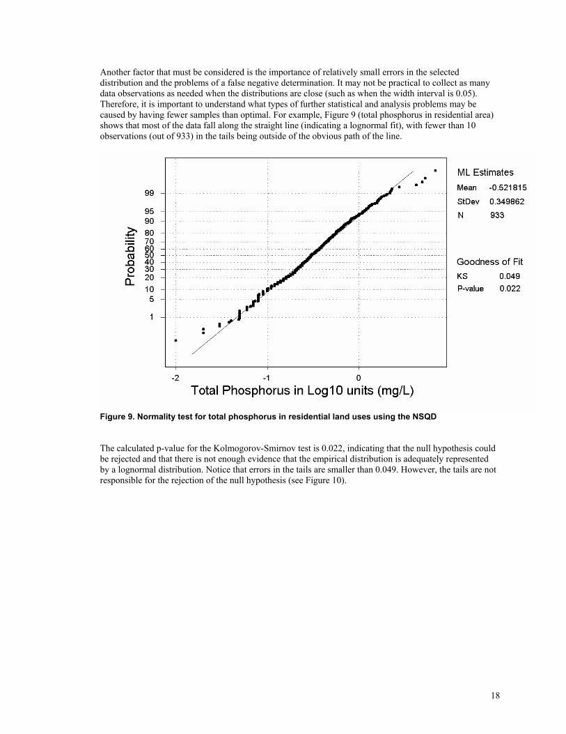
Another factor that must be considered is the importance of relatively small errors in the selected distribution and the problems of a false negative determination. It may not be practical to collect as many data observations as needed when the distributions are close (such as when the width interval is 0.05). Therefore, it is important to understand what types of further statistical and analysis problems may be caused by having fewer samples than optimal. For example, Figure 9 (total phosphorus in residential area) shows that most of the data fall along the straight line (indicating a lognormal fit), with fewer than 10 observations (out of 933) in the tails being outside of the obvious path of the line.

Figure 9. Normality test for total phosphorus in residential land uses using the NSQD

The calculated p-value for the Kolmogorov-Smirnov test is 0.022, indicating that the null hypothesis could be rejected and that there is not enough evidence that the empirical distribution is adequately represented by a lognormal distribution. Notice that errors in the tails are smaller than 0.049. However, the tails are not responsible for the rejection of the null hypothesis (see Figure 10).

19

Figure 10. Dmax was located in the middle of the distribution

In this case, Dmax is located close to a total phosphorus concentration of 0.2 mg/L (-0.7 in log scale). As in this case, the hypothesized distributions are usually rejected because of the departures in the middle of the distribution, not in the tails (the vertical distances between the two curves are larger). However, as previously pointed out, a small number of observations in the upper tail can change the shape of the estimated cumulative probability distribution by affecting the mean and standard deviation of the data. The methods used previously by Van Buren and Beherra evaluated the probability distributions only using two parameters, the median and the standard deviation. They suggested the gamma and exponential distributions as alternatives to the lognormal for some stormwater constituents. For residential, commercial and industrial land uses, the lognormal distribution was found to best fit the empirical data, except for selenium and silver in commercial land uses. In open space land uses, about 50% of the constituents were adequately fitted by the lognormal distribution, 30% by the gamma distribution and the remaining by the exponential distribution. In freeway areas, lognormal distributions better fit most of the constituents, except that fecal streptococcus, total arsenic and total chromium were better fitted by the gamma distribution and ammonia was better fitted by the exponential distribution. Residential, commercial and industrial land uses had larger sample sizes than the other two land uses. It seems that for small sample sizes, gamma and exponential distributions better represent actual stormwater constituent distributions, but once the number of samples increase, the lognormal distribution is best. The few cases where the gamma distribution was a better fit were for NO2+NO3 in industrial land uses, and chromium in freeway areas. The exponential distribution better represents total ammonia in freeway areas (with around 70 detected samples) than the other two distribution types. Other transformations were also tested, such as the square root, and other power functions, but the results were not improved. It was therefore decided to investigate if a three-parameter lognormal distribution function can be used to improve the overall goodness of fit for stormwater constituent probability distributions. As shown in the following discussion, this third parameter, in some cases, allows a much better fit of the cumulative empirical and estimated probability distributions. Goodness of fit was evaluated using a 3-parameter lognormal probability distribution. The probability distributions were created for residential, commercial, industrial, open space and freeways land uses. The

20

distribution parameters were calculated using the maximum likelihood and the L-moments methods. The maximum likelihood method requires that it be solved iteratively using three equations. The results were compared with the 2-parameter standard model and the actual data. The model with the smaller maximum distance between the empirical and the estimated function was selected as the best model. All the calculations were made using only the detected values. In general, the L-moments method provided a better fit for the upper tail of the distribution whereas the maximum likelihood method provided a better fit for the lower tail. Figure 11 shows the three estimated models for TSS in commercial land use areas.

Figure 11. Estimated models for TSS in commercial land uses In this graph, it is observed that the empirical distribution has higher concentrations in the upper tail compared with any of the three models. In the lower tail, the maximum likelihood method using the 3-parameters better fit the observed values. In this case, the maximum likelihood method was better than the other two models, although none of the methods adequately represented the extreme high values. The L-moments method generally betters fits the upper tail distribution, but typically trims or overestimates the lower tail. Figure 12 shows the results for TDS in industrial land uses. The L-moments better fits the empirical distribution in the upper tail, but it trims any observation smaller than 35 mg/L (almost 20% of the total dataset) in the lower tail. The 2-parameter lognormal and the maximum likelihood method provide better results, although both were worse than the L-moments in the upper tail region.

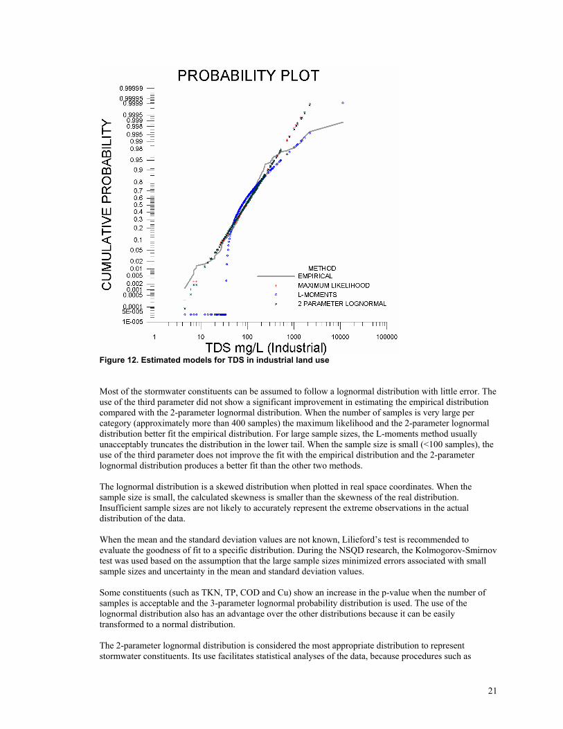
21

Figure 12. Estimated models for TDS in industrial land use Most of the stormwater constituents can be assumed to follow a lognormal distribution with little error. The use of the third parameter did not show a significant improvement in estimating the empirical distribution compared with the 2-parameter lognormal distribution. When the number of samples is very large per category (approximately more than 400 samples) the maximum likelihood and the 2-parameter lognormal distribution better fit the empirical distribution. For large sample sizes, the L-moments method usually unacceptably truncates the distribution in the lower tail. When the sample size is small (<100 samples), the use of the third parameter does not improve the fit with the empirical distribution and the 2-parameter lognormal distribution produces a better fit than the other two methods. The lognormal distribution is a skewed distribution when plotted in real space coordinates. When the sample size is small, the calculated skewness is smaller than the skewness of the real distribution. Insufficient sample sizes are not likely to accurately represent the extreme observations in the actual distribution of the data. When the mean and the standard deviation values are not known, Lilieford’s test is recommended to evaluate the goodness of fit to a specific distribution. During the NSQD research, the Kolmogorov-Smirnov test was used based on the assumption that the large sample sizes minimized errors associated with small sample sizes and uncertainty in the mean and standard deviation values. Some constituents (such as TKN, TP, COD and Cu) show an increase in the p-value when the number of samples is acceptable and the 3-parameter lognormal probability distribution is used. The use of the lognormal distribution also has an advantage over the other distributions because it can be easily transformed to a normal distribution. The 2-parameter lognormal distribution is considered the most appropriate distribution to represent stormwater constituents. Its use facilitates statistical analyses of the data, because procedures such as

22

ANOVA or regression require the errors to be normally distributed. If the number of observations is small, the use of nonparametric methods will be required, as the distributions cannot be accurately determined. Some nonparametric methods require symmetry in the data distribution. The log transformed constituent concentrations usually satisfy these assumptions. Identification of Unusual Monitoring Locations using Xbar and S Charts The following example illustrates the steps used to identify unusual sampling locations in the NSQD database (Maestre and Pitt 2005). This analysis was performed in three steps. First, box and whisker plots we used to identify any site with concentrations unusually high or low compared with the other residential locations. The plots were used to identify differences between and within EPA Rain Zones. Figure 13 shows that there are some sites in EPA Rain Zone 2 having lower TSS concentrations than the remaining residential sites included in the database. On the other hand, it seems that sites located in EPA Rain Zone 4 have higher concentrations than other groups. The second step was to identify those single residential sites that failed the Xbar and S chart tests for all the observations and by EPA Rain Zone. An Xbar chart shows the sample means, while S charts show the standard deviations of all samples within control limits. The control limits are calculated based on the number of samples collected at each site and show when individual sites are “out of bounds.” Normally, 95 percent confidence limits are plotted, so it is expected that about 5% of the sites will be outside the limits. An indication of geographical differences is if the Xbar chart using all observations shows clusters close or outside the control limits. The effect will be confirmed if none of the sites failed the Xbar test within EPA Rain Zones. The S chart identifies those sites that have a larger or smaller variation than the overall sites in the set. Figure 14 shows the Xbar and S chart for the residential land use sites. Six sites have mean TSS values different from the remaining sites in the same group. One important characteristic of this plot is that the control limits change with the number of samples collected at each site. The S chart identifies those sites with standard deviations different than the pooled deviation of the data set. In this case, two sites are outside the control limits. Table 3 shows the sites that failed the Xbar and S chart for all residential sites and for each EPA Rain Zone.

23

EPA Rain Zone and Location_ID

Tota

l Sus

pend

ed S

olid

s m

g/L

9_CO

DEA0

059_

CODE

A003

8_ID

ADA0

027_

ORS

AA00

47_

ORP

OA0

067_

ORG

RA00

37_

ORE

UA00

37_

ORC

CA00

47_

ORC

CA00

37_

ORC

CA00

27_

ORC

CA00

16_

AZTU

A002

6_AZ

TUA0

016_

AZM

CA00

65_

TXM

EA00

35_

TXM

EA00

25_

TXIR

A001

5_TX

DAA0

055_

TXAR

A003

5_TX

ARA0

024_

TXHO

A005

4_TX

HOA0

034_

TXHC

A006

4_KA

WIH

UNT

4_KA

TOBR

OO

4_KA

TOAT

WO

3_GA

COC1

A33_

GACL

COTR

3_GA

ATAT

023_

ALM

OSI

VI3_

ALM

OSA

RA3_

ALM

OCR

EO3_

ALJC

C009

3_AL

HUHU

RI3_

ALHU

DRAV

2_VA

VBTY

V22_

VAVB

TYV1

2_VA

PMTY

P52_

VAPM

TYP4

2_VA

PMTY

P22_

VANN

TNN1

2_VA

NFTY

N52_

VANF

TYN3

2_VA

NFTY

N22_

VAHC

COR2

2_VA

HCCO

R12_

VAHA

TYH5

2_VA

HATY

H42_

VAHA

TYH3

2_VA

FFCO

F52_

VAFF

COF3

2_VA

FFCO

F12_

VACP

TYC3

2_VA

CPTY

C12_

VACP

TC1A

2_VA

CHCO

F52_

VACH

COF3

2_VA

CHCN

2A2_

VACH

CN1A

2_VA

CHCC

C52_

VAAR

LLP1

2_VA

ARLC

V22_

TNM

ET41

02_

TNM

ET23

12_

PAPH

1014

2_PA

PH08

912_

PAPH

0864

2_NC

GRW

ILL

2_NC

GRRA

ND2_

NCFV

TRYO

2_NC

FVCL

EA2_

NCCH

SIM

S2_

NCCH

NANC

2_NC

CHHI

DD2_

MDS

HDTP

S2_

MDP

GCO

S42_

MDP

GCO

S22_

MDM

OCO

QA

2_M

DMO

CONV

2_M

DHO

COM

H2_

MDH

OCO

GM2_

MDH

ACO

BP2_

MDC

LCO

CE2_

MDB

CTYH

R2_

MDB

CTYH

O2_

MDB

ACO

WC

2_M

DBAC

OSC

2_M

DAAC

ORK

2_M

DAAC

OO

D2_

KYLX

TBL1

2_KY

LXNE

L12_

KYLX

EHL7

2_KY

LOTS

R32_

KYLO

TSR1

1_M

NMIS

D02

1_M

NMIS

D01

1_M

ABO

A006

1_M

ABO

A002

-

1.000

-

100

-

10

-

1-2 2-3 3-41-2 2-3 4-5 5-6 6-7 78 9

Boxplot of TSS in Residential Land Uses

Figure 13. TSS box plots in residential land use by EPA Rain Zone and location

24

Sample

To

tal

Su

spe

nd

ed

So

lid

s m

g/L

554943373125191371

-

100

-

10

-

__X= 41.88UC L= 70.63

LC L= 24.77

Sample

Sa

mp

le S

tDe

v (

Lo

g)

554943373125191371

1.00

0.75

0.50

0.25

0.00

_S=0.404

UC L=0.567

LC L=0.242

1

1

11

11

1

1

Xbar-S Chart of TSS in Residential Land Use - EPA Rain Zone

Figure 14. Xbar S chart for residential land use in EPA Rain Zone 2

Table 3. Sites Failing Xbar and R Chart in Residential Land Uses

Rain Zone Sites Failing Xbar chart Sites Failing S Chart

ALL

AZTUA001(H) CODEA005(H) GAATAT02(L) GACLCOTR(H) KATOATWO(H) KATOBROO(H) KYLXEHL7(L) MDPGCOS2(H) MNMISD01(H) NCCHSIMS(L) NCFVCLEA(L) NCFVTRYO(L) NCGRWILL(L) ORCCA004(L) TXHCA006(H) TXHOA003(L) VAARLCV2(L) VAARLLP1(L) VACHCOF3(L) VACHCOF5(L) VAHATYH5(L) VAPMTYP5(L)

VAVBTYV2(L)

1 None None

2 MDPGCOS2(H) MDSHDTPS(H) NCCHSIMS(L) VACHCOF3(L) VACHCOF5(L) VAVBTYV1(H)

MDSHDTPS(H) VAVBTYV2(L)

3 GACLCOTR(H) None 4 TXHCA006(H) TXHOA003(L) None 5 None None 6 None None 7 None None 8 None None 9 None None

Table 3 shows that most of the sites located below the lower control limit were located in North Carolina, Virginia (EPA Rain Zone 2) or Oregon (EPA Rain Zone 7). Sites above the upper control limit were located in Arizona (EPA Rain Zone 6), Kansas (EPA Rain Zone 4), and Colorado (EPA Rain Zone 9).

25

Xbar plots by EPA Rain Zones also indicate differences within groups. EPA Rain Zones 2, 3, and 4 showed nine sites failing the Xbar test. Six sites out of 54 failed the Xbar chart test in residential land use EPA Rain Zone 2. Each of these sites were examined individually to identify usually site conditions that may explain the unusual observed concentrations. The final step used ANOVA to evaluate if any EPA Rain Zone was different than the others. The ANOVA table indicated a p-value close to zero, indicating that there are significant differences in the TSS concentration among at least two of the different EPA Rain Zones. The Dunnett’s comparison test with a family error of 5% indicate that concentrations in EPA Rain Zones 4 (median TSS= 91 mg/L), 5 (median TSS = 83 mg/L), 6 (median TSS=118 mg/L), 7 (median TSS = 69 mg/L), and 9 (median TSS = 166 mg/L) are significantly higher than the concentrations observed in EPA Rain Zone 2 (median TSS = 49 mg/L). This same procedure was performed for the following 13 additional constituents in residential, commercial and industrial land use areas: hardness, TSS, TDS, oil and grease, BOD, COD, NO2 + NO3, ammonia, TKN, dissolved phosphorus, total phosphorus, copper, lead and zinc. Identifying the Needed Detection Limits and Selecting the Appropriate Analytical Method The selection of the analytical procedure is dependent on a number of factors, including (in order of general importance):

• appropriate detection limits • freedom from interferences • good analytical precision (repeatability) • minimal cost • reasonable operator training, needed expertise, disposal of used reagents and safety of the method (a great concern when volunteers are used to conduct the monitoring program).

One of the most critical and obvious determinants used for selecting an appropriate analytical method is the identification of the needed analytical detection limit. It is possible to select available analytical methods that have extremely low detection limits. Unfortunately, these very sensitive methods are typically costly and difficult to utilize. However, in many cases, these extremely sensitive methods are not needed. The basic method of selecting an appropriate analytical method is to ensure that it can identify samples that exceed appropriate criteria for the parameter being measured. If detection limits are smaller than a critical water quality criterion or standard, then analytical results that may indicate interference with a beneficial use can be directly selected. Burton and Pitt (2002) summarize water quality criteria for many constituents of concern in receiving water studies and describe typical levels of performance for different analytical methods. The following discussion summarizes some of this information. Environmental researchers need to be concerned with many attributes of numerous analytical methods when selecting the most appropriate methods to use for analyses of their samples. Besides the factors listed above, another consideration is whether the analyses should/can be conducted in the field, or in the laboratory. These factors can be grouped into many categories including:

• capital cost, costs of consumables, training costs, method development costs, age before obsolesce, age when needed repair parts or maintenance supplies are no longer available, replacement costs, other support costs (data management, building and laboratory requirements, waste disposal, etc.).

• sensitivity, interferences, selectivity, repeatability, quality control and quality assurance reporting, etc. • sample collection, preservation, and transportation requirements, etc. • long-term chemical exposure hazards, waste disposal hazards, chemical storage requirements, etc. Most of these issues are not well documented in the literature for environmental sample analyses. Aspects of analytical reliability have received the most attention in the literature, but most of the other aspects noted above have

26

not been adequately discussed for the many analytical alternatives available, especially for field analytical methods. It is therefore difficult for a water quality analyst to decide which methods to select, or even if a choice exists. The selection of the appropriate analysis procedure is dependent on the use of the data and how false negatives or false positives would affect water use decisions or regulatory questions. The QA objectives for the method detection limit (MDL) and precision (RPD) for the compounds of interest are a function of the anticipated median concentrations in the samples. The MDL objectives should generally be about 0.25, or less, of the median value for sample sets having typical concentration variations (COV values ranging from 0.5 to 1.25), based on many Monte Carlo evaluations to examine the rates of false negatives and false positives. The precision goal is estimated to be in the range of 10 to 100% (Relative Percent Difference of duplicate analyses), depending on the sample variability. Table 4 lists the typical median stormwater runoff constituent concentrations and the associated calculated MDL and RPD goals, for a typical stormwater monitoring project. There are several different detection limits that are used in laboratory analyses. Standard Methods (1995) states that the common definition of a detection limit is that it is the smallest concentration that can be detected above background noise, using a specific procedure and with a specific confidence. The instrument detection limit (IDL) is the concentration that produces a signal that is three standard deviations of the noise level. This would result in about a 99% confidence that the signal was different from the background noise. This is the simplest measure of detection and is solely a function of the instrument and is not dependent on sample preparation. The method detection limit (MDL) accounts for sample preparation in addition to the instrument sensitivity. The MDL is about four times greater than the IDL because sample preparation increases the variability in the analytical results. Automated methods have MDLs much closer to the IDLs than manual sample preparation methods. An MDL is determined by spiking reagent water with a known concentration of the analyte of interest at a concentration close to the expected MDL. Seven portions of this solution are then analyzed (with complete sample preparation) and the standard deviation is calculated. The MDL is 3.14 times this measured standard deviation (at the 99% confidence level). The practical quantification limit (PQL) is a more conservative detection limit and considers the variability between laboratories using the same methods on a routine basis. The PQL is estimated in Standard Methods to be about five times the MDL. Log-normal probability distributions are commonly used to describe the concentration distributions of water quality data, including stormwater data (EPA 1983). The data ranging from the 10th to the 90th percentile typically can be suitably described as a log-normal probability distribution. However, values less than the 10th percentile value are usually less than predicted from the log-normal probability plot, while values greater than the 90th percentile value are usually greater than predicted from the log-normal probability plot. The range-ratio can generally be easily selected based on the expected concentrations to be encountered, ignoring the most extreme values. As the range ratio increases, the COV also increases, up to a maximum value of about 2.5 for the set of conditions studied by Pitt and Lalor 2000. Pitt and Lalor (2000) conducted numerous Monte Carlo analyses using mixtures having broad ranges of concentrations. Using these data, they developed guidelines for estimating the needed detection limits to characterize water samples. If the analyte has an expected narrow range of concentrations (a low COV), then the detection limit can be greater than if the analyte has a wider range of expected concentrations (a high COV). These guidelines are as follows:

• If the analyte has a low level of variation (a 90th to 10th percentile range ratio of 1.5, or a COV of <0.5), then the estimated required detection limit is about 0.8 times the expected median concentration. • If the analyte has a medium level of variation (a 90th to 10th percentile range ratio of 10, or a COV of about 0.5 to 1.25), then the estimated required detection limit is about 0.23 times the expected median concentration. • Finally, if the analyte has a high level of variation (a 90th to 10th percentile range ratio of 100, or a COV of about >1.25), then the estimated required detection limit is about 0.12 times the expected median concentration.

27

Table 4. Summary of Quantitative QA Objectives (MDL and RPD) Required for an Example Stormwater Characterizaton Project

Constituent Units Example

COV category1

Example Median Conc.

Calculated MDL Requirement

Calculated RPD Requirement

pH pH units very low 7.5 must be readable

to within 0.3 unit <0.3 unit

specific conductance µmhos/cm low 100 80 <10% hardness mg/L as

CaCO3 low 50 40 <10%

Color HACH units low 30 24 <10% Turbidity NTU low 5 4 <10% COD mg/L medium 50 12 <30% suspended solids mg/L medium 50 12 <30% Particle size size

distribution medium 30 µm 7 µm <30%

alkalinity mg/L as CaCO3

low 35 30 <10%

chloride mg/L low 2 1.5 <10% nitrates mg/L low 5 4 <10% sulfate mg/L low 20 16 <10% calcium mg/L low 20 16 <10% magnesium mg/L low 2 1.5 <10% sodium mg/L low 2 1.5 <10% potassium mg/L low 2 1.5 <10% Microtox™ toxicity screening

I20 or EC50 medium I20 of 25% I20 of 6% <30%

chromium µg/L medium 40 9 <30% copper µg/L medium 25 6 <30% lead µg/L medium 30 7 <30% nickel µg/L medium 30 7 <30% zinc µg/L medium 50 12 <30% 1,3-dichlorobenzene µg/L medium 10 2 <30% benzo(a) anthracene µg/L medium 30 8 <30% bis(2-ethylhexyl) phthalate µg/L medium 20 5 <30% butyl benzyl phthalate µg/L medium 15 3 <30% fluoranthene µg/L medium 15 3 <30% pentachlorophenol µg/L medium 10 2 <30% phenanthrene µg/L medium 10 2 <30% pyrene µg/L medium 20 5 <30% Lindane µg/L medium 1 0.2 <30% Chlordane µg/L medium 1 0.2 <30%

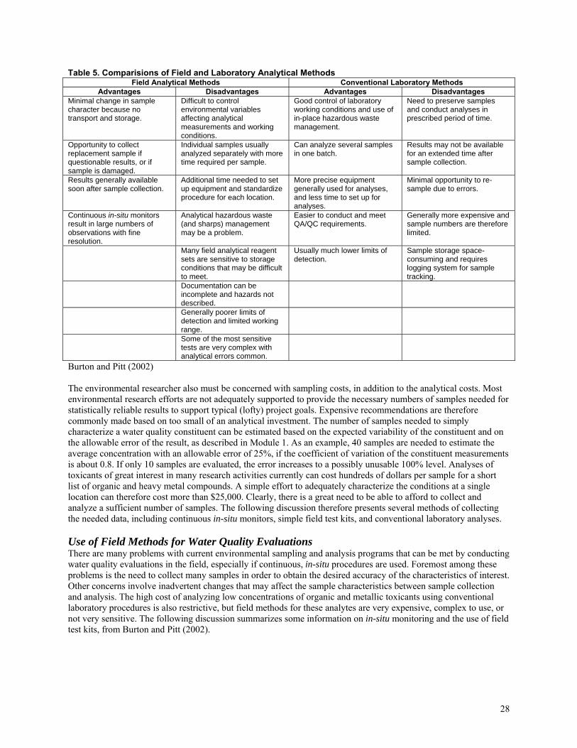
1 COV value: Multiplier for MDL: RDL Objective: <0.5 (low) 0.8 <10% 0.5 to 1.25 (medium) 0.23 <30% >1.25 (high) 0.12 <50% from: Pitt and Lalor 1998 In some cases, field test kits, or especially continuous in-situ monitors, may be prefereable over conventional laboratory methods. Table 5 (Burton and Pitt 2002) lists some of the benefits and problems associated with each general approach. The advantages of field analytical methods can be very important; however their limitations must be recognized and considered.

28

Table 5. Comparisions of Field and Laboratory Analytical Methods Field Analytical Methods Conventional Laboratory Methods

Advantages Disadvantages Advantages Disadvantages Minimal change in sample character because no transport and storage.

Difficult to control environmental variables affecting analytical measurements and working conditions.

Good control of laboratory working conditions and use of in-place hazardous waste management.

Need to preserve samples and conduct analyses in prescribed period of time.

Opportunity to collect replacement sample if questionable results, or if sample is damaged.

Individual samples usually analyzed separately with more time required per sample.

Can analyze several samples in one batch.

Results may not be available for an extended time after sample collection.

Results generally available soon after sample collection.

Additional time needed to set up equipment and standardize procedure for each location.

More precise equipment generally used for analyses, and less time to set up for analyses.

Minimal opportunity to re-sample due to errors.

Continuous in-situ monitors result in large numbers of observations with fine resolution.

Analytical hazardous waste (and sharps) management may be a problem.

Easier to conduct and meet QA/QC requirements.

Generally more expensive and sample numbers are therefore limited.

Many field analytical reagent sets are sensitive to storage conditions that may be difficult to meet.

Usually much lower limits of detection.

Sample storage space-consuming and requires logging system for sample tracking.

Documentation can be incomplete and hazards not described.

Generally poorer limits of detection and limited working range.

Some of the most sensitive tests are very complex with analytical errors common.

Burton and Pitt (2002) The environmental researcher also must be concerned with sampling costs, in addition to the analytical costs. Most environmental research efforts are not adequately supported to provide the necessary numbers of samples needed for statistically reliable results to support typical (lofty) project goals. Expensive recommendations are therefore commonly made based on too small of an analytical investment. The number of samples needed to simply characterize a water quality constituent can be estimated based on the expected variability of the constituent and on the allowable error of the result, as described in Module 1. As an example, 40 samples are needed to estimate the average concentration with an allowable error of 25%, if the coefficient of variation of the constituent measurements is about 0.8. If only 10 samples are evaluated, the error increases to a possibly unusable 100% level. Analyses of toxicants of great interest in many research activities currently can cost hundreds of dollars per sample for a short list of organic and heavy metal compounds. A simple effort to adequately characterize the conditions at a single location can therefore cost more than $25,000. Clearly, there is a great need to be able to afford to collect and analyze a sufficient number of samples. The following discussion therefore presents several methods of collecting the needed data, including continuous in-situ monitors, simple field test kits, and conventional laboratory analyses. Use of Field Methods for Water Quality Evaluations There are many problems with current environmental sampling and analysis programs that can be met by conducting water quality evaluations in the field, especially if continuous, in-situ procedures are used. Foremost among these problems is the need to collect many samples in order to obtain the desired accuracy of the characteristics of interest. Other concerns involve inadvertent changes that may affect the sample characteristics between sample collection and analysis. The high cost of analyzing low concentrations of organic and metallic toxicants using conventional laboratory procedures is also restrictive, but field methods for these analytes are very expensive, complex to use, or not very sensitive. The following discussion summarizes some information on in-situ monitoring and the use of field test kits, from Burton and Pitt (2002).

29

Continuously Recording and Long-Term In-Situ Measurements of Water Quality Parameters. Several classical instruments have long been available to measure various water quality parameters with unattended instruments for relatively long periods of time. Hydrolab and YSI have offered equipment that could monitor dissolved oxygen, pH, temperature, and conductivity unattended for several decades, with more vendors entering the market. The early instruments were plagued with stability problems and were usually most suited for unattended operation over a period of only about a day. This was still a major break-through, as it enabled diurnal fluctuations of these important parameters to be accurately and relatively conveniently obtained. Currently available equipment, in contrast, has been demonstrated to be capable of unattended operations for longer than a month. These are relatively expensive instruments that can cost up to $7,000 each, depending on options selected. Examples of equipment currently available include the 803 probe series from Solomat which can have up to 8 sensors installed. These may include pH, ORP, DO, temperature, conductivity, depth, ammonium, nitrite, and other ions by ISE. Several meters and data loggers are available for hand-held real-time measurements, or for long-term unattended operation. Unfortunately, the automated ISE analyses (nutrients, for example) are not yet very useful for stormwater conditions due to poor stability and comparisons with standard analyses methods. YSI also offers several in-situ probe instruments. The current 6000 series sonde is self-contained, measuring and logging up to 9 separate parameters simultaneously, including DO, conductivity, temperature, pH, depth, ORP, nitrate, ammonium, and turbidity. The rapid pulse DO and self-wiping turbidity sensors enable very long unattended operations (up to 45 days), with minimal fouling or drift. Hazco (800-332-0435) sells the YSI 6000 basic sonde (catalogue # B-6001) for about $7,000. The unit without the depth sensor is about $500 less. The performance specifications for the more common sensors, provided by YSI, are given in Table 6. Burton and Pitt (2002) contains detailed instructions for calibrating and setting up the sondes.

30

Table 6. YSI6000 specifications. Parameter Sensor Type Range Accuracy Resolution Dissolved Oxygen % saturation

Rapid Pulse — Clark-type, polarographic

0 to 200% air saturation

± 2% air saturation 0.1% air saturation

Conductivity* 4 electrode cell with autoranging

0 to 100 mS/cm ±0.5% of reading + 0.001 mS/cm

0.01 mS/cm

Temperature

Thermistor -5 to 45o C ± 0.15o C 0.01o C

pH Glass combination electrode

2 to 14 units ± 0.2 units 0.01 units

ORP Platinum ring -999 to 999 mV ± 20 mV 0.1 mV

Turbidity Optical, 90o scatter, mechanical cleaning

0 to 1000 NTU ± 5% 0.1 NTU

Depth — Medium Stainless steel strain guage

0 to 61 m ±0.12 m 0.001 m

Depth — Shallow Stainless steel strain guage

0 to 9.1 m ± 0.06 m 0.001 m

* Report outputs of specific conductance (conductivity corrected to 25o C) These unattended instruments are capable of collecting high resolution data (typically with observations every 15 minutes) over long periods. This is extremely useful in receiving water studies affected by stormwater. Even though few dissolved oxygen problems have ever been associated with stormwater (in contrast to CSOs), these probes are unexcelled in documenting the exposure periods and gross variations in receiving water conditions over many separate storm events. This data is very important when used in conjunction with in-situ toxicity test chambers that are exposed for relatively long periods of time. In addition, the YSI self-contained probes with rapid-pulse DO sensors (the probes consume very little power and oxygen themselves) can be used in light and dark chambers to conveniently obtain necessary data pertaining to sediment and water photosynthesis and respiration. Figure 15 is an example of a YSI 6000 output of high-resolution data for turbidity for a stormwater treatment device (the UpFloTM Filter) during an actual storm event, showing the very high turbidity levels at the beginning of the event in the influent, with much reduced turbidity in the treated effluent (Pitt and Khambhammettu 2006).

0

200

400

600

800

1000

1200

1400

3/26/2005 18:00

3/26/2005 19:12

3/26/2005 20:24

3/26/2005 21:36

3/26/2005 22:48

3/27/2005 0:00

Date/Time

Turb

idity

(NTU

)

Figure 15. Comparison of Turbidity for Storm Event on March 26, 2005 (Pitt and Khambhammettu 2006).

31

Field Test Kits Field test kits cover a wide range of instrumentation and methods. They range from very simple visual comparator tests (which use colored paper, colored solutions in small vials, or color wheels, to match against the color developed with the test) to miniaturizations of standard laboratory tests (using small spectrophotometers or other specialized instruments). Burton and Pitt (2002) also contains detailed performance information and descriptions for many field test kits, highlighting their performance (limits of detection, repeatability, and recovery), hazards associated with their use, complications and time requirements, approximate costs, and other notes. The least expensive test kits use small droppers or spoons to measure reagents into a reaction tube where the color is developed. More sophisticated tests use small filter colorimeters to more precisely measure the color developed during the test. HACH also offers continuous wavelength field spectrophotometers that are capable of measuring a wide variety of chemical parameters using a single instrument. La Motte has a filter colorimeter that contains several filter sets, also enabling many different chemical analyses to be conducted with the one instrument. HACH also has a field titration kit that is also very flexible providing additional capabilities that are not available with spectrophotometric methods. These multi-parameter instruments are usually superior to the simple dedicated test kits because of the increased sensitivity and precision that is achievable with the better equipment. They of course cost more. If only one or two parameters are to be monitored in the field, then it may be hard to justify the added cost of the more flexible instruments. However, if the best quality data is needed, then the cost may be justified, especially if more than a few parameters are to be measured. Also included in the category of field test kits are very sophisticated methods that are laboratory instrumentation and procedures that have been miniaturized and simplified. Some of these tests even meet the EPA reporting requirements for NPDES permit compliance. However, some of the field procedures skip certain sample clean-up or digestion steps that would be impractical to conduct in the field and are therefore not suitable for compliance monitoring. It is important to check with the field equipment suppliers and the reviewing regulatory agency to verify the current status of a field method for various reporting purposes. Many of the spectrophotometer and titration methods fall into this category of simplified laboratory methods. Several instruments are also available that permit sensitive and precise heavy metal (especially copper and lead) analyses in the field. However, these instruments are expensive (equipment costs of $2,000 to $4,000 and per sample costs of $5 to $15). They are also not sensitive to particulate-bound metals (which may be an advantage, depending on study objectives). The biggest difficulty with almost all of these field test kits is that they can require a substantial amount of time to evaluate the water sample, especially when only one sample at a time is being analyzed. Continuous and in-situ monitors eliminate field analytical time. Even though these field test kits enable personnel to evaluate samples at the point of collection, that may not be desirable. Lalor (1993), Pitt, et al. (1994), and more recently CWP and Pitt (2004) found that test kit performance was greatly enhanced by bringing the collected samples to a temporary “laboratory” for analyses. This greatly increased sample analytical through-put, as many of the test kits enabled multiple samples to be analyzed at one time. This is especially critical if sampling locations are widely spaced and the alternative is to analyze many parameters at each location before moving to the next sampling location. It may take more than an hour to conduct a relatively few chemical tests at each location, including setting up equipment and re-standardizing procedures. However, if many samples are being collected in a small area, the equipment can be left in one place and simultaneous sample analyses would be possible in the field. Indoor facilities should be sought, as protection from weather, available electricity, good lighting, and water, enhance analytical performance. Make sure that adequate ventilation is available, however, wherever the tests are conducted. Many of the field test kits are not well labeled, especially concerning hazardous materials in the kit that require special protection and disposal practices. Safety issues, along with test kit performance, have been examined (Pitt, et al. 1994; Day 1996; Burton and Pitt 2002, CWP and Pitt 2004). The test kit evaluations were based on “fatal flaws” of the alternative equipment available for each parameter category. In the series of tests conducted by Day (1996), 50 test kits were subjected to preliminary evaluations with half further subjected to more detailed tests, and are summarized in the following discussion. Safety hazards, cost, poor detection limits, matrix interferences, limited concentration ranges, poor response factors, and complexity of the test kits were all reasons for rejection. The most suitable test kits in each category were then identified, after rejecting those kits that were much more expensive than alternatives in each

32

category. The comparison of field screening equipment is a somewhat objective process. Some parameters of interest are easily quantified; other features that should be evaluated require more objective evaluation techniques. Therefore, these evaluations were made using both subjective and objective information. The evaluation of the kits were based on five major tests:

1) subjective evaluations of the health and safety features (kit reagent contents, design features to minimize operator exposure to hazardous reagents, disposal problems and warnings),

2) performance using samples spiked with known pollutant additions in “clean” and “dirty” water, 3) comparisons with standard laboratory procedures using parallel analyses of typical samples, 4) repeatability and precision using replicate analyses, and 5) complexity of each method. Each test kit was examined for the following characteristics, based on many performance tests using many controlled and actual stormwater samples: • useful range: The range of concentrations that the instrument may measure with some certainty. The lower limit is defined by the detection limit. The upper limit is defined by the highest concentration the method can measure without dilution of the sample. The upper limit values were determined as the lowest spike concentration producing an “over range” error, or the lowest concentration that obviously deviated from the linear range of spike concentration to instrument response. If neither problem was identified, the manufacturer's reported upper limit was reported. • capital costs: The initial costs associated with purchasing the capital equipment required to use the method. • expendable costs: The costs associated with buying replacement reagents for the method. The value reported is per sample. The costs do not include general glassware, tissues, gloves and other generic equipment required for many of the tests. • analysis time: The approximate time to analyze one sample at a time with the method. In some cases, additional time must be allotted to prepare the method for measurement. For example, all analyses assume any needed instrument has been properly calibrated before analysis begins. In some cases, multiple tests can be performed simultaneously. • health and safety considerations: The health and safety considerations are a broad scope of factors that represent potential hazards to the user or the environment. The factors considered in this analysis include the hazardous nature of the reagents used, the packaging of the reagents, required disposal of reagent and sample wastes and waste glass, and the potential exposures or any feature of the kit requiring special attention. • usability: This ubiquitous term is a subjective evaluation of the expertise required to perform an acceptable analysis. Under this heading, an attempt was made to describe any feature of the kit that may not represent a hazard, but could affect the quality of the test. Examples of factors affecting usability include the number of steps, complexity of the procedure, additional equipment to make the procedure easier, limited shelf life of the kit, or any special skill required to complete the analysis. From 3 to 7 spiked samples were analyzed using each method, for both RO and runoff water sample matrices. For each matrix (RO water and runoff water) a plot of instrument response to spike concentration was made. This was used to estimate the range of linear response of the instrument. Spike responses showing a significant departure from a linear response indicate the range of the method. A regression analysis was performed on the data providing further information about the method. Ideally, the slope generated from these regression analyses (response factor) should be 1. A slope significantly different from 1 indicates a bias in the method. Also, the slope of the regression in the RO water matrix should be the same as the slope of the regression in the runoff water matrix. The difference in the slopes between matrices indicates the magnitude of matrix interference associated with the method. The value of the standard error of the regression was used to estimate the detection limit of the method, using the following equation (McCormick and Roach 1987):

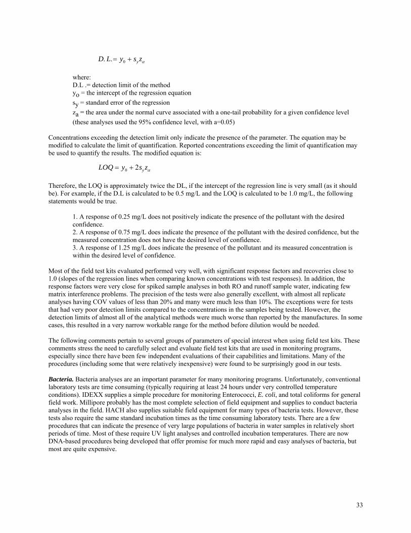
33

D L y s zy. .= +0 α

where: D.L .= detection limit of the method yo = the intercept of the regression equation sy = standard error of the regression za = the area under the normal curve associated with a one-tail probability for a given confidence level (these analyses used the 95% confidence level, with a=0.05)

Concentrations exceeding the detection limit only indicate the presence of the parameter. The equation may be modified to calculate the limit of quantification. Reported concentrations exceeding the limit of quantification may be used to quantify the results. The modified equation is:

LOQ y s zy= +0 2 α

Therefore, the LOQ is approximately twice the DL, if the intercept of the regression line is very small (as it should be). For example, if the D.L is calculated to be 0.5 mg/L and the LOQ is calculated to be 1.0 mg/L, the following statements would be true.

1. A response of 0.25 mg/L does not positively indicate the presence of the pollutant with the desired confidence. 2. A response of 0.75 mg/L does indicate the presence of the pollutant with the desired confidence, but the measured concentration does not have the desired level of confidence. 3. A response of 1.25 mg/L does indicate the presence of the pollutant and its measured concentration is within the desired level of confidence.

Most of the field test kits evaluated performed very well, with significant response factors and recoveries close to 1.0 (slopes of the regression lines when comparing known concentrations with test responses). In addition, the response factors were very close for spiked sample analyses in both RO and runoff sample water, indicating few matrix interference problems. The precision of the tests were also generally excellent, with almost all replicate analyses having COV values of less than 20% and many were much less than 10%. The exceptions were for tests that had very poor detection limits compared to the concentrations in the samples being tested. However, the detection limits of almost all of the analytical methods were much worse than reported by the manufactures. In some cases, this resulted in a very narrow workable range for the method before dilution would be needed. The following comments pertain to several groups of parameters of special interest when using field test kits. These comments stress the need to carefully select and evaluate field test kits that are used in monitoring programs, especially since there have been few independent evaluations of their capabilities and limitations. Many of the procedures (including some that were relatively inexpensive) were found to be surprisingly good in our tests. Bacteria. Bacteria analyses are an important parameter for many monitoring programs. Unfortunately, conventional laboratory tests are time consuming (typically requiring at least 24 hours under very controlled temperature conditions). IDEXX supplies a simple procedure for monitoring Enterococci, E. coli, and total coliforms for general field work. Millipore probably has the most complete selection of field equipment and supplies to conduct bacteria analyses in the field. HACH also supplies suitable field equipment for many types of bacteria tests. However, these tests also require the same standard incubation times as the time consuming laboratory tests. There are a few procedures that can indicate the presence of very large populations of bacteria in water samples in relatively short periods of time. Most of these require UV light analyses and controlled incubation temperatures. There are now DNA-based procedures being developed that offer promise for much more rapid and easy analyses of bacteria, but most are quite expensive.

34

In all cases, the user must be aware of the inherent problems in interpreting bacteria data, especially if one is using bacteria as an indicator of sewage contamination. As an example, fecal coliform bacteria are in very high populations is many waters, including stormwater that is not contaminated by sanitary sewage. The use of the fecal strep. to fecal coliform ratio to indicate sources of contamination is also inherently inaccurate, unless the source of contamination is very recent. O’Shea and Field (1992) reviewed many of these issues for stormwater. A better indication of potential sanitary sewage contamination in surface waters is the use of a small battery of chemical tracer analyses (detergents, fluoride, ammonia, and potassium), as developed and tested by Lalor (1993), Pitt, et al. (1994), and further tested by CWP and Pitt (2004). Heavy Metals. Heavy metals are also of great interest in storm studies as they are possibly the most important toxic pollutants present. However, most of the metals in stormwater are associated with particulates (Pitt, et al. 1995), with the exception of zinc, while all of the field test kits examined are only sensitive to “soluble” forms of the metals. The HACH Bicinchonate Copper Method using AccuVac Ampoules is the most suitable field method available (at a reasonable price) for measuring copper that was evaluated. This test uses the HACH DR/2000 spectrophotometer (at $1495) (or a less expensive dedicated filter spectrophotometer, at $400) and the unit test cost is $0.56. It uses AccuVac ampoules that are very easy to use and makes the test very repeatable. However, the glass ampoules do produce glass wastes. This method only indicates the presence of ionized copper. Any metallic or chelated copper will not be detected. The HACH LeadTrak system is by far the most sensitive low-cost lead field test kit available. It is capable of detecting lead concentrations as low as 1 µg/L. Unfortunately, it is also quite complex and requires extensive experience. The test also takes about 45 minutes to conduct, which may be reduced to about 15 minutes with experience and if conducting several analyses at one time. The initial test kit costs about $400 (including a dedicated filter spectrophotometer) and the per-sample cost is about $5. The LeadTrak system determines lead concentrations through colorimetric determination of a lead complex extracted from the sample. The test procedure is quite complicated, requires a large amount of space compared to the other tests, and uses hazardous chemicals. However, it does produce good results. The La Motte Zinc test was the only acceptable zinc method investigated. This test uses a dilute solution containing cyanide, whereas the alternative tests use full strength granular cyanide. The test costs about $0.60 each and requires about 5 minutes. Two very sensitive electro-chemical heavy metal field methods were also examined. The Palintest SA-1000 Scanning Analyzer is an anodic stripping voltammeter that uses pre-prepared electrode cards that come pre-calibrated. The instrument costs $2,000 (available from AZUR Environmental) and each analysis for copper and lead costs about $5.50. The test is extremely sensitive (lead to about 5 µg/L and copper to about 75 µg/L) and relatively rapid (3 minutes). Another field method evaluated is the Metalyzer 3000 from Environmental Technologies Group, Inc. This is a potentiometric voltammeter that is also capable of very sensitive simultaneous analyses of copper and lead. This instrument (which includes a built-in data logger) costs about $4,200 and each analysis for copper and lead costs about $15. Since both of these instruments do not detect particulate-bound heavy metals, their best use may be in evaluating rain water, most groundwaters, and finished drinking water, where particulate metal forms are not significant. Most surface waters and waste waters have large fractions of the metals bound to particulates and any metal analysis procedure that does not include sample digestion will likely severely under-report the total metal content. However, if one is only interested in “dissolved” metal conditions, these procedures may be quite suitable. Solids. Analyses of the amount of solids in water samples in the field is another highly desired objective. Unfortunately, that is not practical. However, dissolved solids can be estimated using a simple conductivity meter, while suspended solids may be qualitatively estimated using a field nephelometer. Secchi disk transparency has also been historically used as an indication of suspended solids (especially related to algal activity). An excellent field nephelometer is available from HACH (for $800), while turbidity “probes” (miniaturized nephelometers) are now available on several in-situ continuously recording multi- water quality probes (the Horiba HU-10 for $2,800 and the

35

YSI 6000 series, for about $7,000). Numerous pocket conductivity meters are available that have “TDS” scales. These should be avoided in lieu of standard conductivity meters, as site specific correlations between conductivity and TDS are usually required. The Horiba Twin is a very small conductivity meter that has done very well in evaluation tests. It costs about $250, but the sensor should be replaced every 6 months at a cost of $60. This meter automatically compensates for temperature effects and is suited for very small sample volumes (3-4 drops). The meter includes a standard calibration solution. The procedure is to calibrate the meter using the provided standard solution and to select the conductivity mode. The user may partially immerse the probe in the sample, or cover the probe with a few drops of sample. Another module describes the recommended procedures for monitoring particle size distributions, of great interest in stormwater monitoring studies. pH. pH is usually considered an easy parameter to measure in the field. Unfortunately, the use of most “pocket” pH meters results in very inaccurate results, as the inexpensive probes included with these meters are not very reliable or robust, especially with storage. Recently available “dry” pH probes offer better field pH measurements. However, the most common FET transistor-based probes are delicate and can be irrecoverably damaged with abrasives, or through contamination with oils and detergents. The Sentron field pH meter (at $600) is very sturdy, stores dry, and can be easily cleaned with a brush. Although the Horiba Twin pH meter is more liable to breakage with a thin glass cover, it has worked well and is much less expensive (about $300). Dissolved Oxygen. DO is a parameter that is most commonly determined in the field. The YSI line of instruments is probably the best known and most commonly used DO meters. The rapid-pulsed current DO probes from YSI are much superior to the older Clark membranes, especially if long-term monitoring is needed (such as with the in-situ continuously recording probes). Many companies supply DO probes that work well, but with varying degrees of problems associated with storage, membrane replacement, and calibration. Winkler titration is not commonly used in the field, but HACH’s digital field titrator even makes that feasible. The titration procedures work best with BOD analyses, including field titrations of BOD bottles used for in-situ photosynthesis/respiration tests. Detergents. The CHEMetrics Detergents (Anionic Surfactants) test kit was the only practical test for detergents investigated. The tests cost about $2.38 each and requires about 10 minutes. The test uses a chloroform extraction, but the test is very well designed to minimize exposure to the operator and it uses a very small amount of chemical. The CHEMetrics procedure uses a visual comparator to determine the concentration of the detergents in the sample. A small volume of sample (5 mL) is required. The method is very quick and easy. However, the method uses chloroform, a known carcinogen. Users must conduct the test in well ventilated areas. Furthermore, the waste must be disposed properly. The kit is well-designed to minimize the use and exposure of the chloroform. The reagent packs do have a limited shelf life, however. Fluoride. The HACH Fluoride SPADNS Reagent test using AccuVac Ampoules is another AccuVac test that shares the DR/2000. The tests cost about $1.17 each and requires about 5 minutes. The test does produce a small amount of glass waste and the SPADNS reagent is hazardous, requiring special disposal considerations. Two ion selective electrode (ISE) probes were also evaluated for fluoride analyses, with disappointing results. Probe problems were mostly associated with stability of the probe, especially with storage, and time consuming standardization. Similar problems were found with ISE probes for ammonia, detergents, and potassium. ISE probes may work well in controlled laboratory settings, especially with proper care of the probes, but their use in the field is probably restricted to trained electro-chemists who know how to take proper care of the probes and who know how to more efficiently calibrate them. Exceptions were the Horiba Cardy ISE probes for potassium and nitrates that have worked very well in the field, although they are not very sensitive. Nutrients. The most common nutrient tests are for ammonia nitrogen, nitrate nitrogen and phosphorus. HACH Nitrate, MR. This test also shares the DR/2000 spectrophotometer and uses AccuVacs. The test is therefore very simple and quick, but produces glass debris and a hazardous reagent waste. The test costs about $0.56 per test and takes about 7 minutes.

36

The HACH, Ammonia method using salicylate without distillation is a colorimetric determination of ammonia using salicylate. This method requires a DR/2000 spectrophotometer at $1495 (usable for several other parameters) and a per sample cost of $2.88. It is also available as a self-contained test kit with a colorimeter for about $400. Numerous simple field test kits are available for phosphorus. HACH, for example, has 8 separate spectrographic tests and 11 colorimetric tests available for different forms and concentration ranges for phosphorus. Reactive phosphorus (orthophosphate) is probably of greatest interest for most simple environmental monitoring activities. The HACH AccuVac ascorbic acid method with the DR/2000 spectrophotometer is probably the simplest test procedure available. The tests cost about $0.56 each, after purchase of the spectrophotometer. Selection of Appropriate Field Test Kits The most appropriate field test kit for a specific use can be selected based on the criteria presented earlier in this section. In most cases, the limits of detection are the most critical criterion. It is quite possible that the simplest field test kits may be useful for some studies, as most were found to be generally free from interferences (Day 1996). However, during tests using actual stormwater samples and spiked waters, their sensitivity was found to be generally poor, even less sensitive than typically advertised. This will likely lead to false negatives if actual limits of detection are not determined through sensitivity tests using local waters. The needed limits of detection must be known before analytical methods are selected, using methods presented earlier. The following example illustrates how this information can be used to select the most appropriate field testing methods, or to rely on conventional laboratory analyses. Table 7 lists the water quality parameters of most interest for stormwater monitoring, and their associated assumed variation, and corresponding needed limits of detection.

37

Table 7. Water Quality Measurements of Interest and Expected Analytical Requirements for Hypothetical Receiving Water Investigation Assessing Aquatic Life Use Impairments (Burton and Pitt 2002) Water Quality Parameter

Example Water Quality Objectives Associated with Aquatic Life Beneficial Uses (short-term exposures)

Expected Coefficient of Variation (COV) Category1

Estimated Needed MDL1

Suitable Field Measurement Methods Providing Estimated Needed MDL

Zinc <120 µg/L (CMC2) Medium 28 µg/L No available field method could approach this desired MDL. The lowest MDL found was about 140 µg/L for Zn. Most of the field test methods also require toxic (cyanide) reagents.

Copper <13 µg/L (CMC) Medium 3 µg/L No available field method could approach this desired MDL. The lowest MDL found was about 100 µg/L for Cu.

Lead <65 µg/L (CMC) Medium 15 µg/L The HACH LeadTrak system has a MDL of about 5 µg/L, although it is a time consuming test and relatively expensive. The Metalyzer 3000 and Palintest SA-1000 both have lead MDLs of about 5 µg/L and would therefore be suitable, but are expensive instruments.

Microtox screening test

n/a: indicative of toxicants that may be present (such as pesticides), desire low value; I20 of <25%.

Medium I20 of 6% Deltatox (expensive instrument, but field portable).

Hardness Narrative (want moderate to hard water conditions to reduce effect of some toxicants), would like to detect hardness to at least 50 mg/L.

Low 40 mg/L HACH Digital Titrator and CHEMetrics EDTA titration methods would both likely be suitable field methods.

Alkalinity n/a (would like moderate to high levels of alkalinity to reduce effects of some toxicants), would like to detect alkalinity to at least 25 mg/L.

Low 20 mg/L Field titration methods available, but not evaluated.

Ammonia <3.8 mg/L (2.5 X chronic at 30oC) Low 3 mg/L All 4 field test kits investigated have limits of detection better than this estimated needed MDL. However, one requires refrigeration, and others contain mercury in waste.

Nitrates n/a (rarely toxic to aquatic life in natural streams, but indicative of potential eutrophicaiton problems in nitrogen limited streams), would like to detect NO3 to at least 1 mg/L.

Low 0.8 mg/L The La Motte and CHEMetrics nitrate tests, and likely the HACH low range nitrate test, can meet this MDL objective. Sharps and cadmium containing wastes are common with these methods.

Phosphates Narrative, <25 µg/L to prevent eutrophication.

Low 20 µg/L Numerous phosphate field test kits are available, although not reviewed by Day (1996). It is expected that there are several that can meet these performance objectives.

Suspended solids

Narrative: <100 mg/L settleable fraction to prevent of smothering of streambed.

Large 12 mg/L No field instruments known for measuring suspended solids (requires drying ovens and analytical balance), but can predicted/tracked using turbidity.

COD n/a (indication of organic matter), would like to be <5 mg/L.

Medium 1 mg/L No field instruments known for measuring COD (requires digestion).

pH Between 6.5 and 9 desired (harmless to fish in this range).

Very low Readable to 0.3 pH units

All of the pH electrode methods investigated should meet this readability objective, but the pH paper methods are not likely suitable.3

Conductivity n/a (variation should be minimal), would like to determine conductivity at 100 µS/cm.

Low 80 µS/cm All three conductivity probes investigated had limits of detection about equal to this objective and would be suitable.3

Turbidity Narrative: <50 NTU increase above background conditions.

Large 6 NTU The HACH portable nephelometer, or the Horiba HU-10 and YSI in-situ probes can measure turbidity in the field, although these are all moderate to very expensive options.3

DO >5.0 mg/L Low Readable to 0.25 mg/L

Most modern field DO meters could be used to meet these objectives.3

Temperature Narrative (variation from natural conditions should be minimal).

Low Readable to 0.5 oC

Most modern field DO meters also have temperature readouts and would be suitable, alternatively, simple pocket thermometers could be used.3

1 if the COV is low (<0.5), the multiplier for the MDL is 0.8 X the desired median value of the observations, in this case taken to be the water quality objectives. If the COV is medium (0.5 to 1.25), the multiplier is 0.23, and if the COV is large (>1.25), the multiplier is 0.12. 2 CMC: criterion maximum concentration (exposure period of 1 hr) 3 The combination probes (such as the YSI 6000) should be considered as they can monitor several needed constituents: pH, conductivity, turbidity, DO, and temperature)

38

The only other primary water quality constituents noted by Burton and Pitt (2002) of great interest for receiving water assessments include microorganisms. These are currently not possible to analyze in the field, although portable sample preparation and field incubators are available from HACH and others. Because of the long sample incubation periods required (typically 18 to 24 hours for preliminary results), these methods are not really considered field methods here. Therefore, the analyses that may be possible to conduct using field test kits that meet basic sensitivity requirements include: Conventional Constituents: • hardness (using field titration equipment) • alkalinity (using field titration equipment) • turbidity (possible using moderately expensive field nephelometer, or expensive in-situ recording probes) • pH (easily conducted using electrodes, or expensive in-situ recording probes) • conductivity (easily conducted using electrodes, or expensive in-situ recording probes) • DO (easily conducted using electrodes, or expensive in-situ recording probes) • temperature (easily conducted using electrodes, thermometers, or expensive in-situ recording probes) Nutrients: • ammonia (several simple field test kits available) • nitrates (several simple field test kits available) • phosphates (several simple field test kits available) Toxicants: • lead (but difficult, time consuming, or expensive) • toxicity screening (expensive instrument) Of these, DO (field probe preferred to titration in most cases), temperature (mandatory), and pH (within a few hours) may need to be conducted in the field to meet QA/QC requirements, while conductivity is very easy to measure in the field (and therefore commonly done). The decision to measure the other constituents listed above in the field should be based on other considerations, mainly safety, cost, time, and difficulty. In many cases, it is not practical to conduct field measurements at the time of sample collection due to the time needed to setup equipment, standardize the procedures, and conduct the individual constituent analyses at each sampling location. However, it may be very reasonable to use these field methods in a temporary field laboratory when conducting sampling in remote areas. In this case, samples collected over a short period of time (such as during the day) can be analyzed together, minimizing the time requirements. In addition, the use of continuous recording in-situ probes should be seriously considered for turbidity, conductivity, pH, DO, and temperature, in addition to possibly ORP and stream stage (depth). Although expensive (can be rented for short periods), these probes have been extremely useful when monitoring these key constituents over several week periods of time that include both wet and dry periods. The high resolution data (measurements typically are taken and logged every 15 minutes) dramatically illustrates the variabilities of these constituents over short periods of time (as discussed in the narratives for some of the water quality criteria) and helps to understand the duration of exposure to wet weather related discharges. Conventional Laboratory Analyses Table 8 lists standard analytical methods that may be used for stormwater analyses. Several methods need to be modified to effectively analyze stormwater samples, especially if small sample volumes are only available (such as from porewater from stream sediments, from bench-scale treatability tests, or to reduce sample shipping costs). Modifications to the standard methods are described by Burton and Pitt (2002) and were necessitated because of the large particulate fractions of the organic toxicants which interfered with conventional extraction methods. Reducing the sample volumes (especially for the organic analyses) also significantly reduces the volumes of hazardous laboratory wastes generated. This table should not be considered as a complete listing of laboratory methods for stormwater analyses, but is an example of some analyses and the associated standard methods. Burton and Pitt (2002) contains descriptions of the modifications to the standard methods for the organic toxicants noted in the above table that are needed for effective measurements of stormwater characteristics. These

39

modifications are needed to obtain necessary levels of recovery of the organics that are bound to particulates in the stormwater. These methods rely on continuous extraction methods (separation funnels and multiple extracting solutions). More convenient solid phase extraction (SPE) methods have been shown to have very poor (sometimes negative) recoveries with stormwater samples. Under a current NSF-sponsored project, we are evaluating thermal-desoprtion extraction methods for organics bound to particulates. This method is showing great promise by allowing stormwater particulates to be captured on various filters for direct analysis and the filtrates can then be analyzed by SPE (but require SIM analytical methods for added sensitivity). Table 8. Typical List of Standard and Modified Methods for Wet Weather Flow Analyses

Parameter Method

PHYSICAL ANALYSES

Color, Spectrophotometric EPA 110.3 Conductance, Specific Conductance EPA 120.1 Particle size analysis by Coulter Counter and sieves Coulter method pH, Electrometric EPA 150.1 Residue, filterable, gravimetric, dried at 180 oC EPA 160.1 Residue, non-filterable, gravimetric, dried at 103-105 oC EPA 160.2 Residue, total, gravimetric, dried at 103-105 oC EPA 160.3 Residue, volatile, gravimetric, ignition at 550 oC EPA 160.4 Turbidity, nephelometric EPA 180.1

INORGANIC ANALYSES

Hardness, Total (mg/L as CaCO3), Titrimetric EDTA EPA 130.2 Aluminum, arsenic, cadmium, chromium, copper, iron, lead, nickel, and zinc EPA 200.9 Chloride, fluoride, nitrate, nitrite, phosphate, and sulfate EPA 300.0 Ammonium, calcium, lithium, magnesium, potassium, and sodium EPA 300.0

modified Alkalinity, titrimetric (pH 4.5) EPA 310.1

ORGANIC ANALYSES

Chemical Oxygen Demand, colorimetric EPA 410.4 Aldrin, Chlordane-alpha, Chlordane-gamma, 4,4'-DDD, 4,4'-DDE, 4,4'-DDT, Dieldrin, Endosulfan I, Endosulfan II, Endosulfan sulfate, Endrin, Endrin aldehyde, Endrin ketone, HCH-alpha, HCH-beta, HCH-gamma (Lindane), Heptachlor, Heptachlor epoxide, and Methoxychlor

EPA 608 modified

Acenaphthene, Acenaphthylene, Anthracene, Azobenzene, Benzo(a)anthracene, Benzo(b)fluoranthene, Benzo(g,h,i)perylene, Benzo(k)fluoranthene, Benzo(a)pyrene, 4-Bromophenyl-phenylether, Bis-(2-chloroethyl)ether, Bis-(2-chloroethoxy)methane, Bis-(2-ethylhexyl)phthalate, Butylbenzyl phthalate, Carbazole, 4-Chloro-3-methylphenol, 2-Chloronaphthalene, 2-Chlorophenol, 4-Chlorophenyl-phenylether, Chrysene, Coprostanol, Dibenzo(a,h)anthracene, 1,2-Dichlorobenzene, 1,3-Dichlorobenzene, 1,4-Dichlorobenzene, 2,4-Dichlorophenol, Diethyl phthalate, 2,4-Dimethylphenol, Dimethyl phthalate, Di-n-butyl phthalate, 2,4-Dinitrophenol, 2,4-Dinitrotoluene, 2,6-Dinitrotoluene, Di-n-octyl phthalate, Fluoranthene, Fluorene, Hexachlorobenzene, Hexachlorobutadiene, Hexachlorocyclopentadiene, Hexachloroethane, Indeno(1,2,3-cd)pyrene, Isophorone, 2-Methylnaphthalene, 2-Methylphenol, 4-Methylphenol, Naphthalene, Nitrobenzene, 2-Nitrophenol, 4-Nitrophenol, N-Nitroso-di-n-propylamine, N-Nitroso-diphenylamine, Pentachlorophenol, Phenanthrene, Phenol, Pyrene, 1,2,4-Trichlorobenzene, 2,4,Trichlorophenol, and 2,4,6-Trichlorophenol

EPA 625 modified

Toxicity Analyses

Microtox™ 100% toxicity screening analysis (using reagent salt for osmotic adjustments) Azur Environmenal method

Burton and Pitt (2002)

40

Quality control and quality assurance activities require a substantial effort in most analytical laboratories. EPA analytical guidelines published in the Federal Register for the different tests specify the types and magnitude of QA/QC analyses. These analyses supplement the standardization efforts as they are used to measure the efficiency of the sample preparation and analysis procedures. Blanks are used to identify possible contamination problems, while matrix spikes added to the samples prior to any preparation steps indicate the efficiency of the complete analytical process. Spikes added to the samples prior to analyses are also used to identify interferences, mainly associated with other compounds in the sample. In heavy metal analyses, for example, it is not uncommon to increase the sample analysis effort by an extra 50% for standards and QA/QC samples in production work. Method development activities would require even a greater additional analytical effort. Reporting Results Affected by Detection Limits Reporting chemical analysis results should be clear, based on the measured detection limits and QA/QC program. Concentrations below the IDL are not present with sufficient confidence to detect them as significantly different from the baseline random noise of the instrument. These should be reported as not detected (generally given a “U” qualifier in organic compound analytical reports). Concentrations of a parameter above the IDL, but below the MDL are present, but the confidence in the concentration value is less than 99% (can be given a “J” qualifier in organic analytical reports). Concentrations above the MDL indicate that the parameter is present in the sample and that the reported concentration is certain, at the 99% confidence level, or greater. Many other conditions may be present that degrade the confidence of the analytical results. These should all be carefully noted in the analytical report. As noted in the module on statistical analysis methods, non-detected (“left-censored”) values present special problems in analyzing data. If only a few (or most) of the observations are below the detection limit, these problems are not very serious. However, if the detection limit available results in many left-censored data (say between 25 and 75% of the observations), statistical analyses are severely limited. It may not be possible to completely statistically evaluate the effectiveness of a treatment process, for example, if many of the effluent concentrations of a critical pollutant are below the detection limit, even if the influent concentrations are well above the MDL. The removal of the pollutant is obviously important and effective, but it is not possible to calculate the significance of the differences in the observed concentrations. From a statistical (and engineering) viewpoint, it would be better if all concentrations determined by the analytical procedure be reported, even if they are below the designated “formal” detection limit, set using an extreme 99% confidence limit. The use of the qualifiers (such as U and J as used in reporting GC/MS data) along with the numeric values and obvious reporting of the MDL should serve as a warning for the limited use of these values. However, analytical chemists are justifiably concerned about the misuse of “non-detected” values and the availability of these values for statistical analyses will likely remain elusive. The percentage of censored observations in a dataset affects the calculated mean, median, standard deviation and coefficient of variation values. As the level of non-detected observations increase, the mean, median and standard deviation are larger than if the censored observations are detected. The opposite behavior is expected for the coefficient of variation. Different laboratories report different detection limits for the same constituents. In many cases, the detection limits are calculated by each laboratory based on their measured repeatability (precision) for a specific laboratory test. Using methods with low precision increases the percentage of non-detected values and the uncertainty of the real mean and standard deviation values. During the NSQD database development, Maestre and Pitt (2005) found that open space sampling sites had the largest number of non-detected observations among all of the land uses monitored. The largest percentages of detected observations were observed in freeways and industrial land uses. Statistical tests conducted to determine the effects of varying amounts of undetected values, and the usual substitution methods, were therefore conducted. Estimating or replacing by half of the detection limit for levels of censoring smaller than 5% does not have a significant effect on the mean, standard deviation and coefficient of variation values. However, replacing the censored observations by half of the detection limit is not recommended for levels of censoring larger than 15%. The censored observations in the database were replaced using estimated values using Cohen’s maximum likelihood method for each site before the statistical tests. Because this method uses the detected observations to estimate the non-detected values (based on the probability distribution of the available data), it is not very accurate, and therefore not recommended, when the percentage of censored observations is larger than 40%.

41

The different methods for handling censored data all present different types of problems when analyzing the data. These problems would not occur if suitable detection limits were used. It is therefore very important to select analytical methods capable of detecting the desired range of concentrations in the samples in order to reduce the numbers of censored observations to acceptable levels. Table 9 summarizes the recommended minimum detection limits for various stormwater constituents to obtain manageable non-detection frequencies (<5%). Some of the open space stormwater measurements (oil and grease and lead, for example), would likely have greater than 5% non-detects, even with the detection limits shown. The detection limits for filtered heavy metals would be substantially less than shown on this table. Table 9. Suggested Analytical Detection Limits for Stormwater Monitoring Programs to Obtain <5% Non-detects Residential, commercial,

industrial, freeway Open Space

Conductivity 20 µS/cm 20 µS/cm Hardness 10 mg/L 10 mg/L Oil and grease 0.5 mg/L 0.5 mg/L TDS 10 mg/L 10 mg/L TSS 5 mg/L 1 mg/L BOD5 2 mg/L 1 mg/L COD 10 mg/L 5 mg/L Ammonia 0.05 mg/L 0.01 mg/L NO2+NO3 0.1 mg/L 0.05 mg/L TKN 0.2 mg/L 0.2 mg/L Dissolved P 0.02 mg/L 0.01 mg/L Total P 0.05 mg/L 0.02 mg/L Total Cu 2 µg/L 2 µg/L Total Pb 3 µg/L (residential 1 µg/L) 1 µg/L Total Ni 2 µg/L 1 µg/L Total Zn 20 µg/L (residential 10 µg/L) 5 µg/L Maestre and Pitt (2005) References ASTM (American Society of Testing and Materials). 1996 Annual Book of ASTM Standards. West Conshohocken,

PA: ASTM, vol. 04.08, 1994. Behera, Pradeep K., James Y. Li, and Barry J. Adams. “Characterization of Urban Runoff Quality: A Toronto Case

Study”. In: Applied Modeling of Urban Water Systems. Guelph, Ontario: Computational Hydraulics International: (James W. Ed.) CHI. 2000.

Burton, G.A. Jr., and R. Pitt. Stormwater Effects Handbook: A Tool Box for Watershed Managers, Scientists, and Engineers. ISBN 0-87371-924-7. CRC Press, Inc., Boca Raton, FL. 2002. 911 pages.

Center for Watershed Protection and R. Pitt. Illicit Discharge Detection and Elimination; A Guidance Manual for Program Development and Technical Assessments. U.S. Environmental Protection Agency, Office of Water and Wastewater. EPA Cooperative Agreement X-82907801-0. Washington, D.C., 357 pgs. Oct. 2004.

Day, J. Selection of Appropriate Analytical Procedures for Volunteer Field Monitoring of Water Quality. MSCE thesis, Dept. of Civil and Environmental Engineering, University of Alabama at Birmingham. 1996.

EPA (U.S. Environmental Protection Agency). Results of the Nationwide Urban Runoff Program. Water Planning Division, PB 84-185552, Washington, D.C., December 1983.

Gibbons, Jean, and Subhabrata Chakraborti. Nonparametric Statistical Inference. New York, NY: Marcel Dekker Inc. 2003.

Kottegoda, Nathabandu T., and Renzo Rosso. Statistics, Probability and Reliability for Civil and Environmental Engineers. New York, NY: WCB McGraw-Hill. 1998.

Lalor, M. An Assessment of Non-Stormwater Discharges to Storm Drainage Systems in Residential and Commercial Land Use Areas. Ph.D. Dissertation. Department of Civil and Environmental Engineering. Vanderbilt University. 1994.

42

Maestre, A. and R. Pitt. The National Stormwater Quality Database, Version 1.1, A Compilation and Analysis of NPDES Stormwater Monitoring Information. U.S. EPA, Office of Water, Washington, D.C. (final draft report) August 2005.

Massey, Frank J. Jr. “A Note on the Power of a Nonparametric Test”. Annals of Mathematical Statistics 21 : 440 – 43. 1950.

Massey, Frank J. Jr. “The Kolmogorov-Smirnov Test for Goodness of Fit”. Journal of the American Statistical Association 46 : 67 – 78. 1951.

McCormick, D, and A. Roach. Measurement, Statistics and Computation. John Wiley & Sons. Chicester, UK. 1987 O’Shae, M. and R. Field. “An evaluation of bacterial standards and disinfection practices used for the assessment

and treatment of stormwater. Advances in Applied Microbiology. Acad. Press, Inc. Vol. 37, no. 21-36. 1992a. O’Shae, M. and R. Field. “Detection and disinfection of pathogens in storm-generated flows.” Canadian Journal of

Microbiology. Vol. 48, no. 4, pp. 267-276. April 1992b. Pitt, R. and G. Shawley. A Demonstration of Non-Point Source Pollution Management on Castro Valley Creek.

Alameda County Flood Control and Water Conservation District and the U.S. Environmental Protection Agency, Water Planning Division (Nationwide Urban Runoff Program). Washington, D.C. June 1982.

Pitt, R., S. Clark, and K. Parmer. Protection of Groundwater from Intentional and Nonintentional Stormwater Infiltration. U.S. Environmental Protection Agency, EPA/600/SR-94/051. PB94-165354AS, Storm and Combined Sewer Program, Cincinnati, Ohio. 187 pgs. May 1994.

Pitt, Robert, and John Voorhees. Source Loading and Management Model (SLAMM). In: Seminar Watershed Management at the local, County, and State Levels. Center for Environmental Research Information. United States Environmental Protection Agency EPA: EPA/625/R-95/003. Cincinnati, Ohio. 1995.

Pitt, R., R. Field, M. Lalor, and M. Brown. “Urban stormwater toxic pollutants: assessment, sources and treatability.” Water Environment Research. Vol. 67, No. 3, pp. 260-275. May/June 1995.

Pitt, R. and Lalor, M. Assessment Strategy for Evaluating the Environmental and Health Effects of Sanitary Sewer Overflows from Separate Sewer Systems. First Year Report. Wet-Weather Flow Management Program, National Risk Management Research Laboratory, U.S. Environmental Protection Agency, Cincinnati, Ohio. January 1998.

Pitt, R. and U. Khambhammettu. Field Verification Tests of the UpFlowTM Filter. Small Business Innovative Research, Phase 2 (SBIR2) Report. U.S. Environmental Protection Agency, Edison, NJ. 275 pages. March 2006.

Standard Methods for the Examination of Water and Wastewater. 19th edition. Water Environment Federation. Washington, D.C. 1995.

Van Buren, Mark, Edgar Watt, and Jiri Marsalek. “Application of the Lognormal and Normal Distribution to Stormwater Quality Parameters”. Water Research 31 (1): 95 – 104. 1997.