Fakultät für Physik und Geowissenschaften

Physikalisches Grundpraktikum

1

M8e “Fourier Analysis of Acoustic Oscillations” Tasks

In order to familiarize yourself with the experimental setup and the potential of Fourier analysis,

analyze various acoustic phenomena (e.g. tone, sound, noise, your own musical instrument) using

Fast-Fourier Transformation (FFT).

1. Measure the dependence of the eigenfrequency of a tuning fork on the position of an additional

mass (detuning mass) placed on one of the prongs of the tuning fork. Further determine the

frequency spectrum of the superposition of two tuning forks, one with the original tone and the

second one detuned, using FFT. Represent the resulting beat in time and in frequency space.

2. Measure the frequency of the air column vibrations in round bottom flasks (Helmholtz resonators)

with various dimensions. Compare the experimental results to the calculated eigenfrequencies for

Helmholtz resonators.

3. Measure the eigenfrequencies of vibration on a string using a monochord with various string

lengths and tensions. Plot the eigenfrequencies in an appropriate way, determine the slopes of the

resulting straight lines and compare these to the theoretical expressions.

Literature

Physikalisches Praktikum, 14. Imprint, Editors W. Schenk, F. Kremer, Fourier-Transformation und

Signalanalyse, 1.0, 1.3, Mechanik 4.0, Wärmelehre 2.2.3

http://dx.doi.org/10.1007/978-3-658-00666-2

Ingenieurakustik: Physikalische Grundlagen und Anwendungsbeispiele, H. Henn, G. R. Sinambari, M.

Fallen, 4. Imprint, S. 308

http://dx.doi.org/10.1007/978-3-8348-9537-0

Physics, M. Alonso and E. J. Finn, 1992, Chap. 28. Wave motion

Physics, P. A. Tipler, 3rd Edition, Chaps. 13, 14

The Theory of Sound, J. W. Strutt, Baron Rayleigh, 1894

Accessories

CASSY-Interface, PC, microphone with amplifier, three tuning forks, detuning masses, striking

hammer (rubber, metal), various round bottom flasks, loudspeaker, synthesizer (software),

monochord, tension device with force sensor

2

Keywords for preparation

- Mechanical oscillations and waves, wave equation, standing waves

- Natural vibrations, resonance, fundamental frequency and overtones

- Sound wave, sound velocity, differences between tone, sound and noise

- Fourier analysis, Fourier spectra of sine, square and triangular signals

- Tuning fork vibrations, flexural vibrations, eigenfrequency of a tuning fork

- Air chamber oscillations, adiabatic state transformations, eigenfrequency of a Helmholtz resonator

- Vibrations on a string, wave equation for a string, fundamental frequency and overtones of strings

- Experimental setup for the excitation, measurement and evaluation of various sound waves

- Fundamentals of digital measurements (sampling rate, resolution)

General principles

Vibrations on a tuning fork

The vibrations of the prongs of a tuning fork might be understood in analogy to flexural vibrations on a rod. This leads to transverse oscillations perpendicular to the axis of the prong at rest. These do not follow the standard wave equation, but a differential equation which is of fourth order in the position coordinate:

2 4

2 4

E I

At x

. (1)

denotes the amplitude of flexural vibrations. The eigenfrequencies fn of the flexural vibrations are found as

2

2,

2πn

n

E Imf

l A

(2)

with the area moment of inertia I of a rod with cross sectional area A, the length of the rod l,

Young’s modulus E and the mass density of the rod material. The values mn are solutions of the

transcendental equation cos cosh 1n nm m , with m1 = 1.875 for the fundamental.

The generation of as sound wave in air by the vibrations of a tuning fork can be understood by the

adiabatic expansion and compression of the air layers surrounding the prongs. The resulting pressure

changes propagate with the speed of sound cAir which for temperatures close to room temperature

T ( 0 0T T T , T0 = 273.15 K) is given in good approximation by

10Air

0

331.5 1 ms2

T Tc

T. (3)

3

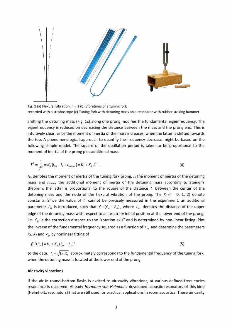
Fig. 1 (a) Flexural vibration, n = 1 (b) Vibrations of a tuning fork

recorded with a stroboscope (c) Tuning fork with detuning mass on a resonator with rubber striking hammer

Shifting the detuning mass (Fig. 1c) along one prong modifies the fundamental eigenfrequency. The

eigenfrequency is reduced on decreasing the distance between the mass and the prong end. This is

intuitively clear, since the moment of inertia of the mass increases, when the latter is shifted towards

the top. A phenomenological approach to quantify the frequency decrease might be based on the

following simple model. The square of the oscillation period is taken to be proportional to the

moment of inertia of the prong plus additional mass:

2 20 SG R Steiner 1 22

1( )T K I I I K K

f . (4)

ISG denotes the moment of inertia of the tuning fork prong, IR the moment of inertia of the detuning

mass and ISteiner the additional moment of inertia of the detuning mass according to Steiner’s

theorem; the latter is proportional to the square of the distance between the center of the

detuning mass and the node of the flexural vibration of the prong. The Ki (i = 0, 1, 2) denote

constants. Since the value of cannot be precisely measured in the experiment, an additional

parameter 0 is introduced, such that m 0( ) , where m denotes the distance of the upper

edge of the detuning mass with respect to an arbitrary initial position at the lower end of the prong;

i.e. 0 is the correction distance to the “rotation axis” and is determined by non-linear fitting. Plot

the inverse of the fundamental frequency squared as a function of m and determine the parameters

K1, K2 and 0 by nonlinear fitting of

2 21 m 1 2 m 0( ) ( )f K K . (5)

to the data. 1 1

1/f K approximately corresponds to the fundamental frequency of the tuning fork,

when the detuning mass is located at the lower end of the prong.

Air cavity vibrations

If the air in round bottom flasks is excited to air cavity vibrations, at various defined frequencies

resonance is observed. Already Hermann von Helmholtz developed acoustic resonators of this kind

(Helmholtz resonators) that are still used for practical applications in room acoustics. These air cavity

4

vibrations might be described in analogy to the oscillation of a typical mass-spring system (mass m,

spring constant k). The eigenfrequency of this system is given by

0

1

2π

kf

m . (6)

The compressible gas volume VH of the cavity, see Fig. 2, acts like a spring on the air mass m = mG

located in the flask neck (gas mass mG = G l A , l length of the resonator neck, A cross-sectional area

of the oscillating mass, G density of the gas at rest).

Fig. 2 Model of a Helmholtz resonator

First the “spring constant” k of the gas volume is calculated. Under the assumption that pressure

changes in the gas occur so fast that no heat exchange with the surroundings occur, one obtains for

the adiabatic bulk modulus K:

H G

Δ

Δ

pK V p

V . (7)

denotes the adiabatic index (heat capacity ratio) and pG the pressure of the gas at rest. The

pressure change p is induced by a force F acting on the area A:

Fp

A

. (8)

A displacement of the oscillating gas mass mG from its rest position by a distance l in the direction

of the cavity volume VH leads to a reduction of the resonator volume by V. Accordingly, volume and

length change have opposite signs: V = A l. Using Eqs. (7) and (8) the spring constant is obtained

as

2G

H

Δ

Δ

p AFk

l V

. (9)

Inserting k and mG in Eq. (6) yields

G0

H G

1

2π

Apf

V l

. (10)

An exact calculation shows that the flask neck l has to be corrected by the so-called spout correction

( / 4R , R radius of the flask neck, see Fig. 2) on both sides of the resonator neck; this yields the

eigenfrequency f0 of the Helmholtz resonator

5

2 2G

0 G

H G H

π π1 1

π π2π 2π

2 2

p R Rf c

R RV l V l

. (11)

cG in Eq. (11) is the sound velocity of the gas in the resonator volume.

Vibrations on a string

Transverse vibrations on a string are treated under the assumption that the material is elastic, has a

diameter (in case of a circular cross section) much smaller than the length and that shear effects are

negligible. Consider a string fixed at both ends and subjected to a certain tension. If the string is set

into vibration, nodes appear at the end. Besides the fundamental frequency f1 there might be

overtones at higher frequencies fn = n f1 (n > 1). Apart from the nodes at the fixed ends the n-th

overtone has (n-1) additional nodes (Fig. 3).

Fig. 3 Standing waves on a string for the fundamental and the first and second overtone; the ends are clamped.

For the derivation of the equation of motion consider the force that vertically restores a piece of

string back to its rest position. This force is supplied by the string tension τ = F / A, (force F per cross

sectional area A of the string). In case of a curved string, a force component Fy (Fig. 4) results, since

the tension acting on each mass element of the string is equal in magnitude, but not necessarily

along the same direction.

Abb. 4 String segment dm with forces Fy (curvature strongly exaggerated)

For the restoring force components Fy in the y-direction (with the x-direction oriented along the rest

position of the string) one obtains at positions x and x+dx ( ) sinyF x A and

( d ) sin( d )yF x x A , respectively. In the following it is assumed that the angles of inclination

of the string with respect to its rest position are small, such that to a good approximation sin ,

6

sin(+d) + d, cos cos( + d) 1, tan = dy/dx and 2( / ) 1dy dx . The resulting force

in the y-direction is then given by

( ) ( ) dy y ydF F x dx F x A . (12)

In the small angle limit one has

tany

x

(13)

and therefore obtains for the change in angle between x and x+dx

2

2d d d

y

x yx x

x x

. (14)

The restoring force Fy accelerates the string element with the mass

1/22 2 1/2 2d (d ) 1 ( / ) dm A x dy A dy dx dx A x (15)

towards its rest position. According to Newton’s second law one has

2

2dy

ydF A x

t

. (16)

Setting Eqs. (12) and (16) equal and introducing 2 /c one obtains the wave equation

2 22

2 2

y yc

t x

, (17)

where c denotes the phase velocity of the transversal waves. With the relationship c f

(wavelength , frequency f ) one obtains for the fundamental (f = f1)

1

1 Ff

A . (18)

On a string with length L that is clamped on both sides a standing wave might form. In the

fundamental mode nodes appear at the clamped ends and an antinode in the middle of the string,

such that L = /2. With Eq. (18) this yields a frequency

1

1

2

Ff

L A . (19)

The general solution of the wave equation (17) has the form , /y x t y t x c , where y is an

arbitrary, twice differentiable function. Consider a wave moving along the (-x)-direction. This is

reflected at the clamping point (x = 0) and acquires a phase shift of . The superposition of incoming

and reflected wave yields:

0 0

2π 2π 2π 2π 2π 2π( , ) sin sin π 2 cos sin

t x t x t xy x t y y

T T T

. (20)

7

This solution automatically satisfies the boundary condition y(x = 0) = 0; the second clamping

condition y(x = L) = 0 imposes a restriction on the possible values of the wavelength, namely

2, 1,2, 3,...n

Ln

n . (21)

n denotes the wavelengths of the standing wave modes on a string of length L that is clamped at

both ends. This yields for the frequencies of the higher harmonics

2n

n Ff

L A . (22)

Experimental procedures

A microphone with integrated amplifier is used to measure the various sound signals; the amplifier is

connected to a CASSY-Interface system for AD-conversion and transmission of the digitized signals to

a PC. This system enables signal recording and Fourier transformation by the integrated Fast-Fourier

Transform (FFT) algorithm. Note additional instructions for the use of the microphone as well as for

the data processing in the laboratory.

Fig. 5 Experimental setup: (a) sound sources (I tuning fork, II air cavity resonator, III monochord), (b) microphone, (c) loud speaker

At the beginning of the experiment various sound waves (e.g. sine tone and "white noise", both

generated with a synthesizer, your own voice) should be measured and analyzed using the frequency

spectrum obtained from a FFT. The measurement settings (sampling rate, see Nyquist-Shannon

theorem, and signal intensity) have to be optimized in order to achieve an error-free sound

recording.

Task 1: For the realization of the measurements three identical tuning forks are available that might

be detuned by positioning a small additional mass onto one of the prongs, see Fog. 1c. To optimize

the signal amplitude the microphone is positioned close to the opening of the wooden resonator and

the amplifier gain is adjusted accordingly. Use a rubber striking hammer to generate the sound. Some

of the tuning forks have positioning marks on the prongs such that the detuning mass might be

8

clamped at well-defined positions. Measure the fundamental frequency 1f for about eight positions

m of the detuning mass. Plot 21f versus m and determine the parameters in Eq. (5) by nonlinear

fitting. Discuss the values of the parameters K1 and 0 . Further, detune one of the tuning forks and

measure the beat signal resulting from the superposition of the sound from an original and a

detuned tuning fork. Represent the signal both as a function of time and frequency. Determine the

beat period from both plots and compare the two values.

Fig. 6 Example of a signal f (t) resulting from the superposition of three tuning fork vibrations with the frequencies f1, f2, f3 as well as its Fourier transform.

Task 2: The microphone is positioned just above the top of the flask neck, see Fig. 7.

Fig. 7 Experimental setup for the frequency measurement of the air cavity resonator: round bottom flask with neck (a), microphone (b), loudspeaker (c).

Generate "white noise" with a synthesizer program; the loudspeaker is positioned close to the flask such that its sound field excites vibrations in the cavity. Record the sound in the flask neck during the excitation and generate a frequency spectrum using FFT. Determine the fundamental frequency. Alternatively, the air cavity vibrations might be excited by striking the flask with a rubber hammer. Calculate the fundamental frequencies of the various flasks, see table 1 for the respective dimensions, and compare with the experimentally determined values.

Nominal volume 50ml 100ml 250ml 500ml

Setup I R / mm 9,83(±0,1) 9,08(±0,1) 15,2(±0,1) 14,1(±0,1)

l / mm 38(±2) 38(±2) 39(±2) 37(±2)

VH / ml 60 130 298 535

Setup II R / mm 10,6(±0,1) 9,1(±0,1) 14,4(±0,1) 14,4(±0,1)

l / mm 36(±2) 36(±2) 38(±2) 39(±2)

VH / ml 60 130 298 535 Table 1: Dimensions of the round bottom flasks.

9

Task 3: Vibrations on a string are studied as a function of the string length and the string tension. To

this end thin metal wires are spanned to a monochord which acts as a sound amplifier. For the length

variation a movable wedge might be shifted along the length of the monochord. The tension in the

string might be varied by a tension device controlled by a force sensor.

Fig. 8 String spanned onto a monochord.

String vibrations are excited by plucking the string. The microphone is positioned directly above the

string to optimize the signal intensity. Fig. 9 shows an example of a recorded time signal and its Fast-

Fourier Transform; the fundamental frequency as well as several higher harmonics can be clearly

seen.

Fig. 9 Time signal and FFT of a string vibration with fundamental frequency f1 and higher harmonics f2 to f5

The higher harmonics might be used to unambiguously identify the fundamental frequency, since

f1 = fn / n. In case of the tension dependence, the measured fundamental frequencies should be

plotted in a 1f F -diagram, in case of the length dependence, a 11f L -diagram should be used.

Determine the slopes of the resulting straight lines and compare with the values calculated from Eq.

(19). To this end measure length L and diameter (2r) of the string; the density of steel is =

7850 kgm-3.