m8s2 - regression in practice - jarad.me · m8s2 - regression in practice professor jarad niemi...
TRANSCRIPT

M8S2 - Regression In Practice
Professor Jarad Niemi
STAT 226 - Iowa State University
December 4, 2018
Professor Jarad Niemi (STAT226@ISU) M8S2 - Regression In Practice December 4, 2018 1 / 21
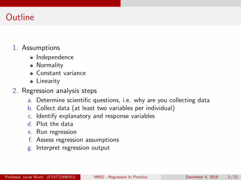
Outline
1. Assumptions
IndependenceNormalityConstant varianceLinearity
2. Regression analysis steps
a. Determine scientific questions, i.e. why are you collecting datab. Collect data (at least two variables per individual)c. Identify explanatory and response variablesd. Plot the datae. Run regressionf. Assess regression assumptionsg. Interpret regression output
Professor Jarad Niemi (STAT226@ISU) M8S2 - Regression In Practice December 4, 2018 2 / 21

Assumptions
Regression assumptions
Regression model
yi = β0 + β1xi + εi εiiid∼ N(0, σ2)
Regression assumptions are
Errors are independent
Errors are normally distributed
Errors are identically distributed with a mean of 0 and constantvariance of σ2
Linear relationship between explanatory variable and mean of theresponse
Professor Jarad Niemi (STAT226@ISU) M8S2 - Regression In Practice December 4, 2018 3 / 21

Assumptions Linearity
Assessing linearity assumption
Look for non-linearity in
response vs explanatory plot
residuals vs explanatory plot
residuals vs predicted value plot
2 4 6 8
010
2030
4050
60
explanatory
resp
onse
2 4 6 8
−5
05
explanatory
resi
dual
s
−10 0 10 20 30 40 50−
50
5
predicted
resi
dual
s
Professor Jarad Niemi (STAT226@ISU) M8S2 - Regression In Practice December 4, 2018 4 / 21

Assumptions Constant variance
Assessing constant variance assumption
Look for a trumpet horn pattern
residuals vs explanatory plot
residuals vs predicted value plot
0 2 4 6 8
−10
0−
500
50
explanatory
resp
onse
0 2 4 6 8
−50
050
explanatory
resi
dual
s
−10 −5 0 5−
500
50predicted
resi
dual
s
Professor Jarad Niemi (STAT226@ISU) M8S2 - Regression In Practice December 4, 2018 5 / 21

Assumptions Normality
Assessing normality assumption
Deviations from a straight line in a normal quantile plot (qq-plot)
2 4 6 8
−10
05
1015
explanatory
resp
onse
−2 −1 0 1 2−
10−
50
510
Normal Q−Q Plot
Theoretical Quantiles
Sam
ple
Qua
ntile
s
Professor Jarad Niemi (STAT226@ISU) M8S2 - Regression In Practice December 4, 2018 6 / 21

Assumptions Independence
Assessing the independence assumption
The main ways that the independence assumption is violated are
temporal effects
spatial effects
clustering effects
Each of these requires a relatively sophisticated plot or analysis and thus,for this course, we will assess the independence assumption using thecontext of the problem. If one of the above effects are present in theproblem, then there may be a violation of the independence assumption.
Professor Jarad Niemi (STAT226@ISU) M8S2 - Regression In Practice December 4, 2018 7 / 21

Assumptions Independence
Influential individuals
In addition to violation of model assumptions, we should be on the lookoutfor individuals who are influential.
Recall
if the explanatory variable value is far from the other explanatoryvariable values, then the individual has high leverage, and
if removing an observation changes the intercept or slope a lot, thenthe individual has high influence.
Professor Jarad Niemi (STAT226@ISU) M8S2 - Regression In Practice December 4, 2018 8 / 21
Assumptions Independence
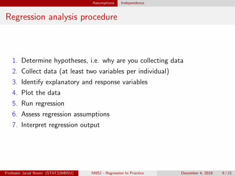
Regression analysis procedure
1. Determine hypotheses, i.e. why are you collecting data
2. Collect data (at least two variables per individual)
3. Identify explanatory and response variables
4. Plot the data
5. Run regression
6. Assess regression assumptions
7. Interpret regression output
Professor Jarad Niemi (STAT226@ISU) M8S2 - Regression In Practice December 4, 2018 9 / 21
Gas mileage
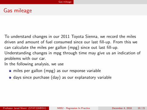
Gas mileage
To understand changes in our 2011 Toyota Sienna, we record the milesdriven and amount of fuel consumed since our last fill-up. From this wecan calculate the miles per gallon (mpg) since out last fill-up.Understanding changes in mpg through time may give us an indication ofproblems with our car.In the following analysis, we use
miles per gallon (mpg) as our response variable
days since purchase (day) as our explanatory variable
Professor Jarad Niemi (STAT226@ISU) M8S2 - Regression In Practice December 4, 2018 10 / 21
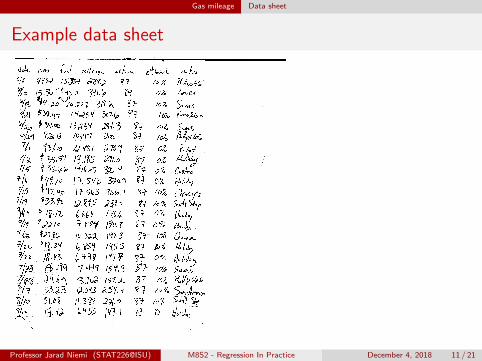
Gas mileage Data sheet
Example data sheet
Professor Jarad Niemi (STAT226@ISU) M8S2 - Regression In Practice December 4, 2018 11 / 21
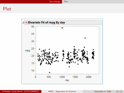
Gas mileage Plot
Plot
Professor Jarad Niemi (STAT226@ISU) M8S2 - Regression In Practice December 4, 2018 12 / 21

Gas mileage Regression output
Regression
Professor Jarad Niemi (STAT226@ISU) M8S2 - Regression In Practice December 4, 2018 13 / 21

Gas mileage Residual plots
Residuals
Professor Jarad Niemi (STAT226@ISU) M8S2 - Regression In Practice December 4, 2018 14 / 21

Gas mileage Normal quantile plot
Normal quantile plot
Professor Jarad Niemi (STAT226@ISU) M8S2 - Regression In Practice December 4, 2018 15 / 21

Gas mileage Regression output
Regression
Professor Jarad Niemi (STAT226@ISU) M8S2 - Regression In Practice December 4, 2018 16 / 21

Gas mileage Interpretation
Interpretation
When the car was purchased (day 0), the predicted miles per gallonswas 18.6 mpg.
Each additional day that passes, the miles per gallons increases by0.0008 mpg on average. Over the course of a year, this is an increaseof 0.29 mpg on average.
Only 2.9% of the variability in miles per gallon is explained by day.
Professor Jarad Niemi (STAT226@ISU) M8S2 - Regression In Practice December 4, 2018 17 / 21
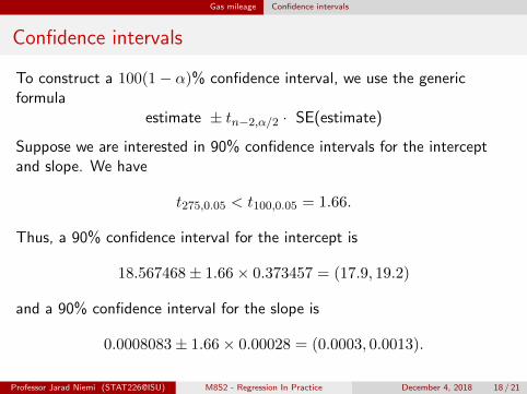
Gas mileage Confidence intervals
Confidence intervals
To construct a 100(1− α)% confidence interval, we use the genericformula
estimate ± tn−2,α/2 · SE(estimate)
Suppose we are interested in 90% confidence intervals for the interceptand slope. We have
t275,0.05 < t100,0.05 = 1.66.
Thus, a 90% confidence interval for the intercept is
18.567468± 1.66× 0.373457 = (17.9, 19.2)
and a 90% confidence interval for the slope is
0.0008083± 1.66× 0.00028 = (0.0003, 0.0013).
Professor Jarad Niemi (STAT226@ISU) M8S2 - Regression In Practice December 4, 2018 18 / 21
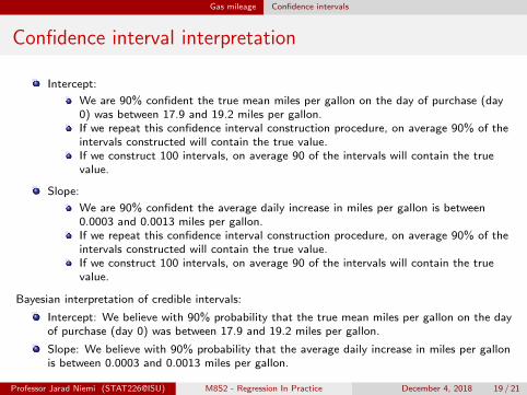
Gas mileage Confidence intervals
Confidence interval interpretation
Intercept:
We are 90% confident the true mean miles per gallon on the day of purchase (day0) was between 17.9 and 19.2 miles per gallon.If we repeat this confidence interval construction procedure, on average 90% of theintervals constructed will contain the true value.If we construct 100 intervals, on average 90 of the intervals will contain the truevalue.
Slope:
We are 90% confident the average daily increase in miles per gallon is between0.0003 and 0.0013 miles per gallon.If we repeat this confidence interval construction procedure, on average 90% of theintervals constructed will contain the true value.If we construct 100 intervals, on average 90 of the intervals will contain the truevalue.
Bayesian interpretation of credible intervals:
Intercept: We believe with 90% probability that the true mean miles per gallon on the dayof purchase (day 0) was between 17.9 and 19.2 miles per gallon.
Slope: We believe with 90% probability that the average daily increase in miles per gallonis between 0.0003 and 0.0013 miles per gallon.
Professor Jarad Niemi (STAT226@ISU) M8S2 - Regression In Practice December 4, 2018 19 / 21

Gas mileage Hypothesis tests
Hypothesis tests
JMP reports two p-values:
These correspond to the hypothesis tests
Intercept H0 : β0 = 0 vs Ha : β0 6= 0day H0 : β1 = 0 vs Ha : β1 6= 0
To obtain the one-sided p-values, you need to divided the p-value in halfand, if the alternative is not consistent with the estimate, subtract from 1.Example one-sided p-values are
Hypotheses p-valueH0 : β0 = 0 vs Ha : β0 > 0 < 0.0001H0 : β1 = 0 vs Ha : β1 < 0 0.9979
Professor Jarad Niemi (STAT226@ISU) M8S2 - Regression In Practice December 4, 2018 20 / 21
Gas mileage Hypothesis tests
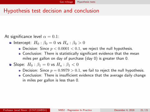
Hypothesis test decision and conclusion
At significance level α = 0.1:
Intercept: H0 : β0 = 0 vs Ha : β0 > 0
Decision: Since p < 0.0001 < 0.1, we reject the null hypothesis.Conclusion: There is statistically significant evidence that the meanmiles per gallon on day of purchase (day 0) is greater than 0.
Slope: H0 : β1 = 0 vs Ha : β1 < 0
Decision: Since p = 0.9979 > 0.1, we fail to reject the null hypothesis.Conclusion: There is insufficient evidence that the average daily changein miles per gallon is less than 0.
Professor Jarad Niemi (STAT226@ISU) M8S2 - Regression In Practice December 4, 2018 21 / 21