machine condition prognosis based on regression trees and one-step-ahead prediction

ARTICLE IN PRESS

Mechanical Systemsand

Signal Processing

0888-3270/$ - se

doi:10.1016/j.ym

�CorrespondE-mail addr

Mechanical Systems and Signal Processing 22 (2008) 1179–1193

www.elsevier.com/locate/jnlabr/ymssp

Machine condition prognosis based on regression trees andone-step-ahead prediction

Van Tung Trana, Bo-Suk Yanga,�, Myung-Suck Oha, Andy Chit Chiow Tanb

aSchool of Mechanical Engineering, Pukyong National University, San 100, Yongdang-dong, Nam-gu, Busan 608-739, South KoreabSchool of Mechanical, Manufacturing and Medical Engineering, Queensland University of Technology, G.P.O. Box 2343,

Brisbane, Qld 4001, Australia

Received 2 August 2007; received in revised form 11 November 2007; accepted 13 November 2007

Available online 19 November 2007

Abstract

Predicting the degradation of working conditions of machinery and trending of fault propagation before they reach the

alarm or failure threshold is extremely important in industry to fully utilize the machine production capacity. This paper

proposes a method to predict the future conditions of machines based on one-step-ahead prediction of time-series

forecasting techniques and regression trees. In this study, the embedding dimension is firstly estimated in order to

determine the necessarily available observations for predicting the next value in the future. This value is subsequently

utilized for the predictor which is generated by using regression tree technique. Real trending data of low methane

compressor acquired from condition monitoring routine are employed for evaluating the proposed method. The results

indicate that the proposed method offers a potential for machine condition prognosis.

r 2007 Elsevier Ltd. All rights reserved.

Keywords: Embedding dimension; Regression trees; Prognosis; Time-series forecasting

1. Introduction

Unexpected catastrophic failures of machine that lead to a costly maintenance or even human casualties canbe avoided with the proviso that the machine is appropriately maintained. Traditional maintenance strategiescommonly used in industry consist of corrective maintenance and preventive maintenance. The former means‘‘fix it when it breaks,’’ i.e., maintenance is carried out after a breakdown or when an obvious fault hasoccurred, whilst the latter is carried out in order to prevent equipment breakdown by performing repair,service, or replacing components at a fixed schedule. Even though preventive maintenance plans increase thereliability of machine, they are costly due to the frequent replacements of the expensive components before theend of their lives and the reduction of the availability of the machine’s productive capability. Therefore,the strategies of traditional maintenance are not adequate to fulfill the needs of expensive and high availabilityof industrial systems.

e front matter r 2007 Elsevier Ltd. All rights reserved.

ssp.2007.11.012

ing author. Tel.: +8251 620 1604; fax: +82 51 620 1405.

ess: [email protected] (B.-S. Yang).

www.elsevier.com/locate/jnlabr/ymssp

dx.doi.org/10.1016/j.ymssp.2007.11.012

mailto:[email protected]

ARTICLE IN PRESSV.T. Tran et al. / Mechanical Systems and Signal Processing 22 (2008) 1179–11931180

Condition-based maintenance (CBM) which involves prognostic module is an alternative maintenancestrategy that allows the machine to operate continuously until symptoms of a failure are detected. Prognosis isthe ability to access the current state, forecast the future state, and predict the time-to-failure or the remaininguseful life (RUL) of a failing components or subsystems. The RUL is the time left for the normal operation ofmachine before the breakdown occurs or machine condition reaches the critical failure value. Prognosis is alsoused to produce warning when the machine condition reaches the predetermined setup alarm or critical failurethreshold. Furthermore, it can be used for running repairs periodically in manufacturing facilities and fault-tolerant control [1]. Due to the benefits mentioned above, prognosis has been extensively researched with focuson CBM in the recent time.

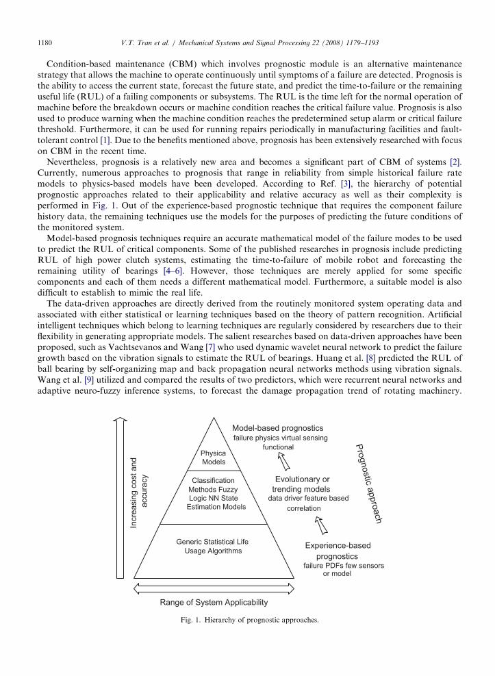
Nevertheless, prognosis is a relatively new area and becomes a significant part of CBM of systems [2].Currently, numerous approaches to prognosis that range in reliability from simple historical failure ratemodels to physics-based models have been developed. According to Ref. [3], the hierarchy of potentialprognostic approaches related to their applicability and relative accuracy as well as their complexity isperformed in Fig. 1. Out of the experience-based prognostic technique that requires the component failurehistory data, the remaining techniques use the models for the purposes of predicting the future conditions ofthe monitored system.

Model-based prognosis techniques require an accurate mathematical model of the failure modes to be usedto predict the RUL of critical components. Some of the published researches in prognosis include predictingRUL of high power clutch systems, estimating the time-to-failure of mobile robot and forecasting theremaining utility of bearings [4–6]. However, those techniques are merely applied for some specificcomponents and each of them needs a different mathematical model. Furthermore, a suitable model is alsodifficult to establish to mimic the real life.

The data-driven approaches are directly derived from the routinely monitored system operating data andassociated with either statistical or learning techniques based on the theory of pattern recognition. Artificialintelligent techniques which belong to learning techniques are regularly considered by researchers due to theirflexibility in generating appropriate models. The salient researches based on data-driven approaches have beenproposed, such as Vachtsevanos and Wang [7] who used dynamic wavelet neural network to predict the failuregrowth based on the vibration signals to estimate the RUL of bearings. Huang et al. [8] predicted the RUL ofball bearing by self-organizing map and back propagation neural networks methods using vibration signals.Wang et al. [9] utilized and compared the results of two predictors, which were recurrent neural networks andadaptive neuro-fuzzy inference systems, to forecast the damage propagation trend of rotating machinery.

Pro

gnostic

appro

ach

Incre

asin

g c

ost and

accu

racy

Model-based prognostics

Evolutionary or

trending models

Experience-based

prognostics

Range of System Applicability

failure physics virtual sensing

functional

data driver feature based

correlation

failure PDFs few sensorsor model

Physica

Models

Classification

Methods Fuzzy

Logic NN State

Estimation Models

Generic Statistical Life

Usage Algorithms

Fig. 1. Hierarchy of prognostic approaches.

ARTICLE IN PRESSV.T. Tran et al. / Mechanical Systems and Signal Processing 22 (2008) 1179–1193 1181

A hybrid approach of fuzzy logic and neural networks was employed to predict the RUL of bearings of smalland medium size induction motors [10].

Time-series prediction is a problem encountered in many fields from engineering (predictive control ofindustrial processes) to finance (forecasting returns of shares or stock markets). Models and predictionmethodologies have been proposed by a large community of researchers. For examples, Thissen et al. [11]applied three methods, namely, support vector machines, recurrent neural networks and autoregressivemoving average for times-series which predicted the process chemo metrics in field. Dulakshi et al. [12]employed artificial neural networks on time-series to predict river flow. Simon et al. [13] used self-organizingmaps algorithm to predict the missing value in CATS benchmark dataset.

The problems to be dealt with when predicting the future value is how many steps (time delays) areappropriate for obtaining the best performance? In time-series forecasting techniques, one-step-ahead ormulti-step-ahead prediction is frequently used. One-step-ahead or multi-step-ahead prediction implies that thepredictor utilizes the available observations to forecast one value or multiple values at the definite future time.According to Wang [1], the more the steps ahead is, the less reliable the forecasting operation is because multi-step prediction is associated with multiple one-step operations. This issue will be discussed further in theexperiments and results section.

Another problem is how many essential observations (inputs) are used for forecasting the future value,so-called embedding dimension d. The value of d should be chosen large enough for the predictor toestimate accurately the future value of machine condition and not too large to avoid the unnecessaryincrease in computational complexity. False nearest neighbor method (FNN) [14] and Cao’s method [15]are commonly used to determine the embedding dimension. However, FNN method depends on thechosen parameters wherein different values lead to different results. Furthermore, FNN method alsodepends on the number of available observations and is sensitive to additional noise. Cao’s methodovercomes the shortcomings of the FNN approach; and therefore, it is chosen in this study. After determiningthe embedding dimension d, the predictor is considered subsequently. Classification and regressiontree (CART) [16] is widely implemented in machine fault diagnosis. In the prediction techniques,regression tree and its extensions are applied to forecast the short-term load of the power system [17,18]with excellent performance. Hence, regression tree is proposed as a predictor for machine prognosis inthis paper.

2. Background knowledge

2.1. Determine the embedding dimension

Assuming a time-series of x1, x2,y, xN. The time delay vector constructed from this time-series is defined asfollows:

yiðdÞ ¼ ½xi;xiþt; . . . ; xiþðd�1Þt�; i ¼ 1; 2; . . . ;N � ðd � 1Þt, (1)

where t is the time delay and d is the embedding dimension. Defining the quantity as follows:

aði; dÞ ¼yiðd þ 1Þ � ynði;dÞðd þ 1Þ��

yiðdÞ � ynði;dÞðdÞ�� , (2)

where || � || is the Euclidian distance and is given by the maximum norm, yi(d) means the ith reconstructedvector and n(i,d) is an integer, so that yn(i, d)(d) is the nearest neighbor of yi(d) in the embedding dimension d. Inorder to avoid the problems encountered in FNN method, a new quantity is defined as the mean value of alla(i, d)’s:

EðdÞ ¼1

N � dt

XN�dt

i¼1

aði; dÞ: (3)


E(d) is only dependent on the dimension d and the time delay t. To investigate its variation from d to d+1,the parameter E1 is given by

E1ðdÞ ¼Eðd þ 1Þ

EðdÞ. (4)

By increasing the value of d, the value E1(d) is also increased and it stops increasing when the time-seriescomes from a deterministic process. If a plateau is observed for dXd0 then d0+1 is the minimum embeddingdimension.

The Cao’s method also introduced another quantity E2(d) to overcome the problem in practicalcomputations where E1(d) is slowly increasing or has stopped changing if d is sufficiently large:

E2ðdÞ ¼Enðd þ 1Þ

EnðdÞ, (5)

where

EnðdÞ ¼1

N � dt

XN�dt

i¼1

xiþdt � xnði;dÞþdt�� : (6)

According to Ref. [15], for purely random process, E2(d) is independent of d and equal to 1 for any of d.However, for deterministic time-series, E2(d) is related to d. Consequently, there must exist some d’s so thatE2(d) 6¼1.

2.2. Regression trees

CART method has been extensively developed by Breiman et al. [16] for classification or regressionpurpose depending on the response variable which is either categorical or numerical. In this study,CART is utilized to build up a regression tree model. Beginning with an entire data set, a binary tree isconstructed with the repeated splits of the subsets into two descendant subsets according to independentvariables. The goal is to produce subsets of the data which are as homogeneous as possible with respect to theresponse variables. Regression tree in CART is built by using the following two processes: tree growing andtree pruning.

2.2.1. Tree growing

Let L be a learning sample of size n, and it comprises n couples of observations (y1, x1),y, (yn, xn) wherexi ¼ ðx1i

; . . . ;xdiÞ is a set of independent variables and yiAR is a response associated with xi. The objective of

regression tree is to predict the values of response variables y ¼ (y1,y, yn) derived from the set of independentvariables (x1,y, xn). In order to build the tree, learning sample L is partitioned into two subsets by binarysplit. Splits are formed by using the inequality condition between criterion and value of independent variables.The result of this splitting is to move the couples (y, x) to left or right nodes containing more homogeneousresponses. This process is repeated until the terminal nodes are achieved. The predicted response at eachterminal node t is estimated by the average yðtÞ of the n(t) values y contained in that terminal node. The finalstructure of a binary tree T is shown in Fig. 2.

The split selection at any internal node t is chosen according to the node impurity that is measured bywithin-node sum of squares. The within-node sum of squares is the squared difference between the predictedresponse and observed response:

RðtÞ ¼1

n

Xyi ;xi2t

yi � yðtÞ2 (7)

and

yðtÞ ¼1

nðtÞ

Xyi ;xi2t

yi: (8)

ARTICLE IN PRESS

t1

t2

t 4 t5

t3

t 6 t 7

t8 t9

Root node

xi < a xi a

)( 4ty

Internal

node

Terminal

node

)( 6ty

)( 8ty )( 9ty

)( 5ty

≥

Fig. 2. Binary regression tree.

V.T. Tran et al. / Mechanical Systems and Signal Processing 22 (2008) 1179–1193 1183

When a split is performed, two subsets of observations tL and tR are obtained. The optimum split s* at nodet is obtained from the set of all splitting candidates S in order that it qualifies:

DRðs�; tÞ ¼ maxDRðs; tÞ; s 2 S

DRðs; tÞ ¼ RðtÞ � RðtLÞ � RðtRÞ;(9)

where R(tL) and R(tR) are sums of squares of the left and right subsets, respectively.The tree gained in tree growing process has many terminal nodes that lead to increase precision in

estimating of the responses. However, the tree with many terminal nodes is frequently too complicated andoverfitting is highly probable. Consequently, it should be pruned back to select the best tree.

2.2.2. Tree pruning

Let Tmax denote tree built on the sample L and T denote a sub-tree attained from Tmax by successivelyremoving the nodes. Pruning a tree allows to decrease the size of Tmax; therefore, T is smaller than Tmax. Theresult of pruning process will be a decreasing sequence of trees:

Tmax4T14 � � �4Tk ¼ ft1g, (10)

where {t1} denotes the root of tree. Along with the sequence of pruned trees, a corresponding sequence ofvalue a is found:

0 ¼ a1oa2o � � �oakoakþ1o � � �oaK , (11)

where aX0 is the cost parameter which weights the number of terminal node. For kX1, the tree Tk is thesmallest sub-tree that minimizes the error-complexity for interval akoaoak+1, and T(a) ¼ T(ak) ¼ Tk.

The error-complexity is defined as

RaðTÞ ¼ RðTÞ þ a ~T�� , (12)

where RðTÞ ¼ ð1=nÞPt2 ~T

Pðyi ;xiÞ2t

ðyi � yðtÞÞ2 is the total within-node sum of squares, ~T is the set of current nodes

of T and j ~T j is the number of terminal nodes in T.Tree pruning process is performed by the following procedure:

Step 1: At every internal node, an error-estimation is found for the number of descendant subtrees.Step 2: Using the error-estimation attained at step 1, the internal node with the smallest error is replaced byterminal node.Step 3: The algorithm terminates if all the internal nodes have converged to a terminal node. Otherwise, itreturns to step 1.


The best tree is chosen when both the error-complexity and the error-estimation are minimized. Theminimum error-estimation could be obtained by using the largest tree, but this increases the error-complexity.Therefore, the trade-off between those two criterions should be considered. There are two possible methods toaccomplish this. One is through the use of independent test samples and the other is cross-validation. In thisstudy, cross-validation method is used to determine the error-estimation.

2.2.3. Cross-validation for selecting the best tree

The learning sample L is randomly divided into V mutually exclusive data sets L1,y,Lv. It is the best toensure that all the V learning samples are of the same size or nearly the same. Let the learning sample L(v) bethe vth learning sample represented by L(v)

¼ L�Lv, v ¼ 1,y,V. L(v) is used as a learning sample formodel building and Lv is reserved as a testing sample for determining the error-estimation of the model.Each learning sample is used to grow a large tree and to get the corresponding sequence of pruned subtrees.Thus, a sequence of trees T(v)(a) that represents the minimum error-complexity trees for given values of a isachieved.

Simultaneously, the entire learning sample L is also employed to grow a large tree and to get the sequence ofsubtrees Tk with the corresponding sequence of ak. Define a0k ¼

ffiffiffiffiffiffiffiffiffiffiffiffiffiffiakakþ1p

as the geometric midpoint of theinterval [ak, ak+1]. Use d

ðvÞk ðxÞ to denote the prediction corresponding to the tree T ðvÞða0kÞ. The cross-validation

which estimates for the error-estimation is given:

RCV ðTkða0kÞÞ ¼1

n

XV

v¼1

Xðyi ;xiÞ2Lv

ðyi � dðvÞk ðxiÞÞ

2. (13)

From each case of the testing sample Lv with dðvÞk ðxÞ, a predicted response is attained, and then the squared

difference is calculated between the predicted response and the actual response. This process is repeated forevery testing sample. The average value of these errors is taken to determine the error-estimation of a treebased on values of RCV.

The standard error of cross-validation is obtained by using

SEðRCVðTkÞÞ ¼

ffiffiffiffis2

n

r(14)

and

s2 ¼1

n

Xxi ;yi

ðyi � dðvÞk ðxiÞÞ

2� R

CVðTkÞ

h i2: (15)

The subtree that has the smallest error is found and denoted by T0. Finally, the best tree T�k is selectedsuch that

RCVðT�kÞR

CV

minðT0Þ þ SEðRCV

minðT0ÞÞ

RCV

minðT0Þ ¼ minfRCVðTkÞg:

(16)

3. Proposed system

Normally, when a fault occurs in a machine, the conditions of machine can be identified by the change invibration amplitude. In order to predict the future state of the machine conditions based on available vibrationdata, regression tree predictor is used. The proposed system is shown in Fig. 3. This system consists of fourprocedures sequentially: data acquisition, data splitting, training-validating model and predicting. The role ofeach procedure is explained as follows:

Step 1. Data acquisition: The use of vibration data from the machine for trending. It consists of historicaldata and vibration data during the running process of the machine until faults occur.

ARTICLE IN PRESS

Trending data of machine

Splitting data

Training dataTesting data

Determine embeddingdimension

Building model

Validating model

Good model

Yes

No

Yes

No

Predicting

Good results

Prognosis

Cao,s

method

Regression

tree

OneStep aheadprediction

Fig. 3. Proposed system for machine fault prognosis.

V.T. Tran et al. / Mechanical Systems and Signal Processing 22 (2008) 1179–1193 1185

Step 2. Data splitting: The trending data is split into two parts: training data and testing data. Differentdata is used for different purposes in the prognosis system. Training data is used for building the modelwhilst testing data is utilized to test the validated model.Step 3. Training-validating: This procedure includes the following sub-procedures: determining theembedding dimension based on Cao’s method, building the model and validating the model. Validatingmodel is used for measuring the performance capability of the model.Step 4. Predicting: This procedure uses one-step-ahead prediction to forecast the future value. Thepredicted result is measured by the error between predicted value and actual value in the testing data. If theprediction is successful, the result obtained from this procedure is the prognosis system.

4. Experiments and results

The proposed method is applied to real system to predict the trending data of a low methane compressor.This compressor shown in Fig. 4 is driven by a 440 kW motor, 6600V, 2 pole and operating at speed of3565 rpm. The other information of system is summarized in Table 1.

ARTICLE IN PRESS

CMS Offline monitoring (100mV/g acceleration)

Male rotor vertical Male rotor horizontal

Suction vertical, horizontal,axial Male rotor axial

Symptom sensing

Motor DE/NDE horizontal

Motor DE/NDE vertical

Motor DE/NDE axial

CMS Off-line monitoring (100mV/g acceleration

(Only horizontal)

Fig. 4. Low methane compressor: wet screw type.

Table 1

Description of system

Electric motor Compressor

Voltage 6600V Type Wet screw

Power 440 kW Lobe Male rotor (4 lobes)

Pole 2 pole Female rotor (6 lobes)

Bearing NDE: #6216, DE: #6216 Bearing Thrust: 7321 BDB

RPM 3565 rpm Radial: sleeve type

0 200 400 600 800 1000 12000

0.2

0.4

0.6

0.8

1

1.2

1.4

Time

Acce

lera

tio

n (

g)

Fig. 5. The entire of peak acceleration data of low methane compressor.

V.T. Tran et al. / Mechanical Systems and Signal Processing 22 (2008) 1179–11931186


The data applied in this study is peak acceleration and envelope acceleration trending data. The trendingdata was recorded from August 2005 to November 2005. The average sampling rate was 6 h during the dataacquisition process. This data approximately consists of 1200 data points shown in Figs. 5 and 6. This datacontains information of machine history with respect to time sequence (vibration amplitude). Consequently, itcan be seen as time-series data. The proposed method is employed to predict the future condition of vibrationamplitude based on the past and current states.

0

Accele

ration (

g)

200 400 600 800 1000 12000

0.5

1

1.5

2

2.5

3

Time

Fig. 6. The entire of envelope acceleration data of low methane compressor.

Fig. 7. The faults of main bearings of compressor.


The machine is in normal condition during the time correlated with the first 300 points. After that time, thecondition of machine suddenly changes. It indicates that there are some faults occurring in this machine. Thesefaults were the damages of main bearings of compressor (notation Thrust: 7321 BDB) due to the insufficientlubrication. Consequently, the babbitt surfaces of these bearings were overheated and delaminated as depictedin Fig. 7.

With the aim of forecasting the change of machine condition, the first 300 points were used to train thesystem and the following 150 points were employed for testing system. In order to evaluate the predicting

0 50 100 150 200 250 300

0.34

0.36

0.38

0.4

0.42

0.44

0.46

Time

Acce

lera

tion (

g)

RMSE = 0.0006219

Actual

Predicted

Fig. 8. Training and validating results of peak acceleration data (the first 300 points).

Acce

lera

tio

n (

g)

1.4

1.2

1

0.8

0.6

0.4

0.2

00 50 100 150

Time

Actual

Predicted

Fig. 9. Predicted results of peak acceleration data.


performance, the root-mean square error (RMSE) is utilized as follows:

RMSE ¼

ffiffiffiffiffiffiffiffiffiffiffiffiffiffiffiffiffiffiffiffiffiffiffiffiffiffiffiffiffiPNi¼1ðyi � yiÞ

2

N

s, (17)

where N represents the total number of data points in the test set, yi is actual value in training set or test set,and yi represents the predicted value of the model.

Because the sampling rate was 6 h in data acquisition process, it is large enough to make the decisionwhether to stop or to continue the operation of this machine when its conditions reach the predeterminedsetup alarm or critical failure threshold. That is the reason for choosing one-step-ahead prediction in thisstudy. Therefore, the time delay value is also chosen as t ¼ 1 in all datasets. Furthermore, the number of cases

Acce

lera

tio

n (

g)

0.8

0.75

0.7

0.65

0.6

0.55

0.5

0.45

0.4

0.35350 400 450 500 550 600 650 700 750 800

Time

Fig. 10. Peak acceleration of low methane compressor.

0 5 10 150

0.2

0.4

0.6

0.8

1

1.2

Dimension, d

E1

E2

E1(d

), E

2(d

)

Fig. 11. The values of E1 and E2 of peak acceleration data of low methane compressor.


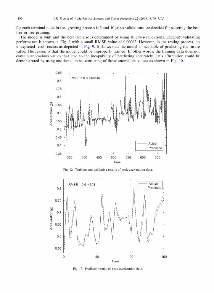
for each terminal node in tree growing process is 5 and 10 cross-validations are decided for selecting the besttree in tree pruning.

The model is built and the best tree size is determined by using 10 cross-validations. Excellent validatingperformance is shown in Fig. 8 with a small RMSE value of 0.00062. However, in the testing process, anunexpected result occurs as depicted in Fig. 9. It shows that the model is incapable of predicting the futurevalue. The reason is that the model could be improperly trained. In other words, the training data does notcontain anomalous values that lead to the incapability of predicting accurately. This affirmation could bedemonstrated by using another data set consisting of those anomalous values as shown in Fig. 10.

350 400 450 500 550 600 650

0.35

Acce

lera

tio

n (

g)

0.4

0.45

0.5

0.55

0.6

0.65

0.7

0.75

0.8

0.85

Time

RMSE = 0.00060146

Actual

Predicted

Fig. 12. Training and validating results of peak acceleration data.

Acce

lera

tio

n (

g)

0.8

0.75

0.7

0.65

0.6

0.55

0 50

Time

100 150

Actual

PredictedRMSE = 0.014394

Fig. 13. Predicted results of peak acceleration data.


Theoretically, the minimum embedding dimension is chosen as E1(d) obtains a plateau. In Fig. 11, theembedding dimension is chosen as 6 for the reason that the values of E1(d) reaches its saturation. This value isused for regression tree predictor. Figs. 12 and 13 are the validating and testing model, respectively. Thetraining and validating results of peak acceleration data are almost identical as shown in Fig. 12, with a verysmall RMSE value of 0.000601. In the testing process, even though the model cannot predict accurately themachine condition, the RMSE value shown in Fig. 13 is 0.0143 which is acceptable.

Fig. 14 performs the trending data of envelope acceleration of low methane compressor. By using the similarprocesses, i.e., estimating embedding dimension (this value is 6 shown in Fig. 15), validating model and testingmodel by using independent data set are, respectively, carried out and the final results are performed in

Acce

lera

tio

n (

g)

450400350300250200150100500.5

1

1.5

2

2.5

3

Time

Fig. 14. Data trending of envelope acceleration of low methane compressor.

E1(d

), E

2(d

)

1510500

0.2

0.4

0.6

0.8

1

Dimension, d

E1

E2

Fig. 15. The values of E1 and E2 of envelope acceleration data.


Figs. 16 and 17. The training and validating results closely resemble the actual data with a RMSE error of0.000291 as shown in Fig. 16. Although the predictor is incapable of predicting the machine conditionprecisely, it can closely track the changes of trending condition of machine with a small error of 0.06 as shownin Fig. 17.

50 100 150 200 250 300 350

0.5

1

1.5

2

2.5

3

Number of data

Accele

ration (

g)

RMSE = 0.00029121Actual

Predicted

Fig. 16. Training and validating results of envelope acceleration data.

Accele

ration (

g)

2.5

2

1.5

1

0 50

Time

100 150

Actual

PredictedRMSE = 0.060354

Fig. 17. Predicted results of envelope acceleration data.


5. Conclusions

Machine condition prognosis is extremely significant in foretelling the degradation working condition andtrends of fault propagation before they reach the alarm or failure threshold. In this study, the machineprognosis based on one-step-ahead of time-series techniques and regression trees has been investigated. Theproposed method is validated by predicting future state condition of a low methane compressor whereinthe peak acceleration and envelope acceleration have been examined. Using 10 cross-validations to find theoptimum tree size and an embedded dimension of 6, the results give a prediction error of 1.43% with peakacceleration data, and 6% with the enveloped acceleration data. These errors are small in statistical sense. Theresults confirm that the proposed method offers a potential for machine condition prognosis with one-step-ahead prediction.

References

[1] W. Wang, An adaptive predictor for dynamic system forecasting, Mechanical Systems and Signal Processing 21 (2007) 809–823.

[2] J. Luo, M. Namburu, K. Pattipati, L. Qiao, M. Kawamoto, S. Chigusa, Model-based prognostic techniques, in: AUTOTESTCON

Proceedings of the IEEE Systems Readiness Technology Conference, 22–25 September 2003, pp. 330–340.

[3] G. Vachtsevanos, F. Lewis, M. Roemer, A. Hess, B. Wu, Intelligent Fault Diagnosis and Prognosis for Engineering System, Wiley,

2006.

[4] M. Watson, C. Byington, D. Edwards, S. Amin, Dynamic modeling and wear-based remaining useful life prediction of high power

clutch systems, Tribology Transactions 48 (2005) 208–217.

[5] M. Luo. D. Wang, M. Pham, C.B. Low, J.B. Zhang, D.H. Zhang, Y.Z. Zhao, Model-based fault diagnostis/prognosis for wheeled

mobile robots: a review, in: Proceedings of the 32nd Annual Conference of IEEE, Industrial Electronics Society, 6–10 November

2005, pp. 2267–2272.

[6] Y. Li, T.R. Kurfess, S.Y. Liang, Stochastic prognostics for rolling element bearings, Mechanical Systems and Signal Processing 14

(2000) 747–762.

[7] G. Vachtsevanos, P. Wang, Fault prognosis using dynamic wavelet neural networks, in: AUTOTESTCON Proceedings of the IEEE

Systems Readiness Technology Conference, 22–23 August 2001, pp. 857–870.

[8] R. Huang, L. Xi, X. Li, C.R. Liu, H. Qiu, J. Lee, Residual life prediction for ball bearings based on self-organizing map and back

propagation neural network methods, Mechanical Systems and Signal Processing 21 (2007) 193–207.

[9] W.Q. Wang, M.F. Golnaraghi, F. Ismail, Prognosis of machine health condition using neuro-fuzzy system, Mechanical System and

Signal Processing 18 (2004) 813–831.

[10] B. Satish, N.D.R. Sarma, A fuzzy BP approach for diagnosis and prognosis of bearing faults in induction motors, IEEE Power

Engineering Society General Meeting 3 (2005) 2291–2294.

[11] U. Thissen, R. van Brakel, A.P. de Weijer, W.J. Melssen, L.M.C. Buydens, Using support vector machines for time series predicting,

Chemometrics and Intelligent Laboratory Systems 69 (2003) 35–49.

[12] S.K. Dulakshi Karunasinghea, S.-Y. Liongb, Chaotic time series prediction with a global model: artificial neural network, Journal of

Hydrology 323 (2006) 92–105.

[13] G. Simon, J.A. Lee, M. Cottrell, M. Verleysen, Forecasting the CATS benchmark with the double vector quantization,

Neurocomputing 70 (2007) 2400–2409.

[14] M.B. Kennel, R. Brown, H.D.I. Abarbanel, Determining embedding dimension for phase-space reconstruction using a geometrical

construction, Physical Review A 45 (1992) 3403–3411.

[15] L. Cao, Practical method for determining the minimum embedding dimension of a scalar time series, Physica D 110 (1997) 43–50.

[16] L. Breiman, J.H. Friedman, R.A. Olshen, C.J. Stone, Classification and Regression Trees, Chapman & Hall, 1984.

[17] J. Yang, J. Stenzel, Short-term load forecasting with increment regression tree, Electric Power Systems Research 76 (2006) 880–888.

[18] H. Moti, N. Kosemura, K. Ishiguro, T. Kondo, Short-term load forecasting with fuzzy regression tree in power systems, system man

and cybernetics, IEEE International Conference 3 (2001) 1948–1953.

machine condition prognosis based on regression trees and one-step-ahead prediction

Documents