machine intelligence laboratory
TRANSCRIPT

� ��������� ������������� �������������������! "��#$�&%'���� ( �&�)�* "�
+-,/.10!243�57698:3<;98>=
?A@CBEDGFGHJI KML�NOF>PQPSR<TGR
DGUJIVR�WYXGXAZ
[]\C^`_baM_c_edCfhgiakjeje^`l�jnmojn\C^qpsrCaut�^`vb_eakjxw�mzyJ{}|�g~fCveaulC��^qaur���|zvbjnaM|��>y�dh�u���ug�^`r�jm�y�jn\C^�vb^`��dCauve^`g�^�r�je_cy�m�v}je\C^�lC^`��ve^`^qm�y��/mY��jnm�v�m�yV�J\Cau�um�_em��h\�w

� �$#'����� ���
Language models are computational techniques and structures that describe word sequences produced byhuman subjects, and the work presented here considers primarily their application to automatic speech-recognition systems. Due to the very complex nature of natural languages as well as the need for robustrecognition, statistically-based language models, which assign probabilities to word sequences, haveproved most successful.
This thesis focuses on the use of linguistically defined word categories as a means of improving theperformance of statistical language models. In particular, an approach that aims to capture both generalgrammatical patterns, as well as particular word dependencies, using different model components isproposed, developed and evaluated.
To account for grammatical patterns, a model employing variable-length n-grams of part-of-speech wordcategories is developed. The often local syntactic patterns in English text are captured conveniently bythe n-gram structure, and reduced sparseness of the data allows larger � to be employed. A techniquethat optimises the length of individual n-grams is proposed, and experimental tests show it to lead toimproved results. The model allows words to belong to multiple categories in order to cater for differentgrammatical functions, and may be employed as a tagger to assign category classifications to new text.
While the category-based model has the important advantage of generalisation to unseen word se-quences, it is by nature not able to capture relationships between particular words. An experimentalcomparison with word-based n-gram approaches reveals this ability to be important to language modelquality, and consequently two methods allowing the inclusion of word relations are developed.
The first method allows the incorporation of selected word n-grams within a backoff framework. Thenumber of word n-grams added may be controlled, and the resulting tradeoff between size and accuracyis shown to surpass that of standard techniques based on n-gram cutoffs. The second technique ad-dresses longer-range word-pair relationships that arise due to factors such as the topic or the style of thetext. Empirical evidence is presented demonstrating an approximately exponentially decaying behaviourwhen considering the probabilities of related words as a function of an appropriately defined separatingdistance. This definition, which is fundamental to the approach, is made in terms of the category assign-ments of the words. It minimises the effect syntax has on word co-occurrences while taking particularadvantage of the grammatical word classifications implicit in the operation of the category model. Sinceonly related words are treated, the model size may be constrained to reasonable levels. Methods bymeans of which related word pairs may be identified from a large corpus, as well as techniques allow-ing the estimation of the parameters of the functional dependence, are presented and shown to lead toperformance improvements.
The proposed combination of the three modelling approaches is shown to lead to considerable perplex-ity reductions, especially for sparse training sets. Incorporation of the models has led to a significantimprovement in the word error rate of a high-performance baseline speech-recognition system.

� �$�� "��]��� ��� #
This thesis is the result of my own original work, and where it draws on the work of others,this is acknowledged at the appropriate points in the text. This thesis has not been submittedin whole or in part for a degree at any other institution. Some of the work has been publishedpreviously in conference proceedings ([57], [60], [62]). The length of this thesis, includingappendices and footnotes, is approximately 43,000 words.

� ���$# ��� "�$� ��*( �*#����
First and foremost I would like to thank my supervisor, Phil Woodland. His experiencedopinion and sound advice have guided the course of this research to its successful conclu-sion, and with his consistent support I have already been able to publish and present parts ofthis research at respected conferences. It has been a privilege to work under his supervision.
Then I would like to express my gratitude to St. John’s College, who have provided finan-cial support in the form of a Benefactor’s Scholarship, without which my doctoral studieswould not have been possible. Furthermore I would like to acknowledge the generous ad-ditional funds provided by the Harry Crossley Foundation and the Cambridge UniversityEngineering Department, which have allowed me to present my research at conferences inAtlanta, Philadelphia and Munich.
I am very grateful to Claudia Arena, Selwyn Blieden, Anna Lindsay, Christophe Molina,Eric Ringger, Piotr Romanowski, and my sister Carola, for proofreading all or sections ofthis manuscript. Without their help, I could not have presented the result of my research as itappears here. Then I have been fortunate to spend many working hours with my colleagueshere in the Speech Laboratory, whom I thank for their continued assistance, good company,and for all that tea. Furthermore I owe a great deal to Patrick Gosling, Andrew Gee andCarl Seymour, the maintainers of the excellent computing facilities, without which thiswork would certainly not have been possible. The recognition experiments in this thesiswere accomplished using the Entropic Lattice and Language Modelling Toolkit, and I thankJulian Odell for his major contribution to the preparation of this software, which has madethe last phase of my research much simpler. Finally I would like to say how grateful I amto my family for their enduring support throughout the duration of my studies, and for theirunquestioning faith in my abilities.

Page i
Table of contents
1. Introduction 11.1. The speech recognition problem ��������������������������������������������������������������������������� 2
1.1.1. Preprocessing of the speech signal ����������������������������������������������������������������� 2
1.1.2. The acoustic model ��������������������������������������������������������������������������������������������� 2
1.1.3. The language model ������������������������������������������������������������������������������������������� 3
1.2. Dominant language modelling techniques ��������������������������������������������������������� 3
1.3. Scope of this thesis ����������������������������������������������������������������������������������������������������� 5
1.3.1. Modelling syntactic relations ��������������������������������������������������������������������������� 5
1.3.2. Modelling fixed short-range semantic relations ������������������������������������������� 5
1.3.3. Modelling long-range semantic relations ����������������������������������������������������� 6
1.4. Thesis organisation ��������������������������������������������������������������������������������������������������� 6
2. Overview of language modelling techniques 72.1. Perplexity ��������������������������������������������������������������������������������������������������������������������� 7
2.2. Equivalence mappings of the word history ����������������������������������������������������� 10
2.3. Probability estimation from sparse data ��������������������������������������������������������� 11
2.3.1. The Good-Turing estimate ����������������������������������������������������������������������������� 12
2.3.2. Deleted estimation ������������������������������������������������������������������������������������������� 16
2.3.3. Discounting methods ��������������������������������������������������������������������������������������� 17
2.3.3.1. Linear discounting ��������������������������������������������������������������������������������� 17
2.3.3.2. Absolute discounting ������������������������������������������������������������������������������� 18
2.3.4. Backing off to less refined distributions ����������������������������������������������������� 18
2.3.5. Deleted interpolation ��������������������������������������������������������������������������������������� 20
2.3.6. Modified absolute discounting ����������������������������������������������������������������������� 21
2.4. N-gram models ��������������������������������������������������������������������������������������������������������� 22
2.5. Category-based language models ����������������������������������������������������������������������� 24
2.5.1. Word categories ������������������������������������������������������������������������������������������������� 24
2.5.2. Automatic category membership determination ��������������������������������������� 26
2.5.3. Word groups and phrases ������������������������������������������������������������������������������� 28
Ph.D. dissertation, Thomas Niesler, Cambridge University, June 1997

Page ii
2.6. Longer-term dependencies ����������������������������������������������������������������������������������� 29
2.6.1. Pairwise dependencies ������������������������������������������������������������������������������������� 29
2.6.2. Cache models ��������������������������������������������������������������������������������������������������� 32
2.6.3. Stochastic decision tree based language models ��������������������������������������� 34
2.7. Domain adaptation ������������������������������������������������������������������������������������������������� 36
2.7.1. Specialisation to a target domain ����������������������������������������������������������������� 36
2.7.2. Mixtures of topic-specific language models ����������������������������������������������� 37
2.8. Language models for other applications ��������������������������������������������������������� 38
2.8.1. Character and handwriting recognition ������������������������������������������������������� 38
2.8.2. Machine translation ����������������������������������������������������������������������������������������� 38
2.8.3. Spelling correction ������������������������������������������������������������������������������������������� 39
2.8.4. Tagging ��������������������������������������������������������������������������������������������������������������� 39
3. Variable-length category-based n-grams 403.1. Introduction and overview ����������������������������������������������������������������������������������� 40
3.2. Structure of the language model ����������������������������������������������������������������������� 40
3.2.1. Estimating������������
��������������������������������������������������������������������������������������� 42
3.2.2. Estimating��������� ����
����������������������������������������������������������������������������������������� 44
3.2.3. Estimating���������������������� �
����������������������������������������������������������������������� 44
3.2.4. Beam-pruning ��������������������������������������������������������������������������������������������������� 47
3.2.5. Employing the language model as a tagger ����������������������������������������������� 47
3.3. Performance evaluation ����������������������������������������������������������������������������������������� 48
3.3.1. Tagging accuracy ��������������������������������������������������������������������������������������������� 48
3.3.1.1. Lexicon augmentation ��������������������������������������������������������������������������� 49
3.3.1.2. Beam pruning ������������������������������������������������������������������������������������������� 49
3.3.1.3. Tagging the Switchboard and WSJ corpora ��������������������������������������� 50
3.3.2. Constructing category trees ��������������������������������������������������������������������������� 51
3.3.3. Word-perplexity ����������������������������������������������������������������������������������������������� 54
3.4. Comparing word- and category-based models ��������������������������������������������� 55
3.4.1. Overall probability estimates ������������������������������������������������������������������������� 55
3.4.2. The effect of backoffs ������������������������������������������������������������������������������������� 56
3.4.3. Per-category analysis ��������������������������������������������������������������������������������������� 56
3.4.4. Per-n-gram analysis ����������������������������������������������������������������������������������������� 59
3.4.5. Robustness to domain-change ����������������������������������������������������������������������� 60
3.5. Summary and conclusion ������������������������������������������������������������������������������������� 61
Ph.D. dissertation, Thomas Niesler, Cambridge University, June 1997
Page iii
4. Word-to-category backoff models 62
4.1. Introduction ������������������������������������������������������������������������������������������������������������� 62
4.2. Exact model ��������������������������������������������������������������������������������������������������������������� 62
4.3. Approximate model ����������������������������������������������������������������������������������������������� 63
4.4. Model complexity : determining ��� ��������������������������������������������������������������� 66
4.4.1. Testing n-gram counts ������������������������������������������������������������������������������������� 66
4.4.2. Testing the effect on the overall probability ����������������������������������������������� 66
4.5. Model building procedure ����������������������������������������������������������������������������������� 67
4.6. Results ������������������������������������������������������������������������������������������������������������������������� 67
4.6.1. LOB corpus ������������������������������������������������������������������������������������������������������� 68
4.6.2. Switchboard corpus ����������������������������������������������������������������������������������������� 69
4.6.3. WSJ corpus ������������������������������������������������������������������������������������������������������� 70
4.7. Summary and conclusion ������������������������������������������������������������������������������������� 70
5. Word-pair dependencies in category-based language models 71
5.1. Introduction ������������������������������������������������������������������������������������������������������������� 71
5.2. Terminology ������������������������������������������������������������������������������������������������������������� 71
5.3. Probabilistic framework ��������������������������������������������������������������������������������������� 72
5.3.1. Estimating���
����������������������������������������������������������������������������������������������������� 74
5.3.2. Estimating � and � ������������������������������������������������������������������������������������������� 74
5.3.3. Typical estimates ��������������������������������������������������������������������������������������������� 76
5.4. Determining trigger-target pairs ����������������������������������������������������������������������� 76
5.4.1. First-pass ����������������������������������������������������������������������������������������������������������� 76
5.4.2. Second-pass ������������������������������������������������������������������������������������������������������� 79
5.4.3. Regulating memory usage ����������������������������������������������������������������������������� 80
5.4.4. Example pairs ��������������������������������������������������������������������������������������������������� 80
5.5. Perplexity results ����������������������������������������������������������������������������������������������������� 81
5.6. Discussion ����������������������������������������������������������������������������������������������������������������� 83
5.7. Summary and conclusion ������������������������������������������������������������������������������������� 84
Ph.D. dissertation, Thomas Niesler, Cambridge University, June 1997

Page iv
6. Word error rate performance 85
6.1. Language models in the recognition search ��������������������������������������������������� 85
6.1.1. N-best rescoring. ��������������������������������������������������������������������������������������������� 87
6.1.2. Lattice rescoring. ��������������������������������������������������������������������������������������������� 88
6.2. Recognition experiments ��������������������������������������������������������������������������������������� 88
6.2.1. Baseline results ������������������������������������������������������������������������������������������������� 88
6.2.2. Rescoring results ����������������������������������������������������������������������������������������������� 89
6.2.2.1. Category model ��������������������������������������������������������������������������������������� 89
6.2.2.2. Word-to-category backoff model ����������������������������������������������������������� 90
6.2.2.3. Category model with long-range correlations ��������������������������������� 90
6.2.2.4. Word-to-category backoff model with long-range correlations ����� 91
6.3. Summary and conclusion ������������������������������������������������������������������������������������� 91
7. Summary and conclusions 92
7.1. Review of conducted work ����������������������������������������������������������������������������������� 92
7.1.1. The category-based syntactic model ������������������������������������������������������������� 92
7.1.2. Inclusion of word n-grams ����������������������������������������������������������������������������� 93
7.1.3. Inclusion of long-range word-pair relations ����������������������������������������������� 94
7.2. Conclusion and topics for future investigation ��������������������������������������������� 94
7.2.1. Tagging ��������������������������������������������������������������������������������������������������������������� 94
7.2.2. Data-driven refinement of category definitions ����������������������������������������� 95
7.2.3. Punctuation ������������������������������������������������������������������������������������������������������� 95
7.2.4. Lattice rescoring ����������������������������������������������������������������������������������������������� 95
7.3. Final summary ��������������������������������������������������������������������������������������������������������� 95
8. References 96
Ph.D. dissertation, Thomas Niesler, Cambridge University, June 1997
Page v
A. Appendix : Major text corpora 102
B. Appendix : Leaving-one-out cross-validation 103
C. Appendix : Dealing with unknown words 105
D. Appendix : Experimental corpora and baselinelanguage models
107
D.1. Introduction ����������������������������������������������������������������������������������������������������������� 107
D.2. The LOB corpus ��������������������������������������������������������������������������������������������������� 107
D.2.1. Preprocessing ������������������������������������������������������������������������������������������������� 107
D.2.2. Corpus statistics ��������������������������������������������������������������������������������������������� 108
D.2.3. Baseline word-based n-gram models ������������������������������������������������������� 108
D.3. The Switchboard (SWBD) corpus ����������������������������������������������������������������� 109
D.3.1. Preprocessing ������������������������������������������������������������������������������������������������� 109
D.3.2. Corpus statistics ��������������������������������������������������������������������������������������������� 109
D.3.3. Baseline word-based n-gram models ������������������������������������������������������� 109
D.4. The Wall Street Journal (WSJ) corpus ��������������������������������������������������������� 110
D.4.1. Preprocessing ������������������������������������������������������������������������������������������������� 110
D.4.2. Corpus statistics ��������������������������������������������������������������������������������������������� 110
D.4.3. Baseline word-based n-gram models ������������������������������������������������������� 111
E. Appendix : LOB corpus word-categories 112
E.1. Part-of-speech tags found in the LOB corpus ��������������������������������������������� 112
E.2. Contactions and their part-of-speech tag assignments ��������������������������� 115
F. Appendix : OALD tag mappings 116
G. Appendix : Trigger approximations 117
G.1. First approximation ������������������������������������������������������������������������������������������� 117
G.2. Second approximation ��������������������������������������������������������������������������������������� 118
H. Appendix : The truncated geometric distribution 121
Ph.D. dissertation, Thomas Niesler, Cambridge University, June 1997

Chapter 1: Introduction Page 1
Chapter 1
Introduction
Research into language modelling aims to develop computational techniques and structures that de-scribe word sequences as produced by human subjects. Such models can be employed to deliver assess-ments of the correctness and plausibility of given samples of text, and have become essential tools inseveral research fields. The work in this thesis primarily considers their application to speech recogni-tion, which has developed into a major research area over the past 30 years. The current principal ob-jective is the development of large-vocabulary recognisers for natural, unconstrained, connected speech.Despite consistent progress, considerable advances are still necessary before widespread industrial ap-plication becomes feasible. However, the very broad spectrum of potential applications1 will ensure thatthis technology will gain extreme importance once it matures.
Two major approaches to the modelling of human language may be identified. The first relies on syn-tactic and semantic analyses of the sample text to determine the hierarchical sentence structure. Suchanalyses employ a set of rules to ascertain whether a sentence is permissible or not, and although it hasbeen possible to describe a significant proportion of English usage in this way, complete coverage hasremained elusive. This is due, at least in part, to the continuous changes taking place in a living language.Furthermore, utterances that are clearly not grammatical occur often in natural language, but cannot bedealt with by such analyses. This significant likelihood of failure under such naturally occurring cir-cumstances has led to infrequent use of the rule-based approach in speech recognition systems. Instead,a second approach based on statistical techniques with intrinsically greater robustness to grammaticalirregularities is usually taken. Such statistical language models assign to each word in an utterancea probability value according to its deemed likelihood within the context of the surrounding word se-quence. The probabilities are inferred from a large body of example text, referred to as the trainingcorpus. In this way the model may come to reflect language usage as found in practice, and not only itsgrammatical idealisation. Moreover, advantage may be taken of the recent vast increases in the amountof available training text, which now runs into hundreds of millions of words.
A speech-recognition system must find the most likely sentence hypothesis for each spoken utterance.When dealing with connected speech, not only are the words themselves unknown, but also their numberand boundaries in time. For large vocabularies, this leads to an extremely high number of possiblealternative segmentations of the acoustic signal into words. In this context, the language model evaluatesthe linguistic plausibility of partial or complete hypotheses. In conjunction with the remainder of therecognition system, this estimate assists in finding those hypotheses which are most likely to lead to thecorrect result, as well as those which may be discarded in order to limit the number to practical levels.
1Examples of such applications include: automatic dictation systems, hearing systems for the deaf, automated telephone enquiry, automatedteaching of foreign languages, and voice-control of electronic and computer equipment.
Ph.D. dissertation, Thomas Niesler, Cambridge University, June 1997
Chapter 1: Introduction Page 2
Although this work focuses on their application to speech-recognition systems, language models are im-portant components also in other areas2, such as handwriting recognition, machine translation, spellingcorrection, and part-of-speech tagging.
The following sections will describe the main elements of a speech recognition system, highlight therole of the language model, and outline the scope of the remainder of this thesis.
1.1. The speech recognition problem
In speech recognition, the aim is to find the most likely sequence of words � given the observed acousticdata � . This is achieved by finding that � which maximises the conditional probability
��� ������ . FromBayes rule,
��� ����� =��� ������� ��� ������ �� (1)
but since��� �� is constant for a given acoustic signal, an equivalent strategy is to find :
arg max��� � ��� ������� ��� ����� (2)
The acoustic component of the speech recogniser must compute��� ������� , whereas the language model
must estimate the prior probability of a certain sequence of words,��� ��� . Before focusing our attention
on the latter, we will present some background on the acoustic processing.
1.1.1. Preprocessing of the speech signal
Speech obtained from a microphone or recording device is in the form of an analogue electrical signal.This is processed into a form suitable for use within a speech-recognition system by a series of operationscommonly referred to collectively as the front end. Usually these steps include band-limiting the signal,sampling it, and then applying some spectral transformation to encode its frequency characteristics. Thislast step normally employs the short-term discrete Fourier transform, and a particular popular choice is toencode the speech as Mel-frequency cepstral coefficients [72], which capture the spectral characteristicsof the signal on a Mel-frequency scale. The resulting discrete-time sequence of observation vectors isthe output of the front-end, and is passed to the recognition algorithm.
1.1.2. The acoustic model
Central to every speech recognition system is a means of encoding the sounds comprising human speech.This has been most successfully achieved through the use of hidden Markov models (HMMs) [71], [94],although other approaches have also met with success [77]. By describing the observation vectors as aprobabilistic time series, the HMM takes the inherent natural variability of human speech characteristicsinto account. Given a set of examples of a particular sound in the form of the corresponding observationvector sequences � , the parameters of the model � may be adjusted to best represent this data in aprobabilistic sense, often by optimising
��� ������� . The model may consequently be employed to evalu-ate the likelihood of a new observation sequence with respect to its parameters, thus giving an indicationof how similar the new measurement is to those originally used to determine its parameters. This likeli-hood is used to make a statistical decision regarding the utterance to be recognised, as illustrated in the
2A brief overview of these is given in section 2.8.
Ph.D. dissertation, Thomas Niesler, Cambridge University, June 1997

Chapter 1: Introduction Page 3
following figure, which depicts a simple speech recognition system capable of distinguishing betweenthe words “hello” and “goodbye”.
Front-endpreprocessor
Acoustic model for"Hello"
Acoustic model for"Goodbye" �����������������������������������
�������������������������������������������������������������������������������������L
ikel
ihoo
d
"Hello"
Speech waveform
"Hello"
time
Observation vectors
Figure 1.1: A simple speech recognition system.
HMMs may either be trained to model entire words directly, or to model subword units (such asphonemes) which are concatenated to obtain words. The latter approach is usually adopted since, evenfor moderately-sized vocabulary, there may not be sufficient training material to determine whole-wordmodels reliably.
1.1.3. The language model
While the acoustic model indicates how likely it is that a certain sequence of words matches the measuredacoustic evidence, it is the task of the language model to estimate the prior probability of the wordsequence itself, i.e.:
�� � � ������ �� �� (3)
where � ������ �� ����� ��� � � ��� � ������� � ���� �� � is the sequence of�
words in question, and the caretdenotes an estimate. This probability can assist the speech recognition system in deciding upon oneof possibly several acoustically-similar, competing ways of segmenting the observation vectors intowords according to their linguistic likelihood. From the definition of conditional probabilities, we maydecompose the joint probability of equation (3) into a product of conditional probabilities:
�� � � ������ �� ������� �"!#�%$'& �� � � ��( � �� ����() *� �+� (4)
where in practice � ���� ,� � indicates the start-of-sentence symbol. Since use of a language model in thespeech recognition process usually requires evaluation of the conditional probabilities appearing on theright hand side of equation (4), these are normally estimated directly. In developing a language model,the task is to find suitable structures for modelling the probabilistic dependencies between words in nat-ural language, and then to use these structures to estimate either the conditional or the joint probabilitiesof word sequences.
1.2. Dominant language modelling techniques
This section presents a very brief summary of language modelling approaches prevalent in speech-recognition systems. The aim here is merely to place the scope of this thesis in context, and a moreextensive review is presented in chapter 2.
Currently the most popular statistical language model is the word n-gram, which estimates probabilitiesfrom the observed frequencies of word n-tuples3 in the training corpus. In particular, the probability of
3A sequence of n consecutive words.
Ph.D. dissertation, Thomas Niesler, Cambridge University, June 1997
Chapter 1: Introduction Page 4
a word is calculated using the frequency of the n-tuple, constituted by the preceding ( � � ) words ofthe utterance and the word itself. These models have the advantage of being quite simple to implement,computationally efficient during recognition, and able to benefit from the increasing amount of availabletraining data. However, since each n-tuple is treated independently, these models fail to capture generallinguistic patterns (such as the fact that adjectives do not normally precede verbs). Instead, they attemptto model each possible English n-tuple individually. This sometimes inefficient use of the informationwithin the corpus can lead to data fragmentation and consequent poor generalisation to n-tuples that donot occur in the training set but which are nevertheless possible in real utterances. Moreover, since thenumber of n-tuples becomes extremely large as n increases, the models are very complex in terms ofthe number of parameters they employ. Both their large size (and consequent memory requirements),and the training set sparseness associated with large numbers of parameters, limits n to 2, 3 or perhaps4. Hence these models cannot capture associations that span more than this number of words. Despitethese restrictions, they remain the most successful type of language model currently used.
In order to counter the sparseness of the training corpus, and to improve model generalisation, languagemodels that group words into categories have been proposed. By pooling data for words in the samecategory, model parameters may be estimated more reliably, and by capturing patterns at the category- asopposed to the word-level, it becomes possible to generalise to word sequences not present in the train-ing data. The category definitions themselves may be available a-priori, for instance as part-of-speechclassifications indicating the grammatical function of each word, or they may be determined automati-cally by means of an optimisation process. Models based on bigrams of part-of-speech categories haveexhibited competitive performance relative to their word-based counterparts for sparse training corpora,but fare less well when the amount of training material increases. Optimisation algorithms for the cat-egory assignments allow this gap to be narrowed, particularly because the number of categories can beincreased in sympathy with the size of the training set, but they suffer from high computational com-plexity. Bigram and trigram language models based on automatically determined categories have beenused successfully in recognition systems when the training set is small, and also with some success forlarger tasks in conjunction with word-based n-gram models.
A fundamental limitation of the n-gram approach is that it is not possible to capture dependencies span-ning more than � words. Consequently the model is generally unable to capture long-range relationsarising from such factors as the topic and style of the text. Empirical evidence suggests that a wordwhich has already been seen in a passage is significantly more likely to recur in the near future thanwould otherwise be expected. A cache language model component addresses this by dynamically in-creasing the probability of words that have been seen in the recent text history, and in this way adaptsto the local characteristics in the training set. Caches are usually employed in conjunction with n-grammodels, and have led to performance improvements. However, they do not capture relationships be-tween different words, and hence work has been carried out in finding associations between word pairs.Correlated word pairs have been detected,by measuring their mutual information (or related measure),and have been incorporated into a language model using various techniques. Although performance im-provements have been achieved, these have been shown to be mostly due to correlations of words withthemselves, an effect already addressed by a cache.
State-of-the-art speech-recognition systems continue to employ n-gram language models, based onwords when the training sets are large enough, or based on word-categories when they are smaller,with the possible addition of a cache component.
Ph.D. dissertation, Thomas Niesler, Cambridge University, June 1997

Chapter 1: Introduction Page 5
1.3. Scope of this thesis
A basic assumption made in this thesis is that one may classify patterns found in language in the follow-ing manner:
1. Syntactic patterns, which refer to aspects of text structure imposed by grammatical constraints,for instance the phenomenon that adjectives are often followed by nouns.
2. Semantic patterns, which result from the meaning of the words themselves, and may themselvesbe subclassified as:
(a) Fixed short-range relations: For example, the particular adjective “bright” often immediatelyprecedes the particular noun “light”.
(b) Loose long-range relations: For example, the nouns “sand” and “desert” may be expected tooccur within the same sentence.
Word-based n-grams attempt to model all this information simultaneously by treating each possiblen-tuple individually. While failing to identify general linguistic patterns, the proven success of thisapproach emphasises the importance of detailed word relations. The objective of this work has beento develop a model that deals separately with each type of pattern in the above classification, so as toreduce the data fragmentation inherent in word n-grams. In particular, since syntactic behaviour will bemodelled explicitly, we may take advantage of available prior linguistic knowledge that is neglected byword-based approaches. The syntactic patterns in English are expected to be more universally consistentthan word n-tuple frequencies, and therefore should lead to better generalisation to text styles and topicsdifferent from those of the training material.
1.3.1. Modelling syntactic relations
Word order is important for grammatical correctness in English and is captured naturally and effectivelyby n-grams. Furthermore, English has many local syntactic constructs [37] which may be captured byn-grams despite their limited range. For these reasons the syntactic language model component de-scribed in chapter 3 has been based on n-grams of word categories, where these categories have beenchosen to correspond to part-of-speech classifications as a means of incorporating a-priori grammaticalinformation in a straightforward manner. Since words generally have more than one grammatical func-tion, it is necessary for the model to maintain several possible classifications of the sentence history interms of category sequences. The generally much smaller number of categories than words lowers thetraining corpus sparseness and allows � to be increased, so that longer-range syntactic correlations maybe accounted for. In particular, a technique is proposed which selectively extends the length of individ-ual n-grams based on their expected benefit to performance, and thus allows the number of parametersto be minimised while improving performance. The result is a variable-length category-based n-gramlanguage model.
1.3.2. Modelling fixed short-range semantic relations
Certain word combinations occur much more frequently than an extrapolation from the overall syntacticbehaviour would suggest, such as the bigram of proper nouns “United Kingdom”. Sequences such asthese are best modelled by word n-grams. Chapter 4 presents a technique by means of which importantword n-grams may be combined with the syntactic model component within a backoff framework. Inparticular, the word n-gram is used to calculate a probability whenever possible, while the syntactic
Ph.D. dissertation, Thomas Niesler, Cambridge University, June 1997

Chapter 1: Introduction Page 6
model serves as a fallback for all other cases. This allows frequent word n-tuples to be modelled directly,while others are captured by the syntactic model. Care is necessary when designing this mechanism sincethe multiple classifications of the sentence history into category sequences complicate the normalisationof the statistical model.
1.3.3. Modelling long-range semantic relations
Semantic relations due to factors such as the topic or the style of the text may span many words, and cantherefore not be modelled by fixed-length sequences. In chapter 5 it is found that, following an appro-priate definition of the distance between words, the occurrence probability of the more recent memberin a related word pair displays an exponentially decaying behaviour as a function of this separation. Thedistance measure has been defined with the particular goal of minimising the effect that syntax has onword co-occurrences, and takes advantage of the grammatical word classifications implicit in the oper-ation of the syntactic model. By assuming an exponentially decaying functional dependence betweenthe occurrence probability of a word, and the distance to a related word, long-range correlations may becaptured. Since only related words are treated and we restrict ourselves to word pairs, the model sizemay be constrained to reasonable levels. Methods are presented by means of which related word pairsmay be identified from a large corpus, as well as techniques allowing the parameters of the functionaldependence to be estimated.
1.4. Thesis organisation
Chapter 2 presents a detailed exposition of the statistical language modelling field. Chapter 3 describesthe development of the syntactic language model component, chapter 4 the incorporation of short-rangesemantic relations by word n-grams, and chapter 5 the modelling of long-range semantic relations bymeans of word-pair dependencies. Chapter 6 shows how language models may be integrated into aspeech recognition system, and presents some recognition results using the models developed in thisthesis. Finally, chapter 7 presents a summary and conclusions.
Ph.D. dissertation, Thomas Niesler, Cambridge University, June 1997

Chapter 2: Overview of language modelling techniques Page 7
Chapter 2
Overview of language modellingtechniques
This chapter introduces the major statistical language modelling concepts and approaches. Appendix Agives a brief summary of the text corpora for which experimental results are encountered most frequently,and these will be referred to simply by name in the following. However, less frequent corpora will bedescribed individually as they become relevant.
2.1. Perplexity
The true quality of a language model can only be evaluated through execution of an entire recognitionexperiment, since its utility is implicitly linked to the behaviour of the acoustic model. In particular,the language model is important for distinguishing between acoustically similar word hypotheses ongrounds of their possible linguistic dissimilarity. Conversely, the language model need not discriminatestrongly between words that are significantly dissimilar from an acoustic point of view. However, sincethe execution of a complete recognition experiment is computationally costly, it is desirable to havesome way of evaluating the quality of the language model independently, before linking it to the acousticcomponent of the recogniser. Consequently the language model will first be viewed in isolation.
Let us regard the natural language under study to have been produced by an information source thatemits symbols � ��( � at discrete time intervals
(���� � � ������ ����from a certain finite set according to
some statistical law. The symbols might be the words of the language themselves, or they might refer toa more general concept, such as syntactic word categories. Let the process of emission of a symbol bythe source be referred to as an event. Assuming the symbols ������ �� ��� � � ��� � � ��� � ������� � ���� �� � �to have been emitted by the source, and the probability of emission of this sequence to be
��� � ��� � � � ,the per-event self information of the sequence ������ �� � is [74], [85]:
�� � ������ �� �+� = �� � ���� � � � � ��� � �+���
The self information is an information-theoretic measure of the amount of information gained by wit-nessing the sequence ������ �� � . Rare sequences, with correspondingly low associated probabilities,carry a larger amount of information than sequences seen very frequently. The per-event entropy, which
Ph.D. dissertation, Thomas Niesler, Cambridge University, June 1997

Chapter 2: Overview of language modelling techniques Page 8
is the average per-event self information, of the source is then:
��= ����� ��� � �� �� ��� &��
�"� !��� � � ������ �� ��� � ������ � � � ��� � � ��� �
where the summation is taken over all possible event sequences of length�
that may be produced by thesource. Entropy is an average measure of the amount of information contained in the set of sequencesthe source is capable of producing. A source that is able to emit a wide variety of different sequenceswill have a higher entropy than one capable of producing only a limited number. Assuming that theinformation source is ergodic4 we may write the above ensemble average as :
��= ����� ��� � �� � ���� � � � ������ �� � � �
Up to this point it has been assumed that the true probability associated with each sequence ������ �� �is known, so that the above equation will yield the actual entropy of the source. However, since thetrue mechanism by means of which language is produced is unknown, we are able to calculate onlyapproximations of the probabilities
��� ������ �� � � . Furthermore, the length of sequences ������ �� � atour disposal is always finite in practical situations, so that we must approximate the above equation by :
���= �� � ���� � �� � ������ �� � ���
Thus the entropy of the source is approximated by the average per-event log probability of the observedsequence. In a language modelling framework, this sequence is the training corpus. It can be shownthat, for an ergodic source, it is always true that:
����� ��Due to the ergodicity of the source, the analysis of any sufficiently long sequence results in the sameentropy estimate, thus :
����� ��� � � ������ �� ��� = �
The corresponding figure obtained from the probability estimate is:
�� � ������ �� � � =��
When the approximation is perfect,���� � � ��� � and therefore
�� ��� . However, an imperfect approxi-mation
���� � will assign a nonzero probability to invalid sequences (for which��� � � � ), and thus, since
4 The property of ergodicity implies that the ensemble averages of a certain desired statistical characteristic (a mean, for example)equal the corresponding time averages [84]. An ensemble average is the average of the time averages of all possible member func-tions, where a member function is a single observed sequence. Let the member function be
��� &�� �,� !�� , and the statistical property
be ��� ��� &�� �,� !�� � . The time average for this case is given by !#" $%$'&'()+*-,/.0�1 ��� ��� &�� �,� !�� � and the ensemble average by !#2 $$'&'()+*-, .0 1 � 34#576 8:9 )<;�=?> �A@ � ��� &�� � � !�� � 1 ��� ��� &�� � � !���� � � , where the summation is over all member functions. When the process pro-
ducing the member functions��� &�� �,� !�� is ergodic, it can be shown that ! " $ ! 2 .
Ph.D. dissertation, Thomas Niesler, Cambridge University, June 1997

Chapter 2: Overview of language modelling techniques Page 9
the probabilities must sum to unity, i.e.:
�� ��� &��� ��!��
� � ������ �� � � � � and �� ��� &��� ��!��
�� � ������ �� � � � �the estimated probability of the observed (and therefore valid) sequence must be lower than the exactfigure and we have:
���� �This result is intuitively appealing since it implies that only a perfect model of the source will assignthe highest probability to an actually observed sequence � ��� � � , and that any imperfections in themodel due to the approximation
�� � � will lead to a lower probability. A good model is therefore onewhich assigns the highest probabilities to the data gathered from the source output, and therefore thisprobability (or its logarithm) may be taken as a measure of the model quality. To make the measureindependent of the sequence length, a per-event average may be used, i.e. either:
� �� � ������ �� � ��� � =)(5)
or, taking the logarithm to base 2, we obtain once more the entropy estimate:
���= �� � ������ � �� � � ��� � � ���
It has become customary in language modelling applications to use the perplexity PP as a measure ofmodel quality. The perplexity is uniquely related to the estimated entropy :
� �= �
���
=� �� � � ��� � � � � � =)
(6)
The perplexity is the reciprocal of the geometric mean of the probability of the sequence ������ �� � ,and may therefore be interpreted as the average branching factor of the sequence at every time instantaccording to the source model. For example, when the vocabulary size is � , there is no grammar5, andwe assume ������ �� � to be the sequence of words � ������ �� � , we have:
� � � ������ �� ��� =�� �
and therefore equation (6) leads to the result
� �= �
5In the absence of a grammar, any word may follow any other word with the equal probability . .
Ph.D. dissertation, Thomas Niesler, Cambridge University, June 1997

Chapter 2: Overview of language modelling techniques Page 10
Using the decomposition formula (4), the perplexity corresponds to:
���� � � � � = �� � �"!� � $'& ���� � � � � � ( � � ����( �� � � � (7)
Thus the perplexity of a passage of text for a given language model may be calculated by substitutingthe conditional probabilities computed by the model into the right hand side of equation (7). Apartfrom the constant
!� , the perplexity is identical to the log probability of observing the sequence� ��� � � ��� � ������ � ���� �� � and thus minimising the perplexity is equivalent to maximising the log proba-bility of the word sequence. Note that, since equation (5) and the language model probability componentin Bayes rule (1) are optimised under the same conditions for a fixed sequence length, the assessment oflanguage model quality by its perplexity effectively separates the acoustic and language model proba-bility components to first approximation. The perplexity measure was first proposed by Jelinek, Mercerand Bahl [34].
Perplexity allows an independent (and thus computationally less demanding) assessment of the languagemodel quality. However, because it is an average quantity, it does not indicate local changes across thecorpus over which it is being calculated. In particular, the interaction with the acoustic probabilities isnot considered, and therefore the perplexity measure does not account for the varying acoustic difficultyof distinguishing words. An improved quality measure that addresses this aspect is proposed in [38], buthas the disadvantage of becoming specific to the nature of the particular acoustic component used in thespeech recognition system.
2.2. Equivalence mappings of the word history
Recalling equation (4), the language model often estimates the conditional probabilities:
� � � � ( � �� ����( � � � (8)
We will henceforth refer to � ����() *� � as the history of the word � ��( � . Due to the extremely largenumber of possible different histories, statistics cannot be gathered for each, and the estimation of theconditional probability must be made on the grounds of some broader classification of � ����( *� � .Define an operator
� � � ��( � � which maps the history � ����( *� � of the word � ��( � onto one or moredistinct history equivalence classes. Denote these by
� ����� � � � � ������ ��� �� � , where ��� is thenumber of different equivalence classes found in the training corpus, so that the classification
� � �segments the words of the corpus into �� subsets referred to collectively as :
� � � & �!������ ����
�"! � (9)
When the history operator��� �� is many-to-one, i.e. each word history corresponds to exactly one
equivalence class, the conditional probabilities (8) may be estimated by:
� � � � ( � �� ����( � � � � � � � ��( � � � � � ��( � � � (10)
In general, however, the operator� � � is many-to-many [38], in which case calculation of the probability
Ph.D. dissertation, Thomas Niesler, Cambridge University, June 1997

Chapter 2: Overview of language modelling techniques Page 11
involves summing over all history equivalence classes that correspond to � ����( *� � :
� � � � ( � �� ����( � � � � �� ��� ��� � ��� � � � �� � � ��( � � � � � � � �� ����() *� � � (11)
where��� � � � ����() � � � gives the probability that the word history � ����( *� � belongs to the equiva-
lence class�
, and:
� �"!�� $'& � � � � �� ����() � �+� � � � � ����() *� �
Note that equation (11) reduces to equation (10) when � ����( � � is many-to-one, since then��� � �� � ��( � � � is nonzero for exactly one equivalence class. As examples, bigram language modelsdefine:
��� � ��( � � ������ ��(" � �() � � � � � ��(" *� � � (12)
and trigram language models define:
��� � ��( � � ������ ��(" � �() � � � � � ��(" � � � ��( *� � � (13)
where � � (� � �( � refers to the sequence of � � � words� � ��( � � � ��(� ��� � � ������ � ��( � � . In contrast
to the approach taken by equations (12) and (13), a decision tree is employed in [3] to map the wordhistories onto the equivalence classes.
2.3. Probability estimation from sparse data
In many instances language modelling involves the estimation of probabilities from a sparse set ofmeasurements. Specialised estimation techniques are required under such circumstances, and the mostprevalent of these in the language model field are described in this section. To begin with, we present aformal notation and framework within which the ensuing statistical problems may be formulated.
Consider a population��
of measurements taken from all possible text in the language of interest. Inpractice we obtain a subset
�of these measurements from a training corpus, so that
�is a sample of
the population, i.e.��� ��
. The set of all possible unique measurements in��
is the sample space,which will be denoted by � � � . Furthermore, define the events both of the population and of the samplespace to correspond exactly to the outcomes of the measurements6. From this we note that all events in�
and in��
are members of � � � , but there may be events in � � � and in��
that are not members of�
. Letthe measurements be the detection of particular word patterns, the specific nature of which will dependon the method by which we choose to model the language7. Furthermore, assume the measurements tohave a finite number of possible discrete values, so that the total number of different events in the samplespace � � � may be defined as ��� , and each individual event denoted by � � with
( � � � � ������ ��� �� � .6By way of illustration, these outcomes will often correspond to the words of the vocabulary.7The most frequent choice of such pattern is an n-tuple of consecutive words for a chosen � , which is used as basis for an n-gram language
model. Note that, in the formalism introduced here, bigrams and trigrams (for example) differ since they represent different measurements.
Ph.D. dissertation, Thomas Niesler, Cambridge University, June 1997

Chapter 2: Overview of language modelling techniques Page 12
The total number of events in�
may now be expressed as:
��� ��� � !�� $'& � � � � �
where �� � � � is the number of times � � occurs in
�, and we may have �
� � � � � � for some � � .In order to make this conceptual framework more concrete, consider as an example the word trigramlanguage model, for which details are presented in section 2.4. In this case the events are the words ofthe vocabulary, i.e. � ��� � � and � � � � � where � � is the vocabulary size. The trigram computesthe probability of word � � ( � considering only the previous two words � ��(� � �(� � � , referred to asthe bigram context. Now consider in isolation a particular bigram context,
� ��� � � � , so that eachmeasurement entails determining which word � ��( � follows a different occurrence of this bigram. Thepopulation
��is then the collection of all words that have ever followed this bigram in the language of
interest, and�
is the particular subset obtained from the training corpus. Each distinct bigram contextfound in the training corpus defines a different population, but all populations have the same samplespace � � � .In general the history classification8 � � � � segments the training corpus into �� subsets
� �, where� � � � � ������� ��� � � and ��� is the number of distinct history classifications found in the corpus.
As the history classifications� � � become more refined (for example, when we move from a bigram
to a trigram), the discrimination of the language model improves since it can treat a greater variety ofhistories separately, but at the same time � � increases and the number of events in each sample
� �decreases. This increasing sparseness of the
� �makes it more difficult to estimate event probabilities
reliably. In particular, consider the maximum likelihood probability estimate for the event � � in thesample
� �, which corresponds to the relative frequency [18] :
��� � � � � � � � � � � � � � � � �� ���
where � � � is the total number of events in� �
. This estimator will assign a probability of zero to anyevent that has not been seen in the sample
� �. But when
� �is sparse, many events in
�� �may be expected
not to occur in� �
, and hence it is important that the probability estimator be refined to allow estimationof probabilities for such unseen events. The following sections review the Good-Turing, deleted anddiscounted estimation techniques, each of which address the estimation of marginal probabilities fromsparse data and give particular attention to the computation of the unseen event probability. The backing-off and deleted interpolation approaches then suggest how this unseen probability may be distributedsensibly among the possible unseen events. Finally a discounting estimator which does not fit neatlyinto either of these categories is described.
2.3.1. The Good-Turing estimate
The Good-Turing probability estimation technique hinges on the symmetry requirement: the assump-tion that two events each occurring the same number of times in the sample must have the same prob-ability of occurrence. For the original development of the Good-Turing estimate refer to [26], and fortwo alternative ways of arriving at the same result see [52].
8As introduced in section 2.2.
Ph.D. dissertation, Thomas Niesler, Cambridge University, June 1997

Chapter 2: Overview of language modelling techniques Page 13
We begin by letting���
refer to the number of different events occurring exactly � times in�
, so that:
��� � �� � !�� $'& � � � � � � � ��� � (14)
where:� � � � � � � when � is true�when � is false
From the definition (14) note that:��� $!��� � � (15)
and ��� $!� � � � � � (16)
where � is the largest number of times any event occurs in�
, and � denotes the number of differentevents in
�so that � � � � . Finally, denote the set of all events that occur exactly � times in
�by � � .
� � � �� � � � � � � � ��� and
( � � � � ������� � � �� � �The strategy employed by Good, as advocated by Turing [26], is to estimate the probability with whichan event occurs in
��when it is known to appear exactly � times in
�. Denote this estimate by � � so that,
from the symmetry requirement, we may write:
� � � Probability in��
of any event occurring � times in�
Expected number of events occurring exactly � times in� � ��� � � �� � � � � (17)
Assuming that the events occur independently (Bernoulli trials), the probability that there are precisely� sightings of � � in�
is given by the binomial probability distribution [18]:
� � � � � � � ��� � � � � ���� � �� ��� � � � ��� � �where for notational convenience we have defined � � � ��� � � � . Now, from (14), note that:
��� � � � � � � �� � !�� $'& � � � � � � � � � ��� � �
where the subscript of the expectation operator denotes the sample size. Note furthermore that:��� � � � � � � � � � ��� � � = probability of � � occurring � times in�
= � � ���� � �� ��� � � � ��� � �Ph.D. dissertation, Thomas Niesler, Cambridge University, June 1997

Chapter 2: Overview of language modelling techniques Page 14
and therefore:
� � � � � � � � � ������ � � � !�� $'& � �� ��� � � � ��� � � (18)
Now, since the events � � � ( � � � � ������� � � �� � form partitions of��
:
��� � � � =
�� ��!� �%$'& ��� � � � � � = � �� ��� �� � �
� � 1 � �� 1 � ! � � � �� � ; � ��� � � �� ��� �
� �
= � � �� � � � ��!��%$'& � ��� !� ��� � � � � � � �For clarity, define:
� � � � � � � � � � � � � !�� $'& � �� ��� � � � � � � (19)
and note that:
� � � � � � � � � � � � � � � �� � � � � � � !�� $'& � �� !� ��� � � � � � � ! � � ��!� � � � �� � � ��� � � � (20)
Now, from equations (18) and (19):
� � � � � � � � � � � � � ��� = � ��� � ! �so that, using (20) it follows that:� � ��� = � � � � ! � � � � � �� � � ��� � � �and finally substitution of this result into (17) leads us to:
� � � � � � � �� ��� ��� = � � � � ! �� ��� � � �� � � � � ��� �Approximating the expectations by the counts:��� ��� = � ��� � ! � � ���� ! and
��� � � ��� � � ��� (21)
we obtain Turing’s formula [26] :
� � � � � � � �� ����� !� � � � � � � � (22)
Ph.D. dissertation, Thomas Niesler, Cambridge University, June 1997

Chapter 2: Overview of language modelling techniques Page 15
This is often approximated as [52] :
� � � � � � � � � � � !� � � � (23)
Section 2.3.2 discusses how the expression (22) may be shown to be optimal within a cross-validationframework [52]. From equation (23) the probability of an unseen event may be calculated easily :
���� & � � � � � �� � & � & � ���� & � � � � � �� � & � & � �
� � ���� & � � � � � ����� ! � � (using 23)
� � & � & � �� �
���� & � � � � !� � � �so that, applying (16) we obtain the result:� & � & � �
!� � (24)
where the quantity� & � & is the probability of occurrence of any unseen event in
�, while � & is the
probability corresponding to any one particular unseen event. Therefore, adopting a relative frequencyinterpretation, we may view
�! as an estimate of the number of unseen events in a sample of size � � .
When the training set is sparse, the assumption (21) that the expectations may be approximated by theevent counts may not be well founded. For example, it may occur that
� � � � for some � in which casethe estimate (22) requires a division by zero. Good suggests smoothing the counts
� �before application
of (22) to remedy this [26], while Katz suggests using (22) only for small � since sparse counts are morelikely to occur for large � [41]. In particular, when � exceeds the threshold � , the use of the maximumlikelihood estimate is advocated, judging the counts to be reliable in this case:
� � � �� �
� �����Requiring that the probability estimate of unseen events remain
�!� � , Katz [41] finds that a possible
choice of � � (others may be possible) is:
� � ��� � � � � � ��� !� � � � � � � � � � � !�
!� � � � � � � � � !�!
����� �
� �� � � � � � (25)
A typical value for � is 5. This approach may alleviate some of the problems associated with sparse� �for large � . However, experiments with the LOB corpus have shown the above equation still to lack
robustness and lead to unacceptable probability estimates.
Ph.D. dissertation, Thomas Niesler, Cambridge University, June 1997
Chapter 2: Overview of language modelling techniques Page 16
Taking a different approach, the development in [55] describes methods by means of which constraintsmay be placed on the probability estimates, such as:� � � ! � � �which requires the probability of more frequent events to equal or exceed that of less frequent ones, or:� �� � � � � � �
� �
which requires the estimates to lie close to the relative frequencies. Since other estimation methods havebeen found to be both simpler and more successful, these modifications will not be considered further.
2.3.2. Deleted estimation
The probabilities � � may be estimated by employing the rotation method of cross-validation [35]. Define� � to be the sum of probabilities in
��of all events occurring � times in
�, and apply the symmetry
requirement in order to write9:
� � � � � � � � � � � ������ � (26)
Assume now that the training set has been partitioned into two sets termed the retained and heldoutparts respectively. Let the counts
� �be determined from the former, so that the maximum likelihood
estimate�� for � with respect to the heldout set is :
�� � � � ��3� $!� �
where� �
is the number of occurrences in the heldout part of all events appearing � times in the retainedpart, and � is now the highest frequency with which any event occurs in the retained part. Now assumethe training corpus to be split into � disjoint sets, and the quantity
���for the case where the
(�� � suchpartition forms the heldout part to be denoted by
� ��. Let each of the � partitions form the heldout part
in turn, the remaining � �� constituting the retained part. The deleted estimate � � is defined to be thatwhich maximises the product of the � heldout probabilities, and is found to be [52]:
�� � � �3� $!� ��
�3�%$!�3� $!� �� (27)
When we choose � � � � so that the heldout part consists of exactly one sample10, the result (27)reduces to the Good-Turing estimate [52], thus establishing the optimality of the latter within a cross-validation framework.
A comparison between the Good-Turing and deleted estimates has been made using approximately 22million words of AP news text during training, and as much during testing. The results indicate theformer method to be consistently superior [15], and thus no further emphasis will be given to the latter.
9By comparing equations (17) and (26), note that ���$ @ ��� � � .
10This corresponds to the ”leaving-one-out” method of cross-validation [19].
Ph.D. dissertation, Thomas Niesler, Cambridge University, June 1997

Chapter 2: Overview of language modelling techniques Page 17
2.3.3. Discounting methods
Katz interprets the process of probability estimation for unseen events as one in which the estimates forall seen events are decreased (“discounted”) by a certain amount, and the resulting discounted proba-bility mass then assigned to the unseen events [41]. This interpretation is used in [55] to postulate theform of the probability estimate as one which explicitly contains a discounting factor � � :
� � � ��� �� � � �� �if ��� �� & if � � � (28)
As opposed to Turing’s formula (22), which is sensitive to sparse� �
counts, the estimate (28) is veryrobust since it guarantees that
� � � � � �as long as � � � � , which is a condition under the control of
the designer and independent of the counts obtained from the training set.
In order to obtain an expression for the discounted probability mass, recall that:
���� & � � � � � �
and solve for� & � & as follows:� & � & � ���� & � � � � � �� �
� �
� � & � & � �� � ���� & � � � �
� � ���� & � � �� � � �Finally apply equation (16) and obtain:
� & � & � �� � ���� & � � �� � (29)
The probability of unseen events � & � & is in fact typically distributed among the possible unseen eventsby means of a more general distribution according to Katz’s backing-off approach, which will be de-scribed in section 2.3.4. In both [53] and [55] two specific cases of discounting function are treated forthe model (28), that of absolute discounting, and that of linear discounting.
2.3.3.1. Linear discounting
The linear discounting method chooses the discounting factor in equation (28) to be proportional to � :
� � ��� � with� ��� � � (30)
If we require the unseen probability to correspond to that delivered by the Good-Turing estimate (24),we obtain from (29) and (30) :�
!� � � �� �
���� & �� � � �Ph.D. dissertation, Thomas Niesler, Cambridge University, June 1997

Chapter 2: Overview of language modelling techniques Page 18
and then applying (16) we find :
� � �!� � (31)
This solution has been shown to optimise the leaving-one-out probability [55], and has been employedin the speech recognition system described in [36]. Katz states that the performance of the linear dis-counting estimator is not influenced strongly by the particular choice of discounting factor [41].
2.3.3.2. Absolute discounting
The method of absolute discounting chooses the discounting factor in equation (28) to be a positiveconstant � less than unity, i.e.:
� � ��� with� ��� � � (32)
We may once again require the unseen probability to equal that obtained with Turing’s estimate so that,from equations (15), (29) and (32), we find:
� & � & � �� � ���� & ���
� � ��� �
and applying equation (24) it follows that:
� � �! � (33)
As opposed to the Good-Turing estimator (22), this estimate is robust to the sample counts, since�! � � for practical corpora (equality would require each event to be seen exactly once).
With the aim of finding an optimal value for the discounting factor, the leaving-one-out log probability isdetermined and subsequently differentiated with respect to � in [55]. The resulting equation can howevernot be solved exactly, although the following bound on the optimal was determined:
� � �!�
! � � � � � � (34)
Empirical tests using n-gram language models show absolute discounting to give a 10% perplexityreduction over linear discounting for both the LOB as well as a 100,000-word German corpus [53].
2.3.4. Backing off to less refined distributions
The previous sections have addressed strategies useful in estimating the probability of an event � � ina sample
� �drawn from a population
�� �when the sample is sparse. In each case the probability of
encountering an unseen event may be computed, but the method of distributing this among the possibleunseen evens is not specified. In the absence of further information, it seems reasonable to assume allevents equally likely, and therefore to redistribute the probability mass
� & � & uniformly. However, inlanguage modelling applications, further information is often available in the form of a more general
Ph.D. dissertation, Thomas Niesler, Cambridge University, June 1997

Chapter 2: Overview of language modelling techniques Page 19
distribution obtained from a less specific definition of the history equivalence classes11. For example,when using a trigram, the bigram distribution may be considered.
Katz advocates redistributing the unseen probability among the possible unseen events, according to thismore general distribution, in a process he terms backing off [41].
Consider two populations,�� �
and���� �
, the first based on a more specific and the second on a moregeneral definition of the history equivalence class. Denote the sample we have from each population by� �
and� � �
respectively, and let the corresponding probability estimates be��� � � � � � � and
��� � � � � � � � .Finally, assume a method for calculating the probabilities of seen events to exist. The total probabilityof occurrence of any unseen event in the sample
� �is hence given by:
��� � � � = �
� � � � � � ��� ��� � $'&� � � � � � � �
=� �� � � � � � � � � � � � &
� � � � � � � � (35)
Katz distributes this probability mass among the unseen events according to the lower-order probability��� � � � � � � � as follows:
��� � � � � � � ���� ��� � � �
�� � � � � ��� �� � � � � � � � � � � � � � � � � � � � (36)
It follows from (35) and (36) that:
��� � � � � �
�� � � �
�� � � � � �� � � � � � ��� ��� � $'&
��� � � � � � � �� �� � � � � � �
� � � � � � ��� ��� � $'&��� � � � � � � �
It is more convenient to calculate :
�� � � � � � � �� � � � � � ��� � � � � &
��� � � � � � � � (37)
and for notational convenience define:
� � � � � �� � ��� � � �
�� � � � � (38)
so that from (35), (37) and (38) we find:
� � � � � �� 3� � � � � � � � � � � � &
��� � � � � � ��� 3� � � � � � � � � � � � &
��� � � � � � � � (39)
11Refer to sections 2.2 and 2.3.
Ph.D. dissertation, Thomas Niesler, Cambridge University, June 1997
Chapter 2: Overview of language modelling techniques Page 20
and the complete probability estimate for an event � � is given by :
��� � � � � � � � � � ��� � ��� � � � � � � � � � � � � � � � � �� � � � �� ��� � � � ��� � � � � � � � � � � � � � (40)
Note that, if there are events unseen to both� �
and� � �
, the probability estimate��� � � � � � � � must itself
employ a backoff to yet more general distribution, say��� � � � � � �
� � . This recursion terminates once adistribution to which � � is no longer unseen is reached.
Note also that Katz’s method is computationally efficient since the � � � � � may be precomputed for each� � � � � ������ ��� *� � .In principle any probability estimator that takes unseen events into account may be used in the backingoff framework. In particular, Turing’s estimate (22) may either be used directly or in its modified form(25). However, neither of these estimators is robust to strongly sparse
� �counts, and in practice the
discounted estimates have been more successful. The linear discounted estimate (31) is employed in[41], while nonlinear discounting is advocated in [1].
2.3.5. Deleted interpolation
The backing-off approach is a means of combining probability estimates from two different populations��and
����in order to address the problem of unseen events. Assume now in general that we have � �
such populations, each of differing generality. Denote the sample we have from each population by� � � �
where( � � � � ������ � �
�� �. The method of deleted interpolation combines the probability estimates
obtained from these samples by means of a linear combination as follows:
� � � � � � � � � � � �"!�� � � !�� ������ � � � � �"!�� � =
�� �"!�� $'& � � � � � � � �"!�� �� � � � � � � � � � � (41)
where� � � � �"!�� is assumed to correspond to the most refined history equivalence class, and:
� � � � � � � �"!�� � � � � � � � � � ������ � � � �
and
�� �"!�� $'& � � � � � � � �"!�� � � � (42)
The smoothing parameters� � � � � � � �"!�� � are chosen to maximise the probability calculated using
� � � � � �of a cross-validation set, and hence the component probabilities of the right hand side of equation (41)will be weighted according to their utility with respect to the predictive quality of the language model.
In order to obtain the optimal smoothing parameters, an approach based on a hidden Markov modelinterpretation of equation (41) is proposed in [38]. The model has � � � � states : one initial state � �"!and one corresponding to each of the terms on the right hand side of the equation, denoted here by
�&
� !������
��
� �"! . The� � � � � � � �"!�� � are interpreted as transition probabilities, and the
��� � � � � 1 � � asoutput probabilities. When the context
� � � � �"!�� is encountered, the model executes transitions from � �"!to each of the states �&
� !�������
��
� ; = according to the transition probabilities, following which an event� � is emitted at each state according to the appropriate output probability. In this framework, the optimal� � � � � � � �"!�� � may be obtained by training the model using forward-backward reestimation, with someinitial choice of
� � � � � � � �"!�� � such that the constraints (42) are satisfied.
Ph.D. dissertation, Thomas Niesler, Cambridge University, June 1997
Chapter 2: Overview of language modelling techniques Page 21
Although each distinct context generally has different smoothing parameters, the limited quantity oftraining data may require them to be tied appropriately. Alternatively, the need for forward-backwardreestimation may be alleviated by using an empirically determined weighting function to calculate thesmoothing parameters [64]. Results for a 70,000 word train information enquiry database, as well as the1 million word Brown corpus, show perplexities to be increased only slightly by this simplification.
A performance comparison of the backing-off technique and the method of deleted interpolation12 hasshown both to give practically identical results [41], [51], and due to the higher implementational andcomputational complexity of the latter, it will not be pursued further in this work.
2.3.6. Modified absolute discounting
In [53] a variation of the discounting model (28) is presented. Instead of distributing the discountedprobability mass only among unseen events in the backoff framework, it is used to smooth the probabilityestimate at all times. The following general discounting function is postulated to achieve this :
��� � � � � � � =� � � � � � � � � � � � � � � �
��� � ��� � ��� � � � � � � � (43)
where the discounting function � � � � � � � � is in general different for every event � � , and the samples� �
and� � �
are related as in section 2.3.4. Now from:
�� � !�� $'& ��� � � � � � � � �
we have:
�� � !�� $'& � � � � � � � � � � � � � � � ���� �
��� ��!� �%$'& � � ��� � � � � � � � � �
� � � � �� � �
�� � !�� $'& � � � � � � � � (44)
Now choose the discounting function:
� � � � � � � � � � � if � � � � � � � � � ��if � � � � � � � � � �
where� � � � � . With this choice, the probability mass � � may be found from (15) and (44) to be :
� � � �� ��� �� � � � � � � � � � � � � &
�
� � ���� � �
12This comparison was carried out for both a bigram and a trigram language model using a 750 000 word corpus of office correspondence.
Ph.D. dissertation, Thomas Niesler, Cambridge University, June 1997

Chapter 2: Overview of language modelling techniques Page 22
so that substitution into (43) yields [53] :
��� � � � � � � � ����� � � � � � � � � � � �� �� � �
� � ���� � � ��� � � � � � � (45)
This approach has the advantage of resulting in strong smoothing when the proportion of the number ofdifferent events to the total number of events occurring in the context is large, a condition that will holdwhen these counts are sparse.
Ideally the values of � should be chosen to maximise a cross validation function, but exact solutionappears to be mathematically intractable [53]. Furthermore, � should strictly be different for every
�,
but it may be practically advantageous to tie its value in some way. Empirical tests were performed in[53] for the following choices:
1. Modelling � individually for each�
, and determining the optimal values by iterative adjustmentof the parameters with a fixed step size over their allowable ranges so as to maximise the leaving-one-out training set probability.
2. Modelling � to be the same for all�
, thus pooling their counts, and determining the optimal valuein a similar fashion to that used above.
3. Modelling � to be the same value for all�
, this time approximating it by the upper bound (34).
It is found that all three approaches give practically identical results, indicating that the estimator isinsensitive to the choice of � . The estimator (45) is employed successfully in [32], [33].
2.4. N-gram models
An n-gram is a sequence of � consecutively occurring items. In this section we will assume these itemsto be words, bearing in mind that the principles may easily be extended to other forms of n-gram13. Forthis choice, the language model estimates the probability of the following word � ��( � conditioned on theidentity of the preceding � �� words � ��(� ��� � �(� � � , termed the
� � �� � -gram context. From section2.2 we see that the history equivalence classes are therefore defined by:
� � � & �!������ ��� � � � � ��(� ��� � �(� �� � � � � � ��( ��� � �(� �� � � � ���
where ��� is here the number of distinct� � � � -tuples in the training corpus. Furthermore, the mapping
operator��� �� is many-to-one and defined by:
��� � ��( � � � � ��( ��� � �(� �� � (46)
For clarity define ���� to be the� � *� � -gram context corresponding to
� �, i.e.:
� �� � � ��(� ��� � �() � � when��� � ��( � � � � �
13Section 2.5, for example, introduces n-grams of word-categories.
Ph.D. dissertation, Thomas Niesler, Cambridge University, June 1997

Chapter 2: Overview of language modelling techniques Page 23
Now consider a sample space � � � , with the words of the vocabulary as events, i.e.:
� � � � � � ( � � � � ������ � � �� � with � � � � �With reference to the formalism introduced in section 2.3, we denote the population and the samplecorresponding to each history classification by
�� �and
� �respectively, so that :
� � � � � ��( � � ��� � ��( � � � � � � (47)
while bearing in mind that all� �
continue to have the same sample space � � � . The population�� �
corresponding to each such context � �� then comprises all words that have followed or will ever followit in the language of interest, while a subset
� �of this population consists of all words that have in fact
followed the context in the training corpus.
The number of occurrences of an event � � in the sample� �
is given by the number of times the � -gramformed by the concatenation of the context � �� and the word � � is seen in the training corpus:
�� � � � � � � = �
� � � �� � � � �and the total number of events in the sample is given by the number of occurrences of the context itself:
����� =
���� $'& � � � � � � � � = � � � �� �
As � increases, the potential number of distinct contexts � � increases exponentially, and hence thenumber of words per sample decreases for a fixed training corpus. Even for small � the data in eachsample are often sparse, and � must in practice be restricted to 2 (bigrams) or 3 (trigrams)14. Eachtechnique presented in section 2.3 has been applied to n-gram probability estimation, but since theGood-Turing estimator was found to be consistently superior to the deleted estimate [15], and nonlineardiscounting to deliver better performance than the Good-Turing estimator [1], the latter has been used infurther work. In particular, absolute discounting was used in the backoff framework with the
� � � � -gramestimate as the more general distribution. Letting � � � �� , we find from (28), (33) and (40) :
� � � � ( � �� ��( � �(� �� ��� ���������� ��������
�� � ��(� � �( �� ��� � ��(� � �(� �� �� if �
� � ��(� � �( � � � ��� � ��(� � �( �� �+� � � � ��( � �� ��(� � � � �( �� � � if �
� � ��(� � �( � � � �(48)
and
� � �!� � ��(� � �( *� � � � � � ��(� � �(� �� �+� (49)
14Results presented in [64] indicate small performance improvements when using larger � for a restricted-domain task (70,000-word traininformation enquiry database), but not for a larger and more diverse domain (the 1 million word Brown corpus). For larger tasks, 4-gramlanguage models ( �
$�
) have been employed recently [91] but are still uncommon due to their extremely large size.
Ph.D. dissertation, Thomas Niesler, Cambridge University, June 1997

Chapter 2: Overview of language modelling techniques Page 24
and from (39):
�� � ��(� � �(� � �+� �
�� 3� � � � � � � � � � �
� �� �� !��?� � &� � � ��( � �� ��(� � �(� �� �+�
� 3� � � � � � ��� � � �
� �� ���!�� � � &� � � ��( � �� � (� � � � �( �� � � (50)
Backing off to the� � � � -gram distribution is reasonable when the data are sparse, and convenient
from an implementational point of view, but in some cases it may lead to overestimation of an unseenprobability. In particular, the absence of an n-gram may be as a result of linguistic improbability ratherthan lack of data. This issue is addressed in [12], [78], in [44], and in [65], where experiments employthe WSJ 87-89 corpus in the first three cases, and a 9 million word corpus of newspaper text in the last.In each case perplexities are reduced, although word error rate reductions were only reported in [44].
2.5. Category-based language models
Instead of finding patterns among individual words, a language model may be designed to discoverrelationships between word groupings or categories. Taking this approach has the following advantages:
� Category-based models share statistics between words of the same category, and are therefore ableto generalise to word patterns never encountered in the training corpus. This ability to sensiblyprocess unseen events is termed language model robustness.
� Grouping words into categories can reduce the number of contexts in a model, and thereby countertraining set sparseness.
� The reduction in the number of contexts leads to a more compact model employing fewer pa-rameters, and therefore having more modest storage requirements which may be important from apractical standpoint.
The following sections introduce a formal notation for dealing with word categories and describe howthese may be applied to the development of language models.
2.5.1. Word categories
A category will be taken to refer to any grouping of words. Let there be ��� such categories and denotethem by:
� � ��� & ��!��������� ��� �
Now define an operator � � that maps each word � � � ( � � � � ������ � � � to one or more categories� � � � � � � � ������ �� � , i.e.:
� � �� � � � � � � � � � ������ �� *� � and( � � � � ������ � � *� � (51)
where� �
is the category to which � � is assigned by the operation � � . When this mapping is many-to-one we will speak of deterministic category membership, while referring to stochastic membershipwhen it is many-to-many.
Ph.D. dissertation, Thomas Niesler, Cambridge University, June 1997

Chapter 2: Overview of language modelling techniques Page 25
Now assume that the probability of witnessing a word � ��( � is completely defined by a knowledge of thecategory to which it belongs, so that we may write:
� � � � ( � �� ����( �� �� � � � � � ( � � � � ( �+� (52)
For stochastic category membership, this allows us to decompose the conditional probability estimatesin the following way:
� � � � ( � �� ����( � � � � �� � � � ��� � � � � � �� � � ��( � � � � � � � �� � ��( �� � � (53)
Furthermore, classifying the history into equivalence classes, we find from equation (11) :
� � � � �� ����( �� � � � �� ��� ��� � ��� � � � �� � � � � � � � � � �� ����(� � � � (54)
In this framework a natural choice for the history equivalence class mapping is the identity of the mostrecent � �� categories:
��� � ��( � � � � � ��(� ��� � � �� ��(� ��� � � ������ �� ��(� �� � � (55)
from which we obtain category-based n-gram language models. Note that equation (55) representsa many-to-many mapping when the operator � � is one-to-many. Equations (53), (54) and (55) with( � � are employed in [53] to construct a bigram language model based on linguistic part-of-speechword categories. Here each word is assigned to one or more categories by human experts accordingto its syntactic function. For the LOB corpus it is found that summing over all category and historyequivalence class assignments (as opposed to choosing the most likely ones) reduces the perplexity by20% . This agrees with the findings in [32], and indicates that multiple category membership improvesmodelling performance. Furthermore, the part-of-speech based model is found to have slightly lowerperplexity than a word bigram, while employing fewer parameters. Larger improvements are obtainedfor a smaller German corpus of approximately 100,000 words, illustrating the improved generalisationof category-based models. A closed vocabulary was employed in both cases [43], [54].
When the history equivalence class mapping is many-to-one, equation (54) simplifies to:
� � � ��( � �� ����(� � �� � � � � � � ��� � ��( � � � (56)
so that we may rewrite (53) as:
� � � � ( � �� ����( � �+� � �� � � � ��� � � � � � �� � � ��( � � � � ��( � � � � � � � ��( � � � � � � � ( � � � (57)
Equation (57) has been used in the synonym based language model proposed in [38], which is verysimilar to the part-of-speech approach except in that the categories need not have strict grammatical def-initions. Instead a core vocabulary
� ��� � � is defined, consisting a set of words that are assumed to exhibitall significant types of grammatical behaviour that may be encountered. Associated with each word �
Ph.D. dissertation, Thomas Niesler, Cambridge University, June 1997

Chapter 2: Overview of language modelling techniques Page 26
in� ��� � � is a synonym list � � , which is a list of words that display similar grammatical characteristics
to � . The synonym lists are compiled automatically from the training corpus by identifying the word(s)in the core vocabulary with which the context of the new word agrees best. In the light of (57),
� ��� � �corresponds to the set of categories, and the synonym sets � � to the category membership definitions.
Finally, when we restrict ourselves to deterministic membership, equation (57) simplifies to:
� � � � ( � �� ����( � �+� � � � � � ( � � � � � ( � � � � � � � ��( � � � � � � ��( � � � (58)
Furthermore, using the category n-gram of equation (55) with � � � , we obtain from (58) :
� � � � ( � �� ����( �� �� � � � � � ( � � � � � ( � � � � � � � ��( � � � � � ��(� �� � ��� (59)
which is the category-based bigram language model used in [30], [31], [32], [42] and [53] in conjunctionwith automatically-determined category membership, as will be described in the following section.
2.5.2. Automatic category membership determination
The word categories and history equivalence classes must be defined in some way before category-basedlanguage models can be used. Although some smaller corpora for which the words have been taggedwith part-of-speech labels by linguistic experts are available, such hand-labelling is impractical for largeamounts of text, and consequently methods allowing automatic grouping of words into categories havebeen investigated.
One option is to use a rule-based linguistic parser to tag the training corpus with linguistic part-of-speech and other information, and then to use these classifications as the word categories. However,since parsing is a very computationally intensive operation, it may be impractical to process the entiretraining corpus. In [90] a parser is used to tag an initial part of the training corpus, which is then usedto initialise a statistical tagger, with which the remaining text is assigned with the most likely categorylabels.
Alternatively, some method of clustering the words into categories as part of an optimisation processmay be employed. An optimisation algorithm that maximises the training set probability of the languagemodel is described in [42] and [53]. A category-based bigram language model of the form (59) is used,so that each word may not belong to more than one category. Starting with some initial assignment, thealgorithm evaluates the change in the training text log probability brought about by moving every wordin the vocabulary from its current to every other possible category. The move resulting in the largestincrease in the log probability is then selected, executed, and the process repeated. This continues untilsome convergence criterion is met.
In [53] the number of categories is assumed fixed for every optimisation run, this number being variedbetween 30 and 700 in repeated trials. It is found that the test set perplexity achieved after optimisationdecreases initially as the number of categories increases, reaches a minimum, and then increases again,tending towards the word-bigram perplexity. Similar observations have been made in [69], where thecategory assignments were made by hand according to syntactic and semantic word functions. Thefollowing arguments account for this behaviour.
Ph.D. dissertation, Thomas Niesler, Cambridge University, June 1997

Chapter 2: Overview of language modelling techniques Page 27
� Overgeneralisation: When there are few categories, the language model is not able to discriminatestrongly among different patterns in the text.
� Tradeoff : As the number of categories increases, the extent to which the model must generalisediminishes, and the discrimination ability improves.
� Overfitting: When there are too many categories, the language model begins to reflect the pecu-liarities of the training set, and generalises less well to the test set.
However, since the bigram relative-frequencies are the maximum likelihood probability estimates, thetraining set log probability will continue to improve as the number of categories grows, until the numberof categories equals the number of different words in the vocabulary and we are left with a word-basedbigram language model.
Overfitting may be detected by employing cross-validation when calculating the training set log proba-bility. In particular, the optimal number of categories may be determined automatically in this way. Theleaving-one-out method of cross-validation [19] is employed in [42] to achieve this, and in conjunctionwith the described optimisation algorithm it has indeed been possible to estimate the best number ofcategories fairly accurately.
The algorithm in [42] has since been extended to allow clustering by maximising the category-basedtrigram log probability [48]. However, when employing large data sets, this extension leads to a largeincrease in required computation, and it is necessary to limit the number of categories to such an extentthat it remains possible to build language models with better performance using the aforementionedbigram clustering.
The use of simulated annealing methods to find the optimal category membership assignments is ad-vocated in [30], [31], [32], [33] and [88]. Once again the bigram model structure of equation (59) isemployed, and the training set log probability is used as an optimisation criterion although now both theword as well as the category it is to be moved to are chosen by Monte Carlo selection. The decisionas to whether the move is accepted or not is taken according to the Metropolis algorithm, which willoccasionally allow the perplexity to increase. The conditions under which this may occur are governedby a control parameter which follows an annealing schedule such that moves leading to perplexity in-creases become increasingly unlikely with time. Monte Carlo minimisations were carried out with andwithout simulated annealing, and the 11% lower perplexities achieved in the former case demonstratethe existence of locally optimal category assignments.
Overall, the experimental results obtained with automatically-determined categories indicate thatcategory-based models can improve on the performance of corresponding word-based models whenthe training corpus is small, but not when dealing with larger bodies of text [21], [48], [88].
Examples of the category membership after optimisation indicate that, while the most frequent words ineach cluster often appear to be grouped by syntactic or semantic function, this is not always so. Indeedsome categories are very difficult to justify intuitively [30], [31], [42], [53].
Ph.D. dissertation, Thomas Niesler, Cambridge University, June 1997

Chapter 2: Overview of language modelling techniques Page 28
A greedy agglomerative algorithm for clustering words into word categories is presented in [8]. Abigram language model structure is assumed, and it is shown that for this model the training set logprobability may be written as the sum of two terms: the unigram distribution entropy
�� � � � and theaverage mutual information15 between adjacent categories
� � �!�� � � .��� � �� � � � � � � �
!�� � �
The optimal set of category assignments is that which maximises the mutual information component,since the entropy is independent of this choice. The greedy algorithm proposed in [8] initially assignseach word in the training corpus to its own category, and then at each iteration merges that category pair(not necessarily adjacent) which least decreases
� � �!�� � � . This process continues until the desired
number of categories has been reached. In this framework it is again assumed that each word maybelong to only one category.
Due to the large number of potential merges that must be investigated at every step, considerable care isrequired during the implementation of the algorithm in order to ensure its computational feasibility. Inparticular, inherent redundancies in the calculation of the mutual information are taken advantage of inorder to yield an efficient algorithm, which is ultimately used to cluster a very large corpus consisting ofmore than 365 million words. The word categories found in this way are used to build a category-basedtrigram language model in analogy to equation (59). This model is found to have a perplexity that is11% higher than that of a a word-based trigram model. However, interpolation of the two models leadsto a slight (3% ) perplexity improvement.
2.5.3. Word groups and phrases
In order to improve the modelling of frequent word groups, it has been proposed that the languagemodel vocabulary not be restricted to single words only, but that it be allowed also to contain frequentlyoccurring phrases [38]. In particular, a technique relying on the concept of mutual information thatallows these to be identified automatically from a text corpus is described.
The mutual information between two events � � and � � is given by:
� � � � � � � � ���� � ��� � � � � ���� � � �� ��� � � ��� (60)
Now if the events are taken to be adjacently-occurring words, then��� � � � � � is the probability that � �
immediately follows � � , and��� � � � and
��� � � � are the unigram distributions of � � and � � respectively.Using relative frequency approximations, we may estimate these probabilities as :
��� � � � � � � � � � � � � �� � � � ��� � � � � � � � � �
� � ��� ��� � � � � � � � � �� � �
For a large corpus, �� � � � � � � � , so that we may estimate the mutual information as:
� � � � � � � � ���� � � � � � � � � �� � � � �� � � � � � � (61)
15Mutual information will be defined in section 2.5.3.
Ph.D. dissertation, Thomas Niesler, Cambridge University, June 1997

Chapter 2: Overview of language modelling techniques Page 29
A high value of � � � � � � � indicates that � � has followed � � much more frequently in the text than would
be expected were they to be generated independently. The procedure is then to find all consecutive wordpairs with high mutual information and add these as single units to the vocabulary. Since the estimate inequation (60) may be unreliable for small counts, only word pairs occurring at least a threshold numberof times are considered. In this way phrases such as “nuclear magnetic resonance” may be treated assingle units by the language model. A similar approach16 is taken in [8], where such associations aretermed “sticky pairs”. Treatment of such frequently occurring word groups as single lexicon entrieshas led to 3
8% word error rate improvements relative to a word-based bigram model for a small task
(35-45,000 words of training data) [88].
Instead of using the mutual information measure to identify word groups, the training set log probabilitycan be maximised directly. This approach is taken in [25] and in [75], the first minimising the perplexityon a dedicated cross validation set, while the second minimising the training set leaving-one-out proba-bility. Determination of the phrases is automatic, and proceeds by identifying the pair which would mostdecrease perplexity by merging, subsequent execution of this merge, and repetition. A 20% perplexityand a 12% word error rate reduction is achieved in [25] for experiments with a dialogue system havinga training set size of 60,000 words, while results in [75] show a small (1.3% relative) improvement inword error rate for the Verbmobil task but no improvement for the larger Switchboard corpus. Thisdifference is ascribed to the more constrained nature of the former corpus, and it is argued that fixedphrases are more useful in this case.
2.6. Longer-term dependencies
When based on n-grams, a language model is able to discriminate only among word histories that differin the last � � words, where � very rarely exceeds � . This may classify two histories as equivalentwhile they differ in an important respect due to some event that has taken place in the more distant past.Semantic relationships, for example, which may span large distances of text, affect the probabilities withwhich words may be expected to occur. For this reason methods of explicitly taking such longer rangedependencies into account are relevant.
2.6.1. Pairwise dependencies
Certain long-range dependencies17 may be taken into account by postulating that the probability of thenext word � ��( � given the history � ����(� �� � may be decomposed into a set of independent pairwiseprobabilities
��� � ��( � � � � � � � , where � � � � � � ����(� �� � , i.e.:
� � � � ( � �� ����( �� �� ��� � � � � ��( � � � ��( �� �+� � � � ��( � � � ��(� � �� ������ � � � ��( � � � � � �+� (62)
where � � � is an as yet undetermined function. By restricting ourselves to word pairs, the combinationalexplosion associated with n-grams for large � is avoided. However, since we are no longer limitingourselves to consecutive words, the number of pairs is now, unlike in the bigram case, a significantfraction of � �� , where � � is the vocabulary size [47]. For this reason it is necessary to filter the set ofpossible word pairs, retaining only those conveying a useful amount of information.
16No experimental results treating the incorporation of such pairs into a language model have been given in either source, however.17Pairwise dependencies as described in this section are sometimes also referred to as word associations or word triggers.
Ph.D. dissertation, Thomas Niesler, Cambridge University, June 1997

Chapter 2: Overview of language modelling techniques Page 30
A study of word association types discovered using a measure termed the association ratio � � � � � � � ,which is closely related to mutual information, is presented in [14].
� � � � � � � �� � � � � � ��� �� � � � � *� �� � � � � �� � � � � � � �� � (63)
Here � � is the size of the vocabulary, �� � � � � ��� � the number of times � � follows � � in the corpus
within a window of length���
(typically 5 words), and �� � � � is the number of observations of � � in the
corpus. The association ratio differs from the mutual information in that it is not symmetric but encodeslinear precedence. It is shown that, by using this measure as a selection criterion, many interesting wordpair associations may be found. Particular attention is given to the range18 and sequential order of theassociation. Ordering information is found to play a significant role for certain word combinations (e.g.“doctor” precedes “nurse” approximately 10 times more often than “nurse” precedes “doctor” � . Theassociation range is shown to vary widely according to the type of relationship the words have with eachother, and the following four types have been identified:
� Compound : multiple-word expressions referring to single concepts, e.g. “Computer scientist”.
� Fixed : the words of interest are separated by a fixed number of words, e.g. “bread and butter”.
� Lexical : the words are related by syntactic factors.
� Semantic : the words are related by their meaning, e.g. “man“ and “woman”.
It is found that, for the first two types of association, the words usually co-occur within a narrow range.This is not so for the lexical and semantic associations, the latter in particular exhibiting a large varianceof the association range. The following table, reproduced from [14], illustrates this:
Separation (words)
Relation Word x Word y Mean Variance
Compound computer scientist 1.12 0.10
United States 0.98 0.14
Fixed bread butter 2.00 0.00
drink drive 2.00 0.00
Lexical refraining from 1.11 0.20
coming from 0.83 2.89
keeping from 2.14 5.53
Semantic man woman 1.46 8.07
man women -0.12 13.08
Table 2.1: Word relationships found using the association ration in [14].
A measure similar to (63) is used to identify associations employed in a long-distance bigram model[93]. This approach does not constrain the probability estimate to be conditioned on the preceding word,
18The number of words separating the word pair in question.
Ph.D. dissertation, Thomas Niesler, Cambridge University, June 1997
Chapter 2: Overview of language modelling techniques Page 31
but allows it also to depend on a more informative word occurring further back in the sentence. Usingthis technique, perplexity improvements were reported for a constrained corpus of 1000 sentences.
Mutual information is used as a filter for word pairs also in [47]. The pairs found in this way are usedin conjunction with a conventional trigram language model by means of the maximum entropy princi-ple, which allows the combination of various knowledge sources while making minimal assumptionsconcerning the distributions. In doing so, a 12% reduction in perplexity over the conventional trigrammodel was achieved for 5 million words of Wall Street Journal training text. Most of this improvementwas noted to be due to correlations of words with themselves (self-triggers).
Having selected word pairs with significant correlation, functional forms for the probability distribution� � � in (62) may be postulated. It is suggested in [53], for example, that the probability estimate
��� � ��( � �� ����(� �� � � take on the form of a linear combination of the individual pairwise probabilities��� � ��( � �� � � � � over all words in the history, i.e.
� � � � � ������ � � :
� � � � ( � �� ����( � �+� =��� $!
�� � � � � ( � � � ��(� � �+� (64)
where
�� � �
and��� $!
�� � � (65)
The constraint (65) guarantees that the probabilities sum to unity. Note that, for this probabilistic model,the probabilities
� � � � � � � � depend only on the identities of � � and � � , and not on the positional distancebetween them. However, the weights �
�may explicitly depend on this distance, and can be interpreted
as representing a type of window function over the most recent � words of text. Various choices arepossible, including rectangular, triangular, Gaussian and Hamming-type functions. Alternatively, as-suming the probabilities
� � � � � � � � to be known, the ��
may be chosen to maximise the probability ofthe training data. In order to find this maximum, the method of Lagrange multipliers is applied in [53].Using the constraint equation:
��� $!
�� *� � �
and the likelihood function:
��� � �� ��� $! ���� � ��� $
!�� ��� � � ( � � � ��(� � �+���
the function to be maximised is:
� � �
!
� � ������� � � � � ��
��� $! ���� � ��� $
!�� � � � ��( � � � ��(� � �+��� � � ��� $
!�� � �
Ph.D. dissertation, Thomas Niesler, Cambridge University, June 1997

Chapter 2: Overview of language modelling techniques Page 32
Setting�� � ��
�� � � it may be shown that:
�� � �
� �� �%$!
�� � � � ��( � � � ��(� � � �
�3� $!
�� � � � ��( � � � ��(� � �+�
This equation is used iteratively to determine the memory weights �� � � � � � � ������ � � , with a
uniform set of memory weights constituting a suitable initial condition [53].
Equation (64) was applied to the LOB corpus in [53]. The association probabilities� � � � � � � � were
estimated by counting the co-occurrences of words � � and � � within a window of length � . Bigramsand trigrams were disallowed in order to eliminate short-term dependencies. To avoid spurious co-occurrences, a minimum threshold of 3 was placed on the word counts of � � and � � . The weights �
�were found to be noncritical, and were made constant over the entire window. Various window sizeswere investigated, and the optimum was found to lie at approximately � � ��� �
. The resulting modelwas interpolated with a unigram language model, and resulted in a 15% perplexity reduction. However,no significant improvement was achieved when used in conjunction with a bigram language model.
2.6.2. Cache models
Language models usually employ probability estimates that have been chosen to perform well on averageover the entire training corpus. This precludes adaptation to dynamic changes in the text characteristics,and therefore such models are described as static. The underlying philosophy of a cache is that, due tolocal text characteristics such as topic and author, words or word patterns that have occurred recentlyare more likely to recur in the immediate future than a static language model would predict. The cacheaddresses this by dynamically increasing the probability of such events.
A cache consists of a buffer of the most recent�
words of text from which language model probabilitiesare calculated [39], [45]. The cache language model probabilities
� � � � � � are combined with the staticmodel probabilities
� �by linear interpolation:
� � � � ( � �� ����( �� �� � ��� �� � � � � � � � � � � ��( � �� ����( �� ��� � � � � � � � � � � � �
� � ��( � �� ����(� �� ��� (66)
The interpolation weights� � � � � � are typically chosen to optimise performance on a development test
set [24], [29], although deleted interpolation has been employed in [45]. The calculation of� � � � � � is
frequently based on unigrams, but bigrams and trigrams have also been used [29], [70], [95]. Taking theunigram cache as an example [45]:
� � � � � �� � � �� ����( �� � � � � � � � � � � � � �� (67)
where � � � � � � � � � � is the number of occurrences of the word � � in the cache of length�
. As a matter ofinterest, equation (67) may be interpreted as a special case of the word-association model (64) by setting
Ph.D. dissertation, Thomas Niesler, Cambridge University, June 1997
Chapter 2: Overview of language modelling techniques Page 33
� � � , �� � !� � � � � � � ������ � � , and choosing the association probabilities
� � � � � � � � to be [53]:
� � � � ( � � � ��(� � �� � � �if � ��( � ��� ��(� � ��otherwise
When word classifications are available, the discrimination of the cache component may be enhanced bymaintaining a separate buffer for each of the word categories. For example, a trigram language modelbased on part-of-speech categories is used in conjunction with a unigram cache in [45]. Let
� �denote a
category hypothesised for � ��( � , so that the trigram component of the language model computes:
� � � � ��� ��(� � �(� � � �The probability of the word � ��( � given its category
� �is estimated from the relative frequency:
� � � � ��( � � � � � � �� � � ( � � � � �� � � � � (68)
and a cache is maintained for each individual category:
� � � � � � � � � �� � � � � � � � � � � � � � � � � � �� � (69)
where� � � � � � � � � �
� � � � is the probability estimate from the cache for category� �
, � � � � � � � � � � � � � � thenumber of occurrences of the word � � in this cache, and
� �the cache size.
The combined probability estimate of � ��( � , given that it belongs to� �
, is obtained by linear combinationof (68) and (69) :
� � � � ( � � � � � � � � � � � � ��( � � � � � � ��� �� � � � � � � � � � � � �� � ��( �+�
The language model probability is calculated using equation (57) :
� � � � ( � ��� ��(� � �( �� �� � �� � � ��� � � � � � �
� � � � ( � � � � � � � ��� ��(� � �( �� ��Since a cache models local variations in text character, it is usually reset at a point when this is knownto change, for instance at article boundaries. Once this has occurred it is necessary to wait until a fewentries are present in the cache before sensible probability estimates can be expected (for example, athreshold of 5 is employed in [45]).
In practice, the addition of a cache component to a language model has indeed led to significant per-plexity reduction. For the part-of-speech trigram model in [45], the addition of a cache with
� � � � �leads to a 14% drop in perplexity on the LOB corpus. Tests with word-based n-gram models show theaddition of a unigram and bigram cache with
� � ��� � �to improve the perplexity by 17% on the WSJ
87-89 corpus [24] and lead to small (2% relative) word error rate improvements [29]. These figures aresupported by similar results reported in [70] for tests on the 1994 and 1995 ARPA evaluation tasks [91][92], where the addition of a unigram and bigram cache was found to lead to consistent improvementsof 14% in perplexity and 2% (relative) in word error rate.
Ph.D. dissertation, Thomas Niesler, Cambridge University, June 1997

Chapter 2: Overview of language modelling techniques Page 34
2.6.3. Stochastic decision tree based language models
As a fundamental alternative to the n-gram history equivalence class defined in equation (46), a stochas-tic decision tree has been used in [3] to perform the many-to-one mapping
� � � ��( � � described in section2.2.
A decision tree consists of a hierarchically nested set of binary questions, each associated with one nodeof the tree [5]. Excepting the leaf (terminal) nodes, each has two descendants, one for each possibleoutcome of the question. Denote a decision tree
�as a set of � � nodes,
� � ��� & ��!��������� ��� �"!
�, where� &
refers to the root node. Furthermore, denote the � leaves of the tree by the set � � � � ! � � ������ � � � , sothat � � �
.
The development in [3] assumes that a set of � “predictor variables” are extracted from the history.Denote these by y:
� ��! � ������ � �
For the particular model studied in [3], these variables were chosen simply to be the most recent �words, and hence we have:
� � ! � ������ � � � � � � � (� � � � ��( � � � � ������ � ��(� �� � �
Many other choices are possible, however, such as syntactic word category identities and semantic labelsfor instance. The questions themselves concern the nature of the history � ����( *� � .Denote a particular question by the symbol � � , where the index signifies it to belong to node
� �. In [3]
the � � were initially assumed to be of the form :
� � � � ��� ���(70)
where� �
is a subset of the set of values �
may take on. When �
is a word, for example,���
is a subsetof the known vocabulary. Thus � � ascertains whether one of the predictor variables is a member of acertain set, and returns either a TRUE or a FALSE result. Denote these two possible outcomes by �
��and � �� respectively.
To obtain the classification of the history � ����() � � , the tree is traversed from its root to one of theleaf nodes by answering in succession the question � � posed at each node
� �on this path. The leaves of
the tree correspond to the history equivalence classifications � ��� � � � ��� � ��( � � . Each has associatedwith it an appropriate distribution
��� � � ��� � � � � � � � � ������ � � �� � , reflecting the probability ofthe next word � ��( � given the equivalence class � � . Note that the number of indicator variables � maybe held large without encountering the combinational explosion experienced with n-gram models, sincefor a given equivalence class generally only a subset of the indicator variables need to be examined.
Starting with only the root node (i.e.� � ���
��
and � ��� ), the tree structure is grown incrementallyfrom the training corpus. Growth occurs at the leaves only, non-terminal nodes remaining fixed. For aparticular leaf � � � � �
involves the determination and assignment of a suitable new question � � and thecorresponding addition of two descendant nodes (which become the new leaf nodes).
In order to control this process, a criterion indicating how the growth of a terminal node affects theperformance of the tree is needed. A common choice, as also employed in [3], is the average entropy
Ph.D. dissertation, Thomas Niesler, Cambridge University, June 1997
Chapter 2: Overview of language modelling techniques Page 35
of the leaf probability distributions��� � � ��� � � . Minimising this figure directly minimises the overall
uncertainty associated with the prediction of the next word. The entropy at leaf � � is:
�� � � � � � � �"!�� $'& ��� � � ��� � � � ���� � ��� � � ��� � �+�so that the average entropy of the tree is:
��� � � � � � � � ��� $!�� � � � ��� � � � (71)
where� � � � � is the probability of visiting leaf � � and the argument
signifies that the entropy is calcu-
lated for the word probability distribution.
For questions of type (70), � � is uniquely defined by the choice of predictor variable �
and the choiceof the subset
���. For a certain
�, the process of finding an optimal � � therefore reduces to the task of
determining the optimal partition of the range of �
into the subset���
and its complement�� �
. Sincethe calculation of the globally optimal solution to this problem is extremely computationally expensive,locally optimal greedy hill-climbing algorithms are employed. For example, a variant of k-means clus-tering is employed in [89]. A considerable fraction of the computation required during tree-growing isdevoted to set construction.
Note that both��� � � � and
��� � � ��� � � are assumed to be the true probabilities, valid for the language ingeneral. In practice they must be replaced by their estimates, which are derived from the training corpus.Being of limited size, this corpus will never be truly representative of the entire language, and care musttherefore be taken to avoid overfitting by the model. This may be accomplished by employing someform of cross-validation, for instance the use of a heldout set [3].
The form of the questions (70) is simple and conveniently illustrates the concept of the tree-based lan-guage model, but it may be argued that these are also unacceptably restrictive [3]. If the optimal questionwere to be of the form “ � � � � � � � �
� � � � �”, for example, it would be split across two nodes,
one with � � � � � � � �and one with � � � � � � � �
. This would lead to unnecessarily large trees andfragment the already limited training data.
An alternative form of question employing a directed acyclical graph structure termed a trellis is pre-sented in [89]. The trellis structure allows nodes to have more than two children and children to havemultiple parents, thus allowing sum-of-products Boolean expressions to be encoded while preservingthe use of elementary questions at the nodes themselves.
The tree-based language model has been compared with a trigram language model for a 5,000 wordvocabulary task using a 30 million word corpus [3]. The tree-based model contained 10,000 leaves andexhibited a perplexity of 90.7. This was a slight improvement in relation to the trigram, which had aperplexity of 94.9. Although the tree had only 10,015 distinct probability distributions as opposed to the796,000 of the trigram, the storage required by both was approximately equal since the distributions ofthe latter generally have only a few nonzero entries while this is not so for the former.
Ph.D. dissertation, Thomas Niesler, Cambridge University, June 1997
Chapter 2: Overview of language modelling techniques Page 36
2.7. Domain adaptation
Adaptivity in a language model concerns its capacity to alter the probability estimate��� � ��( � �� ����() *� � � in accordance with the particular nature of the text. Such text domains may bedistinguished by attributes such as, for example, the topic of discussion, style of writing, and the time ofwriting. Cache-based models, as described in section 2.6.2, are an example of how this adaptation maybe achieved dynamically. However if we know the domain(s) of application a-priori, we may produce astatic model already adapted to the particular task.
2.7.1. Specialisation to a target domain
Language models trained on large quantities of text covering many subject areas and styles of writingdisplay good average performance, but are not able to take advantage of the particularities of the domainsto which they are applied. Moreover, often there are insufficient data from the specialised domain toallow specialised models to be built directly. In such cases it is desirable to adapt the parameters of ageneral language model given a relatively small amount of material from the target domain.
Denote the general sample by���
and the sample obtained from the target domain by� �
. Let theparameters of the probability distribution defined on the sample space � � � be � . Then, starting with thegeneral sample
��� � � ��� � as a prior distribution, we may write the posterior distribution of � as :
��� � � � � � � � � ��� � � ��� ��� � ��� � � ��� ��� ��� � � ��� � � �� ��� � � � � �The study in [22] compares the maximum a-posteriori (MAP) estimate:
��� @ � arg max� ��� � � � � � � �with the classical Bayes estimate:
��� � � � � � � � � � � � � � � � �� � ��� � � � � � � �� ����as competing techniques for adapting the parameters of a probability distribution to new data. Experi-ments encompass the adaptation of a language model obtained from a 1.9 million word corpus of radi-ological reports from a particular hospital, to a smaller set of reports obtained from another. It is foundthat MAP outperforms Bayes adaptation, but also that even better results are obtained from the optimallinear interpolation of language models built using the general and domain-specific samples directly.Word error rate improvements19 of 5 and 16 % for MAP, and 11% and 25% for optimal interpolation,were achieved after considering 1,000 and 5,000 words of text from the new domain respectively. Nofigures were given for a single model obtained when pooling the training data from the two samples.
A related approach is taken in [73], where the general language model is adapted to a particular domainusing the minimum discrimination information method, in which the adapted model is required tobe as close as possible to the general distribution in the Kullback-Liebler sense, while satisfying a setof constraints that are imposed by the new domain. These constraints include, for instance, unigramand bigram probabilities. The technique was applied to the Switchboard corpus, and performance was
19These reductions are relative to a language model trained exclusively on the general sample.
Ph.D. dissertation, Thomas Niesler, Cambridge University, June 1997

Chapter 2: Overview of language modelling techniques Page 37
measured relative to a language model constructed from the general sample only, as well as a modelconstructed from the pooled data. For these two cases, word error rate improvements of between 4.6 and6.0% , and between 3.4 and 4.3% were achieved respectively. In contrast with the results reported in[22], similar word error rate improvements were achieved using an optimal linear interpolation betweengeneral and domain-specific models.
2.7.2. Mixtures of topic-specific language models
In order to account for a set number of distinct themes appearing in a corpus, the text may be divided intopartitions corresponding to common subject matter, termed topics, following which a trigram languagemodel is built for each individual topic [28]. The resulting models are then combined linearly to obtainan overall probability estimate:
� � � � ( � �� ��( � �(� �� � � ����� � � ��� $!
� � � � � � ��( � �� ��(� � �(� �� � � (72)
with
���� � � ��� $!
� � � �
where ��� �� � is the number of topics,
� � � � ��( � �� ��( � �(� �� � � the trigram estimate for the� � � topic, and
� �the weighting given to the contribution of the
� � � topic. Since subdivision of the training corpus maylead to undertrained topic models, equation (72) was linearly interpolated with a general trigram
� � � �trained on the entire training set.
��� � ��( � �� � (� � �(� �� ��� � ��� $!
� � � � � � � � � ��( � �� ��(� � �(� � �� �
��� � � � � � � � � ( � �� ��( � �(� �� �����The division of the corpus into the topic partitions themselves proceeds by agglomerative clustering,assuming each paragraph of text to be concerned with only one particular topic. Assigning each para-graph in the corpus to an individual topic cluster initially, the most similar pairs of clusters are mergedsuccessively until the desired number of topics is reached. The normalised number of content wordscommon to both clusters was used as a similarity measure, and further cluster refinement is achievedby reassigning member sentences according to a greedy algorithm so as to maximise the training setprobability. Note that the component trigram models
� � � � ��( � � � ��(� � �(� � � � must be recomputed afterevery reassignment using the new partition of the training corpus.
Although in a truly adaptive language model the values of� �
should adjust to the characteristics of thecurrent text, fixed values were employed and optimal values for
� �as well as
� �were obtained using a
Viterbi-type reestimation approach [28]. By using a model with 5 topic classes, a 4% relative reductionin overall recogniser error rate was achieved using the NAB1 corpus [29].
Ph.D. dissertation, Thomas Niesler, Cambridge University, June 1997

Chapter 2: Overview of language modelling techniques Page 38
2.8. Language models for other applications
Although this thesis focuses on their application to speech-recognition systems, language models areimportant components also in other fields, some of which are introduced briefly in the following sections.
2.8.1. Character and handwriting recognition
The recognition of printed or handwritten text is a search for the most likely sequence of words withrespect to given graphic written evidence, and it is not surprising that techniques very similar to thoseused by a speech-recogniser may be applied [76], [87]. In particular, instead of an acoustic model, amodel for the geometry or trajectory of the writing is employed. Let � ��� � *� � be a parameterisationof this written evidence, so that we may formulate the recognition problem as the solution of:
arg max� � & � � � � !�� ������� � � � � �� � � � ��� � � �� ����� �+� � � � ����� �� �
Here again the language model��� � ����� � � supplies an estimate of the grammatical plausibility of
the hypothesised sequence of words � ����� � , and has been shown to have great impact on recognitionaccuracy [27], [83], [87].
2.8.2. Machine translation
The greater availability of aligned bilingual corpora has prompted renewed research into statistical meth-ods of automatic translation [4], [6], [7], [86]. In particular, the work in [4] and [7] considers the problemof translating a sentence � ����� � � � � from the source language (French) into a corresponding sentence� � ��� � � � � in the target language (English) according the following probabilistic model:
� � ��� � � � � = arg max���� � � &�� ��� � �� � � � ����� � � � � ��� � ��� � � � � ���
= arg max���� � � &�� ��� � �� � � � ����� � � � � � �� � ��� � � � � � � � �� � ��� � � � � ���
Here��� � � ��� � � � � � �� � ��� � � � � � is the translation model, reflecting the extent to which the English
words express the ideas presented in French, and������ � ��� � � � � � the English language model, which
reflects the extent to which the English hypothesis is grammatical. Within this formalism, the translationmodel is the analogy of the acoustic model in the speech recognition framework, although the internalmechanisms of each are of course different. Finding the best English translation of the French sentenceis a search for the English hypothesis maximising
������ � ��� � � � � �� � ��� � � � � � .Since human translators have been observed to translate almost four times more quickly when dictatingthan when having to write or type their translations, the integration of such a translation system into aspeech-recogniser has been investigated in [9]. Since the text of the source language is already available,and recognition occurs in the target language, the speech-recognition problem is reformulated as:
� � ��� � � � � = arg max���� � � &�� ��� � �� � � � � ��� � � � ����� � � � � �� � ��� � � � � ���
where � � is the acoustic observation in the target language, obtained from the speech of the dictation.
Ph.D. dissertation, Thomas Niesler, Cambridge University, June 1997

Chapter 2: Overview of language modelling techniques Page 39
One may assume that � � is independent of the text of the source language, i.e.:
� � � � �� ����� � � � � �� � ��� � � � � � � � � � � � �� � ��� � � � � �and hence obtain:
� � ��� � � � � = arg max���� � � &�� ��� � �� � � � � ��� � � � �� � ��� � � � � � � � � � ��� � � � � � �� � ��� � � � � � � � �� � ��� � � � � � �
Results indicate improved recognition performance when the additional knowledge of � � ��� � � � � incor-porated in this way.
2.8.3. Spelling correction
Automatic methods for correcting spelling errors are important in a number of areas, including doc-ument preparation, database interaction and text-to-speech systems [46]. Two types of error may bedistinguished: firstly nonword errors, where the misspelling results in a word no longer valid in thelanguage of interest (for example “than” misspelled as “tahn”), and secondly real-word errors, wherethe error results in a different but valid word with alternate meaning (for example “from” misspelled as“form”). Language models have been applied successfully to the correction of both types of error. Inparticular, they have led to improvements relative to isolated-word methods, which treat the misspellingwithout taking into account the surrounding words and are hence unable to address real-word errors.
When a nonword error is detected, a number of similar valid spellings are determined, generally bymeans of a database of valid words or subword units (such as character n-grams) as well as suitabledistance measures indicating similarity between strings. Language models have been employed success-fully to the ranking of these alternatives, the best then constituting the result of the automatic correction.In the case of real-word errors, the language model was used both to detect the misspelled words bysensing the associated low language model probability, as well as to choose the most likely from the listof subsequently generated alternatives [46].
2.8.4. Tagging
Words may be classified into groups according to their grammatical function (or part-of-speech) withinthe sentence. Such analyses are often important as the first steps in discovering higher-level linguisticstructure, for instance the identification of noun-phrases. Since words often have more than one possiblepart-of-speech assignment (for instance “light”, which may act as adjective, verb or noun), this classi-fication may be ambiguous when considering only the lexical identity of the word. Language modelsbased on part-of-speech information and bigram or trigram dependencies have been used with much suc-cess for the automatic annotation of unlabelled text with part-of-speech information, a process referredto as part-of-speech tagging [13], [17] ,[20].
Ph.D. dissertation, Thomas Niesler, Cambridge University, June 1997

Chapter 3: Variable-length category-based n-grams Page 40
Chapter 3
Variable-length category-basedn-grams
3.1. Introduction and overview
In this chapter we develop a language model designed to capture syntactic patterns in English text. Thepart-of-speech classification20 of each word in the training corpus is assumed to be known and constitutesthe a-priori grammatical information that will be exploited by the statistical model.
The model employs n-grams of part-of-speech word-categories to capture sequential grammatical depen-dencies [56], [57]. Since there are far fewer parts-of-speech than there are words in a typical vocabulary,the number of different n-grams is much smaller for a given value of � than for a word-based n-grammodel. This reduces the problem of data sparseness, and it becomes possible to increase the value of� both from a statistical as well as a storage viewpoint. Furthermore, n-grams based on categories areintrinsically able to generalise to word n-tuples never witnessed during training. Since these categoriesembed syntactic information, this generalisation proceeds according to the measure of grammatical cor-rectness assigned to the unseen sequence by the model. Finally, the length of each individual n-gram isoptimised by allowing it to increase to the point at which no further improvement in predictive capabilityis detected, thereby allowing model size to be traded for model performance in a well-defined way.
3.2. Structure of the language model
Drawing on the exposition of section 2.5.1, denote the � � different part-of-speech categories by:
� � � � & �� !������ � � �
�"! �Because a word may have multiple grammatical functions, the mapping operator � � is one-to-many andhence � � � � is the set of possible part-of-speech classifications for � � . With reference to the definitionsin section 2.2, we now define a history equivalence class to be an n-gram of categories. Let there be � �such n-grams, denoting these collectively by :
� � � & � ! ������ ���� �"! �Let the length of the category n-gram associated with the particular history equivalence class
� �be given
20This work employs the definitions used for the LOB corpus, a listing of which appears in appendix E.
Ph.D. dissertation, Thomas Niesler, Cambridge University, June 1997

Chapter 3: Variable-length category-based n-grams Page 41
by� � � � � � , so that the n-gram itself may be denoted by:� � �
� � �� � � � � � � � � � (73)
Finally, since � � is one-to-many, a particular category n-gram may describe multiple word n-grams.Hence the mapping
� � � is many-to-many, returning for each particular word sequence � ����(� �� � theset of history equivalence classes
��� � ����(� �� � � for which the category and word n-grams match:
��� � ����(� �� � � � � � � � � � � � � � � � � � � � (� � � � � � � � � � ��� � � ��� �� ( � � � � � � � � (74)
where� � � � � � ������ � � � � and
� �� � � � � ������ � � � � � � � � . Assume as in equation (52) that
the word occurrence probability depends only on its believed category, and hence employ (53) to write:
� � � � ( � �� ����( � �+� � �� � � � ��� � � � � � �� � � ��( � � � � � � � �� � ��( �� �+� (75)
Furthermore, employing the decomposition (54) and the n-gram assumption (73), we may decomposethe second term on the right hand side of equation (75) as follows:
� � � � �� ����( �� �+� � �� ��� ��� � ��� � � � ���� � � � � �� � � � �� ����( �� �� (76)
where�
is the category n-gram context. The summation in (75) accounts for all part-of-speech categoriesthat may be assigned to � ��( � , and the summation in (76) for all the history equivalence classes matchingthe word history � ����( �� � . The interrelation of the probability functions in these equations is illustratedin figure 3.1, and the subsequent sections treat the estimation of each individually.
N -1H
0, i-1( )
( )0, i-1
h
n -gram probability estimateCategory
w
w
-tuplesn...
...
next categoriesv(i-1)
v(i) v(i) v(i)
h
h
h0
1
2
Category
h ( )P
v(i)
w(i)
Category-levelHypothesised
context
Next wordPrevious word
Word history
w( ( ))H 0, i-1
. . . . . . .w(0) w(i-1)
First word
v hP ( )
w vP ( )
V( )w i( )
Figure 3.1: Operation of the category-based language model.
Ph.D. dissertation, Thomas Niesler, Cambridge University, June 1997

Chapter 3: Variable-length category-based n-grams Page 42
3.2.1. Estimating��� ����� �
For compact storage of category n-grams a tree data structure is employed, associating each node witha particular word category so that paths originating at the root correspond to category n-grams. In thisway each node represents a distinct history equivalence class
� �, and has associated with it a condi-
tional probability distribution function� � � � � � � , while the set of all nodes corresponds to the set of
all history equivalence classes . By not restricting the length of the individual paths through the tree,contexts of arbitrary depth are catered for. The following figure illustrates this structure by means of anexample. Nodes are labelled both with the specific history equivalence class
� �they represent, as well
as the category defining the n-gram with respect to the parent node. In particular, for this example, thehistory equivalence class
�! corresponds to the bigram context �
��( *� �() *� � � � �!�
and the historyequivalence class
���to the trigram context �
��( � �( *� � � � � � ���� � .
h5
2
1 4
3
8
3
2
1 3
6
3
null
level #0
level #1
level #2
Root
(unigram context)
(bigram contexts)
(trigram contexts)
v
v
v
h
h
h h
h
v v
h
v
0
Figure 3.2: Organisation of the category n-gram tree.
Probabilities of the form��� � ��( � � � ����(� �� � � are calculated from the tree by first determining the his-
tory equivalence class corresponding to the category context �����(� � � and then applying an n-gram
probability estimator. In particular, define the operator� � � � which maps category n-grams to history
equivalence classes, i.e.:
� � � � � ��� ��(� �� � � (77)
where� �
is the history equivalence class corresponding to the deepest match of the category sequence�� ��(� �� � within the n-gram tree. The probabilities
��� � � � � � are estimated by application of Katz’sback-off in conjunction with nonlinear discounting according to equations (48), (49) and (50). Modelconstruction proceeds via the following level-by-level tree growing strategy, which retains only contextsthat improve a performance quality estimate. This allows model compactness to be maintained whileemploying longer n-grams where they benefit performance.
Ph.D. dissertation, Thomas Niesler, Cambridge University, June 1997
Chapter 3: Variable-length category-based n-grams Page 43
1. Initialisation :� � �
2.� � � � �
3. Grow : Add level � � to level � � � � � by adding all the� � � � � -grams occurring in the training
set for which the�
-grams already exist in the tree.
4. Prune : For every (newly created) leaf in level � � , apply a quality criterion and discard the leafif it fails.
5. Termination : If there are a nonzero number of leaves remaining in level � � , goto step 2.
The quality criterion is based on the training set probability delivered by the model to reflect its predictiveperformance. In order to avoid overfitting, leaving-one-out cross validation is employed in calculatingthis probability [19]. For the category n-gram model, this method has the particular advantage of beingcomputationally efficient since the n-gram counts are available in memory. In particular, referring toappendix B, the leaving-one-out log probability may be expressed as:
���cum
��� ��� � �
�� �"!�� $'& ���� � � � � ��( � � � � ��( *� � �� RT� ���
where � � is the number of words in the training corpus� tot, and
��� � ��( � � �����( *� � �� RT� � is the
probability estimated by the n-gram model obtained from� RT, the retained-part formed by removal of
the heldout part� HO from
� tot. Using definition (77), this log probability may be rewritten as the sumof contributions of each node:
���cum
� � tot � =
�� �"!�
�$'&
� �� � � � � � � ��� � &�� � �"!�� � $ � �
���� � � � � � � � � � � �� RT� � �� ��
=
�� �"!�
�$'& ��� � �cum
where
��� � �cum �
� �� !�� $'& � � � � � � �� � ���� � � � � � � � � �� RT� � �
and where� �
cum is the log probability of the entire training corpus� tot,
��� � �cum the log probability of all
events occurring in context�� , � � � � � � � the total number of times
� �was seen in context
�� in
� tot, and� � � � � � � �� RT� � the probability of� �
occurring in context�� based on the retained part of the training
set� RT� formed when
� �constitutes the heldout part.
Now assume that node�� is a leaf, and that the change in training set log probability resulting from the
addition of a child�����
must be calculated. While�� refers to the original parent node, �� � is used to
denote this node after the addition of the child. The change in log probability is then given by:
��� � �cum � ����� �
cum �� � � � � �
cum
� � � �cum
Ph.D. dissertation, Thomas Niesler, Cambridge University, June 1997

Chapter 3: Variable-length category-based n-grams Page 44
In terms of these quantities, the pruning criterion is:
��� � �cum � � � � � � cum
� � tot � (78)
This requires the new node to lead to an increase of at least a threshold defined as a fraction� � � of the
total log probability, so as to make the choice of the threshold fairly problem independent.
The probability� � � � � � � � may be used to calculate a perplexity indicating the confidence with which
the tree predicts the following category. This is used later in language model evaluation, and will bereferred to as the category perplexity.
3.2.2. Estimating��� � � � � ��
Assuming each category to have a sufficiently large membership, we apply the relative frequency:
� � � � � � � � � � � � � � � � �� � � � �
Since the language model must hypothesise categories for out-of-vocabulary (OOV) words, the prob-ability with which these occur within each category must be estimated. Accordingly a word named21
“UW” is added to each category, and its count � � � estimated by the leaving-one-out method:
� �UW � � � � � � !
� � � �� � � � � � � (79)
and
� � � � � � � � � �UW � � � �� � � � � �� � �
UW � � � �where � !
� � � � is the number of words seen exactly once in both� �
and the training set, � � � � � the totalnumber of words in
� �, � � � � � � � the estimated count for UW in
� �. Finally, � � �
is a small constantintroduced heuristically to ensure that the denominator of (79) always exceeds the numerator. Its effectis significant only for sparsely trained categories with consequently small � � � � � . The effect of � onperformance was seen empirically to be weak, and � ��� ��������� yields satisfactory results for the LOBcorpus. More complete details are given in appendix C.
3.2.3. Estimating��� � ��� � � �������
This language model component estimates the probability that a particular word history � ����(� � � cor-responds to the category n-gram context associated with
� �. Since a word may have multiple part-of-
speech classifications, there are in general many possible contexts to which � � ��(� �� � could belong.The set of such contexts as well as the probabilities associated with each may be calculated using a re-cursive approach which we will develop by first assuming these contexts and probabilities to be knownfor � ����(� �� � , and then deriving the corresponding results for � ����( � . To begin, we define:
�� � �� � � ��� : A possible category sequence for the words � � � ��� , termed a hypothesis hereafter,
individual hypotheses being distinguished by the index�.
� � � � � � ��� : The number of hypotheses for the word sequence � � � ��� .21The string “UW” is an abbreviation for “unknown word”. Any other word that is not in the vocabulary could of course be used instead.
Ph.D. dissertation, Thomas Niesler, Cambridge University, June 1997
Chapter 3: Variable-length category-based n-grams Page 45
For each possible hypothesis we require an indication of the likelihood that it is the correct classificationof the word string. Denote this probability by
����� � �� � � � � �� � � ��� � , so that:
���� �� � � � � �"!�� $'& � � � � � �� � � ��� �� � � ���+� � �
(80)
In the following we determine expressions for���
�� � �� ����( � �� ����( � � , from which the desired probabil-
ity of the history equivalence class may be obtained as follows:
� � � � �� ����( � � � �� � � � � � � � � �� � &�� � � � $ ���� �
�� � �� ����( � �� ����( � � (81)
Explicit maintenance of the hypotheses is necessary (as opposed to simply keeping a record of the historyequivalence classes) due to the varying lengths of the n-grams. In particular, it may occur that:
� � � � � � � ����( �� � � � � � � � � � � � � ��( � � � *�in which case the n-gram probability estimate based on �
����( � makes use of more contextual informa-tion than is implicit in the history equivalence class
� � ������( �� � � . In practice it is only necessary to
maintain a set of hypotheses ���( � �(" � � of depth � such that � equals or exceeds the maximum
length of any n-gram stored in the tree. This guarantees that the hypotheses are always at least as deepas any path through the tree. Hypotheses arising during the recursive calculations that differ only inelements
� ��() � � for� � � , may be merged by summing their probabilities.
Given a set of existing hypotheses��� � �� ����(� �� � � , the set of new hypotheses is
��� � �� ����( �� � �� � � for
all� � � � such that
� � � � � ������ � � � � ����(� � � � � and ��� � � � ������ �� � � where � � is the number
of different categories. Consider now the particular postulate �� � �� � ����( � =
��� � �� ����(� �� � �� � � , the
prime over the index indicating that there is in general no fixed relation between the ordering of the twosets of hypotheses. Using Bayes rule, we may write:
� ��� � �� � ����( � �� ����( ��� � � � � ����( � ��� � � �� � � ��( � � � � � � � �� � ����( � �� � � ����( ���
� � � � ����( � � � � �� � � ��( � �� � � ����( �+� (82)
but, recalling assumption (52) it follows that:
� � � ����( � � � � � �� � ����( � � ��#� $'& � � � � � � � � � � �� � � � � �
� � � � � ( � � � � � �� � ��( � � � � � ����(� �� � � � � � �� � ����(� �� � � (83)
and applying equation (76) as well as the n-gram assumption (73), we may write:
Ph.D. dissertation, Thomas Niesler, Cambridge University, June 1997

Chapter 3: Variable-length category-based n-grams Page 46
� ��� � �� � ����( � � �
�#� $'& � � � � � �� � � � � � � � � � � � �� � ��� � � � � �� � � � � � �� � � ( � � � � � � � � �� � ����(� �� � � � � � � � � �� � ����(� �� ��� (84)
where �� � �� � ���% )� � is the single initial empty hypothesis and
� � ��� � �� � ���% )� � � the associated unigram
context, so that� �
�� � �� � ���% )� � ��� � . From (82), (83) and (84) it follows that:
� � � ����( � � � � �� � ����( ��� � � � � ��( � � � � � �� � ��( � � � � � � � �� � � ( � � � � � � � � �� � ����(� �� � � � � � � ����(� �� � � � � �� � ����(� �� ��� (85)
Finally, note that:
� � � ����( ��� �� �� �� &�� � ��� � $'& � � � � ��( � � � � �� � ����( ��� (86)
At any given instant, the most likely postulate is that for which� �
�� � �� � � ��( � � � � ��( � � is a maximum.
Since the number of possible hypotheses becomes extremely large as(
increases, it is necessary to restrictstorage to the �
����� � � most likely candidates by choosing those for which this probability is greatest. This
implies that valid hypotheses may be discarded, and hence equation (80) will no longer be satisfied:
� ����
�� ��
� $'& ���� � �� ����( � �� ����( � � � �
when ������ � � � � � � � ����( �
and where �� � �� ����( � is taken in this case to refer to the � � � most likely hypothesis. However equation
(76) requires these probabilities to sum to unity. By replacing equation (86) with:
� � � ����( ��� ����� ����
�� ��
� $'& �� � ����( � � � � �� ����( ��� (87)
these conditional probabilities are renormalised on application of equation (82). In effect the probabil-ity mass associated with the discarded hypotheses is distributed proportionally among those which areretained. Note that, since according to equation (82) the quantity
� � � ����( � � is common to all newhypotheses, the choice of the �
����� � � best candidates can be made by considering the joint probabilities� � � ����( � � � � �� � ����( � � instead of the conditional probabilities
� ��� � �� � ����( � � � � ��( � � .
The complete recursive procedure is summarised in the following. It is assumed that the setof � �
� �� � � � ������ � � best previous hypotheses �
� � �� ����(� �� � as well as the corresponding proba-
bilities� � � ����( � � � � �� ����( �� ��� are available in arrays collectively referred to as �
� �. Simi-
larly the set of � �� �� � � � �
����� � � updated context hypotheses with their corresponding probabilities� � � ����( � � � � �� ����( � � and
� ��� � � ����( � �� ����( � � will be stored in � �
�. Initialisation is accom-
plished by setting( � � and placing a single empty hypothesis in � �
�, i.e.
� � � �& � ���and � �
� �� � � � � .
Ph.D. dissertation, Thomas Niesler, Cambridge University, June 1997

Chapter 3: Variable-length category-based n-grams Page 47
1. Copy all �� � � ����( � and corresponding
� � � ����( � � � � � ����( � � in � ��
to �� �
.
2. Clear � ��
.
3.( � ( � � .
4. For each hypothesis �� � ��
in �� �
where� � � � � ������� � �
� �� � � *� � :
5. For each category� �
such that� � � � � ��( � � :
6. �� � � ����( � � �
�� � �� �� � � .
7. Calculate� � � � ��( � � � � � ����( � � using (85) .
8. If� � � ����( � � � � � ����( ��� exceeds an entry in � �
�, insert
� � � ����( � � � � � ����( ���and �
� � � ����( � into � ��
, possibly overwriting the smallest entry in the process.
9. Calculate��� � ����( � � using (87) .
10. Calculate� �
�� � � ����( � �� ����( � � for each � � � � � ������� � � � �� � � � � in � �
�using (82) .
11. � ��
now contains the set of best new hypotheses as well as the corresponding probabilities� � � ����( � � � � � ����( ��� and� �
�� � � ����( � �� ����( ��� . Use (81) to calculate
� � � � ��� ����( � � .3.2.4. Beam-pruning
The procedure described in the previous section maintains a fixed maximum number of hypothesesfor the word history � ����( � . Often many of these have very low associated
� ��� � �� ����( � �� � ��( � � ,
and by discarding such unlikely hypotheses, computational efficiency may be improved consider-ably. Beam-pruning maintains only those hypotheses with associated probabilities that are at leasta certain fraction of the most likely hypothesis. In particular, letting
� � ���� � � ��( � denote the maximum� � � ����( � � � � � ����( � � entry in � ��
, this condition is met when:
� � � ����( � � � � � ����( ��� � � � � ���� � � ��( � (88)
In practice this means that step 8 must be reformulated as follows:
8a. If (88) is satisfied by the new hypothesis, insert� � � ����( � � � � � ����( � � and �
� � � ����( � into � ��
,possibly overwriting the smallest entry in the process.
8b. remove from � ��
any hypothesis for which (88) fails.
The second step discards hypotheses which have moved outside the beam. Incorporation of the beam-pruning allows accuracy to be traded for computational efficiency, an issue that is particularly importantwhen the language model is used to tag large quantities of text.
3.2.5. Employing the language model as a tagger
A knowledge of the correct category assignment for each word in the training corpus is assumed whenconstructing the language model. Since this information is not normally available, an automatic meansof annotating large volumes of text with grammatical word classifications is sought.
Ph.D. dissertation, Thomas Niesler, Cambridge University, June 1997

Chapter 3: Variable-length category-based n-grams Page 48
Assigning the most likely category to each word in a sentence is a process referred to as tagging22.Denoting the sentence by � ��� � � � , this corresponds to finding the sequence �
��� � � � for whichthe probability
� ����� � � � ��� ��� � �� ���
is a maximum. Recall now that a list of these probabilities as well as the corresponding category as-signments is maintained by the procedure described in section 3.2.3, and hence the calculation of theprobability
� � � � � � ��( � � implicitly involves a tagging operation. In particular, it maintains a list of themost likely category sequences for the words � ����( � with respect to the language model statistics.
With reference to the procedure on page 47, sentences may be tagged one at a time as follows:
1. Initialise � ��
and set( � ,� .
2. Execute steps 1 - 11 for each word in the current sentence in turn.
3. The hypothesis ���� � �� � with the highest
� ����� � � � � � ��� � �� �� is the most likely
sequence of tags for the sentence.
Using this technique, a language model constructed from a tagged corpus may be used to assign tagsto an untagged corpus, making it possible to build further language models from the result. Sincethe untagged corpus may contain many millions of words, the beam-pruning technique is of particularimportance during tagging.
3.3. Performance evaluation
In the following we evaluate the language model construction and application techniques described inthe first part of this chapter. Experiments are carried out for the LOB, Switchboard and WSJ corpora,and because the last two do not contain part-of-speech information, application of the language modelas a tagger is treated first. Details regarding the corpora and their division into test and training sets ispresented in appendix D.
3.3.1. Tagging accuracy
A category-based language model built using the LOB training set was used to tag the test set by meansof the procedure described in section 3.2.5, and the result compared with the actual tags in order to deter-mine the tagging accuracy. As a benchmark, the same experiment was carried out using the ACQUILEXtagger [20], and are shown in the following table.
ACQUILEX Category model
Overall tagging accuracy 94.03% 95.13%
Tagging accuracy of known words 95.77% 96.31%
Tagging accuracy of OOV words (2.51% ) 31.17% 49.30%
Table 3.1: Tagging accuracies for the LOB test set.
22The particular category assignment for each word is referred to as the tag.
Ph.D. dissertation, Thomas Niesler, Cambridge University, June 1997
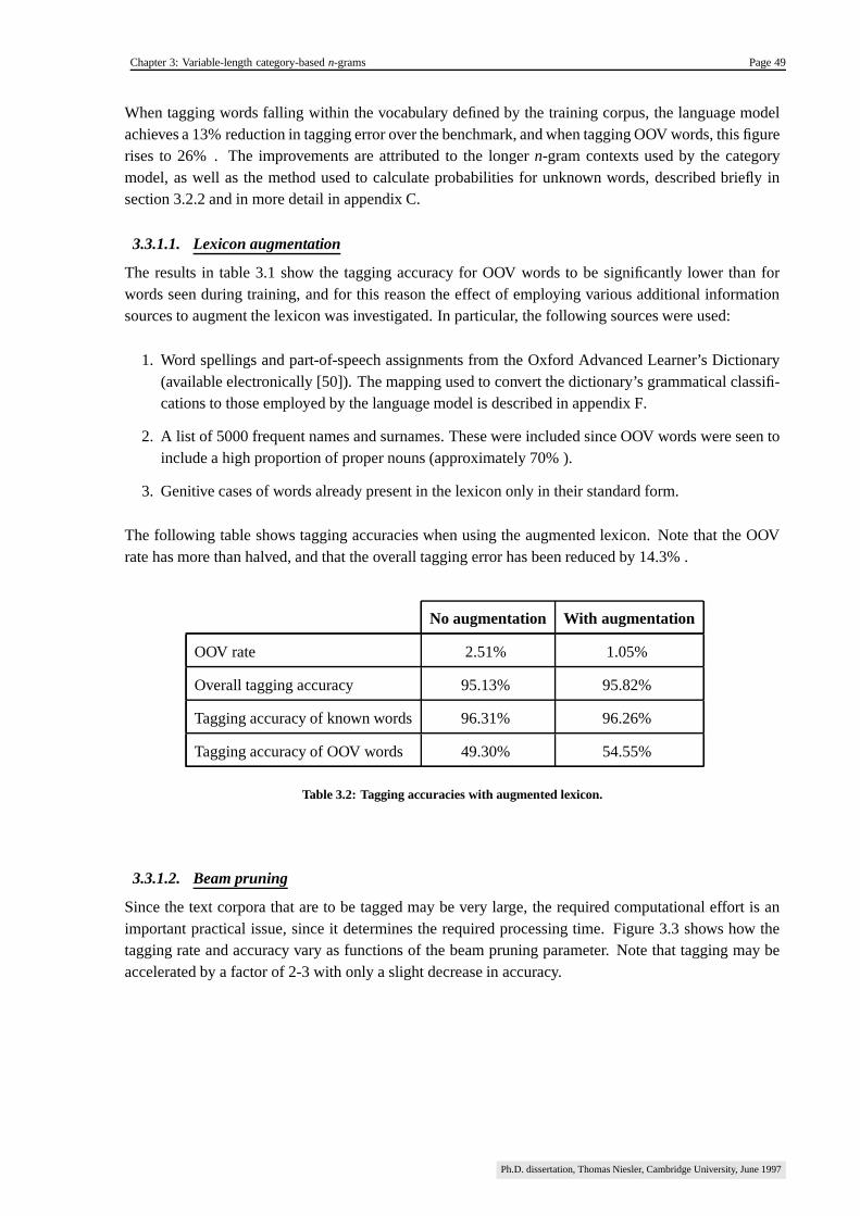
Chapter 3: Variable-length category-based n-grams Page 49
When tagging words falling within the vocabulary defined by the training corpus, the language modelachieves a 13% reduction in tagging error over the benchmark, and when tagging OOV words, this figurerises to 26% . The improvements are attributed to the longer n-gram contexts used by the categorymodel, as well as the method used to calculate probabilities for unknown words, described briefly insection 3.2.2 and in more detail in appendix C.
3.3.1.1. Lexicon augmentation
The results in table 3.1 show the tagging accuracy for OOV words to be significantly lower than forwords seen during training, and for this reason the effect of employing various additional informationsources to augment the lexicon was investigated. In particular, the following sources were used:
1. Word spellings and part-of-speech assignments from the Oxford Advanced Learner’s Dictionary(available electronically [50]). The mapping used to convert the dictionary’s grammatical classifi-cations to those employed by the language model is described in appendix F.
2. A list of 5000 frequent names and surnames. These were included since OOV words were seen toinclude a high proportion of proper nouns (approximately 70% ).
3. Genitive cases of words already present in the lexicon only in their standard form.
The following table shows tagging accuracies when using the augmented lexicon. Note that the OOVrate has more than halved, and that the overall tagging error has been reduced by 14.3% .
No augmentation With augmentation
OOV rate 2.51% 1.05%
Overall tagging accuracy 95.13% 95.82%
Tagging accuracy of known words 96.31% 96.26%
Tagging accuracy of OOV words 49.30% 54.55%
Table 3.2: Tagging accuracies with augmented lexicon.
3.3.1.2. Beam pruning
Since the text corpora that are to be tagged may be very large, the required computational effort is animportant practical issue, since it determines the required processing time. Figure 3.3 shows how thetagging rate and accuracy vary as functions of the beam pruning parameter. Note that tagging may beaccelerated by a factor of 2-3 with only a slight decrease in accuracy.
Ph.D. dissertation, Thomas Niesler, Cambridge University, June 1997

Chapter 3: Variable-length category-based n-grams Page 50
1 1.5 2 2.5 3 3.5 4 4.5 5 5.5 693
93.5
94
94.5
95
95.5
960 0.01
0.020.05
0.1
0.2
0.3
0.4
0.5
0.6
0.7
Normalised tagging rate
Ove
rall
tagg
ing
accu
racy
(%
)
Figure 3.3: Tagging rate and accuracy as a function of the beam pruning parameter.
3.3.1.3. Tagging the Switchboard and WSJ corpora
Since the Switchboard and Wall Street Journal (WSJ) corpora do not contain part-of-speech classifi-cations, they must be tagged before category-based models can be constructed. To accomplish this, alanguage model was built using the entire LOB corpus, after which its lexicon was augmented as in sec-tion 3.3.1.1. Finally, the most frequent OOV words in the respective corpora were determined, taggedby hand, and also added to the lexicon. Table 3.3 summarises this process.
Switchboard WSJ
Words in LOB corpus lexicon 42,258 42,258
Words added from dictionary 34,509 34,509
Additional proper nouns 5,037 5,037
Hand-tagged OOV words 452 1,888
Genitives 46,209 46,061
TOTAL 128,465 129,753
OOV-rate on training corpus 0.26% 1.19%
Table 3.3: Constitution of the augmented lexica for tagging Switchbaord and WSJ.
The category-based language model was used in conjunction with the corresponding augmented lexiconto produce tagged versions of both the Switchboard and the WSJ corpora.
Ph.D. dissertation, Thomas Niesler, Cambridge University, June 1997

Chapter 3: Variable-length category-based n-grams Page 51
3.3.2. Constructing category trees
Using the procedure detailed in section 3.2.1, category n-gram language model trees were constructedfor the LOB, Switchboard and WSJ corpora. The proposed tree pruning technique based on the leaving-one-out probability, termed likelihood pruning in the following, was evaluated by comparing it withtwo others: context-count pruning and n-gram-count pruning. The first discards all n-grams for whichthe
� � � � -gram context has been seen fewer than a threshold number of times. The second eliminatesall n-grams in the tree which have themselves been seen less often than a threshold, regarding them aspart of the unseen mass in probability calculations. Note that the latter approach is often used to makeword-based n-gram models more compact.
To illustrate the models obtained for different pruning thresholds, figure 3.4 graphs model size (totalnumber of n-grams in the tree) against the resulting category-perplexity (introduced at the end of section3.2.1) for the LOB corpus. Models obtained by n-gram-count pruning are not shown here since theirperplexities are off-scale, lying above 17.5.
0 0.5 1 1.5 2 2.5 3 3.5
x 105
13
13.5
14
14.5
15
15.5
Number of n−grams in tree
Cat
egor
y−pe
rple
xity 2e−04
1e−04
5e−05
1e−05
5e−062e−06
1e−065e−07
2e−07
1e−07
30
75
100
200
300
500
1000
Likelihood criterion
Context−count threshold
Figure 3.4: Model size versus performance for context-count and likelihood pruning on the LOB corpus.
From figure 3.4 we see that, as the complexity of the tree increases, the test set perplexity moves througha minimum. The initial decrease may be ascribed to underfitting of the data due to an insufficient numberof parameters, and the subsequent increase to overfitting of the data due to an excessive number ofparameters in the language model tree. Although its effect has been significantly reduced in comparisonwith context-count pruning, overfitting occurs despite the use of leaving-one-out cross-validation, whichremains an approximate way of modelling the test set. For all values of the pruning threshold, treesconstructed using likelihood-pruning exhibit a better size versus performance characteristic than thoseobtained by thresholding context counts. Similar behaviour has been seen for the Switchboard and WallStreet Journal corpora, except that in the last case the perplexity increase due to overfitting is smaller, aneffect which is ascribed to the larger amount of training material.
Ph.D. dissertation, Thomas Niesler, Cambridge University, June 1997

Chapter 3: Variable-length category-based n-grams Page 52
In order to determine how longer n-grams affect model performance, the category perplexity was mea-sured while limiting the maximum n-gram length in the tree to various values23. In particular, the treesobtained from the LOB training set by likelihood pruning (threshold
� � � � � � �� ), context-count prun-ing (threshold 200) and n-gram-count pruning (threshold 1) were used for these experiments, and theresults graphed in figure 3.5. We conclude that context-count pruning performs better than n-gram-countpruning24, although the difference is negligible for � ��� . This is due to the increasing sparseness ofn-grams and their contexts at higher � . In particular, individual n-grams occurring more often than thethreshold will cause n-gram-pruning to maintain a context which may deliver bad generalisation dueto a high proportion of unseen events in the test set. However, pruning based on the log probabilityoutperforms both approaches based on count thresholds.
1 2 3 4 5 6 7 8 912
14
16
18
20
22
24
26
28
Depth in tree (1 = unigram)
Cat
egor
y−pe
rple
xity
Likelihood−pruning
N−gram−count pruning
Context−count pruning
Figure 3.5: Evolution of the category-perplexity as a function of maximum n-gram length.
Consider now for each of the three corpora the tree obtained by likelihood pruning with� � � � � � �� .
Figure 3.6 analyses the proportion of n-grams in each model for each � , and from it we conclude that:
� For small � (unigrams and bigrams), the number of possible n-grams is small and so the numberof n-grams in the model is small.
� As � becomes large, the data become sparse, and consequently the cross-validated log probabilitypermits fewer n-grams to be added to the model.
� The WSJ corpus, which is much larger than the other two and therefore less sparse, has a largerproportion of n-grams with larger � .
23Although the results are not shown here, similar behaviour was observed for the word perplexity.24It may be possible to achieve better results by varying the threshold counts as a function of the n-gram length, but this was not investigated.
Ph.D. dissertation, Thomas Niesler, Cambridge University, June 1997

Chapter 3: Variable-length category-based n-grams Page 53
1 2 3 4 5 6 7 8 9 100
0.1
0.2
0.3
0.4
0.5
0.6
Length of n−gram (1 = unigram, 2 = bigram, etc.)
Fra
ctio
n of
tota
l n−
gram
s
LOB
SWBD
WSJ
Figure 3.6: Proportion of n-grams in the tree as a function of � .
Furthermore, when considering the evolution of the category-perplexities for each model with the addi-tion of each level to the tree, we find the behaviour illustrated in figure 3.7. Here each curve has beennormalised with respect to its bigram perplexity in order to facilitate the comparison. The greater size ofthe WSJ corpus allows longer n-grams to be of more benefit, and this is reflected by the larger relativedecreases in perplexity with the addition of 4-grams and higher. In contrast, the Switchboard corpus istoo sparse to merit the addition of 7-grams.
2 3 4 5 6 7 8 9 100.8
0.82
0.84
0.86
0.88
0.9
0.92
0.94
0.96
0.98
1
Length of n−gram (1 = unigram, 2 = bigram, etc.)
Nor
mal
ised
per
plex
ity
LOB
SWBD
WSJ
Figure 3.7: Perplexity as a function of maximum tree depth.
Ph.D. dissertation, Thomas Niesler, Cambridge University, June 1997

Chapter 3: Variable-length category-based n-grams Page 54
3.3.3. Word-perplexity
While the previous section has investigated the behaviour of the variable n-gram model using the cat-egory perplexity, here we consider the perplexities measured at the word level when implementing thelanguage model described in section 3.2. For all three corpora, category trees produced using a likeli-hood pruning threshold of
� � � � � � � in equation (78) are employed. The effect which limiting thenumber of maintained history postulates to �
����� � � has on performance is shown in the following table25.
Beam-pruning was not employed in this experiment.
Number of hypotheses ( ������ � � )
1 2 4 10 25
LOB 521.2 455.4 444.0 441.7 441.1
Switchboard 152.5 144.9 144.0 143.9 143.9
WSJ 522.7 483.2 477.1 476.2 475.8
Table 3.4: Perplexities when varying the maximum number of history postulates���������� .
The word perplexities decrease monotonically as the number of hypotheses is increased, demonstratingthat the history equivalence class ambiguity has a significant effect on the language model performance.The largest decrease occurs as �
����� � � is increased from 1 to 2, further increments leading to smaller
reductions. The figures in the table indicate that a value of approximately 10 will yield near-optimalresults, and therefore �
����� � � � ���
will be used henceforth. Having fixed ������ � � , it remains only to
decide on the value of the beam pruning parameter. Figure 3.8 shows its effect on perplexity for the LOBcorpus, and we conclude that a value less than
��� �"! should be chosen. Since a wider beam increasesthe computational effort, there is a tradeoff between the model accuracy and computational cost. Unlessotherwise specified, all experiments have been carried out with at value of
��� � � .
10−3
10−2
10−1
100
430
440
450
460
470
480
490
500
510
520
Beam−pruning threshold
Wor
d−pe
rple
xity
Figure 3.8: The effect of the beam pruning parameter on perplexity for the LOB corpus.
25For comparison, the perplexities of word-based n-gram language models for each corpus are given in appendix D
Ph.D. dissertation, Thomas Niesler, Cambridge University, June 1997

Chapter 3: Variable-length category-based n-grams Page 55
3.4. Comparing word- and category-based models
This chapter has introduced a language model based on variable-length part-of-speech n-grams. Word-based bigram and trigram models26 often remain the most successful and popular choice, however. Inview of this, the following sections present a detailed investigation into the relative performance of thesetwo approaches, in an attempt to determine the strengths and weaknesses of each [59]. All tests employlanguage models trained on the WSJ corpus, the category-based model having been produced with apruning threshold of
� � � � � � � as defined in equation (78).
3.4.1. Overall probability estimates
Firstly we investigate the differences in the values of the probability estimates delivered by each model.The histograms27 in figure 3.9 shows the number of words in the test set predicted with various logprobabilities by each model. Note in particular the following:
� The category-based model assigns probabilities less than��� � �
to a smaller proportion of words.
� A larger number of words is predicted with high probability (between 1.0 and 0.1) by the word-based than by the category-based model.
−10 −9 −8 −7 −6 −5 −4 −3 −2 −1 00
500
1000
1500
2000
2500
3000
3500
4000
4500
5000
Log probability
Num
ber
of e
stim
ates
Category−based model
Word−based model
Figure 3.9: Overall distribution of log probabilities produced by word- and category-based models.
We conclude that the ability of the category-model to generalise to unseen word sequences leads to thesmaller number of very low probabilities. However this same characteristic does not allow it to captureword-specific relations, and the strongest of these are responsible for the high-probability estimatesdelivered by the word-based model.
26As presented in section 2.4.27A bin size of 0.25 has been used.
Ph.D. dissertation, Thomas Niesler, Cambridge University, June 1997

Chapter 3: Variable-length category-based n-grams Page 56
3.4.2. The effect of backoffs
The objective here is to investigate the probability estimates made by the category-based model andthe word-based trigram when the latter does not back-off, or backs-off to various degrees. Table 3.5presents the perplexities calculated according to the type of word-model n-gram request and backoff.The category- and word-based models are denoted by “CBM” and “WBM” respectively.
Type of n-gram request % of test set CBM perplexity WBM perplexityUnigram 1.1 % 564.6 1,027.6Bigram (found) 19.3 % 321.6 95.3Bigram (backed-off to unigram) 2.3 % 15,110.3 73,541.4Trigram (found) 59.7 % 232.8 30.8Trigram (backed-off to bigram) 13.4 % 3,418.9 3,530.2Trigram (backed-off to unigram) 4.2 % 31,202.2 288,237.0
Table 3.5: Perplexities for various types of word n-gram requests.
From these results we may conclude that, when the word-based model does not back-off (a situationtrue for approximately 80% of the words in the test set), it performs significantly better on average thanthe category-based model. When backoffs do occur this is no longer true, and the intrinsic ability togeneralise to unseen word n-tuples allows the category-based model often to deliver better probabilityestimates. It is interesting to note that a significant proportion (approximately 22%) of the predictionsmade by the category-based model are as good or better than those of the word-model, even whenbacking-off does nor occur.
3.4.3. Per-category analysis
Here the objective is to analyse the contribution to the overall test set log probability made by individualcategories, as well as the average log probability associated with each, for non backed-off word n-grams.
The category is taken to be that assigned to the word by the same tagger used to tag the training cor-pus. Figures 3.10 and 3.11 illustrate28 the absolute fraction of the total log probability each category isaccountable for, while figure 3.12 shows the per-category average log probability. The horizontal axisindicates the frequency with which each such category occurs in the test set. From these figures weconclude that:
� As found in the previous section, when backing-off does not occur, the word-based model performsbetter than the category-based model.
� There is no clear relationship between the frequency of occurrence of a category and its perplexity,except that the categories with lowest average log probability also have been seen a very smallnumber of times (this is not visible in figure 3.12, but becomes evident on expansion of the hor-izontal axis by several orders of magnitude). These categories are sparsely trained as they havebeen seen only a small number of times in the training set.
28The following most significant grammatical categories have been labelled in these figures: common noun (NN), plural common noun(NNS), adjective (JJ), proper noun (NP), verb base form (VB), past tense of verb (VBD), past participle (VBN), present participle (VBG), third-person singular verb (VBZ), adverb (RB), preposition (IN), cardinal (CD), singular or plural article (ATI), singular article (AT), coordinatingconjunction (CC), subordinating conjunction (CS), letter of the alphabet (ZZ), end-of-sentence marker (SE), infinitival “to” (TO), unit ofmeasurement (NNU).
Ph.D. dissertation, Thomas Niesler, Cambridge University, June 1997

Chapter 3: Variable-length category-based n-grams Page 57
� Although some categories have low average log probabilities, they are infrequent and thereforemake a minor contribution overall.
� Common nouns (NN) are the most significant contributers to overall log probability, followed byplural common nouns (NNS), adjectives (JJ) and proper nouns (NP).
� In general it seems that words with semantic content, such as nouns and adjectives, are harder topredict (have lower probability) than syntactic function words (prepositions, articles, conjunctionsand personal pronouns). This is true for both word- and category-based models. The two verticallyseparated groupings in figure 3.12 illustrate this point.
� There appears to be an approximately linear relationship between the frequency with which acategory occurs and its contribution to the overall log probability. The constant of proportionalityis different for words with significant semantic content and syntactic function words respectively.This is emphasised by the two elongated groupings in figures 3.10 and 3.11.
0 0.02 0.04 0.06 0.08 0.1 0.12 0.14 0.16 0.18 0.20
0.02
0.04
0.06
0.08
0.1
0.12
0.14
0.16
0.18
0.2
Relative frequency of occurrence in test set
Fra
ctio
nal c
ontr
ibut
ion
to o
vera
ll lo
g pr
obab
ility NN
NNS
NP
CD
ATISE
ATZZ
VB
CC
JJ
RB
IN
functionSyntactic
categories
categoriesSemantic
VBDVBN
VBG
Figure 3.10: The contribution of each category to the overall test set log probability (word-based model).
Ph.D. dissertation, Thomas Niesler, Cambridge University, June 1997
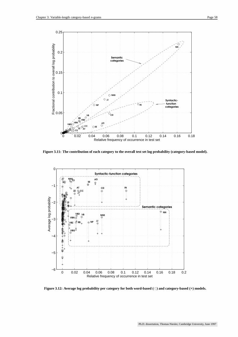
Chapter 3: Variable-length category-based n-grams Page 58
0 0.02 0.04 0.06 0.08 0.1 0.12 0.14 0.16 0.180
0.05
0.1
0.15
0.2
0.25
Relative frequency of occurrence in test set
Fra
ctio
nal c
ontr
ibut
ion
to o
vera
ll lo
g pr
obab
ility
IN
NNS
CD
SEAT
CC
CSZZ
RB
VBG
NP
JJ
categoriesfunctionSyntactic-
categoriesSemantic
VBN
VB
ATI
NN
VBD
Figure 3.11: The contribution of each category to the overall test set log probability (category-based model).
0 0.02 0.04 0.06 0.08 0.1 0.12 0.14 0.16 0.18 0.2−6
−5
−4
−3
−2
−1
0
Relative frequency of occurrence in test set
Ave
rage
log
prob
abili
ty
NN
ZZAT
SEATI
CD IN
Syntactic-function categories
VBD VB
TO
NNS
JJNPRB
VBG
NNU
CC
Semantic categories
VBZ
VBN
Figure 3.12: Average log probability per category for both word-based ( � ) and category-based (+) models.
Ph.D. dissertation, Thomas Niesler, Cambridge University, June 1997
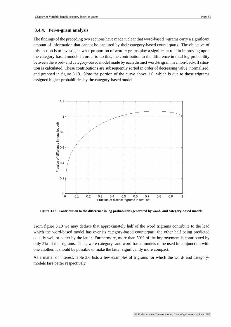
Chapter 3: Variable-length category-based n-grams Page 59
3.4.4. Per-n-gram analysis
The findings of the preceding two sections have made it clear that word-based n-grams carry a significantamount of information that cannot be captured by their category-based counterparts. The objective ofthis section is to investigate what proportion of word n-grams play a significant role in improving uponthe category-based model. In order to do this, the contribution to the difference in total log probabilitybetween the word- and category-based model made by each distinct word-trigram in a non-backoff situa-tion is calculated. These contributions are subsequently sorted in order of decreasing value, normalised,and graphed in figure 3.13. Note the portion of the curve above 1.0, which is due to those trigramsassigned higher probabilities by the category-based model.
0 0.1 0.2 0.3 0.4 0.5 0.6 0.7 0.8 0.9 10
0.2
0.4
0.6
0.8
1
1.2
Fraction of distinct trigrams in test−set
Fra
ctio
n of
diff
eren
ce in
tota
l log
pob
Figure 3.13: Contribution to the difference in log probabilities generated by word- and category-based models.
From figure 3.13 we may deduce that approximately half of the word trigrams contribute to the leadwhich the word-based model has over its category-based counterpart, the other half being predictedequally well or better by the latter. Furthermore, more than 50% of the improvement is contributed byonly 5% of the trigrams. Thus, were category- and word-based models to be used in conjunction withone another, it should be possible to make the latter significantly more compact.
As a matter of interest, table 3.6 lists a few examples of trigrams for which the word- and category-models fare better respectively.
Ph.D. dissertation, Thomas Niesler, Cambridge University, June 1997
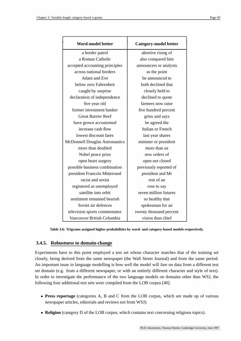
Chapter 3: Variable-length category-based n-grams Page 60
Word-model better Category-model better
a border patrol abortive rising of
a Roman Catholic also compared him
accepted accounting principles announcers or analysts
across national borders as the point
Adam and Eve be announced to
below zero Fahrenheit both declined that
caught by surprise closely held to
declaration of independence declined to quote
five year old farmers now raise
former investment banker five hundred percent
Great Barrier Reef grins and says
have grown accustomed he agreed the
increase cash flow Italian or French
lowest discount fares last year shares
McDonnell Douglas Astronautics minister or president
more than doubled more than us
Nobel peace prize new orders of
open heart surgery open not closed
possible business combination previously reported of
president Francois Mitterrand president and Mr
racist and sexist rest of an
registered as unemployed rose to say
satellite into orbit seven million futures
sentiment remained bearish so healthy that
Soviet air defences spokesman for an
television sports commentator twenty thousand percent
Vancouver British Columbia vision than chief
Table 3.6: Trigrams assigned higher probabilities by word- and category-based models respectively.
3.4.5. Robustness to domain-change
Experiments have to this point employed a test set whose character matches that of the training setclosely, being derived from the same newspaper (the Wall Street Journal) and from the same period.An important issue in language modelling is how well the model will fare on data from a different testset domain (e.g. from a different newspaper, or with an entirely different character and style of text).In order to investigate the performance of the two language models on domains other than WSJ, thefollowing four additional test sets were compiled from the LOB corpus [40].
� Press reportage (categories A, B and C from the LOB corpus, which are made up of variousnewspaper articles, editorials and reviews not from WSJ).
� Religion (category D of the LOB corpus, which contains text concerning religious topics).
Ph.D. dissertation, Thomas Niesler, Cambridge University, June 1997

Chapter 3: Variable-length category-based n-grams Page 61
� Scientific writing (category J of the LOB corpus).
� Fiction (categories K, L, N, P and R from the LOB corpus, consisting of adventure, mystery,Western, romantic and humorous fiction).
Table 3.7 summarises the performance of both the word- and category-based language models (WBMand CBM respectively) on these test sets. Performance on the WSJ test set is also shown for comparison.The category model used in this experiment was constructed with a pruning threshold of
� � � � � � �� .Test set No. of words % OOV Perplexity (WBM) Perplexity (CBM)WSJ baseline 56,820 0.67 144.4 450.5Press reportage 174,465 4.76 488.4 625.4Religion 33,215 5.52 549.4 598.0Scientific writing 154,755 6.63 624.3 671.7Fiction 239,927 6.13 643.0 715.0
Table 3.7: Performance of the category- and word-based models on different test sets.
Although the word-based model outperforms the category-based model in all cases, it is interesting tosee that, whereas the perplexity of the former increases by a factor of between 3.4 and 4.5, the perplexityof the latter does so only by a factor of between 1.3 and 1.6, indicating a reduced sensitivity to a changeof test domain.
3.5. Summary and conclusion
A category-based language model employing n-grams of varying lengths has been described. A proce-dure allowing n-gram length to be optimised with respect to estimated performance is presented, andexperiments using the LOB corpus show it to outperform conventional n-gram approaches while reduc-ing the number of model parameters. Words may belong to multiple categories, and consequently themodel bases its probability estimates on a set of possible classifications of the word history into categorysequences. Each such classification has an associated probability, and is updated recursively for eachsuccessive word in a sentence.
In order to capture syntactic patterns with this language model, the categories have been chosen to cor-respond to part-of-speech classifications. To make these classifications available for large but untaggedtext corpora, the application of the language model as a statistical tagger has been described, and exper-imental evaluation shows improved in tagging accuracy when compared with a benchmark.
The category-based language models are significantly more compact than word-based models, and offercompetitive performance in terms of perplexity, especially for sparse corpora. However, since categorymodels are never able to capture relationships between particular words, but only between the cate-gories to which these words belong, they are not able to fully exploit all the information available ina large training corpus. For this reason word-based models begin to perform significantly better as theamount of training material increases. However, closer analysis reveals that most of this lead is due toa relatively small proportion of n-grams in the word-model. In particular, category-based probabilityestimates remain competitive or superior in many instances, notably those for which the word-modelsneeds to back-off. For this reason category-based models display a greater robustness to changes in thecharacteristics of the testing domain.
Ph.D. dissertation, Thomas Niesler, Cambridge University, June 1997
Chapter 4: Word-to-category backoff models Page 62
Chapter 4
Word-to-category backoff models
4.1. Introduction
Section 3.4 has shown that the category-based language model presented in section 3.2 delivers betterprobability estimates in backoff situations due to its intrinsic ability to generalise to unseen word se-quences. It has also been shown that only a small fraction of word n-grams contribute to the largestpart of this difference in performance. In this chapter we consider a technique that allows backoffs totake place from a word- to a category-based n-gram probability estimate, with the aim of retaining theadvantages offered by each approach [58],[60].
4.2. Exact model
Consider the following language model, which backs off from a word- to a category-based probabilityestimate :
� � � � � ��� � � ��� � � � � � ��� � � if � � � � � � �� � � � �� � � � � ��� � � otherwise.
(89)
where :� � is the word for which we would like to estimate the probability of occurrence.
� � � is the word-history upon which the probability estimate of the word-based n-gram languagemodel depends, referred to the word-level context hereafter. For a bigram it is the preceding word,and for a trigram the preceding two words.
� � � is the word history and associated set of category history equivalence-class postulates uponwhich the probability estimate of the category-based model depends, termed the category-levelcontext hereafter. Due to the recursive nature in which the category history equivalence classpostulates are maintained29, the category-level context is in general only completely defined by theentire word history (i.e. to the beginning of the current sentence). Thus the number of category-level contexts is potentially huge, and the mapping from � � to � � is one-to-many.
� � � � � ��� � � is the probability estimate for � obtained from the word-based language model.
� � � � � ��� � � is the corresponding probability obtained from the category-based language model.
29Refer to section 3.2.3.
Ph.D. dissertation, Thomas Niesler, Cambridge University, June 1997

Chapter 4: Word-to-category backoff models Page 63
� � � � � � is the set of words in the word-context � � for which the word-model estimates will beused, backoffs occurring in other cases.
� ��� � is the backoff weight,��� � � � .
The estimate (89) is designed to employ word n-grams to capture significant sequential dependenciesbetween particular words, while using the category-based model for less frequent word combinations.From the requirement:
� � � � � � � � ��� � � � � � � � � � (90)
it follows from (89) that:
� � � � � �� � � 3
� � � ��� � � � � ��� � �� � � 3� � � � � � � � � ��� � � (91)
4.3. Approximate model
Due to the large number of different possible � � used by the category model, precalculation of� � �
according to equation (91) is not feasible. It would be more convenient to obtain backoff constantsfor every word-level context instead, but the dependence of the denominator of (91) upon � � does notpermit this, since it is not uniquely fixed by � � . Run-time calculation of
��� � using equation (91)increases the computational complexity of a probability calculation within any particular context by afactor of approximately
� in comparison with a model for which these parameters are precalculated,and thus represents a significant computational burden. To circumvent this, we note that the category-level context is most strongly influenced by the most recent words, and hence make the approximation:
� � � � ��� � � � � � � � � �� � � (92)
where�� � is the the category-level context corresponding to � � when assuming no prior knowledge of
the words preceding � � . Note that there is a unique�� � for each � � , so that we may define:
�� � � � ��� � � � ��� � �� � � �� � � for � � � �
� � (93)
and now we approximate the backoff weights by:
� � � � � � � ��� � �
�� � � � � � � for � � � �� �
and hence from (91) we find:
� � � � � �� � � 3
� � � � � � � � � ��� � �� � � 3� � � � � �� � � � ��� � � (94)
Ph.D. dissertation, Thomas Niesler, Cambridge University, June 1997

Chapter 4: Word-to-category backoff models Page 64
This choice of� � � in general no longer satisfies equation (90) however, and so we adjust the backoff
model (89) as follows:
� � � � � ��� � � ��� � � �� � � ��� � � if � � � � � � �� � � � �� � � � � ��� � � otherwise.
(95)
where� �� � � � � � � is some approximation of
� � � � � � � � . Now for equation (90) to be satisfied, itfollows from (95) that:
�� � � ��� � �� � � � � � � � � � �� � � � � � � � � � � �� �� � � � � � � � � ��� � � (96)
so we may choose to define:
� �� � � ��� � ����� � � � ��� � � � � ���� � � � � � ��� � � �� � � � � ��� � � (97)
where, in order to satisfy (96) we require that:
�� � � ��� � � � � � � � � � � � (98)
The quantity��� � � � � � � may be interpreted as a probability mass which must be distributed among
the elements of � by a suitable choice of � � � � � � � . The adopted approach is to distribute this mass
using the ratio:
� � � � ��� � �3� � � ��� � � � � ��� � � (99)
and therefore distribute probability mass to n-grams approximately in the same proportion as the word-based language model. Proceeding from equations (97) and (99), and employing the approximation (93)we are led to require :
� � � ��� � � � � �� � � � � � � � � � � �� �� � � � ��� � �� �� � � � � � � � � � � 3� � � � � �� � � � ��� � � � � � � � � � � �3
� � � � � � � � � ��� � �from which it follows that:
� � � � � � � �� � � � � � � � � � � � � �� � � � � �� � � � � � � �
�� � � � � � � � �3� � � � � � � � � � � � � � � � � �� �� � � � � � � � (100)
where
� � � ��� � � � � � � � � � � � � �� � � � � � (101)
Ph.D. dissertation, Thomas Niesler, Cambridge University, June 1997

Chapter 4: Word-to-category backoff models Page 65
This choice of � � � ��� � � satisfies equation (98). Furthermore, as:
�� � � � ��� � � � � � � � ��� � �we find from (94), (97) and (101) that:
� �� � � � � � � �
� �
� 3� � � ���� � � � � � � �� 3� � � � �� � � � � � � � �
� 3� � � ���� � � � � � � �� 3� � � ���� � � � � � � � �� � � ���� � � � � � � �
� ��
� � � � � � � � �3� � � � �� � � � � � � �
����
=
� �
�� 3
� � � � � � � � � � � � �� 3� � � ��� � � � � � � � �
� ��
� � �� � � � �� � � � � � � ���� �� � � � � � � � �3
� � � � � � � � � � � � �=� � � � � � � �
which means that the approximate backoff (95) converges to the exact backoff (89) as the estimates�� � � � ��� � � approach the exact values� � � � ��� � � .
Finally, although equation (100) guarantees:
� �� � � ��� � � � � (102)
when the approximation (92) is perfect, it does not do so in general. In order to guarantee (102) it issufficient to require:
� � � ��� � � � � (103)
so that, using equation (100) it follows that:
� � � � � � � � � � ��� � ��� � � � ��� � � � 3� � � � � � � � � ��� � � � � � � � � ��� � � � � 3
� � � � � �� � � � ��� � � � (104)
While calculating� � � � � , the equality in equation (104) should be enforced whenever the inequality
is violated. Referring back to equation (97), this is equivalent to demanding the probability mass dis-tributed to each word to be positive. In practice, this adjustment is required very infrequently.
The use of the estimates�� � � � allows the backoff constants � � � ��� � � and
��� � � � to be precalculated,making the model (95) significantly more computationally efficient than the exact model (89), whilecontinuing to employ in backoff situations the probabilities delivered by the category model.
Related research, carried out independently and concurrently, has recently been reported in [49]. Itdescribes a method that allows backoffs to occur from a word- to a category-based bigram language
Ph.D. dissertation, Thomas Niesler, Cambridge University, June 1997
Chapter 4: Word-to-category backoff models Page 66
model. In this case, however, words must belong to a unique category, which greatly simplifies thecalculation of the backoff weights.
4.4. Model complexity : determining� �
To this point it has been assumed that, for each word-level context � � , a set of words � has been
established for which probabilities will be calculated according to the word-based language model. Asimple choice for
� would be the set of all words seen within the context � � in the training set. Denotethis choice by � � , and note that when
� ��� � , backing-off occurs only for truly unseen events.
However, the approach taken here has been to reduce the size of � by eliminating words whose pres-
ence do not afford the word-based model much predictive power in relation to the category-based model.Since this process eliminates n-grams from the word-based model component, it allows the complex-ity30 of the word-to-category backoff language model to be reduced. Note that since the category-basedcomponent is fixed, it determines the minimum overall complexity.
The number of words in � has been reduced in two ways, both leading to similar results.
4.4.1. Testing n-gram counts
Consider a word � which has been seen in in context � � a total of �� � ��� � � times, and denote the
number of times the context � � itself was seen by � � � � � . Based on the category-model probabilityestimate
�� � � � ��� � � , the number of times we would expect to see � in � � is:
�� � � � ��� � � =
�� � � � ��� � �� � � � � �Assuming words to occur independently within each context, thus exhibiting a binomial distribution, thevariance of the count �
� � � � � � is [18]:
� � � � ��� � � =�� � � � ��� � �� � � �� � � � ��� � � � � � � � �
Using the normal approximation of the binomial distribution, we determine whether the actual count� � � ��� � � exceeds the expected count
�� � � � ��� � � by a certain fraction
�with a certain confidence �
by testing whether:
� � � ��� � � ��� � � �� �� � � � ��� � � � � � � � ��� � � (105)
where � is retained in � when the test succeeds. In practice the value of � is fixed (e.g. to 2.33 for 1%
or 1.645 for 5% confidence levels), and the value of�
is varied to control the size of � .
4.4.2. Testing the effect on the overall probability
Testing the n-gram counts as described in the previous section allows n-grams to be retained in � when
their counts are seen to differ from the expected ones in a statistically significant manner. The effect ofsuch pruning decisions upon the perplexity of the resulting language model is not clear, however. Moreprecisely, a frequent n-gram occurring only slightly more often in the word- than in the category-modelmight be discarded even though it has a significant effect on the overall probability due to its high
30The complexity of the word-to-category backoff model is taken to be the sum of the total number of n-grams in the word- and category-based components.
Ph.D. dissertation, Thomas Niesler, Cambridge University, June 1997

Chapter 4: Word-to-category backoff models Page 67
frequency. To avoid this, a second pruning criterion has been implemented, which discards those n-grams with the smallest effect on the training set log probability. The perplexity versus complexitytradeoff of the resulting models is similar to that achieved with the count-pruning method.
In particular, an n-gram is retained when:
� � � � (106)
where � �
is the change in mean per-word log probability when using the word-model instead of thecategory-model, and is calculated using:
� � � � � � ��� � �� � ������ � � � � ��� � � � ���� � �� � � � ��� � � � �� �
where � � is the total number of words in the training corpus 31.
4.5. Model building procedure
In summary of sections 4.3 and 4.4, the following steps need to be taken in order to construct a word-to-category backoff language model:
� Build a category-based language model as described in chapter 3.
� Build a word-based n-gram model.
� By application of equation (93), determine the probabilities�� � � � ��� � � for each n-gram in the
word model.
� For each context in the word-model, determine the set � using either equation (105) or equation
(106). This is essentially a process of pruning n-grams from the word model.
� For the remaining n-grams in the word-based model, calculate the � and�
values according toequations (100) and (94).
� Apply the language model according to equation (95).
4.6. Results
To gauge its performance, the backoff technique has been applied to the LOB, Switchboard and WSJtext corpora32. In each case language models of various complexities were generated by varying the sizeof
� as described in section 4.4, and the resulting perplexities compared with those achieved using aword trigram trained on the same data. The size of the latter was controlled by the standard techniqueof discarding n-grams occurring fewer than a threshold number of times in the training text (i.e. varyingthe n-gram cutoffs). Identical thresholds were employed for both bigrams and trigrams in all cases.
31Normalisation by the quantity���
makes� �
@and thus also � fairly corpus-independent.
32Descriptions of these corpora and their division into test- and training sets may be found in appendix D.
Ph.D. dissertation, Thomas Niesler, Cambridge University, June 1997
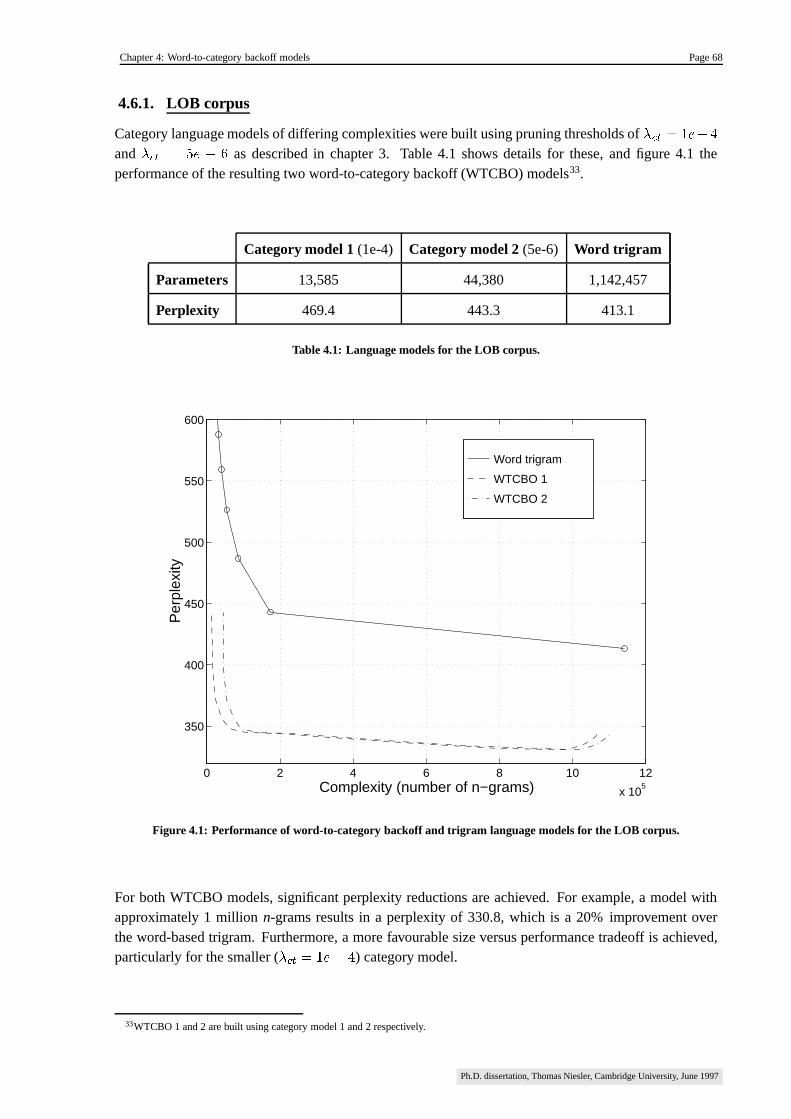
Chapter 4: Word-to-category backoff models Page 68
4.6.1. LOB corpus
Category language models of differing complexities were built using pruning thresholds of� � � � � � �
and� � � � � � � as described in chapter 3. Table 4.1 shows details for these, and figure 4.1 the
performance of the resulting two word-to-category backoff (WTCBO) models33.
Category model 1 (1e-4) Category model 2 (5e-6) Word trigram
Parameters 13,585 44,380 1,142,457
Perplexity 469.4 443.3 413.1
Table 4.1: Language models for the LOB corpus.
0 2 4 6 8 10 12
x 105
350
400
450
500
550
600
Complexity (number of n−grams)
Per
plex
ity
Word trigram
WTCBO 1
WTCBO 2
Figure 4.1: Performance of word-to-category backoff and trigram language models for the LOB corpus.
For both WTCBO models, significant perplexity reductions are achieved. For example, a model withapproximately 1 million n-grams results in a perplexity of 330.8, which is a 20% improvement overthe word-based trigram. Furthermore, a more favourable size versus performance tradeoff is achieved,particularly for the smaller (
������������ ) category model.
33WTCBO 1 and 2 are built using category model 1 and 2 respectively.
Ph.D. dissertation, Thomas Niesler, Cambridge University, June 1997

Chapter 4: Word-to-category backoff models Page 69
4.6.2. Switchboard corpus
Category-based language models were constructed again using pruning thresholds of� � � � � � � and
� � � � � � � , and table 4.2 shows the characteristics of these individual models while figure 4.2 showsthe performance of the resulting two word-to-category backoff (WTCBO) models.
Category model 1 (1e-4) Category model 2 (5e-6) Word trigram
Parameters 13,627 54,547 1,183,880
Perplexity 154.4 144.1 96.57
Table 4.2: Language models for the Switchboard corpus.
0 2 4 6 8 10 12
x 105
90
100
110
120
130
140
150
160
170
180
Complexity (number of n−grams)
Per
plex
ity
Word trigram
WTCBO 1
WTCBO 2
Figure 4.2: Performance of the word-to-category backoff and trigram models for the Switchboard corpus.
The larger category model leads to a word-to-category backoff model with lower minimum perplexityand improved performance for model complexities exceeding approximately 60,000 n-grams, while thesmaller leads to performance that is slightly diminished in this region but better for smaller numbers of n-grams. The word-to-category backoff model offers a slight improvement in perplexity with respect to thetrigram (approximately 2.7% in figure 4.2) and, depending on the choice of category model complexity,a significantly improved complexity versus performance tradeoff characteristic.
The limited number of conversational topics in the Switchboard corpus leads to a reduction in the trainingset sparseness and better coverage by the word trigram than for LOB (the trigram backoff rate drops by41% from the latter to the former). Thus there is less need for the generalising ability of the category-model, and consequently a smaller perplexity improvement.
Ph.D. dissertation, Thomas Niesler, Cambridge University, June 1997

Chapter 4: Word-to-category backoff models Page 70
4.6.3. WSJ corpus
For this corpus, results were determined only for one category-based model, which was constructedusing a pruning threshold of
� � � � � � � . Table 4.3 shows individual language model details, andfigure 4.3 the performance of the word-to-category backoff (WTCBO) and trigram models.
Category model Word trigram
Parameters 174,291 13,599,678
Perplexity 476.5 144.4
Table 4.3: Language models for the WSJ corpus.
0 2 4 6 8 10 12
x 106
100
150
200
250
300
350
400
450
500
Complexity (number of n−grams)
Per
plex
ity
Word trigram
WTCBO
Figure 4.3: Performance of word-to-category backoff and trigram language models for the WSJ corpus.
From figure 4.3 we see that, in this case, the word-to-category backoff model does not offer substantialperplexity improvements over the word-based trigram when the number of parameters is large. However,it nevertheless continues to offer a better complexity versus performance tradeoff. As was found for theSwitchboard corpus, perplexity improvements are small when the word-model is well-trained, which itis for WSJ due to the large quantity of training data.
4.7. Summary and conclusion
This chapter has presented a language model which backs-off from a word-based to a category-basedn-gram estimate. The category-model is able to generalise to unseen word sequences and therefore ap-propriate in backoff situations. When compared with standard trigram models, this technique greatlyimproves perplexities for sparse corpora, and offers significantly enhanced complexity versus perfor-mance tradeoffs.
Ph.D. dissertation, Thomas Niesler, Cambridge University, June 1997
Chapter 5: Word-pair dependencies in category-based language models Page 71
Chapter 5
Word-pair dependenciesin category-based language models
5.1. Introduction
An underlying assumption of the category-based language model presented in chapter 3 is that the prob-ability of a word depends only upon the category to which it belongs, and that its occurrence is thereforeequally likely at any point in a corpus where this category occurs. However, factors such as the topicand the style of the text may cause certain words to occur in groups, thereby violating this assumption.While short-term fixed-length word dependencies may be incorporated by means of word n-grams asdetailed in chapter 4, longer-term relations must be treated separately. This chapter presents a techniqueby means of which such long-range word associations may be captured by the category-based languagemodel. Explicit account is taken of the transient strength of the relationship as a function of a particulardefinition of the separating distance [61], [62].
Word-pairs have been combined with word n-gram language models within a maximum-entropy frame-work [79] [80], by linear interpolation [53], and as long-distance bigrams [93]. The development herediffers in that it takes explicit account of the distance between word occurrences, and takes specificadvantage of the category-based language model.
5.2. Terminology
Consider the effect which the occurrence of a trigger word-category pair� � � � ��� �� � � ��� � has on the sub-
sequent probability of occurrence of a target pair� � � � � � �� � � � � � . Refer to the sequence consisting of all
trigger occurrences as well as all words belonging to the target category as the trigger-target stream,and denote it by
� � � � � ��� �� � � � � � . Let the total number of words in the stream� � � � � ��� �� � � � � � be �
�,
and the number of occurrences of the trigger and target words respectively be �� � � � � ��� � and �
� � � � � � � � .It will henceforth be assumed that the stream has been taken from the training corpus, and under thiscondition we note that �
��� � � � ��� � � � � � � � � ��� �� � � ��� � and ���� � � � � � � � � � � � � � � � �� � � � � � where � � � � �� �
is the number of times in the corpus � occurs as a member of category�. Furthermore:
� � � �� � � � � � � � � if
� � � ��� � � � � � �� � � � � � � � � � � � � � � � ��� �� � � ��� � otherwise
where � � � � � is the number of times category�
occurs in the training corpus.
Ph.D. dissertation, Thomas Niesler, Cambridge University, June 1997

Chapter 5: Word-pair dependencies in category-based language models Page 72
Assuming the trigger and the target to be statistically independent, their occurrence probabilities within� � � � � ��� �� � � � � � are respectively given by:
� � � � � � ��� � � �� � � � � ��� �� � (107)
and� � � � � � � � � � � � � � � � � � �� � (108)
but since:
� � � � � � � � � � � � � � � � � � � � � � � �� � � � � �� � � � � � � � �
we see that the stream and category-conditional word probabilities for the target are related by:
� � � � � � � � � � � � � � � � � � � � � � � � � � (109)
with:
� � � � �� � � � � � � � � (110)
Define the separating distance � between a trigger-target pair as the number of times a word belongingto category
� � � � � is seen after witnessing the trigger and before the first sighting of the target itself.Hence � � � � � � � ������ ����
is the separating distance in the trigger-target stream. This definition ofdistance has been employed as a way of minimising syntactic effects on word co-occurrences, notably thephenomenon that there are certain categories which rarely follow one another for grammatical reasons.Syntactic effects should be reduced as much as possible since they are already modelled by the category� -gram component of the language model.
In the following a distinction will be drawn between the case where trigger and target are the same word(termed self-triggers) and the case where they differ (referred to as trigger-target pairs).
5.3. Probabilistic framework
Let the assumption that the probability of a word depends only upon its designated category, as stipu-lated by equation (52), be referred to as the independence assumption. Empirical investigation of thecategory-conditional probability � � � � � � � � as a function of the distance � reveals an exponential decaytowards a constant for words between which a correlation exists. Figure 5.1 illustrates this for the casewhere the trigger is the titular noun “president” and the target is the proper noun “congress”. 34
34The data are drawn from the WSJ corpus (refer to appendix D).
Ph.D. dissertation, Thomas Niesler, Cambridge University, June 1997
Chapter 5: Word-pair dependencies in category-based language models Page 73
0 10 20 30 40 50 60 70 80 90 1000
1
2
3
4
5
6
7x 10
−3
Distance (d)
Con
ditio
nal p
roba
bilit
y
Measured conditional probability
Independence assumption
Figure 5.1: Measured conditional probability ��������� � ����� of “congress” having seen “president”.
The transient behaviour displayed in this graph is typical, and has motivated the following postulatedform of the category-conditional probability:
� � � � � � � � � � � � � � � � � � ��� � � � � 1 � (111)
which is an exponential decay towards a constant probability� � in which � � and � define the strength
and rate of decay respectively. The stream-probability is found by scaling according to equation (109) :
� � � � � � � � � � � � � ��� � � � 1 � (112)
with� � � � � � � and � � � � � �� . Assuming the triggers to occur independently in the stream, their
probability� � is given by equation (107) :
� � = � � � � � � ��� � (113)
It follows that the probability mass function � � � � � for the target occurrence after sighting the trigger is:
� � � � � ���� � � �"!#� $'& � � � � � � � � � � 1 � � � � � � ��� � � � 1 � � (114)
The normalising constant � accounts for the probability mass associated with cases in which a triggerfollows another trigger before sighting the target.
The empirical estimates of figure 5.1 have been obtained by binning counts over the graphed distancerange. However, from a storage point of view, the potentially extremely large number of word-pairrelations make this approach infeasible for large-scale application, and hence it is not possible to obtainthe parameters of equation (112) from a direct fit to the data. The estimation of
� �, and then of � and � ,
is treated in the following two sections.
Ph.D. dissertation, Thomas Niesler, Cambridge University, June 1997

Chapter 5: Word-pair dependencies in category-based language models Page 74
5.3.1. Estimating���
The probability� �
may be estimated from the tail of the distribution, where the transient effect of theexponential term in (112) is assumed to be insignificant. Were the trigger and target to occur indepen-dently, their separating distance would have a geometric distribution, and we use its mean � �
as a roughindication of the point at which the exponential term becomes negligible:
� � � �� � � � � � � ��� � � � � � � � � � �� � � � � � ��� � � � ��� � � � � � � (115)
We could estimate� �
using counts of all trigger-pair occurrences with distances beyond this mean, i.e.:
� � � �� � � � � � � � � � ������ � � � ��� � (116)
where:
�� � � ����� =
�� � � � � � � � � � � ��� � if
� � � ��� � � � � � �� � � � � � � � � � � ����� � � � � � � � ��� �� � � ��� � � � ����� otherwise
and where � � � � � � � � � � � ����� , � � � � � � � � � � � ����� and � � � � � � ��� � � � ����� are the respective number of times thetarget word � � � � � , the target category
� � � � � , and the trigger word � � � ��� have been seen at distancesexceeding � �
in the trigger-target stream35. However, when �� � � � � � � � � � ����� is small, this estimate may
be unreliable, and therefore we introduce the following smoothed estimate:
� � ��� � ��� � � � � � � � � ��� ��� � � ����� � ��� � �� � � � � � � � � � (117)
with the parameter � chosen to be:
� � � ��� � � � � � � � � ������ ��� � � � � � � � � ��� � � �
Equation (117) is an interpolation of the relative frequency (116), and the relative frequency (108) ob-tained when pooling all the data (irrespective of � ). The interpolation weight � depends on the counts,and tends to unity36 as the number of sightings beyond � �
increases. The value of � is related to thenumber of sightings we consider to give us confidence in the estimate (116), since it determines howquickly � approaches 1. Hence it should be chosen to be a small constant greater than zero. All experi-ments were carried out with � � � � � , and its particular value was observed not to influence performancestrongly.
5.3.2. Estimating � and �Expressions allowing the determination of � and � from a knowledge of the mean and mean-squaredistances separating trigger and target have been derived. Since mean and mean-square calculationrequires little storage, this represents a memory-efficient alternative to a direct fit of the conditional
35In practice � was constrained always to exceed !&��
, and hence���
was clamped to a maximum of 3000 (3 time constants).36As � ! , equation (117) approaches equation (116).
Ph.D. dissertation, Thomas Niesler, Cambridge University, June 1997

Chapter 5: Word-pair dependencies in category-based language models Page 75
probability function (111) to measured binned data. In order to obtain closed-form expressions for themean and mean-square, the exact distribution was approximated by one of the form:
�� � � � � � ���� ! ��� � ! �� � ! ��� & ��� � & � � � & � (118)
where
� � � ! ��� & � � �(119)
The following equations relate the parameters of the exact and approximate distributions; details of theirderivation are shown in appendix G.
� � � ;��6 = ;�� � ;�� >�� 6 = ;� ;�� >(120)
� & � � � � � � (121)
� & � � � �� � � � � (122)
�! �
� � ��� � & � &� !
(123)
�! �
� ��� � & �� � � ����� � �� � � � � � � 6 � > ;������ � ��;���� � �(124)
The values of� � and
� �are calculated from the stream counts, using equations (113) and (117). In
order to solve for � & , � ! � and � , using the above equations, the measured mean � and mean-square � �distance between trigger and target is employed. However, when estimated from data, these quantitieshave been found to be sensitive to outliers. In particular, it may happen that the trigger and targetoccur in unrelated parts of the training corpus and are consequently separated by large quantities oftext37. Robustness is significantly improved by measuring the mean and mean-square within only apredetermined distance range, � � � � � � � � . Expressions for the mean-and mean-square expectedfor such truncated measurements38 under the independence assumption have been derived in appendixH. Since equation (118) is the superposition of two geometric terms, we may employ the results of thisappendix and express the truncated mean � � � � � and mean-square � � � � � � as a linear combination ofthe corresponding terms for truncated geometric distributions:
� � � � � ���� ���� ! ����! � � � ��� & � ��� & � � ��� (125)
and
� � � � � � ���� �� � ! �!���! � � � ��� & �! ��� & � � ��� (126)
Using equations (119), (120), (121), (122), (123), (124), (125) and (126), we may calculate � � � � � and� � � � � � given values for
� � , � � , � and � . Since it was not possible to solve explicitly for � and � interms of the other four parameters, however, their values were determined numerically by means ofnested bisection searches.
37This is a particular problem when information regarding the segmentation of the corpus, such as article boundary markers, is not available.38The geometric mean calculated using equation (115) was employed as a truncation interval in practice.
Ph.D. dissertation, Thomas Niesler, Cambridge University, June 1997
Chapter 5: Word-pair dependencies in category-based language models Page 76
5.3.3. Typical estimates
Figure 5.2 repeats the curves of figure 5.1, and adds the plot of equation (111) using the parameters� �
,� and � determined from the results of sections 5.3.1 and 5.3.2. The estimated conditional probabilityreflects the true nature of the data much more closely than that used under the independence assumption.
0 10 20 30 40 50 60 70 80 90 1000
1
2
3
4
5
6
7
x 10−3
Distance (d)
Con
ditio
nal p
roba
bilit
yMeasured conditional probability
Estimated conditional probability
Independence assumption
Figure 5.2: Measured and estimated conditional probability ����� � � � ��� of “congress” having seen “president”.
5.4. Determining trigger-target pairs
While the number of possible self-triggers is bounded by the vocabulary size, the number of potentialtrigger-target pairs equals the square of this number, and it is not possible to consider these relationsexhaustively except for very small vocabularies. In order to identify suitable candidates in a feasiblemanner, an approach employing two passes through the training corpus has been developed.
5.4.1. First-pass
This first stage of processing provides each potential target word in the lexicon with a tentative-list and afixed-list for trigger candidates. The latter contains words for which a reliable correlation with the targethas been established, while the former holds those for which no decision could yet be reached regardingthe presence or absence of such relationship. The tentative-list includes storage for the cumulative totalsrequired by distance-mean and -variance calculations, and is therefore more memory intensive than thefixed-list. At a certain point during processing, let the trigger-target pair have been seen �
�times at
separations� � & � ! ������� � � � �"! � , each falling within the chosen truncation interval � � , i.e.:
� � � � � � � � � � � ������ � � � �so that the measured mean is given by:
� � � � � � ���
� � �"!�� $'& � �Ph.D. dissertation, Thomas Niesler, Cambridge University, June 1997

Chapter 5: Word-pair dependencies in category-based language models Page 77
and the measured variance by:
� �� � � � � ��� *��
� ��"!�� $'& � � � � � � � � � �
Finally, assuming that the trigger and target occur independently, the expected mean is obtained fromthe truncated binomial distribution. Drawing on the results of appendix H we may therefore write:
� � � � � ��� � � � � -� � � ��� � � � � � � �"! � � � � *� �� ��� � � � � � � ���� � � � � ��� � � � � � � �where
� � � � � ��� � � � ��� � � � � � � � � � � � is the probability of occurrence of either trigger or target, calculateduniformly over the stream. Truncated mean- and variance-measurements are used to reduce the sensitiv-ity of the measurements to outliers. The statistics for members of the tentative list are updated on eachsighting the associated target during the sequential processing of the corpus. After each such updatetwo hypothesis tests, termed the kill- and fix-tests respectively, are used to decide upon the strength ofthe correlation. Since both the mean and the variance are measured from the data, and since empiricalobservation of the samples � � has indicated that they possess approximately normal distributions, thet-test [18] has been employed to make this decision in the following manner:
� The kill-test.
When the measured mean � � � � � is found to exceed the expected mean � � � � by a specified margin� � � � � and to a confidence of���, � � � � � � ��� ��� , the kill-test succeeds and the trigger candidate is
deleted from the tentative list. In particular, let:
� � � � � � � � � � ��� � � � � � � �The critical value � � of the mean is then:
� � � � � � � � � � � � � � � � � � �� � � � � ����
where��� � � � � � � � � � is the value obtained from the t-distribution for confidence
���' � � � � � � ��� ���and �
� *�degrees of freedom. The kill-test succeeds when � � � � � � � � , and figure 5.3 illustrates
these conditions.
t > µ killµKill because
µµ µµ
exp
kill t meas
Killmargin
Confidencemargin
µµ
kill
exp
margin
Don’t kill because
Kill
t µµ < kill
µµt meas
Confidencemargin
Figure 5.3: Illustration of the kill test.
Ph.D. dissertation, Thomas Niesler, Cambridge University, June 1997

Chapter 5: Word-pair dependencies in category-based language models Page 78
� The fix-test
When the expected mean � � � � is found to exceed the measured mean � � � � � by a specified margin� �� and to a confidence of
��� � �� � ��� ��� , the fix-test succeeds and the trigger candidate is
moved from the tentative- to the fixed-list. In particular, let:
� � � � � � � � ��� � � � �The critical value � � of the mean is then:
� � � � � � � � � � � � ��
� � � �� � � � � ����
where��� � �
�
� � � � is the value obtained from the t-distribution for confidence���" � �
� � ��� ���and �
� �degrees of freedom. The fix-test succeeds when � � � � � � , and figure 5.4 illustrates
these conditions.
µmeas µt µµexp
Fix because
fix
<µ fixt µ
Confidencemargin
Fixmargin
µ µmeas µ tµexp
fix
Fixmargin
Confidencemargin
µ µfixtDon’t fix because >
Figure 5.4: Illustration of the fix test.
The kill-test allows unpromising candidates to be pruned continually from the tentative list, therebycounteracting the explosion in the number of considered word-pairs that otherwise arises. Figure 5.5illustrates this by showing the growth in the number of tentative triggers when the kill-test is disabledand when it is active.
0 0.5 1 1.5 2 2.5 3 3.5 4
x 106
0
1
2
3
4
5
6
7
8
9
10x 10
6
Number of words processed
Num
ber
of te
ntat
ive
trig
gers
Kill−test disabled
Kill−test enabled
Figure 5.5: The effect of the kill-test on the total number of tentative triggers.
Ph.D. dissertation, Thomas Niesler, Cambridge University, June 1997
Chapter 5: Word-pair dependencies in category-based language models Page 79
Once a correlation has been established (and the fix-test succeeds), the trigger is moved from the ten-tative to the fixed list, and no further statistics need be gathered. Separate tentative- and fixed-listsare maintained since the latter can be made much more compact by not including storage for meansor variances. This is extremely important in view of the generally very large number of trigger-targetcandidates considered during the first pass.
Initially all tentative- and fixed-lists are empty. Furthermore, a record of the � most recent unique wordsis maintained during processing. As each word in the corpus is processed sequentially, each memberof this history is hypothesised as a possible trigger word, and for each such candidate the followingprocessing steps are performed:
� If this is not the first sighting of the target since the trigger, then END.� If the trigger is already in the fixed-list, then END.� If the trigger is not yet in the tentative-list, then:
– Add it to the tentative-list.
– Initialise the cumulative sum-of-distance and sum-of-squared-distance fields withthe first measurement.
– END.
� If the trigger is already in the tentative-list, then:
– Update the sum-of-distance and sum-of-squared-distance with the new measurement.
– Calculate the distance mean and variance.
– Calculate the expected mean under the independence assumption.
– Perform KILL and FIX t-tests :� Case A: The measured mean exceeds the independence-mean by a desired margin
and to a desired level of confidence; conclude that there is no correlation.� KILL: remove the trigger from the tentative list.� Case B: The measured mean is lower than the independence-mean by a desired
margin and to a desired level of confidence; conclude that there is a correlation.� FIX: remove the trigger from the tentative list and add it to the fixed-list.� Case C: neither of the above; conclude that there are as yet insufficient data to
reach a decision; do nothing.
– END.
The result of the first-pass is the set of all trigger-target relations present in the fixed-lists on completion,those remaining in the tentative-lists being discarded.
5.4.2. Second-pass
Since the fix-test in the first-pass uses means and variances often gathered only over a small portion ofthe training set, the detected correlations may be due to local anomalies which do not generalise to thecorpus as a whole. Consequently the second-pass recalculates the means and variances for all candidatesover the entire training corpus, and again applies the fix-test to each, discarding those which fail. Finally,the measured means and mean-squares of the remaining candidates are used to calculate the parameters� �
, � and � of the postulated conditional probability function.
Ph.D. dissertation, Thomas Niesler, Cambridge University, June 1997

Chapter 5: Word-pair dependencies in category-based language models Page 80
5.4.3. Regulating memory usage
Selection of the fix-test margin and confidence level allows the rate of transferrals from the tentative- tothe fixed-list to be regulated, and thus provides control over the growth and the final number of fixed-triggers. The kill-test parameters, on the other hand, affect the rate of deletions from the tentative-list.Finally, the length of the history � determines the rate of addition of new tentative trigger candidatesfor the current target.
The size of the tentative-list is of prime practical importance during first-pass processing, since eachentry requires significantly more storage than in the fixed-list. Despite the control over its size affordedby the choice of � and the kill-test parameters, it may still be difficult to limit the number of trigger-target pairs considered to practical levels. The following two refinements are employed as additionalmeasures in this regard.
1. Exclusion lists
Semantic correlations may be expected chiefly among content words, and since the grammaticalfunctions of words are known, it is possible to exclude non-content words from consideration astriggers or targets during processing. Practically this is achieved by means of an exclusion-listcontaining all grammatical categories that should be disregarded in this way.
2. Background culling
Observations during first-pass processing have shown a large number of tentative-list members tobe predominantly idle. These are infrequent trigger-target candidates which, once added to thelist, are neither fixed nor killed due to an insufficient number of measurements and long periodsbetween updates. In order to reduce the number of these cases, a process termed backgroundculling has been introduced. During processing, the distance to the last update is monitored formembers of the tentative list, and the decision boundary for the kill-threshold is moved graduallytowards that of the fix-threshold as this time increases. This relaxes the kill-test and ultimatelyforces a kill decision. The rate at which this occurs is normalised with respect to the frequency ofthe trigger, so that a single global parameter may be used to set the severeness of pruning.
Background culling is an approximation necessitated by practical considerations, and generallyintroduces errors by eliminating valid but infrequent trigger-target relations. However it allows thesize of the tentative list to be regulated to practical levels for large corpora and vocabularies, asillustrated in figure 5.6. Furthermore, the number of trigger-target pairs remaining after the second-pass appears in practice not to be affected strongly by the introduction of background culling. Inparticular, tests with the LOB corpus showed the number of tentative triggers after the first passto be reduced by 67 % , while the number of fixed-triggers surviving the second-pass fell by only3% . However, these figures depend on the fix- and kill-thresholds chosen during each pass.
5.4.4. Example pairs
Table 5.1 lists some examples of typical targets and their triggers found by the described technique whenapplied to the LOB corpus. The bracketed designations are the grammatical categories of the words inquestion39. It is appealing to find such intuitive relationships in meaning between word pairs gatheredaccording to purely statistical criteria.
39JJ = adjective, NN = common noun, NNS = plural common noun, NNU = unit of measurement, NP = proper noun,NR = singular adverbial noun, VB = verb base form, VBN = past participle.
Ph.D. dissertation, Thomas Niesler, Cambridge University, June 1997

Chapter 5: Word-pair dependencies in category-based language models Page 81
0 0.5 1 1.5 2 2.5 3 3.5 4
x 107
0
1
2
3
4
5
6
7x 10
6
Words of training set processed
Num
ber
of te
ntat
ive
trig
gers
Severe culling
Mild culling
No culling
Figure 5.6: The effect of background culling on the total number of tentative triggers.
Target Triggers
discharged (JJ) prison (NN), period (NN), supervision (NN), need (NN), prisoner (NN), volun-tary (JJ), assistance (NN)
advocate (NN) truth (NN), box (NN), defence (NN), honest (JJ), face (VB), case (NN), witness(NN), evidence (NN)
Cambridge (NP) university (NN), educational (JJ), affected (VBN), Oxbridge (NP), tomorrow(NR), universities (NNS)
worked (VBN) demand (NN), changes (NNS), cost (NN), strength (NN)
dry (JJ) currants (NNS), suet (NN), teasp. (NNU), wines (NNS), raisins (NNS)
judicial (JJ) legal (JJ), binding (JJ), rules (NNS)
semiindustrialised (JJ) world (NN), substantial (JJ), fall (NN), trade (NN), demand (NN), supply (NN)
cinema (NN) directors (NNS), viewing (NN), film (NN), festival (NN), tastes (NNS)
current (NN) inductance (NN), constant (NN), capacitor (NN), voltage (NN),
drowning (NN) respiration (NN), failure (NN), inhaled (VBN), body (NN), spasm (NN), sea(NN), salt (JJ), minutes (NNS), lethal (JJ), water (NN), resuscitation (NN), re-covery (NN), asphyxia (NN), survival (NN)
rotor (NN) r.p.m. (NNU), values (NNS), blade (NN), pitching (NN), speed (NN), flapping(NN), wind (NN), tunnel (NN), helicopter (NN), body (NN), rotors (NNS)
syntax (NN) language (NN), categories (NNS), formal (JJ), syntactic (JJ), grammatical (JJ),morphology (NN)
transfusion (NN) bleeding (NN), blood (NN), cells (NNS), ml (NNU), reaction (NN), haematoma(NN), transfusions (NNS), patient (NN), group (NN), treated (VBN)
increases (NNS) salary (NN), agreement (NN), salaries (NNS)
raisins (NNS) list (NN), lemon (NN), milk (NN), salt (NN), teasp. (NNU), brandy (NN),mixed (JJ), currants (NNS), suet (NN), sugar (NN), nutmeg (NN), oz (NNU),sultanas (NNS), eggs (NNS), peel (NN), apples (NNS)
Orpheus (NP) Heurodis (NP), Orfeo (NP), tale (NN), fairy (NN), Eurydice (NP)
Verwoerd (NP) policy (NN), Africa (NP), South (NP)
Table 5.1: Examples of triggers and targets collected from the LOB corpus.
Ph.D. dissertation, Thomas Niesler, Cambridge University, June 1997

Chapter 5: Word-pair dependencies in category-based language models Page 82
5.5. Perplexity results
The benefit of characterising trigger pairs as described in the previous sections was gauged by comparingthe performance of a category-based language model employing the independence assumption withanother using equation (111) but identical in all other respects. Experiments were carried out for theLOB and Wall-street Journal (WSJ) corpora40. Category-based language models were constructed foreach corpus using respective pruning thresholds of
� � � � � � � and� � � � � � � during construction of
the variable-length category n-grams. Word-pair distances were not calculated across article boundaries.
The details of the language models constructed for each of these corpora are summarised in table 5.2.Information for a standard trigram language model using the Katz backoff and Good-Turing discounting[41] is given in order to establish a baseline. The symbols � � , � � �
�and � � � � refer to the number
of words in the vocabulary, the number of n-grams in the trigram, and the number of n-grams in thecategory language model respectively. The number of self-triggers and trigger-target pairs for whichparameters were estimated41 are indicated by � � � and �
� �.
Corpus � � � � ��
� � � � � � � �� �
LOB 41,097 1,142,457 44,380 17,705 7,568
WSJ 65,000 13,047,678 934,894 49,952 83,696
Table 5.2: Language models and word-pair relations for the LOB and WSJ corpora.
Table 5.3 shows perplexities (PP) for the the trigram (TG) and category model (CM), and then for thecategory model with self-triggers (CM+ST), with trigger-target pairs (CM+TT), and lastly with bothself-triggers and trigger-target pairs (CM+ST+TT).
Corpus TG CMCM+ST CM+TT CM+ST+TT
PP % PP % PP %
LOB 413.1 443.3 369.2 15.6 439.9 0.8 368.9 16.8
WSJ 144.4 450.5 380.1 16.7 437.4 2.9 368.4 18.2
Table 5.3: Perplexities when including word-pair relations in the category-model.
Finally, the following table shows the perplexities (PP) obtained when the word-to-category backofflanguage models (WTCBO) developed in chapter 4 are used in conjunction with a category model em-ploying self-trigger and trigger-target pairs.
Corpus TGWTCBO WTCBO+ST WTCBO+ST+TT
Total n-grams PP PP PP Total%
LOB 413.1 138,678 368.9 291.1 291.0 29.5
WSJ 144.4 12,023,129 144.4 128.5 128.1 11.0
Table 5.4: Perplexities when including word-pair relations in the word-to-category backoff language model.
40Descriptions of the corpora many be found in appendix D.41Function words were excluded by means of a suitable exclusion list, as described in section 5.4.3.
Ph.D. dissertation, Thomas Niesler, Cambridge University, June 1997
Chapter 5: Word-pair dependencies in category-based language models Page 83
From table 5.4 we see that considerable reductions are obtained by combining the three approachesdescribed in chapters 3, 4 and 5 respectively. Note that, for the LOB corpus, the perplexity is reducedby almost 30% with respect to to the word-based trigram, while using only 12% as many parameters.
5.6. Discussion
The largest perplexity improvement is obtained for the WSJ corpus, for which the largest number ofself-trigger and trigger-target pairs were collected. This stems from the much greater corpus size andconsequent lower sparseness. For LOB on the other hand, many words occur too infrequently to makeestimation of the conditional probability parameters possible, thus leading to a reduced number of wordrelations.
For both corpora, the addition of self-triggers has a more significant impact on the perplexity than doesthe introduction of trigger-target pairs. This agrees with other reports in the literature [47], [53]. Self-triggers seem more reliable since the target, being its own trigger, is actually seen before being predictedto occur again. Trigger-target pairs, on the other hand, predict words that have either not yet been seen atall or have occurred in the distant past. Since such correlations are heavily dependent upon the topic ofthe passage, the effectiveness of a trigger-target association depends on how much the topics associatedwith a trigger coincide between the training- and test set. For the LOB corpus, which is very diverse inthe material it contains, there is a significant mismatch in this regard, leading to the observed very smallimpact of self-triggers on performance. For the WSJ corpus the mismatch is smaller, leading to greatersuccess.
Performance improvements obtained using the exponential decay self-trigger model (111) appears tocompare favourably with those obtained using a cache component, which has a similar philosophy, butusually does not allow the cache probability to decay with distance in a comparable way. In [45], forexample, the addition of a cache component decreases the perplexity of a part-of-speech language modelby 14% for the LOB corpus. In our experiments, the addition of self-triggers causes this figure to fallby 16.7% (table 5.3). For the WSJ corpus, perplexity improvements of between 14% and 17% havebeen achieved [24], [70], though these are harder to compare directly with our results since they includealso the effect of a bigram cache. Little information has been found in the literature regarding theperformance of language models incorporating trigger-target pairs. Experiments in [53] found that theiraddition by means of equation (64) improves only the perplexity of a unigram language model. Althoughsmall, the improvements shown in table 5.3 are nevertheless promising in this respect. The work reportedin [47] and [79] unfortunately does not show the individual impact on performance made by the cache,trigger-target pairs, or other added components. This is probably due to the numerically very intensivemaximum entropy technique used to combine these additional knowledge sources with the baselinetrigram language model. Finally, recent work affirms that also the performance of a standard cachecomponent may be enhanced by allowing the probabilities to decay exponentially [16].
The addition of self-triggers increases the number of parameters in the category-based model by � � � �(storage of � and � ). This increase is mild, and offers a favourable size versus performance tradeoff. Forinstance, the category model with self-triggers for LOB uses 62,085 parameters and achieves a lowerperplexity than the word-based trigram with 1.1 million parameters. Furthermore, the effectiveness ofboth types of word-pair modelling improves with corpus size, and since the parameter determinationand final implementation of the model has low memory requirements, the technique is suitable for usewith large training sets. This complements the category-based model, for which performance does notimprove in the same way.
Ph.D. dissertation, Thomas Niesler, Cambridge University, June 1997

Chapter 5: Word-pair dependencies in category-based language models Page 84
Finally, inspection of the values of � assigned to trigger-target pairs, as well as cases in which a triggersuccessfully predicts a target, shows that correlations well beyond the range of conventional n-grammodels are captured. Hence the proposed technique is indeed able to model long-range dependencies.This may also be deduced from the further reductions obtained when adding word-pair relations to thecategory-based model used within the word-to-category backoff framework (table 5.4). In particular,these improvements indicate that each of the three components contribute different information to themodel as a whole. The final 3-component models exhibit significantly lower perplexity than the baselineword trigram. This is true for both the LOB as well as the larger WSJ corpus, although the figure of29.5% for the former is particularly striking, and indicates that the imposition of the structure advocatedin section 1.3 is particularly effective when the training set is sparse.
5.7. Summary and conclusion
A new technique for modelling the empirically observed transient character of the occurrence probabil-ity between related words in a body of text has been introduced. Procedures both for the identification ofsuch word pairs as well as for the estimation of the three parameters required for the parametric modelhave been developed. Experiments demonstrate that meaningful relations are indeed identified, and thatthe transient behaviour (which often spans many words) is successfully captured by the proposed model.Perplexity reductions of between 16.8 and 18.2% were achieved, with the greatest improvement for thelargest and least-sparse corpus. Words correlated with themselves (self-triggers) had the most significantimpact on performance. The modelling technique is able to reduce the performance limit displayed bycategory-based models for large corpora, while maintaining their good performance versus size trade-off. Finally, when integrated into the word-to-category backoff framework, further improvements areachieved, allowing the baseline trigram language model perplexities to be surpassed. This reduction wasparticularly pronounced for the smaller LOB corpus, totalling 29.5% .
Ph.D. dissertation, Thomas Niesler, Cambridge University, June 1997

Chapter 6: Word error rate performance Page 85
Chapter 6
Word error rate performance
Perplexity is a popular measure of language model performance due to its lower computational demandswhen compared with a complete recognition experiment. However, reductions in perplexity do notguarantee reductions in recognition word error rates, which remain the ultimate measure of languagemodel quality. The following sections introduce methods by means of which language models may beincorporated into the recognition search, and finally present recognition results obtained for a Wall StreetJournal task using the language models developed in this thesis.
6.1. Language models in the recognition search
Ideally a connected speech recogniser should search the space of all possible concatenations of wordsto find the most likely combination with respect to the acoustic evidence. However, even for small vo-cabularies this exhaustive approach may be impractical, and thus more refined methods are necessary. Itis important from a practical standpoint to understand the mechanism of the decoding process, since thenature of the language model may heavily influence the complexity of the search problem. In particular,various alternative means of language model application are available, some of which are illustrated inthe remainder of this section. Consider as an example a speech recogniser which must recognise any3-word sentence containing the words “he”, “says” and “hello”. The set of possible sentences may bevisualised as the tree structure depicted in figure 6.1.
For connected speech the times at which word boundaries occur are not known. Since these affectthe probabilities obtained from the acoustic models by determining which segments of the observationsequence are assigned to which model, each possible choice of word-boundaries must be consideredto be a separate hypothesis by the recogniser. The total number of distinct hypotheses considered inthe search is therefore much larger than the number of sentences in the tree shown in figure 6.1, andhence it should come as no surprise that, even for small vocabularies, the search space is in practice toolarge to be considered exhaustively. The size of the search space is limited by practical constraints suchas processing time and available storage, and hence the following two techniques are instrumental inmaking recognition practical [66].
1. Path-pruning : As the search proceeds, certain hypotheses will become very unlikely, and maybe discarded to save computation and storage. However, since it cannot be guaranteed that one ofthese paths is indeed the correct result (becoming much more probable later on), pruning may leadto search errors.
Ph.D. dissertation, Thomas Niesler, Cambridge University, June 1997
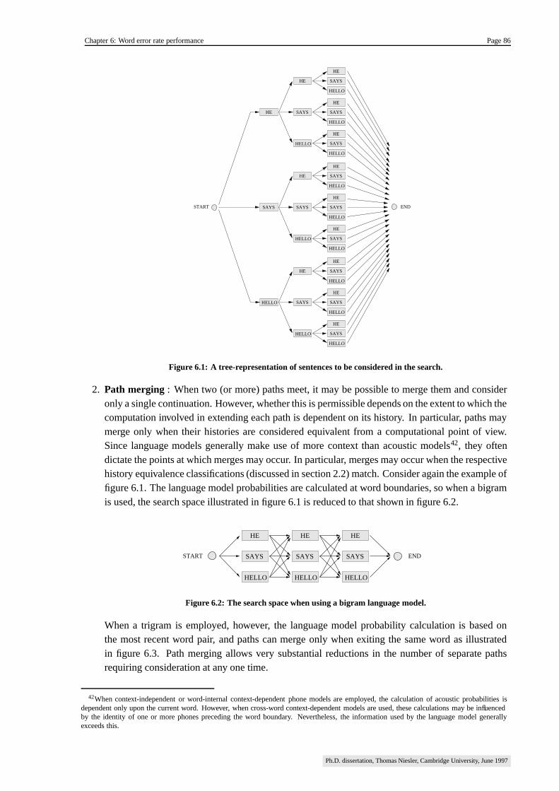
Chapter 6: Word error rate performance Page 86
SAYS
HE
HE
HELLO
SAYS
HELLO
SAYS
HELLO
HELLO
HE
HE
SAYS
SAYS
HELLO
HELLO
HE
HE SAYS
SAYS
HELLO
HELLO
HE
HE
HE
SAYS
SAYS
HELLO
HELLO
HE
HELLO
SAYS
HE
HELLO
SAYS
HE
HE
SAYS
SAYS
HELLO
START END
Figure 6.1: A tree-representation of sentences to be considered in the search.
2. Path merging : When two (or more) paths meet, it may be possible to merge them and consideronly a single continuation. However, whether this is permissible depends on the extent to which thecomputation involved in extending each path is dependent on its history. In particular, paths maymerge only when their histories are considered equivalent from a computational point of view.Since language models generally make use of more context than acoustic models42, they oftendictate the points at which merges may occur. In particular, merges may occur when the respectivehistory equivalence classifications (discussed in section 2.2) match. Consider again the example offigure 6.1. The language model probabilities are calculated at word boundaries, so when a bigramis used, the search space illustrated in figure 6.1 is reduced to that shown in figure 6.2.
HELLO
SAYS
HE
SAYS
HE
SAYS
HE
HELLO HELLO
START END
Figure 6.2: The search space when using a bigram language model.
When a trigram is employed, however, the language model probability calculation is based onthe most recent word pair, and paths can merge only when exiting the same word as illustratedin figure 6.3. Path merging allows very substantial reductions in the number of separate pathsrequiring consideration at any one time.
42When context-independent or word-internal context-dependent phone models are employed, the calculation of acoustic probabilities isdependent only upon the current word. However, when cross-word context-dependent models are used, these calculations may be influencedby the identity of one or more phones preceding the word boundary. Nevertheless, the information used by the language model generallyexceeds this.
Ph.D. dissertation, Thomas Niesler, Cambridge University, June 1997

Chapter 6: Word error rate performance Page 87
HE
SAYS
HELLO
HELLO
HELLO
SAYS
HE
SAYS
HELLO
HE
HE
HELLO
SAYS
SAYS
SAYS
HE
HELLO
HELLO
HE
HE
SAYS
START END
Figure 6.3: The search space when using a trigram language model.
For trigram and longer-span language models, the number of paths may become unmanageably largeeven with efficient path merging. Containing the search would require more severe pruning, whichmight unacceptably increase the number of search errors. In such cases we may adopt the followingtwo-pass strategy:
1. Apply a simpler (e.g. bigram) language model during the recognition search, and output a sub-set of the search space containing a number of the most likely paths, termed the intermediatehypotheses.
2. Post-process, or rescore, the intermediate hypotheses by applying the more sophisticated languagemodel, and pick the most likely as the final recognition result.
As long as the result that would be obtained after a recognition search using the more sophisticated lan-guage model is among the intermediate hypotheses, the final result will remain unaffected by the divisionof the recognition process into two stages. However, when the first-pass eliminates this hypothesis, asearch error occurs which the second-pass is unable to correct. The accuracy43 of the intermediatehypotheses is affected both by the exactness of the first pass as well as the size44 of the intermediatehypotheses, and is an important issue when taking the two-pass approach.
Two forms of intermediate hypotheses, N-best lists and lattices, are described in the following sections.
6.1.1. N-best rescoring.
The N-best method [82] determines during the recognition search a list containing the � most likelyhypotheses, together with the acoustic and language model probabilities for each word. The new lan-guage model is used either to replace or to modify the existing probabilities for each hypothesis, afterwhich the overall likelihood is recalculated. The recognition result is the highest ranking hypothesis inthis new list.
43The proportion containing the result of a full recognition search.44The number of alternatives.
Ph.D. dissertation, Thomas Niesler, Cambridge University, June 1997

Chapter 6: Word error rate performance Page 88
6.1.2. Lattice rescoring.
Instead of a list, the recognition search may output a network containing the most likely paths in therecognition search space. A lattice is a directed acyclical graph in which the nodes correspond toword boundaries in time, and the links between the nodes correspond to particular word hypotheses.Acoustic and language model likelihoods for each word are stored in the lattice, and each path from thestart to the end node represents a distinct hypothesis. The most likely path through the lattice may befound using a suitable search algorithm, A* having been applied successfully [66], [67]. A lattice is amuch more compact representation of a set of alternatives than an N-best list, and in certain situationsthe lattice search may be performed very efficiently. However, a prerequisite is that significant pathrecombination is possible, else the number of separate paths maintained during the lattice search maybecome unmanageable. For N-best lists on the other hand, the storage and computational effort requiredduring rescoring is well defined a-priori. Note that N-best lists may be generated from lattices.
6.2. Recognition experiments
This section presents recognition results in terms or word error rates obtained using the language modelsdeveloped in this thesis. The experiments were conducted on the WSJ corpus by using lattices gener-ated at Cambridge University with the HTK large-vocabulary speech recognition system as part of theNovember 1994 ARPA CSR evaluation [91]. The HTK recogniser uses mixture Gaussian cross-wordcontext dependent hidden Markov acoustic models and allows scoring in a single pass, while incorporat-ing an n-gram language model to deliver state-of-the art performance. Lattices produced for the 65,000word vocabulary 1994 H1 development test were rescored using the baseline bigram and trigram lan-guage models described in appendix D. The resulting trigram lattices were used to generate N-best lists,which were subsequently rescored by the new language models to obtain the final recognition results, asdescribed in section 6.1.1. The following section presents the baseline recognition performance, whileensuing sections show how this performance changes on application of the various language models.Language model scaling factors used in the rescoring were optimised approximately for the test set inall cases, including the baseline.
6.2.1. Baseline results
There are 310 lattices in the development test set, comprising approximately 15 sentences from each of20 speakers, and leading to a total of 7,388 words in the reference transcription. The out-of-vocabularyrate of the 65,366 word vocabulary, with respect to the reference transcription, is 0.28% . Since theoriginal lattices were constructed using a language model trained on substantially more data than WSJ87-89, they were rescored using the bigram and trigram language models described in appendix D toobtain baseline recognition accuracies, and these are shown in the following table. Perplexities areshown both for the language model (LM) test set (appendix D), as well as the H1 development testreference transcription.
Perplexity% Word error
LM test set H1 dev-test ref.
Baseline bigram 215.4 275.6 13.66
Baseline trigram 144.4 204.3 11.84
Table 6.1: Baseline performance for the 1994 H1 development test set.
Ph.D. dissertation, Thomas Niesler, Cambridge University, June 1997
Chapter 6: Word error rate performance Page 89
Changes in system performance after application of the language models will be measured relative tothe baseline trigram error rate of 11.84% . To obtain an indication of the best possible recognitionperformance obtainable with the lattices and N-best lists, the error rate for each is shown in table 6.2.
Error rate
Lattices 1.57 %
N-best (N=100) 5.36 %
Table 6.2: Lower bounds on word error rates.
Since all recognition experiments in the following sections will rescore the 100 best hypotheses of eachof the lattices, the lowest achievable word error rate is 5.36% .
6.2.2. Rescoring results
The Entropic Lattice and Language Modelling Toolkit [67] was employed as an interface allowing con-venient N-best rescoring with the new language models. In particular, the tools were used to determinethe 100 best hypotheses from each lattice, to rescore these using the new language models, to re-rank theresult, and finally to output the best hypothesis in the rescored list. The new language models were eitherused to replace the baseline language model probabilities entirely, or were combined with the baselinetrigram by linear interpolation. Various combinations of the language model components presented inthis thesis were used in the rescoring process, and results for each are shown in the following sections.
6.2.2.1. Category model
The variable-length category-based n-gram model developed in chapter 3 and constructed with pruningthreshold
� � � � � � � was used to rescore the N-best lists by means of linear interpolation with thebaseline trigram probabilities, which are already present in the lattice. The following table summarisesthe results obtained for various interpolation conditions, perplexities again being shown for both the testset described in appendix D as well as the reference transcription. The interpolation parameter weightsthe category-model, and thus a value of zero corresponds to rescoring using the baseline trigram only.
WeightPerplexity
% Word error % Improvement
LM test set H1 dev-test ref.
0.0 144.4 204.3 11.84 -
0.15 134.6 183.2 11.64 1.7
0.25 135.4 181.7 11.45 3.3
0.5 147.5 192.3 11.44 3.4
0.75 180.4 228.1 11.76 0.7
1.0 450.5 508.6 12.49 -5.5
Table 6.3: Rescoring using the category-based model interpolated with the baseline trigram.
Interpolation is able to reduce the perplexity of the baseline trigram by approximately 7 % on the test
Ph.D. dissertation, Thomas Niesler, Cambridge University, June 1997
Chapter 6: Word error rate performance Page 90
set and 11 % on the reference transcription, while resulting in a 3.4% improvement in the error rate.Note however that optimum performance is not achieved at the lowest perplexity on the test set. Similarobservations have been made in [21] and [80]. Performance appears to be relatively insensitive to theinterpolation weight while this is in the range 0.25 to 0.5.
6.2.2.2. Word-to-category backoff model
The word-to-category backoff models developed in chapter 4 were used to rescore the N-best lists by re-placing the lattice scores entirely. The category model constructed with a pruning threshold of � �
�was
used, and experiments were carried out for word-to-category backoff models of different complexities,as shown in the following table.
Number of n-grams Perplexity % Word error % Improvement
LM test set H1 dev-test ref.
12.0M 144.4 197.8 11.52 2.7
11.6M 144.8 198.2 11.53 2.6
6.7M 151.3 204.5 11.69 1.3
1.0M 238.0 298.5 12.09 -2.1
Table 6.4: Rescoring using only the word-to-category language model.
These results show a word error rate improvement of 2.6% for the most complex model (which retainsmost of the word model’s n-grams), but smaller improvements and eventual deterioration in performancewhen the number of parameters is reduced. Better performance both in terms of perplexity and worderror rate is achieved by linear interpolation with the baseline, as was shown in table 6.3.
6.2.2.3. Category model with long-range correlations
Since the word-pair relations described in chapter 5 require the determination of their separating dis-tance, a record must be kept of the document history. This is achieved by retaining the best recognitionoutput for each lattice to the beginning of the current article, while processing the lattices in the orderthey were spoken. The following table shows perplexities and recognition results obtained when incor-porating first self-triggers (ST) and then also trigger-target (TT) pairs into the category model used insection 6.2.2.1. Linear interpolation with a weight of 0.5 was employed in the rescoring process.
Configuration Perplexity % Word error % Improvement
LM test set H1 dev-test ref.
Category + ST 127.3 161.8 11.22 5.2
Category + ST + TT 126.7 160.8 11.18 5.6
Table 6.5: The category-based model with word-pair correlations interpolated with the baseline trigram.
The linear interpolation of the category-based model including word-pair relations has decreased theperplexities with respect to the baseline by 12.3 % and 21.3 % on the test set and reference transcriptionrespectively, and has led to a word error rate improvement of 5.6% . This improvement has been verified
Ph.D. dissertation, Thomas Niesler, Cambridge University, June 1997

Chapter 6: Word error rate performance Page 91
to be significant at the 5% level45 using a NIST scoring package [63]. As is the case for the perplexity,the largest part of the reduction in word error rate has been brought about by the addition of self-triggers.
6.2.2.4. Word-to-category backoff model with long-range correlations
Finally, the word-to-category backoff (WTCBO) model with 12.0 million parameters was used to rescorethe N-best lists as in section 6.2.2.2, however now employing the category-based model with word-pair relations evaluated on its own in the previous section. Perplexities and recognition results whenincluding both self-triggers (ST) and trigger-target (TT) pairs are shown in the following table.
Configuration Perplexity % Word error % Improvement
LM test set H1 dev-test ref.
WTCBO + ST + TT 128.1 167.5 11.59 2.1
Table 6.6: Rescoring using the word-to-category backoff model with word-pair correlations.
Although the perplexities are similar to those reported in table 6.5, improvements in the word error rateare smaller. Furthermore, it is disappointing to note that the addition of the word-pair relations has ledto a deterioration of the word-to-category backoff model, results for which were shown in table 6.4.
6.3. Summary and conclusion
The use of the category-based language model in the N-best rescoring framework has led to improve-ments in recognition word error rate, when applied either by linear interpolation with the lattice-internaltrigram probabilities or by means of the word-to-category backoff method. Subsequent addition of long-distance word correlation models lead to further improvements when interpolating the category modelwith the baseline trigram, but not in conjunction with the word-to-category backoff method. Since thebaseline trigram language model probabilities are already present in the lattice, linear interpolation isboth simpler to implement and less memory intensive, and should therefore be the method of choice forsimilar recognition problems. Interpolation with the category-based model employing both self-triggersand trigger-target pairs led to a relative word error rate improvement of 5.6% over the baseline, and thisfigure has been verified to be statistically significant.
45There is a less than 5% probability that the improvement is by chance.
Ph.D. dissertation, Thomas Niesler, Cambridge University, June 1997

Chapter 7: Summary and conclusions Page 92
Chapter 7
Summary and conclusions
This thesis has focussed on the use of linguistically-defined word categories as a means of improvingthe performance of statistical language models. In particular, an approach that aims to capture bothgeneral grammatical patterns as well as particular word dependencies by different model componentswas developed and evaluated.
7.1. Review of conducted work
The separate treatment of patterns due to syntax and patterns due to semantic relationships has led tothree distinct sections in this document. The first section, in chapter 3, develops a model for syntacticdependencies based on word-category n-grams. The second section, in chapter 4, extends this model byallowing short-range word relations to be captured through the incorporation of selected word n-grams.Finally, a technique which permits also the inclusion of long-range word-pair relationships is presentedin chapter 5.
7.1.1. The category-based syntactic model
The n-gram has proved a very successful model for short-term word dependencies. Noting that Englishgrammatical constructs are often quite local in nature, n-grams of part-of-speech word-categories wereadopted as a means of capturing general sequential grammatical patterns.
Since there are significantly fewer parts-of-speech than there are words in a typical vocabulary, thesemodels contain a much smaller number of n-grams than a comparable word-based model. This reducesthe sparseness of the data with respect to the number of parameters, which in turn allows us to capturelonger-range effects by increasing � . Furthermore, an important advantage of category n-grams is theirintrinsic ability to generalise to word n-tuples not seen during training. Part-of-speech categories embedsyntactic information, and hence this generalisation proceeds according to the measure of grammaticalcorrectness assigned to the unseen sequence by the model.
Chapter 3 proposes, develops, and evaluates a model employing category-based n-grams of variablelength. Each word may belong to more than one category in order to account for different grammaticalfunctions. The length of individual n-grams is optimised by allowing it to increase as long as furtherextension benefits the overall predictive quality. In order to avoid overfitting of the training set, the cri-terion used to estimate this predictive quality is based on leaving-one-out cross validation. The languagemodels produced in this way are seen to contain n-grams whose length varies between one (unigram)and a maximum of four to fifteen, depending on the nature and amount of training material, as well asthe parameters used during model construction.
Ph.D. dissertation, Thomas Niesler, Cambridge University, June 1997

Chapter 7: Summary and conclusions Page 93
Words may belong to several part-of-speech categories to account for multiple grammatical functions.Therefore, when calculating the probability of a particular word in a sentence based on the words seenbefore, the language model must take into account the many possible category sequences that correspondto this word history. An algorithm by means of which this may be achieved for the variable-lengthcategory-based model was developed in chapter 3. This algorithm consists of a recursive procedurethat maintains a set of possible category sequences for the word history, with an associated probabilityfor each. These probabilities have been employed also in assigning category classifications to new text,hence configuring the language model as a tagger. In this way 1.9 million words of transcribed telephoneconversations and 37 million words of Wall Street Journal text were assigned part-of-speech tags, thusmaking it possible for category-based language models to be trained on both corpora.
Experimental evaluation has shown that, when used as a tagger, the variable-length category-based lan-guage model is able to deliver better results than a baseline system. Particularly significant improve-ments were achieved when tagging out-of-vocabulary words as a result of the proposed method forcategory-membership probability estimation based on cross validation. The algorithm developed to se-lectively extend the length of individual n-grams has led to better results than achieved by commonlyused pruning methods based on count thresholds. Consequently, the variable-length models outperformconventional fixed-length approaches. Language model perplexities are seen to be competitive for sparsetraining sets, but not for larger ones, although large reductions in the number of model parameters arefound in all cases. When interpolated with a word-based trigram, the category-based model has led toa 3.4% word error rate improvement for a Wall Street Journal recognition experiment within an N-bestrescoring framework.
7.1.2. Inclusion of word n-grams
A language model based purely on category n-grams is not able to capture relationships between particu-lar words, but only between the categories to which these words belong. In chapter 3, a detailed compar-ison between a conventional trigram and the variable-length category-based language model has shownthat the former gives better estimates for word n-grams seen in the training set, but not in other cases.Word n-grams are an effective means of encoding short-term relationships between particular words,while category n-grams generalise to unseen word sequences and are therefore particularly appropriatein backoff situations. Chapter 4 develops a technique that allows a word-based n-gram language modelto back-off to the category-based model presented in chapter 3, thereby combining the strengths of bothapproaches. An exact formulation would require an excessive number of backoff weights, due to thecomplex representation of the word history used by the category model in its probability calculations.Hence, an approximate model is developed which continues to employ the category model in backoffsituations, and ensures correct normalisation by approximating the word-model probabilities. Further-more, a procedure is proposed which selects only the most important word n-grams for inclusion intothe word model, thus allowing the overall number of parameters to be traded for modelling accuracy.Experiments show these methods to deliver greatly reduced perplexities for sparse training sets, andsignificantly improved size versus performance tradeoffs when compared with standard trigram models,even for large corpora. Recognition experiments performed within an N-best rescoring framework showthat the proposed technique fares approximately as well as a linear interpolation of the category-basedmodel with the baseline trigram.
Ph.D. dissertation, Thomas Niesler, Cambridge University, June 1997

Chapter 7: Summary and conclusions Page 94
7.1.3. Inclusion of long-range word-pair relations
An underlying assumption of the category-based model is that the probability of a word depends onlyupon the category to which it belongs, and that its occurrence is therefore equally likely at any pointin a corpus at which this category occurs. However, factors such as the topic and the style of the textcause certain words to occur in groups, thereby violating this assumption. While the inclusion of wordn-grams, as described in the previous section, allows short-term relationships to be taken into account,it is not possible to capture dependencies spanning more than 3 or perhaps 4 words in this way. In viewof this, chapter 5 presents a technique by means of which long-range relationships may be considered.Central to the technique is a definition of the distance between words, made in terms of word cate-gories. Empirical observations using this measure of distance indicate that the conditional probabilityof a word, given its category, exhibits an exponential decay towards a constant, rather than maintainingthe uniform value normally assumed. Consequently, a functional dependence of the occurrence proba-bility upon this separation is postulated. Methods are then developed for determining both the relatedword pairs, as well as the function parameters, from a large corpus. Using these methods it has beenpossible to identify word-pairs that subjectively appear to be strongly related in semantic content, andwhich are often separated by many words in the text. Incorporation of these word-pair relations into thecategory-based language model leads to significant perplexity reduction on both sparse and large cor-pora. This is also true when employed within the word-to-category backoff scheme, demonstrating thatadditional information is captured by the word-pairs. When interpolating the category-based languagemodel incorporating word-pair dependencies with a baseline word trigram, a significant 5.6% word errorrate reduction was achieved for a Wall Street Journal recognition task employing the N-best rescoringframework.
7.2. Conclusion and topics for future investigation
In conclusion, the results obtained with the techniques proposed in this thesis have illustrated that gram-matical word category classifications may be used to improve the performance of language models.This applies to large bodies of text, and especially to small or sparse corpora, for which conventionalword-based n-gram language models are poorly trained. In particular, both category n-grams and word-pair relations convey useful information not captured by standard word-based n-gram language models.In this respect, the imposition of the classification scheme for word patterns advocated in section 1.3has proved successful. Significant improvements were obtained even for a high-performance baselinerecognition system, and hence further attention to the proposed approaches is warranted.
The developed techniques, and the manner in which they have finally been integrated into a speech-recognition system, leave room for refinement and further research. Some proposals in this respect aregiven below.
7.2.1. Tagging
The nature of the category definitions and the accuracy with which the words of the training corpus aretagged are key factors in the effectiveness of the category-based language modelling approach. Althoughthe category-based language model used as a tagger in this work performs well in controlled tests, nofurther particular attention was given to the tagging operation itself, and it may be worthwhile investi-gating methods by means of which large quantities of new text may be tagged more accurately and ingreater detail. A related topic is the use of larger training corpora, such as the British National Corpus[10], from which it should be possible to obtain a more reliable tagging language model.
Ph.D. dissertation, Thomas Niesler, Cambridge University, June 1997
Chapter 7: Summary and conclusions Page 95
7.2.2. Data-driven refinement of category definitions
At present the category definitions used by the syntactic model are fixed at the outset, based on a lexiconconstructed from the training corpus, and on other information sources such as electronic dictionaries.While this takes advantage of a-priori grammatical knowledge in a clear and fundamental way, thesedefinitions are not necessarily optimal for the modelling task at hand. In particular, for many membersof a category the assignments are too general, since there are sufficient training data for better predictivediscrimination to be attained with more refined definitions. Future research could therefore investigateautomatic procedures for determining more refined categories. This would allow the extent to whichthe model generalises to be balanced against the extent to which it captures more detailed patterns.Hence it would become possible to optimise language model performance in accordance with the sizeand character of particular training corpora, as well as the ultimate application, in a well-defined andcontrolled way.
7.2.3. Punctuation
Although grammatically-motivated category definitions have been employed as a means of capturingsyntactic patterns in text, punctuation has been ignored because it is generally not included in the outputof a speech-recognition system. However, punctuation marks have grammatical function, and retainingthem could improve the grammatical consistency of the training material. It may therefore be of benefitto investigate methods which allow the category-based model to include punctuation symbols, possiblyby interaction with other features such as pitch, pauses, and stress in the acoustic signal.
7.2.4. Lattice rescoring
Recognition results have been presented using N-best rescoring. However, the accuracy of these listsis generally considerably lower than that of the lattices from which they were generated, and henceit would be better to allow the lattices to be rescored directly. This is not straightforward, due to thecomplex representation of the document history employed both by the category-based language model,and by the word-pair relations. Suitable approximations, and possibly specialised search strategies,therefore need to be investigated.
7.3. Final summary
A language modelling approach centred around grammatical word categories has been proposed, devel-oped and evaluated. Variable-length n-grams of categories are employed to capture general grammaticalpatterns, while n-grams of words and long-range word-pair correlations are used to model semantic rela-tionships between particular words. This language modelling approach has been shown experimentallyto offer improved generalisation to previously unseen word sequences, while employing fewer parame-ters and offering better performance than standard word-based n-gram techniques. When incorporatedinto a high-performance baseline speech-recognition system, the proposed language models have led tosignificant improvements in word error rate.
Ph.D. dissertation, Thomas Niesler, Cambridge University, June 1997

References Page 96
References
[1] Antoniol, G; Brugnara, F; Cettolo, M; Federico, M; Language model estimations and representa-tions for real-time continuous speech recognition, Proceedings of the International Conference onSpoken Language Processing, Yokohama, vol. 2, pp. 859-862, 1994.
[2] Bahl, L; Jelinek, P.F; Mercer, R.L; A maximum likelihood approach to continuous speech recogni-tion, IEEE Transactions on Pattern Analysis and Machine Intelligence, vol. 5, no. 2, March 1983.
[3] Bahl, L; Brown, P; de Souza, P; Mercer, R. A tree-based statistical language model for naturallanguage speech recognition, IEEE Transactions on Acoustics, Speech and Signal Processing, vol.37, no. 7, July 1989.
[4] Berger, A.L; Brown, P.F; Della Pietra, S.A; Della Pietra, V.J; Gillett, J.R; Lafferty, J.D; Mercer,R.L; Printz, H; Ures, L; The Candide system fo machine translation, Proceedings of the HumanLanguage Technology Workshop, pp. 157-162, March 1994.
[5] Breiman, L; Friedman, J.H; Olschen, R; Stone, C.J; Classification and regression trees, Wadsworthand Brooks/Cole, 1984.
[6] Brew, C; Thompson, H.S; Automatic evaluation of computer generated text: a progress report onthe TEXTEVAL project, Proceedings of the Human Language Technology Workshop, pp. 108-113,March 1994.
[7] Brown, P.F; Cocke, J; Della Pietra, S.A; Della Pietra, V.J; Jelinek, F; Lafferty, J.D; Mercer, R.L;Roossin, P.S; A statistical approach to machine translation, Computational Linguistics, vol. 16,no. 2, pp. 79-85, 1990.
[8] Brown, P.F; de Souza, P.V; Mercer, R.L; Della Pietra, V.J; Lai, J.C; Class-based n-gram models ofnatural language, Computational Linguistics, vol. 8, no. 4, 1992.
[9] Brown, P.F; Chen, S.F; Della Pietra, S.A; Della Pietra, V.J; Kehler, A.S; Mercer, R.L; Automaticspeech-recognition in machine-aided translation, Computer Speech and Language, vol. 8, pp. 177-187, 1994.
[10] Burnard, L; Users Reference Guide for the British National Corpus, Oxford University ComputingServices, May 1995.
[11] Byrne, W; LM95 Switchboard, Opening and Closing Day Reports for the 1995 Language Mod-elling Workshop (LM95), Centre for Language and Speech Processing, John’s Hopkins University,Baltimore, July-August 1995.
[12] Chase, L; Rosenfeld, R; Ward, W; Error-responsive modifications to speech-recognisers: negativen-grams, Proceedings of the International Conference on Spoken Language Processing, Yokohama,pp. 827-830, 1994.
[13] Church, K.W; A stochastic parts program and noun phrase parser for unrestricted text, Proceedingsof the Second Conference on Applied Natural Language Processing (ACL), pp. 136-143, 1988.
Ph.D. dissertation, Thomas Niesler, Cambridge University, June 1997

References Page 97
[14] Church, K.W; Hanks, P; Word association norms, mutual information, and lexicography, Compu-tational Linguistics, vol. 16, no. 1, pp. 22 - 29, March 1990.
[15] Church, K.W; Gale, W.A; A comparison of the enhanced Good-Turing and deleted estimationmethods for estimating probabilities of English bigrams, Computer Speech and Language, vol. 5,pp. 19-54, 1991.
[16] Clarkson, P.R; Robinson, A.J; Language model adaptation using mixtures and an exponentiallydecaying cache, Proceedings of the International Conference on Acoustics, Speech and SignalProcessing, Munich, vol. 2, pp. 799-802, April 1997.
[17] Cutting, D; Kupiec, J; Pedersen, J; Sibun, P; A practical part-of-speech tagger, Proceedings of theThird Conference on Applied Natural Language Processing (ACL), pp. 133-140, 1992.
[18] Dougherty, E.R; Probability and statistics for the engineering, computing and physical sciences,Prentice-Hall, Englewood Cliffs, 1990.
[19] Duda, R., Hart, P. ; Pattern classification and scene analysis; Wiley, New York, 1973.
[20] Elworthy, D. Tagger suite user’s manual, May 1993.
[21] Farhat, A; Isabelle, J.F; O’Shaughnessy, D; Clustering words for statistical language models basedon contextual word similarity, Proceedings of the International Conference on Acoustics, Speechand Signal Processing, Atlanta, vol. 1, pp. 180-183, 1996.
[22] Federico, M; Bayesian estimation methods for n-gram language model adaptation, Proceedings ofthe International Conference on Spoken Language Processing, Philadelphia, vol. 1, pp. 240-243,1996.
[23] Geutner, P; Introducing linguistic constraints into statistical language modelling, Proceedings ofthe International Conference on Spoken Language Processing, Philadelphia, vol. 1, pp. 402-405,1996.
[24] Generet, M; Ney, H; Wessel, F; Extensions of absolute discounting for language modelling, Pro-ceedings of Eurospeech, Madrid, pp. 1245-1248, 1995.
[25] Giachin, E; Baggia, P; Micca, G; Language models for spontaneous speech-recognition: a boot-strap method for learning phrase bigrams, Proceedings of the International Conference on SpokenLanguage Processing, Yokohama, pp. 843-846, 1994.
[26] Good, I.J; The population frequencies of species and the estimation of population parameters,Biometrika, vol. 40, pp. 237 - 264, 1953.
[27] Hull, J.J; Incorporating lng syntax in visual text recognition with a statistical model, IEEE Trans-actions on Pattern Analysis and Machine Intelligence, vol. 18, no. 12, pp. 1251-1256, December1996.
[28] Iyer, R; Ostendorf, M; Rohlicek, R; Language modelling with sentence-level mixtures, ProceedingsARPA Human Language Technology Workshop, Princeton, pp. 82-96, 1994.
[29] Iyer, R; Ostendorf, M; Modelling long distance dependence in language: topic mixtures vs. dy-namic cache models, Proceedings of the International Conference on Spoken Language Processing,Philadelphia, vol. 1, pp. 236-239, 1996.
[30] Jardino, M., Adda, G; Automatic word classification using simulated annealing language mod-elling, Proceedings of the International Conference on Acoustics, Speech and Signal Processing,vol. 2, pp. 1191-1194, 1993.
[31] Jardino, M., Adda, G; Language modelling for CSR of large corpus using automatic classificationof words, Proceedings of Eurospeech, Berlin, pp. 1191-1194, 1993.
Ph.D. dissertation, Thomas Niesler, Cambridge University, June 1997

References Page 98
[32] Jardino, M; A class bigram model for very large corpus, Proceedings of the International Confer-ence on Spoken Language Processing, Yokohama, vol.2, pp. 867-870, 1994.
[33] Jardino, M; Multilingual stochastic n-gram class language models, Proceedings of the InternationalConference on Acoustics, Speech and Signal Processing, Atlanta, vol 1, pp. 161-163, 1996.
[34] Jelinek, F; Mercer, R.L; Bahl, L.R; A maximum likelihood approach to continuous speech recogni-tion, IEEE Transactions on Pattern Analysis and Machine Intelligence, vol. 5, pp. 179 - 190, March1983.
[35] Jelinek, F. Mercer, R.L; Probability distribution estimation from sparse data, IBM Technical Dis-closure Bulletin, 1984.
[36] Jelinek, F; The development of an experimental discrete dictation recogniser, Proceedings of theIEEE, vol. 73, no. 11, pp. 1616 - 1624, November 1985.
[37] Jelinek, F. Up from trigrams: the struggle for improved language models, Proceedings of Eu-rospeech, Genoa, vol. 3, pp. 1037-1040, 1991.
[38] Jelinek, F; Mercer, R.L; Roukos, S; Principles of lexical language modelling for speech recogni-tion, in “Advances in speech signal processing”, Furui, S. and Sondhi, M.M. (eds.) , Marcel DekkerInc., 1991.
[39] Jelinek, F; Merialdo, B; Roukos, S; Strauss, M; A dynamic language model for speech-recognition,Proceedings of the DARPA Speech And Language Workshop, pp. 293-295, February 1991.
[40] Johansson, S; Atwell, R; Garside, R; Leech, G; The Tagged LOB corpus user’s manual; NorwegianComputing Centre for the Humanities, Bergen, Norway 1986.
[41] Katz, S. Estimation of probabilities from sparse data for the language model component of a speechrecogniser; IEEE Transactions on Acoustics, Speech and Signal Processing, vol. 35, no. 3, pp. 400-401, March 1987.
[42] Kneser, R; Ney, H; Improved clustering techniques for class-based statistical language modelling,Proceedings of Eurospeech, Berlin, vol. 2, pp. 973-976, 1993.
[43] Kneser, R; Personal communication, 1994.
[44] Kneser, R; Ney, H; Improved backing-off for m-gram language modelling, Proceedings of the In-ternational Conference on Acoustics, Speech and Signal Processing, Detroit, pp. 181-184, 1995.
[45] Kuhn, R; de Mori, R. ; A cache-based natural language model for speech recognition, IEEE Trans-actions On Pattern Analysis And Machine Intelligence, vol. 12, no. 6, pp. 570-583, June 1990.Corrected IEEE Transactions on Pattern Analysis and Machine Intelligence, vol. 14, pp. 691-692,1992.
[46] Kukich, K; Techniques for automatically correcting words in text, ACM Computing Surveys, vol.24, no. 4, December 1992.
[47] Lau, R. Rosenfeld, R; Roukos, S; Trigger-based language models a maximum entropy approach,Proceedings of the International Conference on Acoustics, Speech and Signal Processing, vol. 2,pp. 45-48, 1993.
[48] Martin, S; Liermann, J; Ney, H; Algorithms for bigram and trigram clustering, Proceedings ofEurospeech, Madrid, pp. 1253-1256, 1995.
[49] Miller, J.W; Alleva, F; Evaluation of a language model using clustered model backoff, Proceedingsof the International Conference on Spoken Language Processing, Philadelphia, pp. 390-393, 1996.
Ph.D. dissertation, Thomas Niesler, Cambridge University, June 1997

References Page 99
[50] Mitton, R; A description of a computer-usable dictionary file based on the Oxford AdvancedLearner’s Dictionary of Current English, Department of Computer Science, Birkbeck College,University of London, June 1992.
[51] Nadas, A; Estimation of probabilities in the language model of the IBM speech recognition system,IEEE Transactions on Acoustics, Speech and Signal Processing, vol. 32, no. 4, pp. 859 - 861,August 1984.
[52] Nadas, A; On Turing’s formula for word probabilities, IEEE Transactions on Acoustics, Speechand Signal Processing, vol. 33, no. 6, pp. 1414-1416, December 1985.
[53] Ney, H; Essen, U; Kneser, R; On structuring probabilistic dependencies in stochastic languagemodelling, Computer Speech and Language, vol. 8, pp. 1-38, 1994.
[54] Ney, H; Personal communication, 1994.
[55] Ney, H; Essen, U; Kneser, R; On the estimation of “small” probabilities by leaving-one-out, IEEETransactions on Pattern Analysis and Machine Intelligence, vol. 17, no. 12, December 1995.
[56] Niesler, T.R; Woodland, P.C. Variable-length category-based n-grams for language modelling,Technical report CUED/F-INFENG/TR.215, Dept. Engineering, University of Cambridge, U.K.,April 1995.
[57] Niesler, T.R; Woodland, P.C; A variable-length category-based n-gram language model, Proceed-ings of the IEEE International Conference on Acoustics, Speech and Signal Processing, Atlanta,vol. 1, pp. 164-7, April 1996.
[58] Niesler, T.R; Woodland, P.C; Word-to-category backoff language models, Technical reportCUED/F-INFENG/TR.258, Department of Engineering, University of Cambridge, U.K., May1996.
[59] Niesler, T.R; Woodland, P.C; Comparative evaluation of word- and category-based language mod-els, Technical report CUED/F-INFENG/TR.265, Department of Engineering, University of Cam-bridge, U.K., July 1996.
[60] Niesler, T.R; Woodland, P.C; Combination of word-based and category-based language models,Proceedings of the Fourth International Conference on Spoken Language Processing, Philadelphia,vol. 1, pp. 220-3, October 1996.
[61] Niesler, T.R; Woodland, P.C. Word-pair relations for category-based language models, Technicalreport CUED/F-INFENG/TR.281, Department of Engineering, University of Cambridge, U.K.,February 1997.
[62] Niesler, T.R; Woodland, P.C; Modelling word-pair relations in a category-based language model,Proceedings of the International Conference on Acoustics, Speech and Signal Processing, Munich,vol. 2, pp. 795-798, April 1997.
[63] NIST (National Institute of Standards and Technology) The NIST Speech Recog-nition Scoring Package (SCORE), version 3.6.2, available by anonymous ftp fromjaguar.ncsl.nist.gov/pub/score3.6.2.tar.Z.
[64] O’Boyle, P; Owens, M; Smith, F.J; A weighted average n-gram model of natural language, Com-puter Speech And Language, vol. 8, pp. 337-349, 1994.
[65] O’Boyle, P; Ming, J; McMahon, J; Smith, F.J; Improving n-gram models by incorporating en-hanced distributions, Proceedings of the IEEE International Conference on Acoustics, Speech andSignal Processing, Atlanta, vol. 1, pp. 168-171, April 1996.
Ph.D. dissertation, Thomas Niesler, Cambridge University, June 1997

References Page 100
[66] Odell, J.J; The use of context in large vocabulary speech recognition, Ph.D. Thesis, Department ofEngineering, University of Cambridge, 1995.
[67] Odell, J.J; Niesler, T.R; Lattice and language modelling toolkit v2.0, Reference manual, EntropicCambridge Research Laboratories Inc., 1996.
[68] Paul, D.B; Baker, J.M; The design for the Wall Street Journal-based CSR corpus, Proceedings ofthe International Conference on Spoken Language Processing, pp. 899-902, 1992.
[69] Placeway, P; Schwartz, R; Fung, P; Nguyen, L; The estimation of powerful language models fromsmall and large corpora, Proceedings of the International Conference on Acoustics, Speech andSignal Processing, vol. 1, pg. 33-36, 1993.
[70] Pye, D; Woodland, P.C; Large vocabulary speech recognition using cache-based language modeladaptation, Technical report CUED/F-INFENG/TR.285, Department of Engineering, Universityof Cambridge, U.K., January 1997.
[71] Rabiner, L.R; A tutorial on hidden Markov models and selected applications in speech recognition,Proceedings of the IEEE, vol. 77, pp. 257-285, February 1989.
[72] Rabiner, L.R, Juang, B.H; Fundamentals of Speech recognition, Prentice-Hall, 1993.
[73] Rao, P.S; Monkowski, M.D; Roukos, S; Language model adaptation via minimum discriminationinformation, Proceedings of the International Conference on Acoustics, Speech and Signal Pro-cessing, Detroit, pp. 161-164, 1995.
[74] Reza, F.M; An introduction to information theory, McGraw-Hill, 1961.
[75] Ries, K; Buo, F.D; Waibel, A; Class phrase models for language modelling, Proceedings of theInternational Conference on Spoken Language Processing, Philadelphia, pp. 398-401, 1996.
[76] Riseman, E.M; Ehrich, R.W; Contextual word recognition using binary diagrams, IEEE Transac-tions on Computers, vol. 20, no. 4, pp. 397-403, 1971.
[77] Robinson, A; Hochberg, M; Renals, S; IPA: Improved phone modelling with recurrent neural net-works, Proceedings of the International Conference on Acoustics, Speech and Signal Processing,Adelaide, vol. 1, pp. 37-40, 1994.
[78] Rosenfeld, R; Huang, X; Improvements in stochastic language modelling, Proceedings of theDARPA Speech and Natural Language Workshop, New York, pp. 107-111, 1994.
[79] Rosenfeld, R; Adaptive statistical language modelling: a maximum entropy approach”, Ph.D.Dissertation CMU-CS-94-138, School of Computer Science, Carnegie Mellon University, April1994.
[80] Rosenfeld, R; A hybrid approach to adaptive statistical language modelling, Proceedings ARPAHuman Language Technology Workshop, Princeton, pp. 76-81, 1994.
[81] Rosenfeld, R; The CMU statistical language modelling toolkit, and its use in the 1994 ARPA CSRevaluation, ARPA Spoken Language Technology Workshop, Austin Texas, January 1995.
[82] Schwartz, R; Chow, Y-L; The N-best algorithm: an efficient and exact procedure for finding the Nmost likely sentence hypotheses, Proceedings of the International Conference on Acoustics, Speechand Signal Processing, pp. 81-84, Albuquerque, April 1990.
[83] Senior, A.W; Off-line cursive handwriting recognition using recurrent neural networks, Ph.D. The-sis, Department of Engineering, University of Cambridge, 1994.
[84] Shanmugan, K.S; Breipohl, A.M; Random Signals: Detection, Estimation and Data Analysis, Wi-ley, 1988.
Ph.D. dissertation, Thomas Niesler, Cambridge University, June 1997

References Page 101
[85] Shannon, C.E. Communication theory : exposition of fundamentals, IRE Transactions on Informa-tion Theory, no. 1, Feb. 1950.
[86] Smadja, F; McKeown, K; Translating collocations for use in bilingual lexicons, Proceedings of theHuman Language Technology Workshop, pp. 152-156, March 1994.
[87] Starner, T; Makhoul, J; Schwartz, R; Chou, G; On-line cursive handwriting recognition usingspeech recognition methods, Proceedings of the International Conference on Acoustics, Speechand Signal Processing, Adelaide, vol. 5, pp. 125-128, 1994.
[88] Suhm, B; Waibel, A; Towards better language models for spontaneous speech, Proceedings of theInternational Conference on Spoken Language Processing, Yokohama, pp. 831-834, 1994.
[89] Waegner, N. P; Stochastic models for language acquisition, Ph.D. Thesis, University of Cambridge,Department of Engineering, 1993.
[90] Witschel, P; Constructing linguistic oriented language models for large vocabulary speech recog-nition, Proceedings of Eurospeech, Berlin, vol. 2, pp. 1199-1202, 1993.
[91] Woodland, P.C; Leggetter, C.J; Odell, J.J; Valtchev, V; Young, S.J; The 1994 HTK large vocabularyspeech-recognition system, Proceedings of the International Conference on Acoustics, Speech andSignal Processing, Atlanta, pp. 73-76, 1995.
[92] Woodland, P.C; Gales, M.J.F; Pye,D; Valtchev, V; The HTK Large Vocabulary Recognition Systemfor the 1995 ARPA H3 Task, Proceedings of the ARPA Speech Recognition Workshop, HarrimanHouse, New York, 1996.
[93] Wright, J.H; Jones, G.J.F; Lloyd-Thomas, H; A consolidated language model for speech-recognition, Proceedings of Eurospeech, Berlin, vol. 2, pp. 977-980, 1993.
[94] Young, S.J; Jansen, J; Odell, J; Ollason, D; Woodland, P.C; The HTK book (for HTK version 2.0),Cambridge University, March 1996.
[95] Zaho, R , Kenny, P; Labute, P; O’Shaughnessy, D; Issues in large-scale statistical language mod-elling, Proceedings of Eurospeech, Berlin, vol. 2, pp. 965-968, 1993.
Ph.D. dissertation, Thomas Niesler, Cambridge University, June 1997

Appendix A: Major text corpora Page 102
Appendix A
Major text corpora
Statistical language models derive their parameters from a large body of example text, referred to as thetraining corpus or alternatively the training set. The Table below briefly describes some of the corporamost frequently encountered in the literature.
Corpusname
Size (in words) Details
AP AP (1987) : 15 million General news reportage.
AP (1988) : 36 million
ATIS 150 thousand Air travel enquiries.
WSJ 87-89: 38 million Press reportage from the Wall Street Journal.
90-92: 35 million
NAB1 227 million Superset of WSJ and AP, including press reportage fromthe San Jose Mercury (general business news) and fur-ther material.
LOB 1.1 million 15 different text categories, including press reportage,fiction and scientific writing. Tagged with part-of-speechclassifications
Verbmobil 278 thousand Appointment negotiations, in German.
Switchboard 1.9 million Spontaneous telephone conversations concerning 70 dif-ferent predetermined topics.
Ph.D. dissertation, Thomas Niesler, Cambridge University, June 1997

Appendix B: Leaving-one-out cross-validation Page 103
Appendix B
Leaving-one-out cross-validation
Use of the training set probability as a performance criterion when testing the quality of a statisticalmodel may lead to overfitting and consequent poor generalisation. Techniques based on cross-validationnormally remedy this by employing a heldout set, but this reduces the amount of material available fortraining purposes. Leaving-one-out cross validation is an approximate way of modelling a heldout setwhile nevertheless making maximum use of the training data.
Consider a training set� tot, containing ��� members, that is divided into two subsets,
� RT (termed theretained part) and
� HO (termed the heldout part). Cross-validation approaches select models for� RT so
as to optimise the model performance on� HO. In the case of probabilistic models, this may be achieved
by maximising the probability of� HO.
The leaving-one-out method [19] is a special case of this procedure in which� HO is chosen to contain
exactly one member of� tot, while
� RT consists of the remaining ��� �� . Let� tot comprise the events� � ��� � � ��� � ������ � � ��� �� � � where each � ��( � is drawn from a finite alphabet
��,� � � & �
!������ � ���
� ! �and where � is the alphabet size. Denoting the single member in� HO by � ��( � , the log probability of
the heldout part may be written as :
��� � � HO � � RT � = ���� � � � � ��( � � � RT � �where the probability estimate
��� � is made exclusively on the grounds of the data in the retained part� RT. Leaving-one-out cross-validation involves the consideration of all � � possible ways in which� tot
may be partitioned into� HO and
� RT. Denote the � � partitions formed by assigning � ��( � to� HO by� HO� and
� RT� respectively, where( � � � � ������ ��� �� � . The cumulative log probability over all these
partitions is:
���cum��� tot � =
���� !�� $'& ���� � � � � ��( � � � RT� ��� (127)
Now denote the number of occurrences of � ��( � in� tot by � tot � � � � , and rewrite (127) as:
���cum��� tot � =
� �� !�� $'& � tot � � � � � ���� � � � � � ( � � � RT� ��� (128)
Additional assumptions regarding the form of��� � ��( � � � RT� � may allow (128) to be simplified further.
Ph.D. dissertation, Thomas Niesler, Cambridge University, June 1997

Appendix B: Leaving-one-out cross-validation Page 104
In making use of all possible subdivisions into retained and heldout parts, the leaving-one-out approachmakes optimal use of the available training data, an important consideration in situations where the dataare sparse, as is indeed often the case for language modelling problems. Its drawback is the increasedcomputation implied by the exhaustive partitioning operation, although efficient results may sometimesbe obtained by simplifications possible for specific forms of
��� � ��( � � � RT� � .
Ph.D. dissertation, Thomas Niesler, Cambridge University, June 1997

Appendix C: Dealing with unknown words Page 105
Appendix C
Dealing with unknown words
For open-vocabulary tasks, the test set generally contains words not present in the training corpus. Inorder to process such out-of-vocabulary (or simply OOV) words, we will add a dedicated entry labelled“UW” to the language model lexicon. As this entry refers not to a particular but to any unknown word, it isin fact a word category with an undetermined number of members. The UW entry will allow the languagemodel both to predict the occurrence of OOV words, as well as to employ them as part of the contextupon which further probability estimates can be based. This appendix describes the incorporation of theUW entry into a category-based language model.
Since by definition OOV words are not encountered during training46, we will employ the leaving-one-out cross validation framework [19]. In particular, we will estimate the probability of an unknown word���UW � � � � for each category
� �in the lexicon. Let � � be the total number of words in the training
corpus. Consider now the � � possible ways in which we may split the training corpus into the twopartitions � RT� and � HO� , where the first contains � � � members and the second exactly one, andwhere
( � ��� � ������ � � � � . Denote the set of categories to which the word � � belongs in the trainingcorpus by � � � � , and define:
� � � HO� �� � � ���� ���
if� � HO� �� � RT� � �
� � � � � � HO� � ��
otherwise
The probability� �
UW � � � � of encountering an unknown event in category� �
within the sub-corpus � RT�of size � � �� may then be estimated by the relative frequency :
� �UW � � � � =
��� � � � HO� �� � � � =
�� � !3� $'& � � � HO� �� � �
� � � � � (129)
where � � � � � is the total number of events that have been seen in category� �
. Note that the numeratoris simply the number of events which occur in this category and which also occur only once in the entirecorpus. The number of unknown events � � � � � � � that may be expected to be seen in category
� �in a
46Here we assume that the vocabulary contains all distinct words in the training corpus.
Ph.D. dissertation, Thomas Niesler, Cambridge University, June 1997

Appendix C: Dealing with unknown words Page 106
sub-corpus of size � � �� may be estimated by again using the relative frequencies:
� �UW � � � � � � � � � � � �
� � � � � � � � � � � � �� � � � � � � � � � �
UW � � � �� � � � � �� � �UW � � � � (130)
This equation may be used to estimate the count that should be assigned to the UW entry in every category� �. Precautions must be taken, however, when the training data for certain categories are sparse, since it
may then happen that the numerator of (129) approaches or even equals the denominator, leading to anextremely large estimate for � � � � � � � according to (130). In order to avoid this, the probability estimate(129) has been altered heuristically as follows :
� �UW � � � � �� �
�� � !3� $'& � � � HO� �� � �� � � � � � � where � � � (131)
The constant � ensures that the denominator is always larger than the numerator, thus never permitting� �UW � � � � � �
. When � � � � � is small, indicating the category� �
to be sparsely trained, � will have asignificant limiting effect on
� �UW � � � � . However, as � � � � � increases, � becomes less significant and
the estimate (131) approaches (129). Intuitively, the quantity � may be interpreted as an indication ofthe number of observations that should be made in a category
� �for the relative frequency estimates to
be used with confidence. The effect � on the language model performance was seen to be weak, and avalue between 5 and 10 was found to yield satisfactory results for the LOB corpus.
Ph.D. dissertation, Thomas Niesler, Cambridge University, June 1997
Appendix D: Experimental corpora and baseline language models Page 107
Appendix D
Experimental corpora andbaseline language models
D.1. Introduction
The three different text corpora that will be used for practical evaluation of the proposed language modelsare described in the following sections. In addition, word-based bigram and trigram models employingthe Katz back-off in conjunction with Good-Turing discounting [41] are constructed for each corpus,and will serve as benchmarks for experimental results.
D.2. The LOB corpus
The Lancaster-Oslo/Bergen (LOB) [40] consists of approximately one million words of British Englishtext drawn from a wide spectrum of sources, including: press reportage, religious writing, popular lore,scientific matter, fiction, and humorous writings. Each word in the corpus is tagged with its part-of-speech (POS) classification, which describes its grammatical function within the sentence it appears in.A list of the classifications as used in this work is given in appendix E.
D.2.1. Preprocessing
In order to ensure compatibility with the other two corpora, the following preprocessing steps wereapplied to the LOB corpus:
� Headings: Headings were discarded from the corpus, since they are in general not grammaticallycorrect sentences.
� Numbers: Numerics found in the corpus were converted to text, for instance: “510” was convertedto “five hundred and ten”.
� Punctuation: All punctuation except sentence start and end markers was discarded and not used byany language model.
� Contractions: Contractions, which are tagged separately in the LOB corpus, are collapsed and taggedas single words, e.g.: “I” (PP1A) “’m” (BEM) becomes “I’m” (CPPBEM). This has been done be-cause contractions have their own pronunciations, and therefore need to be treated as distinct words bythe language model, and also because they appear as single words in the other two corpora. AppendixE describes how each individual contraction was tagged.
Ph.D. dissertation, Thomas Niesler, Cambridge University, June 1997

Appendix D: Experimental corpora and baseline language models Page 108
� De-hyphenation: Hyphenated words were treated separately, since this is the convention for theSwitchboard and WSJ corpora. This also reduces the lexicon size and OOV rate, since a hyphenatedpair might not appear in the vocabulary while the constituent words do. Some of the most commonexamples of this were numbers, like “two-hundred”.
The removal of a hyphen leads to the introduction of an untagged word. This was remedied in thefollowing way:
1. When the untagged word is found to belong to only one category in the lexicon47, it is assignedthis tag.
2. The remaining words were assigned the most likely category using a statistical tagger trained onthe part of the corpus which was already intact.
D.2.2. Corpus statistics
Of the preprocessed corpus, 95% was allotted to the training corpus and 5% to the test set. This wasdone evenly across all text categories by assigning the first 95% of each of the 54 source files to thetraining set and the remainder to the test set, the division occurring at the closest sentence break. Thefollowing table summarises the important corpus statistics:
Whole corpus Training set Test set
Total sentences 48,132 45,696 2,436
Total words 1,059,772 1,003,839 55,933
Vocabulary size 42,258 41,097 -
Lexicon size 51,936 50,462 -
OOV-rate - - 2.51%
Statistics for the LOB corpus.
D.2.3. Baseline word-based n-gram models
The following word-based bigram and trigram language models were constructed on the training corpusto serve as benchmarks in evaluations. The models employ the Katz back-off [41] in conjunction withGood-Turing discounting [26].
Bigram Trigram
Unique bigrams 388,614 388,614
Unique trigrams - 753,843
Total n-grams 388,614 1,142,457
Perplexity 434.3 413.1
Baseline word-based language models for the LOB corpus.
47The lexicon refers to the collection of unique word-category pairs. Since words may belong to more than one category, the lexicon alwayshas at least as many entries as the vocabulary.
Ph.D. dissertation, Thomas Niesler, Cambridge University, June 1997
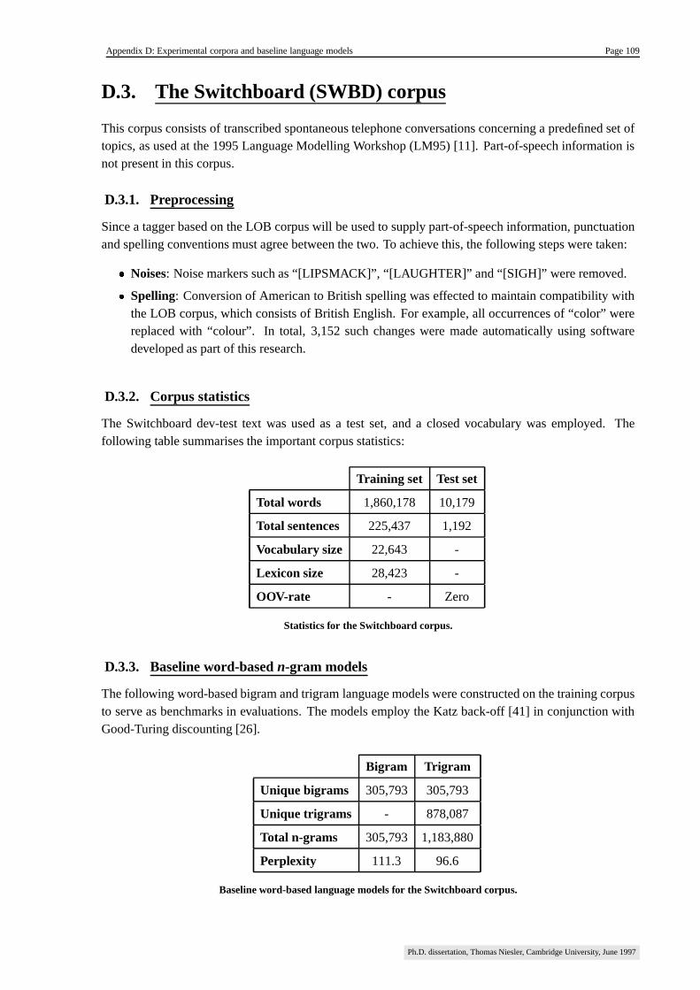
Appendix D: Experimental corpora and baseline language models Page 109
D.3. The Switchboard (SWBD) corpus
This corpus consists of transcribed spontaneous telephone conversations concerning a predefined set oftopics, as used at the 1995 Language Modelling Workshop (LM95) [11]. Part-of-speech information isnot present in this corpus.
D.3.1. Preprocessing
Since a tagger based on the LOB corpus will be used to supply part-of-speech information, punctuationand spelling conventions must agree between the two. To achieve this, the following steps were taken:
� Noises: Noise markers such as “[LIPSMACK]”, “[LAUGHTER]” and “[SIGH]” were removed.� Spelling: Conversion of American to British spelling was effected to maintain compatibility with
the LOB corpus, which consists of British English. For example, all occurrences of “color” werereplaced with “colour”. In total, 3,152 such changes were made automatically using softwaredeveloped as part of this research.
D.3.2. Corpus statistics
The Switchboard dev-test text was used as a test set, and a closed vocabulary was employed. Thefollowing table summarises the important corpus statistics:
Training set Test set
Total words 1,860,178 10,179
Total sentences 225,437 1,192
Vocabulary size 22,643 -
Lexicon size 28,423 -
OOV-rate - Zero
Statistics for the Switchboard corpus.
D.3.3. Baseline word-based n-gram models
The following word-based bigram and trigram language models were constructed on the training corpusto serve as benchmarks in evaluations. The models employ the Katz back-off [41] in conjunction withGood-Turing discounting [26].
Bigram Trigram
Unique bigrams 305,793 305,793
Unique trigrams - 878,087
Total n-grams 305,793 1,183,880
Perplexity 111.3 96.6
Baseline word-based language models for the Switchboard corpus.
Ph.D. dissertation, Thomas Niesler, Cambridge University, June 1997
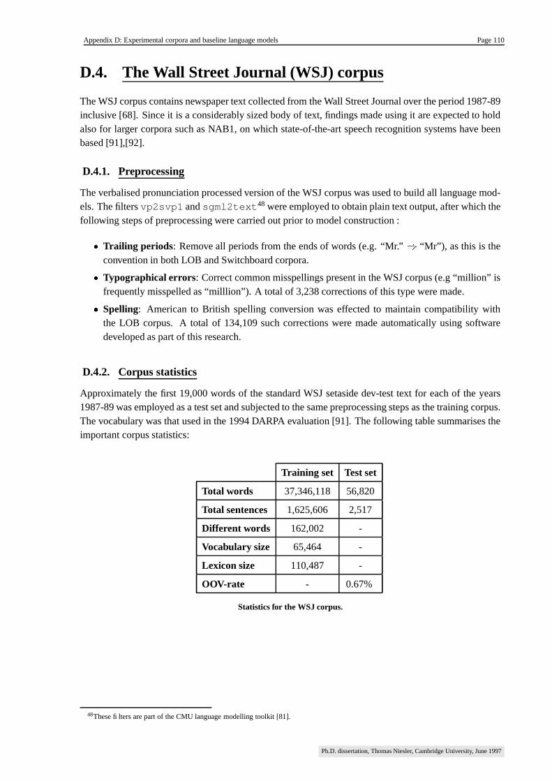
Appendix D: Experimental corpora and baseline language models Page 110
D.4. The Wall Street Journal (WSJ) corpus
The WSJ corpus contains newspaper text collected from the Wall Street Journal over the period 1987-89inclusive [68]. Since it is a considerably sized body of text, findings made using it are expected to holdalso for larger corpora such as NAB1, on which state-of-the-art speech recognition systems have beenbased [91],[92].
D.4.1. Preprocessing
The verbalised pronunciation processed version of the WSJ corpus was used to build all language mod-els. The filters vp2svp1 and sgml2text48 were employed to obtain plain text output, after which thefollowing steps of preprocessing were carried out prior to model construction :
� Trailing periods: Remove all periods from the ends of words (e.g. “Mr.” � “Mr”), as this is theconvention in both LOB and Switchboard corpora.
� Typographical errors: Correct common misspellings present in the WSJ corpus (e.g “million” isfrequently misspelled as “milllion”). A total of 3,238 corrections of this type were made.
� Spelling: American to British spelling conversion was effected to maintain compatibility withthe LOB corpus. A total of 134,109 such corrections were made automatically using softwaredeveloped as part of this research.
D.4.2. Corpus statistics
Approximately the first 19,000 words of the standard WSJ setaside dev-test text for each of the years1987-89 was employed as a test set and subjected to the same preprocessing steps as the training corpus.The vocabulary was that used in the 1994 DARPA evaluation [91]. The following table summarises theimportant corpus statistics:
Training set Test set
Total words 37,346,118 56,820
Total sentences 1,625,606 2,517
Different words 162,002 -
Vocabulary size 65,464 -
Lexicon size 110,487 -
OOV-rate - 0.67%
Statistics for the WSJ corpus.
48These filters are part of the CMU language modelling toolkit [81].
Ph.D. dissertation, Thomas Niesler, Cambridge University, June 1997

Appendix D: Experimental corpora and baseline language models Page 111
D.4.3. Baseline word-based n-gram models
The following word-based bigram and trigram language models were constructed on the training corpusto serve as benchmarks in evaluations. The models employ the Katz back-off [41] in conjunction withGood-Turing discounting [26].
Bigram Trigram
Unique bigrams 4,051,165 4,051,165
Unique trigrams - 9,548,230
Total n-grams 4,051,165 13,599,395
Perplexity 215.4 144.4
Baseline word-based language models for the WSJ corpus.
Ph.D. dissertation, Thomas Niesler, Cambridge University, June 1997

Appendix E: LOB corpus word-categories Page 112
Appendix E
LOB corpus word-categories
E.1. Part-of-speech tags found in the LOB corpus
The following table lists the grammatical word classifications found in the LOB corpus [40]. Punctuationsymbols have been omitted, and the tag “SE” referring to the end-of-sentence marker was added.
Category name Description&FW foreign wordABL pre-quantifier (quite, rather, such)ABN pre-quantifier (all, half)ABX pre-quantifier / double conjunction (both)AP post-determiner (few, fewer, former, last, latter, least, less, little, many,
more, most, much, next, only, other, own, same, several, very)AP$ other’sAPS othersAPS$ others’AT singular article (a, an, every)ATI singular or plural article (the, no)BE beBED wereBEDZ wasBEG beingBEM am, ’mBEN beenBER are, ’reBEZ is, ’sCC coordinating conjunction (and, and/or, but, nor, only, or, yet)CD cardinal (two, three, etc; hundred, thousand,etc; dozen, zero)CD$ cardinal + genitiveCD-CD hyphenated pair of cardinalsCD1 one, 1CD1$ one’sCD1S onesCDS cardinal + plural (tens, millions, dozens, etc)CS subordinating conjunction (after, although, etc)
Ph.D. dissertation, Thomas Niesler, Cambridge University, June 1997
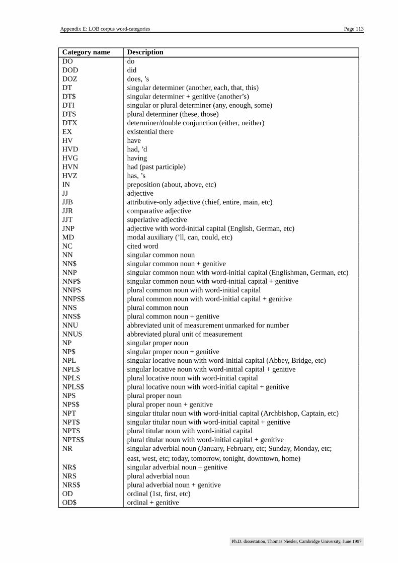
Appendix E: LOB corpus word-categories Page 113
Category name DescriptionDO doDOD didDOZ does, ’sDT singular determiner (another, each, that, this)DT$ singular determiner + genitive (another’s)DTI singular or plural determiner (any, enough, some)DTS plural determiner (these, those)DTX determiner/double conjunction (either, neither)EX existential thereHV haveHVD had, ’dHVG havingHVN had (past participle)HVZ has, ’sIN preposition (about, above, etc)JJ adjectiveJJB attributive-only adjective (chief, entire, main, etc)JJR comparative adjectiveJJT superlative adjectiveJNP adjective with word-initial capital (English, German, etc)MD modal auxiliary (’ll, can, could, etc)NC cited wordNN singular common nounNN$ singular common noun + genitiveNNP singular common noun with word-initial capital (Englishman, German, etc)NNP$ singular common noun with word-initial capital + genitiveNNPS plural common noun with word-initial capitalNNPS$ plural common noun with word-initial capital + genitiveNNS plural common nounNNS$ plural common noun + genitiveNNU abbreviated unit of measurement unmarked for numberNNUS abbreviated plural unit of measurementNP singular proper nounNP$ singular proper noun + genitiveNPL singular locative noun with word-initial capital (Abbey, Bridge, etc)NPL$ singular locative noun with word-initial capital + genitiveNPLS plural locative noun with word-initial capitalNPLS$ plural locative noun with word-initial capital + genitiveNPS plural proper nounNPS$ plural proper noun + genitiveNPT singular titular noun with word-initial capital (Archbishop, Captain, etc)NPT$ singular titular noun with word-initial capital + genitiveNPTS plural titular noun with word-initial capitalNPTS$ plural titular noun with word-initial capital + genitiveNR singular adverbial noun (January, February, etc; Sunday, Monday, etc;
east, west, etc; today, tomorrow, tonight, downtown, home)NR$ singular adverbial noun + genitiveNRS plural adverbial nounNRS$ plural adverbial noun + genitiveOD ordinal (1st, first, etc)OD$ ordinal + genitive
Ph.D. dissertation, Thomas Niesler, Cambridge University, June 1997

Appendix E: LOB corpus word-categories Page 114
Category name DescriptionPN nominal pronoun (anybody, anyone, anything; everybody, everyone,
everything; nobody, none, nothing; somebody, someone, something; so)PN$ nominal pronoun + genitivePP$ possessive determiner (my, your, etc)PP$$ possessive pronoun (mine, yours, etc)PP1A personal pronoun, 1st person singular nominative (I)PP1AS personal pronoun, 1st person plural nominative (we)PP1O personal pronoun, 1st person singular accusative (me)PP1OS personal pronoun, 1st person plural accusative (us, ’s)PP2 personal pronoun, 2nd person (you, thou, thee, ye)PP3 personal pronoun, 3rd person singular nominative + accusative (it)PP3A personal pronoun, 3rd person singular nominative (he,she)PP3AS personal pronoun, 3rd person plural nominative (they)PP3O personal pronoun, 3rd person singular accusative (him,her)PP3OS personal pronoun, 3rd person plural accusative (them, ’em)PPL singular reflexive pronounPPLS plural reflexive pronoun, reciprocal pronounQL qualifier (as, awfully, less, more, so, too, very, etc)QLP post-quantifier (enough, indeed)RB adverbRB$ adverb + genitive (else’s)RBR comparative adverbRBT superlative adverbRI adverb (homograph of preposition: below, near, etc)Rn nominal adverb (here, now, thee, then, etc)RP adverbial particle (back, down, off, etc)SE end-of-sencence markerTO infinitival toUH interjectionVB base form of verbVBD past tense of verbVBG present participle, gerundVBN past participleVBZ 3rd person singular of verbWDT WH-determiner (what, whatever, whatsoever, interrogative which,
whichever, whichsoever)WDTR WH-determiner relative (which)WP WH-pronoun, interrogative, nominative + accusative (who, whoever)WP$ WH-pronoun, interrogative, gen (whose)WP$R WH-pronoun, relative, gen (whose)WPA WH-pronoun, nominative (whosoever)WPO WH-pronoun, interrogative, accusative (whom, whomsoever)WPOR WH-pronoun, relative, accusative (whom)WPR WH-pronoun, relative, nominative + accusative (that, relative who)WRB WH-adverb (how, when, etc)XNOT not, n’tZZ letter of the alphabet (e, pi, x, etc)
Ph.D. dissertation, Thomas Niesler, Cambridge University, June 1997
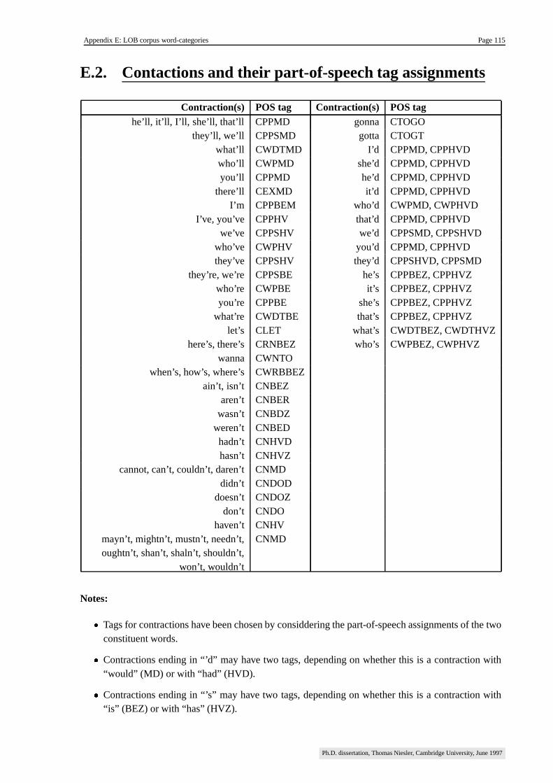
Appendix E: LOB corpus word-categories Page 115
E.2. Contactions and their part-of-speech tag assignments
Contraction(s) POS tag Contraction(s) POS taghe’ll, it’ll, I’ll, she’ll, that’ll CPPMD gonna CTOGO
they’ll, we’ll CPPSMD gotta CTOGTwhat’ll CWDTMD I’d CPPMD, CPPHVDwho’ll CWPMD she’d CPPMD, CPPHVDyou’ll CPPMD he’d CPPMD, CPPHVD
there’ll CEXMD it’d CPPMD, CPPHVDI’m CPPBEM who’d CWPMD, CWPHVD
I’ve, you’ve CPPHV that’d CPPMD, CPPHVDwe’ve CPPSHV we’d CPPSMD, CPPSHVD
who’ve CWPHV you’d CPPMD, CPPHVDthey’ve CPPSHV they’d CPPSHVD, CPPSMD
they’re, we’re CPPSBE he’s CPPBEZ, CPPHVZwho’re CWPBE it’s CPPBEZ, CPPHVZyou’re CPPBE she’s CPPBEZ, CPPHVZ
what’re CWDTBE that’s CPPBEZ, CPPHVZlet’s CLET what’s CWDTBEZ, CWDTHVZ
here’s, there’s CRNBEZ who’s CWPBEZ, CWPHVZwanna CWNTO
when’s, how’s, where’s CWRBBEZain’t, isn’t CNBEZ
aren’t CNBERwasn’t CNBDZ
weren’t CNBEDhadn’t CNHVDhasn’t CNHVZ
cannot, can’t, couldn’t, daren’t CNMDdidn’t CNDOD
doesn’t CNDOZdon’t CNDO
haven’t CNHVmayn’t, mightn’t, mustn’t, needn’t,oughtn’t, shan’t, shaln’t, shouldn’t,
won’t, wouldn’t
CNMD
Notes:
� Tags for contractions have been chosen by considdering the part-of-speech assignments of the twoconstituent words.
� Contractions ending in “’d” may have two tags, depending on whether this is a contraction with“would” (MD) or with “had” (HVD).
� Contractions ending in “’s” may have two tags, depending on whether this is a contraction with“is” (BEZ) or with “has” (HVZ).
Ph.D. dissertation, Thomas Niesler, Cambridge University, June 1997

Appendix F: OALD tag mappings Page 116
Appendix F
OALD tag mappings
An electronic version of the Oxford Advanced Learner’s Dictionary (OALD) containing sufficientlydetailed word tagging information was used to augment the lexicon extracted from the LOB corpus withthe purpose of reducing the OOV rate [50]. The following table lists the OALD tags used in this process,as well as the LOB tags to which they were mapped. In a few cases it was necessary to map an OALDtag to more than one LOB tag, this being indicated by separating the latter with colons.
OALD tag LOB tag OALD tag LOB tagGb VBG Ki NNGc VBD Kj NNSGd VBN K6 NNHa VBZ K7 NNHb VBG K8 NNHc VBD K9 NN : NNSHd VBN Lk NNH0 VB L@ NNH1 VB Mi NNH2 VB Mj NNSH3 VB M6 NNH4 VB M7 NNH5 VB M8 NNIa VBZ M9 NN : NNSIb VBG M@ NNIc VBD Nl NPId VBN Nm NPI0 VB Nn NPI1 VB No NPI2 VB OA JJI3 VB OB JJI4 VB OC JJI5 VB OD JJJa VBZ OE JJJb VBG Op JJJc VBD Oq JJBJd VBN Or JJRJ0 VB Os JJTJ1 VB Ot JJJ2 VB Pu RBJ3 VB P+ RPJ4 VB T- INJ5 VB W- UH
Ph.D. dissertation, Thomas Niesler, Cambridge University, June 1997

Appendix G: Trigger approximations Page 117
Appendix G
Trigger approximations
By virtue of the category-conditional probability function chosen to model occurrence correlations be-tween trigger and target words, the distribution function is :
� � � � � �� � � �"!#� $'& � � �� � � � � � � � 1 � � � � � � ��� � � � 1 � � (132)
where
� � is the distance separating trigger and target.
� � � is the probability of occurrence of the trigger.
� � � , � and � are the parameters describing the transient occurrence probability of the targetwith respect to a trigger sighting.
� � is a normalising constant.
This appendix describes the two-stage algebraic approximation of (132) by a distribution of the form
�� � � � � � ���� ! ��� � ! �� � ! ��� & ��� � & � � � & �
G.1. First approximation
The objective here is to eliminate the product operator from equation (132), since its presence makesalgebraic manipulation difficult. Consider the first term on the right-hand side of (132) :
� �"!#� $'& � � � � � � � � � � 1 � ��� ��� � � � � � � � � �"!#� $'& � � �� � � � 1 � � �where
� � �� � � � � (133)
Ph.D. dissertation, Thomas Niesler, Cambridge University, June 1997

Appendix G: Trigger approximations Page 118
Take the logarithm and apply the first-order Taylor approximation �� ��� � � � � � to find:
�� � � �"!#� $'& � � � � � � � � � � 1 � � � � � �� ��� � � � � � � �"!� � $'& � � � � 1 �� � �� ��� � � � � � � � � � � � 1 � �� � � �
Now, take the inverse logarithm and resubstitute (133) into the above we obtain:
��"!#� $'& � � � � � � � � � � 1 � � � ��� � � � � � � � � � � � � = ;� ;���� � �6 = ;�� � ;��� > � 6 = ;� ;�� > � (134)
For clarity now define:
� � � ��6 = ;�� � ;�� >�� 6 = ;� ;�� >
(135)
and it follows from (132), (134) and (135) that:
� � � � � �� � � � � �� � � � ��� � � � 1 � � ��� � � � � � � � !�� �;���� �
(136)
This approximation is good when�
!��@� �
@ �� �, which is true when
� � � �,� �
��
and � ��, as
may be expected for content words.
G.2. Second approximation
Since we would ultimately like to find closed-form expressions for the approximate mean and mean-square of the probability distribution (132), and this is not yet possible using (136), we will furtherapproximate the latter by:
�� � � � � � ��� ! ��� �
! �� � ! ��� & ��� � & � � � & � (137)
where
� � � ! ��� & � � � (138)
The functional form of (137) has the following motivations:
� As the superposition of two geometric terms, it retains the overall geometric character exhibitedempirically by the distribution � � � � .� The faster geometric component should model the initially more rapid decay of theobserved distribution (which is in turn due to the higher conditional probability at small � ).� The slower geometric component should model the tail of the observed distribution.� Closed form expressions for the mean and mean-square exist.
Ph.D. dissertation, Thomas Niesler, Cambridge University, June 1997

Appendix G: Trigger approximations Page 119
Note firstly that��� $'& �� � � � � �and that for
� � � & � � and� � � ! � � :
� � �� � � � � � � � � ��� � � ������ �� �so that equation (137) represents a valid probability mass function. In order to solve for the parametersof (137) in terms of the parameters of (136), we impose the following three constraints :
1. Equality in the limit as � � �: From (136) we find that:
����� � � �� � � � ���� � � ��� � � � � � � �
and from (137), assuming� & � � ! :
����� � � �� � � � � � �� & ��� � & � � � &and so by requiring
����� � � �� � � � � ����� ��� �� � � �we may choose
� & � � � � � � (139)
and
� & � � � �� � � � � (140)
2. Equality at � � � : From (136) we find that:
�� ��� � ��� ��� � ��� �and from (137) :
�� ��� � ��� ��� ! �! ��� & � & �
so that, for�� ��� � � �� ��� � we find
�! �
� � � � � & � &� !
(141)
Ph.D. dissertation, Thomas Niesler, Cambridge University, June 1997

Appendix G: Trigger approximations Page 120
3. Equality of the first derivative at � � � : From (136) we find that:
�
� ��� � � � ���
� � � � � � � � �� ��� � � � � � � � � � � � � � � �� �� � � � � � � � � � � � � � � � � � � � ��� � � �� � � � � !��
� ;�� �
from which, taking � � � , we obtain:
�
� � �� � � � ���� � $'& ��� � � � � ��� � ����� � �� ��� � � � � � � � ��� � ��� �� � �� � � � � (142)
Similarly, from (137):
�
� ��� � � � ��� � � ! � �� ��� �� ! � ��� �� ! �
� � ! � � & � �� ��� � & �� ��� � & � � � & �from which, taking � � � , we obtain:
�
� � �� � � � ���� � $'& ��� � � ! � �� ��� �� ! � � ! ��� & � �� ��� � & � � & � (143)
Using (139) and (140) we may write:
� & �� ��� � & �� � & � � � �� � � � � � �� ��� � & � ��� � � � � �� � � � � �� ��� � & � (144)
Now, by requiring:
�
� � �� � � � ���� � $'& �
�
� ��� � � � �
��� � $'&
we find from (139), (141), (142), (143) and (144) that:
� ! � �� ��� � ! � � ! � �� ��� � & � �� � � ��� � � � � � � �� ��� � ����� � �� � � � � �� ��� � ��� � � � � � �� ��� � ! � � �� ��� �� & � �� � � � � � � � ��� � �� ��� � ������ � �� � � � � �� �� ��� � ! � �
�� ��� � & �� � � � ��� � � � � � � � � � � � � �� � �� � � � � �� � ��� � � �� �� ��� � & � � � � � � � ��� � � �� � � � �� � ��� � � �
so that, finally, we obtain:
�! �
� ��� �� & �� � � ����� � � � � � � � � 6 � > ;����� � ��;���� � �(145)
Ph.D. dissertation, Thomas Niesler, Cambridge University, June 1997

Appendix H: The truncated geometric distribution Page 121
Appendix H
The truncated geometricdistribution
Consider an experiment consisting of Bernoulli trials with probability of success�� . The number of
repetitions before witnessing the first positive result is described by the geometric distribution:
� � � � � � � � ��� �� � � � � (146)
Now select the subset of trials for which � � � , where � is an integer greater than zero. The probabilitydistribution over this interval
��� � � may be determined by applying the normalisation requirement
��"!�� $'& ��� � � � �
to equation (146) and obtaining:
��� � � � � � � � � � ���"!3� $'& � � � � � � �
� ��� �� � � � �� ���� �
� � � with � � � � � ������ � �� � (147)
In this appendix we find expressions for the mean and mean-square of this truncated geometric distri-bution, and begin by calculating the moment generating function:
� ��� � � ��"!�� $'& � � 1 � ��� � �
� ��� ���� ��
� � � ��"!�� $'& ��� � � � � � � 1 �
� �� � � � � � ��� � � � � � �� � ���� ��
� � � � � � � � ��� �� � � ���� �
� � � ��� � � � � �� � � ��� �� � � (148)
Ph.D. dissertation, Thomas Niesler, Cambridge University, June 1997

Appendix H: The truncated geometric distribution Page 122
where:
� � ��� � ���� �
� � � �Taking the derivative of (148) with respect to
�we find:
�
� � � ��� � � � � � ��� � � � � � � � 1 � ��� � � � � � � � � � ��� � � � � � � � � ��� � � � �� � � � ��� � � � � �
� � �� ��� � � � � � � 1 � ��� � � � � � � � � � � � � �
!�� � ��� � � � � �
!� � � � ��� � � � � �and to obtain the mean � ��� � � � we set
� � � :
� ��� � � � � �
� � � ��� � ���� � $'&
� � ��� ��
� � � � � ��� ��� � � � ! � � � �� �� ��� � � � � � �� �
�
(149)
Taking the second derivative of (148) with respect to�
we find:
������ ����� � � ���� ������� " � ��� � � � � � �� � " � ��� � � � � � � � " � ��� � � � ��
� � ��� � � � � � � ��� �� . � " � ��� � � � �� ."!� ����� " � ��� � � � �$#��% &�' �(� " � ��� � � � � � � " � ��� � � � �
� � �)� �* � � �� . � " � ��� � � � �� .+! � ����� " � ��� �-, � � � " � ��� � � �� ����� " � ��� � � � �-#
and obtain the mean-square ! ��� � � � of the distribution by again setting� � � :
! ��� � � � � � �� � � � ��� � �
���� � $'&
� � � �� � ��� � � � � � � � ��� � � � � �"! � � � � �� � � � � � ��� � � � � ���� �
�
� � � � ��� �
� � � � � ��� �� � � � � ! � � � �� �� ��� �� � � � � � � � ��� � � �� �
�
(150)
Ph.D. dissertation, Thomas Niesler, Cambridge University, June 1997