machine learning - a. supervised learning a.3. regularization · xn i=1 log p(y i jx i; )! + xp j=1...
TRANSCRIPT

Machine Learning
Machine LearningA. Supervised Learning
A.3. Regularization
Lars Schmidt-Thieme
Information Systems and Machine Learning Lab (ISMLL)Institute for Computer Science
University of Hildesheim, Germany
Lars Schmidt-Thieme, Information Systems and Machine Learning Lab (ISMLL), University of Hildesheim, Germany
1 / 23

Machine Learning
SyllabusFri. 21.10. (1) 0. Introduction
A. Supervised LearningFri. 28.10. (2) A.1 Linear Regression
Fri. 4.11. (3) A.2 Linear ClassificationFri. 11.11. (4) A.3 RegularizationFri. 18.11. (5) A.4 High-dimensional DataFri. 25.11. (6) A.5 Nearest-Neighbor Models
Fri. 2.12. (7) A.6 Support Vector MachinesFri. 9.12. (8) A.7 Decision Trees
Fri. 16.12. (9) A.8 A First Look at Bayesian and Markov Networks
B. Unsupervised LearningFri. 13.1. (10) B.1 ClusteringFri. 20.1. (11) B.2 Dimensionality ReductionFri. 27.1. (12) B.3 Frequent Pattern Mining
C. Reinforcement LearningFri. 3.2. (13) C.1 State Space Models
(14) C.2 Markov Decision Processes
Lars Schmidt-Thieme, Information Systems and Machine Learning Lab (ISMLL), University of Hildesheim, Germany
1 / 23

Machine Learning
Outline
1. The Problem of Overfitting
2. Model Selection
3. Regularization
4. Hyperparameter Optimization
Lars Schmidt-Thieme, Information Systems and Machine Learning Lab (ISMLL), University of Hildesheim, Germany
1 / 23

Machine Learning 1. The Problem of Overfitting
Outline
1. The Problem of Overfitting
2. Model Selection
3. Regularization
4. Hyperparameter Optimization
Lars Schmidt-Thieme, Information Systems and Machine Learning Lab (ISMLL), University of Hildesheim, Germany
1 / 23

Machine Learning 1. The Problem of Overfitting
Fitting of models
●
●
●
●
●
●
●
●
●
●
●
●
●
●
●●
●●
●
●
●
●
●
●
●
●
●
●
●
●
●
●
●
●
●
●
●
●
●
●
●
●
●●
●
●
●●
●
●
5 10 15 20 25
020
4060
8010
012
0
Linear model (RSS= 11353.52 )
Speed
Bre
akin
g di
stan
ce
●
●
●
●
●
●
●
●
●
●
●
●
●
●
●●
●●
●
●
●
●
●
●
●
●
●
●
●
●
●
●
●
●
●
●
●
●
●
●
●
●
●●
●
●
●●
●
●
5 10 15 20 25
020
4060
8010
012
0
Quadratic model (RSS= 10824.72 )
Speed
Bre
akin
g di
stan
ce
●
●
●
●
●
●
●
●
●
●
●
●
●
●
●●
●●
●
●
●
●
●
●
●
●
●
●
●
●
●
●
●
●
●
●
●
●
●
●
●
●
●●
●
●
●●
●
●
5 10 15 20 25
020
4060
8010
012
0
Polynomial model (RSS= 7029.37 )
Speed
Bre
akin
g di
stan
ce
Lars Schmidt-Thieme, Information Systems and Machine Learning Lab (ISMLL), University of Hildesheim, Germany
1 / 23

Machine Learning 1. The Problem of Overfitting
Underfitting/OverfittingUnderfitting:
I the model is not complex enough to explain the data well.
I results in poor predictive performance.
Overfitting:I the model is too complex, it describes the
I noise instead of theI underlying relationship between target and predictors.
I results in poor predictive performance as well.
Remark: Given N points (xn, yn) without repeated measurements (i.e.xn 6= xm, n 6= m), there exists a polynomial of degree N − 1 with RSSequal to 0.
Lars Schmidt-Thieme, Information Systems and Machine Learning Lab (ISMLL), University of Hildesheim, Germany
2 / 23

Machine Learning 2. Model Selection
Outline
1. The Problem of Overfitting
2. Model Selection
3. Regularization
4. Hyperparameter Optimization
Lars Schmidt-Thieme, Information Systems and Machine Learning Lab (ISMLL), University of Hildesheim, Germany
3 / 23

Machine Learning 2. Model Selection
Model Selection MeasuresModel selection means: we have a set of models, e.g.,
Y =
p−1∑i=0
βiXi
indexed by p (i.e., one model for each value of p), make a choice whichmodel describes the data best.If we just look at losses / fit measures such as RSS, then
the larger p, the better the fit
or equivalently
the larger p, the lower the loss
as the model with p parameters can be reparametrized in a model withp′ > p parameters by setting
β′i =
{βi , for i ≤ p0, for i > p
Lars Schmidt-Thieme, Information Systems and Machine Learning Lab (ISMLL), University of Hildesheim, Germany
3 / 23

Machine Learning 2. Model Selection
Model Selection MeasuresOne uses model selection measures of type
model selection measure = fit− complexity
or equivalently
model selection measure = loss + complexity
The smaller the loss (= lack of fit), the better the model.
The smaller the complexity, the simpler and thus better the model.
The model selection measure tries to find a trade-off between fit/loss andcomplexity.
Lars Schmidt-Thieme, Information Systems and Machine Learning Lab (ISMLL), University of Hildesheim, Germany
4 / 23
Machine Learning 2. Model Selection
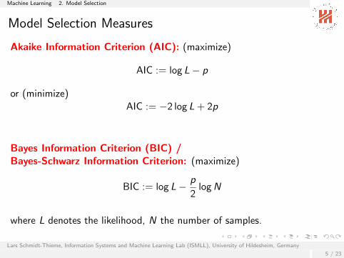
Model Selection Measures
Akaike Information Criterion (AIC): (maximize)
AIC := log L− p
or (minimize)AIC := −2 log L + 2p
Bayes Information Criterion (BIC) /Bayes-Schwarz Information Criterion: (maximize)
BIC := log L− p
2logN
where L denotes the likelihood, N the number of samples.
Lars Schmidt-Thieme, Information Systems and Machine Learning Lab (ISMLL), University of Hildesheim, Germany
5 / 23

Machine Learning 2. Model Selection
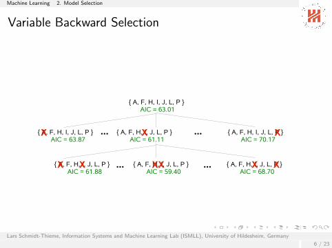
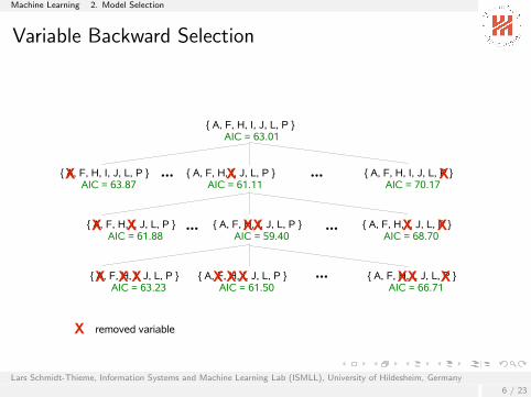
Variable Backward Selection
{ A, F, H, I, J, L, P } AIC = 63.01
{ A, F, H, I, J, L, P }AIC = 63.87
{ A, F, H, I, J, L, P }AIC = 61.11
{ A, F, H, I, J, L, P }AIC = 70.17
X
X X X... ...
{ A, F, H, I, J, L, P }AIC = 61.88
{ A, F, H, I, J, L, P }AIC = 59.40
{ A, F, H, I, J, L, P }AIC = 68.70
... ...X X X XX X
{ A, F, H, I, J, L, P }AIC = 63.23
{ A, F, H, I, J, L, P }AIC = 61.50
{ A, F, H, I, J, L, P }AIC = 66.71
...XXX X XX XX X
removed variable
Lars Schmidt-Thieme, Information Systems and Machine Learning Lab (ISMLL), University of Hildesheim, Germany
6 / 23

Machine Learning 2. Model Selection
Variable Backward Selection
{ A, F, H, I, J, L, P } AIC = 63.01
{ A, F, H, I, J, L, P }AIC = 63.87
{ A, F, H, I, J, L, P }AIC = 61.11
{ A, F, H, I, J, L, P }AIC = 70.17
X
X X X... ...
{ A, F, H, I, J, L, P }AIC = 61.88
{ A, F, H, I, J, L, P }AIC = 59.40
{ A, F, H, I, J, L, P }AIC = 68.70
... ...X X X XX X
{ A, F, H, I, J, L, P }AIC = 63.23
{ A, F, H, I, J, L, P }AIC = 61.50
{ A, F, H, I, J, L, P }AIC = 66.71
...XXX X XX XX X
removed variableLars Schmidt-Thieme, Information Systems and Machine Learning Lab (ISMLL), University of Hildesheim, Germany
6 / 23
Machine Learning 2. Model Selection
Variable Backward Selection
{ A, F, H, I, J, L, P } AIC = 63.01
{ A, F, H, I, J, L, P }AIC = 63.87
{ A, F, H, I, J, L, P }AIC = 61.11
{ A, F, H, I, J, L, P }AIC = 70.17
X
X X X... ...
{ A, F, H, I, J, L, P }AIC = 61.88
{ A, F, H, I, J, L, P }AIC = 59.40
{ A, F, H, I, J, L, P }AIC = 68.70
... ...X X X XX X
{ A, F, H, I, J, L, P }AIC = 63.23
{ A, F, H, I, J, L, P }AIC = 61.50
{ A, F, H, I, J, L, P }AIC = 66.71
...XXX X XX XX X
removed variable
Lars Schmidt-Thieme, Information Systems and Machine Learning Lab (ISMLL), University of Hildesheim, Germany
6 / 23

Machine Learning 3. Regularization
Outline
1. The Problem of Overfitting
2. Model Selection
3. Regularization
4. Hyperparameter Optimization
Lars Schmidt-Thieme, Information Systems and Machine Learning Lab (ISMLL), University of Hildesheim, Germany
7 / 23

Machine Learning 3. Regularization
Shrinkage
Model selection operates by
I fitting models for a set of models with varying complexity and thenpicking the ”best one” ex post,
I omitting some parameters completely (i.e. forcing them to be 0).
Shrinkage follows a similar idea:
I smaller parameters mean a simpler hypothesis/less complex model.Hence, small parameters should be prefered in general.
I a term is added to the model equation to penalize high parametersinstead of forcing them to be 0.
Lars Schmidt-Thieme, Information Systems and Machine Learning Lab (ISMLL), University of Hildesheim, Germany
7 / 23

Machine Learning 3. Regularization
Shrinkage
There are various types of shrinkage techniques for different applicationdomains.
L1/Lasso Regularization: λ∑p
j=1
∣∣∣βj ∣∣∣ = λ∥∥∥β∥∥∥
1
L2/Tikhonov Regularization: λ∑p
j=1 β2j = λ
∥∥∥β∥∥∥2
2
Elastic Net: λ1
∥∥∥β∥∥∥1
+ λ2
∥∥∥β∥∥∥2
2
Lars Schmidt-Thieme, Information Systems and Machine Learning Lab (ISMLL), University of Hildesheim, Germany
8 / 23

Machine Learning 3. Regularization
Ridge Regression
Ridge regression is a combination of
n∑i=1
(yi − yi )2
︸ ︷︷ ︸+λ
p∑j=1
β2j︸ ︷︷ ︸
= L2 loss +λ L2 regularization
Lars Schmidt-Thieme, Information Systems and Machine Learning Lab (ISMLL), University of Hildesheim, Germany
9 / 23

Machine Learning 3. Regularization
Ridge Regression (Closed Form)Ridge regression: minimize
RSSλ(β) =RSS(β) + λ
p∑j=1
β2j = 〈y − Xβ, y − Xβ〉+ λ
p∑j=1
β2j
⇒ β =(
XTX + 2λI)−1
XTy, I :=
1 0 · · · 0
0 1. . .
......
. . .. . . 0
0 · · · 0 1
with λ ≥ 0 a complexity parameter / regularization parameter.
As solutions of ridge regression are not equivariant under scaling of thepredictors, data is normalized before ridge regression:
x ′i ,j :=xi ,j − x.,jσ(x.,j)
Lars Schmidt-Thieme, Information Systems and Machine Learning Lab (ISMLL), University of Hildesheim, Germany
10 / 23

Machine Learning 3. Regularization
Ridge Regression (Gradient Descent)1: procedure Ridge-Regr-
GD(y : RP → R, β(0) ∈ RP+1, α, tmax ∈ N,X ∈ RN×P , y ∈ RN)2: for t = 1, . . . , tmax do
3: β(t)0 := β
(t−1)0 − α
(2∑N
n=1− (yn − y (Xn)))
4: for j = 1, . . . ,P do5:
β(t)j := β
(t−1)j − α
(2∑N
n=1−Xn,j (yn − y (Xn)) + 2λβ(t−1)j
)6: if converged then7: return β(t)
L2-Regularized Update Rule
β(t)j := (1− 2αλ)︸ ︷︷ ︸
shrinkage
β(t−1)j − α
(2
N∑n=1
−Xn,j (yn − y (Xn))
)
Lars Schmidt-Thieme, Information Systems and Machine Learning Lab (ISMLL), University of Hildesheim, Germany
11 / 23

Machine Learning 3. Regularization
Tikhonov Regularization Derivation (1/2)Treat the true parameters θj as random variables Θj with the followingdistribution (prior):
Θj ∼ N (0, σΘ), j = 1, . . . , p
Then the joint likelihood of the data and the parameters is
LD,Θ(θ) :=
(n∏
i=1
p(xi , yi | θ)
)p∏
j=1
p(Θj = θj)
and the conditional joint log likelihood of the data and the parameters
log LcondD,Θ (θ) :=
(n∑
i=1
log p(yi | xi , θ)
)+
p∑j=1
log p(Θj = θj)
and
log p(Θj = θj) = log1√
2πσΘ
e−
θ2j
2σ2Θ = − log(
√2πσΘ)−
θ2j
2σ2Θ
Lars Schmidt-Thieme, Information Systems and Machine Learning Lab (ISMLL), University of Hildesheim, Germany
12 / 23
Machine Learning 3. Regularization
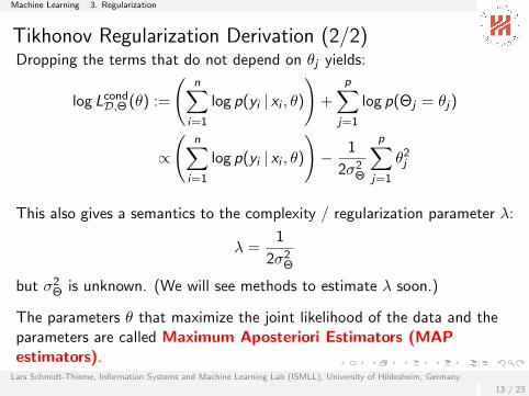
Tikhonov Regularization Derivation (2/2)Dropping the terms that do not depend on θj yields:
log LcondD,Θ (θ) :=
(n∑
i=1
log p(yi | xi , θ)
)+
p∑j=1
log p(Θj = θj)
∝
(n∑
i=1
log p(yi | xi , θ)
)− 1
2σ2Θ
p∑j=1
θ2j
This also gives a semantics to the complexity / regularization parameter λ:
λ =1
2σ2Θ
but σ2Θ is unknown. (We will see methods to estimate λ soon.)
The parameters θ that maximize the joint likelihood of the data and theparameters are called Maximum Aposteriori Estimators (MAPestimators).
Lars Schmidt-Thieme, Information Systems and Machine Learning Lab (ISMLL), University of Hildesheim, Germany
13 / 23

Machine Learning 3. Regularization
L2-Regularized Logistic Regression (Gradient Descent)
log LcondD (β) =
n∑i=1
yi 〈xi , β〉 − log(1 + e〈xi ,β〉)−2λP∑j=1
β2j
1: procedure Log-Regr-GA(Lcond
D : RP+1 → R, β(0) ∈ RP+1, α, tmax ∈ N, ε ∈ R+)2: for t = 1, . . . , tmax do
3: β(t)0 := β
(t−1)0 + α
∑ni=1
(yi − p
(Y = 1|X = xi ; β
(t−1)))
4: for j = 1, . . . ,P do
5: β(t)j :=
β(t−1)j + α(
∑ni=1 xi ,j
(yi − p
(Y = 1|X = xi ; β
(t−1)))−2λβ
(t−1)j )
6: if LcondD (β(t−1))− Lcond
D (β(t))) < ε then7: return β(t)
8: error ”not converged in tmax iterations”
Lars Schmidt-Thieme, Information Systems and Machine Learning Lab (ISMLL), University of Hildesheim, Germany
14 / 23

Machine Learning 3. Regularization
L2-Regularized Logistic Regression (Newton)
Newton update rule:
β(t) := β(t−1) + αH−1∇βp(Y = 1|X = xi ; β
(t−1))
pi = p(Y = 1|X = xi ; β
(t−1))
∇βLcondD =
∑n
i=1− (yi − pi )∑ni=1−xi ,1 (yi − pi )−2λβ1
...∑ni=1−xi ,P (yi − pi )−2λβP
H =
n∑i=1
−pi (1− pi ) xixTi −2λI
Lars Schmidt-Thieme, Information Systems and Machine Learning Lab (ISMLL), University of Hildesheim, Germany
15 / 23
Machine Learning 4. Hyperparameter Optimization
Outline
1. The Problem of Overfitting
2. Model Selection
3. Regularization
4. Hyperparameter Optimization
Lars Schmidt-Thieme, Information Systems and Machine Learning Lab (ISMLL), University of Hildesheim, Germany
16 / 23

Machine Learning 4. Hyperparameter Optimization
What is Hyperparameter Optimization?
Many learning algorithms Aλ have hyperparameters λ (learning rate,regularization). After choosing them, Aλ can be used to map the trainingdata Dtrain to a function y by minimizing some loss L(x ; y).
Identifying good values for the hyperparameters λ is calledhyperparameter optimization.
Hence, hyperparameter optimization is a second level optimization
argminλ∈Λ1
|Dcalib|∑
x∈Dcalib
L (x ;Aλ (Dtrain)) = argminλ∈ΛΨ(λ)
where Ψ is the hyperparameter response function and Dcalib acalibration set.
Lars Schmidt-Thieme, Information Systems and Machine Learning Lab (ISMLL), University of Hildesheim, Germany
16 / 23

Machine Learning 4. Hyperparameter Optimization
Why Hyperparameter Optimization
I So far only model parameters were optimized.
I Hyperparameters (such as regularization λ and learning rate α) came“out of the blue”.
I Hyperparameters can have a big impact on the prediction quality.
Lars Schmidt-Thieme, Information Systems and Machine Learning Lab (ISMLL), University of Hildesheim, Germany
17 / 23

Machine Learning 4. Hyperparameter Optimization
Grid SearchI Choose for each hyperparameter a set of values Λ1, . . . ,Λq.I Λ =
∏qi=1 Λi is then the combination of all hyperparameters in all Λi s.
I Then choose the hyperparameter λ ∈ Λ with best performance onDcalib.
●● ● ●●● ● ●
●● ● ●
●● ● ●
0.00 0.02 0.04 0.06 0.08 0.10
0.00
0.02
0.04
0.06
0.08
0.10
learning rate
regu
lariz
atio
n
Lars Schmidt-Thieme, Information Systems and Machine Learning Lab (ISMLL), University of Hildesheim, Germany
18 / 23

Machine Learning 4. Hyperparameter Optimization
Random SearchI Instead of choosing hyperparameters on a grid, choose random
hyperparameters λ for Λ (within a reasonable space).I Provides better results than grid search in cases of insensitive
hyperparameters.
●
●
●
●
●
●
●
●
●
●
●
●
●
●
●
●
●
●
●
●
●
●
●
●
●
0.2 0.4 0.6 0.8 1.0
0.0
0.2
0.4
0.6
0.8
learning rate
regu
lariz
atio
n
Lars Schmidt-Thieme, Information Systems and Machine Learning Lab (ISMLL), University of Hildesheim, Germany
19 / 23
Machine Learning 4. Hyperparameter Optimization
What is the Calibration Data?
Whenever a learning process depends on a hyperparameter, thehyperparameter can be estimated by picking the value with the lowesterror.
If this is done on test data, one actually uses test data in the trainingprocess (“train on test”), thereby lessen its usefullness for estimating thetest error.
Therefore, one splits the training data again in
I (proper) training data and
I calibration data.
The calibration data figures as test data during the training process.
Lars Schmidt-Thieme, Information Systems and Machine Learning Lab (ISMLL), University of Hildesheim, Germany
20 / 23

Machine Learning 4. Hyperparameter Optimization
Cross Validation
Instead of a single split into
training data, (validation data,) and test data
cross validation splits the data in k parts (of roughly equal size)
D = D1 ∪ D2 ∪ · · · ∪ Dk , Di pairwise disjunct
and averages performance over k learning problems
D(i)train = D \ Di , D
(i)test = Di i = 1, . . . , k
Common is 5- and 10-fold cross validation.
n-fold cross validation is also known as leave one out.
Lars Schmidt-Thieme, Information Systems and Machine Learning Lab (ISMLL), University of Hildesheim, Germany
21 / 23

Machine Learning 4. Hyperparameter Optimization
Cross Validation
How many folds to use in k-fold cross validation?
k = n / leave one out:
I approximately unbiased for the true prediction error.
I high variance as the n training sets are very similar.
I in general computationally costly as n different modelshave to be learnt.
k = 5:
I lower variance.
I bias could be a problem,due to smaller training set size the prediction error couldbe overestimated.
Lars Schmidt-Thieme, Information Systems and Machine Learning Lab (ISMLL), University of Hildesheim, Germany
22 / 23

Machine Learning 4. Hyperparameter Optimization
SummaryI The problem of underfitting can be overcome by using
more complex models, e.g., havingI variable interactions as in polynomial models.
I The problem of overfitting can be overcome byI model / variable selection as well as byI (parameter) shrinkage.
I Applying L2-regularization to Linear and Logistic Regression requiresonly few changes in the learning algorithm
I Shrinkage introduces a hyperparameter λ that cannot be learned bydirect loss minimization.
I Estimating the best hyperparameters can be considered as ameta-learning problem. They can be estimated e.g. by
I Grid Search orI Random Search.
using validation data.Lars Schmidt-Thieme, Information Systems and Machine Learning Lab (ISMLL), University of Hildesheim, Germany
23 / 23

Machine Learning
Further Readings
I [JWHT13, chapter 3], [Mur12, chapter 7], [HTFF05, chapter 3].
Lars Schmidt-Thieme, Information Systems and Machine Learning Lab (ISMLL), University of Hildesheim, Germany
24 / 23

Machine Learning
References
Trevor Hastie, Robert Tibshirani, Jerome Friedman, and James Franklin.
The elements of statistical learning: data mining, inference and prediction, volume 27.2005.
Gareth James, Daniela Witten, Trevor Hastie, and Robert Tibshirani.
An introduction to statistical learning.Springer, 2013.
Kevin P. Murphy.
Machine learning: a probabilistic perspective.The MIT Press, 2012.
Lars Schmidt-Thieme, Information Systems and Machine Learning Lab (ISMLL), University of Hildesheim, Germany
25 / 23