machine learning algorithms for image classification of ... · machine learning algorithms for...

International Research Journal of Engineering and Technology (IRJET) e-ISSN: 2395-0056

Volume: 04 Issue: 12 | Dec-2017 www.irjet.net p-ISSN: 2395-0072

© 2017, IRJET | Impact Factor value: 6.171 | ISO 9001:2008 Certified Journal | Page 640

Machine Learning algorithms for Image Classification of hand digits and face recognition dataset

Tanmoy Das1

1Masters in Industrial Engineering, Florida State University, Florida, United States of America ---------------------------------------------------------------------***--------------------------------------------------------------------

Abstract - In this research endeavor, the basis of several machine learning algorithms for image classification has been documented. The implementation of five classification schemes, e.g. Nearest Class Centroid classifier, Nearest Sub-class Centroid classifier using the number of classes in the subclasses in the set, Nearest Neighbor classifier, Perceptron trained using Backpropagation, Perceptron trained using MSE, has been reported. The performance of the schemes is also compared. The implementation has been performed in Python or Matlab. Key Words: Machine Learning; Image Classification; nearest neighbor classifier, nearest centroid classifier, Perceptron

1. INTRODUCTION Classification is a machine learning problem about how to assign labels to new data based on a given set of labeled data. The classification methods involves predicting a certain outcome based on a given input. In order to predict the outcome, the algorithm processes a training set containing a set of attributes and the respective outcome, usually called goal or prediction attribute. The classification algorithm assigns pixels in the image to categories or classes of interest. There are two types of classification algorithms e.g supervised, and unsupervised. Supervised classification uses the spectral signatures obtained from training samples otherwise data to classify an image or dataset. Unsupervised classification discovers spectral classes in a multiband image without the analyst’s intervention. The Image Classification algorithms aid in unsupervised classification by providing technology to create the clusters, competence to inspect the quality of the clusters, and access to classification algorithms. There are several algorithms developed by researchers over the years. In order to classify a set of data into different classes or categories, the relationship between the data and the classes into which they are classified must be well understood. In this paper, five algorithms will be discussed. In Section II, the explanation of different classification scheme will be provided, in Section III and IV database, & experimental methods are explained. Result, discussion and conclusion regarding the machine learning algorithms on different dataset are provided in the later sections.

2. DESCRIPTION OF THE CLASSIFICATION SCHEMES USED IN THIS EXPERIMENT There are five machine learning algorithm which are explored in this research work. The mathematical model behind these algorithms is illustrated in this section.

A. Nearest Class Centroid (NCC) classifier A firm algorithm for image classification is nearest class centroid classifier. In machine learning, a NCC is a classification model that allocates to observations the label of the class of training samples whose mean (centroid) is closest to the observation. In this classifier, each class is characterized by its centroid, with test samples classified to the class with the nearest centroid. When applied to text classification using vectors to represent documents, the NCC classifier is known as the Rocchio classifier because of its similarity to the Rocchio [1] algorithm. Given a set of data and their relationship, more details about the NCC centroid classifier can be found in [2, 3, 4, 5]. For each set of data point belonging to the same class, we compute their centroid vectors. If there are k classes in the training set, this leads to k centroid vectors }, where each is the centroid for the ith class [6]. Based on these similarities, we assign x to the class consistent to the most similar centroid. That is, the class of x is given by

The resemblance between two centroid vectors and between a document and a centroid vector are calculated using the cosine measure. In the first case,

( )

|| || || ||

whereas in the second case,

|| || || ||

|| ||




B. Nearest Sub Class (NSC) Centroid classifier using the number of classes in the subclasses in the set

Nearest Sub Class Classifier is a classification algorithm that unifies the flexibility of the nearest neighbor classifier with the robustness of the nearest mean classifier. The algorithm is based on the Maximum Variance Cluster algorithm and, as such, it belongs to the class of prototype-based classifiers. The variance constraint parameter of the cluster algorithm serves to regularize the classifier, that is, to prevent over-fitting. The MVC is a partitional cluster algorithm [7, 8] that aims at minimizing the squared error for all objects with respect to their cluster mean. Besides minimizing the squared error, it imposes a joint variance constraint on any two clusters. The joint variance constraint parameter prevents the trivial solution where every cluster contains exactly one object. Moreover, the joint variance constraint generally leads to clustering where the variance of every cluster is lower than the variance constraint value. According to the MVC model [9], a valid clustering of X into a set of clusters where Ci ⊆ X and M is the number of clusters, is the result of minimizing the squared error criterion, which is defined as

∑

Subject to the joint variance constraint

( )

∑|| ||

Denotes the cluster homogeneity with is the mean vector of the objects in Y. C. Nearest Neighbor Classifier Nearest neighbor classifies objects based on their resemblance to the training sites and the statistics defined. Among different nearest neighbor classifier, we use k nearest neighbor classifier. The k nearest neighbor (KNN) classifier [10, 11] is based on the Euclidean distance between a test sample and the

specified training samples. Let be an input sample with

p features , n be the total number of input

samples (i=1,2,…,n) and p the total number of features

(j=1,2,…,p) . The Euclidean distance between sample

and (l=1,2,…,n) is defined as

√

( )

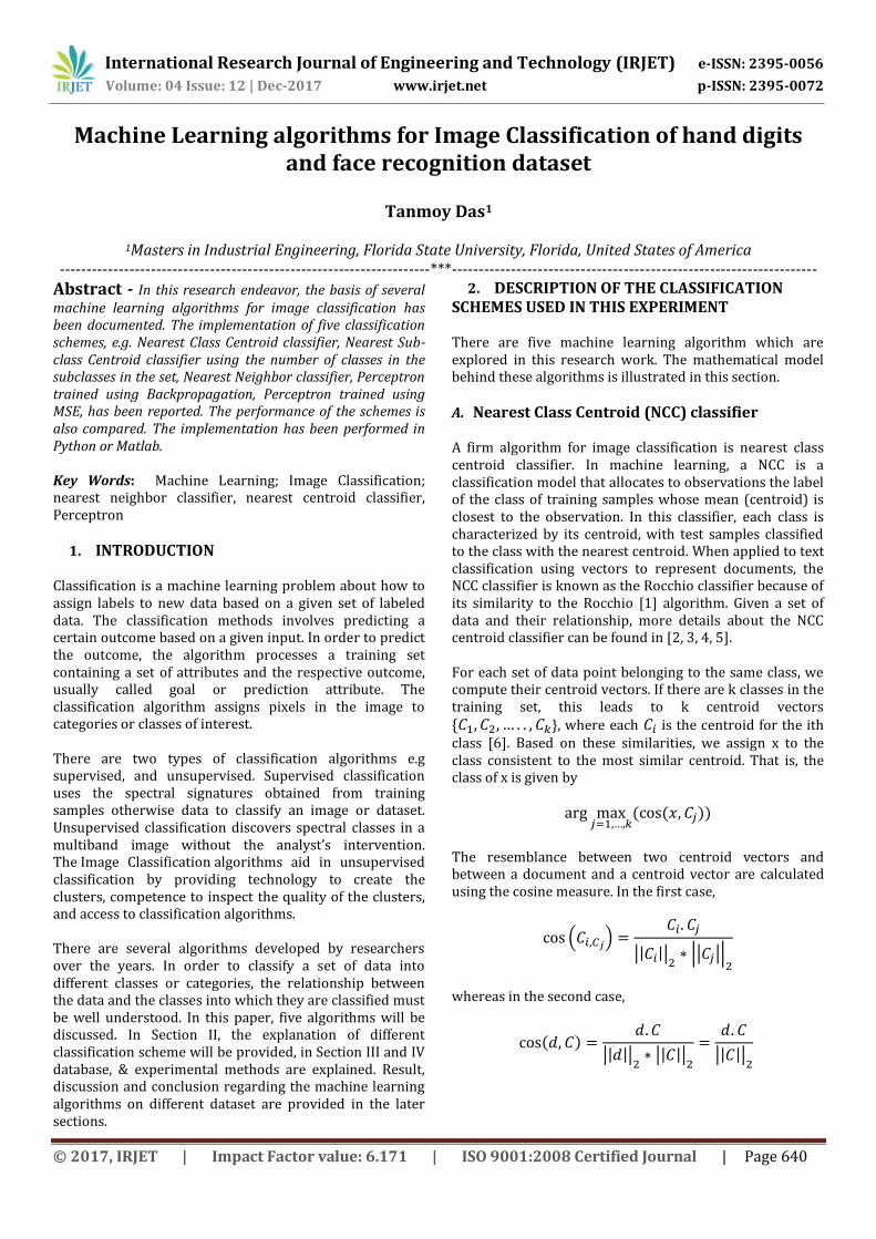
A graphic depiction of the nearest neighbor concept is illustrated in the Voronoi tessellation [12]. A Voronoi cell encapsulates all neighboring points that are nearest to each sample and is defined as

where is the Voronoi cell for sample , and x

represents all possible points within Voronoi cell . A graphical display of KNN is presented in Figure 1: KNN classification of data

Figure 1: KNN classification of data

D. Perceptron trained using Backpropagation Backpropagation is a technique utilized in artificial neural networks to calculate the error contribution of each neuron after a batch of data (in image recognition, multiple images) is processed. Backpropagation is an efficient method for computing gradients needed to perform gradient-based optimization of the weights in a multi-layer network. The Backpropagation algorithm is a supervised learning method for multilayer feed-forward networks from the field of Artificial Neural Networks (ANN). A neuron accepts input signals via its dendrites, which pass the electrical signal down to the cell body. The axon carries the signal out to synapses, which are the connections of a cell’s axon to other cell’s dendrites. The principle of the backpropagation approach is to model a given function by modifying internal weightings of input signals to produce an expected output signal. The system is trained using a supervised learning method, where the




error between the system’s output and a known expected output is presented to the system and used to modify its internal state. Technically, the backpropagation algorithm [13] is a

method for training the weights in a multilayer feed-

forward neural network. As such, it requires a network

structure to be well-defined of one or more layers where

one layer is fully coupled to the next layer. A standard

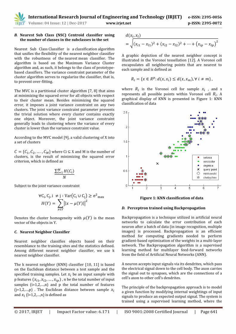
network structure is one input layer, one hidden layer, and

one output layer as shown in

Figure 2: Multilayer Neuron with Two hidden Layers.

Figure 2: Multilayer Neuron with Two hidden Layers

E. Perceptron trained using MSE Perceptrons are single layer binary classifier that splits the input spaces with a linear decision boundary. They are provide for historical interest.

Mean Squared Error,

where n is the number of instances in the data set This can be agreeable as it normalizes the error for data sets of different sizes. MSE is the average squared error per pattern. The MSE function would be obtained by the maximum likelihood (ML) principle assuming the independence and Gaussianity of the target data [14, 15]. The Mean Square Error maps all training data to arbitrary target values, meaning it finds the weight vector w that can meet the following

In matrix form,

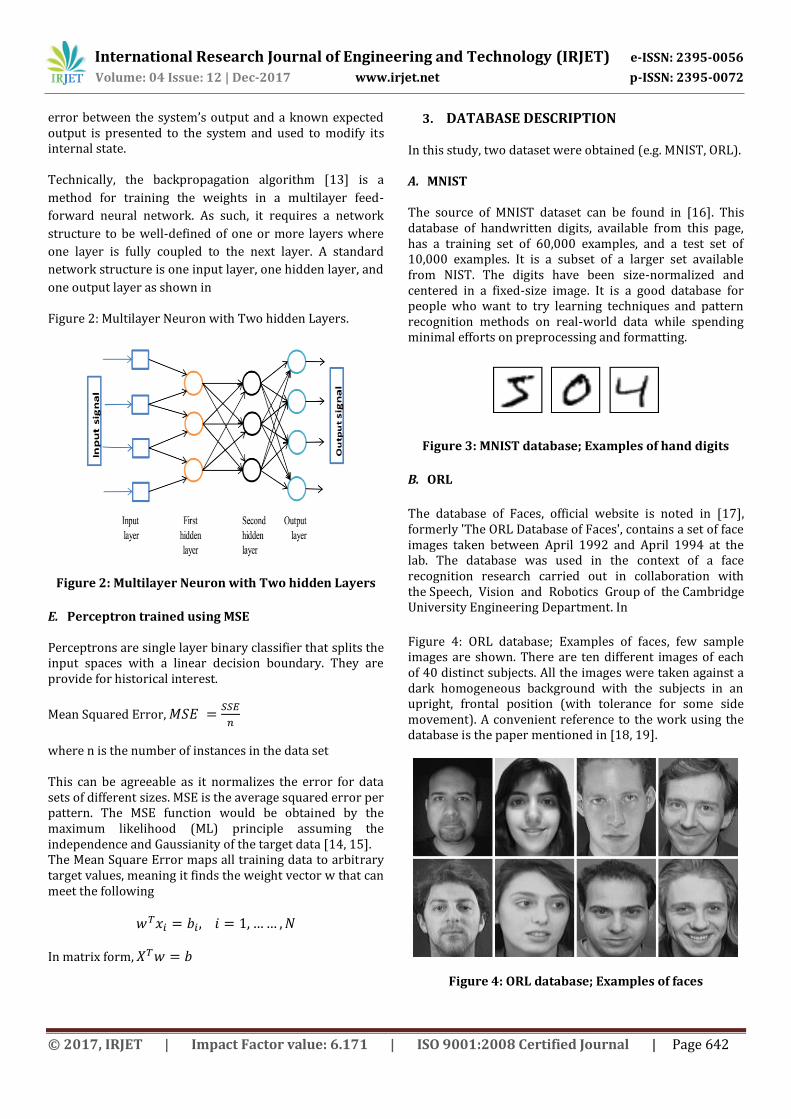
3. DATABASE DESCRIPTION In this study, two dataset were obtained (e.g. MNIST, ORL). A. MNIST The source of MNIST dataset can be found in [16]. This database of handwritten digits, available from this page, has a training set of 60,000 examples, and a test set of 10,000 examples. It is a subset of a larger set available from NIST. The digits have been size-normalized and centered in a fixed-size image. It is a good database for people who want to try learning techniques and pattern recognition methods on real-world data while spending minimal efforts on preprocessing and formatting.

Figure 3: MNIST database; Examples of hand digits

B. ORL

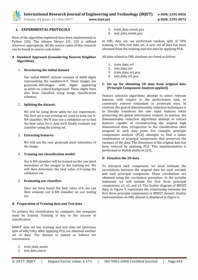
The database of Faces, official website is noted in [17], formerly 'The ORL Database of Faces', contains a set of face images taken between April 1992 and April 1994 at the lab. The database was used in the context of a face recognition research carried out in collaboration with the Speech, Vision and Robotics Group of the Cambridge University Engineering Department. In

Figure 4: ORL database; Examples of faces, few sample images are shown. There are ten different images of each of 40 distinct subjects. All the images were taken against a dark homogeneous background with the subjects in an upright, frontal position (with tolerance for some side movement). A convenient reference to the work using the database is the paper mentioned in [18, 19].

Figure 4: ORL database; Examples of faces

http://svr-www.eng.cam.ac.uk/

http://www.eng.cam.ac.uk/

http://www.eng.cam.ac.uk/




4. EXPERIMENTAL PROTOCOLS Most of the algorithm explained have been implemented in Python [20]. The sklearn library [21, 22] is utilized wherever appropriate. All the source codes of this research can be found in source code folder. A. Standard Approach (Considering Nearest Neighbor

Algorithm):

1. Structuring the initial dataset

Our initial MNIST dataset consists of 6000 digits representing the numbers 0-9. These images are grayscale, 8x8 images with digits appearing as white on a black background. These digits have also been classified using image classification schemes.

2. Splitting the dataset:

We will be using three splits for our experiment. The first set is our training set, used to train our k-NN classifier. We’ll also use a validation set to find the best value for k. And we’ll finally evaluate our classifier using the testing set.

3. Extracting features:

We will use the raw, grayscale pixel intensities of the image.

4. Training our classification model:

Our k-NN classifier will be trained on the raw pixel intensities of the images in the training set. We will then determine the best value of k using the validation set.

5. Evaluating our classifier:

Once we have found the best value of k, we can then evaluate our k-NN classifier on our testing set.

B. Preparation of Training data and Test data To achieve the classification by computer, the computer must be trained. Training is key to the success of classification MNIST data set has training and test data set (previous split of 60k/10k). After applying PCA, we obtained another set of data. The dataset is named as follows for convenience:

1. train_data_mnist 2. test_data_mnist

3. train_data_mnist_pca 4. test_data_mnist_pca

In ORL data set, we performed random split of 70% training vs 30% test data set. A new set of data has been obtained from the training and test data by applying PCA. All data related to ORL database are listed as follow:

1. train_data_orl 2. test_data_orl 3. train_data_orl_pca 4. test_data_orl_pca

C. Set up for obtaining 2D data from original date

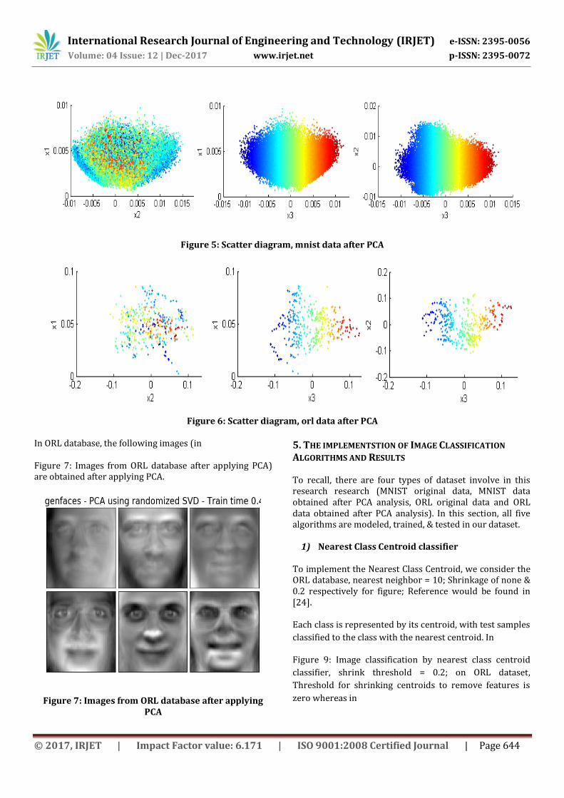
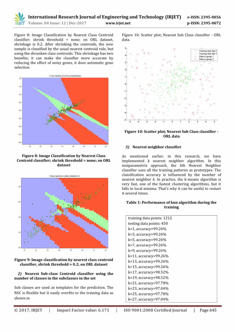
(Principle Component Analysis applied) Feature selection algorithms attempt to select relevant features with respect to the performance task, or conversely remove redundant or irrelevant ones. In contrast, the goal of dimensionality reduction techniques is to literally transform the raw input features while preserving the global information content. In essence, the dimensionality reduction algorithms attempt to extract features capable of reconstructing the original high dimensional data, irrespective to the classification label assigned to each data point. For example, principle components analysis (PCA) attempts to find a linear combination of principal components that preserves the variance of the data. The dimension of the original data has been reduced by applying PCA. This implementation is performed in Matlab platform [23]. D. Visualize the 2D data To interpret each component, we must estimate the correlations between the original data for each variable and each principal component. These correlations are obtained using the correlation procedure. In the variable statement we will include the first three principal components, x1, x2, and x3. The Scatter diagram of MNIST data, in Figure 5, represents the relationship between the first three principle components in MNIST dataset. Similar representation on ORL dataset is displayed in Figure 6.




Figure 5: Scatter diagram, mnist data after PCA

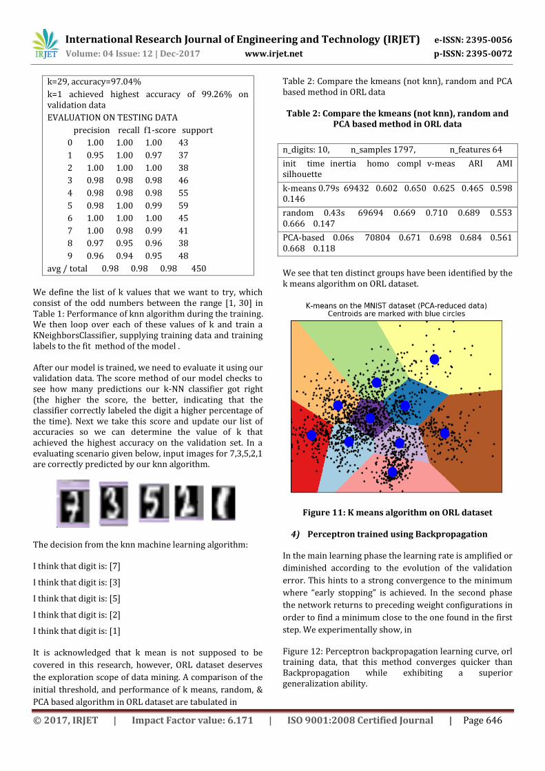
Figure 6: Scatter diagram, orl data after PCA In ORL database, the following images (in

Figure 7: Images from ORL database after applying PCA) are obtained after applying PCA.

Figure 7: Images from ORL database after applying PCA

5. THE IMPLEMENTSTION OF IMAGE CLASSIFICATION

ALGORITHMS AND RESULTS To recall, there are four types of dataset involve in this research research (MNIST original data, MNIST data obtained after PCA analysis, ORL original data and ORL data obtained after PCA analysis). In this section, all five algorithms are modeled, trained, & tested in our dataset.

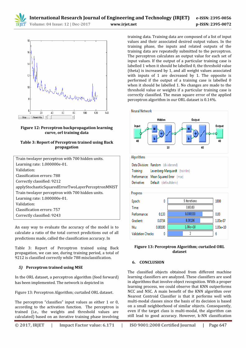
1) Nearest Class Centroid classifier To implement the Nearest Class Centroid, we consider the ORL database, nearest neighbor = 10; Shrinkage of none & 0.2 respectively for figure; Reference would be found in [24]. Each class is represented by its centroid, with test samples

classified to the class with the nearest centroid. In

Figure 9: Image classification by nearest class centroid

classifier, shrink threshold = 0.2; on ORL dataset,

Threshold for shrinking centroids to remove features is

zero whereas in



© 2017, IRJET | Impact Factor value: 6.171 | ISO 9001:2008 Certified Journal | 45

Figure 8: Image Classification by Nearest Class Centroid classifier; shrink threshold = none; on ORL dataset, shrinkage is 0.2. After shrinking the centroids, the new sample is classified by the usual nearest centroid rule, but using the shrunken class centroids. This shrinkage has two benefits; it can make the classifier more accurate by reducing the effect of noisy genes, it does automatic gene selection.

Figure 8: Image Classification by Nearest Class Centroid classifier; shrink threshold = none; on ORL

dataset

Figure 9: Image classification by nearest class centroid classifier, shrink threshold = 0.2; on ORL dataset

2) Nearest Sub-class Centroid classifier using the

number of classes in the subclasses in the set Sub classes are used as templates for the prediction. The

NSC is flexible but it easily overfits to the training data as

shown in

Figure 10: Scatter plot; Nearest Sub Class classifier - ORL data.

Figure 10: Scatter plot; Nearest Sub Class classifier - ORL data

3) Nearest neighbor classifier As mentioned earlier, in this research, we have implemented k nearest neighbor algorithm. In this nonparametrix approach, the kth Nearest Neighbor classifier uses all the training patterns as prototypes. The classification accuracy is influenced by the number of nearest neighbor k. In practice, the k-means algorithm is very fast, one of the fastest clustering algorithms, but it falls in local minima. That’s why it can be useful to restart it several times.

Table 1: Performance of knn algorithm during the training

training data points: 1212

testing data points: 450

k=1, accuracy=99.26%


















k=1 achieved highest accuracy of 99.26% on validation data

EVALUATION ON TESTING DATA

precision recall f1-score support

0 1.00 1.00 1.00 43

1 0.95 1.00 0.97 37

2 1.00 1.00 1.00 38

3 0.98 0.98 0.98 46

4 0.98 0.98 0.98 55

5 0.98 1.00 0.99 59

6 1.00 1.00 1.00 45

7 1.00 0.98 0.99 41

8 0.97 0.95 0.96 38

9 0.96 0.94 0.95 48

avg / total 0.98 0.98 0.98 450

We define the list of k values that we want to try, which consist of the odd numbers between the range [1, 30] in Table 1: Performance of knn algorithm during the training. We then loop over each of these values of k and train a KNeighborsClassifier, supplying training data and training labels to the fit method of the model . After our model is trained, we need to evaluate it using our validation data. The score method of our model checks to see how many predictions our k-NN classifier got right (the higher the score, the better, indicating that the classifier correctly labeled the digit a higher percentage of the time). Next we take this score and update our list of accuracies so we can determine the value of k that achieved the highest accuracy on the validation set. In a evaluating scenario given below, input images for 7,3,5,2,1 are correctly predicted by our knn algorithm.

The decision from the knn machine learning algorithm: I think that digit is: [7]

I think that digit is: [3]



I think that digit is: [1] It is acknowledged that k mean is not supposed to be

covered in this research, however, ORL dataset deserves

the exploration scope of data mining. A comparison of the

initial threshold, and performance of k means, random, &

PCA based algorithm in ORL dataset are tabulated in

Table 2: Compare the kmeans (not knn), random and PCA based method in ORL data

Table 2: Compare the kmeans (not knn), random and

PCA based method in ORL data

n_digits: 10, n_samples 1797, n_features 64

init time inertia homo compl v-meas ARI AMI silhouette

k-means 0.79s 69432 0.602 0.650 0.625 0.465 0.598 0.146

random 0.43s 69694 0.669 0.710 0.689 0.553 0.666 0.147

PCA-based 0.06s 70804 0.671 0.698 0.684 0.561 0.668 0.118

We see that ten distinct groups have been identified by the k means algorithm on ORL dataset.

Figure 11: K means algorithm on ORL dataset 4) Perceptron trained using Backpropagation

In the main learning phase the learning rate is amplified or

diminished according to the evolution of the validation

error. This hints to a strong convergence to the minimum

where “early stopping” is achieved. In the second phase

the network returns to preceding weight configurations in

order to find a minimum close to the one found in the first

step. We experimentally show, in

Figure 12: Perceptron backpropagation learning curve, orl training data, that this method converges quicker than Backpropagation while exhibiting a superior generalization ability.




Figure 12: Perceptron backpropagation learning curve, orl training data

Table 3: Report of Perceptron trained using Back

propagation

Train twolayer perceptron with 700 hidden units.

Learning rate: 1.000000e-01.

Validation:

Classification errors: 788

Correctly classified: 9212

applyStochasticSquaredErrorTwoLayerPerceptronMNIST

Train twolayer perceptron with 700 hidden units.

Learning rate: 1.000000e-01.

Validation:

Classification errors: 757

Correctly classified: 9243

An easy way to evaluate the accuracy of the model is to

calculate a ratio of the total correct predictions out of all

predictions made, called the classification accuracy. In

Table 3: Report of Perceptron trained using Back propagation, we can see, during training period, a total of 9212 is classified correctly while 788 misclassification.

5) Perceptron trained using MSE In the ORL dataset, a perceptron algorithm (feed forward)

has been implemented. The network is depicted in

Figure 13: Perceptron Algorithm; curtailed ORL dataset. The perceptron “classifies” input values as either 1 or 0, according to the activation function. The perceptron is trained (i.e., the weights and threshold values are calculated) based on an iterative training phase involving

training data. Training data are composed of a list of input values and their associated desired output values. In the training phase, the inputs and related outputs of the training data are repeatedly submitted to the perceptron. The perceptron calculates an output value for each set of input values. If the output of a particular training case is labelled 1 when it should be labelled 0, the threshold value (theta) is increased by 1, and all weight values associated with inputs of 1 are decreased by 1. The opposite is performed if the output of a training case is labelled 0 when it should be labelled 1. No changes are made to the threshold value or weights if a particular training case is correctly classified. The mean square error of the applied perceptron algorithm in our ORL dataset is 0.14%.

Figure 13: Perceptron Algorithm; curtailed ORL dataset

6. CONCLUSION The classified objects obtained from different machine learning classifiers are analyzed. These classifiers are used in algorithms that involve object recognition. With a proper learning process, we could observe that KNN outperforms NCC and NSC. A main benefit of the KNN algorithm over Nearest Centroid Classifier is that it performs well with multi-modal classes since the basis of its decision is based on a small neighborhood of similar objects. Consequently, even if the target class is multi-modal, the algorithm can still lead to good accuracy. However, k-NN classification




time was fairly long. Therefore, it performs that real time recognition is problematic. In contrast, the Back propagation method is long in learning time but is very short in recognition time. Exclusively if the number of dimensions of the samples is large, it can be believed that Backpropagation is better than k-NN in classification ability. The performance of various classification methods still depend, significantly, on the general characteristics of the data to be classified. The precise relationship between the data to be classified and the performance of various classification algorithms still remains to be revealed. Till date, there has been no classification method that works best on any given problem.

REFERENCES [1] Miao, Yun-Qian, and Mohamed Kamel. "Pairwise

optimized Rocchio algorithm for text categorization." Pattern Recognition Letters 32, no. 2 (2011): 375-382.

[2] Angiulli, Fabrizio. "Fast nearest neighbor

condensation for large data sets classification." IEEE Transactions on Knowledge and Data Engineering 19, no. 11 (2007).

[3] Tibshirani, Robert, Trevor Hastie,

Balasubramanian Narasimhan, and Gilbert Chu. "Diagnosis of multiple cancer types by shrunken centroids of gene expression." Proceedings of the National Academy of Sciences 99, no. 10 (2002): 6567-6572.

[4] G. Wilfong. Nearest neighbor problems. In

Proceedings of the seventh annual symposium on Computational geometry, pages 224–233. ACM Press, 1991

[5] Park, Haesun, Moongu Jeon, and J. Ben Rosen.

"Lower dimensional representation of text data based on centroids and least squares." BIT Numerical mathematics 43, no. 2 (2003): 427-448.

[6] Han, Eui-Hong Sam, and George Karypis.

"Centroid-based document classification: Analysis and experimental results." In European conference on principles of data mining and knowledge discovery, pp. 424-431. Springer, Berlin, Heidelberg, 2000.

[7] C.J. Veenman, M.J.T. Reinders, and E. Backer. A

maximum variance cluster algorithm. IEEE Transactions on Pattern Analysis and Machine Intelligence, 24(9):1273–1280, September 2002

[8] C.J. Veenman, M.J.T. Reinders, and E. Backer. A

cellular coevolutionary algorithm for image segmentation. IEEE Transactions on Image Processing, 12(3):304–316, March 2003.

[9] Veenman, Cor J., and Marcel JT Reinders. "The

nearest subclass classifier: A compromise between the nearest mean and nearest neighbor classifier." IEEE Transactions on Pattern Analysis and Machine Intelligence 27, no. 9 (2005): 1417-1429.

[10] Weinberger, Kilian Q., John Blitzer, and Lawrence

K. Saul. "Distance metric learning for large margin nearest neighbor classification." In Advances in neural information processing systems, pp. 1473-1480. 2006.

[11] Weinberger, Kilian Q., John Blitzer, and Lawrence

K. Saul. "Distance metric learning for large margin nearest neighbor classification." In Advances in neural information processing systems, pp. 1473-1480. 2006.

[12] Brandt, Jonathan W., and V. Ralph Algazi.

"Continuous skeleton computation by Voronoi diagram." CVGIP: Image understanding 55, no. 3 (1992): 329-338.

[13] Abdullah, Nabeel Ali, and Anas M. Quteishat.

"Wheat Seeds Classification using Multi-Layer Perceptron Artificial Neural Network." (2015): 306-309.

[14] Bishop, Christopher M. Neural networks for

pattern recognition. Oxford university press, 1995.

[15] Michalski, Ryszard S., Jaime G. Carbonell, and Tom

M. Mitchell, eds. Machine learning: An artificial intelligence approach. Springer Science & Business Media, 2013.

[16] LeCun, Y., Bottou, L., Bengio, Y., and Haffner, P.

(1998). Gradient-based learning applied to document recognition. Proceedings of the IEEE, 86, 2278–2324.

[17] Cl.cam.ac.uk. (2017). The Database of Faces.

[online] Available at: http://www.cl.cam.ac.uk/research/dtg/attarchive/facedatabase.html [Accessed 23 Nov. 2017].

[18] Samaria, Ferdinando S., and Andy C. Harter.

"Parameterisation of a stochastic model for human face identification." In Applications of Computer Vision, 1994., Proceedings of the

http://www.pymvpa.org/references.html#lbb-98

http://www.pymvpa.org/references.html#lbb-98




Second IEEE Workshop on, pp. 138-142. IEEE, 1994.

[19] Zabaras, Nicholas. "Principal Component

Analysis."(2014). [20] Jones E, Oliphant E, Peterson P, et al. SciPy: Open

Source Scientific Tools for Python, 2001-, http://www.scipy.org/ [Online; accessed 2017-11-26].

[21] Scikit-learn: Machine Learning in Python,

Pedregosa et al., JMLR 12, pp. 2825-2830, 2011. [22] Pedregosa, Fabian, Gaël Varoquaux, Alexandre

Gramfort, Vincent Michel, Bertrand Thirion, Olivier Grisel, Mathieu Blondel et al. "Scikit-learn: Machine learning in Python." Journal of Machine Learning Research 12, no. Oct (2011): 2825-2830.

[23] MATLAB 2014a, The MathWorks, Natick, 2014

Scikit-learn.org. (2017).

[24] sklearn.neighbors.NearestCentroid — scikit-learn 0.19.1 documentation. [online] Available at: http://scikit-learn.org/stable/modules/generated/sklearn.neighbors.NearestCentroid.html

machine learning algorithms for image classification of ... · machine learning algorithms for...

Documents