Machine Learning and Deep LearningAlgorithms for Bearing Fault Diagnostics

– A Comprehensive ReviewShen Zhang∗†, Shibo Zhang‡, Bingnan Wang∗, and Thomas G. Habetler†

∗Mitsubishi Electric Research Laboratories, 201 Broadway, Cambridge, MA 02139, USA†School of Electrical and Computer Engineering, Georgia Institute of Technology, Atlanta, GA 30332, USA

‡Computer Science, Northwestern University, Evanston, IL 60201, USA

Abstract—In this survey paper, we systematically summarizethe current literature on studies that apply machine learning(ML) and data mining techniques to bearing fault diagnostics.Conventional ML methods, including artificial neural network(ANN), principal component analysis (PCA), support vectormachines (SVM), etc., have been successfully applied to detectingand categorizing bearing faults since the last decade, while theapplication of deep learning (DL) methods has sparked greatinterest in both the industry and academia in the last five years.In this paper, we will first review the conventional ML methods,before taking a deep dive into the latest developments in DL algo-rithms for bearing fault applications. Specifically, the superiorityof the DL based methods over the conventional ML methodsare analyzed in terms of metrics directly related to fault featureextraction and classifier performances; the new functionalitiesoffered by DL techniques that cannot be accomplished before arealso summarized. In addition, to obtain a more intuitive insight, acomparative study is performed on the classifier performance andaccuracy for a number of papers utilizing the open source CaseWestern Reserve University (CWRU) bearing data set. Finally,based on the nature of the time-series 1-D data obtained fromsensors monitoring the bearing conditions, recommendations andsuggestions are provided to applying DL algorithms on bearingfault diagnostics based on specific applications, as well as futureresearch directions to further improve its performance.

Index Terms—Bearing fault; diagnostics; machine learning;deep learning; feature extraction

I. INTRODUCTION

Electric machines are widely employed in a variety ofindustry application processes and electrified transportationsystems. However, for certain applications these machines mayoperate under unfavorable conditions, such as high ambienttemperature, high moisture and overload, which can eventuallyresult in motor malfunctions that lead to high maintenancecosts, severe financial losses, and safety concerns [1]–[3]. Themalfunction of electric machines can be generally attributed tovarious faults of different categories, which include the driveinverter failures, stator winding insulation breakdown, as wellas bearing faults and air gap eccentricity. Several surveys re-garding the likelihood of induction machine failures conductedby the IEEE Industry Application Society (IEEE-IAS) [4]–[6]and the Japan Electrical Manufacturers’ Association (JEMA)[7] reveal that a bearing fault is the most common fault typethat accounts for 30% to 40 % percent of the total faults.

Since a bearing is the most vulnerable component in a motorand drive system, bearing fault detection has been a researchfrontier for engineers and scientists for the past decades.Specifically, this problem is approached by interpreting avariety of available signals, including vibration [10], [11],acoustic noise [12], [13], stator current [14], [15], thermal-imaging [16], and multiple sensor fusion [17]. The existenceof a bearing fault as well as its specific fault type can bereadily determined by performing frequency spectral analysison the monitored signals and analyzing the components at thecharacteristic fault frequencies, which can be calculated by awell-defined mechanical model [8] that depends on the motorspeed, the bearing geometry and the specific location of adefect inside the bearing.

However, accurately identifying the occurrence of a bearingfault can be sometimes difficult in practice, especially whenthe fault is still at its incipient stage due to the small signal-to-noise ratio of the vibration and acoustic signals. In addition,unlike other motor failures (stator inter-turn, broken rotor bar,etc. [3]) that can be accurately determined by the electric sig-nals, the uniqueness of bearing failures lies in its multi-physicsnature, incorporating a closed-loop interplay between theinitiative mechanical vibration and the corresponding inducedharmonics in the electric signals, which further affects theoutput torque , motor speed, and finally the vibration patternitself. As a result, the accuracy of the traditional mathematicalmodel-based bearing fault diagnostics can be further influ-enced by background noise due to external mechanical excitedmotion, while its sensitivity is also subject to change based onsensor mounting positions and spatial constraints in a highly-compact design. Therefore, a popular alternative approach forbearing fault detection is accomplished by analyzing the statorcurrent [14], [15], which is measured in most motor drivesand thus would not bring extra device or installation costs.Despite its advantages such as economic savings and simpleimplementation, stator current signature analysis can encountermany practical issues. For example, the magnitude of statorcurrents at bearing fault signature frequencies can vary atdifferent loads, different speeds, and different power ratingsof the motors themselves, thus bringing challenges to identifythe threshold stator current values to trigger a fault alarm atan arbitrary operating condition. Therefore, a thorough and

1

arX

iv:1

901.

0824

7v1

[cs

.LG

] 2

4 Ja

n 20

19

systematic testing is usually required while the motor is still atthe healthy condition, and the healthy data would be collectedwhile the targeted motor is running at different load andspeed. This process, summarized as a “Learning Stage” inpatent US5726905 [18], is unfortunately tedious and expensiveto perform, and needs to be repeated for any motor with adifferent power rating.

Most of the challenges described above can be attributedto the fact that all the conventional methods rely solely uponthe values at the fault characteristic frequencies to determinethe presence of a bearing fault. However, there may existsome unique patterns or relationships hidden in the datathemselves that can potentially reveal a bearing fault, andthese special features can be almost impossible for humans toidentify at the first place. Therefore, many researchers beganapplying various machine learning algorithms, i.e., artificialneural networks (ANN), principal component analysis (PCA),support vector machines (SVM), etc., to better parse the data,learn from them, and then apply what they’ve learned to makeintelligent decisions regarding the presence of bearing faults[30]–[33]. Most of the literature applying these ML algorithmsreport very satisfactory results with classification accuracyover 90%.

To achieve even better performance and higher classificationaccuracy under versatile operating conditions or noisy condi-tions, deep learning based methods are becoming increasinglypopular to meet this need. This literature survey incorporatesaround 160 papers, around 60 of which employed some typeof deep learning based approaches. And the number of papersgrows steadily, with 2 papers published in 2015, 7 papersin 2016, 17 papers in 2017 and 37 papers in 2018, clearlyindicating booming interests in employing DL methods forbearing fault diagnostics in the recent years. Deep learninggenerally requires extremely large datasets, and some DLnetworks in computer vision were trained using as manyas 1.2 million images. For many applications, including thediagnostics of bearing faults, such large datasets are not readilyavailable and will be expensive and time consuming to acquire.For smaller datasets, classical ML algorithms can competewith or even outperform deep learning networks.

In this context, this paper seeks to present a thoroughoverview on the recent research work devoted to applying ma-chine learning techniques on bearing fault diagnostics. The restof the paper is organized as below. In Section II, we introducesome of the most popular datasets used for bearing fault detec-tion. Next, in Section III, we look into traditional ML methods,including ANN, PCA, k-nearest neighbors (k-NN), SVM, etc.,with a brief explanation of each method. For the main part ofthe paper, in Section IV, we take a deep dive into the researchfrontier of identifying a bearing fault with DL techniques. Inthis part, we will provide our understanding of the researchtrend toward DL networks. The advantages of the DL basedmethods over the conventional ML methods will be analyzedin terms of metrics directly related to fault feature extractionand classifier performances; the new functionalists offered byDL techniques that cannot be accomplished before are also

Fig. 1. Experimental setup collecting the CWRU bearing dataset [26].

summarized. We will also give detailed analysis to each ofmajor DL techniques, including convolutional neural network(CNN), auto-encoder, deep belief network (DBN), recurrentneural network (RNN), generative adversarial network (GAN),and their applications to bearing fault detection. In SectionV, to obtain a more intuitive insight, a comparative study isperformed on the different DL algorithms, as well as theirclassifier performances utilizing the common open source CaseWestern Reserve University (CWRU) bearing data set. Finally,based on the nature of the time-series 1-D data obtained fromsensors monitoring the bearing conditions, recommendationsand suggestions on applying DL algorithms for bearing faultdiagnostics for specific applications are provided in sectionVI, as well as future research directions to further improve itsperformance by adopting more complex datasets and predictthe actual bearing fault with classifiers trained with artificiallyinduced faults.

II. POPULAR BEARING FAULT DATASETS

Data is the foundation for all machine learning and artifi-cial intelligence methods. To develop effective ML and DLalgorithms for bearing fault detection, a good collection ofdatasets is necessary. Since the bearing degradation processmay take many years, most people conduct experiment andcollect data either using bearings with artificially injectedfaults, or with accelerated life testing method. While thedata collection is still time consuming, fortunately a feworganizations have made the effort and provided bearing faultdatasets for people to work on the ML research. These datasetsalso serve as standards for the evaluation and comparison ofdifferent algorithms.

Before getting into the details of various ML developments,in this section, we briefly introduce a few popular datasets usedby most papers covered in this review.

A. Case Western Reserve University (CWRU) Dataset

The test stand used to acquire the Case Western ReserveUniversity (CWRU) bearing dataset is illustrated in Fig. 1, inwhich a 2 hp induction motor is shown on the left, a torquetransducer/encoder is in the middle, while a dynamometer iscoupled on the right. Single point faults were introduced to

2

Y. Chen et al. / Neurocomputing 294 (2018) 61–71 65

Fig. 5. Difference between standard convolution and atrous convolution.

and γ l ( i ) and β l ( i ) are the scale and shift parameters to be learned,

respectively.

2.4. Auxiliary classifiers

As stated in [24] , the features produced by the hidden lay-

ers of a well-performed inception net are very discriminative. Fur-

thermore, the auxiliary classifiers corresponding to these hidden

inception layers act as some kind of a regularizer [28] and also

improve the convergence behavior [29] . The effect of auxiliary clas-

sifiers has been proved in many experiments with inception net,

such as [30] .

Generally, the goal of training a CNN model is to determine the

optimal weights of kernels and biases in each layer so that the

CNN model could have the minimum classification error. Combin-

ing all layers of weights gives:

W M

=

(W

( 1 ) , . . . , W

( M ) )

(4)

where W

( i ) is the weight of i th layer, and M is the number of lay-

ers. Analogously, the corresponding weights of an auxiliary classi-

fier with the m th layer can be denoted by:

W m

=

(W

( 1 ) , . . . , W

( m ) )

(5)

Therefore, the total objective function is:

F ( W ) ≡ P ( W M

) + Q ( W m

) (6)

in which the output objective is P( W M

) ≡‖ w

(out) ‖ 2 + �( W M

, w

(out) ) ,

the auxiliary objective is Q( W m

) ≡ α[ ‖ w

(m ) ‖ 2 + �( W m

, w

(m ) ) ] , and

the classifier weights for the i th layer are denoted as w

( i ) .

Note that w

( m ) depends on W m

. By adding the auxiliary objec-

tive, the overall goal of producing a good classification of output

does not change and the auxiliary part acts as a type of regulariza-

tion or as a proxy for discriminative features.

In our paper, auxiliary classifiers play a similar but more impor-

tant role in our model. With respect to the difficulties in discover-

ing the common features between data generated from artificial

damaged bearings and data generated from natural damaged bear-

ings, we suggest using the ensemble learning algorithm with the

classification of different classifiers based on different scale fea-

tures. This is where the auxiliary classifiers come in. In ACDIN,

two auxiliary classifiers with softmax as the activation function are

constructed. The first auxiliary classifier based on the second stage

of the inception layers is used to increase the training gradient,

while the second one based on the fourth stage of the inception

layers is used to stabilize the terminal classification result. All clas-

sifiers (including the auxiliary ones and the final one) deliver the

classification results as vectors with each element corresponding

to the possibility of each type. Since the outputs of the classifiers

are in the same shape, their summary is the terminal classification

result of ACDIN. Moreover, in our experiment, these two auxiliary

classifiers stabilize the loss of validation data and improve conver-

gence during training, and also make some contributions to the ac-

curacy of the test data.

3. Validation of the proposed ACDIN model

In the real world, data from natural damaged bearings is rare,

while data from artificial damaged bearings can be easily collected.

However, distinctions between these two kinds of data always con-

fuse many classification algorithms. From the results of the follow-

ing experiments, ACDIN shows its better performance in address-

ing this problem, compared to traditional learning machines and

CNN models. Then, more experiments have been conducted to an-

alyze ACDIN.

3.1. Data description

The dataset we used to verify the proposed model comes from

the Chair of Design and Drive Technology, Paderborn University.

This dataset is collected from a modular test rig as shown in Fig. 6 .

The test rig consists or several modules: an electric motor (1) , a

torque-measurement shaft (2) , a rolling bearing test module (3) , a

flywheel (4) and a load motor (5) . A more detailed description can

be found in [21] .

In this dataset, the vibration signals of bearings running in the

test rig are measured and saved with a sampling rate of 64 kHz.

Bearings are run at a rotational speed of 1500 rpm with a load

torque of 0.1 Nm and a radial force on the bearing of 10 0 0 N.

There are three possible statuses of bearings: healthy, inner race

fault and outer race fault. These faults are either caused by artifi-

cial methods or natural operation.

The detailed situation of healthy bearings, artificial damaged

bearings and natural damaged bearings are shown in Tables 1–3 . In

Fig. 6. Modular Test Rig.

Fig. 2. Modular test rig collecting the Paderborn bearing dataset consistingof (1) an electric motor, (2) a torque-measurement shaft, (3) a rolling bearingtest module, (4) a flywheel and (5) a load motor [27].652 IEEE TRANSACTIONS ON INDUSTRIAL ELECTRONICS, VOL. 62, NO. 1, JANUARY 2015

Fig. 5. CNC machine [Singapore Institute of Manufacturing Technology (SIMTECH Institute)] and PRONOSTIA testbed (Department of AutomaticControl and Micro-Mechatronic Systems (AS2M), Franche-Comté Electronique Mécanique Thermique et Optique-Sciences et Technologies(FEMTO-ST) Institute). (a) CNC machine, work piece, and sensors. (b) PRONOSTIA bearing testbed.

TABLE IIKEY FEATURES OF THE PHM CHALLENGE DATA SETS FROM TWO APPLICATIONS

learning scheme is synthesized in Fig. 4. Details can be foundin [34].

IV. EXPERIMENTS, RESULTS, AND DISCUSSION

A. PHM Challenge Data Sets

To demonstrate the effectiveness of our contributions, weconsider the vibration data from two real applications underconstant operating conditions: 1) cutting tools from a computernumerical control (CNC) machine [39] [see Fig. 5(a)]; and2) ball bearings from the experimental platform PRONOSTIA[25], [40] [see Fig. 5(b)]. Key features of both applications aresummarized in Table II, and a brief introduction is given asfollows.

• Cutting tools are used for an extremely dynamical cut-ting process. The in situ monitoring during the cuttingprocess can give important information about the toolcondition, the process itself, the work-piece surface qual-ity, and even the machine condition [4]. CM systemsfor the cutting process are normally based on the mea-surements of vibration, acoustic emission, and cuttingforce. However, the vibration measurement benefits from awide frequency range, less restrictive conditions, and easyimplementation [41].

• Bearings are of great importance because rotating machin-ery often includes bearing inspections and replacements,which implies high maintenance costs. However, it is hardto evaluate the model performance due to the inherentnonlinearity in features extracted from raw vibration data[3], [42]. In this context, the platform PRONOSTIA isdedicated to test and validate the fault detection, diagno-sis, and prognostics methods on ball bearings. It allows

performing accelerated degradations of bearings by con-stant and/or variable operating conditions while gatheringCM data (load force, speed, vibration, and temperature).

B. Feature Extraction and Selection Results

As aforementioned in Section III-B1, the decomposition ofthe vibration signal requires the selection of a mother waveletand a decomposition level. Therefore, as suggested in literature,for the cutting-tool application, a Daubechies wavelet of thefourth order (db4) [26] and the third [43] level of decompositionwere used, whereas for the bearings, db4 and the fourth levelwere considered [27], prior to feature extraction.

1) Classical Features Versus Trigonometric Features:Here, we compare the performance of trigonometric featureswith that of classical features on cutter C1 (from the CNC ma-chine) and bearing Ber1−1 (from PRONOSTIA) (see Fig. 6(a)and (c), respectively). For both cases, the vibration data ap-pear to be noisy with low trendability. In particular, for bear-ing Ber1−1, the vibration signal is almost constant until thefourth hour, but it suddenly grows at the end. The results inFig. 6(a) and (c) show that the classical features from both cases(C1 and Ber1−1) have low monotonicity/trendability and highnoise/scales. Therefore, consider now the proposition of featureextraction using a combination of the SD and trigonometricfunctions (see Table I). The results in Fig. 6(b) and (d) showthat the trigonometric features clearly reflect failure progressionwith high monotonicity and trendability and have lower scalesas compared with the classical features.

Back to the accuracy of prognostics, one can point outthat classical features (RMS, Kurtosis, etc.) are not welladapted to catch machine conditions. Moreover, they can havelarge scales, which require normalization before feeding a

Fig. 3. PRONOSTIA testbed (Department of Automatic Control and Micro-Mechatronic Systems (AS2M), Franche-Comte Electronique Mecanique [29].

the test bearings using electro-discharge machining with faultdiameters of 7 mils, 14 mils, 21 mils, 28 mils, and 40 mils, atthe inner raceway, rolling element and outer raceway. Vibrationdata was collected for motor loads of 0 to 3 horsepower andmotor speeds of 1797 to 1720 rpm using two accelerometersinstalled at both the drive end and fan end of the motorhousing, and two sampling frequencies of 12 kHz and 48kHz were used. The generated dataset was recorded and madepublicly available on the CWRU bearing data center website[26].

The CWRU dataset serves as a fundamental dataset tovalidate the performance of different ML algorithms, and acomprehensive comparative study on all prior work employingthe CWRU dataset will be presented in section V.

B. Paderborn University Dataset

The Paderborn university bearing dataset [27] includes thesynchronously measured motor currents and vibration signals,thus enabling the verification of multi-physics models, aswell as the cross-validation and fusion of different signalsto increase bearing fault diagnostic accuracy. Both the statorcurrent and vibration signals are measured with high resolutionand sampling rate, and experiments were performed on 26damaged bearing states and 6 undamaged (healthy) states forreference. Among the damaged bearings, 12 were artificiallydamaged, and the other 14 were with real damages caused byaccelerated life tests. This enables more accurate testing andimplementation of the ML algorithms in practical applications,where the real defects are generated through aging and thegradual lost of lubrication. The modular test rig to acquire thePaderborn bearing dataset is illustrated in Fig. 2.

C. PRONOSTIA Dataset

Another popular dataset for predicting bearing’s remaininguseful life (RUL) is known as “PRONOSTIA bearings ac-celerated life test dataset”, which serves as the fundamentaldataset for researchers investigating new algorithms on bearingRUL prediction. The main objective of PRONOSTIA is toprovide real data related to accelerated degradation of bearingsperformed under constant and/or variable operating conditions,which are online controlled.

The operating conditions are characterized by two sensors:a rotating speed sensor and a force sensor. In PRONOSTIAplatform as shown in Fig. 3, the bearings health monitoringis ensured by gathering two types of signals: temperatureand vibration (with horizontal and vertical accelerometers).Furthermore, the data are recorded with a specific samplingfrequency which allows the catching of the whole frequencyspectrum of the bearing during its degradation process. Ul-timately, the monitoring data provided by the sensors can beused for further processing in order to extract relevant featuresand continuously assess the health condition of the bearing.

During the International Conference on Prognostics andHealth Management (PHM), a “IEEE PHM 2012 PrognosticChallenge” was organized. For this purpose, a web link tothe degradation data [28] is provided to the competitors toallow them testing and verifying their prognostic methods.The results of each method can then be evaluated regardingits capability to accurately estimate the RUL of the testedbearings.

D. Summary

So far a majority of papers on bearing fault identificationwith ML algorithms employ the CWRU dataset for its sim-plicity and popularity. The authors anticipate a growing trendof interests will emerge on the Paderborn dataset as it containsboth the stator current signal and the vibration signal. Besides,many researchers working on RUL prediction also use thePRONOSTIA dataset. Since the main scope of this paper ison bearing fault identification, research contributions on RULprediction is not included in this literature survey.

III. TRADITIONAL MACHINE LEARNING BASEDAPPROACHES

The structure of a rolling-element bearing is illustrated inFig. 4, which contains the outer race typically mounted on themotor cap, the inner race to hold the motor shaft, the ballsor rolling elements, and the cage for restraining the relativedistances of the rolling elements. The four common scenariosof misalignment that are likely to cause bearing failures aredemonstrated in Fig. 4(a) to (d).

Before ML actually goes deep, there are a variety of clas-sical “shallow” machine learning and data mining algorithmsthat have been around for many years, i.e., the artificial neuralnetworks (ANN) based on back-propagation. Applying thesealgorithms requires a lot of domain expertise and complexfeature engineering, since a deep exploratory data analysis is

3

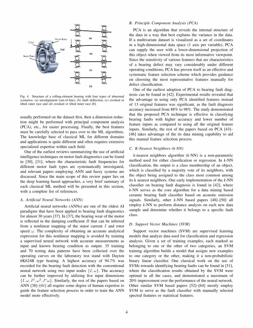
Fig. 4. Structure of a rolling-element bearing with four types of abnormalscenarios: (a) misalignment (out-of-line), (b) shaft deflection, (c) crooked ortilted outer race and (d) crooked or tilted inner race [8].

usually performed on the dataset first, then a dimension reduc-tion might be performed with principal component analysis(PCA), etc., for easier processing. Finally, the best featuresmust be carefully selected to pass over to the ML algorithms.The knowledge base of classical ML for different domainsand applications is quite different and often requires extensivespecialized expertise within each field.

One of the earliest reviews summarizing the use of artificialintelligence techniques on motor fault diagnostics can be foundin [30], [31], where the characteristic fault frequencies fordifferent motor fault types are systematically investigated,and relevant papers employing ANN and fuzzy systems arediscussed. Since the main scope of this review paper lies onthe deep learning based approaches, a very brief summary ofeach classical ML method will be presented in this section,with a complete list of references.

A. Artificial Neural Networks (ANN)

Artificial neural networks (ANNs) are one of the oldest AIparadigms that have been applied to bearing fault diagnosticsfor almost 30 years [37]. In [37], the bearing wear of the motoris reflected in the damping coefficient B that can be inferredfrom a nonlinear mapping of the stator current I and rotorspeed ω. The complexity of obtaining an accurate analyticalexpression for this nonlinear mapping is avoided by traininga supervised neural network with accurate measurements asinput and known bearing condition as output. 35 trainingand 70 testing data patterns have been collected over theoperating curves on the laboratory test stand with Dayton6K624B type bearing. A highest accuracy of 94.7% wasrecorded for the bearing fault detection with the conventionalneural network using two input nodes {I, ω}. The accuracycan be further improved by utilizing five input dimensions{I, ω, I2, ω2, I∗ω}. Similarly, the rest of the papers based onANN [38]–[41] all require some degree of human expertise toguide the feature selection process in order to train the ANNmodel more effectively.

B. Principle Component Analysis (PCA)

PCA is an algorithm that reveals the internal structure ofthe data in a way that best explains the variance in the data.If a multivariate dataset is visualized as a set of coordinatesin a high-dimensional data space (1 axis per variable), PCAcan supply the user with a lower-dimensional projection ofthis object when viewed from its most informative viewpoint.Since the sensitivity of various features that are characteristicsof a bearing defect may vary considerably under differentoperating conditions, PCA has proven itself as an effective andsystematic feature selection scheme which provides guidanceon choosing the most representative features manually fordefect classification.

One of the earliest adoption of PCA to bearing fault diag-nosis can be found in [42]. Experimental results revealed thatthe advantage in using only PCA identified features insteadof 13 original features was significant, as the fault diagnosisaccuracy increased from 88% to 98%. The study demonstratedthat the proposed PCA technique is effective in classifyingbearing faults with higher accuracy and lower number offeature inputs as compared to using all the original featureinputs. Similarly, the rest of the papers based on PCA [43]–[46] takes advantage of the its data mining capability to aidthis manual feature selection process.

C. K-Nearest Neighbors (k-NN)

k-nearest neighbors algorithm (k-NN) is a non-parametricmethod used for either classification or regression. In k-NNclassification, the output is a class membership of an object,which is classified by a majority vote of its neighbors, withthe object being assigned to the class most common amongits k nearest neighbors. One early implementation of the k-NNclassifier on bearing fault diagnosis is found in [42], wherek-NN serves as the core algorithm for a data mining basedceramic bearing fault classifier based on acoustic emissionsignals. Similarly, other k-NN based papers [48]–[50] allemploy k-NN to perform distance analysis on each new datasample and determine whether it belongs to a specific faultclass.

D. Support Vector Machines (SVM)

Support vector machines (SVM) are supervised learningmodels that analyze data used for classification and regressionanalysis. Given a set of training examples, each marked asbelonging to one or the other of two categories, an SVMtraining algorithm builds a model that assigns new examplesto one category or the other, making it a non-probabilisticbinary linear classifier. One classical work on the use ofSVMs towards identifying bearing faults can be found in [51],where the classification results obtained by the SVM wereoptimal in all the cases, and demonstrated a maximum of20% improvement over the performance of the neural network.Other similar SVM based papers [52]–[64] mostly employSVM to serve as the fault classifier with manually selectedspectral features or statistical features.

4

Fig. 5. Performance comparison of deep learning and most other learningalgorithms [103].

E. Others

Besides the commonly used ML methods listed above,many other algorithms with different characteristics have beenapplied to the identification of bearing faults, including theneural fuzzy network [65]–[67], Bayesian networks [68]–[70],self-organizing maps [71], [72], extreme learning machines(ELM) [73], [74], transfer learning [76]–[78], discriminateanalysis [79]–[81], random forest [82], independent compo-nent analysis [83], Softmax classifiers [84], manifold learning[85], [86], canonical variate analysis [87], particle filter [88],nonlinear preserving projection [89], artificial HydrocarbonNetworks [90], class imbalanced learning (CIL), ensemblelearning (EL), multi-scale permutation entropy (MPE) [93],empirical mode decomposition [94]–[98], topic correlationanalysis [99], affinity propagation [100], and dictionary learn-ing [101], [102].

IV. APPLICATION OF DEEP LEARNING BASEDAPPROACHES

Deep learning is a subset of machine learning that achievesgreat power and flexibility by learning to represent the worldas nested hierarchy of concepts, with each concept defined inrelation to simpler concepts, and more abstract representationscomputed in terms of less abstract ones. The trend of transi-tioning from traditional shallow ML methods to deep learningcan be attributed to the following reasons.

1) Hardware evolution: Training deep networks is extremelycomputationally intensive, but running on a high per-formance GPU can significantly accelerate this trainingprocess. Specifically, the GPUs offer parallel computingcapability and computational compatibility with deepneural network, which makes them indispensable fortraining DL based algorithms. More powerful GPUsallows data scientists to quickly get the deep learningtraining up and running. For example, the NVIDIA TeslaV100 Tensor Core GPUs [104] can now parse petabytesof data orders of magnitude faster than traditional CPUs,and leverage mixed precision to accelerate deep learningtraining throughputs across every type of neural network.In most recent years, the emerging of different DL

computing platforms such as FPGA, ASIC, and TPU(Tensor Processing Units) as well as high performanceGPUs for embedded system expedites the fast evolutionof deep learning algorithms.

2) Algorithm evolution: More techniques and frameworksare invented and getting matured in terms of controllingthe training process of deeper models to achieve fasterspeed, better convergence, and better generalization. Forexample, algorithms such as RELU that helps accelerateconvergence speed; techniques that prevent overfittingsuch as dropout and pooling. The development of nu-merical optimization also provides the horsepower ofleveraging more data and training deeper models, suchas mini-batch Gradient Descent, RMSprop, and L-BFGSoptimizer.

3) Data explosion: With the availability of more sensorsinstalled that collect an increasing amount of data, and theapplication of crowdsourced labeling mechanism such asAmazon mTurk [105], we have seen a surging appearanceof large scale dataset in many domains, such as ImageNetin image recognition, MPI Sintel Flow in image opticalflow, VoxCeleb in speaker identification, et al. The perfor-mance of deep learning can significantly outperform mosttraditional ML algorithms, especially with the increaseof dataset dimension, as illustrated in Fig. 5 [103] byAndrew Ng.

All of the factors above contribute to the new era ofapplying deep learning algorithms to a variety of data-relatedapplications. Specifically, the advantages of applying deeplearning algorithms compared to traditional ML algorithmsinclude:

1) Best-in-class performance: The complexity of the com-puted function grows exponentially with depth [106].Deep learning has best-in-class performance that sig-nificantly outperforms other solutions on problems inmultiple domains, including speech, language, vision,playing games like Go, etc.

2) Automatic feature extraction: No need for feature en-gineering. Traditional machine learning algorithms usu-ally call for sophisticated manual feature engineeringwhich unavoidably involves expert domain knowledgeand numerous human effort. However, when using a deepnetwork, there’s no need for this; as one can just passthe data directly to the network and usually achieve goodperformance right off the bat. This totally eliminates thechallenging feature engineering stage.

3) Transferability: The strong expressive power and highperformance of a deep neural network trained in onedomain can be easily generalized or transferred to othercontexts or settings. Deep learning is an architecturethat can be adapted to new problems relatively eas-ily. For instance, problems in vision, time series, andlanguage are using same techniques like convolutionalneural networks, recurrent neural networks, long short-term memory etc.

5

Thanks to the above reasons for the transition from MLmethods to DL methods, as well as the explicit benefits ofthe DL algorithms discussed above, we have witnessed anexponential increase in deep learning applications. One suchexample is the fault diagnostics and health prognostics, andbearing fault identification is a very representative case.

A. Convolutional Neural Network (CNN)

Inspired by animal visual cortex [107], convolution opera-tion is first introduced to detect image patterns in a hierarchicalway from simple features, such as edge and corner, to complexfeatures. The low layers detect fundamental low level visualfeatures such as edge and corner; and the layers afterwarddetect higher level features, which are built upon simple lowlevel features.

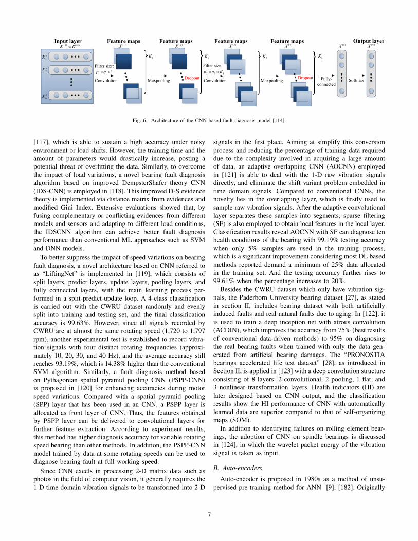
The first paper employing CNN to identify bearing faultwas published in 2016 [108] and for the next three yearsmany papers [109]–[112], [114]–[124] emerged on this topicthat contributed to its performance advancement in variousaspects. The basic architecture of a CNN-based bearing faultclassifier is illustrated in Fig. 6. The 1-D temporal raw dataobtained from different accelerometers are firstly stacked toa 2-D matrix form, similar to the representation of images,which is then passed through a convolution layer for featureextraction, followed by a pooling layer for down-sampling.The combination of this convolution-pooling can be repeatedmany times to further deepen the network. Finally, the outputfrom the hidden layers will be passed along to one or severalfully-connected (FC) layers, the result of which serves as theinput to a top classifier such as Softmax or Sigmoid functions.

In [108], the vibration data were acquired using two ac-celerometers installed on the x- and y- directions, one on topof the housing, and the other on the back of the housing.CNN is able to autonomously learn useful features for bearingfault detection from the raw data pre-processed by the scaledDFT transform. The classification results demonstrate thatthe feature-learning based approach significantly outperformsthe feature-engineering based approach based on conventionalML methods. Moreover, the authors have shown that feature-learning based approaches such as CNN can also performbearing health prognostics, and identify some early-stagefaulty conditions without explicit characteristic frequencies,such as lubrication degradation, which cannot be identified bytraditional ML methods.

An adaptive CNN (ADCNN) is applied on the CWRUdataset to dynamically change the learning rate, for a bet-ter trade-off between training speed and accuracy in [109].The entire fault diagnosis model employs of a fault patterndetermination component using 1 ADCNN and a fault sizeevaluation component using 3 ADCNNs, 3-layer CNNs withmax pooling. Classification results on the test set demonstrateADCNN has a better accuracy compared to conventionalshallow CNN and SVM methods, especially in terms ofidentifying the rolling element (ball) defect. In addition, thisproposed ADCNN is also able to predict the fault size (defect

width) with satisfactory accuracy. On top of the conventionalstructure of CNN, a dislocate layer is added in [110] that canbetter extract the relationship between signals with differentintervals in periodic forms, especially during the change ofoperating conditions. The best accuracy of 96.32% is achievedwith a disclose step factor k = 3, while the accuracy ofconventional CNN without this disclose layer is only 83.39%.Similar to earlier work [108]–[110], [111] implements a 4-layer CNN structure with 2 convolutional and 2 pooling layersemploying both the CWRU dataset & dataset generated byQian Peng Company in China, and the accuracy outperformsthe conventional SVM and shallow Softmax regression clas-sifier, especially when the vibration signal is mixed withambient noise, this improvement can be as large as 25%,showcasing the excellent built-in denoising capabilities of theCNN algorithm itself. A sensor fusion approach is applied in[112], in which both temporal and spatial information of theCWRU raw data from the two accelerometers at both the driveend and fan end are stacked by transforming 1-D time-seriesdata into 2-D input matrix and sent to CNN as input. 70%of the samples are used for training, 15% for validation, and15% for testing; average accuracy with two sensors is 99.41%,while the accuracy with only one sensor is 98.35%.

Many variations of CNN are also employed to tackle thebearing fault diagnosis challenge [114]–[121] on the CWRUdataset to obtain more desirable characteristics comparedto the conventional CNN. For example, a CNN based onLeNet-5 [113] is applied in [114] containing 2 alternatingconvolutional-pooling layers and a 2 fully-connected (FC)layers. Padding is used to control the size of learned features,and zero-padding is applied to prevent dimension loss. Thisimproved CNN architecture is believed to provide better fea-ture extraction capability, as the accuracy on the test set is anastonishing 99.79%, which is better than other deep learningbased methods such as the adaptive CNN (98.1%) and deepbelief network (87.45%), and dominates the traditional MLmethods such as SVM (87.45%) and ANN (67.70%). In addi-tion, a deep fully CNN (DFCNN) incorporating 4 convolution-pooling layer pairs is employed in [115], while the raw data arealso transformed into spectrograms for easier processing. Anaccuracy of 99.22% is accomplished, outperforming 94.28% ofthe linear SVM with particle swarm optimization (PSO), and91.43% of the conventional SVM. These percentage numbersare obtained by the same authors, using the same training andtest set to train the conventional ML algorithms that serve asbenchmark cases. To save the extensive training time requiredfor most CNN based algorithms, a multi-scale deep CNN(MS-DCNN) is adopted in [116], where convolution kernelof different sizes are used to extract different-scale featuresin parallel. The mean accuracy of 9-layer 1d-CNN, 2d-CNNand the proposed MS-DCNN are 98.57%, 98.25% and 99.27%,respectively. Despite the subtle increase in accuracy comparedto conventional CNNs, the number of parameters to be deter-mined via training is only 52,172, significantly fewer than 1-DCNN (171,606) and 2-D CNN (213,206). Moreover, a verydeep CNN of 14 layers with training interference is used in

6

104 IEEE/ASME TRANSACTIONS ON MECHATRONICS, VOL. 23, NO. 1, FEBRUARY 2018

Fig. 2. Architecture of the CNN-based fault diagnosis model.

and complicated object models in latter layers. The classificationlayer can use the learned bank of filters (or the extracted features)to achieve the classification.

III. CNN-BASED FAULT DIAGNOSIS WITH

MULTIPLE SENSORS

This paper proposes an intelligent fault diagnosis approachfor rotating machinery based on CNN with the raw data frommultiple sensors. With the appealing capability of automaticfeature extraction of the approach, no hand-crafted features areneeded to classify different conditions. Multiple sensor fusion atdata level is achieved by combining the raw data from multiplesensors into a 2-D matrix at the input layer. Fig. 1 shows theflowchart of the proposed fault diagnosis method. Conditionmonitoring data of the running machinery is collected frommultiple sensors such as vibration signals from accelerometers.After denoising and preprocessing, these sets of 1-D time seriesare stacked row by row to form a 2-D input matrix. The temporalinformation and the spatial information from the sensors areconstructed in the input matrix in this manner. All the collectedsamples are then divided into training, validation, and testingdataset. The training dataset is used to train the initialized CNNmodel by minimizing the error between the predicted conditionand the actual one. The validation dataset is used to select amodel before possible overfitting. The generalization capabilityof the trained model is then evaluated by the testing dataset. Nomanual feature extraction or selection is needed in this approachas the representative features are automatically extracted duringthe training process.

Fig. 2 shows the detailed structure of the CNN-based faultdiagnosis model. Machine condition monitoring data Xn

i , (i =1, 2, . . . ,m) from m vibration sensors is collected and fusedat the data level as input X ∈ Rm×n of the CNN model. Theinput is convolved by K1 filters of size p1 × q1 × 1. The ReLUoperation is applied on the convolved outcome to form the K1

feature maps with dimension (m − p1 + 1) × (n − q1 + 1). Amax-pooling layer is followed to subsample the feature maps byusing (4). Followed by another such stage, the convolution pro-cess aims to capture the representative features from the inputdata. A fully connected layer and a softmax layer are added nextto output the machine condition. Minibatch stochastic gradientdescent is used in this paper to update the parameters of themodel in the training process using (6) through (8). After train-ing, the CNN model extracts representative features directlyfrom the raw vibration signals from multiple sensors. Fault di-agnosis can then be performed on new monitoring data.

Fig. 3. Experimental setup of the CWRU dataset.

Overfitting is a common issue in training, which leads toa poor performance on the test data especially with limitedtraining data. This paper uses dropout to prevent overfitting.Dropout is a technique that avoids extracting same featuresrepeatedly to reduce the chance of overfitting [36]. During eachiteration of training, neurons are randomly dropped out, whichmeans temporarily removed from the network, along with alltheir incoming and outgoing connections with probability p,so that a reduced network is left for training [37]. It can beimplemented by setting the selected elements of the featuremaps to zero. In the testing phase, the dropout is turned OFF

and the probability p will be multiplied by each feature mapelement. Dropout is considered to exponentially combine manydifferent neural network architectures in an efficient way to findthe fittest model.

IV. EXPERIMENTAL EVALUATION

To evaluate the effectiveness of the proposed approach for ro-tating machinery fault diagnosis, two typical rotating machinery,bearings and gearboxes, are investigated in this paper. Vibrationsignals of different machine conditions are collected throughmultiple accelerometers.

A. Case One: Bearing Fault Diagnosis

1) Experimental Setup and Data Description: In thiscase study, the public available roller bearing condition datasetcollected from a motor drive system by Case Western ReserveUniversity (CWRU) is analyzed [38]. The objective is todiagnose the different faults of bearing also with different levelsof severity. The main components of the experimental setup

Fig. 6. Architecture of the CNN-based fault diagnosis model [114].

[117], which is able to sustain a high accuracy under noisyenvironment or load shifts. However, the training time and theamount of parameters would drastically increase, posting apotential threat of overfitting the data. Similarly, to overcomethe impact of load variations, a novel bearing fault diagnosisalgorithm based on improved DempsterShafer theory CNN(IDS-CNN) is employed in [118]. This improved D-S evidencetheory is implemented via distance matrix from evidences andmodified Gini Index. Extensive evaluations showed that, byfusing complementary or conflicting evidences from differentmodels and sensors and adapting to different load conditions,the IDSCNN algorithm can achieve better fault diagnosisperformance than conventional ML approaches such as SVMand DNN models.

To better suppress the impact of speed variations on bearingfault diagnosis, a novel architecture based on CNN referred toas “LiftingNet” is implemented in [119], which consists ofsplit layers, predict layers, update layers, pooling layers, andfully connected layers, with the main learning process per-formed in a split-predict-update loop. A 4-class classificationis carried out with the CWRU dataset randomly and evenlysplit into training and testing set, and the final classificationaccuracy is 99.63%. However, since all signals recorded byCWRU are at almost the same rotating speed (1,720 to 1,797rpm), another experimental test is established to record vibra-tion signals with four distinct rotating frequencies (approxi-mately 10, 20, 30, and 40 Hz), and the average accuracy stillreaches 93.19%, which is 14.38% higher than the conventionalSVM algorithm. Similarly, a fault diagnosis method basedon Pythagorean spatial pyramid pooling CNN (PSPP-CNN)is proposed in [120] for enhancing accuracies during motorspeed variations. Compared with a spatial pyramid pooling(SPP) layer that has been used in an CNN, a PSPP layer isallocated as front layer of CNN. Thus, the features obtainedby PSPP layer can be delivered to convolutional layers forfurther feature extraction. According to experiment results,this method has higher diagnosis accuracy for variable rotatingspeed bearing than other methods. In addition, the PSPP-CNNmodel trained by data at some rotating speeds can be used todiagnose bearing fault at full working speed.

Since CNN excels in processing 2-D matrix data such asphotos in the field of computer vision, it generally requires the1-D time domain vibration signals to be transformed into 2-D

signals in the first place. Aiming at simplify this conversionprocess and reducing the percentage of training data requireddue to the complexity involved in acquiring a large amountof data, an adaptive overlapping CNN (AOCNN) employedin [121] is able to deal with the 1-D raw vibration signalsdirectly, and eliminate the shift variant problem embedded intime domain signals. Compared to conventional CNNs, thenovelty lies in the overlapping layer, which is firstly used tosample raw vibration signals. After the adaptive convolutionallayer separates these samples into segments, sparse filtering(SF) is also employed to obtain local features in the local layer.Classification results reveal AOCNN with SF can diagnose tenhealth conditions of the bearing with 99.19% testing accuracywhen only 5% samples are used in the training process,which is a significant improvement considering most DL basedmethods reported demand a minimum of 25% data allocatedin the training set. And the testing accuracy further rises to99.61% when the percentage increases to 20%.

Besides the CWRU dataset which only have vibration sig-nals, the Paderborn University bearing dataset [27], as statedin section II, includes bearing dataset with both artificiallyinduced faults and real natural faults due to aging. In [122], itis used to train a deep inception net with atrous convolution(ACDIN), which improves the accuracy from 75% (best resultsof conventional data-driven methods) to 95% on diagnosingthe real bearing faults when trained with only the data gen-erated from artificial bearing damages. The “PRONOSTIAbearings accelerated life test dataset” [28], as introduced inSection II, is applied in [123] with a deep convolution structureconsisting of 8 layers: 2 convolutional, 2 pooling, 1 flat, and3 nonlinear transformation layers. Health indicators (HI) arelater designed based on CNN output, and the classificationresults show the HI performance of CNN with automaticallylearned data are superior compared to that of self-organizingmaps (SOM).

In addition to identifying failures on rolling element bear-ings, the adoption of CNN on spindle bearings is discussedin [124], in which the wavelet packet energy of the vibrationsignal is taken as input.

B. Auto-encoders

Auto-encoder is proposed in 1980s as a method of unsu-pervised pre-training method for ANN [9], [182]. Originally

7

relationships in machinery fault diagnosis issues [14–16]. Consequently, it is necessary to design deep architectures forrotating machinery fault diagnosis.

Deep learning is a new unsupervised feature learning method with multiple hidden layers of representation [17]. Thegreatest advantage of deep learning is that the features of each hidden layer are not designed manually, which is, theyare learned from the input data automatically [18]. Despite it is not surprising that deep learning has produced extremelysatisfactory results for various tasks, it is still in its infancy for machinery fault diagnosis. Tamilselvan et al. applied deeplearning for aircraft engine fault diagnosis [19]. Tran et al. used deep learning for reciprocating compressor valves fault diag-nosis [20]. Shao et al. proposed optimization deep learning model for rolling bearing fault diagnosis [21]. However, there stillexists manual signal processing or feature selection in these methods, in other words, they treated the deep learning modelsas traditional classifiers, which ignored the powerful ability of deep learning in automatically capture the useful informationfrom the raw vibration signals.

Deep autoencoder is a popular deep learning model, which has been successfully used in various applications [22]. Due toits simplicity and efficiency, the mean square error (MSE) has been widely applied to design the deep autoencoder loss func-tion [23]. Standard deep autoencoder under MSE usually performs very well when the signals are not disturbed by complexnoises. However, in most practical situations, the measured vibration signals are always affected by the variable operatingconditions and heavy background noises, which make the performance of the standard deep autoencoder deteriorate rapidly[24,25]. Therefore, the research and development of the new deep autoencoder loss function has become an urgent task.

In this paper, a novel deep autoencoder feature learning method is proposed for rotating machinery fault diagnosis. Theproposed method is applied for the fault diagnosis of gearbox and electrical locomotive roller bearings. The results show thatthe proposed method is more effective and robust than other methods. The main contributions of our work can be summa-rized as follows.

(1) In order to get rid of the dependence on signal processing techniques and diagnosis experience, we propose a deepautoencoder feature learning method to automatically and effectively learn the useful fault features from the mea-sured vibration signals.

(2) In order to eliminate the background noise affection and enhance the feature learning ability, maximum correntropy isused to design the new deep autoencoder loss function.

(3) In order to enable the deep autoencoder to adapt to the signal characteristics, artificial fish swarm algorithm (AFSA) isadopted to optimize its key parameters.

The organization of the paper is as follows. In Section 2, the basic theory of autoencoder is briefly introduced. The pro-posed method is described in Section 3. In Section 4, the experimental diagnosis results for gearbox are analyzed and dis-cussed. The engineering application of the proposed method is presented in Section 5. Finally, general conclusions aregiven in Section 6.

2. The basic theory of autoencoder

An autoencoder is a three-layer network including an encoder and a decoder, shown in Fig. 1. The encoder maps the inputdata from a high-dimensional space into codes in a low-dimensional space, and the decoder reconstructs the input data fromthe corresponding codes [26].

x1

x2

x3

xD

h1

h2

hd

z1

z2

z3

zD

Encoder Decoder

Dix

dih

Diz

Fig. 1. The structure of an autoencoder.

188 H. Shao et al. /Mechanical Systems and Signal Processing 95 (2017) 187–204

Fig. 7. Process of training a one hidden layer auto-encoder [129].

it was not called with the same terminology we are usingtoday. After evolving for decades, auto-encoder has becomewidely adopted as an unsupervised feature learning methodand a greedy layer-wise neural network pre-training method.

The training process of a one hidden layer auto-encoder isillustrated in Fig. 7. An auto-encoder is trained from an ANN,which composes of two parts: encoder and decoder. The outputof encoder is fed into the decoder as input. The ANN takesthe mean square error between the original input and outputas loss function, which essentially aims at imitating the inputas the final output. After this ANN is trained, the decoder partis dropped and only the encoder part is kept. Therefore theoutput of the encoder is the feature representation that can beemployed in next-stage classifiers.

There are many studies employing auto-encoder in bearingfault diagnosis [125]–[138]. One of the earliest can be foundin [125], where a 5-layer auto-encoder based DNN is utilizedto mine fault characteristics from the frequency spectrumadaptively for various diagnosis issues, and effectively classifythe health conditions of the machinery. The classificationaccuracy reaches 99.6%, which is significantly higher thanthe 70% of back-propagation based neural networks (BPNN).In [126], an auto-encoder based extreme learning machine(ELM) is employed seeking to integrate the automatic featureextraction capability of auto-encoders and the high trainingspeed of ELMs. The average accuracy of 99.83% comparesfavorably against other traditional ML methods, includingwavelet package decomposition based SVM (WPD-SVM)(94.17%), EMD-SVM (82.83%), WPD-ELM (86.75%) andEMD-ELM (81.55%). More importantly, the required trainingtime drops by around 60% to 70% using the same trainingand test data, thanks to the adoption of ELM.

Compared to CNN, the denoising capabilities of originalauto-encoders is not prominent. Thus in [127], a stacked de-noising autoencoder (SDA) is implemented, which is suitablefor deep architecture-based robust feature extraction on signalscontaining ambient noise and working condition fluctuations.This specific SDA consists of three auto-encoders stackedtogether. To balance between performance and training speeds,three hidden layers with 100, 50, and 25 units respectively

are employed. The original CWRU bearing data are perturbedby a 15dB random noise to mimic the noisy condition, andmultiple operating condition datasets are used as test setsto examine its fault identification capability under speed andload changes. This method achieves a worst case accuracy of91.79%, which is 3% to 10% higher compared to conventionalSAE without denoising capability, SVM and random forest(RF) algorithms. Similar to [127], another form of SDA isutilized in [128] with three hidden layers of (500, 500, 500)units, signals of the CWRU dataset are combined with differentlevels of artificially random noises in the time domain andlater converted to frequency signals. The proposed method hasbetter diagnosis accuracy than deep belief networks (DBN),particularly with the added noises, where an improvement of7% in fault diagnosis accuracy is achieved.

Besides the most commonly used CWRU dataset, vibrationdata collected from an electrical locomotive bearing test rig,developed at the Northwestern Polytechnical University ofChina, is used to validate the performance of auto-encoders.Based on this dataset, the authors in [129] adopted themaximum correntropy as the loss function instead of thetraditional mean square error, and one of swarm intelligencealgorithms called artificial fish-swarm algorithm (AFSA) isused to optimize the key parameters in the loss function ofauto-encoder. Results show that the customized 5-layer auto-encoder composed of maximum correntropy loss functionand AFSA algorithm outperforms a standard auto-encoderby an accuracy of 10% to 40% on the test set in a 5-classclassification problem. Similarly, a new deep AE constructedwith DAE and contractive auto-encoder (CAE) is applied tothe locomotive bearing dataset for the enhancement of featurelearning ability. A DAE is first used to learn the low-layerfeatures from the raw vibration data, then multiple CAEs areused to learn the deep features based on the learned low-layerfeatures. In addition, locality preserving projection (LPP) isalso adopted to fuse the deep features to further improve thequality of the learned features. The classification accuracy ofthe proposed DAE-CAE-LPP approach is 91.90%, showcasingan advantage over standard DAE (84.60%), standard CAE(85.10%), BPNN(49.70%) and SVM (57.60%). However, allautoencoder based methods are also 6 to 10 times more time-consuming compared to conventional BPNN and SVM.

In addition. an aircraft-engine inter-shaft bearing vibrationdataset with inner race, outer race and rolling element defectsis adopted as the input data in [131], where a new AEbased on Gaussian radial basis kernel function is employedto enhance the feature learning capability. Later, a stacked AEwas developed with this new AE and multiple conventionalAEs with an accuracy of 86.75%, which is much better com-pared to standard SAE (44.90%) and standard DBN (19.65%).Moreover, the importance of the proposed Gaussian radialbasis kernel function was presented: if the kernel functionis changed to either a polynomial kernel function (PK) or apower exponent kernel function (PEK), the accuracy woulddrop to 24.25% and 65.55%, respectively.

Similar to the case of CNN, many variations of SAE are

8

also employed to tackle the bearing fault diagnosis challenge[132]–[138] on the CWRU dataset to achieve better perfor-mance compared to the traditional SAE. An ensemble deepauto-encoders (EDAE) is employed in [132] with a seriesof auto-encoders (AE) with different activation functions forunsupervised feature learning from the measured vibrationsignals. Later a combination strategy is designed to ensureaccurate and stable diagnosis results. The classification accu-racy is 99.15%, which shows performance boosts comparedto BPNN (88.22%), SVM (90.81%), and RF (92.07%), afterperforming a 24-dimension manual feature extraction process.Similarly, by altering the activation function, a deep waveletauto-encoder (DWAE) with extreme learning machine (ELM)is implemented in [133], where the wavelet function is em-ployed as the nonlinear activation function to design waveletauto-encoders (WAE) to effectively capture the signal charac-teristics. Then a DWAE with multiple WAEs is constructed toenhance the unsupervised feature learning ability, and ELM isadopted as the output classifier. The input data dimension is,and the output accuracy achieves 95.20%. According to [133],this method not only outperforms conventional ML methodssuch as BPNN (85.43%) and SVM (87.97%), but also somestandard deep learning algorithms, including the standard DAE+ soft-max (89.70%) and standard DAE + ELM (89.93%).

Considering the relatively large dataset required to traindeep neural nets, a 4-layer DNN with stacked sparse au-toencoder (SSAE) is established in [134] with a compressionratio of 70%, indicating only 30% of the original data areneeded to train the proposed model. The DNN has 720 inputnodes, 200 and 60 nodes in the first and second hiddenlayer, and 7 nodes in the output layer (dependent on thenumber of fault conditions in a dataset). A nonlinear projectionis performed to compress the vibration data and automaticadaptive feature extraction in the transform domain; accuracycan reach 97.47%, which is 8% better than SVM, 60%better than a three-layer ANN and 46% better than multi-layer ANNs. In [135], two limitations of conventional SAEare summarized. The first one is that SAE tends to extractsimilar/redundant features that increases the complexity ratherthan accuracy of the model. Secondly, the learned featuresmay have shift variant properties. To overcome these issues, anew SAE-LCN (local connection network) is proposed, whichconsists of the input layer, local layer, feature layer and outputlayer. Specifically, this method first uses SAE to locally learnfeatures from input signals in the local layer, then obtains shift-invariant features in the feature layer, and finally recognizesmechanical health conditions in the output layer for a 10-classes problem. The average accuracy is 99.92%, which is 1%to 5% higher than many EMD, ensemble NN, and DL basedmethods. Similarly, the fault data are utilized to automaticallyextract the representative features by means of SAE in [136],while the diagnosis model is constructed by using ISVM. Thismodel has been also tested for online diagnosis purposes.

Besides the most commonly used Softmax classifiers inthe output layer, the Gath-Geva (GG) clustering algorithm isimplemented in [137], which induces a fuzzy maximum like-

1696 IEEE TRANSACTIONS ON INSTRUMENTATION AND MEASUREMENT, VOL. 66, NO. 7, JULY 2017

Fig. 4. Architecture of DBN.

all the feature sets were divided into two groups, one fortraining and the other for testing. Secondly, SAE was appliedfor feature fusion. Finally, the fused features were input intothe DBN for fault classification.

The feature fusion and classification of our proposed methodincludes the following six procedures.

1) Data Segmentation: The vibration data were obtainedfrom multiple accelerometers mounted on different loca-tions under different running conditions, and then weresegmented for grouping into two categories, one fortraining and the other for testing.

2) Feature Extraction: All the time-domain and frequency-domain features were extracted from each data set.

3) Normalization: All the feature vectors were normalizedand rescaled into range [0, 1], according to

x(i) = x(i) − x(i)min

x(i)max − x(i)

min

(8)

4) Initialization: Initializing the AE parameters W and brandomly, and setting up maximum epochs, learning rateand sparsity parameter.

5) Feature Fusion: Two-layer SAEs were trained throughminimizing the reconstruction error and the output ofthe last hidden layer was regarded as the fault featurerepresentations.

6) DBN Classification: The fused features were utilizedto train the DBN based classification model, and thenthe testing data sets were used to validate the proposedSAE-DBN method.

C. Deep Belief Network

DBN composed of multiple layers of RBMs can be effi-ciently trained in an unsupervised, layer-by-layer manner.Lower layers of DBN can extract low-level features in agreedy way and the upper layers are used to represent moreabstract characteristics of the input data. In this paper, DBNis composed by stacking three layers of RBMs, as shownin Fig. 4. Each RBM is a two-layer energy-based model with

Fig. 5. Restricted Boltzmann machine.

visible units and hidden units. Connections only exist betweenthe visible units of the input layer and the hidden units of thehidden layer.

The DBN learning process includes two stages: in the firststage, pretraining the RBM layer step by step in a greedyway, and in the second stage, fine-tuning the whole networkto adjust the parameters for achieving an ideal performance.The training data were firstly input into the visible vector fortraining the first RBM in an unsupervised manner. And thenthe feature representations produced by the level below wereregarded as the input to train the next RBM. This trainingprocess was repeated until the last RBM was learnt.

RBM is a special case of Boltzmann machines and Markovrandom fields as shown in Fig. 5. There are a number ofneurons in every RBM layer, which are independent of eachother. A neuron with only inactivated and activated states canbe represented in binary value 0 and 1, respectively. Supposinga RBM consists of visible vector v and hidden vector h,the joint probability distribution of (v, h) is given by the energyfunction

E(v, h, θ ) = −m∑

j=1

b j v j −n∑

i=1

ci hi −n∑

i=1

m∑

j=1

v j wi, j hi (9)

where w,b,c are the model parameters, v j and h j are the binarystates of visible unit j and hidden unit i , b j and ci are theirbiases, respectively, and wi, j is the weight between visibleunit j and hidden unit i .

The joint distribution over the visible and hidden units isdefined as follows:

p(v, h; θ) = 1

Z(θ)exp(−E(v, h; θ)) (10)

where the partition function Z(θ) = ∑v,h exp(−E(v, h)).

Because there are no visible-visible or hidden-hidden con-nections, the conditional probabilities over hidden and visibleunits are given by

p(hi = 1|v; θ) = 1/

⎡⎣1 + exp

⎡⎣−ci −

m∑

j=1

v j wi, j

⎤⎦

⎤⎦

(11)

p(v j = 1|h; θ) = 1/

[1 + exp

[−b j −

n∑

i=1

hi wi, j

]]

(12)

To train the DBN model, a fast algorithm so-called con-trastive divergence, was proposed by Hinton et al. [22]. First,the conditional probability of hidden units can be obtained byusing (11), then Gibbs sampling is employed to determine the

Fig. 8. Architecture of DBN [140].

lihood estimation (FMLE) of the distance norm to determinethe degree of a sample belonging to each cluster. While an8-layer SDAE is still used to extract the useful features andreduces the dimension of the vibration signal, GathGeva isdeployed to identify the different fault types. The worst caseclassification accuracy is 93.3%, outperforming the traditionalEMD based feature extraction schemes by almost 10%.

To reduce DL based model complexity, another bearing faultdiagnosis method based on fully-connected winner-take-allautoencoder is proposed in [138], in which the model explicitlyimposes lifetime sparsity on the encoded features by keepingonly k% largest activations of each neuron across all samplesin a mini-batch. A soft voting method is implemented to ag-gregate prediction results of signal segments sliced by a slidingwindow to increase accuracy and stability. A simulated datasetis generated by adding white Gaussian noise to original signalsof the CWRU dataset to test the diagnosis performance undernoisy environment. The experimental results demonstrate thatwith a simple two-layer network, the proposed method is notonly capable of diagnosing with high precision under normalconditions, but also has better robustness to noise than somedeeper and more complex models, such as CNN.

C. Deep Belief Network (DBN)

In deep learning, a Deep Belief Network (DBN) can beviewed as a composition of simple, unsupervised networkssuch as Restricted Boltzmann Machines (RBMs) or autoen-coders, where each sub-network’s hidden layer serves as thevisible layer for the next, as illustrated by the boxes ofdifferent colors in Fig. 8. An RBM is an undirected, generativeenergy-based model with a “visible” input layer, a hiddenlayer, and connections in between, but not within layers.This composition leads to a fast, layer-by-layer unsupervisedtraining procedure, where contrastive divergence is applied toeach sub-network in turn, starting from the “lowest” pair oflayers (the lowest visible layer in a training set).

9

H Jiang et al

3

where fh and fo are the activation functions of the hidden layer and the output layer, respectively, Wih are the weight matrix connecting input layer with a hidden layer, Whh is the weight matrix of the hidden layer to its own loop connection, Who is the connection weight matrix between the hidden layer and the output layer, and bh and bo are bias vectors of the hidden layer and output layer, respectively.

However, a conventional RNN as shown in figure  1 has inherent flaws. According to figure 1(b), we can see that the architecture of the RNN across time steps is equivalent to an FNN with multiple hidden layers, and the number of time steps can be regarded as its total number of layers. When the RNN is trained using back propagation through time (BPTT), the error back propagates not only from the output layer to the hidden layer but also through time t to time 1 simultaneously [38]. However, it can be seen that if t is too large, the learning process will be especially challenging due to the gradient van-ishing or the exploding problem [36].

Therefore, an improved RNN model, named the long-short term memory recurrent neural network (LSTMRNN), was proposed to overcome the flaws of the conventional RNN [39]. From figure 2, we can see that the LSTMRNN can be acquired by replacing the hidden neurons of a conventional RNN with long-short term memory (LSTM) units. The most obvious characteristic of an LSTM unit is that it mainly consists of a memory cell and three layer gates, i.e. an input gate, forget gate, and output gate. In addition, the dashed lines connecting the memory cell with three layer gates are called peephole connections [40]. Such architecture of the LSTM cell greatly relaxes the problem of gradient vanishing or exploding. Therefore, this paper adopts the LSTMRNN model to get sat-isfactory results. The mathematical calculation procedure of an LSTM unit can be described as

gt = g (Wih · xt + Whh · ht−1 + bh) , (3)

it = σ(Wiig · xt + Whig · ht−1 + pig � ct−1 + big

), (4)

ft = σ(Wifg · xt + Whfg · ht−1 + pfg � ct−1 + bfg

), (5)

ot = σ(Wiog · xt + Whog · ht−1 + pog � ct + bog

), (6)

ct = it � gt + ft � ct−1, (7)

ht = ot � h (ct) , (8)

where σ, g, and h are the gate activation function, the input, and the output activation functions of the LSTM units, respec-tively; Wih, Wiig, Wifg, and Wiog are the weight matrices between the input layer and the LSTM layer at time t; Whh, Whig, Whfg, and Whog are the self-connection weight matrices of the LSTM units between time t and t − 1; bh, big, bfg, and bog are the bias vectors of the input nodes, the input gate, the forget gate, and the output gate, respectively; pig, pfg, and pog

are the weight matrices between the peephole connections and the three gate units, respectively.

3. The proposed method

This paper proposes a novel intelligent method based on an improved DRNN for fault diagnosis of rolling bearings. The proposed method mainly consists of four parts: firstly, the bearing data set design is based on frequency spectrum sequences; secondly, the DRNN construction; thirdly, an improved DRNN with an adaptive learning rate strategy; fourthly, the main diagnosis process of the proposed method.

Figure 1. (a) Structure of the RNN, (b) structure of the RNN across a time step.

Figure 2. Structure of the LSTM.

Meas. Sci. Technol. 29 (2018) 065107

Fig. 9. (a) Architecture of RNN, and (b) architecture of RNN across a time step [148].

The observation that DBNs can be trained greedily, onelayer at a time, led to one of the first effective deep learningalgorithms [139]. There are many attractive implementationsand uses of DBNs in real-life applications such as drugdiscovery; and its first application on bearing fault diagnosiswas published in 2017 [140].

In [140], a multi-sensor vibration data fusion technique isimplemented to fuse the time domain and frequency domainfeatures extracted via multiple 2-layer SAEs. Then a 3-layerRBM based DBN is used for classification. Validation isperformed on vibration data under different speeds, and a97.82% accuracy demonstrated that the proposed method caneffectively identify bearing faults even after a change ofoperating conditions. Further feature visualization using t-SNEreveals that this multi-SAE based feature fusion outperformsother cases with only one SAE or with no fusion. In [141], astochastic convolutional DBN (SCDBN) is implemented bymeans of stochastic kernels and averaging processing, andunsupervised CNN is built to extract 47 features. Later a 2-layer DBN is implemented with (28, 14) nodes, 5 kernelsin each layer, 1 pooling layer without overlapping. Finally,a Softmax layer is used for classification that achieves anaverage accuracy of over 95%.

Many DBN papers also employ the CWRU bearing datasetas the input data [142]–[144] thanks to its popularity. Forexample, an adaptive DBN and dual-tree complex waveletpacket (DTCWPT) is proposed in [142]. The DTCWPT firstprepossesses the vibration signals, where an original feature setwith 9×8 feature parameters is generated. The decompositionlevel is 3, and the db5 function, which defines the scalingcoefficients of the Daubechies wavelet, is taken as the basisfunction. Then a 5-layer adaptive DBN of (72, 400, 250,100, 16) structure is used for bearing fault classification. Theaverage accuracy is 94.38%, which is much better comparedto convention ANN (63.13%), GRNN (69.38%), and SVM(66.88%) using the same training and test data. In [144],data from two accelometers mounted on the load end and fanend are processed by multiple DBNs for feature extraction;then the faulty conditions based on each extracted featureare determined with Softmax; and the final health conditionis fused by DS evidence theory. An accuracy of 98.8% is

accomplished while including the load change from 1 hp to2 and 3 hp. In contrast, the accuracy of SAE suffers themost from this load change, and the accuracy employingCNN is also lower than DBN. Similar to this D-S theorybased output fusion [143], a 4-layer DBN of (400, 200, 100,10) structure with different hyper-parameters coupled withensemble learning is implemented in [144]. An improvedensemble method is used to acquire the weight matrix foreach DBN, and the final diagnosis result is formulated by eachDBN based on their weights. The average accuracy of 96.95%is better compared to the accuracies of employing a singleDBN of different weights (mostly around 80%), as well as asimple voting ensemble scheme based DBN (91.21%). Besidesthe CWRU bearing dataset, DBN has also been applied tomany other datasets. A convolutional DBN, constructed withconvolutional RBMs, is employed in [145] on locomotivebearing vibration data, where an auto-encoder is firstly used tocompress data and reduce the dimension. Without any featureextractions, the compressed data are divided into trainingsamples and testing samples to be fed into the convolutionalDBN. The convolutional DBN based on Gaussian visible unitsis able to learn the representative features, overcoming theproblem of conventional RBMs that all visible units mustbe related to all hidden units by different weights. Lastly,a Softmax layer is used for classification and obtains anaccuracy of 97.44%, which is much better compared to otherDL methods using the same classifier and raw data, but withinferior feature extraction capabilities, such as the denoisingautoencoder (90.76%), standard DBN (88.10%) and CNN(91.24%). In [146], a 5-hidden-layer DBN with (512, 2048,1024, 2048, 512) nodes is employed on bearing data directlyobtained from power plants, with vibration image generationincorporating data from systems with various scales, such assmall testbeds and real field deployed systems. Unsupervisedfeature extraction is performed by DBN, and the fault classifieris designed using SOM. The resultant clustering accuracy is97.13%, which would decrease with fewer hidden layers orfewer nodes.

DBN has also been applied to bearing RUL prediction. In[147], a DBN-feedforward neural network (FNN) is applied toperform automatic self-taught feature learning with DBN and

10

The Imitation Learning problem

The agent (learner) needs to come up with a policy whose resulting state, action trajectory distribution matches the expert trajectory distribution.

Generative Adversarial Networks, Goodfellow et al. 2014

GANs! Generative Adversarial Networks (on state-action trajectories) Does this remind us of something…?

Fig. 10. Architecture of GAN [153].

RUL prediction with FNN. Two accelerometers were mountedon the bearing housing, in directions perpendicular to theshaft, and data is collected every 5 min, with a 102.4 kHzsampling frequency, and a duration of 2s. Experimental resultsdemonstrate the proposed DBN based approach can accuratelypredict the true RUL 5 min and 50 min into the future.

D. Recurrent Neural Network (RNN)

Different from feed-forward neural network (FNN), RNNprocesses input data in a recurrent behavior. The architectureis shown in Fig. 9. With a flow path going from its hiddenlayer to itself, when unrolled in the sequence, it can be viewedas a feed-forward neural network across the input sequence.As a sequential model, it can capture and model sequentialrelationship in sequential data or time series data. However,trained with back propagation through time (BPTT), RNNhas the notorious gradient vanishing/exploding issue stemmedfrom its nature. Although proposed as early as 1980s, RNNshave limited applications for this reason, until the birth of longshort-term memory (LSTM) in 1997. Specifically, LSTM isaugmented by adding recurrent gates called “forget” gates.Designed for overcoming the gradient vanishing/explodingissue, LSTM has shown astonishing capability in memorizingand modeling the long-term dependency in data, and there-fore is taking a dominant role in time series and text dataanalysis. So far, it has received great successes in the field ofspeech recognition, handwriting recognition, natural languageprocessing, video analysis, etc.

One of the earliest application of RNN on bearing faultdiagnostics can be found in in 2015 [148], where the faultfeatures were first extracted using discrete wavelet transformsand later selected based on orthogonal fuzzy neighbourhooddiscriminative analysis (OFNDA). These features were thenfed into an RNN for fault classification, enabling the faultclassifier to incorporate a dynamic component. The experimenthas shown the proposed scheme based on RNN is capable ofdetecting and classifying bearing faults accurately, even un-der non-stationary operating conditions. Another RNN basedHealth Indicator (RNN-HI) is proposed in [149] to predictthe RUL of bearings with LSTM cells used in RNN layers.Combined with time-frequency features, the related-similarity(RS) features, which calculates the similarity between the

currently inspected data and data at an initial operation point,are extracted. Then after correlation and monotonicity-metrics-based feature selection, the selected features are transferred toan RNN network to predict the bearing HI, from which RUL isestimated. With Experiment on generator bearings from windturbines, the proposed RNN-HI is demonstrated to give betterperformance than an SOM based method.

In addition, a methodology of a combined 1-D CNN andLSTM to classify the bearing fault types is presented in [150],where the entire architecture is composed of a 1-D CNN layer,a max pooling layer, a LSTM layer, and a softmax layeras the top classifier. The system input is the raw samplingsignal without any pre-processing, and the best testing accu-racy of different configurations reaches as high as 99.6%. Amore recent work employing a deep recurrent neural network(DRNN) is proposed in [151] with stacked recurrent hiddenlayers and LSTM units. Mean Square Error (MSE) functionis used as the loss function and stochatic gradient descent(SGD) is used as the optimizer. Besides, an adaptive learningrate is also adopted to improve the training performance. Theaverage testing accuracy of the proposed method is 94.75%and 96.53% at 1750 and 1797 rpm, respectively.

E. Generative Adversarial Network (GAN)

Generative Adversarial Network (GAN) was proposed byGoodfellow et al. [152] in 2014 and rapidly became one of themost exciting breakthroughs in the field of machine learning.A GAN composes two parts: generator (FG) and discriminator(FD), as illustrated in Fig. 10. GAN artfully takes the conceptof competition. Generator (FG) and Discriminator (FD) arecompeting with each other, in the manner that FG is trying toconfuse the discriminator and FD is trying to distinguish thesamples generated by FG and the samples from the originaldataset. GAN is set up as a zero-sum game framework, whereboth FG and FD are competing to individually gain strongerand stronger capability of imitating original data samples anddiscrimination capability iteratively.

Despite its relatively short history, GAN has been rapidlyapplied to the field of bearing fault diagnostics. One of theearliest publications appears in 2017 [154], which aims ataddressing the class imbalance issues using GAN. The authorscompared its performance with that of standard oversampling

11

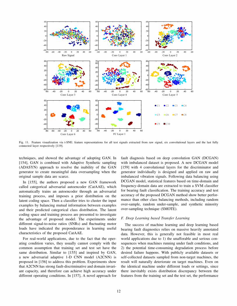
cluster together, which suggests that the following operations work as a correlation stage. This result matches with the ideaof the state-of-art domain adaptation method named CORAL, whose main idea is to decorrelate first and then re-correlate theresponses in networks to acquire better domain invariant features. However, our method doesn’t need to add any regulationterms to achieve this and doesn’t need any statistics information of target domain.

5. Conclusion

This paper proposes a new model named TICNN, to address the fault diagnosis problem. TICNN works directly on rawvibration signals without any time-consuming hand-crafted feature extraction process. TICNN has two main interferences,first-layer kernel dropout with constantly changing rate and very small batch training. With the help of data augmentation,the proposed TICNN model works well under noisy environment and performs well when the working load changes.

Results in Section 4 shows that, although state of the art DNN model could achieve pretty high accuracy on normal data-set, its performance suffer from rapid degradation under noisy environment or when working load changes. However,TICNN, with high classification accuracy, is also very robust to change of working load and noise.

Ensemble Learning has improved the stability and accuracy of the algorithm. In addition, Networks Visualizations areused to investigate the inner mechanism of the proposed TICNN model.

Compared with common denoising preprocessing algorithm and domain adaptation algorithm that requires additionalinformation, our algorithm does not need any subsidiary algorithm. Therefore, in future work, we can try combining somedenoising preprocessing and using information about the target domain to improve the performance of the proposed model.

Acknowledgements

This work was supported by National High-tech R&D Program of China (863 Program, No. 2015AA042201), National Nat-ural Science Foundation of China (No. 51275119), and Self-Planned Task (No. SKLRS201708A) of State Key Laboratory ofRobotics and System (HIT)”.

-80 -60 -40 -20 0 20 40 60-60

-40

-20

0

20

40

60

Raw Signal-60 -40 -20 0 20 40 60

-60

-40

-20

0

20

40

60

Conv Layer 1-60 -40 -20 0 20 40 60

-60

-40

-20

0

20

40

60

Conv Layer 2

-60 -40 -20 0 20 40 60-60

-40

-20

0

20

40

60

Conv Layer 3-60 -40 -20 0 20 40 60

-60

-40

-20

0

20

40

6070

Conv Layer 4-60 -40 -20 0 20 40 60

-60

-40

-20

0

20

40

60

Conv Layer 5

-80 -60 -40 -20 0 20 40 60-60

-40

-20

0

20

40

60

Conv Layer 6-60 -40 -20 0 20 40 60

-60

-40

-20

0

20

40

60

FC Layer 1

C1 C2 C3 C4

C5 C6 C7 C8

C9 C10

Fig. 11. Feature visualization via t-SNE: feature representations for all test signals extracted from raw signal, six convolutional layers and the last fully-connected layer respectively.

452 W. Zhang et al. /Mechanical Systems and Signal Processing 100 (2018) 439–453

Fig. 11. Feature visualization via t-SNE: feature representations for all test signals extracted from raw signal, six convolutional layers and the last fullyconnected layer respectively [119].

techniques, and showed the advantage of adopting GAN. In[154], GAN is combined with Adaptive Synthetic sampling(ADASYN) approach to resolve the inability of the GANgenerator to create meaningful data oversampling when theoriginal sample data are scarce.

In [155], the authors proposed a new GAN frameworkcalled categorical adversarial autoencoder (CatAAE), whichautomatically trains an autoencoder through an adversarialtraining process, and imposes a prior distribution on thelatent coding space. Then a classifier tries to cluster the inputexamples by balancing mutual information between examplesand their predicted categorical class distribution. The latentcoding space and training process are presented to investigatethe advantage of proposed model. The experiments underdifferent signal-to-noise ratios (SNRs) and fluctuating motorloads have indicated the preponderance in learning usefulcharacteristics of the proposed CatAAE.

For real-world applications, due to the fact that the oper-ating condition varies, they usually cannot comply with thecommon assumption that training set and test set have thesame distribution. Similar to [155] and inspired by GAN,a new adversarial adaptive 1-D CNN model (A2CNN) isproposed in [156] to address this problem. Experiments showthat A2CNN has strong fault-discriminative and domain invari-ant capacity, and therefore can achieve high accuracy underdifferent operating conditions. In [157], A novel approach for

fault diagnosis based on deep convolution GAN (DCGAN)with imbalanced dataset is proposed. A new DCGAN model[159] with 4 convolutional layers for the discriminator andgenerator individually is designed and applied on raw andimbalanced vibration signals. Following data balancing usingDCGAN model, statistical features based on time-domain andfrequency-domain data are extracted to train a SVM classifierfor bearing fault classification. The training accuracy and testaccuracy of the proposed DCGAN method show better perfor-mance than other class balancing methods, including randomover-sample, random under-sample, and synthetic minorityover-sampling technique (SMOTE).

F. Deep Learning based Transfer Learning

The success of machine learning and deep learning basedbearing fault diagnostics relies on massive heavily annotateddata. However, this is generally not feasible in most realworld applications due to 1) the unafforable and serious con-sequences when machines running under fault conditions, and2) the potential time-consuming degradation process beforedesired failure happens. With publicly available datasets orself-collected datasets sampled from non-target machines, theresult will naturally deteriorate on target machines. Even onthe identical machine under different loads or settings, sincethere inevitably exists distribution discrepancy between thefeatures from the training set and the test set, the performance

12

still suffers. Designed to tackle this practical and widely exis-tent issue in numerous areas, transfer learning has aroused ex-tensive attention in machine learning community, and varioustransfer learning frameworks are proposed based on classicalmachine learning algorithms [75]. A popular method amongall types of transfer learning approaches is domain adaptation.By exploring domain-invariant features, domain adaptationestablishes knowledge transfer from source domain to targetdomain [173]. Therefore, with labeled data from source do-main and unlabeled data from target domain, the distributiondiscrepancy between the two domains can be mitigated bydomain adaptation algorithms. In recent years, an integrationof deep learning and transfer learning approaches has beenwitnessed. Specially designed domain adaptation modules arecombined with deep learning architectures to endow domaintransfer ability while maintaining the extraordinary automaticfeature learning ability [173]–[177].

[176] proposed a novel framework WDCNN (Deep CNNwith wide first-layer kernels) combined with Adaptive BatchNormalization (AdaBN). It takes raw vibration signal as input.It’s based on a CNN architecture with wide kernels (64) in thefirst convolutional layer for better suppressing high frequencynoise. Then domain adaptation is implemented by extractingthe mean and variance of target domain signals and passing toAdaBN. It used CWRU dataset and conducted cross-domainexperiments when training in one working condition andtesting in another one. WDCNN has achieved the averageaccuracy of 90.0% outperforming FFT-DNN method 78.1%and reveived further improvement to 95.9% with AdaBN.When tested under noise environment (with additive whiteGaussian noise), WDCNN with AdaBN achieves 92.65% ac-curacy under -4(dB) SNR, in comparison with 66.95% withoutAdaBN.

In [174], a domain adaptation module facilitates a one-dimensional CNN to learn domain-invariant features by max-imizing domain recognition errors and minimizing probabilitydistribution distance. To validate the efficacy of the domainadaptation ability, 3 dataset including CWRU dataset, IMSdataset and railway locomotive (RL) bearing dataset are em-ployed. By training on one of the three datasets and testingon another one, the achieved average accuracy 86.3% hassurpassed the traditional CNN 53.1% and two another existingdomain adaptation frameworks 75.6% [171] and 78.8% [172].

[177] proposed a novel framework combining domainadaptation with deep generative network. It employs a 2stage structure. In the first stage, A 8-layer CNN componentincluding 3 convolutional layers with basic classifier is trainedas feature extractor while optimizing the classification errorunder source supervision; Then Nc − 1 (Nc is the number ofclasses) CNN components, each of which composes 3 convo-lutional layers and 3 dropout layers, are trained to minimizethe Maximum Mean Discrepancy. In the second stage, withthe feature extractor trained in the first stage, a cross-domainclassifier is trained and outputs the final diagnosis results.

G. Others

There are also numerous other DL methods employed forbearing fault diagnostics, some are based on new algorithms,some are mixture of the DL methods listed above. Forexample, in [160], a new large memory storage retrieval(LAMSTAR) neural network is proposed with one input layer,40 input SOM modules as hidden layers, and one decisionSOM module as output layer. More accurate classificationresults compared to conventional CNN are reported on var-ious operating conditions, especially at low speeds. In [161],both DBN and SAE are applied simultaneously to identifythe presence of a bearing fault. Other examples include amixture of CNN and DBN [162], deep residual network (DRN)[163], [164], deep stack network (DSN) [165], deep generativenetwork [78], RNN based autoencoder [166], sparse filtering[170], a new deep learning architecture capsule network [168]proposed by Hinton [167].

V. DISCUSSIONS ON DIFFERENT MACHINE LEARNINGALGORITHMS FOR BEARING FAULT DIAGNOSIS

A. Feature Extraction and Selection

To detect if a bearing fault is present, for a traditional MLalgorithm, the characteristic fault frequencies are calculatedbased on the rotor mechanical speed and the specific bearinggeometry, which serve as the fault features. This featurecalculation process is known as “feature engineering”. Theamplitude at these frequencies can then be monitored to trainvarious ML algorithms and identify any anomalies. However,such a technique may encounter many challenges that canaffect the classification accuracy.

1) Sliding: The frequency calculations have the assumptionthat there is no sliding, i.e., the rolling elements only rollon the raceways. Nevertheless, this is seldom the case.Often, a bearing undergoes a combination of rolling andsliding. As a consequence, the calculated frequencies maydiffer slightly, i.e. 1-2 percent, compared to the actualfrequencies.

2) Frequency interplay: If multiple types of bearing faultsoccur simultaneously, these faults will interact and thecharacteristic frequencies generated can add and subtractdue to superposition effects, obfuscating important fre-quencies.

3) External vibration: There is also the possibility of inter-ference induced due to additional sources of vibration,i.e. bearing looseness, which obscures useful features.

4) Observability: Some faults, such as lubrication relatedfaults, do not even manifest themselves as a characteristiccyclic frequency, which makes them very hard to detectvia traditional vibration spectral analysis techniques.

5) Sensitivity: The sensitivity of various features that arecharacteristic of a bearing defect may vary considerablyunder different operating conditions. A very thoroughand systematic “learning stage” is required to test thesensitivity of these frequencies on any desirable operatingcondition before it can be actually put into use.

13

TABLE IA SUMMARY OF DIFFERENT DEEP LEARNING ARCHITECTURE.

Architecture Description Characteristics

© MERL

MITSUBISHI ELECTRIC RESEARCH LABORATORIES

12/26/2018 CONFIDENTIAL 3

CNN

Convolutional Neural Network

• Well-suited for 2D data, i.e., images.

• Inspired by the neural-biologicalmodel of the visual cortex [107].

• RELU after convolutional layershelps accelerate convergence speed.

Pros:• Few neuron connections required with

respect to a typical ANN.• Many variants have been proposed:

LeNet-5 [112], LiftingNet [119], andinception net [122], etc.

Cons:• May require many layers to find an

entire hierarchy.• May require a large dataset of labeled

2D data.

© MERL

MITSUBISHI ELECTRIC RESEARCH LABORATORIES

12/26/2018 CONFIDENTIAL 4

Autoencoder Deep Autoencoder

• Mainly designed for feature extrac-tion or dimension reduction.

• Has the same number of input andoutput nodes.

• Unsupervised learning method aimingto recreate the input vector.

Pros:• Does not require labeled data.• Many variations have been proposed

to make the representation morenoise-resilient and robust: stacked de-noising AE [127], ensemble deep AE[132], and stacked sparse AE [134].

Cons:• Requires a pre-training stage.• Training may suffer from the vanish-

ing of errors.

© MERL

MITSUBISHI ELECTRIC RESEARCH LABORATORIES

12/26/2018 CONFIDENTIAL 5

DBN Deep Belief Network

• Composed of RBMs where each sub-network’s hidden layer serves as thevisible layer for the next.

• Has undirected connections just at thetop two layers.

• Allows unsupervised and supervisedtraining of the network.

Pros:• Proposes a layer-by-layer greedy

learning strategy to initialize the net-work.

• Tractable inferences minimizes thelikelihood directly.

Cons:• Training may be computationally ex-

pensive due to the initialization pro-cess and sampling.

© MERL

MITSUBISHI ELECTRIC RESEARCH LABORATORIES

12/29/2018 CONFIDENTIAL 7

Recurrent Neural Network

• An ANN capable of analyzing datastreams.

• LSTM re-vibrated the application ofRNNs.

• Suitable for applications where theoutput depends on the previous com-putations.

Pros:• Memorizes sequential events.• Models time dependencies.• Has shown great success in many ap-

plications: speech recognition, naturallanguage processing, video analysis.

Cons:• Learning issues are frequent due to

gradient vanishing/exploding.

© MERL

MITSUBISHI ELECTRIC RESEARCH LABORATORIES

12/27/2018 CONFIDENTIAL 7

GAN

Generative Adversarial Network

• Mainly designed for generate pho-tographs that look superficially au-thentic to human observers.

• Implemented by a system of genera-tive and discriminative networks.

• Semi-Supervised learning methodaiming to recreate the input vector.

Pros:• Requires almost no modifications

transferring to new applications.• Requires no Monte Carlo approxima-

tions to train.• Does not introduce deterministic bias.

Cons:• GAN training is unstable as it requires

finding a Nash equilibrium of a game.• Hard to learn to generate discrete

data, like text.

14

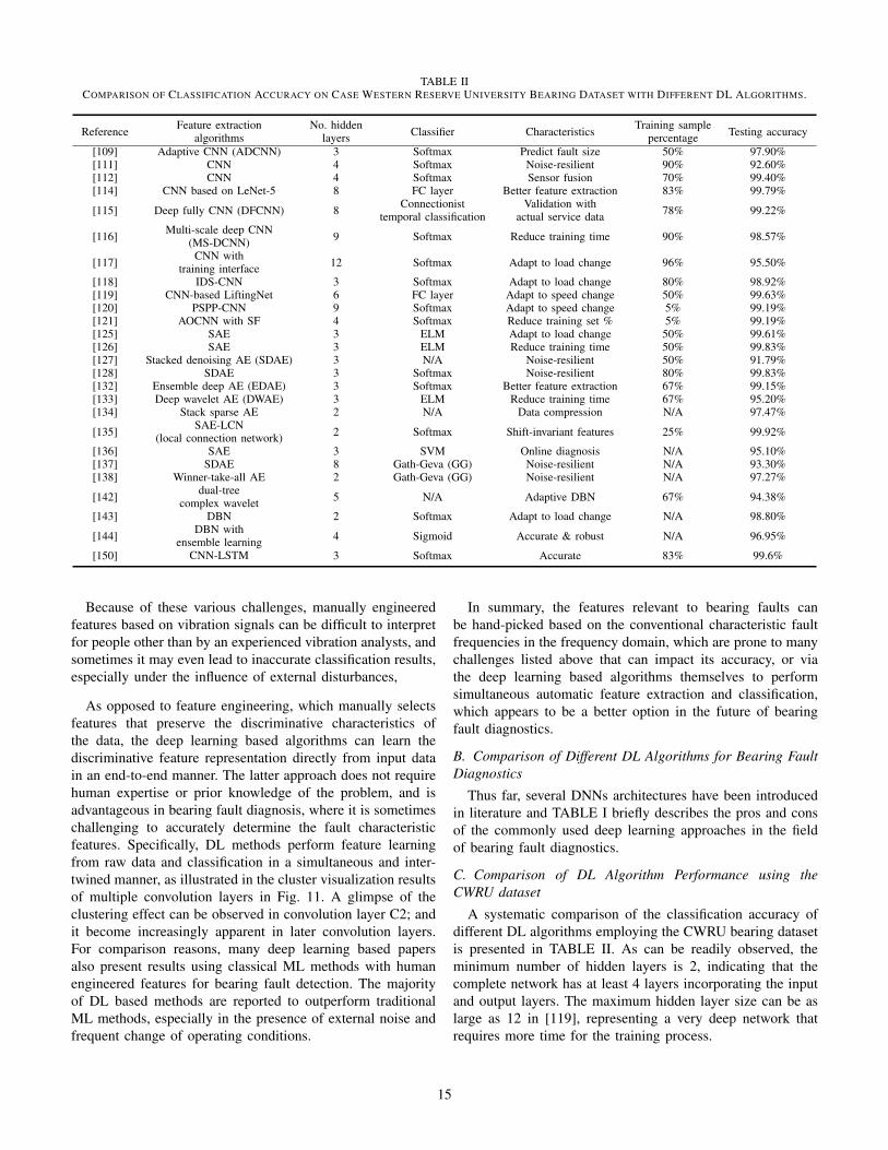
TABLE IICOMPARISON OF CLASSIFICATION ACCURACY ON CASE WESTERN RESERVE UNIVERSITY BEARING DATASET WITH DIFFERENT DL ALGORITHMS.

Reference Feature extractionalgorithms

No. hiddenlayers Classifier Characteristics Training sample

percentage Testing accuracy

[109] Adaptive CNN (ADCNN) 3 Softmax Predict fault size 50% 97.90%[111] CNN 4 Softmax Noise-resilient 90% 92.60%[112] CNN 4 Softmax Sensor fusion 70% 99.40%[114] CNN based on LeNet-5 8 FC layer Better feature extraction 83% 99.79%

[115] Deep fully CNN (DFCNN) 8 Connectionisttemporal classification

Validation withactual service data 78% 99.22%

[116] Multi-scale deep CNN(MS-DCNN) 9 Softmax Reduce training time 90% 98.57%

[117] CNN withtraining interface 12 Softmax Adapt to load change 96% 95.50%

[118] IDS-CNN 3 Softmax Adapt to load change 80% 98.92%[119] CNN-based LiftingNet 6 FC layer Adapt to speed change 50% 99.63%[120] PSPP-CNN 9 Softmax Adapt to speed change 5% 99.19%[121] AOCNN with SF 4 Softmax Reduce training set % 5% 99.19%[125] SAE 3 ELM Adapt to load change 50% 99.61%[126] SAE 3 ELM Reduce training time 50% 99.83%[127] Stacked denoising AE (SDAE) 3 N/A Noise-resilient 50% 91.79%[128] SDAE 3 Softmax Noise-resilient 80% 99.83%[132] Ensemble deep AE (EDAE) 3 Softmax Better feature extraction 67% 99.15%[133] Deep wavelet AE (DWAE) 3 ELM Reduce training time 67% 95.20%[134] Stack sparse AE 2 N/A Data compression N/A 97.47%

[135] SAE-LCN(local connection network) 2 Softmax Shift-invariant features 25% 99.92%

[136] SAE 3 SVM Online diagnosis N/A 95.10%[137] SDAE 8 Gath-Geva (GG) Noise-resilient N/A 93.30%[138] Winner-take-all AE 2 Gath-Geva (GG) Noise-resilient N/A 97.27%

[142] dual-treecomplex wavelet 5 N/A Adaptive DBN 67% 94.38%

[143] DBN 2 Softmax Adapt to load change N/A 98.80%

[144] DBN withensemble learning 4 Sigmoid Accurate & robust N/A 96.95%

[150] CNN-LSTM 3 Softmax Accurate 83% 99.6%

Because of these various challenges, manually engineeredfeatures based on vibration signals can be difficult to interpretfor people other than by an experienced vibration analysts, andsometimes it may even lead to inaccurate classification results,especially under the influence of external disturbances,

As opposed to feature engineering, which manually selectsfeatures that preserve the discriminative characteristics ofthe data, the deep learning based algorithms can learn thediscriminative feature representation directly from input datain an end-to-end manner. The latter approach does not requirehuman expertise or prior knowledge of the problem, and isadvantageous in bearing fault diagnosis, where it is sometimeschallenging to accurately determine the fault characteristicfeatures. Specifically, DL methods perform feature learningfrom raw data and classification in a simultaneous and inter-twined manner, as illustrated in the cluster visualization resultsof multiple convolution layers in Fig. 11. A glimpse of theclustering effect can be observed in convolution layer C2; andit become increasingly apparent in later convolution layers.For comparison reasons, many deep learning based papersalso present results using classical ML methods with humanengineered features for bearing fault detection. The majorityof DL based methods are reported to outperform traditionalML methods, especially in the presence of external noise andfrequent change of operating conditions.

In summary, the features relevant to bearing faults canbe hand-picked based on the conventional characteristic faultfrequencies in the frequency domain, which are prone to manychallenges listed above that can impact its accuracy, or viathe deep learning based algorithms themselves to performsimultaneous automatic feature extraction and classification,which appears to be a better option in the future of bearingfault diagnostics.

B. Comparison of Different DL Algorithms for Bearing FaultDiagnostics

Thus far, several DNNs architectures have been introducedin literature and TABLE I briefly describes the pros and consof the commonly used deep learning approaches in the fieldof bearing fault diagnostics.

C. Comparison of DL Algorithm Performance using theCWRU dataset

A systematic comparison of the classification accuracy ofdifferent DL algorithms employing the CWRU bearing datasetis presented in TABLE II. As can be readily observed, theminimum number of hidden layers is 2, indicating that thecomplete network has at least 4 layers incorporating the inputand output layers. The maximum hidden layer size can be aslarge as 12 in [119], representing a very deep network thatrequires more time for the training process.

15

The testing accuracies of all the DL algorithms are above95%, which validates the feasibility and effectiveness of ap-plying deep learning to bearing fault diagnostics. However, itis worthwhile to mention that the specific values of testingaccuracy are only demonstrated for an intuitive understandingfor the following reasons:

1) Generalization: Some of the DL methods with astonish-ing accuracies over 99% are generally applied on a veryspecific dataset at a fixed operating conedition, i.e., whenthe motor speed is 1797 rpm and load is 2 hp. However,this accuracy would suffer, and may drop to below 90%under the influence of noise and variation of motorspeed/load, which is common in practical applications.This is in spite of the relatively strong robustness tonoise disturbance of original DL algorithms (CNN, SAE,DBN, etc.), and their capabilities to learn fault featuresthrough a general-purpose learning architecture. It is alsoreported in [111] that CNN has a better built-in denoisingmechanism compared to other common DL algorithmssuch as SAE. Due to this limitation, some papers appliedstacked denoising AE (SDAE) [127], [128], [137] thatcan effectively increase accuracy for bearing fault iden-tification with a small signal to noise ratio (SNR), i.e.,SNR = 5 or 10.

2) Evaluation metrics: Regarding the selection of trainingsamples from the CWRU dataset, many papers did notguarantee a balanced sampling, which means the ratio ofdata samples selected from the healthy condition and thefaulty condition is not close to 1:1. In case of a significantunbalance, accuracy should not be used as the only metricto evaluate an algorithm [156]. Compared with accuracy,other metrics, such as precision and recall, should beintroduced to provide more details for evaluating thereliability of a fault identification model.

3) Randomness: Even these DL methods are using thesame dataset to perform classifications, the percentageof training data and test data are different. Even if thisdata distribution is identical, the training and test datamight be randomly selected from the CWRU bearingdataset. Therefore this comparison is not performed onthe common ground, since the classification accuracy issubject to change even with the same algorithm due torandomness in the training and test dataset selection.

4) Accuracy saturation: Most existing DL algorithms canachieve an excellent classification accuracy of over 95%while using the CWRU dataset, which seems to indicatethat this dataset contains relatively clear features that canbe readily extracted by a variety of DL methods. The su-periority of certain DL methods, however, is not apparent.Thus various perturbations on the original dataset needsto be performed, i.e., pollute the signals with randomnoise to test the algorithm’s denosing capability. In addi-tion, the level of background noise and all bearing defectsare artificially induced, which makes the validation resultsof different DL algorithms less convincing.

VI. RECOMMENDATIONS, SUGGESTIONS, AND FUTUREWORK DIRECTIONS

A. Recommendations and Suggestions

The successful implementation of machine learning anddeep learning algorithms on bearing fault diagnostics can beattributed to the strong correlations among features that followthe law of physics. For engineers and researchers consideringapplying ML/DL methods to solve their bearing problems athand, the authors suggest the following sequences to make thebest decision.

1) Examine the setup environment: Thoroughly examine theworking environment and all possible operating condi-tions of the setup. For example, indoor or outdoor, al-ways maintaining a fixed operating point or experiencingfrequent change of speed and load. For the simplestcase with an indoor and a single operating point setup,the traditional ML methods or even the frequency-basedanalytical models should suffice. For applications that aremore prone to external disturbances or constant changeof operating points, such as the motors fed by VFD con-verters in electric vehicles, more advanced deep learningapproaches should be considered, and certain denoisingblocks and extra layers should be considered to increasethe deep neural net robustness. Specifically, when theworkbench is exposed to a noisy environment, whichinduces a relatively inferior signal-to-noise ratio, specialdenoising components should be designed to increase therobustness of the architecture to external disturbances.

2) Sensors: Determine the number and type of sensors tobe mounted close to the bearings. For the traditionalfrequency based and ML based methods, one or twovibrations sensors mounted close to the bearing should besufficient. For deep learning based approaches, due to thefact that many algorithms such as CNN are mainly devel-oped for computer vision to handle the 2-D image data,multiple 1-D time-series data obtained by the sensors inthe bearing setup need to be stacked to form this 2-Ddata, or some prepossessing functions such as waveletpacket decomposition (WPD) need to be applied beforethe data is passed on to the deep neural nets. Therefore, itwould be better to have more than two vibration sensorsinstalled at the same time. In addition, other types ofsensors such as AE and stator current can be installedto form a multi-physics dataset to further improve theclassifier performance, especially during frequent andabrupt changes of the operating conditions.

3) Data Size: If the size of the collected dataset is notsufficient to train a deep learning model with goodgeneralization, the algorithms and their training processesshould be selected that make the most of the data andcomputing resources available. For example, the datasetaugmentation techniques such as GAN, and data randomsampling with replacement such as Boostrapping canbe implemented. Before actually collecting data fromthe bearing system setup, it is also useful to consider

16

beforehand how precise the classification results need tobe, in order to allow a useful interpretation of the neededsample size. [183] With the problem of small labeleddataset, another promising routine is to leverage unla-beled dataset, if possible, and apply the so-called semi-supervised learning paradigm by combining supervisedand unsupervised learning approaches.

B. Future Work Directions

As a future research trend, the authors suggest the followingdirections that are crucial to the advancement of the topicand the smooth transition from the research labs to real-worldapplications:

1) More complicated datasets: Apply more complicatedbearing datasets such as the Paderborn University dataset,since the accuracy saturation problem of the commonlyused CWRU dataset prevails.

2) From artificial to the real-world: Make attempts to predictthose natural faults with the algorithms trained by artifi-cial faults, which is actually a reasonable expectation forthe DL-based fault indicators to be applied in real-worldapplications.

VII. CONCLUSIONS

In this paper, a systematic review is conducted on existingliterature employing machine learning algorithms to motorbearing fault diagnostics. Special emphasis is placed on thedeep learning based approaches that has spurred the interestsof academia for the past five years. It is demonstrated that,despite the fact that the deep learning algorithms require alarge dataset to train, they can automatically perform adaptivefeature extractions on the bearing data without any prior exper-tise on fault characteristic frequencies or operating conditions,making them suitable for real-time bearing fault diagnostics.

REFERENCES

[1] M. E. H. Benbouzid, M. Vieira and C. Theys, “Induction motors’faults detection and localization using stator current advanced signalprocessing techniques,” IEEE Trans. Power Electron., vol. 14, no. 1,pp. 14–22, Jan. 1999.

[2] M. El Hachemi Benbouzid, “A review of induction motors signatureanalysis as a medium for faults detection,” IEEE Trans. Ind. Electron.,vol. 47, no. 5, pp. 984–993, Oct. 2000.

[3] P. Zhang, Y. Du, T. G. Habetler and B. Lu,“A survey of conditionmonitoring and protection methods for medium-voltage inductionmotors,” IEEE Trans. Ind. Appl., vol. 47, no. 1, pp. 34–46, Jan./Feb.2011.

[4] “Report of large motor reliability survey of industrial and commercialinstallations, Part I,” IEEE Trans. Ind. Appl., vol. IA–21, no. 4, pp.853-864, Jul./Aug. 1985.

[5] “Report of large motor reliability survey of industrial and commercialinstallations, Part II,” IEEE Trans. Ind. Appl., vol. IA–22, no. 4, pp.865–872, Jul./Aug. 1985.

[6] “Report of large motor reliability survey of industrial and commercialinstallations: Part 3,” IEEE Trans. Ind. Appl., vol. IA–23, no. 1, pp.153158, Jan./Feb. 1987.

[7] JEMA, “On recommended interval of updating induction motors”,2000 (in Japanese).

[8] T. Harris, Rolling Bearing Analysis, 3rd ed. Hoboken, NJ, USA:Wiley, 1991.

[9] J. Schmidhuber, “Deep learning in neural networks: An overview,”Neural Netw., vol. 61, pp. 85–117, Jan. 2015.

[10] J. Harmouche, C. Delpha and D. Diallo, “Improved fault diagnosis ofball bearings based on the global spectrum of vibration signals,” IEEETrans. Energy Convers., vol. 30, no. 1, pp. 376-383, March 2015.

[11] F. Immovilli, A. Bellini, R. Rubini and C. Tassoni, “Diagnosis ofbearing faults in induction machines by vibration or current signals:A critical comparison,” IEEE Trans. Ind. Appl., vol. 46, no. 4, pp.1350–1359, Jul./Aug. 2010.

[12] M. Kang, J. Kim and J. Kim, “An FPGA-based multicore system forreal-time bearing fault diagnosis using ultrasampling rate AE signals,”IEEE Trans. Ind. Electron., vol. 62, no. 4, pp. 2319–2329, Apr. 2015.

[13] A. Ming, W. Zhang, Z. Qin and F. Chu, “Dual-impulse response modelfor the acoustic emission produced by a spall and the size evaluationin rolling element bearings,” IEEE Trans. Ind. Electron, vol. 62, no.10, pp. 6606–6615, Oct. 2015.

[14] R. R. Schoen, T. G. Habetler, F. Kamran and R. G. Bartfield, “Motorbearing damage detection using stator current monitoring,” IEEETrans. Ind. Appl., vol. 31, no. 6, pp. 1274–1279, Nov./Dec. 1995.

[15] M. Blodt, P. Granjon, B. Raison and G. Rostaing,“Models for bearingdamage detection in induction motors using stator current monitor-ing,” IEEE Trans. Ind. Electron., vol. 55, no. 4, pp. 1813–1822, Apr.2008.

[16] D. Lopez-Perez and J. Antonino-Daviu, “Application of infraredthermography to failure detection in industrial induction motors: casestories,” IEEE Trans. Ind. Appl., vol. 53, no. 3, pp. 1901–1908,May/June 2017.

[17] E. T. Esfahani, S. Wang and V. Sundararajan, “Multisensor wirelesssystem for eccentricity and bearing fault detection in inductionmotors,” IEEE/ASME Trans. Mechatronics, vol. 19, no. 3, pp. 818-826, June 2014.

[18] B. Yazici and G. B. Kliman, “Adaptive, on line, statistical method andapparatus for motor bearing fault detection by passive motor currentmonitoring,” U.S. Patent 5 726 905, Sep. 27, 1995.

[19] W. Xin, “A hybrid intelligent technique for induction motor condi-tion monitoring,” Ph.D. dissertation, Dept. Mech. Des. Eng., Univ.Portsmouth, Portsmouth, U.K., 2011.

[20] S. Singh, C. Q. Howard, and C. Hansen, “An extensive review ofvibration modelling of rolling element bearings with localised andextended defects,” J. Sound Vib., vol. 357, pp. 300–330, 2015

[21] H. Cao, L. Niu, S. Xia, and X. Chen, “Mechanical model develop-ment of rolling bearing-rotor systems: A review,” Mech. Syst. SignalProcess., vol. 102, pp. 37–58, Mar. 2018.

[22] P. D. McFadden and J. D. Smith, “Model for the vibration producedby a single point defect in rolling element bearing,” J. Sound Vib.,vol. 96, no. 1, pp. 69–82, 1984.

[23] N. Tandon and A. Choudhury, “An analytical model for the predictionof the vibration response of rolling element bearings due to a localizeddefect,” J. Sound Vib., vol. 205, no. 3, pp. 275–292, Aug. 1997.

[24] Z. Kıral and H. Karagulle, “Vibration analysis of rolling elementbearings with various defects under the action of an unbalanced force,”Mech. Syst. Signal Process., vol. 20, pp. 1967–1991, 2006.

[25] S. Singh et al, “Analyses of contact forces and vibration response fora defective rolling element bearing using an explicit dynamics finiteelement model,” J. Sound Vib., vol. 333, pp. 5356–5377, 2014.

[26] (2018, December). Case Western Reserve University(CWRU) Bearing Data Center, [Online]. Available:https://csegroups.case.edu/bearingdatacenter/pages/welcome-case-western-reserve-university-bearing-data-center-website.

[27] (2018, December). NVIDIA TESLA: The Worlds Most Ad-vanced Data Center GPUs., [Online]. Available: https://mb.uni-paderborn.de/kat/forschung/datacenter/bearing-datacenter/.

[28] (2018, December). IEEE PHM 2012 Data Challenge bearing dataset,[Online]. Available: http://data-acoustics.com/measurements/bearing-faults/bearing-6/.

[29] P. Nectoux et al., Pronostia: An experimental platform for bearingsaccelerated life test, in Proc. IEEE Int. Conf. Prognostics HealthManag., Denver, CO, USA, 2012, pp. 18.

[30] M. A. Awadallah and M. M. Morcos, “Application of AI tools infault diagnosis of electrical machines and drives – an overview,” IEEETrans. Energy Convers., vol. 18, no. 2, pp. 245–251, June 2003.

[31] F. Filippetti, G. Franceschini, C. Tassoni and P. Vas, “Recent develop-ments of induction motor drives fault diagnosis using AI techniques,”IEEE Trans. Ind. Electron., vol. 47, no. 5, pp. 994–1004, Oct. 2000.

[32] L. Batista, B. Badri, R. Sabourin, and M. Thomas, “A classifier fusionsystem for bearing fault diagnosis,” Expert Syst. Appl., vol. 40, no. 7,pp. 6788–6797, Dec. 2013.

17

[33] R. Liu, B. Yang, E. Zio, and X. Chen, “Artificial intelligence forfault diagnosis of rotating machinery: A review,” Mech. Syst. SignalProcess., vol. 108, pp. 33–47, Aug. 2018.

[34] S. Khan and T. Yairi, “A review on the application of deep learningin system health management,” Mech. Syst. Signal Process., vol. 107,pp. 241–265, 2018.

[35] M. Cerrada et al., “A review on data-driven fault severity assessmentin rolling bearings,” Mech. Syst. Signal Process., vol. 99, pp. 169–196,Jan. 2018.

[36] R. Zhao, R. Yan, Z. Chen, K. Mao, P. Wang, and R.-X. Gao, “Deeplearning and its applications to machine health monitoring,” Mech.Syst. Signal Process., vol. 115, pp. 213–237, 2019.

[37] M.-Y. Chow, P. M. Mangum and S. O. Yee, “A neural networkapproach to real-time condition monitoring of induction motors,”IEEE Trans. Ind. Electron., vol. 38, no. 6, pp. 448–453, Dec. 1991.

[38] R. R. Schoen, B. K. Lin, T. G. Habetler, J. H. Schlag and S. Farag,“An unsupervised, on-line system for induction motor fault detectionusing stator current monitoring,” IEEE Trans. Ind. Appl., vol. 31, no.6, pp. 1280–1286, Nov.-Dec. 1995.

[39] B. Li, M.-Y. Chow, Y. Tipsuwan and J. C. Hung, “Neural-network-based motor rolling bearing fault diagnosis,” IEEE Trans. Ind. Elec-tron., vol. 47, no. 5, pp. 1060–1069, Oct. 2000.

[40] M. Cococcioni, B. Lazzerini and S. L. Volpi, “Robust diagnosis ofrolling element bearings based on classification techniques,” IEEETrans. Ind. Informat., vol. 9, no. 4, pp. 2256–2263, Nov. 2013.

[41] S. Qian, X. Yang, J. Huang and H. Zhang, “Application of newtraining method combined with feedforward artificial neural networkfor rolling bearing fault diagnosis,” in Proc. Int. Conf. MechatronicsMach. Vision in Practice (M2VIP), Nanjing, China, 2016, pp. 1–6.

[42] S. Lu and X. Wang, “PCA-based feature selection scheme for machinedefect classification,” IEEE Trans. Instrum. Mea., vol. 53, no. 6, pp.1517–1525, Dec. 2004.

[43] X. Zhang, R. Xu, C. Kwan, S.-Y. Liang, Q. Xie and L. Haynes, “Anintegrated approach to bearing fault diagnostics and prognostics,” inProc. American Control Conf., Portland, OR, USA, 2005, pp. 2750–2755 vol. 4.

[44] M. Xia, F. Kong and F. Hu, “An approach for bearing fault diagnosisbased on PCA and multiple classifier fusion,” in Proc. IEEE Joint Int.Inf. Technol. AI Conf., Chongqing, China, 2011, pp. 321–325.

[45] J. Harmouche, C. Delpha and D. Diallo, “A global approach for theclassification of bearing faults conditions using spectral features,” inProc. 39th Annu. Conf. IEEE Ind. Electron. Soc. (IECON’13), Vienna,Austria, 2013, pp. 7352–7357.

[46] X. Xue and J. Zhou, “A hybrid fault diagnosis approach based onmixed-domain state features for rotating machinery,” ISA Trans., vol.66, pp. 284–295, 2017.

[47] D. He, R. Li, J. Zhu and M. Zade, “Data mining based full ceramicbearing fault diagnostic system using AE sensors,” IEEE Trans.Neural Netw., vol. 22, no. 12, pp. 2022–2031, Dec. 2011.

[48] M. M. Ettefagh, M. Ghaemi and M. Yazdanian Asr, “Bearing faultdiagnosis using hybrid genetic algorithm K-means clustering,” inProc. Int. Symp. Innov. Intell. Syst. Appli. (INISTA), Alberobello, Italy,2014, pp. 84–89.

[49] J. Tian, C. Morillo, M. H. Azarian and M. Pecht, “Motor bearingfault detection using spectral Kurtosis-based feature extraction cou-pled with K-nearest neighbor distance analysis,” IEEE Trans. Ind.Electron., vol. 63, no. 3, pp. 1793–1803, Mar. 2016.

[50] T. W. Rauber, F. de Assis Boldt and F. M. Varejao, “Heterogeneousfeature models and feature selection applied to bearing fault diagno-sis,” IEEE Trans. Ind. Electron., vol. 62, no. 1, pp. 637–646, Jan.2015.

[51] A. Rojas and A. K. Nandi, “Detection and classification of rolling-element bearing faults using support vector machines,” in Proc. IEEEWorkshop on Mach. Learning Signal Process., Mystic, CT, USA,2005, pp. 153–158.

[52] K. Teotrakool, M. J. Devaney and L. Eren, “Bearing fault detectionin adjustable speed drives via a support vector machine with featureselection using a genetic algorithm,” in Proc. IEEE Instrum. Mea.Technol. Conf., Victoria, BC, Canada, 2008, pp. 1129–1133.

[53] P.Konar, and P. Chattopadhyay, “Bearing fault detection of inductionmotor using wavelet and Support Vector Machines (SVMs),” Appl.Soft Comput., vol. 11, no. 6, pp. 4203–4211, Sep. 2011.

[54] T. Benkedjouh, K. Medjaher, N. Zerhouni and S. Rechak, “Faultprognostic of bearings by using support vector data description,” inProc. IEEE Conf. Progno. Health Manag., Denver, CO, USA, 2012,pp. 1–7.

[55] M. Kang, J. Kim, J. Kim, A. C. C. Tan, E. Y. Kim and B. Choi,“Reliable fault diagnosis for low-speed bearings using individuallytrained support vector machines with kernel discriminative featureanalysis,” IEEE Trans. Power Electron., vol. 30, no. 5, pp. 2786–2797, May 2015.

[56] S. E. Pandarakone, Y. Mizuno and H. Nakamura, “Distinct faultanalysis of induction motor bearing using frequency spectrum deter-mination and support vector machine,” IEEE Trans. Ind. Appl., vol.53, no. 3, pp. 3049–3056, May-June 2017.

[57] F. B. Abid, S. Zgarni and A. Braham, “Bearing fault detection ofinduction motor using SWPT and DAG support vector machines,”in Proc. 42nd Annu. Conf. IEEE Ind. Electron. Soc. (IECON’16),Florence, Italy, 2016, pp. 1476–1481.

[58] H. Hassani, J. Zarei, M. M. Arefi and R. Razavi-Far, “zSlices-based general type-2 fuzzy fusion of support vector machines withapplication to bearing fault detection,” IEEE Trans. Ind. Electron.,vol. 64, no. 9, pp. 7210–7217, Sept. 2017.

[59] S. Kang, L. Cui, Y. Wang, F. Li and V. I. Mikulovich, “Method ofassessing the multi-state of a rolling bearing based on CFOA-HSVMtwo measures combination,” in Proc. Prog. Syst. Health Manag. Conf.(PHM), Beijing, China, 2017, pp. 1–5.

[60] B. R. Nayana and P. Geethanjali, “Analysis of statistical time-domainfeatures effectiveness in identification of bearing faults from vibrationsignal,” IEEE Sensors J., vol. 17, no. 17, pp. 5618–5625, 1 Sept.1,2017.

[61] M. Elforjani and S. Shanbr, “Prognosis of bearing acoustic emissionsignals using supervised machine learning,” IEEE Trans. Ind. Elec-tron., vol. 65, no. 7, pp. 5864–5871, July 2018.

[62] W. Song and J. Xiang, “A method using numerical simulation andsupport vector machine to detect faults in bearings,” in Proc. 2017Int. Conf. Sens. Diagn., Prog. Control (SDPC), Shanghai, China, 2017,pp. 603–607.

[63] S. E. Pandarakone, Y. Mizuno and H. Nakamura, “Evaluating theprogression and orientation of scratches on outer-raceway bearingusing a pattern recognition method,” IEEE Trans. Ind. Electron., vol.66, no. 2, pp. 1307–1314, Feb. 2019.

[64] F. Ben Abid, S. Zgarni and A. Braham, “Distinct bearing faultsdetection in induction motor by a hybrid optimized SWPT and aiNet-DAG SVM,” IEEE Trans. Energy Convers., vol. PP, no. PP, pp. PP–PP,2018.

[65] C. Chen, B. Zhang and G. Vachtsevanos, “Prediction of machinehealth condition using neuro-fuzzy and Bayesian algorithms,” IEEETrans. Instrum. Mea., vol. 61, no. 2, pp. 297–306, Feb. 2012.

[66] A. Soualhi and S. Taleb, “Data fusion for fault severity estimation ofball bearings,” in Proc. IEEE Int. Conf. Ind. Technol. (ICIT), Lyon,France, 2018, pp. 2105–2110.

[67] A. S. Raj and N. Murali, “Early classification of bearing faultsusing morphological operators and fuzzy inference,” IEEE Trans. Ind.Electron., vol. 60, no. 2, pp. 567–574, Feb. 2013.

[68] J. Wu, C. Wu, S. Cao, S. W. Or, C. Deng and X. Shao, “Degradationdata-driven time-to-failure prognostics approach for rolling elementbearings in electrical machines,” IEEE Trans. Ind. Electron., vol. 66,no. 1, pp. 529–539, Jan. 2019.

[69] X. Zhang, J. Kang and T. Jin, “Degradation modeling and maintenancedecisions based on Bayesian belief networks,” IEEE Trans. Rel., vol.63, no. 2, pp. 620–633, June 2014.

[70] J. Qu, Z. Zhang, and T. Gong, “A novel intelligent method formechanical fault diagnosis based on dual-tree complex wavelet packettransform and multiple classifier fusion,” NeuroComput., vol. 171, pp.831–853, 2017.

[71] W. Li, S. Zhang and G. He, “Semisupervised distance-preserving self-organizing map for machine-defect detection and classification,” IEEETrans. Instrum. Mea., vol. 62, no. 5, pp. 869–879, May 2013.

[72] Z. Zhou, J. Chen, Y. Zi and X. Chen, “Multi-domain descriptionmethod for bearing fault recognition in varying speed condition,”in Proc. 42nd Annu. Conf. IEEE Ind. Electron. Soc. (IECON’16),Florence, Italy, 2016, pp. 423–428.

[73] Q. Tong et al., “A fault diagnosis approach for rolling elementbearings based on RSGWPT-LCD bi-layer screening and extremelearning machine,” in IEEE Access, vol. 5, pp. 5515–5530, 2017.

18

[74] Q. Hu, A. Qin, Q. Zhang, J. He and G. Sun, “Fault diagnosisbased on weighted extreme learning machine with wavelet packetdecomposition and KPCA,” IEEE Sensors J., vol. 18, no. 20, pp.8472–8483, 15 Oct. 15, 2018.

[75] S. Pan and Q. Yang. “A survey on transfer learning,” in IEEETransactions on Knowledge and Data Engineering, October 2009

[76] F. Shen, C. Chen, R. Yan and R. X. Gao, “Bearing fault diagnosisbased on SVD feature extraction and transfer learning classification,”in Proc. Prog. Syst. Health Manag. Conf. (PHM), Beijing, China,2015, pp. 1–6.

[77] R. Zhang, H. Tao, L. Wu and Y. Guan, “Transfer learning with neuralnetworks for bearing fault diagnosis in changing working conditions,”in IEEE Access, vol. 5, pp. 14347–14357, 2017.

[78] A New Transfer Learning Method and its Application on RotatingMachine Fault Diagnosis Under Variant Working Conditions

[79] M. Cococcioni, B. Lazzerini and S. L. Volpi, “Robust diagnosis ofrolling element bearings based on classification techniques,” IEEETrans. Ind. Informat., vol. 9, no. 4, pp. 2256–2263, Nov. 2013.

[80] X. Zhao and M. Jia, “Fault diagnosis of rolling bearing based onfeature reduction with global-local margin Fisher analysis,” Neuro-comput., vol. 315, pp. 447–464, 2018.

[81] X. Jin, M. Zhao, T. W. S. Chow and M. Pecht, “Motor bearing faultdiagnosis using trace ratio linear discriminant analysis,” IEEE Trans.Ind. Electron., vol. 61, no. 5, pp. 2441–2451, May 2014.

[82] Z. Wang, Q. Zhang, J. Xiong, M. Xiao, G. Sun and J. He, “Faultdiagnosis of a rolling bearing using wavelet packet denoising andrandom forests,” IEEE Sensors J., vol. 17, no. 17, pp. 5581–5588, 1Sept.1, 2017.

[83] T. Yang, H. Pen, Z. Wang and C. S. Chang, “Feature knowledgebased fault detection of induction motors through the analysis of statorcurrent data,” IEEE Trans. Instrum. Mea., vol. 65, no. 3, pp. 549-558,Mar. 2016.

[84] Y. Lei, F. Jia, J. Lin, S. Xing and S. X. Ding, “An intelligentfault diagnosis method using unsupervised feature learning towardsmechanical big data,” IEEE Trans. Ind. Electron., vol. 63, no. 5, pp.3137–3147, May 2016.

[85] M. D. Prieto, G. Cirrincione, A. G. Espinosa, J. A. Ortega andH. Henao, “Bearing fault detection by a novel condition-monitoringscheme based on statistical-time features and neural networks,” IEEETrans. Ind. Electron., vol. 60, no. 8, pp. 3398–3407, Aug. 2013.

[86] B. Yao, P. Zhen, L. Wu and Y. Guan, “Rolling element bearing faultdiagnosis using improved manifold learning,” in IEEE Access, vol. 5,pp. 6027–6035, 2017.

[87] B. Wang, H. Pan, and W. Yang, “A complementary approach for faultdiagnosis of rolling bearing using canonical variate analysis basedshort-time energy feature,” J. Vib. Control, vol. 24, no. 18, pp. 4195–4210, Sep. 2018.

[88] B. Zhang, C. Sconyers, C. Byington, R. Patrick, M. E. Orchard and G.Vachtsevanos, “A probabilistic fault detection approach: Applicationto bearing fault detection,” IEEE Trans. Ind. Electron., vol. 58, no. 5,pp. 2011–2018, May 2011.

[89] J. Yu, “Local and nonlocal preserving projection for bearing defectclassification and performance assessment,” IEEE Trans. Ind. Elec-tron., vol. 59, no. 5, pp. 2363–2376, May 2012.

[90] H. Xue, M. Wang, Z. Li and P. Chen, “Fault feature extraction basedon artificial hydrocarbon network for sealed deep groove ball bearingsof in-wheel motor,” in Proc. 2017 Progn. Syst. Health Manag. Conf.(PHM-Harbin), Harbin, China, 2017, pp. 1–5.

[91] R. Razavi-Far, M. Farajzadeh-Zanjani and M. Saif, “An integratedclass-imbalanced learning scheme for diagnosing bearing defects ininduction motors,” IEEE Trans. Ind. Informat., vol. 13, no. 6, pp.2758–2769, Dec. 2017.

[92] J. Tian, M. H. Azarian, M. Pecht, G. Niu and C. Li, “An ensemblelearning-based fault diagnosis method for rotating machinery,” inProc. 2017 Progn. Syst. Health Manag. Conf. (PHM-Harbin), Harbin,China, 2017, pp. 1–6.

[93] V. Vakharia, V. K. Gupta and P. K. Kankar, “Ball bearing fault diag-nosis using supervised and unsupervised machine learning methods,”Int. J. Acoust. Vib., vol. 20, no. 4, pp. 244–250, 2015.

[94] D. He, R. Li and J. Zhu, “Plastic bearing fault diagnosis based on atwo-step data mining approach,” IEEE Trans. Ind. Electron., vol. 60,no. 8, pp. 3429–3440, Aug. 2013.

[95] M. Van and H. Kang, “Bearing-fault diagnosis using non-local meansalgorithm and empirical mode decomposition-based feature extraction

and two-stage feature selection,” IET Sci., Mea. & Technol., vol. 9,no. 6, pp. 671–680, Sep. 2015.

[96] J. B. Ali, N. Fnaiech, L. Saidi, B. Chebel-Morello, and F. Fnaiech,“Application of empirical mode decomposition and artificial neuralnetwork for automatic bearing fault diagnosis based on vibrationsignals,” Appl. Acoust., vol. 89, pp. 16–27, Mar. 2015.

[97] X. Yu, F. Dong, E. Ding, S. Wu and C. Fan, “Rolling bearing faultdiagnosis using modified LFDA and EMD with sensitive featureselection,” in IEEE Access, vol. 6, pp. 3715–3730, 2018.

[98] Q. Fu, B. Jing, P. He, S. Si and Y. Wang, “Fault feature selectionand diagnosis of rolling bearings based on EEMD and optimizedElman AdaBoost algorithm,” IEEE Sensors J., vol. 18, no. 12, pp.5024–5034, 15 June 15, 2018.

[99] C. Chen, F. Shen, and R. Yan, “Topic correlation analysis for bearingfault diagnosis under variable operating conditions,” J. Phys.: Conf.Ser., vol. 842, art no. 012045, pp. 1–9, 2017.

[100] X. Zhao and M. Jia, “A novel intelligent method for bearing faultdiagnosis based on affinity propagation clustering and adaptive featureselection,” Knowl.-Based Syst., vol. 116, pp. 1–12, 2017.

[101] Y. Lu, R. Xie, and S.-Y. Liang, “Adaptive online dictionary learningfor bearing fault diagnosis,” Int. J. Adv. Manuf. Technol., pp. 1–8, Oct.2018.

[102] Sparse classification based on dictionary learning for planet bearingfault identification

[103] A. Ng, “CS229 course notes: Deep learning”, Stanford University,Fall 2018.

[104] (2018, December). NVIDIA TESLA: The Worlds MostAdvanced Data Center GPUs., [Online]. Available:http://wild.link/nvidia/ANrTCA.

[105] (2018, December). Amazon Mechanical Turk, [Online]. Available:https://www.mturk.com/.

[106] M. Raghu, B. Poole, J Kleinberg, S. Ganguli, and J. Sohl-Dickstein,“On the expressive power of deep neural networks,” arXiv preprintarXiv:1606.05336, 2016.

[107] K. Fukushima, “Neocognitron: A self-organizing neural networkmodel for a mechanism of pattern recognition unaffected by shiftin position,” Biolog. Cybernetics, vol. 36, pp. 193–202, 1980.

[108] S. Singh, C. Q. Howard, and C. Hansen, “Convolutional neuralnetwork based fault detection for rotating machinery,” J. Sound Vib.,vol. 377, pp. 331–345, 2016.

[109] X. Guo, L. Chen, and C. Shen, “Hierarchical adaptive deep convo-lution neural network and its application to bearing fault diagnosis,”Meas., vol. 93, pp. 490–502, 2016.

[110] R. Liu, G. Meng, B. Yang, C. Sun and X. Chen, “Dislocated timeseries convolutional neural architecture: An intelligent fault diagnosisapproach for electric machine,” IEEE Trans. Ind. Informat., vol. 13,no. 3, pp. 1310–1320, June 2017.

[111] C. Lu, Z. Wang, and Bo Zhou, “Intelligent fault diagnosis of rollingbearing using hierarchical convolutional network based health stateclassification,” Adv. Eng. Informat., vol. 32, pp. 139–157, 2017.

[112] M. Xia, T. Li, L. Xu, L. Liu and C. W. de Silva, “Fault diagnosis forrotating machinery using multiple sensors and convolutional neuralnetworks,” IEEE/ASME Trans. Mechatronics, vol. 23, no. 1, pp. 101–110, Feb. 2018.

[113] Y. LeCun, L. Bottou, Y. Bengio, and P. Haffner, Gradient basedlearning applied to document recognition, Proceedings of the IEEE,vol. 86, no. 11, pp. 2278–2324, Nov. 1998.

[114] L. Wen, X. Li, L. Gao and Y. Zhang, “A new convolutional neuralnetwork-based data-driven fault diagnosis method,” IEEE Trans. Ind.Electron., vol. 65, no. 7, pp. 5990–5998, July 2018.

[115] W. Zhang, F. Zhang, W. Chen, Y. Jiang and D. Song, “Fault staterecognition of rolling bearing based fully convolutional network,”Comput. in Sci. & Eng., vol. PP, no. PP, pp. PP–PP, 2018.

[116] Z. Zhuang and Q. Wei, “Intelligent fault diagnosis of rolling bearingusing one-dimensional multi-scale deep convolutional neural networkbased health state classification,” in Proc. 2018 IEEE 15th Int. Conf.Netw., Sens. & Control (ICNSC), Zhuhai, China, 2018, pp. 1–6.

[117] W. Zhang, C. Li, G. Peng, Y. Chen, Z. Zhang, “A deep convolutionalneural network with new training methods for bearing fault diagnosisunder noisy environment and different working load,” Mech. Syst.Signal Process., vol. 100, pp. 439–458, 2018.

[118] S. Li, G. Liu, X. Tang, J. Lu, and J. Hu, “An ensemble deepconvolutional neural network model with improved D-S evidencefusion for bearing fault diagnosis,” Sensors, vol. 17, art. no. 1729,Jul. 2017.

19

[119] J. Pan, Y. Zi, J. Chen, Z. Zhou and B. Wang, “LiftingNet: A noveldeep learning network with layerwise feature learning from noisymechanical data for fault classification,” IEEE Trans. Ind. Electron.,vol. 65, no. 6, pp. 4973–4982, June 2018.

[120] S. Guo, T. Yang, W. Gao, C. Zhang, and Y. Zhang, “An intelligentfault diagnosis method for bearings with variable rotating speed basedon Pythagorean spatial pyramid pooling CNN,” Sensors, vol. 18, art.no. 3857, Nov. 2018.

[121] W. Qian, S. Li, J. Wang, Z. An, ans X. Jiang, “An intelligent faultdiagnosis framework for raw vibration signals: adaptive overlappingconvolutional neural network,” Meas. Sci. Technol., vol. 29, no. 6, art.no 095009, Aug. 2018.

[122] Y. Chen, G. Peng, C. Xie, W. Zhang, C. Li, and S. Liu, “ACDIN:Bridging the gap between artificial and real bearing damages forbearing fault diagnosis,” Neurocomput., vol. 294, pp. 61–71, 2018.

[123] L. Guo, Y. Lei, N. Li and S. Xing, “Deep convolution feature learningfor health indicator construction of bearings,” in Proc. 2017 Progn.Syst. Health Manag. Conf. (PHM-Harbin), Harbin, China, 2017, pp.1–6.

[124] X. Ding and Q. He, “Energy-fluctuated multiscale feature learningwith deep ConvNet for intelligent spindle bearing fault diagnosis,”IEEE Trans. Instrum. Meas., vol. 66, no. 8, pp. 1926–1935, Aug.2017.

[125] F. Jia, Y. Lei, J. Lin, X. Zhou, and N. Lu, “Deep neural networks: Apromising tool for fault characteristic mining and intelligent diagnosisof rotating machinery with massive data,” Mech. Syst. Signal Process.,vol. 100, pp. 743–765, 2016.

[126] W. Mao, J. He, Y. Li, and Y. Yan, “Bearing fault diagnosis with auto-encoder extreme learning machine: A comparative study,” Proc. Inst.Mech. Eng. C, J. Mech. Eng. Sci., vol. 231, no. 8, pp. 1560–1578,2016.

[127] C. Lu, Z.-Y Wang, W.-L. Qin, J. Ma, “Fault diagnosis of rotarymachinery components using a stacked denoising autoencoder-basedhealth state identification,” Signal Process., vol. 130, pp. 377–388,2017.

[128] X. Guo, C. Shen, and L. Chen, “Deep fault recognizer: An integratedmodel to denoise and extract features for fault diagnosis in rotatingmachinery,” Appl. Sci., 2017, vol. 7. no. 41, pp. 1–17.

[129] H. Shao, H. Jiang, H. Zhao, and F. Wang, “A novel deep autoencoderfeature learning method for rotating machinery fault diagnosis,” Mech.Syst. Signal Process., vol. 95, pp. 187–204, 2017.

[130] H. Shao, H. Jiang, F. Wang, and H. Zhao, “An enhancement deepfeature fusion method for rotating machinery fault diagnosis,” Mech.Syst. Signal Process., vol. 102, pp. 278–297, 2017.

[131] F. Wang, B. Dun, G. Deng, H. Li and Q. Han, “A deep neuralnetwork based on kernel function and auto-encoder for bearing faultdiagnosis,” in Proc. IEEE Int. Instrum. Meas. Technol. Conf. (I2MTC),Houston, TX, USA, 2018, pp. 1–6.

[132] H. Shao, H. Jiang, Y. Lin, and X. Li, “A novel method for intelli-gent fault diagnosis of rolling bearings using ensemble deep auto-encoders,” Knowl.-Based Syst., vol. 119, pp. 200–220, 2018.

[133] H. Shao, H. Jiang, X. Li, S. Wu, “Intelligent fault diagnosis ofrolling bearing using deep wavelet auto-encoder with extreme learningmachine,” Knowl.-Based Syst., vol. 140, pp. 1–14, 2018.

[134] J. Sun, C. Yan and J. Wen, “Intelligent bearing fault diagnosis methodcombining compressed data acquisition and deep learning,” IEEETrans. Instrum. Meas., vol. 67, no. 1, pp. 185–195, Jan. 2018.

[135] F. Jia, Y. Lei, L. Guo, J. Lin, and S. Xing, “A neural network con-structed by deep learning technique and its application to intelligentfault diagnosis of machines,” Neurocomput., vol. 272, pp. 619–628,2018.

[136] W. Mao, S. Tian, X. Liang, and J. He, “Online bearing fault diagnosisusing support vector machine and stacked auto-encoder,” in Proc.IEEE Int. Conf. Prognost. Health Manag. (ICPHM), Seattle, WA,2018, pp. 1–7.

[137] F. Xu, W. P. Tse, and Y.-L. Tse, “Roller bearing fault diagnosisusing stacked denoising autoencoder in deep learning and Gath-Gevaclustering algorithm without principal component analysis and datalabel,” Appl. Soft Comput. J., vol. PP, pp. PP–PP, 2018.

[138] C. Li, W. Zhang, G. Peng, and S. Liu, “Bearing fault diagnosis usingfully-connected winner-take-all autoencoder,” IEEE Access, vol. 6, pp.6103–6115, 2018.

[139] Y. Bengio, Learning deep architectures for AI, Foundations andTrends in Machine Learning, vol. 2, no. 1, pp. 1–127, 2009.

[140] Z. Chen and W. Li, “Multisensor feature fusion for bearing faultdiagnosis using sparse autoencoder and deep belief network,” IEEETrans. Instrum. Meas., vol. 66, no. 7, pp. 1693–1702, July 2017.

[141] S. Dong, Z. Zhang, G. Wen, S. Dong, Z. Zhang and G. Wen, “Designand application of unsupervised convolutional neural networks inte-grated with deep belief networks for mechanical fault diagnosis,” inProc. 2017 Progn. Syst. Health Manag. Conf. (PHM-Harbin), Harbin,China, 2017, pp. 1–7.

[142] D. T. Hoang and H. J. Kang, “Rolling bearing fault diagnosis usingadaptive deep belief network with dual-tree complex wavelet packet,”ISA Trans., vol. 69, pp. 187–201, 2017.

[143] D.-T. Hoang and H.-J. Kang, “Deep belief network and dempster-shafer evidence theory for bearing fault diagnosis,” in Proc. IEEE27th Int. Sym. Ind. Electron. (ISIE), Cairns, QLD, Australia, 2018,pp. 841–846.

[144] T. Liang, S. Wu, W. Duan, and R. Zhang, “Bearing fault diagnosisbased on improved ensemble learning and deep belief network,” J.Phys.: Conf. Ser., vol. 1074, art no. 021054, pp. 1–7, 2018.

[145] H. Shao, H. Jiang, H. Zhang and T. Liang, “Electric locomotive bear-ing fault diagnosis using a novel convolutional deep belief network,”IEEE Trans. Ind. Electron., vol. 65, no. 3, pp. 2727–2736, Mar. 2018.

[146] H. Oh, J. H. Jung, B. C. Jeon and B. D. Youn, “Scalable andunsupervised feature engineering using vibration-imaging and deeplearning for rotor system diagnosis,” IEEE Trans. Ind. Electron., vol.65, no. 4, pp. 3539–3549, April 2018.

[147] J. Deutsch and D. He, “Using deep learning-based approach to predictremaining useful life of rotating components,” IEEE Trans. Syst., Man,Cybern., vol. 48, no. 1, pp. 11–20, Jan. 2018.

[148] W. Abed, S. Sharma, R. Sutton, and A. Motwani, “A robust bearingfault detection and diagnosis technique for brushless DC motors undernon-stationary operating conditions,” J. Control Autom. Electr. Syst.,vol. 26, no. 3, pp. 241–254, Jun. 2015.

[149] L. Guo, N. Li, F. Jia, Y. Lei, and J. Lin, “A recurrent neuralnetwork based health indicator for remaining useful life predictionof bearings,” Neurocomput., vol. 240, pp. 98–109, 2017.

[150] H. Pan, X. He, S. Tang, F. Meng, “An improved bearing fault diagnosismethod using one-dimensional CNN and LSTM,” J. Mech. Eng., vol.64, no. 7–8, pp. 443–452, 2018.

[151] H. Jiang, X. Li, H. Shao, and K. Zhao, “Intelligent fault diagnosis ofrolling bearings using an improved deep recurrent neural network,”Meas. Sci. Technol., vol. 29, no. 6, art. no 065107, May 2018.

[152] I. J. Goodfellow, J. Pouget-Abadie, M. Mirza, B. Xu, D. Warde-Farley,S. Ozair, A. C. Courville, Y. Bengio, “Generative adversarial nets,” inAdvances in Neural Information Processing Systems 27: Annual Con-ference on Neural Information Processing Systems 2014, December8-13 2014, Montreal, Quebec, Canada, 2014, pp. 26722680.

[153] K. Fragkiadaki, “CMU 10703 course notes: Deep reinforcementlearning and control lecture 14”, Carnegie Mellon University, Spring2017.

[154] Y. O. Lee, J. Jo and J. Hwang, “Application of deep neural networkand generative adversarial network to industrial maintenance: A casestudy of induction motor fault detection,” in Proc. IEEE Int. Conf.Big Data, Boston, MA, 2017, pp. 3248–3253.

[155] H. Liu, J. Zhou, Y, Xu, Y, Zheng, X. Peng, and W. Jiang, “Unsuper-vised fault diagnosis of rolling bearings using a deep neural networkbased on generative adversarial networks,” Neurocomput., vol. 315,pp. 412–424, 2018.

[156] B. Zhang, W. Li, J. Hao, X.-L. Li, and M. Zhang, “Adversarialadaptive 1-D convolutional neural networks for bearing fault diagnosisunder varying working condition,” eprint arXiv:1805.00778, May2018.

[157] Y. Xie, T. Zhang, “Imbalanced learning for fault diagnosis problemof rotating machinery based on generative adversarial networks,” inProc. 37th Chinese Control Conf. (CCC), Wuhan, China, 2018, pp.3248–3253.

[158] S. Khan, A. Prosvirin, and J. Kim, “Towards bearing health prognosisusing generative adversarial networks: Modeling bearing degradation,”in Proc. Int. Conf. Adv. Comput. Sci. (ICACS), Lahore, Pakistan, 2018,pp. 1–6.

[159] A. Radford, L. Metz, and S. Chintala, “Unsupervised representationlearning with deep convolutional generative adversarial networks,”arXiv preprint arXiv:1511.06434, 2015.

[160] M. He and D. He, “Deep learning based approach for bearing faultdiagnosis,” IEEE Trans. Ind. Appl., vol. 53, no. 3, pp. 3057–3065,May/June 2017.

20

[161] Z. Chen, S. Deng, X. Chen, C. Li, R.-V. Sanchez, and H. Qin, “Deepneural networks-based rolling bearing fault diagnosis,” Microelectron.Rel., vol. 75, pp. 327–333, 2017.

[162] H. Shao, H. Jiang, H. Zhang, W. Duan, T. Liang, and S. Wu, “Rollingbearing fault feature learning using improved convolutional deepbelief network with compressed sensing,” Mech. Syst. Signal Process.,vol. 100, pp. 439–458, 2018.

[163] M. Zhao, M. Kang, B. Tang and M. Pecht, “Deep residual networkswith dynamically weighted wavelet coefficients for fault diagnosis ofplanetary gearboxes,” IEEE Trans. Ind. Electron., vol. 65, no. 5, pp.4290–4300, May 2018.

[164] M. Zhao, M. Kang, B. Tang and M. Pecht, “Multi-wavelet coefficientsfusion in deep residual networks for fault diagnosis,” IEEE Trans. Ind.Electron., vol. PP, no. PP, pp. PP–PP, 2018.

[165] C. Sun, M. Ma, Z. Zhao and X. Chen, “Sparse deep stacking networkfor fault diagnosis of motor,” IEEE Trans. Ind. Informat., vol. 14, no.7, pp. 3261–3270, July 2018.

[166] H. Liu, J. Zhou, Y. Zheng, W. Jiang, and Y. Zhang, “Fault diagnosis ofrolling bearings with recurrent neural network-based autoencoders,”ISA Trans., vol. 77, pp. 167–178, Jun. 2018.

[167] S. Sabour, N. Frosst, and G. E. Hinton, “Dynamic routing betweencapsules,” in Proc. Adv. Neural Inf. Process. Syst., 2017, pp. 3859–3869.

[168] Z. Zhu, G. Peng, y. CHen, and H. Gao, “A convolutional neuralnetwork based on a capsule network with strong generalization forbearing fault diagnosis,” Neurocomput., vol. 323, pp. 62–75, 2019.

[169] X. Li, W. Zhang, and Q. Ding, “A robust intelligent fault diagnosismethod for rolling element bearings based on deep distance metriclearning,” Neurocomput., vol. 310, pp. 77–95, 2018.

[170] W. Qian, S. Li, J. Wang, and Q. Wu, “A novel supervised sparsefeature extraction method and its application on rotating machine faultdiagnosis,” Neurocomput., vol. 210, pp. 129–140, 2018.

[171] E. Tzeng, J. Hoffman, N. Zhang, K. Saenko, and T. Darrell, ”Deepdomain confusion: Maximizing for domain invariance,” arXiv preprintarXiv:1412.3474, 2014.

[172] Y. Ganin, E. Ustinova, H. Ajakan, P. Germain, H. Larochelle, F.Laviolette, M. Marchand, and V. Lempitsky, ”Domain-adversarialtraining of neural networks,” Journal of Machine Learning Research,vol. 17, no. 59, pp. 1-35, 2016

[173] W. Lu, B. Liang, Y. Cheng, D. Meng, J. Yang, and T. Zhang.“Deep model based domain adaptation for fault diagnosis,” in IEEETransactions on Industrial Electronics, vol. 64, no. 3, pp. 2296-2305,2017.

[174] W. Zhang, C. Li, G. Peng, Y. Chen and Z. Zhang, ”A deep convo-lutional neural network with new training methods for bearing faultdiagnosis under noisy environment and different working load,” Mech.Syst. Signal Processing, 100 (2018), pp. 439-453.

[175] L. Guo, Y. Lei, S. Xing, T. Yan and N. Li, ”Deep ConvolutionalTransfer Learning Network: A New Method for Intelligent FaultDiagnosis of Machines with Unlabeled Data,” IEEE Trans. Ind.Electron., vol. PP, no. PP, pp. PP–PP, 2018.

[176] W. Zhang, G. Peng, C. Li, Y. Chen, Z. Zhang, ”A new deep learningmodel for fault diagnosis with good anti-noise and domain adaptationability on raw vibration signals,” Sensors., 17 (2) (2017), pp. 425.

[177] X. Li, W. Zhang and Q. Ding, “Cross-domain fault diagnosis of rollingelement bearings using deep generative neural networks,” IEEE Trans.Ind. Electron., vol. PP, no. PP, pp. PP–PP, 2018.

[178] M. R. Islam, M. M. M. Islam and J. Kim, “Feature selectiontechniques for increasing reliability of fault diagnosis of bearings,”in Proc. 2016 9th Int. Conf. Electr. Comput. Eng. (ICECE), Dhaka,2016, pp. 396–399.

[179] H. O. A. Ahmeda M. L. D.Wongb, A. K. and Nandiac, “Intelligentcondition monitoring method for bearing faults from highly com-pressed measurements using sparse over-complete features,” Mech.Syst. Signal Process., vol. 99, pp. 459–477, Jan. 2018.

[180] L. Zhao and X. Wang, “A deep feature optimization fusion methodfor extracting bearing degradation features,” IEEE Access, vol. 6, pp.19640–19653, 2018.

[181] H. Ahmed and A. K. Nandi, “Compressive sampling and featureranking framework for bearing fault classification with vibrationsignals,” in IEEE Access, vol. 6, pp. 44731–44746, 2018.

[182] D. H. Ballard, “Modular learning in neural networks,” in Proc.AAAI’87 National Conf. AI, Seattle, WA, 1987, pp. 279–284.

[183] C. Beleites, U. Neugebauer, T. Bocklitz, C. Krafft, and J. Popp,“Sample size planning for classification models,” Analytica ChimicaActa, vol. 760, pp. 25–33, 2013.

21