machine learning approach for forecasting the sales of

Master of Science in Computer ScienceOctober 2019

Machine Learning Approach forForecasting the Sales of Truck

Components

Venishetty Sai Vineeth

Faculty of Computing, Blekinge Institute of Technology, 371 79 Karlskrona, Sweden

This thesis is submitted to the Faculty of Computing at Blekinge Institute of Technology inpartial fulfilment of the requirements for the degree of Master of Science in Computer Science.The thesis is equivalent to 20 weeks of full time studies.

Contact Information:Author(s):Venishetty Sai VineethE-mail: [email protected]

University advisor:Dr. Huseyin KusetogullariDepartment of Computer Science

Faculty of Computing Internet : www.bth.seBlekinge Institute of Technology Phone : +46 455 38 50 00SE–371 79 Karlskrona, Sweden Fax : +46 455 38 50 57

Abstract

Context: The context of this research is to forecast the sales of truck componentsusing machine learning algorithms that play an important role in optimizing trucksales process in addressing issues such as delivery time, stock maintenance, market-ing, and discounts, etc and also plays a major role in decision-making operations inthe areas corresponding to sales, production, purchasing, finance and accounting.

Objectives: This study first investigates to find the suitable machine learning al-gorithms that can be used to forecast the sales of truck components and then theexperiment is performed with the chosen algorithms to forecast the sales and to eval-uate the performances of the chosen machine learning algorithms.

Methods: Firstly, a Literature review is used to find suitable machine learningalgorithms and then based on the results obtained, an experiment is performed toevaluate the performances of machine learning algorithms.

Results: Results from the literature review shown that regression algorithms namelySupports Vector Machine Regression, Ridge Regression, Gradient Boosting Regres-sion, and Random Forest Regression are suitable algorithms and results from theexperiment showed that Ridge Regression has performed well than the other ma-chine learning algorithms for the chosen dataset.

Conclusion: After the experimentation and the analysis, the Ridge regression algo-rithm has been performed well when compared with the performances of the otheralgorithms and therefore, Ridge Regression is chosen as the optimal algorithm forperforming the sales forecasting of truck components for the chosen data.

Keywords: Machine Learning, Time Series Forecasting, Sales Forecasting.

Acknowledgments

I would first like to express my deep sense of gratitude and thanks to Dr. HuseyinKusetogullari for his exceptional guidance, supervision and encouragement. I wouldalso like to thank supervisors at Volvo Group, Alain Boone and Nina Xiangni Chang,who guided and helped me in understanding the real time problem statement and infinding an optimal solution.

Finally, I would like to thank my parents and friends for their tremendous supportand encouragement.

ii

Contents

Abstract i

Acknowledgments ii

1 Introduction 11.1 Aim and Objectives . . . . . . . . . . . . . . . . . . . . . . . . . . . 31.2 Research Questions . . . . . . . . . . . . . . . . . . . . . . . . . . . . 3

2 Background 42.1 Time Series . . . . . . . . . . . . . . . . . . . . . . . . . . . . . . . . 4

2.1.1 Univariate Time Series . . . . . . . . . . . . . . . . . . . . . . 52.1.2 Multivariate Time Series . . . . . . . . . . . . . . . . . . . . . 5

2.2 Machine Learning . . . . . . . . . . . . . . . . . . . . . . . . . . . . 62.3 Machine Learning Algorithms . . . . . . . . . . . . . . . . . . . . . . 7

2.3.1 Random Forest Regression . . . . . . . . . . . . . . . . . . . . 72.3.2 Support Vector Regression . . . . . . . . . . . . . . . . . . . . 72.3.3 Ridge Regression . . . . . . . . . . . . . . . . . . . . . . . . . 82.3.4 Gradient Boosting Regression . . . . . . . . . . . . . . . . . . 82.3.5 Selection of Algorithms . . . . . . . . . . . . . . . . . . . . . . 9

3 Related Work 10

4 Method 134.1 Literature Review . . . . . . . . . . . . . . . . . . . . . . . . . . . . . 134.2 Experiment . . . . . . . . . . . . . . . . . . . . . . . . . . . . . . . . 134.3 Software Environment . . . . . . . . . . . . . . . . . . . . . . . . . . 15

4.3.1 Python . . . . . . . . . . . . . . . . . . . . . . . . . . . . . . . 154.3.2 Jupyter Notebook . . . . . . . . . . . . . . . . . . . . . . . . . 16

4.4 Dataset description . . . . . . . . . . . . . . . . . . . . . . . . . . . . 164.5 Data Preprocessing . . . . . . . . . . . . . . . . . . . . . . . . . . . . 16

4.5.1 Categorical Encoding . . . . . . . . . . . . . . . . . . . . . . 164.5.2 Sliding window method . . . . . . . . . . . . . . . . . . . . . . 184.5.3 Augmented Dickey-Fuller test . . . . . . . . . . . . . . . . . . 184.5.4 Normalization . . . . . . . . . . . . . . . . . . . . . . . . . . . 19

4.6 Feature Selection . . . . . . . . . . . . . . . . . . . . . . . . . . . . . 204.6.1 Correlation method . . . . . . . . . . . . . . . . . . . . . . . . 20

4.7 Experimental Setup . . . . . . . . . . . . . . . . . . . . . . . . . . . . 214.7.1 Performance Metrics . . . . . . . . . . . . . . . . . . . . . . . 21

iii

4.8 Time Series Cross-Validation . . . . . . . . . . . . . . . . . . . . . . . 22

5 Results 245.1 Stationarity Check . . . . . . . . . . . . . . . . . . . . . . . . . . . . 245.2 Gradient Boosting Regressor . . . . . . . . . . . . . . . . . . . . . . . 245.3 Random Forest Regressor . . . . . . . . . . . . . . . . . . . . . . . . 255.4 Support Vector Regressor (SVR) . . . . . . . . . . . . . . . . . . . . 265.5 Ridge Regressor . . . . . . . . . . . . . . . . . . . . . . . . . . . . . . 285.6 Performance evaluation results . . . . . . . . . . . . . . . . . . . . . . 29

6 Analysis and Discussion 306.1 Comparative study of Performance Metrics . . . . . . . . . . . . . . 30

6.1.1 Mean Absolute Error . . . . . . . . . . . . . . . . . . . . . . . 306.1.2 Root Mean Squared Error . . . . . . . . . . . . . . . . . . . . 306.1.3 Average Mean Absolute Error . . . . . . . . . . . . . . . . . . 316.1.4 Average Root Mean Square Error . . . . . . . . . . . . . . . . 32

6.2 Key Analysis . . . . . . . . . . . . . . . . . . . . . . . . . . . . . . . 326.3 Discussion . . . . . . . . . . . . . . . . . . . . . . . . . . . . . . . . . 336.4 Contributions . . . . . . . . . . . . . . . . . . . . . . . . . . . . . . . 336.5 Threats to Validity . . . . . . . . . . . . . . . . . . . . . . . . . . . . 33

6.5.1 Internal Validity . . . . . . . . . . . . . . . . . . . . . . . . . 336.5.2 External Validity . . . . . . . . . . . . . . . . . . . . . . . . . 346.5.3 Conclusion Validity . . . . . . . . . . . . . . . . . . . . . . . . 34

6.6 Limitations . . . . . . . . . . . . . . . . . . . . . . . . . . . . . . . . 34

7 Conclusions and Future Work 357.1 Future Work . . . . . . . . . . . . . . . . . . . . . . . . . . . . . . . . 35

iv

List of Figures

1.1 Sales Forecasting in Business Process . . . . . . . . . . . . . . . . . . 2

2.1 Univariate Time Series . . . . . . . . . . . . . . . . . . . . . . . . . . 52.2 Multi-Variate Time Series . . . . . . . . . . . . . . . . . . . . . . . . 62.3 Support Vector Regression . . . . . . . . . . . . . . . . . . . . . . . . 8

4.1 Mechanism followed in this thesis . . . . . . . . . . . . . . . . . . . . 144.2 One hot encoding . . . . . . . . . . . . . . . . . . . . . . . . . . . . . 174.3 Sample Time Series Data . . . . . . . . . . . . . . . . . . . . . . . . 184.4 After applying sliding window . . . . . . . . . . . . . . . . . . . . . . 184.6 Correlation with the target Variant . . . . . . . . . . . . . . . . . . . 214.7 Time Series Cross Validation . . . . . . . . . . . . . . . . . . . . . . 23

5.1 Augmented Dickey-Fuller Test . . . . . . . . . . . . . . . . . . . . . . 245.2 Gradient Boosting Error Box Plots . . . . . . . . . . . . . . . . . . . 255.3 Gradient Boosting Regression Prediction . . . . . . . . . . . . . . . . 255.4 Random Forest Regression Error Box Plots . . . . . . . . . . . . . . . 265.5 Random Forest Regressor Prediction . . . . . . . . . . . . . . . . . . 265.6 Support Vector Regression Error Box Plots . . . . . . . . . . . . . . . 275.7 Support Vector Regressor Prediction . . . . . . . . . . . . . . . . . . 275.8 Ridge Regression Error Box Plots . . . . . . . . . . . . . . . . . . . . 285.9 Ridge Regressor Prediction . . . . . . . . . . . . . . . . . . . . . . . . 28

6.1 Comparison of MAE obtained by regression models on 5-fold timeseries validation tests . . . . . . . . . . . . . . . . . . . . . . . . . . . 30

6.2 Comparison of RMSE obtained by regression models on 5-fold timeseries validation tests . . . . . . . . . . . . . . . . . . . . . . . . . . . 31

6.3 Comparison of Average MAE obtained by regression models on 5-foldtime series validation tests . . . . . . . . . . . . . . . . . . . . . . . . 31

6.4 Comparison of Average RMSE obtained by regression models on 5-foldtime series validation tests . . . . . . . . . . . . . . . . . . . . . . . . 32

v

List of Tables

3.1 Summarization of the literature review . . . . . . . . . . . . . . . . . 12

5.1 Comparison of performance evaluation results . . . . . . . . . . . . . 29

vi

Chapter 1Introduction

Good forecasts play a vital role in many fields of scientific, industrial, commercialand economic activity [1]. In today’s business world’s consumer-centric environ-ment, companies seeking good sales performance often need to maintain a balancebetween meeting customer demand and controlling cost of inventory. Carrying abigger inventory enables client demand to be satisfied at all times, but may resultin over-stocking, leading to issues such as tied-up capital, written down inventory,and lower profit margins. In comparison, lower inventory concentrations may de-crease inventory expenses, but may result in cost of chance resulting from missedselling possibilities, lower customer satisfaction, and other issues. Sales forecastingis the process of determining future sales and the forecasts can be used to main-tain the necessary amount of inventory to prevent the under or over-stocking issues.Sales forecasting can affect corporate financial planning, marketing, customer man-agement, and other company fields. Consequently, improving the precision of salesforecasts has become a significant element of a company operation [2].

Sales forecasting is a more traditional but still very compelling application of timeseries forecasting [3]. Time series forecasting is being used as the foundation forthe functioning of any process over the time based on the past data. Forecasts aredetermined by using the data from the past and by considering the known factors inthe future [4]. Much effort is dedicated over the past decades for the developmentand improvement of various forecasting models. The characteristics of time seriesare essentially noisy, non-stationary, non-linear, unstructured along with the manyinfluencing factors of political, economic and psychological identity made many ap-plications related to exchange rate as difficult applications of financial forecastingtechniques [5].

In a survey conducted by McKinsey Global Institute on adoption and use of Artificialintelligence across various sectors show that the financial services sector is leading [6].Sales forecasting plays a major role in financial planning and conducting business forany organization to assess the statistics of the past and current sales and to forecastfuture performance. Altogether, precise sales forecasting helps the company to runmore productively and efficiently, to save money on the approaches to make forecastsor predictions described as Statistical Modelling, Machine learning [7].

1

Chapter 1. Introduction 2

There are about 12,000 individual parts of a truck with different specifications, wheresome parts are assembled with robots and most of the parts are assembled manu-ally at various workstations. A customer can customize a truck by choosing aroundeleven thousand different parts that make it about 80-90 percent of a truck. Cus-tomers select different parts depending on the various aspects like region, variationin size, etc. It is therefore difficult to determine which components the customersend up choosing. Thus, assessing sales of the components with the use of forecast-ing plays an important role in optimizing the truck sales process of organizations inovercoming issues like delivery time, stock maintenance, marketing, and discounts,etc. As the parts are large in number, they have been categorized into families likeCore Components, Rim and Types, Cab interior-driving, etc.

This thesis uses machine learning [8] approach to forecast the sales of the parts relatedto the family of the core components of a truck, which consists of the Transportsegment, Chassis Height, front axle load etc. By using the machine learning approach,obtained sales forecast results could help the organization to assess the sales of thecomponents of the truck, to maintain stock of the components which have moresales, saves money and time from manufacturing the items which have least sales orno sales in a particular region. The dataset used in this thesis consists of the datarelated to the sales of core components of Volvo Trucks obtained from the DigitalTransformation department of Volvo group.

Figure 1.1: Sales Forecasting in Business Process

Chapter 1. Introduction 3

1.1 Aim and ObjectivesThe aim of this thesis is to investigate the various sales forecasting methods exe-cuted in financial area and evaluate the performance of the chosen machine learningalgorithms to find out the best suitable and efficient model for the chosen data set.

Objectives

• To understand the efficient machine learning techniques for forecasting thesales.

• To evaluate the performance of the selected machine learning algorithms bycomparing the degree of prediction success rate.

1.2 Research QuestionsTwo research questions have been formulated for this study to successfully accom-plish the aim are as follows:

RQ1: What are the suitable machine learning techniques for forecastingthe sales in the area of finance?

Motivation: The motivation of this research question is to study the appropriatemachine learning algorithms used for forecasting the sales in financial area.

RQ2: What are the performances of machine learning models for fore-casting the sales of the core components of trucks based on the historicaldata?

Motivation: The motivation of this research question is to find out the efficientmachine learning algorithm among the chosen models after comparison of resultsbased on the performance evaluation metrics.

The appropriate machine learning algorithms for sales forecasting are obtained fromthe literature review is selected to answer RQ1. The chosen machine learning modelsare analyzed, and the efficient machine learning algorithm is selected based on theresults obtained after the performance evaluation answers RQ2. Performance metricsfor RQ2 are also obtained from the results of literature review, See Section 3. Aftercomparison of the results obtained, the model with the best performance is to beused in sales forecasting by the finance department of Volvo Trucks.

Chapter 2Background

Sales forecasting is an important part of modern business intelligence. Forecasting ofthe future demand in sales is key to the planning and activity of trade and business.Forecasting helps business organizations to make improvements, to make changes inbusiness plans and provides a solution related the stock storage. Speaking at anorganizational level, forecasting plays a major role in decision activities in the areaswing to the essential sales, production, purchasing, finance, and accounting [9].

Sales is considered as a time series and sales forecasting is a major issue owing tothe unpredictability of demand which relies upon numerous factors [10]. It can bea complex problem, especially in the case of a lack of data, missing data, and thepresence of outliers. At present, different time series models [11] like Holt-Winters,ARIMA, etc, are in usage.

Sales prediction is preferably a regression problem than a time series problem. Oneof the main assumptions of regression methods is that the patterns in the past datawill be repeated in future [10]. Implementations show that the use of regressionapproaches can often produce better results compared to time series methods [10].By using supervised machine-learning methods like Random Forest [12], GradientBoosting Machine [13], etc., It is possible to find complicated patterns in sales dy-namics.

In this thesis, various machine learning regression techniques have been used toforecast the sales of the truck components and to find the best performed techniquebased on the results.

2.1 Time SeriesTime series data consists of two obligatory components namely time units and theconsonant value assigned for the provided time unit. Time series tracks the trends ofthe data points in a particular time period at regular intervals. In time series, thereare no mandatory data size specifications that to be included, enabling the data tobe congregated in such a way that it provides the information to be done by theanalyst or person who examines the activity [14]. Time series is known to be as awidespread problem of significant practical interests as it allows to predict the futurevalues of series with some margin of error from its past values [15].

4

Chapter 2. Background 5

Time series data is categorized into two types:

• Stationary Time Series: Stationary time series is one whose statistical prop-erties such as the mean, variance and auto-correlation are all constant overtime.

• Non-Stationary Time Series: Non-Stationary time series is the time serieswhose statistical properties such as the mean, variance and auto-correlationchanges over time.

Non-stationary data is unpredictable and cannot be modeled or forecasted becauseof change in mean, variance and co-variance over the time. In order to achieveconsistent, reliable results, it should be first converted into stationary data beforeperforming further statistical analysis. For example, if the series is consistentlyincreasing over time, the sample mean, and variance will grow with the size of thesample and they will always underestimate the mean and variance in future periods.

2.1.1 Univariate Time Series

A univariate time series is a series with a single time-dependent variable. In this type,only one variable will be varying over time. For example, the below sample consists ofthe hourly temperature values. Here, the temperature is the time dependent variable[16].

Figure 2.1: Univariate Time Series

2.1.2 Multivariate Time Series

A Multivariate time series consists more than one time-dependent variable. Everyvariable depends not only on its past values but also has some dependency on othervariables. For the same example in the univariate analysis, the below data has beenincluded with more factors along with the temperature. In this case, there are mul-tiple variables to be considered to optimally predict temperature. A series like thiswould fall under the category of multivariate time series. Figure 2.2 represents this:


Figure 2.2: Multi-Variate Time Series

Multi-Variate time series forecasting can be done only on the availability of thefeature variables historical data. It is possible to forecast the target variable usingunivariate time series data which is also called as univariate time series forecastingbut in multi-variate time series analysis, it is not possible to forecast the targetvariable without the data of feature variables. This thesis uses multi-variate timeseries forecasting, where the historical sales data of feature variables also consideredfor forecasting the sales.

2.2 Machine LearningBritannica Academic states, "Machine learning, in artificial intelligence (a subjectwithin computer science), the discipline concerned with the implementation of com-puter software that can learn autonomously" [17]. There are a few sorts of issuesthat Machine learning tackles. Contingent upon the issue and data available, variousapproaches can be taken.

A supervised learning approach is when the data consists of both the input andoutput values. By calculating the error from the difference between the model’spredicted value and the actual output value it is possible to change the model’sweights and biases to minimize this error [18]. Supervised learning solves regressionand classification problems. By using classification data can be categorized into aclass, for example, red or car. By using regression, it is conceivable to estimate anumerical output value, for example, the number of cookies that are going to get sold.

Unsupervised learning is used when there is no output data. Instead, the algorithmtries to find patterns in the data on its own. Unsupervised learning is used to findclusters and put unseen data in a suitable neighborhood [18]. This can be used forexample in sales patterns: if a customer buys milk hat he is likely to buy eggs.

With the input dataset used in this thesis and its numerical output value, it isclear that this is a regression problem. As there are more than one time-dependentvariables in the chosen data, it is considered to be multi variate time series and thesupervised learning method is preferred over an unsupervised learning method dueto the availability of the data.


2.3 Machine Learning AlgorithmsSales prediction is preferably a regression problem than a time series problem, theutilization of the machine learning regression algorithms for sales forecasting canhelp in finding out better results when compared to the classical time series meth-ods. Machine learning algorithms like Support Vector Regression, Random ForestRegression, Ridge Regression, and Gradient Boosting Regression can help to findput better results when compared with the traditional time series analysis methods.

2.3.1 Random Forest Regression

Random Forest (RF) had been proposed by Brieman [12], even though huge num-bers of the ideas had proposed before in the writing in various literature. Breimanet al. [19] described CART (Classification and Regression Trees) was described as anon-parametric method for supervised learning who introduced and later introducedthe bagging method to reduce for cart in 1996.

Random Forest Regression (RFR) is an ensemble method and a popular statisticallearning method that extracts multiple samples from the original samples forecastingby using the bootstrapping method and combining the decision trees in order toperform them. RFR takes the mean of the predictions to get the results [20]. RandomForest can be said as a kind of additive model which makes predictions by makingdecisions combine from a sequence of base models [21]. This can be conventionallydescribed as:

To say it in simple words: Random forest builds multiple decision trees and mergesthem together to get a more accurate and stable prediction. While growing the trees,Random Forest adds additional randomness to the model [21].

Random Forest has nearly the same hyper parameters as a decision tree or a baggingclassifier. Random Forest adds additional randomness to the mode while growing thetrees [21]. Instead of searching for the most important feature while splitting a node,it searches for the best feature among a random subset of features. This results ina wide diversity that generally results in a better model. Random forest is popularfor higher prediction speed and low memory usage because it chooses only a subsetof features from the whole for splitting the node [21].

2.3.2 Support Vector Regression

Support vector machine (SVM) is a prominent machine learning model used for clas-sification and regression purposes and it has been first introduced by Vapnik. SVMconsists of two main categories: support vector classification (SVC) and supportvector regression (SVR). SVM is a kind of learning system using a higher level di-mensional feature space which yields prediction functions that are broadened on a


subset of support vectors [22]. Support Vector Regression is introduced in 1997 byVapnik and two others [23].

Figure 2.3: Support Vector Regression[24]

In the above-represented figure, xi exhibit the predictors, yi exhibits dependentvariable and ξ exhibits as the threshold where all the prediction values should bewithin the range.

2.3.3 Ridge Regression

Ridge regression is a method used for the analysis of the multiple regression datathat suffer from multi-collinearity [25]. When the occurrence of the multi-collinearityhappens, least squares are unbiased but their variances are large so they may be farfrom the true value [25]. By the addition of a degree of bias to the regression esti-mates, the standard error is reduced by the ridge regression. It is expected that thenet effect will be to give estimates that are more reliable [25].

The cost function for ridge regression is as follows:

Where X is a vector of weights, (θ) is the coefficient, (λ) is denoted by the alphaparameter in the ridge function. So, by altering, the values of the alpha penalty termare controlled. As the alpha value is higher, bigger is the penalty and accordinglycoefficients magnitude is reduced. As the parameters shrink, it is mainly used for theof the multi-collinearity [26]. By doing the coefficient shrinkage model complexity isreduced and this process is called regularization.

2.3.4 Gradient Boosting Regression

Gradient Boosted Regression is considered to be one of the most effective machinelearning models for predictive analytics [27]. Boosted trees model is a type of addi-tive model that makes predictions by combining decisions from the base models [28].


Formally it can be written as:

Where the final classifier g is the sum of simple base classifiers fi. For boosted treesmodel, each base classifier is a simple decision tree [27]. This broad technique ofusing multiple models to obtain better predictive performance is called model en-sembling [27].

Unlike Random Forest which constructs all the base classifier independently, eachusing a subsample of data, GBRT uses a particular model ensembling techniquecalled gradient boosting [27]. For a function f(x), assuming f is differentiable, gradientdescent works by iteratively find

Where η is called the step size, x is a vector and the value of x found in the currentiteration is its value in the previous iteration added to some fraction of the slope andgradient at this previous value.

Gradient Boosting Trees are very good at handling tabular data with numerical fea-tures, data consisting of categorical features with fewer than hundreds of categories.The boosted model can capture the non-linear interaction between the features andthe target where liner models cannot do so [27].

2.3.5 Selection of Algorithms

To choose algorithms for an issue is not a trifling decision. There is definitely notan ideal algorithm that works for every problem, yet few algorithms are knownto perform better on specific problems over others. In this case, algorithms likeSupport Vector Regression, Random Forest Regression, Gradient Boosting Machine,and Ridge Regression were expected to perform well on regression problems, giventhat it had incredible success in similar and comparable problems, see Section 3.

Chapter 3Related Work

In this thesis, a literature review has been conducted for the finding suitable predic-tion model for forecasting the sales by looking at past research done in time seriesforecasting in the financial area using different machine learning algorithms.

Due to the importance of forecasting in many fields, many prominent approacheshave been developed. In general, these methods termed as statistical methods, ma-chine learning methods, hybrid methods. In time series analysis [29], Autoregressive(AR), Autoregressive Integrated Moving Average (ARIMA) [30] and Exponentialsmoothing methods [29, 31] are widely practised. Cox and Loomis [5] investigatedthe advancements in the field of forecasting of the last 25 years by inspecting thebooks related to the forecasting and thus the advancement of the forecast is noticed.

Francis E.H. Tay and Lijuan Cao [32] dealt with the application of a novel neuralnetwork technique in financial time series forecasting, support vector machine (SVM)to examine the feasibility of SVM in financial time series forecasting and proposedthat SVMs achieve an optimum network structure by implement the structural riskminimization principle which seeks to minimize an upper bound of the generaliza-tion error rather than minimize the training error. This eventually results in bettergeneralization performance than other neural network models. SVMs have also ex-tended to solve non-linear regression estimation problems and they have been shownto exhibit excellent performance [23, 33].

Mariana Oliveira and Luis Torgo [34] made an attempt with the ensembles aimingfor the improvement of prediction performance of the forecasting. and recognizedensembles as one of the most ambitious forms of solving predictive tasks and con-ventional in reducing the variance and bias components of the forecasting error bytaking advantage of diversity amid models. Authors used the different sizes of embedwith the summarization of the recently observed values. In this research study stan-dard, bagging is compared along with the standard ARIMA and positive results areachieved showing that the approach is promising and can be used as an alternativefor forecasting the time series. RMSE is used for performance evaluation [34].

Financial time series forecasting is inevitably a center point for the practitioner forits available data and for its profitability. Ensemble algorithms are substantial inimprovising the performances of the base learners in financial time series forecast-ing. Authors experimented the Shanghai Composite Index dataset with the four

10

Chapter 3. Related Work 11

base learner algorithms, SVR (support vector regression), BPNN (back-propagationneural network), RBFNN (radial basis function neural network), locally weightedlearning (LWL). Random Subspace, Stacking, and Bagging are used for compari-son and evaluation of results show that the bagging provides stable improvement forthe chosen dataset. RMSE and RAE are used as performance evaluation metrics [35].

In this paper, Authors [36] experimented financial time series forecasting by usingan intelligent hybrid model to overcome the issue of capturing the non-stationarityproperty and to identify the accurate movements. In this study, empirical mode de-composition (EMD) along with support vector regression (SVR) is introduced and anovel hybrid intelligent prediction algorithm is proposed. EMD is used to decomposea non-linear and non-stationary signal into IMFs. In the experiment, proposed algo-rithm divides the data into intrinsic modes (IMF) by using EMD and moreover SVRwith different kernels functions are used to the IMFs [36]. The outcome of the resultsshows that EMD-SVR model provides accurate results when compared to individualSVR results. RMSE, MAE, MAPE are used to evaluate the performance of models.

As financial time series forecasting, and modeling is quite difficult because of noiseand non-stationarity presence. Authors [37] proposed a nonlinear radial basis func-tion neural network ensemble model on dataset S and P index series and Nikkei 225index series collected from the DataStream. The experiment has been carried out infour stages, primarily the data is divided into separate training sets by using baggingand boosting. In the next stage, training sets are given as input to individual RBF-NN models and relying on the diversity principle various predictors are produced. Inthe third stage, suitable neural network ensembles are chosen based on the PartialLeast Squares technology (PLS). In the last stage, SVM-Regression is used for anensemble of RBF-NN for forecasting. Experimental results show that the proposedensemble method is better than some existing ensemble approach.

In this article, Authors [38] primary aim is to define factors that influence sowing cropsales quantities and create a technique for the most precise forecasting of their salesto support decision-making and enhance the effectiveness of agro-industrial compa-nies company procedures. This paper also discussed an approach to the forecastingof sowing crop sales quantities, including the identification of variables affecting salesand the comparison of techniques for building mathematical models.Linear regres-sion techniques, random forests and a neural network are used to construct fore-casts. RMSE, ME and MAPE are used as evaluation metrics. Results have shownthat Random Forest has produced better forecasts compared to neural networks [38].

From our research of previous studies on time series forecasting, it has been observedthat the variety of machine learning models like Support Vector Machines, boostingmethods, etc. have been used for regression problems. The accuracy values forforecasts are generally measured in RMSE, MAE. Table 3.1 is the Summarization ofthe literature review.

Chapter 3. Related Work 12

Motivation for the Research Results of the Research

Investigated other methods be-yond Neural Nets and ARIMA[39]

1. SVM models also succeeded in producinggood forecasting results for retail demand.2. RMSE is used to evaluate the perfor-mance

Discussed the study of standardbagging methods and comparedresults with the ARIMA [34]

1. Bagging methods produced promising re-sults and stated that bagging can be used asan alternative for time series forecasting. 2.RMSE is used to evaluate the performance

Discussed the performances ofthe GBM methods for the fore-casting [40]

1. GBM surpassed XGBoost, SGB in termsof computational speed and memory con-sumption. 2. RMSE and MAE are used toevaluate the performance

Investigated the performancesof SVR and multi-layer back-propagation neural network [41]

1. Prediction results showed that perfor-mance of SVM is better than neural net-work. 2. RMSE and MAE are used to eval-uate the performance

Investigated the ensemble meth-ods with the time series data [42]

1. Ensemble methods have produced bet-ter results on financial time series datawhen compared with the ARIMA model. 2.RMSE and MAE are used to evaluate theperformance.

Performed time series analysison sales of sowing crops usingmachine learning methods [38]

1. Random Forest model outperformedNeural Networks. 2. RMSE, MSE are usedas performance metrics

Investigated machine learningmethods for forecasting the salesof retail stores [43]

1. Results shown that Ridge Regres-sion outperformed Lasso Regression, Poly-nomial Regression and Linear Regression.2. RMSE and R2 are used as evaluationmetrics.

Table 3.1: Summarization of the literature review

Chapter 4Method

In this thesis, following research methods have been used to address research ques-tions. First, in order to synthesize the results, a literature review is used to studythe current existing relevant literature. These literature review results are used asan input to the analysis and assessment of the second research method experiment.

4.1 Literature ReviewA literature review is conducted at the beginning of research to distinguish thevarious methodologies used to address various issues in sales forecasting. Benefitsof each model and their principle for better execution for a specific issue is distin-guished, four suitable regression techniques and two performance metrics have beenselected based on literature review.

Inclusion Criteria:

• Articles which have been published between the years 2000 - 2019.

• Articles published in books,Journals, conferences and magazines .

• Articles that are in English language.

• Articles available in full text.

Exclusion Criteria:

• Articles not published in English.

• Articles without complete text.

4.2 ExperimentAn experiment is chosen as a second research method in this thesis because theexperiment is contemplated as the most suitable research method when dealing withthe quantitative data and experiments give more control over factors and a greatersubject size over other research techniques like a survey or a case study [16].

13

Chapter 4. Method 14

The main goal of this experiment is to evaluate the performance of machine learningmodels Support Vector Machine Regressor, Ridge Regressor, Random For-est Regressor and Gradient Boosting Regressor on the sales data extractedfrom the sales database of Volvo Trucks which is also the experimental data for thisthesis. Results obtained from the experiment are analyzed and compared to selectthe best-performed algorithm among them for the chosen data. The independentand dependent variables of the experiment are as follows:

Independent Variables: Support Vector Machine Regressor, Ridge Regressor,Random Forest Regressor, Gradient Boosting Regressor, Size of the dataset.

Dependent Variables: Performance Metrics i.e. Mean Absolute Error and RootMean Squared Error.

The procedure followed in this thesis can be contemplated as:

Figure 4.1: Mechanism followed in this thesis


4.3 Software Environment

4.3.1 Python

Python is a general-purpose, a high-level programming language designed to be easyto read and simple to implement. It is open source, even for commercial applica-tions. Various programming features of python have been used for conducting anexperiment in this thesis. The following are the libraries used:

Pandas

Pandas is an open source, BSD-licensed library providing high-performance, easy-to-use data structures and data analysis tools for the Python programming language.In specific, it offers data structures and operations for manipulating numerical tablesand time series [44].

Numpy

Numpy is the fundamental package for scientific computing with Python and haspowerful-dimensional array object which is used in the experiment along with thelarge collection of high-level mathematical functions to operate on these arrays [28].

Matplotlib

Matplotlib is a Python 2D plotting library which produces publication quality figuresin a variety of hardcopy formats and interactive environments across platforms [45].

Seaborn

Seaborn is a Python data visualization library based on matplotlib. It provides ahigh-level interface for drawing attractive and informative statistical graphics [46].

Sklearn

Sklearn is an open source library having efficient tools for data mining and dataanalysis. It provides the scope of supervised and unsupervised algorithms [26].

Machine Learning Algorithms used for experimentation in this thesis by using sklearnare:

• Random Forest Regressor

• Support Vector Regressor

• Gradient Boosting Regressor

• Ridge Regressor


Following are the performance evaluation metrics tools imported from sklearn,

• mean_squared_error

• mean_absolute_error

4.3.2 Jupyter Notebook

Jupyter Notebook is an open-source web application that allows to create and sharedocuments that contain live code, equations, visualizations and narrative text [47].In this thesis, Jupyter notebook is used to write the scripts for doing the experiment.

4.4 Dataset descriptionThe dataset used in this thesis consists of the weekly sales of truck components fromthe year 2014 to 2019 extracted from the Volvo Trucks Sales database. It consistsof 22 components of the truck including the target component belonged to the corecomponent family. The final processed data consists of 260 weeks of data. The datais divided into training and testing data, 208 weeks of data is used for training modelsand 52 weeks data was unused and kept offset for testing. Time Series Split has beenused for dividing the training and test set in a continuous manner which has beendetailed in the next sections.

4.5 Data PreprocessingPrimarily, more than 12,000 truck components are recorded in the dataset, 22 compo-nents belonged to the family of core components have been used for the experiment.The dates where there was no sale for a specific truck component has been replacedwith the zero. Moreover, sales parameter has been used as a feature in the mod-els. Data of several components has been resampled from daily to weekly and thentransformed into a supervised learning dataset. Sliding window method approachhas been used for conversion because of its ease of implementation, low consumptionof computation and memory.

4.5.1 Categorical Encoding

Categorical data are the variables that consist of the label values instead of numericalvalues. This type of variables is generally called as Nominal Variables. Some of themachine learning algorithms like decision trees don’t require any numerical as it isable to learn from categorical data but most of the machine learning models requireinput and output variables to be numeric [48]. For the efficient implementation ofmachine learning algorithms Categorical data must be converted into a numericaldata format. Following are the several encoding techniques for the transformation ofdata [48].


One Hot Encoding

It is one of the most prominently used approaches, this method compares each levelof the categorical variable to a fixed reference level. For every category, a binarycolumn is created and a dense array is returned. This can be said in a simple wayas performing the binarization of category and including them as a feature [49].

As the data of some truck variants is categorical, one hot encoding has been used torepresent categorical variables as binary vectors. Figure 4.2 represents the conversionof categorical data to binary vector.

(a) Categorical Data of Chassis Height (b) After applying one hot encoding

(c) Re-sampling daily data to weekly

Figure 4.2: One hot encoding


4.5.2 Sliding window method

Sliding window method is used to transform the sequential supervised learning prob-lem into the classical supervised learning problem [50].

Figure 4.3: Sample Time Series Data

By using the sliding window method, the time series problem in figure 4.3 can berestructured into a supervised learning problem. Figure 4.4 represents the same timeseries problem but after the application of the sliding window method [50].

Figure 4.4: After applying sliding window

Some of the comparison observations between the transformed dataset and the orig-inal time series:

• It can be seen in figure 4.4, the previous time step is the input (A1, A2) andthe next time step is the output (B1, B2) in the supervised learning problem.

• The first and last row must be removed as the previous value will be used topredict the first value in the sequence.

• Order between the observations is preserved [50].

This issue in figure 4.4 can be contemplated in, where A1, A2, B1 can be the predictorfactors and B2 can be a response variable. Here, the point to be noted is thatthe same problem can be composed in numerous different ways relying upon thenecessities. Partial Auto Correlation Function (PACF) analysis is performed fordetermining the width of the sliding window or lag value [51]. However, beforeperforming this method the time series data must be checked for stationarity. In thisthesis Augmented Dickey-Fuller test is used for checking the stationarity.

4.5.3 Augmented Dickey-Fuller test

The Augmented Dickey-Fuller test is a type of statistical test that tests the nullhypothesis that a unit root is present in an autoregressive model. The alternative


hypothesis depends on which version of the test is used but is usually stationarity ortrend-stationarity [52].

The null hypothesis of the test is that the time series can be represented by a unitroot, that it is not stationary (has some time-dependent structure) [52]. The alternatehypothesis is that the time series is Stationary [52].

• Null Hypothesis (H0): If failed to be rejected, it suggests the time serieshas a unit root, meaning it is non-stationary. It has some time-dependentstructure.

• Alternate Hypothesis (H1): The null hypothesis is rejected; it suggests thetime series does not have a unit root, meaning it is stationary. It does not havea time-dependent structure [53].

The result can be explained as follows:

• P-value > 0.05: Fail to reject the null hypothesis (H0), the data has a unitroot and is non-stationary.

• P-value <= 0.05: Reject the null hypothesis (H0), the data does not have aunit root and is stationary.

4.5.4 Normalization

Normalization is the process of rescaling the data from original range to a specificscale [53]. Normalization is used to transform the features to a fixed range to elimi-nate the influence of one feature over the other. In this thesis, Min-Max Normaliza-tion is performed using the scikit-learn object MinMaxScalar by implementing thefollowing formula.

xn =xn − xn(min)

xn(max)− xn(min)

Where min and max are the minimum and maximum values in x given its range.


(a) Before Normalization (b) After Normalization

4.6 Feature SelectionThere are many factors which might affect the success of machine learning model ona given task. Feature selection is one of the core concepts which will have a huge in-fluence on the model performance. The data features which are selected for trainingthe machine learning model will have a big impact on the performance because ir-relevant features negatively influence the performance of the model. Implementationof the feature selection process helps in upgrading the performance of the predictor,reducing overfitting by removing the data redundancy, reduces the training time andimproves the accuracy of the model. In this thesis, following approach have beenused for the feature selection.

4.6.1 Correlation method

Correlation states how the features are related or can be an as mutual statisticaldependency between each other or with the chosen target variable. Correlation canbe negative (if an increase in one value of feature decreases the value of the otherfeature) and positive (if the increase in the one value of the feature increases theother values of the features). If there’s no impact between the values of the featuresthen it can be said as no correlation exists [54]. There are different methods forthe calculation of correlation coefficient, Pearson correlation coefficient measures thelinear association between the continuous variables and the Spearman correlationcoefficient measures the relationship between the variables by using the monotonicfunction.

Spearman correlation coefficient is a popular method for dealing with the problemsrelated to the non-linear data, so it is used for dealing with the multivariate data infinding out the associations between the variables. In this thesis, as most part of thedata is non-linear, Spearman correlation coefficient has been preferred [55].


Figure 4.6: Correlation with the target Variant

Therefore, in this thesis, Spearman Correlation coefficient is used for feature selec-tion. Variables which have a negative correlation with the target variable had beenremoved to improvise the performance of the machine learning model, figure 4.6represents the correlation with the feature variants and target variant.

4.7 Experimental Setup• Performed 5-fold time series cross-validation with Support Vector Machine Re-

gressor, Ridge Regressor, Random Forest Regressor and Gradient Boosting onthe data-set.

• Performances of the algorithms have been experimented and the results arecompared for selecting the best-performed algorithm for this dataset.

4.7.1 Performance Metrics

Determination of the performance evaluation metrics ought to be made in compli-ance with the regression problem and the experimental data. Performance metricschosen in this thesis are commonly used for the evaluation of the time series fore-casting problems and also in the common machine learning problems generally usedfor regression. This additionally makes this thesis comparable to the other existingresearch works which are currently using the statistical techniques for forecasting. Inthe related work section, usage of the performance metrics by various authors have


been mentioned. Performance evaluation metrics used in this thesis are:

Mean Absolute Error:

Mean Absolute Error is a standard measure of forecast error in the time series analy-sis. MAE is one of the many metrics for summarizing and evaluating the performanceof the machine learning model. The mean absolute is a quantity used to measure howclose forecasts or prediction are to the eventual outcomes. As the name suggests, themean absolute error is an average of the absolute errors [56]. Lower the error impliesgreater the accuracy of the model.

MAE =1

n

n∑i=1

|yi − yi|

Where yi represents actual values and yi represents the forecasted values.

Root Mean Square Error

Root Mean Square Error (RMSE) is the square root of the mean square error. Itis the root of the average of squared differences between prediction and observation.Lower the error implies greater the accuracy of the model [56].

RMSE =

√√√√ 1

n

n∑i=1

(yi − yi)2

Where yi represents actual values and yi represents the forecasted values.

Why RMSE is preferred over MAE?

Since the errors are squared before they are averaged, the RMSE gives a relativelyhigh weight to large errors. RMSE does not necessarily increase with the variance ofthe errors. RMSE increases with the variance of the frequency distribution of errormagnitudes [57]. The Root Mean Square Error is minimized by the conditional meanwhereas the MAE is by the conditional median. So, if the MAE is minimized thenfit will be approximately closer to the median and will be biased.

4.8 Time Series Cross-ValidationTime Series Cross Validation is an approach consists of a series of test sets, eachcomposed of a single observation. The corresponding test set consists of only ob-servations that occurred prior to the observation that forms the test set [58]. Theaccuracy of the forecast is computed by averaging over the test sets and this proce-dure is sometimes known as “evaluation on a rolling forecasting origin” [58].


Figure 4.7: Time Series Cross Validation

Cross-validation for time series is used because time series consists of the temporalstructure and values cannot be randomly mixed in a fold while preserving this struc-ture. With randomization, all-time dependencies between observations will be lost.To overcome this issue, more deceptive approach has to be used where starting witha small subset of data for training purpose, making forecast for the later data pointsand then checking the accuracy for the forecasted data points. These data pointsare then included as part of the next training dataset and subsequent data pointsare forecasted. The error obtained on each split is averaged in order to compute arobust estimate of model error [59].

In simpler words, the model has to be trained on a small segment of time seriesfrom the beginning until sometime t, predictions for the next t+n steps has tobe computed, and error needed to be calculated. Then the training sample to beextended to t+n value, predictions from t+n until t+2n steps has to be computed,and same procedure of moving the test segment of the time series is continued untilthe last available information. As a result, there will be as may folds as n will fitbetween the initial training sample and the last observation.

Chapter 5Results

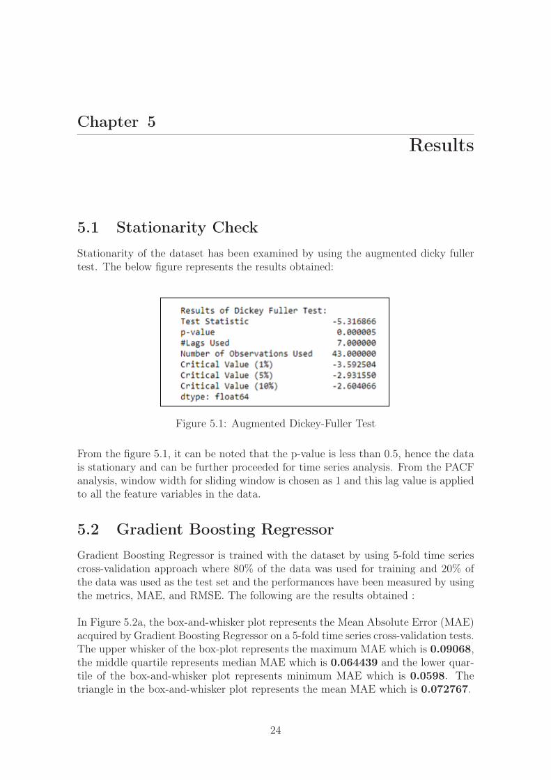
5.1 Stationarity CheckStationarity of the dataset has been examined by using the augmented dicky fullertest. The below figure represents the results obtained:

Figure 5.1: Augmented Dickey-Fuller Test

From the figure 5.1, it can be noted that the p-value is less than 0.5, hence the datais stationary and can be further proceeded for time series analysis. From the PACFanalysis, window width for sliding window is chosen as 1 and this lag value is appliedto all the feature variables in the data.

5.2 Gradient Boosting RegressorGradient Boosting Regressor is trained with the dataset by using 5-fold time seriescross-validation approach where 80% of the data was used for training and 20% ofthe data was used as the test set and the performances have been measured by usingthe metrics, MAE, and RMSE. The following are the results obtained :

In Figure 5.2a, the box-and-whisker plot represents the Mean Absolute Error (MAE)acquired by Gradient Boosting Regressor on a 5-fold time series cross-validation tests.The upper whisker of the box-plot represents the maximum MAE which is 0.09068,the middle quartile represents median MAE which is 0.064439 and the lower quar-tile of the box-and-whisker plot represents minimum MAE which is 0.0598. Thetriangle in the box-and-whisker plot represents the mean MAE which is 0.072767.

24

Chapter 5. Results 25

(a) MAE Box Plot (b) RMSE Box Plot

Figure 5.2: Gradient Boosting Error Box Plots

In Figure 5.2b, the box-and-whisker plot represents the Root Mean Squared Er-ror (RMSE) acquired by Gradient Boosting Regressor on a 5-fold time series cross-validation tests. The upper whisker of the box-plot represents the maximum RMSEwhich is 0.17933, the middle quartile represents median RMSE which is 0.10626and the lower quartile of the box-and-whisker plot represents minimum RMSE whichis 0.08634. The triangle in the box-and-whisker plot represents the mean RMSEwhich is 0.12661.

Figure 5.3 represents the actual and forecasted sales of target variant obtained usingthe Gradient boosting regression model where the orange line represents the actualvalues and blue line represents forecasted sales of the target variant interregionalhaul. This color notation is continued over the Figures 5.5,5.7,5.9.

Figure 5.3: Gradient Boosting Regression Prediction

5.3 Random Forest RegressorRandom Forest Regressor is trained with the dataset by using 5-fold time seriescross-validation approach where 80% of the data was used for training and 20% ofthe data was used as the test set and the performances have been measured by usingthe metrics MAE and RMSE.The following are the results obtained by the RandomForest Regressor:



Figure 5.4: Random Forest Regression Error Box Plots

In Figure 5.4a, the box-and-whisker plot represents the Mean Absolute Error (MAE)acquired by Random Forest Regressor on a 5-fold time series cross-validation tests.The upper whisker of the box-plot represents the maximum MAE which is 0.07096,the middle quartile represents median MAE which is 0.06315 and the lower quar-tile of the box-and-whisker plot represents minimum MAE which is 0.05283. Thetriangle in the box-and-whisker plot represents the mean MAE which is 0.062706.

In Figure 5.4b, the box-and-whisker plot represents the Mean Squared Error (RMSE)acquired by Random Forest Regressor on a 5-fold time series cross-validation tests.The upper whisker of the box-plot represents the maximum RMSE which is 0.1441,the middle quartile represents median RMSE which is 0.1064 and the lower quartileof the box-and-whisker plot represents minimum RMSE which is 0.07535. The trian-gle in the box-and-whisker plot represents the mean RMSE which is 0.10683. Figure5.5 represents the actual and forecasted sales of target variant transport segment-interregional haul obtained using the random forest regression model.

Figure 5.5: Random Forest Regressor Prediction

5.4 Support Vector Regressor (SVR)Support Vector Regressor is trained with the dataset by using 5-fold time seriescross-validation approach where 80% of the data was used for training and 20% of


the data was used as the test set and the performances have been measured by usingthe metrics MAE and RMSE. The following are the results obtained by the SupportVector Regressor:


Figure 5.6: Support Vector Regression Error Box Plots

In figure 5.6a, the box-and-whisker plot represents the Mean Absolute Error (MAE)acquired by Support Vector Regressor on a 5-fold time series cross-validation tests.The upper whisker of the box-plot represents the maximum MAE which is 0.08495,the middle quartile represents median MAE which is 0.06697 and the lower quar-tile of the box-and-whisker plot represents minimum MAE which is 0.06102. Thetriangle in the box-and-whisker plot represents the mean MAE which is 0.68752

In Figure 5.6b, the box-and-whisker plot represents the Root Mean Squared Er-ror(RMSE) acquired by Support Vector Regressor on a 5-fold time series cross-validation tests. The upper whisker of the box-plot represents the maximum RMSEwhich is 0.17254, the middle quartile represents median RMSE which is 0.09035and the lower quartile of the box-and-whisker plot represents minimum RMSE whichis 0.07127. The triangle in box-and-whisker plot represents the mean RMSE whichis 0.10188, figure 5.7 represents the actual and forecasted sales obtained using theSupport Vector regression model

Figure 5.7: Support Vector Regressor Prediction


5.5 Ridge RegressorRidge Regressor is trained with the dataset by using 5-fold time series cross-validationapproach where 80% of the data was used for training and 20% of the data was usedas the test set and the performances have been measured by using the metrics MAEand RMSE. The following are the results obtained by the Ridge Regressor:


Figure 5.8: Ridge Regression Error Box Plots

In figure 5.8a, the box-and-whisker plot represents the Mean Absolute Error (MAE)acquired by Ridge Regressor on a 5-fold time series cross-validation tests. The upperwhisker of the box-plot represents the maximum MAE which is 0.06814 the mid-dle quartile represents median MAE which is 0.05779 and the lower quartile of thebox-and-whisker plot represents minimum MAE which is 0.04508. The triangle inbox-and-whisker plot represents the mean MAE which is 0.058168.

Figure 5.8b, the box-and-whisker plot represents the RMSE acquired by Ridge Re-gressor on a 5-fold time series cross-validation tests. The upper whisker of the box-plot represents the maximum RMSE which is 0.1512, the middle quartile representsmedian RMSE which is 0.09114 and the lower quartile of the box-and-whisker plotrepresents minimum RMSE which is 0. 05572. The triangle in the box-and-whiskerplot represents the mean RMSE which is 0.09367, figure 5.9 represents the actualand forecasted sales of target variant obtained using the ridge regression model.

Figure 5.9: Ridge Regressor Prediction


5.6 Performance evaluation results

Algorithms Mean Absolute Error Root Mean Square Error

Ridge Regression 0.05816 0.09367

Support Vector Machine 0.06875 0.10188

Random Forest Regression 0.06270 0.10683

Gradient Bossting Regressor 0.07276 0.12661

Table 5.1: Comparison of performance evaluation results

From the table 5.1, Ridge Regression performed well with both the metrics MAE andRMSE, Ridge Regression has least error in forecasting the sales of truck componentswhen compared to the Support Vector Machine, Gradient Boosting regression andRandom Forest. The gradient boosting machine demonstrated the worst performancewith the highest error in both metrics.

Chapter 6Analysis and Discussion

6.1 Comparative study of Performance Metrics

6.1.1 Mean Absolute Error

Figure 6.1: Comparison of MAE obtained by regression models on 5-fold time seriesvalidation tests

Figure 6.1 represents the Mean Absolute error from the results of the predictions pro-duced by the Support Vector Regressor, Random Forest Regressor, Gradient Boost-ing Regressor and Ridge Regressor on 5-fold time series cross-validation tests. Fromthe figure, it can be seen that except in 2nd fold, Ridge regressor has least MAE inall the folds and thus can be said as a best-performed algorithm. Gradient boostinghas highest MAE and thus it can be said as worst performer.

6.1.2 Root Mean Squared Error

From figure 6.2, it can be noticed that Ridge Regression has shown spectacular overallperformance with the least RMSE and Gradient Boosting Regressor has shown worstperformance with the highest RMSE.

30

Chapter 6. Analysis and Discussion 31

Figure 6.2: Comparison of RMSE obtained by regression models on 5-fold time seriesvalidation tests

6.1.3 Average Mean Absolute Error

From figure 6.3, The average MAE acquired by the Ridge Regression across the 5-fold time series cross-validation is 0.058168, followed by the Random Forest Regressorwhich is 0.062706, thereafter SVR which is 0.068752 and finally Gradient BoostingRegressor which is 0.072767. From figure 6.3, it can said that Ridge Regression isthe best performer with the least error and Gradient boosting is the worst performerwith the highest error.

Figure 6.3: Comparison of Average MAE obtained by regression models on 5-foldtime series validation tests


6.1.4 Average Root Mean Square Error

From figure 6.4, The average RMSE acquired by the Ridge Regression across the5-fold time series cross-validation is 0.09367, followed by the SVR which is 0.101886,thereafter Random Forest Regressor which is 0.106836 and finally Gradient BoostingRegressor which is 0.12661. From figure 6.4, it can said that Ridge Regression isthe best performer with the least error and Gradient boosting is the worst performerwith the highest error.

Figure 6.4: Comparison of Average RMSE obtained by regression models on 5-foldtime series validation tests

6.2 Key AnalysisKey concepts behind the performance of algorithms are explored as follows:

• Ridge Regression has performed significantly well compared to the other mod-els. This may be because of the regularization approach where the variance isreduced at the cost of some bias initiation which makes it robust to outliersand overfitting.

• Support Vector Regression has performed surprisingly well compared to therandom forest and gradient boosting, this may be because of its generalizationcapability. Kernel function for the chosen parameters is set to ‘rbf’, other kernelfunctions like linear, radial may produce better results.

• Random Forest Regressor hasn’t shown good performance, this may be becauseof overfitting problem which may be preventing from generalizing the model.

• Gradient boosting produced bad results compared to others because of overfit-ting problem and Gradient Boosting Regressor is harder to tune compared toRandom Forest.


6.3 DiscussionRQ1: What are the suitable machine learning techniques for forecasting sales in thearea of finance?

Answer: Based on the results obtained from the Literature review, four machinelearning models namely Ridge Regressor, Support Vector Regressor, Random ForestRegressor, and Gradient boosting Regressor have been chosen for forecasting thesales.

RQ2: What are the performances of machine learning models for forecasting thesales of the core components of trucks based on the historical data?

Answer: Ridge Regression is the best suitable algorithm to forecast the sales oftruck components.In this experiment, Ridge Regression has least error in forecastingthe sales when compared to the Support Vector Machine, Random Forest, GradientBoosting regression. This is because of the regularization, where slack variablesare added to avoid over-fitting, Average RMSE across the 5-fold time series cross-validation is 0.09367 which is quite outstanding and Average MAE is 0.05779.Gradient Boosting has shown worst performance compared to the other algorithms,Average RMSE across the 5-fold time series cross-validation is 0.12661 which isworst and Average MAE is 0.07276. The performances of all the models have beendiscussed in Section 6.1

6.4 ContributionsAlthough there have been existing researches focusing on the sales forecasting byusing the statistical techniques in automotive industry, there has been no researchbased on developing the sales forecasting related to the truck components basedon the machine learning, which can be used for the sales team of any wide rangeof companies and organizations in the automotive industry. This thesis suggeststhat the machine learning approach can be used to get insights from the data and toforecast the sales of truck components. This approach can be further used to developadvanced forecasting tool which can able to forecast more precise forecasts.

6.5 Threats to ValidityThe concept of validity was formulated by Kelly, who expressed that a test is validif it measures what it claims to measure.

6.5.1 Internal Validity

Internal validity refers to the extent to which research was carried out [60], To over-come the threat of missing observations in the experiments, cloud backup is usedwhich consists of all the logs copies of the experiment


6.5.2 External Validity

External validity is the validity of applying the conclusions of a scientific studyoutside the context of that study [60]. This validity is attained by the data extractedfrom the sales database which has been used in this thesis study to evaluate thealgorithm and its performance. The risk of the particularity of variables is mitigatedby describing all the dependent variables of this study in such a way that they aresignificant in any general experimental settings.

6.5.3 Conclusion Validity

Conclusion validity refers to if the data used from the experiment and results arejustified and right [60]. This issue may be raised if there is no proper selectionof performance evaluation metrics can lead to an understanding of the size of therelationship between independent and dependent variables in the study. To avoid thisthreat multiple evaluation metrics have been used along with the proper structureof experimental setup and methodology.

6.6 Limitations• The study has been conducted on sales data which belonged to the truck sales of

Sweden region and it cannot be assured that the similar results will be obtainedfrom the study conducted on the sales data belonged to the other region as thesales may vary in other regions.

• Due to the unavailability of the company’s information like customer details,certain campaigns and discounts. They haven’t been included in data whichwould benefit in obtaining better forecasts.

Chapter 7Conclusions and Future Work

Sales forecasting is a pivotal part of the financial planning of business for any orga-nization. It can be said as a self-assessment tool which uses the statistics of the pastand the current sales in order to predict future performance. Sales forecasting playsan important role in optimising the truck sales process. Financial and Sales planningwith the help of the sales forecasts helps to get the information needed to predictthe revenue as well as the profit. Thus, in finding such solution for sales forecasts,machine learning algorithms such as Random Forest Regressor, Support Vector Re-gressor, Ridge Regressor, and Gradient Boosting Regressor have been evaluated onVolvo truck components sales data which can forecast the short term sales and helpthe organization in making the key decisions. After performing the various statis-tical tests and performance metrics, it is found that Ridge Regression is a suitablealgorithm in accordance to the chosen dataset and thus accomplishing the aim ofthis thesis.

7.1 Future WorkFuture work for this thesis involves comparing the performance evaluation results ofthe chosen regression techniques obtained from this thesis with the results obtainedfrom deep learning methods which could help the researchers in getting better trendsand results.

As mentioned earlier, due to the lack of information about external or environmentalvariables like promotions, discounts, etc. Such variables are not considered in themodeling and sales forecasting experiment. It is suggested to use the related data ofthe company for further research to obtain more accuracy.

35

Bibliography

[1] Chris Chatfield. Time-Series Forecasting. en. Chapman and Hall/CRC, Oct.2000. isbn: 978-0-429-12635-2. doi: 10.1201/9781420036206. url: https://www.taylorfrancis.com/books/9780429126352 (visited on 05/21/2019).

[2] Chi-Jie Lu, Tian-Shyug Lee, and Chia-Mei Lian. “Sales forecasting for com-puter wholesalers: A comparison of multivariate adaptive regression splines andartificial neural networks”. In: Decision Support Systems 54.1 (2012), pp. 584–596.

[3] James J Pao and Danielle S Sullivan. “Time Series Sales Forecasting”. In: FinalYear Project (2017).

[4] Mohit Gurnani et al. “Forecasting of sales by using fusion of machine learningtechniques”. In: 2017 International Conference on Data Management, Analyticsand Innovation (ICDMAI). IEEE, 2017, pp. 93–101.

[5] James E. Cox Jr and David G. Loomis. “Improving forecasting through text-books—A 25 year review”. In: International Journal of Forecasting 22.3 (2006),pp. 617–624.

[6] Michael Chui. “Artificial intelligence the next digital frontier?” In: McKinseyand Company Global Institute 47 (2017).

[7] Bruce Saunders. “A land development financial model”. In: (1990).

[8] Christoph Freudenthaler, Lars Schmidt-Thieme, and Steffen Rendle. “Bayesianfactorization machines”. In: (2011).

[9] A. Syntetos. “John T. Mentzer and Mark A. Moon, Sales forecasting manage-ment: A demand management approach , Sage Publications, Thousand Oaks,London (2005) ISBN 1-4129-0571-0 Softcover, 347 pages”. In: InternationalJournal of Forecasting 22.4 (2006), pp. 821–821.

[10] Bohdan M. Pavlyshenko. “Machine-Learning Models for Sales Time Series Fore-casting”. In: Data 4.1 (2019), p. 15.

[11] Chris Chatfield and Time-Series Forecasting. “Chapman & Hall”. In: CRC,London/Boca Raton (2001).

[12] Leo Breiman. “Random forests”. In: Machine learning 45.1 (2001), pp. 5–32.

[13] Jerome H. Friedman. “Greedy function approximation: a gradient boostingmachine”. In: Annals of statistics (2001), pp. 1189–1232.

[14] Jose Luis Blanco et al. “Artificial intelligence: Construction technology’s nextfrontier”. In: Building Economist, The September 2018 (2018), p. 8.

36

BIBLIOGRAPHY 37

[15] Ahmed Tealab. “Time Series Forecasting using Artificial Neural Networks Method-ologies: A Systematic Review”. In: Future Computing and Informatics Journal(2018).

[16] Jason Brownlee. Introduction to Time Series Forecasting with Python: How toPrepare Data and Develop Models to Predict the Future. Jason Brownlee, 2017.

[17] N. Alan Heckert. Statistical Engineering Division. en. Aug. 2010. url: https://www.nist.gov/itl/sed (visited on 05/21/2019).

[18] Andries P. Engelbrecht. Computational intelligence: an introduction. John Wi-ley & Sons, 2007.

[19] Leo Breiman. “Bagging predictors”. In: Machine learning 24.2 (1996), pp. 123–140.

[20] Juan Huo, Tingting Shi, and Jing Chang. “Comparison of Random Forest andSVM for electrical short-term load forecast with different data sources”. In:2016 7th IEEE International Conference on Software Engineering and ServiceScience (ICSESS). IEEE, 2016, pp. 1077–1080.

[21] Turi. Random Forest Regression | Turi Machine Learning Platform User Guide.url: https://turi.com/learn/userguide/supervised-learning/random_forest_regression.html (visited on 05/21/2019).

[22] Debasish Basak, Srimanta Pal, and Dipak Chandra Patranabis. “Support vec-tor regression”. In: Neural Information Processing-Letters and Reviews 11.10(2007), pp. 203–224.

[23] Vladimir Vapnik, Steven E. Golowich, and Alex J. Smola. “Support vectormethod for function approximation, regression estimation and signal process-ing”. In: Advances in neural information processing systems. 1997, pp. 281–287.

[24] Saed Sayad. Real time data mining. Self-Help Publishers Cambridge, 2011.

[25] J. Al-Jararha. “New approaches for choosing the ridge parameters”. In: HacettepeJournal of Mathematics and Statistics 47.6 (2016), pp. 1625–1633.

[26] scikit-learn: machine learning in Python — scikit-learn 0.21.1 documentation.url: https://scikit-learn.org/stable/ (visited on 05/21/2019).

[27] Boosted Trees Regression | Turi Machine Learning Platform User Guide. url:https://turi.com/learn/userguide/supervised- learning/boosted_trees_regression.html (visited on 05/21/2019).

[28] NumPy — NumPy. url: http://www.numpy.org/ (visited on 05/21/2019).

[29] GE Box et al. Time series analysis, control, and forecasting . Hoboken. 2015.

[30] Mohit Gurnani et al. “Forecasting of sales by using fusion of machine learningtechniques”. In: 2017 International Conference on Data Management, Analyticsand Innovation (ICDMAI). IEEE. 2017, pp. 93–101.

[31] Peter R Winters. “Forecasting sales by exponentially weighted moving aver-ages”. In: Management science 6.3 (1960), pp. 324–342.

BIBLIOGRAPHY 38

[32] Francis EH Tay and Lijuan Cao. “Application of support vector machines infinancial time series forecasting”. In: omega 29.4 (2001), pp. 309–317.

[33] K-R Müller et al. “Predicting time series with support vector machines”. In: In-ternational Conference on Artificial Neural Networks. Springer. 1997, pp. 999–1004.

[34] Mariana Rafaela Oliveira and Luis Torgo. “Ensembles for time series forecast-ing”. In: (2014).

[35] Cheng Cheng, Wei Xu, and Jiajia Wang. “A comparison of ensemble methodsin financial market prediction”. In: 2012 Fifth International Joint Conferenceon Computational Sciences and Optimization. IEEE, 2012, pp. 755–759.

[36] L. I. N. Feng-Jenq. “Adding EMD Process and Filtering Analysis to EnhancePerformances of ARIMA Model When Time Series Is Measurement Data”. In:Romanian Journal of Economic Forecasting 18.2 (2015), p. 92.

[37] Donglin Wang and Yajie Li. “A novel nonlinear RBF neural network ensemblemodel for financial time series forecasting”. In: Third International Workshopon Advanced Computational Intelligence. IEEE, 2010, pp. 86–90.

[38] Mohammed A Al-Gunaid et al. “Time series analysis sales of sowing cropsbased on machine learning methods”. In: 2018 9th International Conferenceon Information, Intelligence, Systems and Applications (IISA). IEEE. 2018,pp. 1–6.

[39] Andreas Zell. Simulation neuronaler netze. Vol. 1. 5.3. Addison-Wesley Bonn,1994.

[40] Guolin Ke et al. “Lightgbm: A highly efficient gradient boosting decision tree”.In: Advances in Neural Information Processing Systems. 2017, pp. 3146–3154.

[41] R Samsudin, A Shabri, and P Saad. “A comparison of time series forecastingusing support vector machine and artificial neural network model”. In: Journalof applied sciences 10.11 (2010), pp. 950–958.

[42] Yaohui Bai et al. “Forecasting financial time series with ensemble learning”. In:2010 International Symposium on Intelligent Signal Processing and Communi-cation Systems. IEEE. 2010, pp. 1–4.

[43] Akshay Krishna et al. “Sales-forecasting of Retail Stores using Machine Learn-ing Techniques”. In: 2018 3rd International Conference on Computational Sys-tems and Information Technology for Sustainable Solutions (CSITSS). IEEE.2018, pp. 160–166.

[44] Python Data Analysis Library — pandas: Python Data Analysis Library. url:https://pandas.pydata.org/ (visited on 05/21/2019).

[45] Matplotlib: Python plotting — Matplotlib 3.1.0 documentation. url: https://matplotlib.org/ (visited on 05/21/2019).

[46] seaborn: statistical data visualization — seaborn 0.9.0 documentation. url:https://seaborn.pydata.org/ (visited on 05/21/2019).

[47] Project Jupyter. url: https://www.jupyter.org (visited on 05/21/2019).

BIBLIOGRAPHY 39

[48] Long Short-Term Memory Networks With Python. en-US. url: https : / /machinelearningmastery.com/lstms-with-python/ (visited on 05/21/2019).

[49] Kedar Potdar, Taher S. Pardawala, and Chinmay D. Pai. “A comparative studyof categorical variable encoding techniques for neural network classifiers”. In:International Journal of Computer Applications 175.4 (2017), pp. 7–9.

[50] Jason Brownlee. Time Series Forecasting as Supervised Learning. May 2017.url: https://machinelearningmastery.com/time-series-forecasting-supervised-learning/.

[51] Agus Widodo, Indra Budi, and Belawati Widjaja. “Automatic lag selection intime series forecasting using multiple kernel learning”. In: International Journalof Machine Learning and Cybernetics 7.1 (2016), pp. 95–110.

[52] David A. Dickey and Wayne A. Fuller. “Distribution of the estimators for au-toregressive time series with a unit root”. In: Journal of the American statisticalassociation 74.366a (1979), pp. 427–431.

[53] Time Series Forecasting as Supervised Learning. url: https://machinelearningmastery.com/time-series-forecasting-supervised-learning/ (visited on 05/21/2019).

[54] G. Udny Yule. “Why do we sometimes get nonsense-correlations between Time-Series?–a study in sampling and the nature of time-series”. In: Journal of theroyal statistical society 89.1 (1926), pp. 1–63.

[55] M. Kendall and Jean D. Gibbons. “Rank correlation methods edward arnold”.In: A division of Hodder & Stoughton, A Charles Griffin title, London (1990),pp. 29–50.

[56] Erich L. Lehmann and George Casella. Theory of point estimation. SpringerScience & Business Media, 2006.

[57] Georgios Drakos. How to select the Right Evaluation Metric for Machine Learn-ing Models: Part 2 Regression Metrics. Sept. 2018. url: https://towardsdatascience.com / how - to - select - the - right - evaluation - metric - for - machine -learning-models-part-2-regression-metrics-d4a1a9ba3d74 (visited on05/21/2019).

[58] Rob J. Hyndman and George Athanasopoulos. Forecasting: principles and prac-tice. OTexts, 2018.

[59] Christoph Bergmeir and José M Benıtez. “On the use of cross-validation fortime series predictor evaluation”. In: Information Sciences 191 (2012), pp. 192–213.

[60] Barbara Ann Kitchenham, David Budgen, and Pearl Brereton. Evidence-basedsoftware engineering and systematic reviews. Vol. 4. CRC press, 2015.

Faculty of Computing, Blekinge Institute of Technology, 371 79 Karlskrona, Sweden

machine learning approach for forecasting the sales of

Documents