machine learning approaches to strongly correlated spin...

Machine learning approaches to strongly correlated

spin systems

Tom Vieijra

Ghent University

Department of Physics and AstronomyTheoretical Nuclear and Statistical Physics

Machine learning approaches to stronglycorrelated spin systems

Tom Vieijra

1. Promotor Prof. Dr. Jan RyckebuschDepartment of Physics and AstronomyGhent University

2. Supervisor Dr. Jannes NysDepartment of Physics and AstronomyGhent University

3. Supervisor Corneel CasertDepartment of Physics and AstronomyGhent University

Thesis submitted in partial fulfillment for the degreeof Master of Science in Physics and Astronomy

May 31, 2018

Tom Vieijra

Machine learning approaches to strongly correlated spin systems

Documentation, May 31, 2018

Reviewers: Prof. Dr. Jan Ryckebusch, Dr. Jannes Nys, Prof. Dr. Jutho Haegeman and Prof.

Dr. Wesley De Neve

Supervisors: Prof. Dr. Jan Ryckebusch, Dr. Jannes Nys and Corneel Casert

Ghent University

Theoretical Nuclear and Statistical Physics

Department of Physics and Astronomy

Proeftuinstraat 86, building N3

B-9000 Ghent

Abstract

Understanding systems of many degrees of freedom forms one of the most complexproblems in physics. These systems can be described by only taking their macroscopicproperties into account (thermodynamics). Another way of getting insight in thesesystems is examining how the individual degrees of freedom give rise to the macro-scopic properties. This branch of physics is called many-body physics. Finding howthe macroscopic properties arise from the collection of individual degrees of freedomrequires a way to connect microscopic and macroscopic properties of the systemunder study. How to make this connection is formally described by statistical physicsand quantum many-body physics. However, making this connection in practice oftenrequires approximations to the applicable physical laws and a substantial amountof computation. Numerous approximation methods have been developed in thephysics community. Recently, a new toolbox was added to the body of approximationmethods, namely machine learning. Machine learning techniques have the abilityto make the connection between data and abstract concepts in a scalable way. Inessence they are able to make the connection between microscopic variables (e.g.pixels in an image) and macroscopic concepts (e.g. the object contained in theimage).

In this thesis, the connection between many-body physics and machine learning isfirst examined (chapters 1, 2 and 3). After giving the motivation to use machinelearning techniques for problems in many-body physics, we proceed in chapter 4 witha specific application of it on the problem of finding the ground state of quantummany-body spin systems. Specifically, we model the ground-state wave function ofthe transverse field Ising and antiferromagnetic Heisenberg models, both in oneand two spatial dimensions. This is done with the aid of a restricted Boltzmannmachine (which is a stochastic neural network) to model the probability amplitudesin the expansion of the wave function. We examine the accuracy and the scalingof the technique, as well as the internal representation of the restricted Boltzmannmachine and its relation to physical quantities. In chapter 5, we examine whetherthe restricted Boltzmann machine is capable of representing ground-state wavefunctions at or near a quantum phase transition. The motivation to study this is thefact that the wave function contains the largest amount of non-trivial correlationsat the transition point between two phases, which makes it significantly harder to

v

describe. We perform a finite-size scaling analysis for the one-dimensional transversefield Ising system to determine the critical point and the critical exponents, andexamine different relevant observables of the macroscopic system (e.g. the Bindercumulant and the correlation functions). We also compare our results with theresults of other techniques available in literature.

vi

Acknowledgement

Allereerst zou ik Jannes en professor Ryckebusch willen bedanken voor de opportu-niteit die jullie mij gegeven hebben om deze thesis te maken. Jullie enthousiasmeover dit onderwerp gaf mij telkens een boost om verder te werken aan hetgeenin de volgende bladzijden te lezen staat. Bedankt voor jullie kennis van zaken enconstructieve feedback op mijn werk.

Andres and Corneel, thank you for helping me with the servers and other computer-related problems, and the coffee afterwards. Also thanks to the other people at INWfor bumping into each other and the interesting things you had to say.

Mede-thesisstudenten, een welgemeende dankjulliewel voor de lunches, de dilemma’sen het kletsen als pauze.

Hilde Van Oostenryck en Hilde Verheijen van het Xaveriuscollege in Borgerhout,bedankt voor jullie enthousiasme voor wiskunde en wetenschappen. Zonder julliehad ik hier nooit gestaan. Jullie speelden een ongelooflijk belangrijke rol in hetkiezen van deze studierichting, waar ik geen moment spijt van heb gehad.

Vrienden van ’t stad, bedankt voor de koffie en het luisteren naar mijn oneindigestroom aan fysica-praatjes.

Mama, papa en Michiel, bedankt voor jullie vertrouwen, de kansen die jullie mijgegeven hebben en het fietsen.

Annelies, bedankt om er altijd voor mij te zijn en mijn doemscenario’s telkens weerte ontkrachten. Je positivisme bracht me telkens weer op het juiste spoor. Zonderjou was ik waarschijnlijk al lang ergens gestrand in een onmetelijk leeg veld of opeen verlaten eiland.

vii

Contents

1 Introduction to many-body physics 11.1 Classical statistical physics . . . . . . . . . . . . . . . . . . . . . . . . 21.2 Quantum many-body physics . . . . . . . . . . . . . . . . . . . . . . 31.3 Emergence in many-body physics . . . . . . . . . . . . . . . . . . . . 61.4 Quantum statistical physics . . . . . . . . . . . . . . . . . . . . . . . 8

2 Introduction to machine learning 132.1 The machine learning strategy . . . . . . . . . . . . . . . . . . . . . . 142.2 Classification of machine learning approaches . . . . . . . . . . . . . 162.3 Some notable machine learning algorithms . . . . . . . . . . . . . . . 17

2.3.1 PCA and t-SNE . . . . . . . . . . . . . . . . . . . . . . . . . . 172.3.2 Support vector machines . . . . . . . . . . . . . . . . . . . . . 182.3.3 Neural networks . . . . . . . . . . . . . . . . . . . . . . . . . 192.3.4 Generative adversarial networks . . . . . . . . . . . . . . . . 25

3 Combining many-body physics and machine learning 273.1 Physics in machine learning . . . . . . . . . . . . . . . . . . . . . . . 283.2 Machine learning in physics . . . . . . . . . . . . . . . . . . . . . . . 31

3.2.1 Machine learning for model selection . . . . . . . . . . . . . . 313.2.2 Machine learning for improvement of simulations in physics . 323.2.3 Machine learning to detect high-level features in complex

systems . . . . . . . . . . . . . . . . . . . . . . . . . . . . . . 34

4 Modelling ground states of quantum systems with restricted Boltzmann machines 394.1 Variational ansatz . . . . . . . . . . . . . . . . . . . . . . . . . . . . . 39

4.1.1 RBM representation of wave functions . . . . . . . . . . . . . 394.1.2 Implementing symmetries . . . . . . . . . . . . . . . . . . . . 41

4.2 Optimizing the wave function . . . . . . . . . . . . . . . . . . . . . . 444.2.1 Initializing the wave function . . . . . . . . . . . . . . . . . . 444.2.2 Update of the parameters . . . . . . . . . . . . . . . . . . . . 454.2.3 Convergence criteria . . . . . . . . . . . . . . . . . . . . . . . 524.2.4 Summary of the algorithm used to determine ground states . 53

4.3 Theoretical properties and other methods . . . . . . . . . . . . . . . 544.3.1 Theoretical properties . . . . . . . . . . . . . . . . . . . . . . 54

ix

4.3.2 Other methods . . . . . . . . . . . . . . . . . . . . . . . . . . 554.4 Quantum spin systems . . . . . . . . . . . . . . . . . . . . . . . . . . 59

4.4.1 Transverse field Ising model . . . . . . . . . . . . . . . . . . . 594.4.2 Antiferromagnetic Heisenberg model . . . . . . . . . . . . . . 61

4.5 Results . . . . . . . . . . . . . . . . . . . . . . . . . . . . . . . . . . . 624.5.1 Ground-state energy . . . . . . . . . . . . . . . . . . . . . . . 624.5.2 Scaling . . . . . . . . . . . . . . . . . . . . . . . . . . . . . . 664.5.3 Energy fluctuations . . . . . . . . . . . . . . . . . . . . . . . . 684.5.4 Comparison with literature . . . . . . . . . . . . . . . . . . . 684.5.5 RBM representation as a function of iteration step . . . . . . . 704.5.6 Weight histograms . . . . . . . . . . . . . . . . . . . . . . . . 744.5.7 Correlations . . . . . . . . . . . . . . . . . . . . . . . . . . . . 76

5 Finite-size scaling for the Transverse Field Ising model 815.1 The finite-size scaling method . . . . . . . . . . . . . . . . . . . . . . 815.2 Finite-size scaling results with restricted Boltzmann machines . . . . 85

5.2.1 Magnetization histograms . . . . . . . . . . . . . . . . . . . . 865.2.2 Binder cumulant . . . . . . . . . . . . . . . . . . . . . . . . . 875.2.3 Order parameter . . . . . . . . . . . . . . . . . . . . . . . . . 905.2.4 Order parameter susceptibility . . . . . . . . . . . . . . . . . 915.2.5 Integral of correlation function . . . . . . . . . . . . . . . . . 925.2.6 Comparison with other work . . . . . . . . . . . . . . . . . . 925.2.7 Conclusion . . . . . . . . . . . . . . . . . . . . . . . . . . . . 96

6 Conclusion and outlook 976.1 Conclusion . . . . . . . . . . . . . . . . . . . . . . . . . . . . . . . . 976.2 Outlook . . . . . . . . . . . . . . . . . . . . . . . . . . . . . . . . . . 99

Nederlandse samenvatting 101

Science popularization 103

Bibliography 105

List of symbols 113

List of Figures 115

List of Tables 121

x

1Introduction to many-body physics

Many-body physics deals with physical problems with a large amount of interactingdegrees of freedom. In this definition, large can have different meanings, rangingfrom the amount of electrons present in atoms (∼ 10− 100), the amount of atomspresent in nanomaterials (∼ 106) or the amount of atoms involved in macroscopicsamples of matter (∼ 1023). The physical problem is to connect the properties ofthe microscopic degrees of freedom to the macroscopic behaviour of the collective.Solving these problems is important both from a theoretical and experimental pointof view. On the theoretical side, one is interested in the underlying mechanisms thatgenerate the macroscopic properties of systems of many interacting constituents.From an experimental point of view, one uses the connection between microscopicand macroscopic properties to develop and engineer new materials with valuableand desirable characteristics.

Finding how the interactions between the degrees of freedom give rise to macroscopicproperties is a challenging problem. The interactions between the constituentsgenerate complexity in the system. This means that the physics cannot be solvedby considering the behaviour of one degree of freedom and treating the systemas a collection of them, independent of each other. While the occurrence of theseso-called correlations makes these systems hard to deal with, it is also the reasonfor their elusive properties. Examples of emergent properties are long-range order,topological properties and phase transitions. Another way to coin this is the famousphrase: “The whole is more than the sum of its parts”.

The many-body problem can be approximately solved with a number of techniques.For classical microscopic degrees of freedom, statistical physics can be used.1 Forquantum mechanical degrees of freedom, quantum statistical physics can be usedfor problems at finite temperature and quantum many-body physics can be used forproblems at zero temperature. In this work, we use tools from both statistical andquantum many-body physics.

1Statistical physics can also be used to describe quantum mechanical systems, as long as the eigen-spectrum of the energy is known.

1

1.1 Classical statistical physics

Statistical physics describes systems with many degrees of freedom from a statisticalpoint of view. To this end, one defines a probability distribution over the possiblemicroscopic configurations of the system. This probability distribution can then beused to find the macroscopic properties of the system as expectation values over theprobability distribution. To define the probability distribution, one must define someproperties of the macroscopic system. For example, the system can be viewed atconstant temperature T or at constant energy E. Other variables that determine thebehaviour of the system are pressure P or volume V , and the number of degrees offreedom N or the chemical potential µ. These variables are called control variables;they represent the conditions under which the system is studied. The combinationof the control variables defines an ensemble, for which one can find the probabilitydistribution. A common ensemble is the (N,V, T ), or canonical, ensemble where thenumber of degrees of freedom, the volume and the temperature are kept constant.

A common example of a non-trivial system in statistical physics is the Ising model,which is a model for (ferro)magnetism. The degrees of freedom are N spins{si}i=1...N which are spatially localized on lattice sites. The spins can have spinprojections siz = −1/2 or siz = 1/2 in the sz-basis. The microscopic configurationsof the system are thus the different combinations of the spin values in the system.For this system the control variables are (N,h‖, T ), where h‖ is the magnetic fieldlongitudinal to the z-direction. To define the probability distribution for this system,we define an energy function. In the Ising model, this is defined as [1]

E(S) = −j∑

〈i,k〉

sizskz − h‖

N∑

i=1

siz, (1.1)

where, S ≡ {siz}i=1...N is a specific configuration of the spin projections and∑〈i,k〉 is

a sum over all pairs of nearest neighbours. Further, j is the magnitude of the nearestneighbour interactions, where j > 0 leads to ferromagnetic interactions (the systemhas a lower energy when spins are aligned) and j < 0 leads to antiferromagneticinteractions (the system has a lower energy when spins are antialigned). Thefunction of Eq. (1.1) defines an energy value for all the different configurations ofthe system. The probability in the (N,h‖, T ) ensemble for a spin configuration S isthen given as

p(N,h‖,T )(S) =exp

(−E(S)kBT

)

∑S′ exp

(−E(S′)

kBT

) =exp

(−E(S)

kT

)

Z(N,h‖, T ). (1.2)

2 Chapter 1 Introduction to many-body physics

Here, kB is the Boltzmann constant and Z is the partition function. The partitionfunction is central for statistical physics as many properties of the system can bederived from it. Unfortunately, the sum over the different configurations is oftenintractable and can only be computed exactly in a very limited amount of cases. Tosolve this, one needs to resort to computational approaches such as Markov ChainMonte Carlo [2] or approximating techniques such as cluster expansions [3].

A nice feature of statistical physics is that it can be used outside of physics forproblems with many interacting degrees of freedom. Examples are social systems[4], flocking [5], epidemiology [6] and notably machine learning [7].

1.2 Quantum many-body physics

Quantum mechanics is the theory which describes physical degrees of freedom onmicroscopic scales. Examples are the physics of atoms and molecules, and thephysics of subatomic particles. Quantum many-body physics seeks to compute thezero-temperature properties of quantum mechanical systems with many degrees offreedom, defined by a Hamiltonian H, at zero temperature (see for example [8]).The properties of quantum mechanical systems are encoded in states |ψ〉, living ina Hilbert space H. These states are conventionally called quantum states or wavefunctions. For a system of N distinguishable2 degrees of freedom (e.g. when theyare spatially localized on lattice sites), the Hilbert space of the system is the directproduct of the Hilbert spaces of the separate degrees of freedom:

H = H1 ⊗H2 ⊗ ...⊗HN , (1.3)

whereHi is the Hilbert space of the i-th degree of freedom. This shows that quantummechanical problems with many degrees of freedom suffer from the curse of dimen-sionality, as the dimension D of the many-body Hilbert space scales exponentiallywith N as

D = dim(H) =N∏

i=1

dim(Hi). (1.4)

In principle, the non-relativistic many-body problem is fully solved upon integratingthe time independent Schrödinger equation (for systems where H is not explicitlytime dependent) for the energy eigenvalues and eigenfunctions

H |ψn〉 = En |ψn〉 , (1.5)

2For indistinguishable degrees of freedom, there are certain relations the states should obey (e.g. thestates need to be antisymmetric under exchange of two degrees of freedom in fermionic systems),making the effective size of the Hilbert space of possible physical states smaller. In this work, weonly work with distinguishable degrees of freedom.

1.2 Quantum many-body physics 3

where En is the energy eigenvalue belonging to the n-th eigenfunction |ψn〉. Afterchoosing an appropriate basis {|i〉}i=1...D, the eigenvalue equation reduces to amatrix diagonalization problem of the Hamiltonian matrix H, which is defined as

[H]ij = 〈i|H|j〉 . (1.6)

However, the dimension of the matrix grows exponentially with the number ofdegrees of freedom. The dimension of the matrix equals the dimension of the Hilbertspace, which scales as Eq. (1.4). Diagonalizing a matrix with dimension D generallyscales as O(D3) [9]. Unless the matrix has some property which speeds up thediagonalization algorithm (diagonal, block-diagonal, very sparse, ...), one has toresort to approximation techniques such as variational wave functions [2], quantumMonte Carlo [10] or perturbation theory [8].

In this thesis, we will work with quantum spin systems on a lattice, where the numberof degrees of freedom N is fixed. For spins with total spin s = 1/2, the Hilbert spaceof a single degree of freedom has dimension 2. We can define the Hilbert space interms of the eigenstates of the sz-operator (which is the spin-projection operator onthe z-axis) , denoted as

∣∣∣∣sz = +1

2

⟩=

(1

0

),

∣∣∣∣sz = −1

2

⟩=

(0

1

). (1.7)

The spin operators in the three Cartesian directions are related to the Pauli matricesvia sx = 1

2σx, sy = 12σy, sz = 1

2σz. In the basis defined in Eq. (1.7), the Pauli-operators are defined as

σx =

(0 1

1 0

), σy =

(0 −ii 0

), σz =

(1 0

0 −1

). (1.8)

These operators satisfy the commutation relations

[σa, σb] = 2iεabcσc, (1.9)

where εabc is the Levi-Civita tensor. The anti-commutation relations for the Pauli-operators are

{σa, σb} = 2δabI , (1.10)

where δab is the Kronecker delta and I is the identity operator. From the definitionof σz in Eq. (1.8), we see that the states in Eq. (1.7) have eigenvalues +1 and −1

respectively. Due to this fact, the first state in Eq. (1.7) is called the spin up state |↑〉and the second one the spin down state |↓〉. A state in a many-body Hilbert spacecan be written as a direct product of the states in the Hilbert spaces of the individual


degrees of freedom. For a {si = 1/2}i=1...N many-body spin system, we can define abasis for its Hilbert space as the direct product of the basis states in Eq. (1.7)

|s1zs

2z...s

Nz 〉 = |s1

z〉 ⊗ |s2z〉 ⊗ ...⊗ |sNz 〉 , (1.11)

where |siz〉 is the basis state of the i-th degree of freedom. In this work, Hamiltoniansoperating on spin degrees of freedom will be written in terms of the Pauli matrices.The transition between spin operators and Pauli matrices will not be given explicitly.The constant factors relating the Pauli matrices to the spin operators will be eitherdecimated via a rescaling of the energy or absorbed in prefactors. For example

H = cs1xs

2x → cσ1

xσ2x, (1.12)

where c = c/4. When writing an operator depending on a single degree of freedomi, for example six in Eq. (1.12), we implicitly mean that it only operates non-triviallyon degree of freedom i, i.e.

six ≡ I1 ⊗ ...⊗ Ii−1 ⊗ six ⊗ Ii+1 ⊗ ...⊗ IN , (1.13)

where Ij is the unit operator acting on degree of freedom j.

Quantum many-body physics shares many properties with statistical physics. Toshow this, we will examine the transverse field Ising model (TFI). This model isdefined in the same way as the Ising model of Eq. (1.1), with the addition of atransverse magnetic field and no magnetic field parallel to the spins. The describedsituation can be modelled with the following Hamiltonian

H = Hz + Hx = −j∑

〈i,k〉

σizσkz − h

N∑

i=1

σix. (1.14)

Here, σiz and σix are the Pauli matrices of Eq. (1.7) operating only on the spin stateof the i-th spin. Further, j is the magnitude of the nearest-neighbour interactionsand h is the magnitude of the external transverse field. We will denote the ratio of hand j as g

g ≡ h

j. (1.15)

Note the resemblance with the classical Ising model. One can raise the questionof what a quantum mechanical problem at zero temperature has to do with aclassical problem at non-zero temperature, apart from the fact that many degreesof freedom are involved. One way to connect these two areas of physics is withthe concept of uncertainty. We noticed in section 1.1 that temperature introducesuncertainty in Nature due to the fact that it introduces a probability distributionfor the different configurations. Another mechanism to generate uncertainty is

1.2 Quantum many-body physics 5

superposition in quantum mechanics. Superposition means that, given a specificbasis for the problem at hand, the quantum states which solve the Schrödingerequation are a linear combination of these basis states. For example, in the TFIproblem we can choose the eigenbasis of the σz-operators of Eq. (1.11), yielding asa basis the configurations consisting of all possible combinations of up and downspins. Superposition arises when the Hamiltonian contains contributions which donot commute with each other. In the TFI model, this is the case because [Hz, Hx] 6= 0

due to Eq. (1.9). A consequence of superposition is that expectation values of a givenobservable, for example the magnetization in the z-direction, become weighted sumsfor the different basis functions. This is just like expectation values in statisticalphysics are weighted sums of the observable for the different configurations. While instatistical physics the uncertainty is introduced by the surroundings of the system, theuncertainty in quantum mechanics is an inherent part of the theory. This parallelismis striking. Differences remain as both settings have additional features not found inthe other, such as entanglement in quantum mechanics and the ergodic hypothesisin statistical physics.

1.3 Emergence in many-body physics

T < Tc

order

T ≈ Tc

order/disorder

T > Tc

disorder

Fig. 1.1: Depiction of the phases in the 2D classical Ising model of Eq. (1.1) (with h‖ = 0)and the transition between them. The spins on the square lattice are depicted asblack or white squares, where black squares have siz = 1/2 and white squares havesiz = −1/2. The phase transition occurs when the temperature reaches Tc.

As stated in the beginning of this chapter, many-body systems have some featureswhich are not found in the physics of the individual constituents. This property ofmany-body physics is often referred to as emergence. For example, phase transitionsare one of the most notable manifestations of emergent properties of physicalsystems. The emergence of phases and transition between them in a system of manyinteracting degrees of freedom is a feature that cannot be understood starting fromthe individual degrees of freedom. It is the result of the subtle interplay between twomechanisms with opposing effects which is referred to as frustration. In statistical


g < gc

order

g ≈ gc

order/disorder

g > gc

disorder

Fig. 1.2: Schematic representation of the phases of the 1D Transverse field Ising model of Eq.(1.14) and the transition between them. The black bars denote spins in state |↑〉and the white bars spins in state |↓〉. The transition occurs when g = 1 (see section4.4.1). Note the qualitative resemblance with figure 1.1.

physics, the equilibrium state of the system is defined by the minimization of thefree energy F

F = E − TS. (1.16)

In this equation, E is the energy, T is the temperature and S is the entropy. Minimiz-ing the free energy comes down to energy minimization and entropy maximization.These two operations have an influence on each other as energy minimizationtends to also minimize the entropy and energy maximization tends to maximizethe entropy. The upshot is a state of the system in between these two extremes,governed by the value of the temperature. When the temperature is low, energyminimization tends to play a more important role. In the Ising system introduced inEq. (1.14), this boils down to a state where almost all the spins are aligned, i.e. anordered state. When the temperature is high, the entropy maximization becomes thedominant contribution to F and therefore a disordered state is favoured. In betweenthese extremes, the system undergoes a transition. The transition described here isdepicted in figure 1.1

In the spirit of the relation between statistical physics and quantum many-bodyphysics, phase transitions can also be found in (the ground state of) quantum many-body systems. Under these circumstances, energy minimization leads to frustration.Note that the Hamiltonian of the transverse field Ising model of Eq. (1.14) consists oftwo distinct terms. Suppose that h = 0, we see easily that the state which minimizesthe Hz-part of the energy is the state with all spins aligned. Suppose now thath 6= 0. The term involving σx-operators does not commute with the term involvingσz-operators. The quantum state which minimizes the Hz-part of the Hamiltonian isnot an eigenstate of the Hx-part of the Hamiltonian. It follows that this state is notthe ground state because the ground state is an eigenstate of the full Hamiltonian.The ground state is thus not a state which minimizes both parts of the Hamiltonianindependently. This generates frustration as the true ground state compromisesbetween opposing terms in the Hamiltonian. Unlike in the classical case, it is nottemperature which generates transitions between the two phases, but rather the

1.3 Emergence in many-body physics 7

strength of the transverse field h. When h tends to zero, the resulting state will lieclose to the eigenstate of the Hz-part of the Hamiltonian, i.e. with all spins up ordown. When h is large, the resulting state will lie close to the eigenstates of theHx-part, i.e. states with zero magnetization. In between, a phase transition occurs.The phase transition in the 1D transverse field Ising model is schematically depictedin figure 1.2.

1.4 Quantum statistical physics

In section 1.1, we introduced statistical physics for systems for which the energyvalues of the different configurations are known. This enables one to solve tempera-ture dependent many-body problems. In section 1.2, quantum mechanical problemswith many interacting degrees of freedom were introduced. However, the discussionwas limited to physics at zero temperature. Combining both areas of physics leadsto quantum statistical physics, where temperature dependent quantum many-bodyproblems are treated. To develop quantum statistical physics, it is necessary toexpress a classical probability distribution over a collection of quantum states. Thisis most easily done in the density operator formalism of quantum mechanics (seefor example [11]). A density operator ρ is a non-negative operator with trace one,defined on the Hilbert space of the system. This operator describes the state of thesystem. For example, the density operator of a single state |Ψ〉 is

ρ = |Ψ〉〈Ψ| . (1.17)

The density operator allows to represent both single states and probability distribu-tions over multiple states with the same object. The expectation value of an operatorA is given by

Tr(Aρ). (1.18)

A system with Hamiltonian H in the (N,V, T ) ensemble is defined by the densityoperator [12]

ρ(N,V,T ) =exp

(− HkT

)

Tr(

exp(− HkT

)) =exp

(− HkT

)

Z(N,V, T ). (1.19)

Here, the exponential of an operator A is defined as

exp(A) =

∞∑

i=0

1

i!Ai, (1.20)


where A0 = I. The denominator of Eq. (1.19) (Z(N,V, T )) is called the partitionfunction, analogously to Eq. (1.2). Note that Eq. (1.19) reduces to Eq. (1.2) whenthe Hamiltonian is represented in its eigenbasis.

In section 1.2, a qualitative relation between statistical physics at non-zero tem-perature and quantum many-body physics at zero temperature was given. Thisrelationship can be made more rigorous using quantum statistical physics [12, 13].Considering the 1D transverse field Ising model of Eq. (1.14), the partition functionfor this Hamiltonian can be written down:

ZTFI = Tr(exp(−βHTFI)), (1.21)

where β = 1/kBT . Calculating this trace is non-trivial as H is not diagonal. Theenergy of the ground state Egs of this system corresponds with

Egs = limT→0−kBT ln (ZTFI) . (1.22)

We introduce the dimensionless quantity

m ≡ h/kBT = hβ, (1.23)

where h is the coupling of the transverse field in Eq. (1.14). The limit T → 0

corresponds to m→∞. In the following, we restrict m to integer values. This hasno effect on the analysis because the limit of m to infinity is taken.

Using Eq. (1.23) in Eq. (1.22) yields

Egs = limm→∞

− hm

ln(

Tr(

exp(−mhHTFI

))). (1.24)

The operatorexp

(−mhHTFI

)(1.25)

can be approximated by applying the Suzuki-Trotter decomposition [14],

exp

(∑

i

Ai

)= lim

n→∞

(∏

i

exp(Ai/n)

)n. (1.26)

By writing the argument of the exponential in Eq. (1.25) as a sum over m identicalterms −HTFI/h, applying the Suzuki-Trotter decomposition on Eq. (1.24) yields

Egs = limm→∞

limn→∞

− hm

ln

(Tr

((m∏

i=1

exp

(− 1

hnHTFI

))n)). (1.27)

1.4 Quantum statistical physics 9

To evaluate the trace, we will work in the σz-basis. Using the notation |Siz〉 ≡|s1zs

2z...s

Nz 〉 for a specific basis state, this yields

Egs = limm→∞

limn→∞

− hm

ln

∑

{Siz}

⟨Siz

∣∣∣∣∣

(m∏

i=1

exp

(− 1

hnHTFI

))n ∣∣∣∣∣Siz

⟩ , (1.28)

where∑{Si

z} denotes a sum over all basis states (or equivalently spin configurationsin the σz-basis). By inserting the identity operator I =

∑{Si

z} |Siz〉〈Siz| between

every subsequent pair of exponential operators, we get for the trace in Eq. (1.28)(denoting with the second index of S the place of the identity operator, where Si,1z isused for the bra and ket of the trace)

∑

{Si,1z }

⟨Si,1z

∣∣∣∣∣

(m∏

i=1

exp

(− 1

hnHTFI

))n ∣∣∣∣∣Si,1z

⟩=∑

{Si,jz }

⟨Si,1z

∣∣∣∣ exp

(− 1

hnHTFI

) ∣∣∣∣Si,2z⟩

⟨Si,2z

∣∣∣∣ exp

(− 1

hnHTFI

) ∣∣∣∣Si,3z⟩...

⟨Si,nmz

∣∣∣∣ exp

(− 1

hnHTFI

) ∣∣∣∣Si,1z⟩.

(1.29)

The expectation values in Eq. (1.29) can now be calculated, using the definition ofHz and Hx in Eq. (1.14). Denoting |Sz〉 ≡ |s1

zs2z...s

nz 〉 and |S′z〉 ≡ |s′1zs′2z...s′nz 〉, these

yield

⟨Sz

∣∣∣∣ exp

(− 1

hnHTFI

) ∣∣∣∣S′z⟩

=

N∏

k=1

exp

(j

hnskzs

k+1z

)(1

2sinh

(2

n

))1/2

exp

(1

2skzs′kz ln

(coth

(1

n

))).

(1.30)

Using this in Eq. (1.29) yields

∑

{Siz}

⟨Siz

∣∣∣∣∣

(m∏

i=1

exp

(− 1

hnHTFI

))n ∣∣∣∣∣Siz

⟩=

∑

{si,jz }

N∏

k=1

nm∏

l=1

(1

2sinh

(2

n

))1/2

exp

(j

hnsk,lz s

k+1,lz +

1

2ln

(coth

(1

n

))sk,lz s

k,l+1z

),

(1.31)

where the sum∑{Si,j

z } over basis states is replaced by the sum∑{si,jz } over spin

configurations, which is equivalent.


Using Eq. (1.31) in the expression for Egs of Eq. (1.28), we obtain

Egs = limm→∞

limn→∞

− hm

ln

((1

2sinh

(2

n

))Nmn/2

∑

{si,jz }

exp

(N∑

k=1

nm∑

l=1

(j

hnsk,lz s

k+1,lz +

1

2ln

(coth

(1

n

))sk,lz s

k,l+1z

)) ,

(1.32)

where the products∏Nk=1

∏nml=1 have been cast to sums in the exponential. We see

that the ground state energy written as in Eq. (1.32) corresponds to the free energyof a classical Ising system with anisotropic interactions in two dimensions, where hplays the role of temperature. The partition function ZAI of this system is

ZAI =∑

{si,jz }

exp

(N∑

k=1

nm∑

l=1

(j

hnsk,lz s

k+1,lz +

1

2ln

(coth

(1

n

))sk,lz s

k,l+1z

)). (1.33)

The analysis above was applied for the specific Hamiltonian of Eq. (1.14). However,the formal analogy between the ground state of a d-dimensional quantum systemand a (d+ 1)-dimensional finite temperature classical system can be proven to holdfor a general Hamiltonian [13].

1.4 Quantum statistical physics 11

2Introduction to machine learning

Machine learning stands for a class of computational techniques which aim atperforming a specified task, given some input and given some guidance of how thetask can be performed. Tom M. Mitchell provided the following formal definition:“A computer program is said to learn from experience E with respect to some classof tasks T and performance measure P if its performance at tasks in T, as measuredby P, improves with experience E” [15]. Machine learning spans a broad range oftechniques. Examples are

• Dimensionality reduction techniques such as Principal Component Analysis(PCA) and t-SNE, which search for a transformation of the data that reducesthe dimensionality of the system (see section 2.3.1).

• Function approximation techniques which try to approximate a function f(x)

with f(x), typically by tuning some well-defined parameters in f (see chapter 4for an example where it is used on the wave function of a many-body quantummechanical spin system).

• Clustering techniques such as K-means [16], which are designed to find ameaningful partitioning of the data in subsets.

• Classification techniques such as support vector machines (see section 2.3.2)and neural networks (see section 2.3.3), which try to perform a classificationof data samples in classes defined beforehand by the user.

• Probability distribution estimation such as generative adversarial networks(see section 2.3.4) and Markov Models [17], which are designed to approxi-mate a stochastic probability distribution. This is closely related to functionapproximation.

Machine learning is used in an exponentially increasing number of settings. Due tothe ever-increasing power of computers, machine learning techniques have becomemore accessible and have been adopted in many different branches of society. Someexamples are game playing [18], speech and pattern recognition [19], optimization[20], medical diagnosis [21], fraud detection [22] and forecasting [23]. All these

13

applications have in common that it is generally hard to translate the problem in asequence of logical steps, as would be required for the development of a computercode for the given problem. Machine learning techniques have the capability ofextracting features of the data (e.g. the shape of a car in a picture) and makeabstraction of the irrelevant details in the data. For example a picture containing asportscar looks different compared to a picture containing a SUV. A machine learningalgorithm can make abstraction of this difference and detect in both cases that thepicture contains a car. In this section, machine learning will be introduced and abroad overview of this body of techniques will be given.

2.1 The machine learning strategy

input

data (test set)

generalization?

training phase

testing phasepredict

predict

data (training set)

machine

cost function

optimize

convergence reached?

no

yes

input

Fig. 2.1: Schematic representation of the machine learning strategy. Solving a problem withmachine learning starts at the training dataset. Then, the machine (model) isoptimized such that the cost function is minimized. Finally, the generalization isassessed in the testing phase.

14 Chapter 2 Introduction to machine learning

Machine learning techniques can often be separated in a number of different steps.To illustrate this, the example of image recognition will be treated. The differentsteps are depicted schematically in figure 2.1.

1. Definition. The problem needs to be defined in a clear and (mathematically)approachable way. This step entails choosing and assimilating the datasetwhich will be used to perform the given task. For the image recognitionexample, the data is a set of images, all with the same number of pixels, and aset of classes every image can be assigned to. An example of such a dataset isthe MNIST dataset [24] consisting of grayscale images of handwritten digitswith 28× 28 pixels. Every element of this dataset is labeled with the correctclass it belongs to. An important step is to partition the dataset in a set whichwill be used as a training set and a test set. The training set is used in theoptimization of the model (step 3) and the test set is used as a check for thepredictive power of the model (step 4). The problem amounts to predictingthe probabilities that a given image belongs to a specific class.

2. Representation. The defined task needs to be molded in a way suitable to betackled by a machine learning technique. Aspects which need to be taken intoaccount are how the data and the solved task are (mathematically) represented.An important question in this step is which model will be used to performthe machine learning task. Some examples are support vector machines (seesection 2.3.2) and neural networks (see section 2.3.3). The representabilityof these models is contained in parameters which need to be optimized. Forthe image recognition example with grayscale images, every image can berepresented as a two-dimensional array of grayscale values for every pixel.Every image is now considered a data point. The classes can be represented bya set of real values between 0 and 1, where every value denotes the probabilityof belonging to a certain class. For the MNIST dataset, this results in a vector pof 10 probabilities (one for every digit from 0 to 9). The model which performsthe classification is chosen to be a convolutional neural network, which ishighly suitable for image recognition tasks (see section 2.3.3). This networktakes an image as input and has the vector p as output.

3. Optimization. The given dataset with examples and the model is used in analgorithm which optimizes a cost function (which is the performance measureP in the formal definition in the beginning of this chapter) representing howwell the model performs on the given task. This function translates the probleminto mathematics. The cost function can be defined in many ways, dependingon the problem, on the model and on the data. The optimization often entailsminimization for which e.g. gradient descent techniques can be used. Gradientdescent is an iterative technique, in which, for a given set of current parameters,

2.1 The machine learning strategy 15

the gradient of the cost function is calculated and the parameters are updatedusing the gradient. This leads the cost function to a (local) minimum (seesection 4.2.2 for more details). Also other techniques exist such as greedysearch algorithms, in which at every iteration step a number of parameterupdates are proposed and the one which reduces the cost function the mostis chosen. The optimization step is also called the training step. In the imagerecognition example, a common cost function C is the cross-entropy betweenthe labels of the data qd and the predictions of the model pd:

C(W;pd,qd) = −∑

d=data

∑

c=class

qdc log(pdc(W)), (2.1)

where W is the set of optimizable parameters. The cost function is thusconstructed by predicting the class of the data samples and measuring thedeviation (as measured by the cross-entropy) from the provided labels. Aperfect classification minimizes the cost function to zero. The cost function canbe minimized using the gradient descent algorithm for which the gradients ofthe parameters are calculated via the backpropagation algorithm [25].

4. Generalization. This step entails examining how well the model is capableof performing the given task on data samples which were not included inthe optimization procedure. This is the main objective of machine learningas stated by the formal definition. In the image recognition example, thegeneralization can be assessed by predicting the class of the examples in thetest set as the class which has the highest probability. Given the labels of thedata samples in the test set, we can calculate the error rate on the predictedclasses. This error rate then defines a measure for the generalization.

2.2 Classification of machine learning approaches

Machine learning approaches can be classified in the following way.

• Supervised learning. This class spans the techniques for which the solutionof the task is given in the training dataset. For example, in image recognition,for each image in the dataset, the true label is known. The algorithm can usethis information (by introducing it in the cost function, see Eq. (2.1)) to solvethe task at hand. The goal is to create a model which correctly predicts thelabel of a given example. Examples of this class of techniques are classificationand regression.


• Unsupervised learning. In this class, the labels corresponding to the datapoints are unknown. The goal is to generate a labeling in order to makesense of the data. Clustering problems and outlier detection are prototypicalexamples of problems for which unsupervised learning can be used.

2.3 Some notable machine learning algorithms

2.3.1 PCA and t-SNE

PCA and t-SNE are dimensionality reduction techniques, i.e. their goal is to find atransformation of high-dimensional data points such that after the transformationsome dimensions are redundant.

Pricipal component analysis (PCA) is a linear technique which performs a reorientingof the set of axes of the phase space of the data such that the new axes lie alongthe directions containing the most variance in the data [26]. The dimension of thenew space can be reduced by discarding the dimensions along which the varianceof the dataset is close to zero. In practice, one centers and normalizes the data (i.e.transform the dataset such that it has zero mean and unit variance in all directions)and calculates the covariance matrix of the dataset. The covariance matrix isdiagonalized, resulting in eigenvectors containing the new coordinate system (theprincipal components) and eigenvalues containing the explained variance of eachaxis. By only considering the axes which have an explained variance above a certainthreshold and leaving out the other axes, the dimension of the dataset is reducedto the number of principal components taken into account. PCA is schematicallyexplained in figure 2.2

PCA

Fig. 2.2: Schematic depiction of PCA. The data (dots) has a high positive correlation. Theoriginal coordinate system (x1 and x2) is rotated by PCA to a new coordinatesystem (x′1 and x′2). The data now has a high variance along the axis x′2 and a lowvariance along x′1, making the axis x′2 more important to describe the dataset thanx′1.

2.3 Some notable machine learning algorithms 17

Non-linear techniques such as t-SNE aim at projecting a high-dimensional dataset toa 2D plane, such that the properties of the data distribution still hold. Performingthese projections is quite technical, but they can be intuitively explained. For t-SNE,one tries to embed the data points in a 2D plane such that their relative distance isconserved [27]. That is, given two data points are close in the original coordinatesystem (according to some distance metric, e.g. Euler distance), the equivalentpoints in the 2D embedding should also be close.

2.3.2 Support vector machines

−10 −5 0 5 10

x

−10

−5

0

5

10

y

class 1class 2

x

−505y

−5 0 5

x2

+y

2

0

20

40

60

class 1class 2

Fig. 2.3: Illustration of an SVM. Left: the data points are distributed such that the two classescannot be separated by a linear hyperplane (i.e. a straight line in a two-dimensionalplane). The black circle denotes the best boundary between the two classes (asmeasured by the maximization of class separation). Right: the data is embedded ina higher-dimensional space by a non-linear transformation. The data is separableby a linear hyperplane (i.e. a linear plane in three dimensions) in this space. Twonoisy data points of class 1 are present, but don’t influence the boundary.

Support vector machines (SVM) [28] are machine learning models which implementsupervised learning. The aim is to perform a (binary) classification of a labeleddataset consisting of data points belonging to one of two classes. The approachof SVMs is to construct a hyperplane in the phase space of the data such that thedata points are separated in the correct classes by this plane. The hyperplane isconstructed in such a way that the distance from this plane to the closest data pointsis maximal. Mathematically, this problem boils down to a constrained optimizationproblem, where the distance from the hyperplane to the closest data points ismaximized with the constraints that the data points are partitioned by the plane intheir respective classes.

The SVM approach described above suffers from two problems. First, it is notsuitable for noisy data because data points of a certain class might lie in regions


where the other class is abundant (due to noise). This makes the separation of thedata points in the correct class by a hyperplane impossible. Second, the method failswhen the data points are not separable by a hyperplane, for example when the datapoints lie on two concentric hyperspheres. However, these problems can be solvedin an elegant way, making the SVM approach a widely applicable and interpretablemethod.

The problem of dealing with noisy data can be solved by calculating, for a givenhyperplane, how far the incorrectly classified data points are from their correct class(i.e. the distance perpendicular to the hyperplane). The sum of the distances times atunable factor l is then introduced as a cost in the optimization problem. Effectively,this cost will enforce that as few as possible data points fall in the wrong class. Largevalues of l enforce that the wrongly labeled data points have short distances to thehyperplane.

The problem related to data points that cannot be separated by a hyperplane canbe solved by embedding the data points in a space with higher dimension. To dothis, a mapping z = f(x) of the data points is performed, where x is a vector withdimension n and z is a vector with dimension m where m > n. The SVM approachis then performed in this new space (often called the feature space), where thedata points are linearly separable. As the cost function to be optimized is a scalar,the vectors appear only in scalar products. In practice, the embedding in anotherspace is not performed explicitly. Rather, the scalar product is redefined, implicitlyembedding the vectors in another space. This approach is called the kernel trick[29]. It is not only used in the context of SVMs but also more generally to performnon-linear machine learning with a linear technique. An example is PCA (section2.3.1), where it is used as part of the kernel PCA technique, which does PCA withnon-linear transformations. An example of SVMs and the kernel trick is provided infigure 2.3.

2.3.3 Neural networks

Since neural networks will be used as a machine learning tool in this work, we willintroduce them in more detail. Neural networks are models which are loosely basedon the structure of collections of neurons in the brain. Neural networks typicallyrepresent a mathematical function, i.e. a mapping from an input x to an outputf(x). They are designed to handle high-dimensional input such as pictures, timeseries and DNA-sequences.

Neural networks can be conveniently introduced by examining the perceptron,depicted in figure 2.4. This neural network is the most simple one and consists of


input values

output value

Fig. 2.4: Visualization of the perceptron. This perceptron takes a five-dimensional vector xas input and computes from this an output value f(x) = F (t). The bias b of theperceptron (see Eq. (2.2)) is introduced using an additional node with a fixed inputof 1.

an array of input values x with dimension n, and a single output value f(x). Inthe perceptron, all the input values xi are multiplied with a weight wi and addedtogether to produce a scalar value, t. Typically, also a bias b is introduced, i.e. someconstant is added to the sum. Mathematically, this comes down to

t = w1x1 + w2x2 + ...+ wnxn + b =n∑

i=1

wixi + b. (2.2)

This linear transformation rescales the data using the weights, and shifts the resultof this operation using the bias. The weights {wi}i=1...n act as a feature detectorof the input. For example, some input xi may not be important for the functionapproximation and consequently its weight wi will be zero. Another possibilityis that important inputs xj will be multiplied with a high weight wj (in absolutevalue) relative to the other weights. This operation transforms the input to a scalaroutput in a linear fashion. To approximate non-linear functions, it is important toincorporate some non-linearity in the model. This is done by feeding the scalar valuet to a non-linear and non-polynomial function resulting in the output h = F (t). Thisfunction can in principle take on different forms. Popular ones are the hyperbolictangent F (t) = tanh(t), the logistic function F (t) = (1 + e−t)−1, and the rectifiedlinear function F (t) = max(0, t). The choice depends on the problem and thetraining stability. One defines the neuron as the unit propagating t to F (t). In this


network, the weights w are optimized to minimize the cost function, which implicitlydepends on the weights (see section 2.1). An important point to take into accountis that the cost function should not be optimized to its minimum, as this generallymeans that the model overfits the data it used for the training. This means thatthe model is optimized such that it starts to model the noise in the training data,resulting in poor results when used on data other than the training set (i.e. thegeneralization fails). This problem can be circumvented by taking another datasetinto account, the validation set, which is used to assess the generalization duringtraining. One stops the training process when the error (for example classificationerror) starts to grow on the validation set.

An example how this network can be used is phase classification for the Ising modelof Eq. (1.1). The order parameter m (the physical observable distinguishing thetwo phases) is defined as the expectation value, with respect to the probabilitydistribution of Eq. (1.2), of the sum of the spins divided by the total number of spinsN

m =〈∑N

i=1 siz〉

N. (2.3)

It distinguishes between the ordered and disordered phase as the order parameter iszero for the disordered phase and non-zero for the ordered phase. If the weightsw of the perceptron are equal to 1, the bias zero and the non-linear functionF (t) = (1+e−|t|)−1, the output of the perceptron is approximately 1 in the disorderedphase and approximately 0 in the ordered phase [30].

The perceptron is typically not complex enough to capture all the features of thegiven problem. To overcome this, neural networks involve more neurons and morelayers, essentially forming a network of perceptrons with interconnections. Thesimplest of such networks is the fully connected feedforward neural network. In thistype of network, one or more layers of neurons sequentially operate on the input. Theterm fully connected indicates that connections between all neurons of subsequentlayers are present. The term feedforward implies that the data flows through thenetwork from input to output without recursive features in the computational flow.The fully connected feedforward neural network with one hidden layer is depictedin figure 2.5. The hidden layer consists of m perceptrons, all with their uniqueweight vectors and biases. The vector of perceptron outputs is a multi-dimensionalrepresentation of the input x, denoted as

h(1) = (f(t(1)1 ) f(t

(1)2 ) ... f(t(1)

m ))T , (2.4)

where t(1)j =

∑ni=1w

(1)ji xi + b

(1)j (the superscript denotes the layer). This vector

is then used as the input for another perceptron, determining the output of the


input values

hidden layer

output value

Fig. 2.5: Visualization of the fully connected feedforward neural network. In the illustration,the network takes a five-dimensional vector x as input, has 3 hidden neurons in thehidden layer and computes from this an output value f(x) = F (t

(2)1 ). The biases

are not explicitly shown. Note how this network is built from perceptrons as shownin figure 2.4.

network. An important feature of the fully connected feedforward neural network isthe Universal Approximation theorem [31], which is stated as follows

Universal Approximation Theorem

Given a continuous function f(x), which is lower and upper bounded in itsinput. A fully connected feedforward neural network with non-polynomialactivation function F (t) and one hidden layer is able to represent the functionf(x) to arbitrary precision, given the number of hidden neurons is high enough.This also holds for networks with more than one hidden layer.


A wide range of architectures for networks are available, all excelling in differenttasks. Some important networks, which will also be used in this thesis work areintroduced below.

Convolutional Neural Networks (CNN)

Convolutional neural networks are a form of feedforward neural networks. They are

input values

hidden layer

Fig. 2.6: Visualization of the convolution operation defined in Eq. (2.5). The input is afive-dimensional vector x. The convolution operator is subsequently applied 3 timesindicated by the arrow and the shading. The biases are not explicitly shown. Notethat the number of hidden neurons is the same as in figure 2.5, but the number ofweights is five times lower, showing the efficiency of convolutional networks.

conventionally deep, i.e. contain more than one layer between input and output.Instead of all-to-all connections between two subsequent layers, the connectivitybetween layers is defined by a convolution operation. One or more convolutionalfilters are defined with a certain locality, i.e. far smaller than the dimension of theneurons it is applied upon. Given some range of the convolution operation r, theconvolution operator on some (one-dimensional) input x is defined as

t(1)j = w

(1)1 xj−r + w

(1)2 xj−r+1 + ...+ w

(1)2r+1xj+r + b(1). (2.5)

The input may be padded with zeros at its borders. The procedure is depictedin figure 2.6. The convolution operation can be generalised to more than onedimension. For example for images of millions of pixels, convolutional filters aredefined with dimensions of 5 by 5 pixels. This convolutional filter is applied across


the output of the previous layer (input neurons or neurons from an intermediatelayer). Often the filter is applied with a certain stride length, i.e. the filter is appliedby moving it with the stride length between subsequent applications. The output ofthis operation is a set of neurons, the number of which is the number of times thefilters are applied times the number of filters. The application of the convolutionalfilters acts as a feature detector in a local neighbourhood. By using multiple layers,a hierarchy of feature detectors is defined, starting with very local features such asedges and ending with global features such as faces or cars in image data. Afterthese convolutional layers, a fully connected network is built upon the resultingneurons. This fully connected network then results in the output.

The convolutional neural network is mostly used in situations with high-dimensionaldata that exhibit local properties. Examples are image datasets and speech sam-ples. The convolutional approach is computationally cheap compared to the fullyconnected networks for high-dimensional data.

Restricted Boltzmann Machines (RBM)

Restricted Boltzmann machines are bipartite networks consisting of input variables

h1 h2 h3 h4 h5h1 h2 h3 h4 h5

hidden units

visible units

Fig. 2.7: Visualization of (the energy function of) the restricted Boltzmann machine definedin Eq. (2.7). The input is a five-dimensional vector x. The correlations betweenthe input variables are modelled by the five hidden units h. The biases are notexplicitly shown.

x (in the context of RBMs also called visible units or visible spins) and a layer ofhidden variables h (or, hidden units or hidden spins), connected by a weight matrixw. The structure of an RBM is shown in figure 2.7. Restricted Boltzmann machines


are a subclass of Boltzmann machines, meaning that in the restricted variant noconnections are allowed between the visible units and between the hidden units.They are mostly used as a tool for approximating probability distributions. This isdone by defining an energy function (as in a statistical physics context) for givenweights and biases

E(x,h;W) =

Nv∑

i=1

aixi +

Nh∑

i=1

bihi +

Nv∑

i=1

Nh∑

j=1

wijxihj . (2.6)

In this equation, Nv and Nh are the number of visible and hidden units, respectively.This energy function is subsequently used to define a Boltzmann distribution for thedifferent configurations of units

p(x,h;W) =exp (−E(x,h;W))∑x,h exp (−E(x,h;W))

=exp (−E(x,h;W))

Z(W), (2.7)

where the sum in the denominator runs over all possible configurations. Theprobability distribution for the given data p(x;W) can be found by summing overthe hidden units

p(x;W) =∑

{hi}

p(x,h;W), (2.8)

where∑{hi} denotes a sum over all configurations of the hidden units. The hidden

units determine a latent space which encodes the abstract features in the data. FromEq. (2.7), one sees that the biases a and b determine how the units they are assignedto are favoured independently from the other units. For example, a large positivebias ai will favour large negative values of xi because the energy of Eq. (2.6) will belower, which means that the exponential exp(−E) determining the probability inEq. (2.7) will be larger. However, this favouring is (possibly) counteracted by theinteraction with other units as determined by the term

∑Nvi=1

∑Nhj=1wijxih

j , whichcan increase (or further decrease) the energy of Eq. (2.6).

2.3.4 Generative adversarial networks

Generative adversarial networks (GAN), are models which aim at approximatingthe probability distribution of a dataset in its phase space. After the training phase,GANs allow to sample the probability distribution, generating unseen data sam-ples. The model consists (typically) of two neural networks, the generator and thediscriminator. The generator generates data samples from some low-dimensionallatent space. Often, the generator is a deconvolutional neural network (i.e. theinverse of a convolutional network, section 2.3.3) which takes some input valuesgenerated randomly from e.g. a Gaussian distribution and constructs from thesea high-dimensional data sample with the same shape as the given dataset. The


discriminator takes data samples and determines if the samples are real data (i.e.from the dataset) or pseudo-data (i.e. generated by the generator). In practice,it is e.g. a convolutional neural network which takes data samples as input andhas two output nodes. GANs use the adversarial principle to construct a generatorwhich describes the probability distribution of the dataset faithfully. The adversarialprinciple in the context of GANs is as follows:

1. The generator generates data samples, i.e. random Gaussian variables are fedto the network and data samples are constructed from them.

2. The discriminator tries to deduce whether the generated data is real data orpseudo-data from the combined dataset consisting of the generated data andthe training dataset. The data is labeled as real data or pseudo-data. Usingthis information, the discriminator is trained to discriminate real data andpseudo-data better.

3. Given the output of the discriminator, the generator is trained to generatesamples which cannot be discriminated by the discriminator.

4. Go back to 1 and repeat until the discriminator is unable to discriminate thedata.


3Combining many-body physicsand machine learning

How can machine learning help physicists in tackling problems in many-body physics?By examining both subjects in the previous two chapters, we observe that many-bodyphysics entails some characteristics which are also found in machine learning anddata science. These are

• Both subjects treat the problem of many degrees of freedom. In many-bodyphysics, this is the defining property. Outside of physics, the increase indata generated by companies, governments and other societal actors, notonly entails an increase in the size of the datasets (big data), but also in thedimensionality of the datasets. This sparked the specialization of some parts ofthe machine learning community in problems with high-dimensional datasets.These include neural networks and the field of dimensionality reduction.

• An important aspect is unraveling the correlations between the degrees offreedom. For many-body physics, correlations are present when degrees offreedom are interconnected. These correlations give rise to emergent collectiveproperties such as phases. Also in machine learning, correlations between thedegrees of freedom are present and important. Often, these correlations arethe reason for machine learning to exist, because they introduce complexityin the problem and render the problem unattainable to a simple approach.Consider for example pictures of cars. If its pixels would be uncorrelated, thedepiction would certainly not be a car because every pixel would attain a valueindependently, rendering just noise.

These parallels make it clear that a cross-fertilization between physics and informa-tion technology is feasible and is likely to lead to breakthroughs in both fields. Forthe machine learning community, this has been clear for a long time and many con-cepts of (many-body) physics have entered the world of machine learning. For thephysics community, the potential of machine learning to solve complicated problemshas been recognized for a long time, but only since 2016 there has been a boost inactivities.

27

3.1 Physics in machine learning

There have been strong connections between machine learning and physics for manydecades. In 1982, John Hopfield proposed the Hopfield network, which he provedcould learn patterns in data [32]. The Hopfield network is derived from a spin glassmodel in statistical physics. The network is defined by a spin glass energy function

E(S) =∑

i,j

wijsisj +

∑

i

bisi, (3.1)

where si = ±1 denotes the binary value of the i-th degree of freedom (input), wijdescribes the interaction between degrees of freedom si and sj and bi regulatesthe offset of degree of freedom si. Further, S denotes a configuration of the spins{si}. In a machine learning context, the spins {si} are the input values (e.g. binaryblack-white values in a picture). Eq. (3.1) thus allows to calculate the energy of agiven data sample. During training, the network (i.e. the parameters wij and bi) isoptimized such that the data points represent (local) minima on the energy surface.This is done via the Hebbian rule [33]

wij =1

n

N∑

p=1

si(p)sj(p), (3.2)

where the index p runs over all data samples of the dataset and N is the numberof data samples. From this rule, it can be seen that the weights wij by constructionencode information of the data points. Given some new data sample, the inputvalues si are updated according to the rule

si =

+1 if∑

j wijsisj > θi

−1 otherwise,(3.3)

where θi is a chosen threshold. These updates are repeated until no changes occurand a new state {si′} is obtained. Hopfield proved that {si′} is a local minimumof the energy and that the final state is reached from the initial state by takingsteps on the energy surface which only lower the energy. Because the network wasoptimized such that the data samples on which the network was trained correspondto the minima of the energy surface, the state of the network converges to one ofthe training states when some input state is presented. In this sense, the algorithmis capable of performing associative learning, meaning that the network convergesto some state it has “remembered” from the training phase.

The Boltzmann machine (of which the restricted variant was introduced in section2.3.3) is also a model originating from physics. It was invented in 1985 by GeoffreyHinton and colleagues [34]. Like the Hopfield network, the model is also defined by

28 Chapter 3 Combining many-body physics and machine learning

an energy function and the input is represented by spins. Furthermore, hidden spinsare introduced in the description of the model. These encode the hidden featuresof the model and allow for connections to be made between input variables in theform of interaction weights. Rather than memorizing the data in the minima ofthe energy function (as is the case in the Hopfield network), the energy function isused to define a statistical ensemble, i.e. it defines a Boltzmann distribution for allthe possible data configurations. This network encodes features of the data in itsweights and hidden units, and the defined probability distribution can be used forgenerative purposes. Due to their grounding in physics, physical properties of themodels can be exploited and investigated.

One physical property which has been (and is still being) investigated is the renormal-ization group procedure in the context of unsupervised learning. The renormalizationgroup procedure is an iterative procedure reducing the degrees of freedom of a many-body physical system. The original degrees of freedom are iteratively mapped tofewer degrees of freedom such that the long-range (or macroscopic) properties of thesystem are minimally altered. For example, the Kadanoff block decimation technique[35] for spin systems entails summing small groups of spins together to produce asingle effective degree of freedom, i.e. a new spin is formed from a few originalspins. The collection of effective spins forms in itself a new spin system, for whichthe mapping can be repeated. This is repeated a number of times, until one ends upwith a very small system consisting of spins which are the image of a very large blockof original spins. As the macroscopic properties are by construction approximatelyconserved, the effective degrees of freedom still describe the macroscopic system.The difference is that the irrelevant properties of the system are factored out andthe relevant properties remain present in the effective system. It is clear that thereis an informal connection between deep learning and the renormalization groupprocedure. For example, looking at deep convolutional networks (see section 2.3.3),blocks of the original degrees of freedom are also iteratively mapped to effectivedegrees of freedom (the hidden nodes). This results in a much smaller set of degreesof freedom, while retaining the relevant global information of the input (for example,from the output of the convolutional layers, a classification can be performed).

The connection between the renormalization group procedure and (unsupervised)machine learning has been more thoroughly investigated in the context of deepBoltzmann machines [36]. The deep Boltzmann machine is a stack of RBMs, wherethe visible layer of a given RBM in the stack is the hidden layer of the RBM underit. The deep Boltzmann machine is trained layer by layer to optimally represent acertain probability distribution. Ref. [36] approximated the probability distributionof physical models (e.g. the Ising model) with deep Boltzmann machines, andfound that the deep Boltzmann machine indeed learned a Kadanoff block decimationprocedure, mapping at each layer small blocks of the input spins to the output spins.

3.1 Physics in machine learning 29

This work thus proved the relation between the renormalization group procedureand deep learning explicitly, however only for a specific dataset and a specific modelarchitecture. It remains an open question whether this result is more generallyapplicable to other datasets and other model architectures.

Not only the renormalization group but also other connections between machinelearning and physics have been investigated. Machine learning problems sharesome very general properties with physical systems, such as locality, symmetry andhierarchical data generation citeLin17. In the context of image recognition, localityis found in the fact that two pixels are highly correlated only if they are close toeach other. Symmetry is found in the translational and rotational invariance: thelabel of an image does not change by translating or rotating the image. The datain image recognition tasks is generated hierarchically, starting with the label of theimage, generating from this some features such as gender, color or shape, mappingthese features to a set of pixels, mapping this collection of pixels to a transformedimage, e.g. rotating or translating and generating from this image the backgroundon which the object which needs to be recognised is placed. This is reminiscent ofphysical data generation, for example the observed cosmic background is a hierarchyof transformations on the cosmological constants [37]. In Ref. [37] it was shownthat data generated according to these properties gives rise to a problem which canbe easily solved by deep neural networks.

Also physical concepts originating from quantum many-body physics found their wayin machine learning. Just like models from statistical physics are used to performmachine learning tasks (the Hopfield network and the Boltzmann machine, seeabove), models from quantum many-body physics such as tensor networks (seesection 4.3.2 for a very short introduction on tensor networks) have been usedrecently in a machine learning context [38]. Ref. [38] used tensor networks as amodel for doing image classification. The inputs are the pixels of an image, on whicha two-dimensional tensor network is applied, resulting in an operator which can beapplied on a vector containing the different classes (i.e. every class corresponds witha vector element; for a given class, the corresponding entry is one and the otherentries are zero). This yields a quantum state for every data sample. Given thisquantum state, concepts from quantum many-body physics can be used to determineproperties of the data. For example the overlap of two quantum states can becomputed, resulting in a measure for the similarity of two classes (e.g. for a datasetconsisting of images of handwritten digits, the digits 4 and 9 look similar, resultingin a high value of the overlap). Another measure is the entanglement entropy, whichmeasures how much information can be gained about a certain part of the systemwhen measuring the complement of this part. For example, when the lower part ofa zero is measured, a lot of information is gained about the other half of the zerobecause a zero is symmetric.


In the context of tensor networks, entanglement entropy reveals how many degreesof freedom are needed to describe a physical state. This concept has been ported tothe machine learning community where efforts have been done to use quantum en-tanglement in the design of neural networks [39]. Quantum entanglement describesthe correlations and thus provides direct information regarding the representabilityof neural networks.

3.2 Machine learning in physics

Section 3.1 explained how physics has influenced the machine learning communityalready a long time ago. However, machine learning has only recently been proposedas a new technique in theoretical physics (note that machine learning has foundmany applications in experimental physics [40, 41]). Machine learning applicationsin theoretical physics can be roughly divided in three different categories.

1. Machine learning for model selection. This category resides on the edgebetween theoretical and experimental physics.

2. Machine learning to improve the performance of algorithms in computationalphysics.

3. Machine learning to detect the high-level features of systems with manyinteracting degrees of freedom.

This categorization is quite rough and many of the available literature can beclassified in more than one category. In the following subsections, each of thesecategories will be clarified with some examples of recent literature.

3.2.1 Machine learning for model selection

This research branch entails the use of machine learning to select suitable modelsfor physical phenomena. It is often the case that physical models contain (effective)parameters of nature, which cannot be determined starting from first principles.These parameters need to be fitted to the experimental data, which can be highlynon-trivial due to measurement limitations or large amounts of noise in the data. Toalleviate this, machine learning can be used as a complex fitting technique. Machinelearning is capable of finding relevant features of data and make abstraction ofpossible noise or uncertainty in the dataset. The applications in this category usemeasured data points as input and have information about the model as output(e.g. model parameters or model classes). The property that machine learning

3.2 Machine learning in physics 31

techniques can make a highly non-trivial connection between input values andoutput is used. However non-trivial, it is important that the machine learningtechnique can generalize to data it has not seen. In this way, experimental datapoints can be provided to the machine learning model which outputs the physicalmodel parameters according to these data points.

This strategy has been used in the context of neutron stars, where machine learninghas been used to find the equation of state for hadronic matter from a limited datasetwith a large amount of noise (astronomical observations of the mass and radiusof neutron stars) [42]. A neural network is used to connect a number of n mass-radius pairs (i.e. 2n input values) to the physical model parameters characterizingthe equation of state. The network is trained and tested on a set of mass-radiuscollections generated from different equations of state. The network is able togeneralize to unseen sets of mass-radius collections and can handle large amountsof noise.

Another application in nuclear physics is the search for “the missing theory” todetermine electric nuclear charge radii [43]. Thereby, one compares measuredcharge radii of atomic nuclei with computed ones using state of the art theoreticalmodels. The obtained deviations are then learned by a Bayesian neural network withthe number of protons and the total number of nucleons as input. It is found thatthe Bayesian neural network can find the deviations of the charge radii of unseendata points, effectively learning the missing physics in the existing models.

A last example is the use of convolutional neural networks to derive the equationof state for relativistic heavy ion reactions [44]. Here, the measured values inexperiments (the distribution of particles after the collision as a function of thetransverse momentum pT and azimuthal angle φ at different values of longitudinalmomentum) are provided as input to the convolutional neural network, whichoutputs the type of equation of state, either an equation of state with a crossover oran equation of state with a first-order phase transition. The distribution of particlesafter the collision is the product of a multitude of non-trivial interactions. Theconvolutional neural network is able to deduce these interactions and connect theequation of state of the collision to the final distribution of particles.

3.2.2 Machine learning for improvement of simulations inphysics

It is often found in computational physics that algorithms fail or become untrustwor-thy for some combinations of physical parameters. The reason is often a combinationof the construction of the algorithms and some physical effect which the algorithms


cannot handle. Famous examples are the critical slowing down at, or near, phasetransitions in statistical physics or the sign problem in fermionic quantum mechanics.The first one entails that the autocorrelation time τt for the generation of configura-tions of physical models becomes very large, essentially spoiling the statistics of thenumerical experiments. The autocorrelation time is defined as the typical time scaleof the correlations in a statistical variable X(t) between different times:

〈(X(t)− 〈X(t)〉)(X(t+ s)− 〈X(t+ s)〉)〉 ∝ exp(−τts). (3.4)

The sign problem arises due to the Fermi-principle which states that the wavefunction of fermionic particles changes sign whenever the quantum numbers of twoof the particles are interchanged. This creates a highly oscillating function whichis generally hard to describe. Moreover, the evaluation of integrals becomes harddue to the cancellation of positive and negative contributions, which presents aproblem when evaluated on a computer due to numerical rounding errors. Machinelearning can be used to circumvent or solve these problems with physical simulations.However, there is no general machine learning principle which applies to all thetechniques in this category. The machine learning principles used to solve the abovedescribed problems will be presented in this section.

The impact of critical slowing down can be circumvented with machine learning intwo ways. First, the conventional methods to generate configurations of systems instatistical physics can be adapted. An example is Markov Chain Monte Carlo (MCMC,see section 4.2.2) which generates a sequence of configurations of the degrees offreedom by sequentially applying updates to a starting configuration. The updatesare accepted or rejected according to some criterion. Most conventional methodsgenerate a sequence of configurations of the degrees of freedom, by performing localupdates starting from some initial configuration. Local updates change one or a fewdegrees of freedom between two consecutive configurations. When the system is insuch a state that changing degrees of freedom in a local region is highly disfavoured,the algorithm has difficulties to propose a suitable update. This is for example thecase at criticality where the correlations become long-range. Global update schemes,which change multiple degrees of freedom between subsequent configurations, existbut cannot be implemented for every system (see for example [45]). The machinelearning approach proposed in [46] provides a way to perform global updates forarbitrary systems. This is done by generating training configurations via MCMC withlocal updates. Machine learning is used to fit an effective Ising-like Hamiltonian tothe training samples. After these steps, the actual configuration generation is doneby performing MCMC with a global algorithm from this effective Hamiltonian andrejecting or accepting the updates using the real Hamiltonian.


A different approach is to use models from machine learning (e.g. neural networks)to encode the physical models. For this, generative models are used (i.e. modelswith which one can generate data points according to a distribution determinedby training the data distribution). The first example is the use of (deep) restrictedBoltzmann machines (RBM, see section 2.3.3) [47]. By mapping the physical modelsto these RBMs, one can use all the available methods applicable to RBMs to generateconfigurations (e.g. Gibbs sampling) and to analyze the physics of the model.The second technique is the use of generative adversarial networks (GANs, seesection 2.3.3) to implement physical models [48]. Once trained, GANs can generatedata samples from random variables in some low-dimensional latent space. Uponaccomplishing this for physical systems, the autocorrelation time essentially becomeszero and subsequent samples are totally uncorrelated from each other. This makesthe generation of data much easier than conventional (MCMC) methods.

The fermionic sign problem for distinguishing phases can also be circumventedby machine learning algorithms [49]. The fact that machine learning models canrepresent functions of complex data representations is used to define an observableF which distinguishes between two phases. One has 〈F 〉 = 0 for wave functions inone phase and 〈F 〉 = 1 for wave functions in the other phase. The Hamiltonian usedin [49] is

H = −t∑

〈i,j〉,σ

c†i,σcj,σ + U∑

i

ni,↑ni,↓, (3.5)

where t and U are interaction strengths, ci,σ(c†i,σ) is the fermion annihilator (creator)of a spin with spin-value σ at site i and ni,↑(ni,↓) is the number of up (down)-spinson site i. Instead of evaluating the observable F in the ensemble defined by thewave function (which fluctuates due to the fermionic character), the absolute valueof the wave function is used as the ensemble. The observable F is represented by aconvolutional neural network which takes Green’s function data as input and outputsthe expectation value 〈F 〉. The Green’s function is defined as

G(i, j) = 〈ci,σc†j,σ〉. (3.6)

It is found that this approach is able to perform phase classification without usingthe sign problematic part of the wave function.

3.2.3 Machine learning to detect high-level features incomplex systems

The problem of finding high-level features from low-level degrees of freedom incomplex systems is possibly the area where machine learning had the biggest impactrecently. Active research, including the investigation of phase transitions in many-


body systems and finding the ground states (and features of it) of quantum many-body systems is ongoing. Solving problems in many-body physics requires carefullychosen approximations. Investigating phase transitions is hard due to the fact thatmany-body systems at a phase transition exhibit a large amount of correlations,requiring a description which does not neglect the interactions of the degrees offreedom. Moreover the theory of phase transitions requires a substantial amount ofengineering. For example, there is no known recipe to find the order parameter (anobservable of the system which is zero in one phase and non-zero in the other) ofsecond order phase transitions. The same problems arise in quantum many-bodyphysics. In sections 1.2 and 1.4, we already made clear the connection betweenclassical many-body physics and quantum many-body physics. The ability of machinelearning models to describe and make sense of correlations present in data samplesis the main driving force for the research in this area. The data are configurations ofthe system, generated with e.g. a Markov Chain Monte Carlo algorithm. For phasetransitions, the discriminative ability of supervised machine learning algorithmscan be used for phase classification. Also unsupervised techniques can be usedto investigate structural differences in configurations of many-body systems. Therepresentational ability of generative machine learning models is used in quantummany-body physics to describe wave functions.

For the investigation of phase transitions in many-body systems, one attempts to mapthe phase diagram and find features such as order parameters. To map the phasediagram, different techniques are available. The first one is principal componentanalysis (PCA, see section 2.3.1), a technique which is conventionally used fordimensionality reduction. This technique entails a linear transformation of thephase space of the data to a set of basis vectors which are aligned according to thelargest variance of the dataset. This technique has been used for physical systems,where the data are the configurations at different temperatures [50]. It was foundfor the Ising model that the first principal component coincided with the orderparameter of the model, thus providing insight into the relevant physics. Of course,the technique performs a linear transformation, meaning that the transformationcan only describe order parameters which are linear in the degrees of freedom.Non-linear transformation techniques exist (such as kernel PCA or t-SNE, see section2.3.1), but these are more difficult to interpret.

Also supervised machine learning can be used to investigate phase transitions. Here,one knows where the transition point occurs and data samples are being labeledaccording to this transition point. A machine learning algorithm is used to perform aclassification. Typically, neural networks have been used to perform this task [30,51]. The classification of phases relies on the fact that the value of the controlvariable (e.g. temperature) at the transition is known. This is not always the case.Machine learning, however, can also be used for the task of finding the transition


point. One way of doing this is the confusion learning technique of [52]. Thistechnique can find the value of the temperature (or some other control variable) atwhich phase transitions occur. It can be called semi-supervised as it uses machinelearning techniques which are supervised for an unsupervised task. The task isunsupervised because there is no known labeling available for the different datapoints. The algorithm entails defining a range of temperatures {Ti} to test forthe occurrence of a phase transition and for which data is generated. The data isgenerated according to the partition function of Eq. (1.2) for classical systems. Forevery temperature Ti in the range, one labels the data points such that the datapoints are labeled as phase 1 when T < Ti and as phase 2 when T > Ti. One uses aclassifier to try to classify the (deliberately mislabeled) data samples. The point Tbat which the classifier performs best is found as the transition point. This techniquerelies on the fact that away from the phase transition, the dataset is not well labeledand the classifier cannot find features to classify on. Some data samples which arein phase 1 have the label of phase 2, while they are substantially different from thesamples which are in phase 2. The phase classifier has difficulty to find ways toperform a classification for this mislabeled data. Only at the phase transition point,the data is partitioned in meaningful classes with different characteristics. Thistechnique is used for quantum mechanical phase transitions in the original paper[52] and for the XY -model in [53].

While neural networks are very powerful, they are also very complex and thusdifficult to interpret. While this is a problem at the moment, progress is beingmade towards interpretable neural network learning via various algorithms suchas occlusion, deepLIFT [54] and guided backpropagation [55]. Also other machinelearning algorithms have been proposed to perform phase classification. A notableone is the use of (kernel) support vector machines (SVM, see section 2.3.2) [56].SVM is a supervised technique which tries to find a linear hyperplane in the phasespace of the data such that this linear hyperplane is as far as possible from an elementof both classes. The kernel in kernel SVM can yield information about the propertiesof the data. For example, in [56] is pointed out that for the 2D Ising model thekernel embeds the data points in a space such that the classes can be discriminatedby the square magnetization, i.e. the order parameter.

Machine learning approaches have also been used in quantum many-body physics.This endeavour started with the work of [57], where restricted Boltzmann machinesare used to approximate the ground state of quantum mechanical spin systems.As explained in section 1.2, finding wave functions of many-body Hamiltoniansis a challenging problem as it involves the diagonalization of a matrix with highdimension. Finding the ground state of many-body Hamiltonians thus requiresapproximations, often in the form of variational wave functions. These are wavefunctions which require some optimization of free parameters such that the optimized


wave function approximates the ground state as well as possible. Machine learningtechniques have proven that they can represent very complex functions with a smallamount of computational resources. Furthermore, the universal approximationtheorem (see section 2.3.3) provides a rigorous proof that a neural network canrepresent any continuous function. Using specifically the RBM as an approximationfor the wave function is motivated by its stochastic interpretation as a classical spinsystem, which represents correlations via its hidden layers. The connection betweenclassical spin systems and quantum spin systems was treated in chapter 1. In [57],the RBM (with complex valued weights) (see section 2.3.3) is used as a functionwhich determines the expansion coefficients of the ground-state wave function insome selected basis. The hidden units in the RBM act as mediators of (quantum)correlations between different spins in the system. The proposed technique usesthe (non-linear) variational principle to optimize the parameters in the RBM suchthat the ground state of the system is approximated as well as possible. Already inthis first paper, the technique was found to perform better than other variationalansätze on the studied systems. After this first work, which focussed on prototypicalquantum spin systems, other publications followed. The RBM technique has beenused on fermionic many-body systems on a lattice [58], on bosonic many-bodysystems on a lattice [59, 60] and on chiral topological spin systems [61].


4Modelling ground states ofquantum systems with restrictedBoltzmann machines

In this chapter, we present the restricted Boltzmann machine (RBM) technique torepresent the ground state of quantum many-body systems in detail [57]. Thevariational ansatz for the wave function will be introduced. The methodology of thecomputer program used to find ground states of quantum-many body systems willbe explained and the robustness of the adopted methods will be investigated. Somefeatures of the technique will be presented in detail. We will focus on the problemof finding many-body ground states of quantum spin systems on a lattice in one andtwo dimensions. This problem was introduced in section 1.2.

4.1 Variational ansatz

4.1.1 RBM representation of wave functions

A quantum mechanical wave function for a spin system with Nv spins can be writtenas an expansion in a given basis, e.g. the σz-basis of Eq. (1.11). For s = 1/2 degreesof freedom one has

|Ψ〉 ≡∑

SΨ(S;W) |S〉 =

∑

{siz}

Ψ(s1z, s

2z, ..., s

Nvz ;W) |s1

zs2z...s

Nvz 〉 , (4.1)

where S is a spin configuration in the σz-basis,W is a set of parameters (weights)the description may depend upon and siz denotes the eigenvalue belonging to theeigenfunction of a single spin at site i in the σz-basis of Eqs. (1.7) and (1.8). Thesum

∑{siz} extends over all the different combinations of single-spin eigenfunctions

(configurations). The wave function is determined if one knows the value of Ψ(S;W)

for every S. In practice, this is intractable for large systems. Eq. (1.4) made itclear that the size of this set of expansion coefficients scales exponentially with thesystem’s size. To overcome this, one introduces a variational ansatz for the expansioncoefficients Ψ(S;W). The weight parametersW need to be optimized such that Eq.(4.1) approximates the true wave function (e.g. the ground state) as well as possible.

39

We adopt an RBM, as introduced in section 2.3.3, as the variational ansatz for theexpansion coefficients:

Ψ(S;W) =∑

{hj}

exp

Nv∑

i=1

aisiz +

Nh∑

i=1

bihi +

Nv ,Nh∑

i,j=1

wijsizhj

. (4.2)

HereW = {ai, bi, wij} are the variational parameters, siz is the eigenvalue (siz = −1

or siz = +1) of the σz-eigenfunction of spin i, and hj are the hidden spins whichconstitute the restricted Boltzmann approach of modelling correlations between(visible) spins. Furthermore, Nv (Nh) is the number of visible (hidden) spins. Thevisible spins correspond with the physical (effective) degrees of freedom. A graphicalrepresentation of an RBM with 5 visible and 5 hidden spins is shown in figure4.1. Compared to Eqs. (2.6) and (2.7), the notation in Eq. (4.2) is adapted to fit

h1 h2 h3 h4 h5h1 h2 h3 h4 h5h1 h2 h3 h4 h5

hidden spins ( filters)

visible spins

Fig. 4.1: Visual depiction of the RBM used to model the expansion coefficients of Eq. (4.1).The correlations between the visible spins siz are represented by the weights wij

and the interactions with the hidden spins hj . The layer of hidden spins can bepartitioned in α = Nh/Nv filters, which is especially natural for systems withtransaltional invariance (see section 4.1.2). The biases are not explicitly shown.

our problem. The input values xi in Eq. (2.6) are replaced with siz in Eq. (4.2).Furthermore, the minus sign in Eq. (2.7) is absorbed in the weights in Eq. (4.2)and the normalization by the partition function Z in Eq. (2.7) (which is in generalintractable) is absorbed in the normalization of the wave function. In general,the weights are complex numbers (since the wave function is in general complex).For some Hamiltonians, however (i.e. those that are real), the ground state wavefunction is real.

40 Chapter 4 Modelling ground states of quantum systems with restricted Boltzmann machines

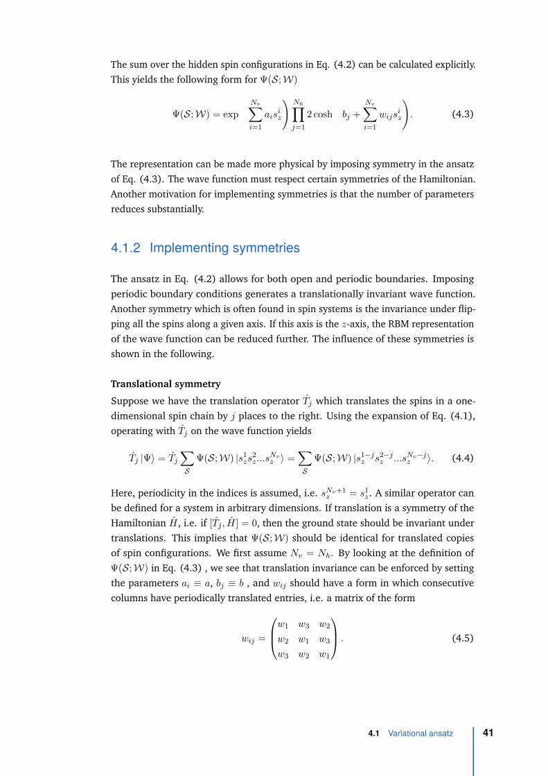
The sum over the hidden spin configurations in Eq. (4.2) can be calculated explicitly.This yields the following form for Ψ(S;W)

Ψ(S;W) = exp

(Nv∑

i=1

aisiz

)Nh∏

j=1

2 cosh

(bj +

Nv∑

i=1

wijsiz

). (4.3)

The representation can be made more physical by imposing symmetry in the ansatzof Eq. (4.3). The wave function must respect certain symmetries of the Hamiltonian.Another motivation for implementing symmetries is that the number of parametersreduces substantially.

4.1.2 Implementing symmetries

The ansatz in Eq. (4.2) allows for both open and periodic boundaries. Imposingperiodic boundary conditions generates a translationally invariant wave function.Another symmetry which is often found in spin systems is the invariance under flip-ping all the spins along a given axis. If this axis is the z-axis, the RBM representationof the wave function can be reduced further. The influence of these symmetries isshown in the following.

Translational symmetry

Suppose we have the translation operator Tj which translates the spins in a one-dimensional spin chain by j places to the right. Using the expansion of Eq. (4.1),operating with Tj on the wave function yields

Tj |Ψ〉 = Tj∑

SΨ(S;W) |s1

zs2z...s

Nvz 〉 =

∑

SΨ(S;W) |s1−j

z s2−jz ...sNv−j

z 〉. (4.4)

Here, periodicity in the indices is assumed, i.e. sNv+1z = s1

z. A similar operator canbe defined for a system in arbitrary dimensions. If translation is a symmetry of theHamiltonian H, i.e. if [Tj , H] = 0, then the ground state should be invariant undertranslations. This implies that Ψ(S;W) should be identical for translated copiesof spin configurations. We first assume Nv = Nh. By looking at the definition ofΨ(S;W) in Eq. (4.3) , we see that translation invariance can be enforced by settingthe parameters ai ≡ a, bj ≡ b , and wij should have a form in which consecutivecolumns have periodically translated entries, i.e. a matrix of the form

wij =

w1 w3 w2

w2 w1 w3

w3 w2 w1

. (4.5)

4.1 Variational ansatz 41

With these restrictions, the form of Ψ(S;W) becomes translationally invariant

Ψ(S;W) = exp

(Nv∑

i=1

aisiz

)Nh∏

j=1

2 cosh

(bj +

Nv∑

i=1

wijsiz

)

TI-symm.→ exp

(a

Nv∑

i=1

siz

)Nh∏

j=1

2 cosh

(b+

Nv∑

i=1

w1,(i+j−1)siz

),

(4.6)

where in the last line, we wrote the elements of the weight matrix wij of Eq. (4.5)explicitly in terms of the elements of the first column of the weight matrix

wij → w1,(i+j−1). (4.7)

Periodicity of the weights is implied by w1,(Nv+1) = w1,1. The parameter set isreduced from vectors with elements ai and bi to scalars a and b, and a matrix withelements wij to a vector with elements wi. The translation invariance can be seen inEq. (4.6). The exponential part is invariant under translation because the sum ofthe spins stays the same under translations. The product over the hidden nodes isalso invariant under translations, as translating the spins comes down to reshufflingthe order of the factors in the product.

The above considerations apply to the case Nv = Nh. One can introduce morehidden spins by an analogous construction. For example when Nh = 2Nv, theweight matrix of Eq. (4.5) now becomes rectangular and the periodic translation ofconsecutive columns is now implemented in square blocks

wij =

w11 w1

3 w12 w2

1 w23 w2

2

w12 w1

1 w13 w2

2 w21 w2

3

w13 w1

2 w11 w2

3 w22 w2

1

. (4.8)

In Eq. (4.8) the weight matrix consists of two square blocks which both consist ofperiodically translated columns in the same way as in the weight matrix of Eq. (4.5).The superscripts denote the index of the square blocks. There can now also be 2hidden biases. The hidden layer is thus in general split up in Nh/Nv filters whichall have the same structure as in the case of Nh = Nv but have of course differentvalues of the weights. The number of filters is denoted as

α ≡ Nv

Nh. (4.9)

We use the term filter because the operation on the spins in the arguments ofthe cosine hyperbolics of Eq. (4.6) resembles Eq. (2.5) defined in the context ofconvolutional neural networks. The weight vector in Eq. (4.6) is applied on theinput spin configuration and the cosine hyperbolic is taken of the resulting value.After that, the weight vector is moved one place to the left (or right) and the same


operation is done. This is repeated until we arive in the starting situation and all thecosine hyperbolics are multiplied. A minor downside of implementing translationalinvariance in this way is that the possible amount of hidden spins is a multiple of theamount of physical spins, whereas it is any natural number in the general case.

The translation invariant Ψ(S;W) for a general weight matrix can now be writtenas follows

Ψ(S,W) = exp

(a

Nv∑

i=1

siz

)Nv∏

j=1

α∏

f=1

2 cosh

(bf +

Nv∑

i=1

wi,(j+fNv)siz

). (4.10)

Spin flip symmetry

Another symmetry which can be implemented is spin flip invariance. The spin flipoperator for flips of all spins along the z-axis is defined as

Fz = σ1x ⊗ σ2

x ⊗ ...⊗ σNvx , (4.11)

as can be seen from Eqs. (1.7) and (1.8)

σx

∣∣∣∣sz = +1

2

⟩=

∣∣∣∣sz = −1

2

⟩and σx

∣∣∣∣sz = −1

2

⟩=

∣∣∣∣sz = +1

2

⟩. (4.12)

For [H, Fz] = 0, the wave function becomes invariant under spin flips , i.e. Ψ(S;W)

should be the same when all spins are flipped in the state. From Eq. (4.10), it isclear that both biases can be set to zero because they both introduce an asymmetrywith respect to spin flips. This yields the form

Ψ(S;W) =

Nv∏

j=1

α∏

f=1

2 cosh

(Nv∑

i=1

wi,(j+fNv)siz

). (4.13)

The above symmetries are straightforward to implement due to the structure of theRBM. Other symmetries may exist such as spin rotations

R(θ) = exp (−iθ · σ) , (4.14)

where σ is the vector of Pauli matrices defined in Eq. (1.8) and θ = θeθ is therotation vector defining a rotation around eθ by the angle θ. These symmetries cannot readily be implemented in the RBM.

Note that the implementation of symmetries reduces the parameters of the modeland enhances the computation time of the calculations. On the contrary, they canalso render the model not rich enough to learn efficiently. Not implementing these

4.1 Variational ansatz 43

symmetries can lead to more freedom in the ansatz which can help to guide thewave function to the set of parameters optimizing the state during the optimizationprocedure. However, the parameter set optimizing the state should respect thephysical symmetries which were explicitly implemented in this section. This issomething which should be kept in mind while doing simulations.

4.2 Optimizing the wave function

Eq. (4.3) provides a representation of the expansion coefficients of a wave function.From now on we focus on finding ground-state wave functions. Only for selectedvalues of the parameters ai, bi and wij , Eq. (4.3) approximates the ground statewell. The problem thus reduces to finding the set of parameters that approximatesthe ground state the best. What we mean by “best” will be introduced in thissection. The procedure of finding the optimal set of parameters is an iterative one.Thereby, we start with an initial state with random parameters and improve theapproximation step by step by updating all the parameters with small amounts untilsome convergence criterion is reached. How this is done is outlined in this section.

4.2.1 Initializing the wave function

The first step is to initialize the parameters in the ansatz of Eq. (4.3). In thecontext of neural networks, proper initialization of the parameters is crucial fordeep architectures [62]. Generally, initializing the parameters close to the expectedvalues is desirable, as it can make the optimization converge faster. It is naturalto assume that the initial weight distribution is centered around zero, because wedon’t know anything about the correlations in the system yet. The sign of a specificweight cannot be determined a priori. The variance of the distribution can be foundby inspecting Eq. (4.3). We see that it is the product of two kinds of functions:the exponential and the cosine hyperbolic. The exponential diverges fast for largepositive values of its input where a perturbation of the input makes a large differencein the output. On the other hand, it converges to zero for large negative values of itsinput, where a perturbation of the input makes negligible difference in the output.The cosine hyperbolic diverges for large negative and large positive values of itsinput and is insensitive to perturbations of the input around zero. It is natural toassume that the parameterset at the end of the optimization should be such that itresults in inputs of the exponential and cosine hyperbolic which are in their mostwell-behaved region. For the exponential, we can define this region as [−1, 1] wherethe output neither blows up or is approximately zero. For the cosine hyperbolic, thisregion lies around the values 1 and −1. From Eq. (4.3), we see that the parametersai and wij appear in a weighted sum of the input values. The sum of the spins (the


magnetization) is extensive in physical systems, i.e.∑Nv

i siz ∝ Nv. This means thatif we select the weights ai and wij to be approximately 1/Nv, the weighted sums∑Nv

i wijsiz and

∑Nvi ais

iz are proportional to 1, i.e. the input of the exponential and

cosine hyperbolic is well-behaved.

From the above considerations, it is natural to initialize the weights from a Gaussiandistribution with a mean of zero and standard deviation of 1/Nv, or from a uniformdistribution between −1/Nv and 1/Nv. The weights bj appear without weightingin the argument of the cosine hyperbolics of Eq. (4.3) and can thus be initializedfrom a Gaussian with a mean of zero and a standard deviation of 1 or a uniformdistribution between −1 and 1.

4.2.2 Update of the parameters

The next step is to update the parameters in the ansatz of Eq. (4.3) in an iterativeway, such that it approximates the ground state as well as possible. The main physicalingredient we use to accomplish this is the variational principle. The variationalprinciple states that a given state |Ψ〉 provides an upper bound on the exact ground-state energy of the system and converges to the ground state if it is tuned such thatthe energy functional

E[Ψ] =〈Ψ|H|Ψ〉〈Ψ|Ψ〉 (4.15)

is minimal [8]. Following the variational principle, we want to update the parametersin a way which decreases the energy of the wave function. This procedure iscalled variational Monte Carlo. The derivative of the energy gw with respect to anunspecified parameter w of the RBM (w ∈ {ai, bi, wij}) determines the change in theenergy induced by a variation of this parameter. Using the expansion of the wavefunction |Ψ〉 in the σz-basis (see Eq. (4.1)), we get

gw =∂

∂w

(〈Ψ|H|Ψ〉〈Ψ|Ψ〉

)=∑

S

[〈S|∂Ψ∗(S;W)

∂w H|Ψ〉+ 〈Ψ|∂Ψ(S;W)∂w H|S〉

〈Ψ|Ψ〉

]

−∑

S

〈Ψ|H|Ψ〉

(〈S|∂Ψ∗(S;W)

∂w |Ψ〉+ 〈Ψ|∂Ψ(S;W)∂w |S〉

)

〈Ψ|Ψ〉2

.

(4.16)

By defining Ow ≡ 1Ψ(S;W)

∂Ψ(S;W)∂w , Eq. (4.16) becomes

∂

∂w

(〈Ψ|H|Ψ〉〈Ψ|Ψ〉

)= 2 Re(〈HO∗w〉 − 〈H〉〈O∗w〉), (4.17)

4.2 Optimizing the wave function 45

where we used the shorthand notation 〈A〉 ≡ 〈Ψ|H|Ψ〉〈Ψ|Ψ〉 . The expectation values arewith respect to the wave function |Ψ〉. The expectation value of an operator A withrespect to the wave function |Ψ〉 can be written as

〈A〉 =〈Ψ|A|Ψ〉〈Ψ|Ψ〉 =

∑

S

Ψ(S;W)Ψ∗(S;W)

〈Ψ|Ψ〉〈S|A|Ψ〉Ψ(S;W)

, (4.18)

which can be computed using a Markov Chain Monte Carlo (MCMC) random walkin the configuration space of spin configurations S and treating |Ψ(S;W)|2

〈Ψ|Ψ〉 as the

probability distribution and the quantity A(S; Ψ) ≡ 〈S|A|Ψ〉Ψ(S;W) as the quantity that onemeasures. The random walk is constructed using the Metropolis-Hastings algorithm[63]. This algorithm consists of the following steps.

• Start with an initial state S0.

• Until a predefined number of steps Nsteps is reached, propose a new state S ′ byperforming an operation on the previous state Si−1 (e.g. by flipping a spin).

• Calculate the ratio r of the probability of S ′ and Si−1, i.e. r = |Ψ(S′;W)|2

|Ψ(Si−1;W)|2,

and define the acceptance ratio A as A = min (1, r).

• Draw a uniform random number u between 0 and 1. If u < r, accept the state,i.e. Si = S ′. If u ≤ r, reject the state, i.e. Si = Si−1.

In our case, the proposed updates are consecutive spin flips with respect to theprevious state Si−1. In this fashion, we run over the lattice NMC ≡ Nsteps/Nv times.One run over the lattice is called a sweep. We don’t calculate the quantity A(S; Ψ) atevery step in the Metropolis-Hastings algorithm, but rather once every sweep. Thereason is that the calculation of A(S; Ψ) is rather expensive and calculating it everystep brings little extra accuracy due to the autocorrelation time of A(S; Ψ). The meanof the set of values {A(S0; Ψ), A(SNv ; Ψ), ..., A(SNMCNv ; Ψ)} is an approximationof 〈A〉. In practice, the initial state S0 in the Metropolis-Hastings algorithm isdetermined by performing a thermalization run of the Metropolis-Hastings algorithmwith a random initial state and taking the final state of this thermalization run asthe initial state for the actual production run.

Having calculated the gradient gw, one can make use of gradient descent techniquesto update the parameters, so that it decreases the energy. The different techniquesthat we have adopted are described below. We denote with wt the value of anunspecified weight w at iteration step t and with gtw the gradient of Eq. (4.17) atiteration step t.


Gradient descent

The simple gradient descent consists of small updates of the parameters in thedirection of decreasing energy:

wt = wt−1 − lgt−1w . (4.19)

Here, l is the learning rate, a parameter which determines the rate of change ofthe parameter updates. This simple scheme suffers a number of very importantlimitations. The first limitation is the fact that the learning rate l is the same forevery parameter. If it happens that the gradients for some parameters are very small,and the gradients of other parameters are very large, one needs to adapt the learningrate to the large gradients because otherwise the method would become unstable.The cost function varies the most in the dimensions with large gradients, whichmeans that the updates in these dimensions should be small as to not overshootthe minimum. However, a small learning rate introduces very small updates ofthe parameters with small gradients which slows down convergence. The secondlimitation is the fact that this method might converge to a local minimum, ratherthan the global minimum. For general machine learning problems, this limitationis of less importance because a local minimum is often sufficient. Here, the realground state corresponds to the global minimum in parameter space. In general,one uses an annealing scheme, i.e. one lowers the learning rate during the iterationprocess to increasingly improve on the localization of the (local) minimum of thecost function.

Adagrad (adaptive gradient algorithm)

The adaptive gradient algorithm (Adagrad) extends gradient descent with a learningrate adapted to each parameter separately [64]:

wt = wt−1 − lt−1w gt−1

w , (4.20)

where lt−1w is calculated as follows:

lt−1w =

l√∑t−1t′=0 g

t′w

2+ ε

, (4.21)

where ε > 0 is a small number rather so as to avoid division by zero, and l is aparameter which tunes the overall magnitude of the different learning rates. Thismethod assigns a large learning rate ltw to the parameters corresponding with smallgradients and a small learning rate to parameters with large gradients. A nicebyproduct is that the learning rate diminishes upon further iteration (this can alsobe a disadvantage for some applications because the learning rate decays quitestrongly). The Adagrad method overcomes the problem of gradient descent that thegradients can be different in size, but not that the parameter updates stop when


a local minimum is reached. Another disadvantage is that the adaptations to thelearning rates take into account the gradients of all the iteration steps, while it maybe possible that the behaviour of the gradients changes during the iterations. Thisproblem is overcome in other, similar techniques, such as Adadelta (which takes intoaccount only a certain window of the previous gradients) [65].

Adam (adaptive moment estimation)

Adaptive moment estimation (Adam) uses the concept of momentum to avoidconverging to local minima [66]. Momentum means that the parameter updates useinformation from previous updates to construct the current update. On top of that,an Adagrad-like parameter-specific learning rate is used. The updates are describedas follows:

wt = wt−1 − l√vt−1w + ε

mt−1w . (4.22)

In this case, vtw and mtw are found as follows:

mtw =

β1

1− β1mt−1w + gtw,

vtw =β2

1− β2vt−1w + gtw

2.

(4.23)

Here, β1 and β2 are two parameters which govern the magnitude of influence ofthe previous gradients and l is a parameter governing the global magnitude ofthe updates. One can see from these equations that on a given step, the previousgradients influence the present update step, but with a weight exponentially decayingin iteration time. The learning rate is adapted in an Adagrad-like fashion, with anexponentially decaying influence of previous steps. This method is widely usedin machine learning. Although the method is a major improvement of the naivegradient descent, it can still be possible that the convergence fails. For example,pathological behaviour of the cost function can be detrimental to this method.The adaptation is gradual, meaning that the adaptation to sudden changes in thestructure of the cost function can take some iteration steps. For example, the updatesteps stay large when a sudden increase in the second derivative of the cost functionarises. Another problematic case are sharp bends in the structure of the cost function(see [67] for a visual representation of the concept of momentum).

Stochastic reconfiguration

We now turn to a method which is more suitable for variational Monte Carlo problems[68]. It is well known that the repeated application of the time-evolution operatorexp

(−iHt

)in imaginary time t→ −iτ ,

exp(−Hτ

), (4.24)


on a random quantum state |Ψ〉 (which is not orthogonal to the ground state) yieldsthe ground state of the system with Hamiltonian H. This can be seen by expandingthe random state |Ψ〉 in the eigenbasis of the Hamiltonian {|ψn〉} with energies {En}

|Ψ〉 =∑

n

cn |ψn〉 , (4.25)

where cn are the expansion coefficients. Applying operator (4.24) on the state |Ψ〉yields

exp(−Hτ) |Ψ〉 =∑

n

exp(−Enτ)cn |ψn〉 . (4.26)

We see that the eigenstates with higher energy are multiplied with exponentiallylower prefactors, and vanish approximately compared with the ground state when τbecomes large.

While this method works in theory, in practice one needs to resort to approximationmethods to this scheme. Indeed, there is no known technique to perform theoperation in Eq. (4.26) because the explicit operator is not known. One approach isto approximate the exponential operator of Eq. (4.24) for small τ to first order via aTaylor expansion

exp(−Hτ

)≈ 1− Hτ. (4.27)

Suppose we have a normalized quantum state |Φt〉 on a given iteration step t

|Φt〉 =|Ψt〉√〈Ψt|Ψt〉

, (4.28)

depending on the variational parameters {ai, bi, wij}. The derivatives of the nor-malized wave function to an arbitrary variational parameter w ∈ {ai, bi, wij} is

∂∣∣Φt⟩

∂w=

1√〈Ψt|Ψt〉

∣∣∣∣∂Ψt

∂w

⟩−

⟨Ψt∣∣∣ ∂Ψt

∂w

⟩

〈Ψt|Ψt〉|Ψt〉√〈Ψt|Ψt〉

. (4.29)

We can now write down the Taylor expansion of a quantum state for some perturba-tion δ around some parameterset w = {W}:

|Φt(w + δ)〉 = |Φt(w)〉+

Np∑

i=1

δi

∣∣∣∣∂Φt(w)

∂wi

⟩, (4.30)

where the number of parameters is denoted as Np. We now apply the first-orderexpansion in Eq. (4.27) of the imaginary-time evolution operator to the normalizedstate of Eq. (4.28). The result of this operation is written as a first-order Taylor


expansion of the quantum state as in Eq. (4.30). This yields the following equation

exp(−τH

)|Φt〉 ≈ |Φt〉 − τH |Φt〉 = |Φt+1〉 = |Φt〉+

Np∑

i=1

δi

∣∣∣∣∂Φt

∂wi

⟩, (4.31)

i.e. applying the imaginary-time evolution operator to the normalized state |Φt〉 isequivalent to updating the variational parameters w with the vector δ. By projectingEq. (4.31) on the derivatives of the wave function, we get

−τ⟨∂Φt

∂wj

∣∣∣∣ H∣∣∣∣Φt

⟩=

Np∑

i=1

δi

⟨∂Φt

∂wj

∣∣∣∣∂Φt

∂wi

⟩. (4.32)

By casting the indices to vectors, we can write this more concisely as

δ = −τS−1g, (4.33)

where δ is the vector of Taylor expansion coefficients δi, S is the matrix defined bythe elements

Sij =

⟨∂Φt

∂wi

∣∣∣∣∂Φt

∂wj

⟩, (4.34)

and g is the vector containing

gj =

⟨∂Φt

∂wj

∣∣∣∣ H∣∣∣∣Φt

⟩. (4.35)

One observes that the updates of the variational parameters are

wt+1 = wt + δ, (4.36)

where δ is found by calculating S and g and then inverting S.

The vector g is calculated by using the expression of Eq. (4.28) for the normalizedstate |Φt〉 in terms of the unnormalized state |Ψt〉 and the expression of Eq. (4.29)for the derivatives of the state |Φt〉 with respect to a parameter w:

gw =

⟨∂Φt

∂w

∣∣∣∣ H∣∣∣∣Φt

⟩=

1

〈Ψt|Ψt〉

⟨∂Ψt

∂w

∣∣∣∣ H∣∣∣∣Ψt

⟩−

⟨∂Ψt

∂w

∣∣∣Ψt⟩

〈Ψt|Ψt〉〈Ψt|H|Ψt〉〈Ψt|Ψt〉 . (4.37)

Calculating the derivatives of the wave functions in the σz-basis yields:

∣∣∣∣∂Ψt

∂w

⟩=∑

S

∂Ψt(S;W)

∂w|S〉 (4.38)

Inserting this in the expression for gw of Eq. (4.37), we get

gw = 〈O∗wH〉 − 〈O∗w〉〈H〉. (4.39)


The expression for the matrix S can be calculated in the same way

Sij = 〈∂Φt

∂wi|∂Φt

∂wj〉

=

⟨∂Ψt

∂wi

∣∣∣√〈Ψt|Ψt〉

−〈∂Ψt

∂wi|Ψt〉

〈Ψt|Ψt〉〈Ψt|√〈Ψt|Ψt〉

∣∣∣∂Ψt

∂wj

⟩

√〈Ψt|Ψt〉

−〈Ψt|∂Ψt

∂wj〉

〈Ψt|Ψt〉|Ψt〉√〈Ψt|Ψt〉

.

(4.40)

This equation reduces to the following form

Sij =〈∂Ψt

∂wi|∂Ψt

∂wj〉

〈Ψt|Ψt〉 −〈∂Ψt

∂wi|Ψt〉

〈Ψt|Ψt〉〈Ψt|∂Ψt

∂wj〉

〈Ψt|Ψt〉= 〈O∗wi

Owj 〉 − 〈O∗wi〉〈Owj 〉

(4.41)

The parameter updates can thus be calculated by evaluating the expectation values inEqs. (4.39) and (4.41), which can be done with an MCMC algorithm which samplesthe quadratic wave function, as described in the beginning of this section. Note theapparent difference in computational complexity between the methods which onlydepend on the gradients of the wave function (gradient descent, Adagrad and Adam)and the stochastic reconfiguration method. The methods depending on the gradientessentially scale asO(Np), where Np is the number of variational parameters. For thestochastic reconfiguration method, constructing the matrix S scales as O(N2

p ) andinverting it scales with O(N3

p ). This seems to render the stochastic reconfigurationmethod intractable because the cost of the updates increases rapidly with increasingnumber of parameters. The problem of inverting the matrix can be circumventedby using more advanced methods to invert matrices. In this work, we use theMINRES-QLP method to invert S [69]. We use the word inversion here for the realinverse or the pseudo-inverse, depending on whether the matrix is singular or not.The MINRES-QLP method is a method which solves the problem Ax = b by findingx such that x minimizes ‖Ax− b‖2, where ‖v‖2 denotes the 2-norm of the vector v,i.e.

‖v‖2 =

√√√√n∑

i=1

v2i , (4.42)

where n is the dimensionality of the vector v. The MINRES-QLP algorithm consistsof applying a Lanczos algorithm to the matrix A to cast it to a tridiagonal form.This algorithm applies the given matrix a number of times (typically lower thanthe number of rows/columns of the matrix) to a given testvector. This operationhas a computational complexity of O(k ×N2

p ), where k is the number of iterationsneeded to reduce A to a tridiagonal form. After the matrix A has been converted toa tridiagonal matrix, this matrix is used to minimize the norm ‖Ax− b‖2 in whatis called the MINRES-QLP phase of the algorithm. This phase not only minimizesthe norm, but als protects for numerical instabilities in the problem. The authors


of the MINRES-QLP algorithm claim that the complexity of this phase is betweenO(9Np) and O(14Np). The dominant cost of the whole algorithm is thus the tridiag-onalization of the given matrix: O(k ×N2

p ). We rewrite the matrix S of Eq. (4.41)as follows

Sij = 〈O∗wiOwj 〉 − 〈O∗wi

〉〈Owj 〉 = 〈(Owi − 〈Owi〉)∗(Owj − 〈Owj 〉

)〉

=1

NMC

∑

MCsamples

(Owi − 〈Owi〉)∗(Owj − 〈Owj 〉

)

=1

NMC

∑

MCsamples

[o∗oT

]ij,

(4.43)

where the vector o is a vector containing the list of Owi − 〈Owi〉 measured in theMCMC algorithm. By using this form of the matrix S, the multiplication of matrixand testvector in the Lanczos algorithm can be reduced to the multiplication of thevector o and the testvector of the Lanczos algorithm, and a multiplication of theresulting scalar with the vector o∗:

Sx =1

NMC

∑

MCsamples

o∗(o · x). (4.44)

This process scales as O(2Np), i.e. linear in the number of parameters.

By using these considerations, the complexity of the Stochastic reconfigurationscheme is reduced to a process ofO(Np), in line with the methods using the gradientsonly.

4.2.3 Convergence criteria

The updates of the parameters, as described in section 4.2.2, are stopped after asuitable number of iteration steps. We stop the updates of the parameters whenthe wave function converges to the ground state. For this, different criteria can beused. First, a stopping criterium based on the energy can be used. The expectationvalue of the energy is calculated in every iteration step to construct the estimatorof the gradient in Eq. (4.17). This energy can be compared to a reference energy,for example the exact energy of the ground state (if known) or the energy obtainedvia alternate techniques. When the relative energy error εE at an iteration stepdrops below a predefined tolerance value εtolE (e.g. εtolE < 10−3), the iterations can bestopped. A second stopping criterium is based on the moving average of the energy


not changing appreciably during some predefined number of iteration steps. A thirdcriterium is using the energy fluctuations, defined as

(∆E)2 = 〈H2〉 − 〈H〉2. (4.45)

For the ground state with energy Egs (and any other eigenstate of the Hamiltonian)Eq. (4.45) reduces to

(∆E)2 = E2gs − E2

gs = 0. (4.46)

When the energy fluctuations ∆E drop below a predefined tolerance value ∆Etol

(e.g. ∆Etol < 10−4), the iterations can be stopped. However, this stopping criterionis disfavoured compared to the other two because an additional expectation valueneeds to be calculated in every iteration, increasing the computing time.

4.2.4 Summary of the algorithm used to determine groundstates

initialize variational parameters (sec. 4.2.1)

sample current wave function for gradients

(sec. 4.2.2)

update variational parameters (sec. 4.2.2)

converged? (sec. 4.2.3)

terminate

yes

no

Fig. 4.2: Schematic depiction of the algorithm used to find the ground state of quantum spinsystems, as described in section 4.2.

We will now summarize the program flow of the algorithm used to find groundstates. This is also shown in figure 4.2.

1. Randomly initialize a state |Ψ〉 according to the ansatz of Eq. (4.3) whichhas the right symmetry for the Hamiltonian we try to find the ground statefor. This is done by initializing the weights to some small, non-zero value asdescribed in section 4.2.1.

2. Generate a set of NMC spin states {S} by sampling the probability distribution|Ψ(S;W)|2∑S |Ψ(S;W)|2 using an MCMC algorithm. This is described in section 4.2.2.


3. Use the generated samples of spin states to calculate the expectation values ofEq. (4.17) (and Eq. (4.41) if stochastic reconfiguration is used), and constructthe gradients.

4. Update the parameters of the RBM with a chosen scheme (for example gradientdescent, Adagrad, Adam or stochastic reconfiguration). This is outlined insection 4.2.2

5. Go to step 2 unless convergence is achieved. This is described in section 4.2.3.

4.3 Theoretical properties and other methods

4.3.1 Theoretical properties

We now investigate the RBM approach for modelling quantum many-body systemsfrom a theoretical point of view by examining the available literature. We first treatthe entanglement entropy of many-body wave functions represented by RBMs. Theentanglement entropy Se is defined as

Se(ρA) = −Tr(ρA log(ρA)) = −Tr(ρB log(ρB)), (4.47)

where A is a subsystem of the system and B is its complement. Furthermore, ρA isthe density matrix associated with the subsystem A, defined as

ρA = TrB(ρ), (4.48)

where ρ is the density matrix of the system (see Eq. (1.17)) and TrB is a traceover the degrees of freedom associated with the subsystem B. The entanglemententropy is a measure for the (quantum) correlations between subsystems A andB [70]. It can be associated with the information gain: when measuring the stateof subsystem A, the entanglement entropy determines how much information canbe gained about the subsystem B. For quantum states arising from local gappedHamiltonians (i.e. Hamiltonians for which the ground and first excited states have adifference in energy) it is believed that the entanglement entropy of a subsystem A

of size Ld scales (in leading order) as

Se(ρA) = cLd−1, (4.49)

where d is the dimension of the system. This has been proven for 1D systems[71], but remains an open question for systems of more than one dimension. Theentanglement entropy is thus proportional to the surface of the subsystem and not to


the volume of the subsystem, as would be expected from the extensivity of (classical)entropy. This is the so-called area-law of entanglement. Because entanglemententropy is a measure for correlations, it follows that the correlations between A andB are present at the surface of the subsystem, i.e. they are short-range.

The entanglement entropy for RBM states was investigated in [72]. They provedthat the wave function as described in section 4.1 obeys a volume-law entanglement,i.e. it is capable of modelling quantum states with entanglement entropy scalingas Se(ρA) = cLd. When the RBM is restricted to short range correlations (i.e. theweights originating from a hidden node are only non-zero for a finite range ofvisible spins (cfr. convolutional neural networks)), the states follow an area-lawentanglement.

The RBM wave function has also been used to represent quantum states exactly. Thefirst example is the 1D symmetry protected cluster state [73], i.e. the ground stateof the following Hamiltonian

Hcluster = −Nv∑

i

σi−1z σixσ

i+1z , (4.50)

where periodic boundary conditions are implied. The second example are the groundstates of the 2D Kiteav Toric code [74] with Hamiltonian

HKTC = −∑

+

∏

i∈+

σiz −∑

�

∏

i∈�σix. (4.51)

Here, the spins are placed on the edges of a square lattice. The symbol + denotesthe four spins neighbouring a vertex of the lattice, i.e. the sum

∑+ runs over all

lattice points. The symbol � denotes a square of the square lattice, i.e. four edges ina square. The sum

∑� runs over all squares of the lattice. Also for this Hamiltonian

periodic boundary conditions are implied. Determining the wave functions exactlywith an RBM entails finding the weights and biases {ai, bi, wij} such that Eq. (4.1),with Ψ(S;W) determined by Eq. (4.2), represents the state exactly.

4.3.2 Other methods

Apart from the (very) limited amount of exactly solved quantum many-body prob-lems (such as the transverse field Ising model in section 4.4.1), there exists a wealthof approximation methods of which we briefly mention a selection of important oneshere. Most of the methods have the aim to compress the quantum states in a formal-ism which is exponentially cheaper than the general formalism described in section1.2, i.e. one wants to go from a formalism with O(exp(N)) free parameters to a

4.3 Theoretical properties and other methods 55

formalism with a number of free parameters which scales for example polynomiallywith system size.

The method which is closest to the original formulation of the problem (i.e. di-agonalizing the Hamiltonian matrix) is the exact diagonalization technique. Theexact diagonalization method for finding ground states of quantum systems entails adiagonalization of the Hamiltonian matrix in a subspace of the full Hilbert space.One of the possible methods to find this subspace is the Lanczos algorithm [75]:

1. Start with a random normalized state |Ψ0〉, which is not orthogonal to theground state.

2. If we would apply one step of the gradient descent algorithm (described insection 4.2), the new state will lie in the space spanned by |Ψ0〉 and |Ψ1

g〉,where |Ψ1

g〉 is the normalized state which is proportional to the functionalderivative of the energy functional to the current state |Ψ0〉

|Ψ1g〉 =

δ 〈Ψ|H|Ψ〉δ |Ψ〉

∣∣∣∣∣|Ψ0〉

. (4.52)

3. If we would apply the gradient descent algorithm n times, the resulting statewill lie in the space spanned by {|Ψ0〉 , |Ψ1

g〉 , |Ψ2g〉 , ..., |Ψn

g 〉}, which is oftencalled the Krylov space. An orthonormal basis for this subspace can be con-structed via an iterative algorithm. In this basis, the Hamilonian matrix istridiagonal, which can be efficiently diagonalized (in O(n log(n)) computa-tional time [76]). The eigenstate with the lowest eigenvalue is then found tobe an approximation of the ground state.

This approach thus avoids the curse of dimensionality of the matrix diagonalization.However, the problem with this approach is that the different states need to bestored exactly, which requires an exponential amount (as a function of system size)of expansion coefficiens (see section 1.2). This method is thus only feasible for smallsystems.

Another successful method to find ground states of many-body system is the densitymatrix renormalization group (DMRG) [77]. This method provides the ground stateof a system of N degrees of freedom by iteratively constructing it. The construc-tion follows the following steps (we employ the example of a spin system as anillustration) [78]:


1. Start with two spins and find the eigenspectrum of the system using diagonal-ization of the Hamiltonian matrix.

2. Until the desired system size N is reached, suppose we have at some step 2l

degrees of freedom. These are divided in two blocks A and B of size l. Twonew degrees of freedom are added to the system by placing them between Aand B. The resulting (arbitrary) state can then be written as

|Ψ2l+2〉 =∑

θA,θB ,λA,λB

Ψ(θA, θB, λA, λB) |θA〉 |θB〉 |λA〉 |λB〉 , (4.53)

where |θA〉 (|θB〉) is the basis state associated with block A (B) and |λA〉 (|λB〉)is the basis state associated with the new degree of freedom next to block A(B).

3. The eigenspectrum of the new system is found and a new basis is constructedfor the new blocks A+ (B+) (formed by appending the new spin next to A (B)to the block A (B)). This new basis for A+ (B+) is defined by constructingthe density matrix ρΨ2l+2

gsof the ground state and taking the reduced density

matrix ρA+ (ρB+) of block A+ (B+) defined as

ρA+ = TrB+(ρΨ2l+2gs

), (4.54)

after which one diagonlizes ρA+ (ρB+) and keeps only the D eigenstatescorresponding to the D highest eigenvalues. In this way, the number of basisstates of the blocks does not grow during the iterations, but stays constant. Thisreduces the cost of representing a state compared to keeping all the basis states,in which case the number of basis states of the blocks grows exponentiallywith block size.

The DMRG procedure naturally results in the concept of tensor networks (TN). Itcan be proven that the states resulting from a DMRG algorithm are states whichfall in the class of matrix product states (MPS) [79]. MPS are states which canbe written as a product of matrices, i.e. every degree of freedom corresponds to aunique matrix. The matrices are contracted with each other to yield the expansioncoefficients of a quantum state. This can be written down as

|Ψ〉 =∑

{λi}

Tr(A(λ1)A(λ2)...A(λN )) |λ1λ2...λN 〉 , (4.55)

where λi are the different basis states associated with the i-th degree of freedom(e.g. the σz-basis states of Eq. (1.11)) and A(λi) is a matrix associated with basisstate λi. The trace reflects the periodic boundary conditions. Loosely speaking, the

4.3 Theoretical properties and other methods 57

contraction of the matrices represents the interaction between two neighbouringdegrees of freedom. The matrices A have a small dimension compared to the totalnumber of basis states. This dimension is called the bond dimension and determineshow many parameters are available to describe the quantum states. The bonddimension is intimately related to the entanglement entropy Se of Eq. (4.47) of thestate. The bond dimension provides a bound on the maximal entanglement entropyof an MPS [80]. The MPS can be generalised to a general tensor network, wheretensors with an arbitrary number of indices are contracted in a specific way. Thismakes it possible to for example define tensor networks for systems in more thanone dimension. It can be proven that tensor networks fall in the class of modelswhich can describe states with area-law entanglement [80]. Finding the parametersof tensor networks can be done for example by using the variational monte carloapproach, as described in section 4.2 [81] or by a DMRG-like algorithm, where oneiteratively optimizes every tensor via a diagonalization procedure [82].

Fig. 4.3: Schematic depiction of the ansätze described in Ref. [61]. The shaded areas depicthow the different degrees of freedom on a 2D lattice functionally depend on eachother in the ansatz. The different ansätze are (a) the Jastrow ansatz, (b) matrixproduct states, (c) entangled plaquette states and (d) string bond states. Figureadapted from [61].

The RBM states presented in this chapter can be related to other variational ansätzefor many-body quantum states. It has been proven that the RBM states can be relatedto tensor network states [74]. Spefically, Ref. [74] provided constructive algorithmsto write MPSs as RBMs and vice versa. Because RBMs can represent states withvolume-law entanglement (see section 4.3.1), which is only possible for MPSs whenthe bond dimension grows exponentially with system size, the RBMs can representthese states with an exponentially lower amount of resources. However, this doesnot mean that RBMs are better as a variational ansatz: volume-law entanglementis by far not always required (see section 4.3.1) and the success not only dependson the representational power but also on the algorithms to actually find the states.Another related class of states [61] is the Jastrow ansatz, which can be written as

|Ψ〉Jastrow =∑

S

∏

siz<sjz

fi,j(siz, s

jz) |s1

zs2z...s

Nvz 〉 , (4.56)


where fi,j(siz, sjz) is a function representing two-body interactions between spin i

and spin j. The RBM can represent any Jastrow function with Nh = (Nv − 1)Nv/2

hidden units. Ref. [61] also showed that RBMs can be written as string-bond states(SBS), which are a product of different MPSs snaking over a 2D lattice:

|Ψ〉SBS =∑

S

∏

j

Tr(∏

i∈jAi,j(s

iz)) |s1

zs2z...s

Nvz 〉 , (4.57)

where j is the index identifying the different snakes over the lattice and i is the indexidentifying the lattice vertices the snakes run over. Finally, Ref. [61] showed thatshort-range RBMs can be written as entangled plaquette states (EPS), defined as

|Ψ〉EPS =∑

S

M∏

i=0

Pi(S) |s1zs

2z...s

Nvz 〉 , (4.58)

where i identifies local subsets of spins (plaquettes) and Pi(S) is a function of thespins in these subsets. The different ansätze are schematically depicted in figure4.3.

4.4 Quantum spin systems

While the RBM approach outlined in sections 4.1 and 4.2 works for any finite (dis-crete) quantum system, we will use the method to find ground states and propertiesof quantum spin systems. These spin systems describe models for magnetism. Whilethis is interesting in itself, the most interesting feature of quantum spin systems isthat they serve as an excellent prototypical quantum system, exhibiting featuresalso found in other systems. These features include phase transitions, superposition,entanglement, frustration effects, etc. The fact that these models are discrete innature make them attractive from a computational point of view.

4.4.1 Transverse field Ising model

The transverse field Ising model (TFI) is defined by the Hamiltonian of Eq. (1.14).The TFI model has an exact solution in one dimension. This was given by Pfeutyin 1970 [83] by using the Jordan-Wigner transformation and solving the resultingeigenvalue problem. The result is a ground-state energy with magnitude

Egs = −j∑

k

Λk, (4.59)

where Λk is given by

Λk =

√1 + 2g cos(k) + (g)2. (4.60)

4.4 Quantum spin systems 59

The variable k runs over the discrete set of possible wavevectors in the first brillouinzone, i.e. k ∈ [−π, π], where k can have values (for even Nv, which we will alwayschoose)

k = −π(Nv − 1)/Nv,−π(Nv − 3)/Nv, ..., π(Nv − 3)/Nv, π(Nv − 1)/Nv. (4.61)

This exact solution is extremely useful with the eye on benchmarking numericalcalculations.

As stated in the introduction, the TFI model undergoes a phase transition betweena disordered state (with zero absolute magnetization 〈|sz|〉) and an ordered state(with non-zero absolute magnetization 〈|sz|〉). Absolute magnetization is defined as

〈|sz|〉 =

⟨∣∣∣∑Nv

i=1 σiz

∣∣∣⟩

Nv, (4.62)

which is the quantum counterpart of the classical magnetization of spin systemsdefined in Eq. (2.3).1 In one dimension the phase transition occurs at j = h = 1,or gc = 1. In two-dimensions, the TFI model undergoes a phase transition atj = 1, h = 3.05266..., or gc = 3.05266.... For h � j, the system is in a disorderedstate, whereas for j � h an ordered state with non-vanishing magnetization isfound. One can prove that the phase transition is second order [84]. This meansthat the response function of the thermodynamic variables, e.g. the specific heator the susceptibility, diverge at the critical point. The 1D TFI belongs to the sameuniversality class as the 2D classical Ising model described in section 1.1 [85]. Auniversality class is defined as a collection of models which share the same large-scale behaviour at a second order critical point [3]. One of the consequences is thatthey share the same critical exponents.

The TFI model has a spin flip symmetry (Z2-symmetry) meaning that the Hamiltonianis invariant under the operator F , defined in Eq. (4.11). In the magnetically orderedphase (h < 1 for one-dimensional systems), this symmetry is broken and there existtwo degenerate ground states with opposite total spin.

With the eye on the discussion of chapter 5, we mention the characteristics of the firstexcited states of the 1D TFI model [84]. For ordered states, the first excited statescorrespond to states with two domain walls2, i.e. a collection of neighbouring spinswith arbitrary size 0 < l < Nv is flipped with respect to the ground state. States withdomain walls of size l and of sizeNv−l have opposite magnetization. This means thata linear combination of these two kinds of states (with equal weights) has vanishing

1We use the absolute magnetization because the ground state in the ordered phase is doubly degener-ate with opposite magnetizations.

2There are two domain walls due to the periodic boundary conditions. With open boundary conditions,the first excited state would correspond to states with one domain wall.


magnetization. Because the states represented by RBMs imply spin flip symmetry,these states indeed have equal weight, resulting in a vanishing magnetization whenmeasured. For disordered states, the first excited state is obtained by flipping a spinin the ground state.

The TFI model is often used as a benchmark for new algorithms that are designed tosolve the quantum many-body problem. Indeed, the TFI model is one of the simplestmodels for spins on a lattice, while non-trivial in terms of its interactions.

4.4.2 Antiferromagnetic Heisenberg model

The antiferromagnetic Heisenberg model (AFH) is defined by the Hamiltonian

HAFH =∑

〈i,j〉

σixσjx + σiyσ

jy + σizσ

jz, (4.63)

where∑〈i,j〉 denotes a sum over all pairs of nearest neighbours and σix, σiy, σ

iz are

the Pauli matrices defined in Eq. (1.8), acting on the spin with index i.

The AFH model is invariant under the total spin operator,

S =∑

i=1

Nv

sixsiysiz

. (4.64)

Indeed, the Hamiltonian commutes with S,

[HAFH , S] = 0. (4.65)

This can be seen by using the commutation and anticommutation relations of thePauli matrices of Eqs. (1.9) and (1.10). The AFH model is also invariant under spinrotations (i.e. SU(2) invariance)

[HAFH , R(θ)] = 0. (4.66)

The spin rotation operator R(θ) is defined in Eq. (4.14). To prove Eq. (4.66), theexponential in the spin rotation operator can be expanded in a Taylor series andrewritten in terms of its real and complex parts, yielding

R(θ) = cos(θ)I − iσ · eθ sin(θ). (4.67)

4.4 Quantum spin systems 61

The first term commutes with the Hamiltonian because it is proportional to the unitoperator. The second term commutes because it is proportional to the total spinoperator, which commutes with the Hamiltonian (see Eq. (4.65)).

The one-dimensional AFH model has a disordered ground state. This propertyfollows directly from the Mermin-Wagner theorem, which states that a continuoussymmetry of the system (in this case the SU(2)-symmetry) cannot be broken inclassical systems of dimension d < 3 [86]. For quantum systems, we can makeuse of the relation between d-dimensional quantum systems in the ground stateand (d+ 1)-dimensional classical systems at finite temperature (see section 1.4) tofind that a continuous symmetry cannot be broken in a system of dimension d < 2.The SU(2)-symmetry of the AFH model can thus be broken in the two-dimensionalsystem. This is the case for the AFH model, which exhibits a non-zero staggeredmagnetization (Néel order) in two dimensions [87].

Both the one and two dimensional AFH models exhibit long-range correlations intheir ground state, decaying polynomially with distance [87, 88].

4.5 Results

4.5.1 Ground-state energy

Tab. 4.1: Learning rates l used for figures 4.4, 4.5, 4.6 and 4.7 (see section 4.2.2 for theirdefinition). These learning rates are the ones which lead to the lowest energy.

1D TFI 1D AFH 2D TFI 2D AFHgradient descent 0.0005 0.0005 0.0005 5× 10−5

Adam 0.007 0.003 0.005 0.0005

Adagrad 0.05 0.05 0.04 0.005

stochastic reconfiguration 0.4 1.0 0.1 0.2

We will start with the situation Nh = Nv and reproduce the results of [57]. Wefirst compare the different minimization methods on small systems. For all thedifferent runs, we used 1000 Monte Carlo samples (from 1000 sweeps over thelattice, see section 4.2.2) per iteration step to estimate the expectation values of Eqs.(4.41) and (4.17). This number is a balance between accuracy and computationtime per iteration step: when the number of MC samples is increased, the accuracyof the gradients increases, but this also increases the computation time per step.It is well-known in machine learning that noisy estimators of gradients performcomparably well in finding the minimum of a cost function compared with moreaccurate estimates [89]. However, noisy estimators come with an increase in the


number of iteration steps needed for convergence. This technique is called StochasticGradient Descent (SGD). The learning rates l are summarized in table 4.1. Theselearning rates yield the lowest energy compared to other learning rates. When theAdam method in Eq. (4.22) is used, we take β1 = 0.9, β2 = 0.99 in Eq. (4.23).

0 200 400 600 800 1000

iteration number

0.00

0.05

0.10

0.15

0.20

0.25re

lati

veen

ergy

erro

rε E

=∣ ∣ ∣E−Egs

Egs

∣ ∣ ∣ 1D TFINv = 40

h/j = 1

α = 1

gradient descentAdamAdagradstochastic reconfiguration

600 700 800 900 1000

10−4

10−3

10−2

10−1

Fig. 4.4: Convergence of the energy of the 1D TFI system (j/h = 1, Nv = 40 and α = 1) asa function of the number of iteration steps for different learning algorithms. Theenergy error is with respect to the exact ground-state energy Egs of Eq. (4.59)(Egs/Nv = −1.2736j). The inset shows the last 400 steps on a logarithmic scale inorder to illustrate the magnitude of the fluctuations of the energy once convergenceis reached.

Figure 4.4 shows the convergence of the energy for the one-dimensional TFI modelat g = h/j = 1 relative to the exact result described in section 4.4.1 (see Eq.(4.59)). We see that all the different learning algorithms perform well in terms ofenergy convergence. Differences can be seen in the convergence speed3, where thestochastic reconfiguration scheme converges the fastest and the gradient descentmethod the slowest. Although faster, the stochastic reconfiguration does not appearto be the optimal method in terms of attaining the lowest energy value. In this case,the Adam method is capable of attaining the lowest energy values. Note, however,that the stochastic reconfiguration method reaches its lowest energy value afterapproximately 100 iteration steps, after which the energy increases slightly and startsto converge again but more slowly. This can point in the direction that a betterfine-tuning of the learning rate would result in a more monotonous decrease ofthe energy. All learning schemes perform well, and result in an accuracy at thesubpercent level after 1000 iterations.

3We use the term speed to denote how fast some quantity converges in terms of iteration steps.The term computation time denotes the time it takes in seconds for a certain computation to beperformed.

4.5 Results 63

0 200 400 600 800 1000

iteration number

0.00

0.05

0.10

0.15

0.20

0.25

0.30

0.35

0.40

0.45

rela

tive

ener

gyer

rorε E

=∣ ∣ ∣E−Egs

Egs

∣ ∣ ∣ 1D AFHNv = 40

α = 1


600 700 800 900 1000

10−5

10−4

10−3

10−2

10−1

Fig. 4.5: Convergence of the energy of the 1D AFH system (Nv = 40 and α = 1) as a functionof the number of iteration steps for different learning algorithms. The energy erroris with respect to the ground-state energy Egs obtained with quantum Monte Carlosimulations using the ALPS software [90] (Egs/Nv = −1.7746). The inset showsthe last 400 steps on a logarithmic scale in order to illustrate the magnitude of thefluctuations of the energy once convergence is reached.

Figure 4.5 shows the energy convergence of the 1D AFH model. The energy isrelative to the energy of quantum Monte Carlo simulations of the AFH at finitetemperature extrapolated to zero temperature [90]. In figure 4.5, the power of thestochastic reconfiguration method is more clear than in the one-dimensional TFIcase. Here, we see that the speed of convergence is much faster than all the othermethods, especially than the gradient descent method. Stochastic reconfigurationalso reaches the lowest energy compared to the other methods.

Figure 4.6 shows the energy convergence of the 2D TFI model at j/h = g = 3.05266

relative to the energy obtained via exact diagnonalization [91]. We see that alloptimization methods converge fast and approximate Egs well. The final energy ofthe stochastic reconfiguration method is again the lowest, in this case comparablewith the Adam method.

Figure 4.7 shows the energy convergence for the 2D AFH model relative to quantumMonte Carlo simulations [92]. This figure provides the most compelling informationon the performance of the learning methods. Here, we see that only the stochasticreconfiguration method reaches acceptable energy values, whereas the Adagrad andgradient descent methods are barely able to reach 10 percent of the true ground-stateenergy in an acceptable amount of iteration steps. For the Adam method, matters


0 200 400 600 800 1000

iteration number

0.00

0.02

0.04

0.06

0.08

0.10

0.12

rela

tive

ener

gyer

rorε E

=∣ ∣ ∣E−Egs

Egs

∣ ∣ ∣ 2D TFINv = 36

h/j = 3.05266

α = 1


600 700 800 900 1000

10−6

10−5

10−4

10−3

10−2

Fig. 4.6: Convergence of the energy of the 2D TFI system (j/h = 0.32758, Nv = 36 and α =1) as a function of the number of iteration steps for different learning algorithms.The energy error is with respect to the ground-state energy Egs obtained via exactdiagonalization results [91] (Egs/Nv = −3.2473j). The inset shows the last 400steps on a logarithmic scale in order to illustrate the magnitude of the fluctuationsof the energy once convergence is reached.

are even worse because the energy diverges and settles at an error of 30 percent.This behaviour is most likely due to large variations in the Hessian matrix C of theenergy surface, definded as

C =

∂2E∂w1∂w1

. . . ∂2E∂w1∂wNp

.... . .

∂2E∂wNp∂w1

∂2E∂wNp∂wNp

, (4.68)

where Np is the number of parameters in the model. This is the matrix describingthe curvature of the energy surface. Large values in the Hessian may cause divergentbehaviour for methods where momentum is involved (for a nice interactive accountof these effects, see [67]).

In conclusion, using an RBM representation of the ground-state wave function, theenergy converges to within 1% of the known value after 1000 iterations or lessfor all the considered models, even with a low amount of variational parameters.The stochastic reconfiguration technique performs systematically better in terms ofconvergence speed. With the stochastic reconfiguration method, initial fluctuationsare present, after which the energy drops fast. The other minimization techniquesrequire a larger amount of iteration steps to converge to a low energy value. Also in

4.5 Results 65

0 200 400 600 800 1000

iteration number

0.0

0.1

0.2

0.3

0.4

0.5

0.6

0.7

0.8

rela

tive

ener

gyer

rorε E

=∣ ∣ ∣E−Egs

Egs

∣ ∣ ∣ 2D AFHNv = 100

α = 1


600 700 800 900 1000

10−3

10−2

10−1

100

Fig. 4.7: Convergence of the energy of the 2D AFH system (Nv = 100 and α = 1) as afunction of the number of iteration steps for different learning algorithms. Theenergy error is with respect to the ground-state energy Egs obtained with quantumMonte Carlo simulations of [92] (Egs = −2.6862). The inset shows the last 400steps on a logarithmic scale in order to illustrate the magnitude of the fluctuationsof the energy once convergence is reached.

terms of energy minimization, the stochastic reconfiguration technique converges tothe lowest energy for all but the 1D TFI system. From these considerations, it is clearthat the stochastic reconfiguration method is the most favorable for wave functionoptimization. This comes with the cost of slightly increased computation times due tothe matrix inversion in the method, as shown in Eq. (4.33). In the remainder of thiswork, the stochastic reconfiguration method will be used to perform minimization ofvariational wave functions, unless stated otherwise.

4.5.2 Scaling

We now investigate how the procedure to find variational wave functions with RBMsscales with the system size Nv and with the number of variational parameters Nh.For this, we investigate the 1D TFI model at g = h/j = 1. Figure 4.8 displays thescaling of the proposed algorithm with system size. We simulate system sizes from10 to 100 spins. We choose α = 4 (see Eq. (4.9)) as a compromise between accuracyand computation time per step. The CPU-times are measured and a power law isfitted to these data points. The CPU time scales approximately quadratically withsystem size: tCPU = 0.00673N1.929

v − 0.217. This can be attributed to the fact thatthe size of the weight matrix of Eq. (4.8) scales quadratically with system size.This matrix is used in the evaluation of the expectation values of Eqs. (4.17) and


0 20 40 60 80 100

number of spins Nv

−10

0

10

20

30

40

50

60

CPU

tim

epe

rit

erat

ion

step

t CPU

[s]

fit to CPU timesCPU time

0 20 40 60 80 100

number of spins Nv

0

1

2

3

4

5

6

rela

tive

ener

gyer

rorε E

=∣ ∣ ∣E−Egs

Egs

∣ ∣ ∣

×10−4

1D TFI, α = 4, g = gc = 1

Fig. 4.8: Scaling as a function of system size for the 1D TFI model. Left: scaling of CPUtime tCPU per iteration step as a function of system size. The green line is a powerlaw (tCPU = 0.00673N1.929

v − 0.217) fit to the CPU-times. Right: scaling of energyconvergence εE (with standard error) with system size.

(4.41) required to perform the optimization steps. From figure 4.8, we also seethat the energy error becomes smaller with increasing system size. This can beappreciated by noting that larger system sizes induce more variational parameters(Nh = αNv). The variational parameters need to describe the correlations betweenthe spins. These correlations decay with distance. Effectively, this means that thenumber of parameters grows faster than the correlation in the system, facilitatingthe description of these correlations for larger systems.

The scaling with the number of variational parameters is depicted in figure 4.9.We simulated the TFI model with Nv = 40 for values of α between 1 and 16.We see that the CPU-times per step scale polynomially with system size (tCPU =

1.147α1.283 + 0.908). The scaling is close to linear in the number of parameters. Thisis to be expected from the MINRES-QLP matrix inversion, which scales linearly inthe number of variational parameters (see Eq. (4.43) and its discussion). The energyerror decreases monotonously with increasing number of variational parameters.This is expected from the variational principle, but is still reassuring as the methodis non-linear in the variational parameters and its success does not only depend ontheoretical bounds, but also on the optimization algorithm. The optimization of thevariational parameters can fail, even when it is theoretically feasible. This propertyis well-known in the machine learning community and especially arises in the fieldof deep learning [62]. Because RBMs are shallow networks, this problem can still bepresent but should be under control.

4.5 Results 67

0 2 4 6 8 10 12 14 16 18

hidden to visible ratio α

0

5

10

15

20

25

30

35

40

45C

PUti

me

per

step

t CPU

[s]

fit to CPU timesCPU time

0 2 4 6 8 10 12 14 16


10−5

10−4

10−3

10−2

rela

tive

ener

gyer

rorε E

=∣ ∣ ∣E−Egs

Egs

∣ ∣ ∣

1D TFI, Nv = 40, g = gc = 1

Fig. 4.9: Scaling as a function of the ratio of the number of hidden variables to the numberof visible variables α. Left: scaling of CPU time tCPU per iteration step as afunction of the number of parameters. The green line is a power law (tCPU =1.147α1.283 + 0.908) fit to the measured CPU times. Right: scaling of energyconvergence εE (with standard error) with the number of parameters.

4.5.3 Energy fluctuations

In section 4.2.3, we showed that the relative energy fluctuations ∆E/E defined inEq. (4.45) provide a good way to verify if the variational wave function convergedto the ground state. A proper representation of the ground state should have a lowvalue for ∆E/E (see Eq. (4.46)). The relative energy fluctuations are depicted infigure 4.10. We see a systematic improvement to lower values of the relative energyfluctuations when increasing the number of variational parameters.

4.5.4 Comparison with literature

We compare the relative energy error on the ground state for the 2D TFI and AFHmodels with results in the available literature. We optimize the 2D TFI ground stateon a square lattice with size 6× 6 at the critical point (gc = 3.05265897...) and the2D AFH model on a square lattice with size 10 × 10. The energy convergence ismeasured for different values of α (see Eq. (4.9)), relative to the values of [91] (TFI)and [92] (AFH), which we also used in section 4.5.1. The results are shown in figure4.11. For the TFI model, we compare with correlator product states (CPS) [93]and tree tensor networks (TTN, see tensor networks in section 4.3.2) [94]. We seethat the relative energy error is lower than that obtained with CPS and approaches


0 2 4 6 8 10 12 14 16


10−6

10−5

10−4

rela

tive

ener

gyflu

ctua

tion

s∆E E

1D TFINv = 40, g = 1

0 2 4 6 8 10 12 14 16


10−6

10−5

10−4

rela

tive

ener

gyflu

ctua

tion

s∆E E

1D AFH, Nv = 40

Fig. 4.10: Relative energy fluctuations ∆E/E as a function of the ratio of the number ofhidden variables to the number of visible variables α for the 1D TFI and the 1DAFH models. This measure is important to determine the quality of the resultingground state, where the energy fluctuations should vanish.

the value quoted for TTN. It is interesting to note that the CPS and TTN ansätzehave 65536 and O(108) parameters respectively, whereas for α = 16 we have 20736

parameters in the weight matrix of Eq. (4.8), of which 576 are unique. For the AFHmodel, we compare with entangled plaquette states (EPS, see section 4.3.2) [95] andprojected entangled pair states (PEPS, see tensor networks in section 4.3.2) [96]. Wesee that our RBM ansatz does not achieve the accuracy of these two methods. Therelative energy error drops with increasing α, but rises again4 for α = 16. However,Refs. [57, 58] reported lower relative energy errors with the same RBM ansatz. It isunclear why this discrepancy between this work and other RBM implementationsis present, but one possibility is that the hyperparameters (i.e. the learning rate,the learning rate annealing, the number of MC samples, ...) are better tuned in theworks of [57, 58] compared to our work.

4This may be due to too little runs. For α = 16 we only did 3 different runs because of the highercomputational cost. We did of the order of 20 runs for the other values of α.

4.5 Results 69

5 10 15 20


10−8

10−7

10−6

10−5

10−4re

lati

veen

ergy

erro

rε E

=∣ ∣ ∣E−Egs

Egs

∣ ∣ ∣

CPS

TTN

6× 6 2D TFIg = 3.05265897

5 10 15 20


10−3

10−2

rela

tive

ener

gyer

rorε E

=∣ ∣ ∣E−Egs

Egs

∣ ∣ ∣

EPS

PEPS

10× 10 2D AFH

Fig. 4.11: Comparison of relative energy errors on the ground states of the 6× 6 critical 2DTFI model and the 10 × 10 2D AFH model with other variational ansätze. Theenergies are relative to the energy obtained with exact diagonalization [91] forthe TFI and with quantum Monte Carlo [92] for the AFH. We compare our resultswith correlator product states (CPS) and tree tensor networks (TTN) for the TFIand with entangled plaquette states (EPS) and projected entangled pair states(PEPS) for the AFH.

4.5.5 RBM representation as a function of iteration step

An interesting aspect of the RBM representation of quantum states is how exactlythey represent the quantum states. This information is encoded in the weight vectorsof Eq. (4.10). The weight vectors encode the correlations present in the wavefunction. This is done, however, in a complicated way judging from Eq. (4.10).The weight vector defines a linear mapping from the configuration to a scalar value,where every spin is multiplied with its unique weight after which they are addedtogether. To this scalar value one adds the bias bj and feeds the result to a cosinehyperbolic. The complexity lies in the product of cosine hyperbolics: every cosinehyperbolic contains the scalar product of the wave vector and the spin configuration,but with the wave vector periodically translated by a unique amount of indices (seeEq. (4.7)). The result is that some spin configurations are favoured by the weightvector, but disfavoured when the weight vector is periodically translated. However,because the minimal value of the cosine hyperbolic is one, a spin configuration whichis strongly favoured by the weight vector still results in a high expansion coefficientΨ(S;W) because it is the product of at least one high value and numbers whichare greater than one. This implies that the spin configuration for which the scalarproduct with the weight vector is the highest is an example of an important spin


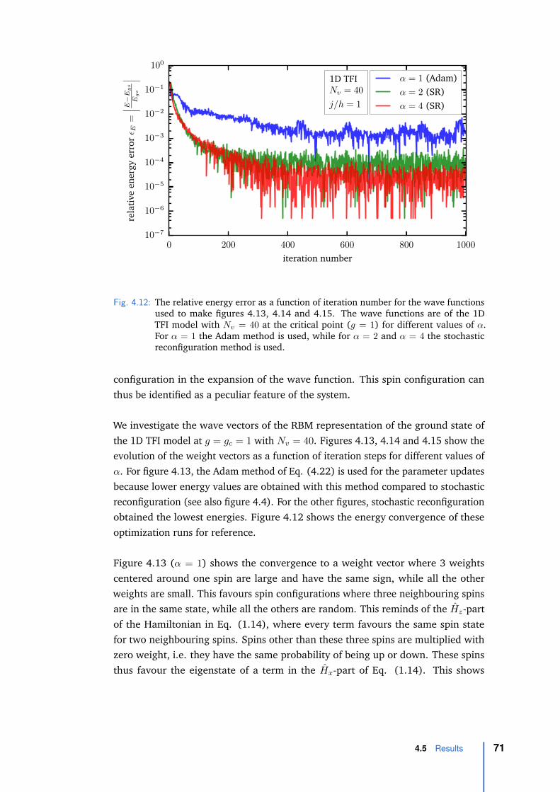
0 200 400 600 800 1000

iteration number

10−7

10−6

10−5

10−4

10−3

10−2

10−1

100

rela

tive

ener

gyer

rorε E

=∣ ∣ ∣E−Egs

Egs

∣ ∣ ∣ 1D TFINv = 40

j/h = 1

α = 1 (Adam)α = 2 (SR)α = 4 (SR)

Fig. 4.12: The relative energy error as a function of iteration number for the wave functionsused to make figures 4.13, 4.14 and 4.15. The wave functions are of the 1DTFI model with Nv = 40 at the critical point (g = 1) for different values of α.For α = 1 the Adam method is used, while for α = 2 and α = 4 the stochasticreconfiguration method is used.

configuration in the expansion of the wave function. This spin configuration canthus be identified as a peculiar feature of the system.

We investigate the wave vectors of the RBM representation of the ground state ofthe 1D TFI model at g = gc = 1 with Nv = 40. Figures 4.13, 4.14 and 4.15 show theevolution of the weight vectors as a function of iteration steps for different values ofα. For figure 4.13, the Adam method of Eq. (4.22) is used for the parameter updatesbecause lower energy values are obtained with this method compared to stochasticreconfiguration (see also figure 4.4). For the other figures, stochastic reconfigurationobtained the lowest energies. Figure 4.12 shows the energy convergence of theseoptimization runs for reference.

Figure 4.13 (α = 1) shows the convergence to a weight vector where 3 weightscentered around one spin are large and have the same sign, while all the otherweights are small. This favours spin configurations where three neighbouring spinsare in the same state, while all the others are random. This reminds of the Hz-partof the Hamiltonian in Eq. (1.14), where every term favours the same spin statefor two neighbouring spins. Spins other than these three spins are multiplied withzero weight, i.e. they have the same probability of being up or down. These spinsthus favour the eigenstate of a term in the Hx-part of Eq. (1.14). This shows

4.5 Results 71

0 200 400 600 800 1000

iteration number

0

5

10

15

20

25

30

35

wei

ght

num

berw

1 i

1D TFI, g = gc = 1, Nv = 40, Nh = 40

Fig. 4.13: The weights in the weight vector as a function of iteration step for the 1D TFI withNv = 40, α = 1 and g = 1. A red color indicates a high positive weight and a bluecolor a low negative weight. The weight vector is periodically translated such thatthe highest weight in absolute value is centered on weight 20. The weight vectorconverges to one feature centered around a few neighbouring spins. See figure4.12 for the energy convergence as a function of the iteration step.

that the representation captures both the short range features (the Hz-part of theHamiltonian) and the long-range features (the Hx-part of the Hamiltonian).

Figure 4.14 (α = 2) shows the same qualitative weight vectors in both filters. Anadditional property of these filters is that they show small, but non-zero, weightsin a broad range around the center spin (approximately 20 spins). This is what wewould intuitively expect for a system at the critical point (gc = 1), where correlationshave a long range. However, it is to be expected that the correlations appear withthe same sign, which is not the case in the left panel of figure 4.14. It needs tobe pointed out that the presence of more than one filter partially complicates theinterpretability of the weight vector, because new factors in the product of cosinehyperbolics of Eq. (4.10) appear. In this case both filters can be used to favour agiven spin configuration because they can be independently translated.

Figure 4.15 (α = 4) shows the same behaviour as figure 4.14 for two filters (filter1 and 3), but new behaviour for filters 2 and 4. These weight vectors favour spinconfigurations where two neighbouring spins have opposite spin. This feature is notreadily clear from the separate parts of the Hamiltonian of Eq. (1.14). However, theexistence of new features is to be expected because the two parts of the Hamiltoniando not commute. Furthermore, the same caveat holds for the case of two filters: it is


0 200 400 600 800 1000

iteration number

0

5

10

15

20

25

30

35

wei

ght

num

berw

1 i

0 200 400 600 800 1000

iteration number

0

5

10

15

20

25

30

35

wei

ght

num

berw

2 i

1D TFI, g = gc = 1, Nv = 40, Nh = 80

Fig. 4.14: The weights in the weight vectors as a function of iteration step for the 1D TFIwith Nv = 40, α = 2 and g = 1. A red color indicates a high positive weight and ablue color a low negative weight. The weight vectors are periodically translatedsuch that the highest weight in absolute value is centered on weight 20. Bothfilters learn a different feature of the wave function. See figure 4.12 for the energyconvergence as a function of the iteration step.

possible to favour a spin configuration by the combination of all filters, which mayhave other effects than the filters independently.

It is interesting to note from figure 4.12 that the features only become apparent whenthe energy is already low. Before the relative energy error reaches approximately1%, the weight vectors are featureless with a fluctuating distribution of weights overthe spins. When the energy is low enough, the weight vectors converge to a sharplypeaked distribution around a few spins, which monotonously decreases for spinsfurther away from the peak. It is interesting that this change in structure happensvery suddenly and when the energy has already significantly converged. Further,remember that the stochastic reconfiguration algorithm is based in imaginary-timeevolution, which means that during the optimization, the excited states present inthe initial random state are multiplied with a weight cn relative to the ground state,which is proportional to

cn ∝ exp(−t(En − Egs)), (4.69)

where En is the energy of the excited state and t is a measure for the number ofiteration steps. It is thus clear that the first excited state is the state which remainspresent for the largest amount of iteration steps (excluding the ground state) in thevariational wave function.

4.5 Results 73

0 200 400 600 800 1000

iteration number

05

101520253035

wei

ght

num

berw

1 i

0 200 400 600 800 1000

iteration number

05

101520253035

wei

ght

num

berw

2 i0 200 400 600 800 1000

iteration number

05

101520253035

wei

ght

num

berw

3 i

0 200 400 600 800 1000

iteration number

05

101520253035

wei

ght

num

berw

4 i

1D TFI, g = gc = 1, Nv = 40, Nh = 160

Fig. 4.15: The weights in the weight vectors as a function of iteration step for the 1D TFIwith Nv = 40, α = 4 and g = 1. A red color indicates a high positive weight and ablue color a low negative weight. The weight vectors are periodically translatedsuch that the highest weight in absolute value is centered on weight 20. Differentfilters learn a different feature of the wave function. See figure 4.12 for the energyconvergence as a function of the iteration step.

4.5.6 Weight histograms

The weight histograms for different values of g = h/j of the 1D TFI model withNv = 40 are shown in figure 4.16. For every subpanel, we used α = 4 and plotted thefrequency of occurrence of weights with specific values for 10 separately trained wavefunctions. The weight histograms give information about how many parametersare needed to represent the wave function. Broad histograms indicate that manyparameters are non-vanishing and are reminiscent of highly correlated systems. Theplots in figure 4.16 show a broadening of the histogram when going from high tolow values of g. This can be appreciated physically. For g � 1, the ground state willlie close to the eigenstate with smallest eigenvalue of the Hx-contribution to theHamiltonian of Eq. (1.14)

Hx = −hNv∑

i=1

σix. (4.70)

Because this part does not contain interactions between spins, the eigenstate of thisoperator with minimal eigenvalue can be found by taking the direct product of theeigenstates with minimal eigenvalue of every term in Eq. (4.70) separately. Here, wewill use the notation |↑x,y,z〉 (|↓x,y,z〉) for the eigenstates

∣∣sx,y,z = 12

⟩(∣∣sx,y,z = −1

2

⟩)


−0.10 −0.05 0.00 0.05 0.10

weight value

02468

10121416

freq

.of

occu

rren

ce

g = 0.5

−0.10 −0.05 0.00 0.05 0.10

weight value

0102030405060

freq

.of

occu

rren

ce

g = 1

−0.10 −0.05 0.00 0.05 0.10

weight value

020406080

100120140

freq

.of

occu

rren

ce

g = 1.5

−0.10 −0.05 0.00 0.05 0.10

weight value

020406080

100120140

freq

.of

occu

rren

ce

g = 2

1D TFI, Nv = 40, Nh = 160

Fig. 4.16: Histogram of the weight values for the 1D TFI model with Nv = 40 and α = 4 fordifferent values of the coupling g. The histograms are composed of all the weightsof 10 independently trained wave functions. Broad histograms indicate that thewave function is more difficult to train because many variational parameterscontribute non-trivially to the wave function.

of the operator σx,y,z in order to make the notations lighter. Using Eqs. (1.7) and(1.8), the eigenstate |↑x〉 minimizing −hσx is

|↑x〉 = |↑z〉+ |↓z〉 → −hσx |↑x〉 = −h |↑x〉 . (4.71)

The direct product of these states for every spin yields the wave function |Ψx〉minimizing Eq. (4.70):

|Ψx〉 =∑

S|s1zs

2z...s

Nvz 〉 → −h

∑

i

σix |Ψx〉 = −hNv |Ψx〉 . (4.72)

This is the state where every Ψ(S;W) is equal to one. It is clear from Eq. (4.10) thatthis is the state where every weight is zero.

The other extreme situation, g � 1, corresponds with the eigenstate with smallesteigenvalue of the Hz-part of the Hamiltonian of Eq. (1.14)

Hz = −j∑

〈i,k〉

σizσkz . (4.73)

4.5 Results 75

The eigenstate with minimal eigenvalue of one term −jσ1zσ

2z in the sum is either∣∣↑1z↑2z

⟩or∣∣↓1z↓2z

⟩as can be seen from

−jσ1zσ

2z

∣∣↑1z↑2z⟩

= −j∣∣↑1z↑2z

⟩and − jσ1

zσ2z

∣∣↓1z↓2z⟩

= −j∣∣↓1z↓2z

⟩. (4.74)

The eigenstates with minimal eigenvalue of Eq. (4.73) are thus∣∣↑1z↑2z ... ↑Nv

z

⟩and∣∣↓1z↓2z ... ↓Nv

z

⟩or a linear combination of them. The eigenstate |Ψz〉 which is invariant

under the spin flip operator of Eq. (4.11) is

|Ψz〉 =∣∣↑1z↑2z ... ↑Nv

z

⟩+∣∣↓1z↓2z ... ↓Nv

z

⟩→ −j

∑

〈i,k〉

σizσkz |Ψz〉 = −jNv(Nv − 1)

2|Ψz〉 .

(4.75)The weights in Eq. (4.10) should now attain values such that Ψ(S;W) is one for theconfigurations where all the spins are up or all the spins are down in the σz-basisand zero for all the other configurations. One solution is that all the weights havethe same (high) value. However, multiple (non-trivial) solutions can exist. It is clearhowever that, in order to enforce that all spin have approximately the same value,all the weights should contribute a non-zero value.

4.5.7 Correlations

1 2 3 4 5 6 7 8

number of filters α

10−8

10−7

10−6

10−5

10−4

10−3

10−2

rela

tive

ener

gyer

rorε E

=∣ ∣ ∣E−Egs

Egs

∣ ∣ ∣ 1D TFINv = 40

g =0.5g =1g =1.5g =2

Fig. 4.17: The relative energy errors corresponding to the RBM states in figure 4.18. Themodel is a 1D TFI with Nv = 40. The errors are shown as a function of the numberof filters α and the coupling g.


0 5 10 15 20

distance between spins r

0.0

0.2

0.4

0.6

0.8

1.0

G(r

)g = 0.5

0 5 10 15 20


0.0

0.2

0.4

0.6

0.8

1.0

G(r

)

g = 1

0 5 10 15 20


0.0

0.2

0.4

0.6

0.8

1.0

G(r

)

g = 1.5

0 5 10 15 20


0.0

0.2

0.4

0.6

0.8

1.0

G(r

)

g = 2

1D TFI, Nv = 40

α = 1α = 2

α = 4α = 5

α = 6α = 7

α = 8

Fig. 4.18: The correlation function as defined in Eq. (4.76) for different values of g andα in a 1D TFI model with Nv = 40. This figure shows the long-range order forg < 1, the non-trivial long-range correlations for g = 1 and the disorder for g > 1.States with a large amount of correlations (either long-range order or criticalcorrelations) are more difficult to represent with RBM states. The non-visiblelines are due to overlap with other lines. See figure 5.7 for an investigation of thecorrelation function close to the critical point.

After convergence, the wave functions can be used to calculate expectation values ofphysical observables. One central observable is the spin-spin correlation functionG(r), defined as

G(r) = 〈σizσi+rz 〉. (4.76)

Note that this observable does not depend on the index i due to translation invariance.The correlation function describes the probability that two spins which are r indicesapart are aligned. When long-range order is present in the system, the correlationfunction for r →∞ converges to

G(r)r→∞

=⟨σiz⟩ ⟨σi+∞z

⟩=⟨σiz⟩2, (4.77)

where we used the fact that 〈σiz〉 = 〈σjz〉 for every j due to translational invariance.That this relation holds can be appreciated by the fact that spins which are infinitelyfar apart attain values independently of each other because there is no direct inter-action between them. The correlation function can be corrected for this long-rangebehaviour, yielding the connected spin-spin correlation function C(r)

C(r) = G(r)−⟨σiz⟩2

= 〈(σiz −⟨σiz⟩)(σi+rz −

⟨σiz⟩)〉. (4.78)

4.5 Results 77

Eq. (4.76) and Eq. (4.78) are both valid measures to measure the correlationspresent in a system. Eq. (4.76) provides both the non-trivial correlations (arisingfrom direct interactions) and the systematic correlations due to long-range order. Eq.(4.76) only provides the non-trivial part of the correlations. We will argue belowthat Eq. (4.76) is the most natural way of providing the correlation function in thecontext of RBM quantum states.

The correlation functions G(r) of Eq. (4.76) for the TFI are displayed in figure 4.18.The corresponding relative energy errors are depicted in figure 4.17 for reference.For g = 0.5, g = 1.5 and g = 2, we see that the correlation function does notchange appreciably with increasing α. The energy errors are low for every valueof α, compared to g = 1. This supports the results of section 4.5.6: ground stateswith a disordered character are easy to represent with a RBM wave function. Forg = 0.5, the correlations are for the most part of a long-range character. This isharder to represent than no correlations at all, but the RBM proves to be able torepresent them with one filter. For g = 1, we see that the correlation function is notwell-represented for α < 5. This behaviour is logical considering that g = 1 is thecritical point, where the non-trivial correlations are the largest.

0 5 10 15 20 25 30 35 40

weight index i

−1.0

−0.5

0.0

0.5

1.0

wei

ghtwi g = 0.5

0 5 10 15 20 25 30 35 40

weight index i

−1.0

−0.5

0.0

0.5

1.0

wei

ghtwi g = 1

0 5 10 15 20 25 30 35 40

weight index i

−1.0

−0.5

0.0

0.5

1.0

wei

ghtwi g = 1.5

0 5 10 15 20 25 30 35 40

weight index i

−1.0

−0.5

0.0

0.5

1.0

wei

ghtwi g = 2

1D TFI, Nv = 40, Nh = 160

Fig. 4.19: The weight vectors for different values of g for a 1D TFI with Nv = 40 and α = 4.The weight vectors are centered such that the highest weight is in the middleof the weight vector. A horizontal line at wi = 0 is added for clarity. Note thequalitative relation between the weight vectors and the correlation functions infigure 4.18.

Figure 4.19 shows the four weight vectors of an RBM with α = 4 for the same valuesof g as in figure 4.18. The highest value of a weight vector can be seen as a referencevalue: because the weight vector is multiplied with the spin configuration via the


inner product, the spin corresponding to the highest weight is enforced in a certainstate (up or down), and the other weights determine the behaviour of the otherspins with respect to this reference spin. It is expected that for disordered states,the spins are fairly independent, resulting in a weight vector with a short range ofnon-zero weights around the reference weight. This behaviour is seen in figure 4.19.For the state at g = 1 we see that the weights decay to zero with increasing distancefrom the highest weight, although much slower than when g > 1. This reflects thelong-range correlations present at criticality. Finally, for g = 0.5, we see that theweights decrease for increasing distance from the highest weight, but converge toa non-zero value. This reflects the long-range order in the ground state of systemswith g < 1: the spins far away from the reference spin should still have a tendencyto align with the reference spin.

We thus find that the qualitative behaviour of the weight vector is the same as thebehaviour of the spin-spin correlation function defined in Eq. (4.76). Althougha qualitative connection between the weight vectors and the correlation functioncan be made, the weight vectors show behaviour which is more complex than thecorrelation function. For example, in the case where g = 0.5, the weight vectorsare globally non-zero, but the weight vectors show slowly varying fluctuationsaround zero. Another feature are the fluctuations between positive and negativeweights around the highest weight. These features arise from the fact that theexpansion coefficient of the wave function in Eq. (4.3) is a complex product ofcosine hyperbolics, which can lead for example to the cancellation of effects foundin the weight vectors.

4.5 Results 79

5Finite-size scaling for theTransverse Field Ising model

In chapter 4, the quality of the ground-state wave functions was evaluated by meansof energy related measures. For instance, the relative energy error of the resolvedground states with respect to the (quasi)-exact ground state energies (section 4.5.1)and the energy fluctuations of the determined states (section 4.5.3) were measured.Energy-related measures have their limitations to fully determine the quality ofa resolved ground state, especially near criticality. This can be understood byconsidering the energy gap ∆E , defined as the energy difference between the groundand the first excited state

∆E = E1 − Egs, (5.1)

where E1 is the energy of the first excited state and Egs is the energy of the groundstate. The energy gap tends to zero for systems approaching the critical point [84].This makes the use of the energy as a convergence measure questionable. In a finitesystem with linear dimension L, it can be proven that the energy gap ∆E(L) isnon-zero, and scales as [88]:

∆E(L) ∝ L−z, (5.2)

with z the dynamical critical exponent. This fact is the motivation to look beyondenergy-related measures. Other properties of the ground state give complementaryinformation about the trustworthiness of the numerical results. For this reason, wewill study the phase transition in the ground state of the one-dimensional transversefield Ising system. We determine properties of the ground states with the aid ofthe method described in chapter 4. By studying the finite-size scaling of the phasetransition in the TFI model, we can get information about the critical exponents,observables and response functions of the system. This information is relevant as itstudies the most correlated wave functions attainable by the TFI model, which areexpected to be most difficult to describe.

5.1 The finite-size scaling method

Finite-size scaling originates from statistical physics, where it is used for studyingclassical phase transitions. It can be directly translated to quantum mechanics, by

81

the analogy between the nature of the phase transition in classical and quantumsystems [13]. In this section, we will introduce the finite-size scaling method.

It is well known that selected observables of many-body physical systems displaypower law behaviour near the critical point [3, 84]. This behaviour can be capturedby the so-called critical exponents of the system: these are the exponents of thepower laws describing the observables. We will use the notation of [97], where gstands for the control variable of the model, i.e. the parameter of the system whichinduces the phase transition. In the TFI model g = h/j. Furthermore, gc is the valueof the control variable at which the phase transition occurs. The definitions of theobservables and the critical exponents are as follows:

• Correlation length ξ (critical exponent ν):

ξ ∝ |g − gc|−ν (for g ≈ gc). (5.3)

The correlation length ξ defines the length scale of the connected spin-spincorrelation function defined in Eq. (4.78):

C(r) =exp(−r/ξ)rd−2+η

, (5.4)

with η another critical exponent (often referred to as anomalous exponent) andd the dimension of the system.

• Order parameter 〈|sz|〉 (critical exponent β):

〈|sz|〉 ∝ (gc − g)β (for g . gc). (5.5)

the quantity 〈|sz|〉 is defined in Eq. (4.62).

• Order parameter susceptibility χs (critical exponent γ):

χs =

(∂〈|sz|〉∂h‖

)

h‖→0

∝ |g − gc|−γ (for g ≈ gc), (5.6)

where h‖ is an external magnetic field in the z-direction. We refrain fromsimulating the TFI model with an external magnetic field in the z-direction, i.e.h‖ = 0. However, χs can be obtained from the spin-spin correlation functionC(r) of Eq. (4.78) at h‖ = 0 by integrating it over all the spin sites (see forexample [98]):

χs ∝Nv∑

i=1

C(i). (5.7)

82 Chapter 5 Finite-size scaling for the Transverse Field Ising model

Phase transitions happen in principle only in the thermodynamic limit, i.e. forNv →∞. In simulations, one is restricted to systems with a finite size. We thus needa way to connect the observables in finite systems to those in the thermodynamiclimit. A convenient way to do this is via the finite-size scaling method. This methodassumes that data has been collected for systems in a range of values of the controlparameter (including the transition point) and in a range of system sizes. The firststep in the finite-size scaling analysis is writing a certain observable near the criticalpoint, for example the order parameter, in terms of the correlation length:

〈|sz|〉 ∝ ξ−β/ν , (5.8)

where we make use of Eqs. (5.5) and (5.3). For infinite systems, the correlationlength ξ diverges to infinity near criticality. For finite systems however, the correlationlength is bounded by the size of the system. This implies that the order parametercannot diverge polynomially near gc but will go smoothly to zero when approachinggc. To describe this behaviour, the order parameter of Eq. (5.8) is expressed asfollows:

〈|sz|〉 ∝ ξ−β/νs0z(L/ξ), (5.9)

where ξ is the correlation length the system would have in the thermodynamiclimit and s0

z is a function which is constant when L � ξ (such that the scalingrelation of Eq. (5.8) holds) and is equal to (L/ξ)−β/ν when L < ξ. Eq. (5.9) nowexplicitly describes how 〈|sz|〉 scales with system size. However, it depends on theunknown correlation length. To eliminate the correlation length (and bring back thedependence on the deviation from the critical point) from Eq. (5.9), we define thefollowing new scaling function sz(x)

sz(x) = xβs0z(x

ν). (5.10)

Using expression (5.10) in Eq. (5.9), we get

〈|sz|〉 ∝ L−β/ν sz(L1/ν(g − gc)), (5.11)

which now explicitly depends on the system size L and the control variable g. We canmake the following observations. First, when we measure 〈|sz|〉Lβ/ν as a functionof g, the curves for the different system sizes all cross at the same value gc becausethe argument of sz is zero. This makes it possible to determine gc, given the criticalexponents are known. Second, the critical exponents (and gc) can be determined.This can be done by noting that when plotting 〈|sz|〉Lβ/ν versus L1/ν(g − gc), thecurves for all the different system sizes should coincide. This property is called datacollapse. Note that this only holds in the vicinity of the critical point, as the scalinganalysis is only valid in this region. By varying the critical exponents and the criticaltransverse field, the appropriate values of the exponents and the critical point are

5.1 The finite-size scaling method 83

found when the different curves collapse. The above analysis can be carried out forthe other observables in Eqs. (5.3) and Eq. (5.6), yielding similar relationships.

We now wish to define a quantitative measure to evaluate the quality of the datacollapse. To perform the data collapse and find the critical exponents and theirerrors, we use the AutoScale.py routine from [99]. This routine defines a measure Qfor the quality of the data collapse as in [100]:

Q =1

N

∑

g,L

(y(g, L)− Y (g, L))2

(dy(g, L))2 + (dY (g, L))2. (5.12)

Here, N is the number of (g, L)-pairs in the dataset. Furthermore, y(g, L) is themeasured scaled value of the observable for a (g, L)-pair (e.g. in the case of the orderparameter y(g, L) = 〈|sz|〉Lβ/ν) and dy(g, L) is the measured standard deviation ony(g, L). Lastly, Y (g, L) is the scaling function at (g, L) (e.g. Y (g, L) = sz(L

1/ν(g−gc))in the case of the order parameter (see Eq. (5.11))), and dY (g, L) is the standarddeviation on it.

Because the scaling function Y (g, L) is unknown, it is estimated from the data pointsy(g, L) in the following way. Given (g, L), those data points (labeled by (g′, L′)) areselected for which L′1/ν(g′ − gc) lies within a predefined range from L1/ν(g − gc).With these values, a linear least squares fit is performed. Then, Y (g, L) is thefunction value of this linear fit at the point labeled by (g, L). The standard deviationdY (g, L) is determined from the error on the fit. When the scaling is performedwith the wrong critical exponents, there is no data collapse and the linear fit will bepoor. This will result in a high value of the quantity Q. When the data does collapseon a single curve, Y (g, L) will be close to y(g, L) and Q will be small. The correctcritical exponents can thus be extracted by minimizing Q. This is done by usingthe iterative optimization method of Nelder and Mead [101]. Since Q measuresthe deviation from the curve Y divided by the errors on measurement and curve,it resembles a χ2 test. This implies that Q should be close to one when the correctcritical exponents are used. The error on the critical exponents is found by theQ + 1 method, which means that the error is defined as the range of values thecritical exponents could have such that Q does not deviate more than one unit fromthe minimal value. This measure is motivated by the resemblance with the χ2 test,where the error is determined by the surface of χ2 + 1-values in the parameter space.This can be brought back to the fact that the deviations in the definition of χ2 (or inthis case Q) are normalized by the error on it.

Of course, the data collapse only holds in a specific range around the critical valueof the control variable. In turn, the collapse is only good (as determined by Q ≈ 1)for this small range of control variables. Because there is no good way to determine


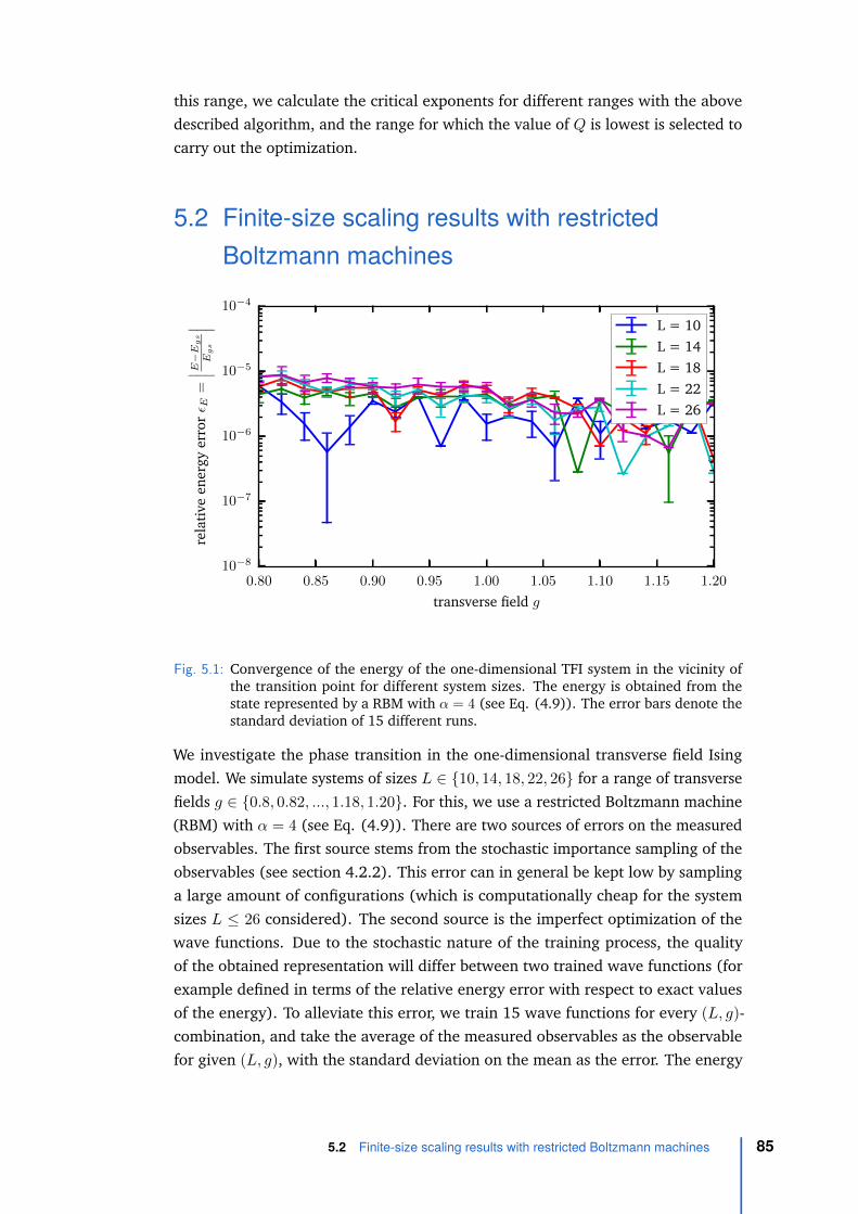
this range, we calculate the critical exponents for different ranges with the abovedescribed algorithm, and the range for which the value of Q is lowest is selected tocarry out the optimization.

5.2 Finite-size scaling results with restrictedBoltzmann machines

0.80 0.85 0.90 0.95 1.00 1.05 1.10 1.15 1.20

transverse field g

10−8

10−7

10−6

10−5

10−4

rela

tive

ener

gyer

rorε E

=∣ ∣ ∣E−Egs

Egs

∣ ∣ ∣ L = 10L = 14L = 18L = 22L = 26

Fig. 5.1: Convergence of the energy of the one-dimensional TFI system in the vicinity ofthe transition point for different system sizes. The energy is obtained from thestate represented by a RBM with α = 4 (see Eq. (4.9)). The error bars denote thestandard deviation of 15 different runs.

We investigate the phase transition in the one-dimensional transverse field Isingmodel. We simulate systems of sizes L ∈ {10, 14, 18, 22, 26} for a range of transversefields g ∈ {0.8, 0.82, ..., 1.18, 1.20}. For this, we use a restricted Boltzmann machine(RBM) with α = 4 (see Eq. (4.9)). There are two sources of errors on the measuredobservables. The first source stems from the stochastic importance sampling of theobservables (see section 4.2.2). This error can in general be kept low by samplinga large amount of configurations (which is computationally cheap for the systemsizes L ≤ 26 considered). The second source is the imperfect optimization of thewave functions. Due to the stochastic nature of the training process, the qualityof the obtained representation will differ between two trained wave functions (forexample defined in terms of the relative energy error with respect to exact valuesof the energy). To alleviate this error, we train 15 wave functions for every (L, g)-combination, and take the average of the measured observables as the observablefor given (L, g), with the standard deviation on the mean as the error. The energy

5.2 Finite-size scaling results with restricted Boltzmann machines 85

convergence of the different (L, g)-combinations is depicted in figure 5.1. We see thatthe relative energy error of all the (L, g)-combinations is lower than 10−5, implyingthat the determined wave function can be expected to be close the ground state.

5.2.1 Magnetization histograms

−1.0 −0.5 0.0 0.5 1.0

magnetization per spin mz

123456789

10

−lo

g(P

(mz))

g = 0.8

−1.0 −0.5 0.0 0.5 1.0


3.43.63.84.04.24.44.64.85.0

−lo

g(P

(mz)) g = 1.04

−1.0 −0.5 0.0 0.5 1.0


3.0

3.5

4.0

4.5

5.0

5.5

−lo

g(P

(mz)) g = 1.08

−1.0 −0.5 0.0 0.5 1.0


2345678

−lo

g(P

(mz)) g = 1.2

Fig. 5.2: The negative logarithm of the distribution of the magnetization in the 1D TFI modelfor different transverse field strengths g and L = 30. The change from a doublewell to a single well is clearly visible and resembles the behaviour of the classicaltwo-dimensional Ising model.

As a first measure, we can investigate the symmetry breaking of the phase transition.For brevity, we will denote sz ≡

∑Nvi=1 σ

iz

Nvfrom now on. We measure the probability

of the different possible magnetization values for fixed system size and differenttransverse fields. The probability is defined as

P (mz) =∑

{S}

δ (mz − 〈S | sz | S〉)Ψ(S;W)∗Ψ(S;W)

〈Ψ |Ψ〉 , (5.13)

where |Ψ〉 is the state for which the probability distribution is defined. Because theσz-basis of Eq. (1.11) is an eigenbasis of the operator sz, 〈S | sz | S〉 will yield aneigenvalue of sz. Thus, mz is a variable which can take on all possible eigenvaluesof sz.

To make the connection with the classical two-dimensional Ising model, we calculatethe negative logarithm of the probability distribution. This should represent a freeenergy-like function, as it is defined in the same way as the free energy (as a functionof magnetization) is defined in classical statistical physics. The measured values for


system size L = 30 for different transverse field strengths g are depicted in figure5.2. We see the same qualitative behaviour as the classical Ising model. For h ≥ j,the transverse field part of the Hamiltonian dominates and the ground state in theσz-basis converges to a superposition of disordered states (see also section 4.5.6).This corresponds to the disordered states found in the high-temperature range ofthe classical Ising model, i.e. the supercritical states. The negative logarithm of themagnetization distribution corresponds to the one found in the classical case, i.e.a single well centered around zero. For h ≤ j, the Ising part of the Hamiltoniandominates and the ground state converges to the ground state of the Ising part Hz ofthe Hamiltonian in Eq. (1.14) (i.e. comparable with the subcritical behaviour of theclassical Ising model). The negative logarithm of the magnetization now shows adouble well, with the two lowest points at a non-zero magnetization differing fromeach other only in the sign. At g ≈ 1, there is a cross-over between the two differentprofiles. This shows the symmetry breaking in the low transverse field region, alsopresent in the classical Ising model at T < Tc. Figure 5.2 also shows the finite-sizeeffects of the magnetization: the magnetization stays non-zero when g is slightlylarger than 1. The consequence is that the magnetization converges smoothly tozero for g → ∞ in finite systems. In infinite systems, the magnetization is alwayszero in the supercritical region (g > gc) (see for example [3]).

5.2.2 Binder cumulant

0.80 0.85 0.90 0.95 1.00 1.05 1.10 1.15 1.20

transverse field g

0.20

0.25

0.30

0.35

0.40

0.45

0.50

0.55

0.60

0.65

Bin

der

cum

ulan

tU

=1−〈m

4 z〉

3〈m

2 z〉2

L = 10L = 14L = 18L = 22L = 26

−10 −5 0 5 10

(g − 0.999)L1.04

0.2

0.3

0.4

0.5

0.6

0.7

U

data collapse

Fig. 5.3: The Binder cumulant for the TFI model. The inset shows the scaled Binder cumulantaccording to the found critical exponents.

The Binder cumulant U quantifies the deviation of the order parameter probabilitydistribution P (mz) of Eq. (5.13) from a Gaussian probability distribution [102]. It is


10 15 20 25 30

mean of lattice sizes L used for intersection

0.96

0.97

0.98

0.99

1.00

crit

ical

poin

tg c

extr

acte

dfr

omin

ters

ecti

on

fit to crossing meansexact critical point gc = 1

mean of distribution with standard error

Fig. 5.4: Violin plot of the crossing of the Binder cumulant between two subsequent systemsizes. The violins denote the probability distribution of the crossing from ourbootstrap sample obtained via kernel density estimation. The x-axis denotes theaverage of the system sizes used to determine each crossing ((L2 − L1)/2). Thecurve is a power law least squares fit to the means of the distributions, resulting ingcrossc = −6.65L−2.31 + 0.997.

defined as the ratio of the fourth-order cumulant Q4 and the second-order cumulantQ2 of the magnetization distribution P (mz) times −1/3:

U = − Q4

3Q2= 1− 〈m4

z〉3〈m2

z〉2(5.14)

The distribution of the magnetization P (mz) scales with L as:

P (mz, L) = LyP (mzLx, ξ/L), (5.15)

for general x, y and with P (mzLx, ξ/L) a dimensionless scaling function. The

moments 〈mkz〉 of this distribution scale as follows

〈mkz〉 =

∫ 1

−1mkzP (mz, L)dmz

=

∫ 1

−1mkzL

yP (mzLx, ξ/L)dmz

= Lx(−k−1)Ly∫ Lx

−Lx

(mzLx)kP (mzL

x, ξ/L)d(mzLx)

= Lx(−k−1)LyFk(ξ/L).

(5.16)


The function Fk(ξ/L) now only depends on ξ/L because the dependence on mz isintegrated out. The normalization (k = 0) ensures that x = y because it cannotdepend on L. Using this form for the Binder cumulant, we get the following scalingrelation (for g ≈ gc) [103]:

U = 1− L−4xF4(ξ/L)

3L−4xF2(ξ/L)2= U((g − gc)L1/ν), (5.17)

where U((g − gc)L1/ν) is a new scaling function defined from the scaling functionsof the moments of the magnetization distribution. One can see from Eq. (5.17)that the Binder cumulant does not explicitly scale with system size. For g = gc,the Binder cumulant for different system sizes coincides. This makes the Bindercumulant popular for the determination of the critical point gc as it can be foundwithout any scaling optimization and independently of the critical exponents. TheBinder cumulant for different (g, L)-combinations is shown in figure 5.3. We seethat the curves cross at a single point, determining the critical point gc. To findthe exact intersections, an interpolation is performed for every curve on the plot.From this interpolation, the crossing points between the curves of two subsequentvalues of L can be determined. To determine the errors on the intersection, abootstrap method is performed. For every (g, L)-pair, the different measurementsof the Binder cumulant are sampled with replacement to generate a subset of themeasurements (recall that we have 15 measurements per (g, L)-pair). From thesesubsets, the curves are determined and the intersections measured. This procedureis repeated with different subsets of measurements and yields a distribution ofthe crossing points. The results of this analysis are shown in figure 5.4. This plotshows the distributions of the crossings of the curves of two subsequent systemsizes. The distributions are obtained from the bootstrapping procedure estimatedvia kernel density estimation [104]. To obtain the crossings of the last two points,we performed extra simulations for L ∈ {22, 26, 30} and g ∈ {0.98, 0.985, ..., 1.015}to obtain a denser sampling of points in the vicinity of the critical point, whichincreases the quality of the interpolations needed to find the crossing points. This isrequired due to the sensitivity of the crossing point to the interpolation. From themeasured distribution, we determine the mean and the standard deviation. Fromthe analysis, we see that the extracted critical points are slightly underestimated,although a systematic convergence towards the real critical point may be possiblejudging from the plot (this behaviour is typical for the crossing points of the Bindercumulant [105]). A power law function can be fitted to these measurements via theleast squares method. We get the following functional form for the crossings gcrossc

gcrossc (L) = −6.65L−2.31 + 0.997. (5.18)

In the thermodynamic limit (L→∞), we find that the function gcrossc (L) approachesthe value 0.997(4) where the error is measured from the covariance matrix obtained


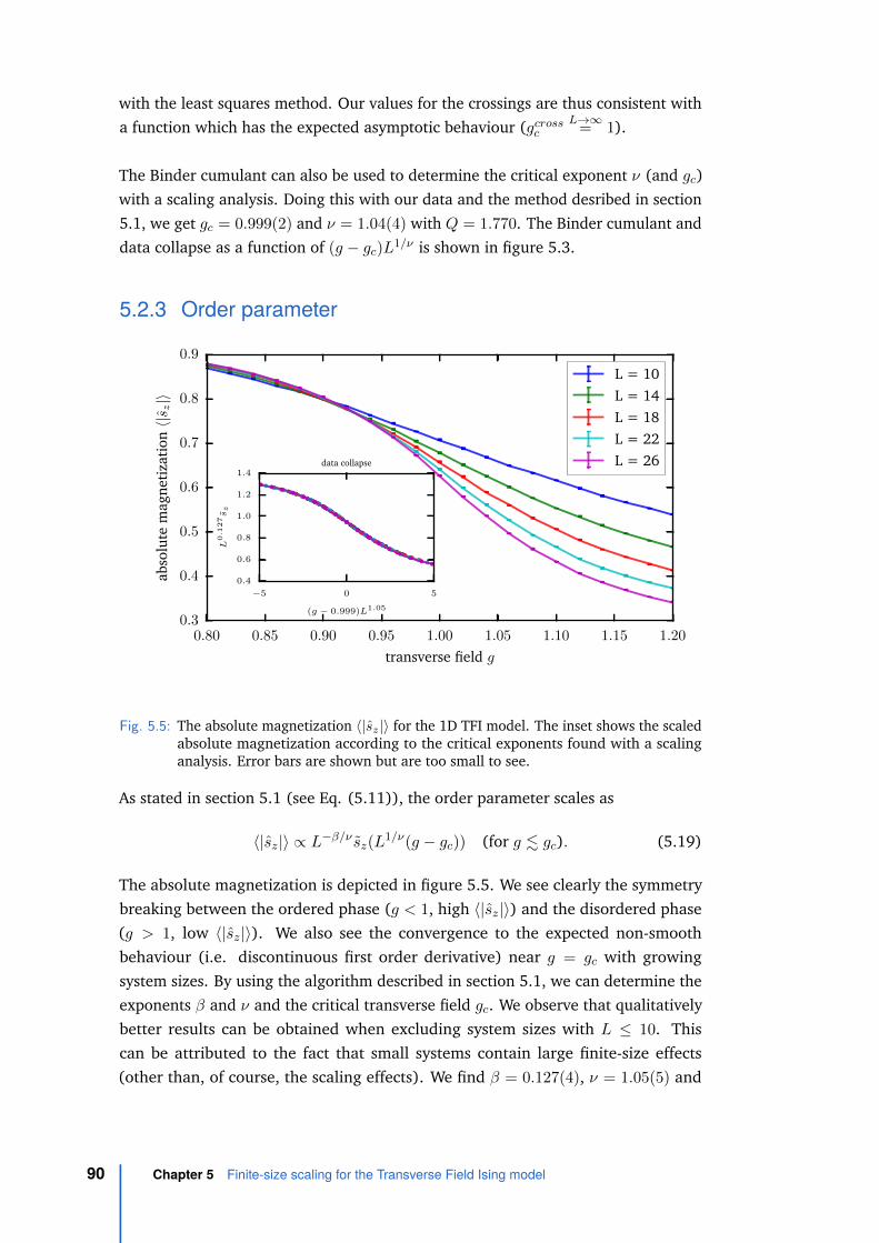
with the least squares method. Our values for the crossings are thus consistent witha function which has the expected asymptotic behaviour (gcrossc

L→∞= 1).

The Binder cumulant can also be used to determine the critical exponent ν (and gc)with a scaling analysis. Doing this with our data and the method desribed in section5.1, we get gc = 0.999(2) and ν = 1.04(4) with Q = 1.770. The Binder cumulant anddata collapse as a function of (g − gc)L1/ν is shown in figure 5.3.

5.2.3 Order parameter

0.80 0.85 0.90 0.95 1.00 1.05 1.10 1.15 1.20

transverse field g

0.3

0.4

0.5

0.6

0.7

0.8

0.9

abso

lute

mag

neti

zati

on〈|s

z|〉

L = 10L = 14L = 18L = 22L = 26

−5 0 5

(g − 0.999)L1.05

0.4

0.6

0.8

1.0

1.2

1.4

L0.1

27sz

data collapse

Fig. 5.5: The absolute magnetization 〈|sz|〉 for the 1D TFI model. The inset shows the scaledabsolute magnetization according to the critical exponents found with a scalinganalysis. Error bars are shown but are too small to see.

As stated in section 5.1 (see Eq. (5.11)), the order parameter scales as

〈|sz|〉 ∝ L−β/ν sz(L1/ν(g − gc)) (for g . gc). (5.19)

The absolute magnetization is depicted in figure 5.5. We see clearly the symmetrybreaking between the ordered phase (g < 1, high 〈|sz|〉) and the disordered phase(g > 1, low 〈|sz|〉). We also see the convergence to the expected non-smoothbehaviour (i.e. discontinuous first order derivative) near g = gc with growingsystem sizes. By using the algorithm described in section 5.1, we can determine theexponents β and ν and the critical transverse field gc. We observe that qualitativelybetter results can be obtained when excluding system sizes with L ≤ 10. Thiscan be attributed to the fact that small systems contain large finite-size effects(other than, of course, the scaling effects). We find β = 0.127(4), ν = 1.05(5) and


gc = 0.999(2). The quality of the collapse as measured by Q (see Eq. (5.12)) is inthis case Q = 1.133. The collapse is shown in the inset of figure 5.5.

The fact that the order parameter tends to 1 for g → 0 is additional evidence for thefact that we indeed obtain the ground-state wave function because the magnetizationvanishes for the excited states. The absolute magnetization never completely vanishes,even not when the magnetization does, but for a linear combination of all excitedstates it will never raise above 0.5.

5.2.4 Order parameter susceptibility

0.80 0.85 0.90 0.95 1.00 1.05 1.10 1.15 1.20

transverse field g

0.0

0.5

1.0

1.5

2.0

2.5

3.0

3.5

orde

rpa

ram

eter

resp

onse

func

tion

χs L = 10

L = 14L = 18L = 22L = 26

−5 0 5

(g − 0.981)L1.0

0.00

0.05

0.10

0.15

0.20

L−

0.7

3χs

data collapse

Fig. 5.6: The susceptibility of the order parameter χs for the 1D TFI model. The insetshows the scaled order parameter susceptibility according to the extracted criticalexponents.

The susceptibility of the order parameter scales as

χs =∂〈|sz|〉∂h

∝ Lγ/νχs(L1/ν(g − gc)) (for g ≈ gc). (5.20)

The order parameter susceptibility is displayed as a function of the transverse field gin figure 5.6. Also these curves follow the expected behaviour of a response function.The response is low for values of the control variable far from the critical point. Atg = gc, a peak in the response function is observed, reflecting the large amount offluctuations at this point. The finite-size behaviour is seen in the growth of the peakvalue of the susceptibility, which should diverge in the thermodynamic limit. Thefinite size scaling analysis yields γ = 0.73(3), ν = 1.0(3) and gc = 0.981(7). Thequality of the proposed data collapse as determined by Eq. (5.12) is Q = 0.555. It is


interesting that the error on ν is quite large compared to the other errors. However,when cross-checking with the value of ν determined in the scaling analyses of theorder parameter and the Binder cumulant, all are consistent with each other. Thevalue of gc, on the other hand, shows a deviation compared with the value obtainedin the scaling of the order parameter. However, the values are consistent withinthree times the error. We stress again that the error estimate as determined by Eq.(5.12) is scheme dependent and might be underestimated.

5.2.5 Integral of correlation function

The correlation function at the critical point is defined as

G(r) ∝ 1

rd−2+η, (5.21)

as can be seen from Eq. (4.76) with ξ →∞. The integral of the correlation functionshould thus scale as ∫ L

0G(r)dr ∝ L2−η. (5.22)

Since the order parameter susceptibility is defined as the integral of the correlationfunction (see Eq. (5.7)), we see that the following relation holds

2− η = γ/ν, (5.23)

which is one of the scaling relations of the critical exponents [3]. Although Eq.(5.23) determines η from the knowledge of ν and γ, it is still interesting to computeη from Eq. (5.22) as a cross-check. Furthermore, Eq. (5.22) only depends on η. Thismeans that deriving η does not depend on the values of the other critical exponents,as is the case for the scaling analysis described in section 5.1, where two criticalexponents and gc are involved in the optimization. The exponent η is determined byfitting with the least squares method a polynomial function y = axb− c to the valuesof the correlation function integral at the critical point. The exponent in the integralof the correlation function is found to be 2− η = 0.753(4), which yields η = 0.247(4).We also see that the scaling relation (5.23) is consistent in our analysis.

5.2.6 Comparison with other work

The finite-size scaling analysis of the 1D TFI model has been analysed in the contextof exact diagonalization (ED) in Ref. [106] and matrix product states (MPS) in Ref.[107]. In the case of ED, the critical exponents were not explicitly determined viaa scaling analysis. Rather, the behaviour of the observables when scaled with thecritical exponents of the 2D classical Ising model was investigated in a qualitative


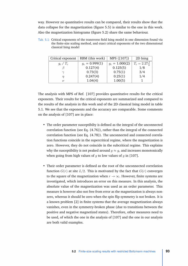
way. However no quantitative results can be compared, their results show that thedata collapse for the magnetization (figure 5.5) is similar to the one in this work.Also the magnetization histograms (figure 5.2) share the same behaviour.

Tab. 5.1: Critical exponents of the transverse field Ising model in one dimension found viathe finite-size scaling method, and exact critical exponents of the two dimensionalclassical Ising model

Critical exponent RBM (this work) MPS ([107]) 2D Isinggc / Tc gc = 0.999(1) gc = 1.000(2) Tc = 2.27Jkβ 0.127(4) 0.125(5) 1/8γ 0.73(3) 0.75(1) 3/4η 0.247(4) 0.25(1) 1/4ν 1.04(4) 1.00(5) 1

The analysis with MPS of Ref. [107] provides quantitative results for the criticalexponents. Their results for the critical exponents are summarized and compared tothe results of the analysis in this work and of the 2D classical Ising model in table5.1. We see that the exponents and the accuracy are comparable. Some commentson the analysis of [107] are in place:

• The order parameter susceptibilty is defined as the integral of the unconnectedcorrelation function (see Eq. (4.76)), rather than the integral of the connectedcorrelation function (see Eq. (4.78)). The unconnected and connected correla-tion functions coincide in the supercritical regime, where the magnetization iszero. However, they do not coincide in the subcritical regime. This explainswhy the susceptibility is not peaked around g ≈ gc and increases monotonicallywhen going from high values of g to low values of g in [107].

• Their order parameter is defined as the root of the unconnected correlationfunction G(r) at site L/2. This is motivated by the fact that G(r) convergesto the square of the magnetization when r →∞. However, finite systems areinvestigated, which introduces an error on this measure. In this analysis, theabsolute value of the magnetization was used as an order parameter. Thismeasure is however also not free from error as the magnetization is always non-zero, whereas it should be zero when the spin flip symmetry is not broken. It isa known problem [2] in finite systems that the average magnetization alwaysvanishes, even in the symmetry-broken phase (due to transitions between thepositive and negative magnetized states). Therefore, other measures need tobe used, of which the one in the analysis of [107] and the one in our analysisare both valid examples.


100 101


10−2

10−1

100

G(r

)

Nv = 120

g = 0.96g = 0.98g = 1g = 1.02g = 1.04

100 101 102


10−2

10−1

100

G(r

)

g = 1 Nv = 40Nv = 60Nv = 80Nv = 100

1D TFI, α = 4

Fig. 5.7: (Unconnected) correlation functions G(r) of the TFI in the vicinity of the criticalpoint determined from RBM wave functions with α = 4. Left: the correlationfunction for Nv = 120 around the critical point. Right: the correlation function atthe critical point for different system sizes.

Special attention is given to the behaviour of correlations in [107]. More specifically,they show the correlation function for g ∈ {0.96, 0.98, ..., 1.04} and L = 120 and forg = gc = 1 and L ∈ {20, 40, ..., 120}. For comparison, we plot the same functionsobtained with the RBM approach in figure 5.7. The same behaviour as in [107] isobserved. We see from this figure the expected behaviour of the correlation functionG(r). For g < 1 the correlation function levels off due to long-range order for whichG(r) is not corrected. For g > 1 the correlation function curves downwards, denotingthe exponential decrease to zero. At g = 1 the correlation function is a straightline for r < L/2, denoting the power law behaviour of the correlation function atcriticality (see Eq. (5.4)).

Furthermore, [107] calculates the correlation length as defined by the secondmoment correlation length ξ2

ξ2 =1

q1

(2S(0)

S(q1)− 2

)1/2

, (5.24)

where q1 is the smallest allowed wave vector (i.e. q1 = 2πL ) and S(q) is the static

structure factor, or the fourier transform of the connected correlation function

S(q) =

Nv∑

r=1

exp(iqr)C(r). (5.25)


1.00 1.05 1.10 1.15 1.20

transverse field strength g

0.0

0.5

1.0

1.5

2.0

norm

aliz

edse

cond

mom

.co

rr.

leng

thξ 2/L

L = 10L = 14L = 18L = 22L = 26

0 1 2 3 4 5

(g − 0.999)L1.04

0.0

0.2

0.4

0.6

0.8

1.0

L−

0.9

8ξ2

data collapse

Fig. 5.8: The second moment correlation length ξ2 of the 1D TFI for different system sizes Land transverse fields g. The inset shows the data collapse according to the measuredcritical exponents. Error bars are shown but are too small to see.

This definition is proportional to the second moment of the connected correlationfunction:

ξ2 =1

q1

(2S(0)

S(q1)− 2

)1/2

∝∑Nv

r=1 r2C(r)

∑Nvr=1C(r)

. (5.26)

Note that Ref. [107] claims that the second moment correlation function is equal to

ξ2 =1

q1

(2S(0)

S(q1)− 2

)1/(2−z−η)

, (5.27)

where z is the dynamical critical exponent (see introduction to this chapter). How-ever, other literature [88] shows that Eq. (5.24) is the correct form. Note that thesecond moment correlation length is only well-defined when the correlation functiongoes to zero when r →∞ (hence the use of the connected correlation function). Be-cause only the unconnected correlation function is easily accessible in finite systems,we calculate the second moment correlation length only in the supercritical regime(where G(r) coincides with C(r)). The second moment correlation function is shownin figure 5.8. We see that the second moment correlation length normalized to thesystem size grows when approaching gc = 1 and attains the same value, independentof system size, at g = 1. Scaling can be performed according to the ansatz

ξ2 = Lξ2((g − gc)L1/ν), (5.28)


where ξ2 is a dimensionless scaling function. From this ansatz, the exponent ν andthe critical point gc can be determined. We find from our data ν = 1.04(8) andgc = 0.999(2) with the quality Q = 0.807 (see Eq. (5.12)).

The fact that the correlation function at g = 1 decays polynomially with distance(see figure 5.7), and, equivalently, that the correlation length approaches the systemsize at g = 1 (see figure 5.8) provides the most compelling evidence that theobtained states are indeed the ground state. It can be proven that states whichare a linear combination of the ground state and the excited states always have afinite correlation length, depending on the weight of the excited states in the linearcombination [84].

5.2.7 Conclusion

The results of our finite-size scaling analysis are summarized in table 5.1. For thecritical exponents which are measured more than once, we reported the one withthe smallest error. We already saw that these critical exponents are consistent witheach other. The transverse field Ising model in one dimension belongs to the sameuniversality class as the two-dimensional classical Ising model (see section 4.4.1) andthus should have the same critical exponents. This is found (within the errorbars) inour analysis. The fact that the correlation function decays polynomially with distanceand the fact that the magnetization is non-vanishing provides further evidence thatthe obtained states are indeed the ground states.

It is clear that the restricted Boltzmann representation of the wave functions ofquantum spin systems is able to represent the ground states at quantum criticalpoints. This proves that the correlations induced by the hidden nodes are wellsuitable to describe the high degree of correlations in quantum systems at a criticalpoint, with a reasonable amount of computational resources.


6Conclusion and outlook

6.1 Conclusion

This thesis explored how machine learning can be used to solve problems in many-body physics. Chapters 1 and 2 introduced many-body physics and machine learningrespectively. Examining the concepts introduced in these two chapters resulted inchapter 3, where we outlined the connection between these two seemingly unrelatedfields. Specifically, high-dimensional systems and correlations are features on whichthese two fields heavily hinge. This provided the motivation to investigate howthese fields can benefit from each other. Chapter 3 further provided examples ofhow concepts from many-body physics can be used in machine learning and howmachine learning techniques can be used in many-body physics.

In chapter 4 we investigated in detail how restricted Boltzmann machines (RBM)(introduced in section 2.3.3) can be used as an ansatz for the wave function ofstrongly-correlated quantum spin systems. For this, we followed closely the workof [57]. After describing the model in the context of quantum spin systems insection 4.1, we describe how to optimize the model to represent the ground state ofquantum spin systems in section 4.2. Theoretical results and the relation to othermethods used to find the ground state and energy of quantum spin systems aredescribed in section 4.3. The ansatz and the optimization procedure described insections 4.1 and 4.2 were implemented in a computer code and the results wereinvestigated in section 4.5. The different learning schemes described in section 4.2.2were compared on different models (the transverse field Ising and antiferromagneticHeisenberg models, described in section 4.4). It was found that the Adam method[66] and the stochastic reconfiguration method [68] are capable of attaining thelowest energies. However, from the 2D antiferromagnetic Heisenberg model, it wasfound that the stochastic reconfiguration method surpassed the Adam method interms of energy minimization. In sections 4.5.2 and 4.5.3 we investigated how thequality of the ground state (measured in terms of relative energy error and relativeenergy fluctuations) depends on the number of parameters (or hidden nodes) in theRBM ansatz. The quality of the ground state increases with increasing number ofparameters, in line with the variational principle and the universal approximationtheorem (see section 2.3.3). In section 4.5.2, we also investigated the quality of theground state with increasing number of degrees of freedom. The RBM is capable of

97

representing states of systems with an arbitrary number of degrees of freedom, evenimproving on the relative energy error for larger system sizes. In sections 4.5.5 and4.5.6, we investigated whether the internal representation (i.e. the weights of theRBM) can shed light on the physics of the ground state we model. For this, we usedthe 1D transverse field Ising model. It is found that the filters of the RBM representto some extent what we would expect from the Hamiltonian of which we model theground state, although some features are present which are not to be expected fromthe Hamiltonian. The weight histograms of the RBM at different magnitudes of thetransverse field shed light on the correlations present in the ground state. It is foundthat ground states with long-range order have significantly more non-zero weightsthan ground states which do not exhibit long-range order. Finally, in section 4.5.7we calculate explicitly the correlation functions for the obtained ground states atdifferent magnitudes of the transverse field and different numbers of filters. It isfound that the ground state at criticality is the hardest to represent, which is to beexpected from the fact that the correlations become scale-free.

In chapter 5 we investigated the quality of the ground states obtained with the RBMapproach in more detail. Instead of only using the energy as a measure for thequality of the ground state, other observables should also be investigated to be ableto claim that the RBM is a good representation of the ground state. Especially atcriticality this is important due to the fact that the first excited states have an energyclose to the ground-state energy. We investigated the quality of the ground state ofthe 1D TFI near criticality by performing a finite-size scaling analysis to determinethe critical exponents β, γ, η and ν (see section 5.1 for their definitions) and thecritical point gc. In section 5.2.2 we calculate the Binder cumulant and determinethe critical point gc from the crossing of the curves of the Binder cumulant as afunction of g for different system sizes. The crossings show a systematic increasetowards the exact critical point, and are consistent with a power law behaviourwhich asymptotically converges to gc = 1. Performing a data collapse yields a criticalpoint and critical exponent ν which are consistent (within the errors) with the exactvalues. Data collapse of the order-parameter (section 5.2.3) and the order-parametersusceptibility (section 5.2.4) yield a critical point and critical exponents β, γ and νwhich are also consistent (within the errors) with the exact values. The integral ofthe correlation function (section 5.2.5) yields the critical exponent η, again consistentwith the exact value. The results are compared with results obtained with othermethods (exact diagonalization [106] and matrix product states [107]) in section5.2.6. Both qualitatively and quantitatively comparable results were found.

98 Chapter 6 Conclusion and outlook

6.2 Outlook

As for the analysis of this thesis specifically, we can formulate the following improve-ments and optimizations. First, a more thorough study of the optimal hyperparame-ters (i.e. the parameters associated with the learning scheme, such as the learningrate) of the optimization schemes can be performed and compared between learningschemes. For example, is there an optimization scheme for which the results onlyweakly depend on the choice of hyperparameters compared to other schemes? Thisquestion is relevant as the true representational power of the RBM can only beaccessed via a well-performing optimization procedure. Another question is whetheralgorithms which do not depend on the gradient of the energy but only on energyvalues (such as the method of Nelder and Mead [101] or genetic algorithms) workfor the determination of ground state-wave functions. If this is the case, the compu-tational cost of the RBM method would be significantly reduced as the determinationof the gradients dominate the computational cost of the optimization algorithm (seesection 4.2). It was recently shown [108] that the success of gradient-free methodsdiminishes with the number of parameters to be optimized. This makes the successof the approach questionable for large systems. However, the approach can still befeasible for small systems.

Second, the RBM approach could be extended to include parameters describinglong-range order. Section 4.5.6 described how long-range order is encoded in theRBM by setting many weights to a non-zero value. However, long-range order isa systematic effect, for which it is not natural to model with explicit correlationsbetween the spins described by the weights of the RBM. If the systematic effect canbe described by a separate mechanism, the weights of the RBM would serve forcorrelations not described by this systematic effect, and would more naturally reflectthe connected correlation function.

Third, the critical exponents which we did not measure in our finite-size scalinganalysis could be investigated. These are the exponent of the control variablesusceptibility α, the dynamical critical exponent z, and the critical exponent δ ofthe dependence of the magnetization on the longitudinal magnetic field h‖. Theexponent α could have been readily measured in our analysis, however it requiresthe determination of a derivative via finite-difference methods, which holds largestatistical errors. The determination of the dynamical critical exponent requirestime-dependent wave functions and the exponent δ requires the inclusion of alongitudinal magnetic field in the simulations. Both features were not considered,but the information extracted from them can give further insight in the validity ofthe obtained wave functions.

6.2 Outlook 99

Promising results were found in chapters 4 and 5. However, due to the novelcharacter of the field, there remain a lot of challenges for the RBM method to solveproblems in quantum many-body physics. Some examples are

• To what extent can the internal representation be used to extract informationon properties of the system?

• Can RBMs represent all classes of systems faithfully (e.g. topological states)?

• Can the RBM ansatz be used to represent the excited states of Hamiltonians?

• Can the RBM ansatz include different symmetries of Hamiltonians?

• Are there other learning schemes which outperform stochastic reconfiguration?

• How exactly does the RBM approach relate to other methods (in constructionand in accuracy)?

• Is there an extension to the RBM approach such that it can describe infinitesystems?

A somewhat more general question is whether other machine learning models canrepresent quantum many-body wave functions and how they compare to the RBMmethod. Examples are other types of neural networks such as convolutional neuralnetworks or generative adversarial networks (see section 2.3.4) or deep Boltzmannmachines (which is the deep variant of Boltzmann machines, i.e. a stack of multipleBoltzmann machines). Preliminary studies have already been caried out [59, 60],but a thorough investigation is needed to establish the optimal model to approximatewave functions of quantum many-body systems.

100

Nederlandse samenvatting

Systemen met veel vrijheidsgraden zijn een van de meest complexe fysische sys-temen. Een manier om inzicht te krijgen in deze veeldeeltjessystemen is door deconnectie te maken tussen de microscopische vrijheidsgraden en de macroscopischevariabelen. Hoe deze connectie formeel gemaakt kan worden, wordt beschreven inde theorie van statistische fysica en de kwantumveeldeeltjestheorie. Hoewel dezetheorieën een exacte beschrijving geven van de connectie tussen de microscopie ende macroscopie van een systeem, blijkt het in de praktijk echter vaak nodig om be-naderingen en numerieke simulaties uit te voeren. Recente ontwikkelingen brachteneen nieuwe manier naar voren die dergelijke benaderingen kan maken: machinaalleren. Technieken uit machinaal leren hebben de eigenschap dat ze de connectiekunnen maken tussen microscopische variabelen (bijvoorbeeld pixels in een foto)en macroscopische concepten (bijvoorbeeld het object dat op een foto staat). Dezeeigenschap maakt technieken uit machinaal leren interessant voor toepassingen inveeldeeltjestheorie omdat het net die connectie is die we willen maken in fysischesystemen.

In deze thesis gaan we dieper in op het gebruik van machinaal leren voor veeldeelt-jessystemen. In hoofdstuk 1 en 2 worden respectievelijk veeldeeltjesfysica en machi-naal leren geïntroduceerd. De concepten besproken in deze twee hoofdstukkenworden gecombineerd in hoofdstuk 3, waar beschreven wordt hoe machinaal lerengebruikt kan worden in veeldeeltjesfysica, maar ook hoe veeldeeltjesfysica gebruiktkan worden in machinaal leren. In hoofdstuk 4 gaan we dieper in op een van detoepassingen van machinaal leren in veeldeeltjesfysica: het gebruik van restrictedBoltzmann machines (RBM) als ansatz voor de golffunctie van sterk gecorreleerdekwantum spin systemen. In eerste instantie volgen we het werk van [57]. De resul-taten die we bekomen zijn in lijn met de resultaten van [57]. Vervolgens gaan weverder in op de interne representatie van de RBM en gaan we na of dit strookt met defysische realiteit. We vinden kwalitatieve verbanden tussen de interne representatievan de RBM en de fysische fenomenen in het systeem, zoals lange dracht orde enkorte dracht interacties. In hoofdstuk 5 gaan we dieper in op de kwaliteit van deRBM-representatie van grondtoestanden van kwantum spin systemen. In hoofdstuk4 werd de energie gebruikt (in de vorm van relatieve fout op exacte waarden offluctuaties) als maat voor de kwaliteit van de gevonden grondtoestand. Vooral in

101

de buurt van kritische punten worden deze maten minder betekenisvol omdat hetenergieverschil tussen de eerste aangeslagen toestand en de grondtoestand kleinwordt. Verder is de regio rond het kritisch punt moeilijk te beschrijven door de grotehoeveelheid aan correlaties. Als test voor de kwaliteit van RBM-representaties doenwe een finite-size scaling analyse van het eendimensionaal transvers veld Ising model.Hiermee vinden we de theoretisch voorspelde resultaten voor de kritische exponen-ten β, γ, η en ν en voor het kritisch punt gc. Dit betekent dat de RBM-representatiewel degelijk de juiste grondtoestanden representeert. We vergelijken onze analysemet de beschikbare analyses in de literatuur en vinden dat onze resultaten consistentzijn met die bekomen aan de hand van andere methodes.

102

Science popularization

To popularize science, I did a short talk about how machine learning can be usedto find the connection between microscopic degrees of freedom and macroscopicproperties of many-body systems. This talk was brought by me on a public event,organised by VVN (Vereniging voor Natuurkunde). The aim of the event was toprovide a stage for master’s students doing scientific studies to present the work theydid for their master’s thesis to the general public in an accessible way. The talk is inDutch and is aimed at high school students in their final year. The talk can be foundat https://www.youtube.com/watch?v=hYqYae3JTAE.

103

https://www.youtube.com/watch?v=hYqYae3JTAE

Bibliography

1R. J. Baxter, Exactly solved models in statistical mechanics (Elsevier, 2016) (cit. on p. 2).

2J. Thijssen, Computational physics (Cambridge university press, 2007) (cit. on pp. 3, 4,93).

3H. Gould and J. Tobochnik, Statistical and thermal physics: with computer applications(Princeton University Press, 2010) (cit. on pp. 3, 60, 82, 87, 92).

4A. M. Belaza, K. Hoefman, J. Ryckebusch, et al., “Statistical physics of balance theory”,PLoS one 12, e0183696 (2017) (cit. on p. 3).

5T. Vicsek, A. Czirók, E. Ben-Jacob, I. Cohen, and O. Shochet, “Novel type of phasetransition in a system of self-driven particles”, Physical Review Letters 75, 1226 (1995)(cit. on p. 3).

6Z. Wang, C. T. Bauch, S. Bhattacharyya, et al., “Statistical physics of vaccination”, PhysicsReports 664, 1–113 (2016) (cit. on p. 3).

7A. Engel, Statistical mechanics of learning (Cambridge University Press, 2001) (cit. onp. 3).

8B. H. Bransden, Quantum mechanics (Pearson Education, 2000) (cit. on pp. 3, 4, 45).

9S. Sirca and M. Horvat, Computational methods for physicists: compendium for students(Springer Science & Business Media, 2012) (cit. on p. 4).

10M. P. Nightingale and C. J. Umrigar, Quantum Monte Carlo methods in physics andchemistry, 525 (Springer Science & Business Media, 1998) (cit. on p. 4).

11M. A. Nielsen and I. L. Chuang, Quantum computation and quantum information (Cam-bridge university press, 2010) (cit. on p. 8).

12H. de Raedt and A. Lagendijk, “Monte Carlo simulation of quantum statistical latticemodels”, Physics Reports 127, 233–307 (1985) (cit. on pp. 8, 9).

13M. Suzuki, “Relationship between d-Dimensional Quantal Spin Systems and (d+1)-Dimensional Ising SystemsEquivalence, Critical Exponents and Systematic Approximantsof the Partition Function and Spin Correlations”, Progress of Theoretical Physics 56,1454–1469 (1976) (cit. on pp. 9, 11, 82).

14M. Suzuki, “Generalized Trotter’s formula and systematic approximants of exponential op-erators and inner derivations with applications to many-body problems”, Communicationsin Mathematical Physics 51, 183–190 (1976) (cit. on p. 9).

15T Mitchell, Machine Learning (McGraw Hill, 1997), p. 2 (cit. on p. 13).

105

http://dx.doi.org/10.1143/PTP.56.1454

http://dx.doi.org/10.1143/PTP.56.1454

16S. Lloyd, “Least squares quantization in PCM”, IEEE Transactions on Information Theory28, 129–137 (1982) (cit. on p. 13).

17P. A. Gagniuc, Markov Chains: From Theory to Implementation and Experimentation (JohnWiley & Sons, 2017) (cit. on p. 13).

18D. Silver, J. Schrittwieser, K. Simonyan, et al., “Mastering the game of go without humanknowledge”, Nature 550, 354–359 (2017) (cit. on p. 13).

19G. Hinton, L. Deng, D. Yu, et al., “Deep neural networks for acoustic modeling in speechrecognition: The shared views of four research groups”, IEEE Signal Processing Magazine29, 82–97 (2012) (cit. on p. 13).

20S. J. Park, B. Bae, J. Kim, and M. Swaminathan, “Application of machine learning foroptimization of 3-D integrated circuits and systems”, IEEE Transactions on Very LargeScale Integration (VLSI) Systems 25, 1856–1865 (2017) (cit. on p. 13).

21I. Kononenko, “Machine learning for medical diagnosis: history, state of the art andperspective”, Artificial Intelligence in medicine 23, 89–109 (2001) (cit. on p. 13).

22R. J. Bolton and D. J. Hand, “Statistical fraud detection: A review”, Statistical Science,235–249 (2002) (cit. on p. 13).

23W. Huang, Y. Nakamori, and S.-Y. Wang, “Forecasting stock market movement directionwith support vector machine”, Computers & Operations Research 32, 2513–2522 (2005)(cit. on p. 13).

24Y. LeCun, C. Cortes, and C. Burges, “MNIST handwritten digit database”, AT&T Labs[Online]. Available: http://yann. lecun. com/exdb/mnist (2010) (cit. on p. 15).

25I. Goodfellow, Y. Bengio, A. Courville, and Y. Bengio, Deep learning, Vol. 1 (MIT pressCambridge, 2016) (cit. on p. 16).

26K. Pearson, “LIII. On lines and planes of closest fit to systems of points in space”, TheLondon, Edinburgh, and Dublin Philosophical Magazine and Journal of Science 2, 559–572 (1901) (cit. on p. 17).

27L. v. d. Maaten and G. Hinton, “Visualizing data using t-SNE”, Journal of Machine LearningResearch 9, 2579–2605 (2008) (cit. on p. 18).

28C. Cortes and V. Vapnik, “Support-vector networks”, Machine Learning 20, 273–297(1995) (cit. on p. 18).

29M. A. Aizerman, “Theoretical foundations of the potential function method in patternrecognition learning”, Automation and Remote Control 25, 821–837 (1964) (cit. onp. 19).

30J. Carrasquilla and R. G. Melko, “Machine learning phases of matter”, Nature Physics 13,431–434 (2017) (cit. on pp. 21, 35).

31K. Hornik, M. Stinchcombe, and H. White, “Multilayer feedforward networks are universalapproximators”, Neural Networks 2, 359–366 (1989) (cit. on p. 22).

32J. J. Hopfield, “Neural networks and physical systems with emergent collective computa-tional abilities”, Proceedings of the National Academy of Sciences 79, 2554–2558 (1982)(cit. on p. 28).

33D. O. Hebb, The organization of behavior: A neuropsychological theory (Psychology Press,2005) (cit. on p. 28).

106

34D. H. Ackley, G. E. Hinton, and T. J. Sejnowski, “A learning algorithm for Boltzmannmachines”, in Readings in computer vision (Elsevier, 1987), pp. 522–533 (cit. on p. 28).

35L. P. Kadanoff, “Notes on Migdal’s recursion formulas”, Annals of Physics 100, 359–394(1976) (cit. on p. 29).

36P. Mehta and D. J. Schwab, “An exact mapping between the variational renormalizationgroup and deep learning”, arXiv preprint arXiv:1410.3831 (2014) (cit. on p. 29).

37H. W. Lin, M. Tegmark, and D. Rolnick, “Why does deep and cheap learning work sowell?”, Journal of Statistical Physics 168, 1223–1247 (2017) (cit. on p. 30).

38D. Liu, S.-J. Ran, P. Wittek, et al., “Machine learning by two-dimensional hierarchicaltensor networks: A quantum information theoretic perspective on deep architectures”,arXiv preprint arXiv:1710.04833 (2017) (cit. on p. 30).

39Y. Levine, D. Yakira, N. Cohen, and A. Shashua, “Deep Learning and Quantum Entangle-ment: Fundamental Connections with Implications to Network Design.”, arXiv preprintarXiv:1704.01552 (2017) (cit. on p. 31).

40P. Baldi, P. Sadowski, and D. Whiteson, “Searching for exotic particles in high-energyphysics with deep learning”, Nature Communications 5 (2014) (cit. on p. 31).

41J. VanderPlas, A. J. Connolly, Ž. Ivezic, and A. Gray, “Introduction to astroML: Machinelearning for astrophysics”, in Intelligent data understanding (cidu), 2012 conference on(IEEE, 2012), pp. 47–54 (cit. on p. 31).

42Y. Fujimoto, K. Fukushima, and K. Murase, “Methodology study of machine learningfor the neutron star equation of state”, arXiv preprint arXiv:1711.06748 (2017) (cit. onp. 32).

43R. Utama, W.-C. Chen, and J. Piekarewicz, “Nuclear charge radii: density functionaltheory meets Bayesian neural networks”, Journal of Physics G: Nuclear and ParticlePhysics 43, 114002 (2016) (cit. on p. 32).

44L.-G. Pang, K. Zhou, N. Su, et al., “An equation-of-state-meter of quantum chromody-namics transition from deep learning”, Nature Communications 9, 210 (2018) (cit. onp. 32).

45R. H. Swendsen and J.-S. Wang, “Nonuniversal critical dynamics in Monte Carlo simula-tions”, Physical Review Letters 58, 86–88 (1987) (cit. on p. 33).

46J. Liu, Y. Qi, Z. Y. Meng, and L. Fu, “Self-learning Monte Carlo method”, Physical ReviewB 95, 041101 (2017) (cit. on p. 33).

47A. Morningstar and R. G. Melko, “Deep learning the Ising model near criticality”, arXivpreprint arXiv:1708.04622 (2017) (cit. on p. 34).

48Z. Liu, S. P. Rodrigues, and W. Cai, “Simulating the Ising Model with a Deep ConvolutionalGenerative Adversarial Network”, arXiv preprint arXiv:1710.04987 (2017) (cit. on p. 34).

49P. Broecker, J. Carrasquilla, R. G. Melko, and S. Trebst, “Machine learning quantumphases of matter beyond the fermion sign problem”, Scientific Reports 7, 8823 (2017)(cit. on p. 34).

50L. Wang, “Discovering phase transitions with unsupervised learning”, Physical Review B94, 195105 (2016) (cit. on p. 35).

107

http://dx.doi.org/10.1103/PhysRevLett.58.86

http://dx.doi.org/10.1103/PhysRevB.94.195105


51K. Ch’ng, J. Carrasquilla, R. G. Melko, and E. Khatami, “Machine Learning Phases ofStrongly Correlated Fermions”, Physical Review X 7, 031038 (2017) (cit. on p. 35).

52E. P. van Nieuwenburg, Y.-H. Liu, and S. D. Huber, “Learning phase transitions byconfusion”, Nature Physics 13, 435–439 (2017) (cit. on p. 36).

53M. J. S. Beach, A. Golubeva, and R. G. Melko, “Machine learning vortices at the Kosterlitz-Thouless transition”, Physical Review B 97, 045207 (2018) (cit. on p. 36).

54A. Shrikumar, P. Greenside, and A. Kundaje, “Learning Important Features ThroughPropagating Activation Differences”, in International conference on machine learning(2017), pp. 3145–3153 (cit. on p. 36).

55J. T. Springenberg, A. Dosovitskiy, T. Brox, and M. Riedmiller, “Striving for simplicity:The all convolutional net”, arXiv preprint arXiv:1412.6806 (2014) (cit. on p. 36).

56P. Ponte and R. G. Melko, “Kernel methods for interpretable machine learning of orderparameters”, Physical Review B 96, 205146 (2017) (cit. on p. 36).

57G. Carleo and M. Troyer, “Solving the quantum many-body problem with artificial neuralnetworks”, Science 355, 602–606 (2017) (cit. on pp. 36, 37, 39, 62, 69, 97, 101).

58Y. Nomura, A. S. Darmawan, Y. Yamaji, and M. Imada, “Restricted Boltzmann machinelearning for solving strongly correlated quantum systems”, Physical Review B 96, 205152(2017) (cit. on pp. 37, 69).

59H. Saito, “Solving the Bose–Hubbard model with machine learning”, Journal of thePhysical Society of Japan 86, 093001 (2017) (cit. on pp. 37, 100).

60H. Saito and M. Kato, “Machine learning technique to find quantum many-body groundstates of bosons on a lattice”, Journal of the Physical Society of Japan 87, 014001 (2017)(cit. on pp. 37, 100).

61I. Glasser, N. Pancotti, M. August, I. D. Rodriguez, and J. I. Cirac, “Neural-NetworkQuantum States, String-Bond States, and Chiral Topological States”, Physical Review X 8,011006 (2018) (cit. on pp. 37, 58, 59).

62X. Glorot and Y. Bengio, “Understanding the difficulty of training deep feedforwardneural networks”, in Proceedings of the thirteenth international conference on artificialintelligence and statistics (2010), pp. 249–256 (cit. on pp. 44, 67).

63W. K. Hastings, “Monte Carlo sampling methods using Markov chains and their applica-tions”, Biometrika 57, 97–109 (1970) (cit. on p. 46).

64J. Duchi, E. Hazan, and Y. Singer, “Adaptive subgradient methods for online learning andstochastic optimization”, Journal of Machine Learning Research 12, 2121–2159 (2011)(cit. on p. 47).

65M. D. Zeiler, “ADADELTA: an adaptive learning rate method”, arXiv preprint arXiv:1212.5701(2012) (cit. on p. 48).

66D. P. Kingma and J. Ba, “Adam: A method for stochastic optimization”, arXiv preprintarXiv:1412.6980 (2014) (cit. on pp. 48, 97).

67G. Goh, “Why Momentum Really Works”, Distill (2017) 10.23915/distill.00006 (cit.on pp. 48, 65).

68S. Sorella, “Green Function Monte Carlo with Stochastic Reconfiguration”, PhysicalReview Letters 80, 4558–4561 (1998) (cit. on pp. 48, 97).

108

http://dx.doi.org/10.1103/PhysRevX.7.031038


http://dx.doi.org/10.23915/distill.00006

http://dx.doi.org/10.23915/distill.00006



69S.-C. T. Choi and M. A. Saunders, “Algorithm 937: MINRES-QLP for symmetric and her-mitian linear equations and least-squares problems”, ACM Transactions on MathematicalSoftware (TOMS) 40, 16 (2014) (cit. on p. 51).

70M. M. Wolf, F. Verstraete, M. B. Hastings, and J. I. Cirac, “Area laws in quantum systems:mutual information and correlations”, Physical Review Letters 100, 070502 (2008) (cit.on p. 54).

71M. B. Hastings, “An area law for one-dimensional quantum systems”, Journal of StatisticalMechanics: Theory and Experiment 2007, P08024 (2007) (cit. on p. 54).

72D.-L. Deng, “Machine Learning Bell Nonlocality in Quantum Many-body Systems”,arXiv:1710.04226 (2017) (cit. on p. 55).

73D.-L. Deng, X. Li, and S. Das Sarma, “Machine learning topological states”, PhysicalReview B 96, 195145 (2017) (cit. on p. 55).

74J. Chen, S. Cheng, H. Xie, L. Wang, and T. Xiang, “Equivalence of restricted Boltzmannmachines and tensor network states”, Physical Review B 97, 085104 (2018) (cit. onpp. 55, 58).

75H. Lin, J. Gubernatis, H. Gould, and J. Tobochnik, “Exact diagonalization methods forquantum systems”, Computers in Physics 7, 400–407 (1993) (cit. on p. 56).

76E. S. Coakley and V. Rokhlin, “A fast divide-and-conquer algorithm for computing thespectra of real symmetric tridiagonal matrices”, Applied and Computational HarmonicAnalysis 34, 379–414 (2013) (cit. on p. 56).

77S. R. White, “Density matrix formulation for quantum renormalization groups”, PhysicalReview Letters 69, 2863–2866 (1992) (cit. on p. 56).

78U. Schollwöck, “The density-matrix renormalization group in the age of matrix productstates”, Annals of Physics 326, 96–192 (2011) (cit. on p. 56).

79S. Rommer and S. Ostlund, “A class of ansatz wave functions for 1D spin systems andtheir relation to DMRG”, Physical Review B 55, 2164 (1997) (cit. on p. 57).

80J. Eisert, “Entanglement and tensor network states”, arXiv preprint arXiv:1308.3318(2013) (cit. on p. 58).

81N. Schuch, M. M. Wolf, F. Verstraete, and J. I. Cirac, “Simulation of Quantum Many-BodySystems with Strings of Operators and Monte Carlo Tensor Contractions”, Physical ReviewLetters 100, 040501 (2008) (cit. on p. 58).

82R. Orús, “A practical introduction to tensor networks: Matrix product states and projectedentangled pair states”, Annals of Physics 349, 117–158 (2014) (cit. on p. 58).

83P. Pfeuty, “The one-dimensional Ising model with a transverse field”, Annals of Physics57, 79–90 (1970) (cit. on p. 59).

84S. Sachdev, Quantum phase transitions (Wiley Online Library, 2007) (cit. on pp. 60, 81,82, 96).

85A. Dutta, G. Aeppli, B. K. Chakrabarti, et al., “Quantum phase transitions in transversefield spin models: From statistical physics to quantum information”, arXiv preprintarXiv:1012.0653 (2010) (cit. on p. 60).

109







86N. D. Mermin and H. Wagner, “Absence of ferromagnetism or antiferromagnetism inone-or two-dimensional isotropic Heisenberg models”, Physical Review Letters 17, 1133(1966) (cit. on p. 62).

87E. Manousakis, “The spin-½ Heisenberg antiferromagnet on a square lattice and itsapplication to the cuprous oxides”, Reviews of Modern Physics 63, 1–62 (1991) (cit. onp. 62).

88A. W. Sandvik, “Computational studies of quantum spin systems”, in Aip conferenceproceedings, Vol. 1297, 1 (AIP, 2010), pp. 135–338 (cit. on pp. 62, 81, 95).

89L. Bottou, “Large-scale machine learning with stochastic gradient descent”, in Proceedingsof compstat’2010 (Springer, 2010), pp. 177–186 (cit. on p. 62).

90B. Bauer, L. Carr, H. G. Evertz, et al., “The ALPS project release 2.0: open source softwarefor strongly correlated systems”, Journal of Statistical Mechanics: Theory and Experiment2011, P05001 (2011) (cit. on p. 64).

91C. Hamer, “Finite-size scaling in the transverse Ising model on a square lattice”, Journalof Physics A: Mathematical and General 33, 6683 (2000) (cit. on pp. 64, 65, 68, 70).

92A. W. Sandvik, “Finite-size scaling of the ground-state parameters of the two-dimensionalHeisenberg model”, Physical Review B 56, 11678–11690 (1997) (cit. on pp. 64, 66, 68,70).

93S. Al-Assam, S. R. Clark, C. J. Foot, and D. Jaksch, “Capturing long range correlationsin two-dimensional quantum lattice systems using correlator product states”, PhysicalReview B 84, 205108 (2011) (cit. on p. 68).

94L. Tagliacozzo, G. Evenbly, and G. Vidal, “Simulation of two-dimensional quantum systemsusing a tree tensor network that exploits the entropic area law”, Physical Review B 80,235127 (2009) (cit. on p. 68).

95F Mezzacapo, N Schuch, M Boninsegni, and J. I. Cirac, “Ground-state properties ofquantum many-body systems: entangled-plaquette states and variational Monte Carlo”,New Journal of Physics 11, 083026 (2009) (cit. on p. 69).

96M. Lubasch, J. I. Cirac, and M.-C. Bañuls, “Algorithms for finite projected entangled pairstates”, Physical Review B 90, 064425 (2014) (cit. on p. 69).

97T. R. Kirkpatrick and D. Belitz, “Exponent relations at quantum phase transitions withapplications to metallic quantum ferromagnets”, Physical Review B 91, 214407 (2015)(cit. on p. 82).

98M. E. Fisher, “The theory of equilibrium critical phenomena”, Reports on Progress inPhysics 30, 615 (1967) (cit. on p. 82).

99O. Melchert, “Autoscale.py - A program for automatic finite-size scaling analyses: A user’sguide”, arXiv preprint arXiv:0910.5403 (2009) (cit. on p. 84).

100J. Houdayer and A. K. Hartmann, “Low-temperature behavior of two-dimensional Gaus-sian Ising spin glasses”, Physical Review B 70, 014418 (2004) (cit. on p. 84).

101J. A. Nelder and R. Mead, “A simplex method for function minimization”, The ComputerJournal 7, 308–313 (1965) (cit. on pp. 84, 99).

102K. Binder, “Critical Properties from Monte Carlo Coarse Graining and Renormalization”,Physical Review Letters 47, 693–696 (1981) (cit. on p. 87).

110

http://dx.doi.org/10.1103/RevModPhys.63.1





http://stacks.iop.org/1367-2630/11/i=8/a=083026







103K. Anagnostopoulos, Computational Physics-A Practical Introduction to ComputationalPhysics and Scientific Computing (using C++), Vol. 2 (National Technical University ofAthens, 2016) (cit. on p. 89).

104M. Rosenblatt, “Remarks on Some Nonparametric Estimates of a Density Function”,Annals of Mathematical Statistics 27, 832–837 (1956) (cit. on p. 89).

105C. G. West, A. Garcia-Saez, and T.-C. Wei, “Efficient evaluation of high-order momentsand cumulants in tensor network states”, Physical Review B 92, 115103 (2015) (cit. onp. 89).

106J. Um, S.-I. Lee, and B. J. Kim, “Quantum Phase Transition and Finite-Size Scaling ofthe One-Dimensional Ising Model”, Journal of the Korean Physical Society 50, 285–289(2007) (cit. on pp. 92, 98).

107S.-B. Park and M.-C. Cha, “Matrix product state approach to the finite-size scalingproperties of the one-dimensional critical quantum Ising model”, Journal of the KoreanPhysical Society 67, 1619–1623 (2015) (cit. on pp. 92–95, 98).

108L. M. Rios and N. V. Sahinidis, “Derivative-free optimization: a review of algorithms andcomparison of software implementations”, Journal of Global Optimization 56, 1247–1293(2013) (cit. on p. 99).

111

http://dx.doi.org/10.1214/aoms/1177728190


http://dx.doi.org/10.1007/s10898-012-9951-y

http://dx.doi.org/10.1007/s10898-012-9951-y

List of Symbols

α Number of hidden nodes divided by number of visible nodes of RBM

β Critical exponent of order parameter

χs Susceptibility of the order parameter

∆E Fluctuations on the energy for a given state

∆E Energy gap of a quantum system (difference between first excited state andground state)

εE Relative energy error

η Anomalous critical exponent

γ Critical exponent of the order parameter susceptibility

ρ Density operator

H Hamiltonian of a quantum mechanical system

I Identity operator

R(θ) Rotation operator in spin space by angle θ

sx,y,z Spin-projection operator on x, y, z-axis

|Ψ〉 State of quantum mechanical system in Hilbert space

S Total spin of a many-body spin system

H Hilbert space associated with a quantum mechanical system

Ow Partial derivative of Ψ(S;W) to w divided by Ψ(S;W)

S Configuration (or microstate) of a collection of degrees of freedom

W Set of parameters of a machine learning model

ν Critical exponent of the correlation length

σx,y,z Pauli matrix (or operator)

o Vector consisting of Owi − 〈Owi〉ξ Correlation length of many-body system

ξ2 Second moment correlation function

ai Bias of the i-th visible unit in an RBM

b Bias of linear transformation between two layers in neural network

bi Bias of the i-th hidden unit in an RBM

C Cost function

113

C(r) Connected spin-spin correlation function

D Dimension of a Hilbert space

d Spatial dimension of a system

E Energy

F Free energy

G(r) Unconnected spin-spin correlation function

gtw Partial derivative of cost function to weight w at iteration step t

h magnitude of an external transverse field

h‖ Longitudinal external magnetic field

j Magnitude of nearest-neighbour interactions

kB Boltzmann constant

L Size of system in context of finite size scaling

l Learning rate of machine learning optimizer

N Number of degrees of freedom

n Dimension of a vector (e.g. input of neural network)

Nh Number of hidden units of an RBM

Nv Number of visible units (input dimensions) in an RBM. When modeling wavefunctions with RBMs, the number of degrees of freedom in a physical systemN will be changed to Nv to distinguish from Nh

Q Quality of data collapse in the context of finite-size scaling

S Entropy

S(q) Static structure factor

si Spin degree of freedom on site i

Se Entanglement entropy

six,y,z Spin projection of spin on site i on x, y, z-axis

T Temperature

t Linear transformation between two layers in neural network

U Binder cumulant

w(k)ij Weight connecting node i in layer k with node j in layer k + 1 in a neural

network. If there is only one layer, the superscript is suppressed.

Z Canonical partition function

114

List of Figures

1.1 Depiction of the phases in the 2D classical Ising model of Eq. (1.1)(with h‖ = 0) and the transition between them. The spins on the squarelattice are depicted as black or white squares, where black squares havesiz = 1/2 and white squares have siz = −1/2. The phase transitionoccurs when the temperature reaches Tc. . . . . . . . . . . . . . . . . . 6

1.2 Schematic representation of the phases of the 1D Transverse field Isingmodel of Eq. (1.14) and the transition between them. The black barsdenote spins in state |↑〉 and the white bars spins in state |↓〉. Thetransition occurs when g = 1 (see section 4.4.1). Note the qualitativeresemblance with figure 1.1. . . . . . . . . . . . . . . . . . . . . . . . . 7

2.1 Schematic representation of the machine learning strategy. Solving aproblem with machine learning starts at the training dataset. Then, themachine (model) is optimized such that the cost function is minimized.Finally, the generalization is assessed in the testing phase. . . . . . . . 14

2.2 Schematic depiction of PCA. The data (dots) has a high positive correla-tion. The original coordinate system (x1 and x2) is rotated by PCA to anew coordinate system (x′1 and x′2). The data now has a high variancealong the axis x′2 and a low variance along x′1, making the axis x′2 moreimportant to describe the dataset than x′1. . . . . . . . . . . . . . . . . 17

2.3 Illustration of an SVM. Left: the data points are distributed such that thetwo classes cannot be separated by a linear hyperplane (i.e. a straightline in a two-dimensional plane). The black circle denotes the bestboundary between the two classes (as measured by the maximization ofclass separation). Right: the data is embedded in a higher-dimensionalspace by a non-linear transformation. The data is separable by a linearhyperplane (i.e. a linear plane in three dimensions) in this space. Twonoisy data points of class 1 are present, but don’t influence the boundary. 18

2.4 Visualization of the perceptron. This perceptron takes a five-dimensionalvector x as input and computes from this an output value f(x) = F (t).The bias b of the perceptron (see Eq. (2.2)) is introduced using anadditional node with a fixed input of 1. . . . . . . . . . . . . . . . . . . 20

115

2.5 Visualization of the fully connected feedforward neural network. In theillustration, the network takes a five-dimensional vector x as input, has3 hidden neurons in the hidden layer and computes from this an outputvalue f(x) = F (t

(2)1 ). The biases are not explicitly shown. Note how

this network is built from perceptrons as shown in figure 2.4. . . . . . 222.6 Visualization of the convolution operation defined in Eq. (2.5). The

input is a five-dimensional vector x. The convolution operator is subse-quently applied 3 times indicated by the arrow and the shading. Thebiases are not explicitly shown. Note that the number of hidden neuronsis the same as in figure 2.5, but the number of weights is five timeslower, showing the efficiency of convolutional networks. . . . . . . . . 23

2.7 Visualization of (the energy function of) the restricted Boltzmann ma-chine defined in Eq. (2.7). The input is a five-dimensional vector x.The correlations between the input variables are modelled by the fivehidden units h. The biases are not explicitly shown. . . . . . . . . . . . 24

4.1 Visual depiction of the RBM used to model the expansion coefficients ofEq. (4.1). The correlations between the visible spins siz are representedby the weights wij and the interactions with the hidden spins hj . Thelayer of hidden spins can be partitioned in α = Nh/Nv filters, which isespecially natural for systems with transaltional invariance (see section4.1.2). The biases are not explicitly shown. . . . . . . . . . . . . . . . . 40

4.2 Schematic depiction of the algorithm used to find the ground state ofquantum spin systems, as described in section 4.2. . . . . . . . . . . . 53

4.3 Schematic depiction of the ansätze described in Ref. [61]. The shadedareas depict how the different degrees of freedom on a 2D latticefunctionally depend on each other in the ansatz. The different ansätzeare (a) the Jastrow ansatz, (b) matrix product states, (c) entangledplaquette states and (d) string bond states. Figure adapted from [61]. 58

4.4 Convergence of the energy of the 1D TFI system (j/h = 1, Nv = 40

and α = 1) as a function of the number of iteration steps for differentlearning algorithms. The energy error is with respect to the exactground-state energy Egs of Eq. (4.59) (Egs/Nv = −1.2736j). The insetshows the last 400 steps on a logarithmic scale in order to illustrate themagnitude of the fluctuations of the energy once convergence is reached. 63

4.5 Convergence of the energy of the 1D AFH system (Nv = 40 and α = 1)as a function of the number of iteration steps for different learningalgorithms. The energy error is with respect to the ground-state energyEgs obtained with quantum Monte Carlo simulations using the ALPSsoftware [90] (Egs/Nv = −1.7746). The inset shows the last 400steps on a logarithmic scale in order to illustrate the magnitude of thefluctuations of the energy once convergence is reached. . . . . . . . . . 64

116

4.6 Convergence of the energy of the 2D TFI system (j/h = 0.32758, Nv =

36 and α = 1) as a function of the number of iteration steps for differentlearning algorithms. The energy error is with respect to the ground-stateenergy Egs obtained via exact diagonalization results [91] (Egs/Nv =

−3.2473j). The inset shows the last 400 steps on a logarithmic scale inorder to illustrate the magnitude of the fluctuations of the energy onceconvergence is reached. . . . . . . . . . . . . . . . . . . . . . . . . . . 65

4.7 Convergence of the energy of the 2D AFH system (Nv = 100 andα = 1) as a function of the number of iteration steps for differentlearning algorithms. The energy error is with respect to the ground-stateenergy Egs obtained with quantum Monte Carlo simulations of [92](Egs = −2.6862). The inset shows the last 400 steps on a logarithmicscale in order to illustrate the magnitude of the fluctuations of theenergy once convergence is reached. . . . . . . . . . . . . . . . . . . . 66

4.8 Scaling as a function of system size for the 1D TFI model. Left: scalingof CPU time tCPU per iteration step as a function of system size. Thegreen line is a power law (tCPU = 0.00673N1.929

v − 0.217) fit to theCPU-times. Right: scaling of energy convergence εE (with standarderror) with system size. . . . . . . . . . . . . . . . . . . . . . . . . . . 67

4.9 Scaling as a function of the ratio of the number of hidden variables tothe number of visible variables α. Left: scaling of CPU time tCPU periteration step as a function of the number of parameters. The green lineis a power law (tCPU = 1.147α1.283 + 0.908) fit to the measured CPUtimes. Right: scaling of energy convergence εE (with standard error)with the number of parameters. . . . . . . . . . . . . . . . . . . . . . . 68

4.10 Relative energy fluctuations ∆E/E as a function of the ratio of thenumber of hidden variables to the number of visible variables α for the1D TFI and the 1D AFH models. This measure is important to determinethe quality of the resulting ground state, where the energy fluctuationsshould vanish. . . . . . . . . . . . . . . . . . . . . . . . . . . . . . . . . 69

4.11 Comparison of relative energy errors on the ground states of the 6 ×6 critical 2D TFI model and the 10 × 10 2D AFH model with othervariational ansätze. The energies are relative to the energy obtainedwith exact diagonalization [91] for the TFI and with quantum MonteCarlo [92] for the AFH. We compare our results with correlator productstates (CPS) and tree tensor networks (TTN) for the TFI and withentangled plaquette states (EPS) and projected entangled pair states(PEPS) for the AFH. . . . . . . . . . . . . . . . . . . . . . . . . . . . . . 70

117

4.12 The relative energy error as a function of iteration number for the wavefunctions used to make figures 4.13, 4.14 and 4.15. The wave functionsare of the 1D TFI model with Nv = 40 at the critical point (g = 1) fordifferent values of α. For α = 1 the Adam method is used, while forα = 2 and α = 4 the stochastic reconfiguration method is used. . . . . 71

4.13 The weights in the weight vector as a function of iteration step for the1D TFI with Nv = 40, α = 1 and g = 1. A red color indicates a highpositive weight and a blue color a low negative weight. The weightvector is periodically translated such that the highest weight in absolutevalue is centered on weight 20. The weight vector converges to onefeature centered around a few neighbouring spins. See figure 4.12 forthe energy convergence as a function of the iteration step. . . . . . . . 72

4.14 The weights in the weight vectors as a function of iteration step forthe 1D TFI with Nv = 40, α = 2 and g = 1. A red color indicatesa high positive weight and a blue color a low negative weight. Theweight vectors are periodically translated such that the highest weightin absolute value is centered on weight 20. Both filters learn a differentfeature of the wave function. See figure 4.12 for the energy convergenceas a function of the iteration step. . . . . . . . . . . . . . . . . . . . . . 73

4.15 The weights in the weight vectors as a function of iteration step forthe 1D TFI with Nv = 40, α = 4 and g = 1. A red color indicatesa high positive weight and a blue color a low negative weight. Theweight vectors are periodically translated such that the highest weightin absolute value is centered on weight 20. Different filters learn adifferent feature of the wave function. See figure 4.12 for the energyconvergence as a function of the iteration step. . . . . . . . . . . . . . 74

4.16 Histogram of the weight values for the 1D TFI model with Nv = 40

and α = 4 for different values of the coupling g. The histograms arecomposed of all the weights of 10 independently trained wave functions.Broad histograms indicate that the wave function is more difficult totrain because many variational parameters contribute non-trivially tothe wave function. . . . . . . . . . . . . . . . . . . . . . . . . . . . . . 75

4.17 The relative energy errors corresponding to the RBM states in figure4.18. The model is a 1D TFI with Nv = 40. The errors are shown as afunction of the number of filters α and the coupling g. . . . . . . . . . 76

118

4.18 The correlation function as defined in Eq. (4.76) for different values ofg and α in a 1D TFI model with Nv = 40. This figure shows the long-range order for g < 1, the non-trivial long-range correlations for g = 1

and the disorder for g > 1. States with a large amount of correlations(either long-range order or critical correlations) are more difficult torepresent with RBM states. The non-visible lines are due to overlapwith other lines. See figure 5.7 for an investigation of the correlationfunction close to the critical point. . . . . . . . . . . . . . . . . . . . . 77

4.19 The weight vectors for different values of g for a 1D TFI with Nv = 40

and α = 4. The weight vectors are centered such that the highestweight is in the middle of the weight vector. A horizontal line at wi = 0

is added for clarity. Note the qualitative relation between the weightvectors and the correlation functions in figure 4.18. . . . . . . . . . . . 78

5.1 Convergence of the energy of the one-dimensional TFI system in thevicinity of the transition point for different system sizes. The energyis obtained from the state represented by a RBM with α = 4 (see Eq.(4.9)). The error bars denote the standard deviation of 15 different runs. 85

5.2 The negative logarithm of the distribution of the magnetization in the1D TFI model for different transverse field strengths g and L = 30.The change from a double well to a single well is clearly visible andresembles the behaviour of the classical two-dimensional Ising model. 86

5.3 The Binder cumulant for the TFI model. The inset shows the scaledBinder cumulant according to the found critical exponents. . . . . . . . 87

5.4 Violin plot of the crossing of the Binder cumulant between two sub-sequent system sizes. The violins denote the probability distributionof the crossing from our bootstrap sample obtained via kernel den-sity estimation. The x-axis denotes the average of the system sizesused to determine each crossing ((L2 − L1)/2). The curve is a powerlaw least squares fit to the means of the distributions, resulting ingcrossc = −6.65L−2.31 + 0.997. . . . . . . . . . . . . . . . . . . . . . . . 88

5.5 The absolute magnetization 〈|sz|〉 for the 1D TFI model. The inset showsthe scaled absolute magnetization according to the critical exponentsfound with a scaling analysis. Error bars are shown but are too small tosee. . . . . . . . . . . . . . . . . . . . . . . . . . . . . . . . . . . . . . . 90

5.6 The susceptibility of the order parameter χs for the 1D TFI model. Theinset shows the scaled order parameter susceptibility according to theextracted critical exponents. . . . . . . . . . . . . . . . . . . . . . . . . 91

119

5.7 (Unconnected) correlation functions G(r) of the TFI in the vicinity ofthe critical point determined from RBM wave functions with α = 4.Left: the correlation function for Nv = 120 around the critical point.Right: the correlation function at the critical point for different systemsizes. . . . . . . . . . . . . . . . . . . . . . . . . . . . . . . . . . . . . . 94

5.8 The second moment correlation length ξ2 of the 1D TFI for differentsystem sizes L and transverse fields g. The inset shows the data collapseaccording to the measured critical exponents. Error bars are shown butare too small to see. . . . . . . . . . . . . . . . . . . . . . . . . . . . . 95

120

List of Tables

4.1 Learning rates l used for figures 4.4, 4.5, 4.6 and 4.7 (see section 4.2.2for their definition). These learning rates are the ones which lead tothe lowest energy. . . . . . . . . . . . . . . . . . . . . . . . . . . . . . . 62

5.1 Critical exponents of the transverse field Ising model in one dimensionfound via the finite-size scaling method, and exact critical exponents ofthe two dimensional classical Ising model . . . . . . . . . . . . . . . . 93

121

Colophon

This thesis was typeset with LATEX 2ε. It uses the Clean Thesis style developed byRicardo Langner. The design of the Clean Thesis style is inspired by user guidedocuments from Apple Inc.

Download the Clean Thesis style at http://cleanthesis.der-ric.de/.

http://cleanthesis.der-ric.de/

machine learning approaches to strongly correlated spin...

Documents