International Journal of

Environmental Research

and Public Health

Article

Machine Learning-Based Integration ofHigh-Resolution Wildfire Smoke Simulations andObservations for Regional Health Impact Assessment

Yufei Zou 1,* , Susan M. O’Neill 2, Narasimhan K. Larkin 2, Ernesto C. Alvarado 1 ,Robert Solomon 1, Clifford Mass 3, Yang Liu 4 , M. Talat Odman 5 and Huizhong Shen 5

1 School of Environmental and Forest Sciences, University of Washington, Seattle, WA 98195, USA;alvarado@uw.edu (E.C.A.); robert.airfire@gmail.com (R.S.)

2 Pacific Wildland Fire Sciences Laboratory, U.S. Forest Service, Seattle, WA 98103, USA;smoneill@fs.fed.us (S.M.O.); larkin@fs.fed.us (N.K.L.)

3 Department of Atmospheric Sciences, University of Washington, Seattle, WA 98195, USA; cmass@uw.edu4 Rollins School of Public Health, Emory University, Atlanta, GA 30322, USA; yang.liu@emory.edu5 School of Civil and Environmental Engineering, Georgia Institute of Technology, Atlanta, GA 30332, USA;

talat.odman@ce.gatech.edu (M.T.O.); huizhong.shen@ce.gatech.edu (H.S.)* Correspondence: yzou2017@uw.edu

Received: 10 May 2019; Accepted: 14 June 2019; Published: 17 June 2019�����������������

Abstract: Large wildfires are an increasing threat to the western U.S. In the 2017 fire season,extensive wildfires occurred across the Pacific Northwest (PNW). To evaluate public health impacts ofwildfire smoke, we integrated numerical simulations and observations for regional fire events duringAugust-September of 2017. A one-way coupled Weather Research and Forecasting and CommunityMultiscale Air Quality modeling system was used to simulate fire smoke transport and dispersion.To reduce modeling bias in fine particulate matter (PM2.5) and to optimize smoke exposure estimates,we integrated modeling results with the high-resolution Multi-Angle Implementation of AtmosphericCorrection satellite aerosol optical depth and the U.S. Environmental Protection Agency AirNowground-level monitoring PM2.5 concentrations. Three machine learning-based data fusion algorithmswere applied: An ordinary multi-linear regression method, a generalized boosting method, anda random forest (RF) method. 10-Fold cross-validation found improved surface PM2.5 estimationafter data integration and bias correction, especially with the RF method. Lastly, to assess transienthealth effects of fire smoke, we applied the optimized high-resolution PM2.5 exposure estimate ina short-term exposure-response function. Total estimated regional mortality attributable to PM2.5

exposure during the smoke episode was 183 (95% confidence interval: 0, 432), with 85% of the PM2.5

pollution and 95% of the consequent multiple-cause mortality contributed by fire emissions. Thisapplication demonstrates both the profound health impacts of fire smoke over the PNW and the needfor a high-performance fire smoke forecasting and reanalysis system to reduce public health risks ofsmoke hazards in fire-prone regions.

Keywords: fire smoke modeling; PM2.5 air pollution; machine learning-based data fusion; healthimpact assessment

1. Introduction

Toxic smoke from fire hotspots during the fire season poses a serious health threat in manyfire-prone regions around the world. During 1997–2006, global annual average mortality attributableto landscape fire smoke was estimated at 339,000 (interquartile range: 226,000–600,000), with the mostaffected regions including sub-Sahara Africa (157,000) and Southeast Asia (110,000) [1]. In a similar

Int. J. Environ. Res. Public Health 2019, 16, 2137; doi:10.3390/ijerph16122137 www.mdpi.com/journal/ijerph

Int. J. Environ. Res. Public Health 2019, 16, 2137 2 of 20

study focusing on the continental USA for 2008–2012, researchers assessed not only health impactsregarding excess mortality and morbidity but also the economic value of these events [2]. Estimatedannual health consequences of exposure to wildland fire smoke during that period included 5200–8500respiratory hospital admissions, 1500–2500 cardiovascular hospital admissions, 1500–2500 prematuredeaths related to short-term exposure to fine particulate matter (PM2.5), and 8700–32,000 prematuredeaths related to long-term exposure to PM2.5. For the five-year period, the net present economic costsin 2010 dollars were estimated at $63B from short-term exposure to PM2.5 and $450B from long-termexposure [2]. The USA regions most affected by fire smoke include northern California, Oregon, andIdaho in the West, and Florida, Louisiana, and Georgia in the East [2]. These major fire-prone regionsface different types of fire threat, with large contributions from both wildfires and prescribed fires inthe western USA, and a dominant role of agricultural burning and prescribed fires in the southeasternUSA [3]. Recent reviews have assessed the health effects from wildfire smoke exposure [4], summarizedheterogeneous respiratory health effects of fire smoke in different demographic subgroups [5], andcompared community smoke exposure from wildfires and prescribed fires between the western andeastern USA [6]. These studies all highlight the need to better understand both short-term andlong-term fire smoke consequences on subgroups of the population [7].

To evaluate the USA population risk from fire-originated PM2.5 pollution exposure,Rappold et al. [8] developed a Community Health-Vulnerability Index (CHVI) based on keysocioeconomic factors, including county prevalence rates for multiple respiratory and cardiovasculardiseases, population age groups, and socioeconomic status indicators. Results showed that 10% of theUSA population (30.5 million) lived in areas with high ambient PM2.5 attributable to fire emissions,and 10.3 million people had experienced unhealthy air quality levels for more than 10 days because offire smoke pollution. As expected, most of these people under threat of fires and smoke lived close tofire-prone regions, especially in the western USA where high PM2.5 concentrations were collocatedwith a dense distribution of large wildfires.

Given its unique landscape and ecosystems including extensive forest coverage, the PacificNorthwest (PNW) is among these regions heavily affected by smoke during the fire season from latespring to late autumn [9]. In contrast to most other areas of the USA, that have continuously improvedair quality during the last three decades, the fire-prone Northwestern region shows increasing trends inboth ground-based PM2.5 pollution extremes and space-based aerosol optical depth (AOD) [10]. Theseincreasing pollution trends have been attributed to a prevalence of wildfires across the Northwest [10],as supported by many other regional smoke monitoring and modeling studies. In the fire seasonsof 2005–2008, Strand et al. [11] conducted field measurements during different types of fire eventsin the PNW and found significant impacts of fire smoke on local and regional air quality, with goodcorrelations between daily active burning areas and measured PM2.5 concentrations. To quantify fireimpacts on regional air pollution, researchers used a regional air quality modeling system, Air IndicatorReport for Public Awareness and Community Tracking, AIRPACT-3 (http://lar.wsu.edu/airpact/), anda fire emission modeling framework, BlueSky [12], to simulate O3, PM2.5, and tropospheric NO2

across the PNW [13,14]. Although the AIRPACT system overestimated regional tropospheric NO2

during fire events [13], it well captured fire impacts on surface PM2.5 in this region [14]. It’s noted thatsome important atmospheric processes such as secondary aerosol formation and transformation bycomplex homogenous and heterogenous reactions in fire smoke plumes are poorly represented incurrent chemical transport models (CTMs). Many recent studies have investigated chemical reactionsof biomass burning products like catechol and phenolic compounds through oxidation at the air-waterinterface [15–17] or photodegradation in the aqueous phase [18–20]. These complex chemical pathwayswould affect secondary organic aerosol (SOA) formation and transformation in fire plumes and evenremoval of these biomass burning products [21]. Though here we used a traditional organic aerosoltreatment (CMAQ-AE6) that has limited modeling capability to reproduce these complex reactions,we want to point out that continuous model development [22,23] is ongoing to improve the aerosol

Int. J. Environ. Res. Public Health 2019, 16, 2137 3 of 20

modeling capability for a better understanding of the role of aerosols in the climate system andhuman health.

However, some obstacles remain when applying these observation- and model-based results inassessing the health consequences of regional fire smoke exposure. Source-specific health assessmentstudies are usually hindered by both the lack of high-quality fire smoke exposure estimates and theuncertainty of exposure-response relationships [24]. Most current smoke exposure estimates are basedon stationary and temporary air pollutant monitors as well as satellite remote sensing data [25]; thesehave limitations in spatiotemporal coverage, data quality of surface pollution levels, and quantificationof fire smoke contributions. In comparison, chemical transport models have unique advantages inaddressing these problems with smoke exposure and assessment of resulting health impacts, becauseCTMs consider both fire and non-fire emissions. For example, Youssouf et al. [26] reviewed andcompared available fire exposure assessment approaches, including self-reported questionnaires,ground measurements, satellite retrievals, and CTMs. They also used a hybrid model based onthese approaches to estimate a country-level wildfire emission inventory during 2006–2010 in Europe.However, limited data elsewhere restricts the application of such complex hybrid models in manyregions, including the USA.

In this study, we applied a machine learning (ML)-based data integration approach based on thethree major assessment elements—ground monitoring PM2.5 concentrations, satellite AOD retrievals,and source-oriented CTM simulations—to identify fire source contributions to regional PM2.5 pollutionand population health exposure. We used this integrated assessment of smoke concentrations toconduct a case study for a series of large fire events over the PNW region during summer 2017,evaluating PM2.5 modeling performance as well as regional health effects of the wildfire smoke byseparating fire emission contributions from other sources.

2. Data Materials and Modeling Methods

We incorporated a coupled regional air quality modeling system based on the Weather Research andForecasting (WRF) model version 3.7 [27] and the Community Multiscale Air Quality (CMAQ) modelversion 5.2 [28] into the BlueSky fire smoke modeling framework [12]. The WRF model (https://www.mmm.ucar.edu/weather-research-and-forecasting-model) is a mesoscale numerical weather predictionsystem designed for both atmospheric research and operational forecasting applications. The CMAQmodel (https://www.epa.gov/cmaq) is a numerical air quality model developed to simulate atmosphericchemistry and dynamic transport of air pollutants. We used a one-way coupled WRF-CMAQ modelingsystem with the CMAQ simulation driven by WRF meteorological outputs without consideration ofchemistry feedbacks to the weather. Although previous studies [29,30] suggested significant effectsof two-way interactions between chemistry and meteorology through radiative and cloud processes,such feedback effects are beyond the scope of this work, given the expensive computational burdenand large uncertainties in these feedback processes. Here, the data integration methods will beintroduced specifically to reduce modeling bias related to such limitations of the modeling frameworkand simulation settings. Fire emissions for numerical simulations were estimated based on the BlueSkyframework [12], which incorporates satellite-based fire detection information (e.g., fire size and location)with fuel loadings and moisture conditions to calculate fuel consumption and fire emissions. All fireand non-fire emissions were processed by the Sparse Matrix Operator Kernel Emissions (SMOKE)model [31] in the CMAQ system [28] to generate model-ready gridded emission inputs after spatial(i.e., horizontal and vertical) and temporal allocation as well as chemical speciation.

To isolate fire source contributions to the regional air pollution episode and consequent publichealth effects, we designed two WRF-CMAQ simulation experiments: A control experiment (CTRL)with only non-fire emission sources (i.e., anthropogenic and natural sources) and a sensitivity experiment(SENS) with both fire and non-fire sources (Table 1). The SENS experiment with all sources wascompared with space- and ground-based observations for model evaluation.

Int. J. Environ. Res. Public Health 2019, 16, 2137 4 of 20

Table 1. The model simulation settings for the 2017 fire smoke case study over the PNW region.

Settings CTRL SENS

Period 08/13-09/14/2017 1 08/13-09/14/2017 1

Resolution Horizontal: 4 kmVertical: 37 layers

Horizontal: 4 kmVertical: 37 layers

Meteorology WRFv3.7 [27] WRFv3.7 [27]

Chemistry CMAQv5.2 [28] withcb05e51_ae6_aq

CMAQv5.2 [28] withcb05e51_ae6_aq

Fire emission None BlueSky [12]Non-fire emissions 2 NEI2014 [32] NEI2014 [32]Initial/Boundary conditions Prescribed concentrations Prescribed concentrations

1 The first two-day model runs are for spin-up only and discarded for model evaluation. 2 non-fire emissionsinclude both anthropogenic sources from power plants, industries, traffic, etc., and natural sources such as dust, seasalt, and biogenic emissions. PNW: Pacific Northwest; CTRL: control experiment; SENS: sensitivity experiment.

Uncertainties in model inputs and physical assumptions may result in large bias in model outputssuch as PM2.5 concentrations. Therefore, we applied several ML-based data fusion algorithms toreduce these modeling biases, rather than directly using modeling results for assessing regional healthconsequences of fire smoke exposure. Specifically, we designed a two-step approach based on threeML algorithms: Ordinary multi-linear regression (MLR), a generalized boosting model (GBM), and arandom forest (RF) method. The last two algorithms were suggested by a previous study [33], in whichthe researchers compared a set of 11 ML algorithms and demonstrated the favorable performance ofthe GBM and RF methods for predicting PM2.5 concentrations during a 2008 fire event in California.Specifically, a two-step data integration approach was followed in this work:

(1) Step 1: Gap filling for spatiotemporal missing values in the Multi-Angle Implementation ofAtmospheric Correction (MAIAC) satellite AOD retrievals [34]. This was based on (1) three hourlymeteorological variables including total cloud fraction, cloud liquid water content, and surfacewater vapor mixing ratio from the WRF outputs, (2) two geographical variables including terrainelevation and vegetation coverage, and (3) the simulated hourly AOD from the WRF-CMAQSENS experiment;

(2) Step 2: Data fusion for optimizing daily surface PM2.5 concentrations from the WRF-CMAQ SENSexperiment, based on (1) daily averages of observational AirNow surface PM2.5 measurements,(2) gap-filled AOD from Step 1, and (3) six meteorological variables, including surface wind speedand directions at 10 m, surface air temperature at 2 m, relative humidity at 2 m, precipitation ratesat surface on a log scale, and planetary boundary layer heights from the North American RegionalReanalysis (NARR) data [35] produced by the National Centers for Environmental Prediction.

We used the MLR algorithm as the benchmark for the other two advanced ML algorithms (GBMand RF) and compared the performance of the three statistical algorithms in Step 1 and 2. An MLRmodel can be described by the following equation:

y = α+∑

kβkxk + ε, (1)

where x and y are explanatory and dependent variables, α and β are intercept and slope coefficients, εis the error term, and k is the number of explanatory variables (k > 1) such as the observational andsimulated AOD and meteorological variables. In comparison, the GBM and RF methods are tree-basedalgorithms using decision trees as base learners. They use multiple features to split the whole trainingdataset into small subsets like branching of a tree, and then fit models on subset samples for eachtree branch. This process is repeated by resampling the original training data with the bootstraptechnique so that a large number of trees could grow. They share similar features by combiningensemble model outputs from each individual tree, but they differ on how the trees are built. Forinstance, GBM is based on shallow trees, with emphasis on poorly predicted instances by previously

Int. J. Environ. Res. Public Health 2019, 16, 2137 5 of 20

built models when growing trees sequentially, while RF is based on fully grown trees in parallel bytreating all instances equally. RF also uses a random subset of features for each candidate split inthe learning process to decorrelate the grown trees. These fundamental differences may affect themodeling performance of GBM and RF in specific cases, but both require parameter selection andmodel tuning efforts to achieve optimal performance. We used the R packages including “lm” [36],“gbm” [37], and “randomForest” [38] for statistical modeling and data integration.

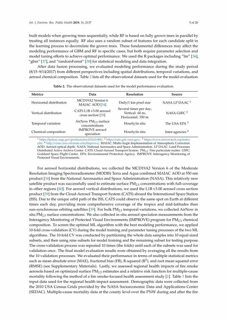
After data fusion processing, we evaluated modeling performance during the study period(8/15–9/14/2017) from different perspectives including spatial distributions, temporal variations, andaerosol chemical composition. Table 2 lists all the observational datasets used for the model evaluation.

Table 2. The observational datasets used for the model performance evaluation.

Metrics Data Resolution Source

Horizontal distribution MCD19A2 Version 6MAIAC AOD [34] Daily/1 km pixel size NASA LP DAAC 1

Vertical distribution CATS L1B v3.00 aerosolcross section [39]

Several times per day;Vertical: 60 m;

Horizontal: 350 mNASA GSFC 2

Temporal variation AirNow PM2.5 surfaceconcentrations Hourly/in situ The USA EPA 3

Chemical composition IMPROVE aerosolspeciation Hourly/in situ Inter-agencies 4

1 https://lpdaac.usgs.gov/products/mcd19a2v006/. 2 https://cats.gsfc.nasa.gov/. 3 https://www.airnowtech.org/index.cfm. 4 http://vista.cira.colostate.edu/Improve/. MAIAC: Multi-Angle Implementation of Atmospheric Correction.AOD: Aerosol optical depth. NASA: National Aeronautics and Space Administration. LP DAAC: Land ProcessesDistributed Active Archive Center. CATS: Cloud-Aerosol Transport System. PM2.5: Fine particulate matter. GSFC:Goddard Space Flight Center. EPA: Environmental Protection Agency. IMPROVE: Interagency Monitoring ofProtected Visual Environments.

For aerosol horizontal distributions, we collected the MCD19A2 Version 6 of the ModerateResolution Imaging Spectroradiometer (MODIS) Terra and Aqua combined MAIAC AOD at 550 nmproduct [34] from the National Aeronautics and Space Administration (NASA). This relatively newsatellite product was successfully used to estimate surface PM2.5 concentrations with full-coveragein other regions [40]. For aerosol vertical distributions, we used the L1B v3.00 aerosol cross sectionproduct [39] from the Cloud-Aerosol Transport System (CATS) aboard the International Space Station(ISS). Due to the unique orbit path of the ISS, CATS could observe the same spot on Earth at differenttimes each day, providing more comprehensive coverage of the tropics and mid-latitudes thansun-synchronous orbiting satellites [39]. For bulk PM2.5 temporal variations, we collected AirNow insitu PM2.5 surface concentrations. We also collected in situ aerosol speciation measurements from theInteragency Monitoring of Protected Visual Environments (IMPROVE) program for PM2.5 chemicalcomposition. To screen the optimal ML algorithm with the best modeling performance, we applied10-fold cross-validation (CV) during the model training and parameter tuning processes of the two MLalgorithms. The 10-fold CV was conducted by partitioning the whole data samples into 10 equal sizedsubsets, and then using nine subsets for model training and the remaining subset for testing purpose.The cross-validation process was repeated 10 times (the folds) until each of the subsets was used forvalidation once. The final model evaluation results were obtained by averaging all the results fromthe 10 validation processes. We evaluated their performance in terms of multiple statistical metricssuch as mean absolute error (MAE), fractional bias (FB), R-squared (R2), and root mean squared error(RMSE) (see Supplementary Materials). Lastly, we assessed regional health impacts of fire smokeaerosols based on optimized surface PM2.5 estimates and a relative risk function for multiple-causemortality following the method of a fire smoke-focused health assessment study [1]. Table 3 lists theinput data used for the regional health impact assessment. Demographic data were collected fromthe 2010 USA Census Grids provided by the NASA Socioeconomic Data and Applications Center(SEDAC). Multiple-cause mortality data at the county level over the PNW during and after the fire

Int. J. Environ. Res. Public Health 2019, 16, 2137 6 of 20

smoke pollution episode were collected from the 2017 multiple cause of death online database byWide-ranging ONline Data for Epidemiologic Research (WONDER) of Centers for Disease Controland Prevention (CDC). The multiple-cause mortality attributable to PM2.5 exposure during the firesmoke pollution episode was estimated using the following exposure-response function adapted fromJohnston et al. [1]:

Mortality attributable to PM2.5 exposure =∑n

PM2.5DPM2.5 ×M× (RRSI(PM2.5) − 1), (2)

where PM2.5 is daily average surface PM2.5 concentrations with minimum and maximum values of5 and 200 µg m−3, respectively. Following Johnston et al. [1], we excluded the grid cells with dailyexposure estimates of less than 5 µg m−3 and fixed grid cells with exposure estimates larger than200 µg m−3 to a maximum threshold of 200 µg m−3. Although there is little evidence for a thresholdPM2.5 mortality function, the minimum threshold was set to reflect the less certainty of the shapeof the exposure-response relationship at low PM2.5 levels [41], while the maximum threshold wasset to represent the flat shape of the exposure-response relationship at high concentration levels [42].DPM2.5 is the number of days with daily PM2.5 at certain levels between each PM2.5 concentrationinterval (i.e., each 1 µg m−3 increment between 5 µg m−3 and 200 µg m−3), n is the total numberof concentration intervals, M is the county-level daily average number of multiple cause of deathsbetween August-December of 2017, and RRSI is a relative risk function for multiple-cause mortalitydue to short-term PM2.5 exposure. We downscaled the county-level multiple cause of deaths (M) tothe model-grid scale according to the high-resolution gridded population density data from the 2010USA Census Grids. Therefore, we were able to estimate population exposure risks with both griddedmortality and PM2.5 concentrations at the same resolution of modeling grids (i.e., 4 km).

Table 3. The demographic data and relative risk function used for health impact assessment.

Data Description Source

Population The USA Census Grids, 2010 [43] NASA SEDAC 1

Mortality Multiple cause of deaths inAugust–December of 2017 CDC WONDER 2

Relative risk function formultiple-cause mortality

0.11% (95% CI: 0, 0.26%) per 1 µgm−3 increase of surface PM2.5

concentrationJohnston et al. [1]

1 http://sedac.ciesin.columbia.edu/data/set/usgrid-summary-file1-2010. 2 https://wonder.cdc.gov/mcd.html. SEDAC:Socioeconomic Data and Applications Center. CDC: Centers for Disease Control and Prevention. WONDER:Wide-ranging ONline Data for Epidemiologic Research.

3. Observational and Modeling Results

3.1. The 2017 PNW Fire Smoke Pollution Episode

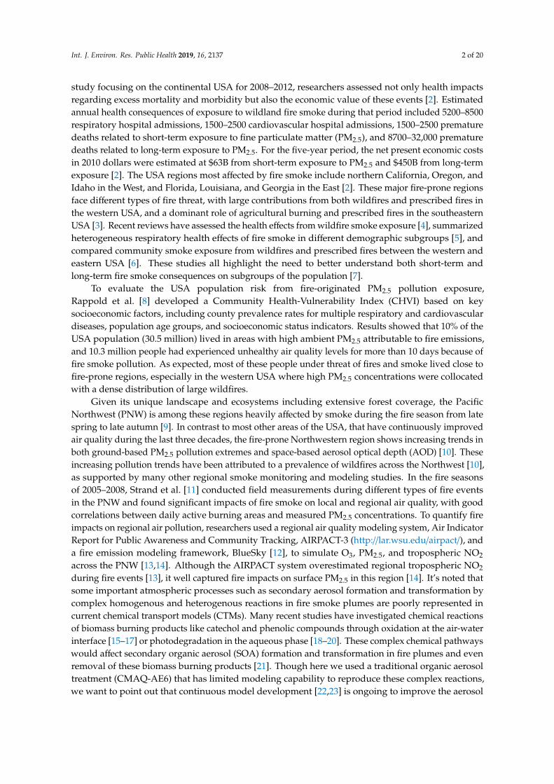
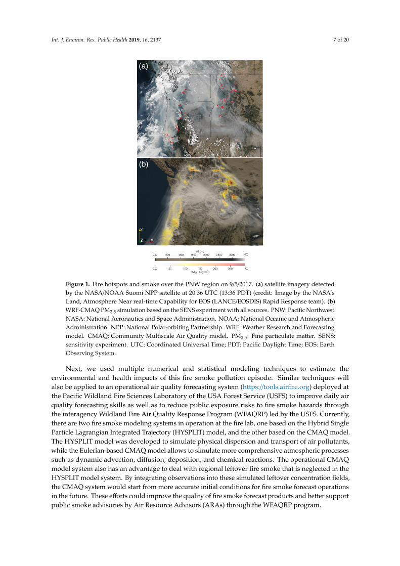
The 2017 fire smoke pollution episode in the PNW was characterized by a series of region-widelarge wildland fires in the eastern and western PNW mountains, as well as heavy fire smoke fromthese fires from mid-August to mid-September 2017. Figure 1 shows fire hotspots and smoke over thePNW on 5 September 2017 in the space-based imagery (Figure 1a) detected by the Suomi NationalPolar-orbiting Partnership (NPP) satellite project (http://www.nasa.gov/NPP), a collaboration betweenNASA, National Oceanic and Atmospheric Administration (NOAA), and Department of Defense,and the model-based PM2.5 simulation (Figure 1b). Major population centers such as the Seattleand Portland metropolitan areas were engulfed by heavy and prolonged smoke during this period.A ground measurement station in Missoula, Montana observed ~500 h heavy smoke episodes, with upto 471 µg m−3 of hourly PM2.5 [44]. Such prolonged exposure to severe smoke pollution may causeserious public health problems in this region.

Int. J. Environ. Res. Public Health 2019, 16, 2137 7 of 20

1

Figure 1. Fire hotspots and smoke over the PNW region on 9/5/2017. (a) satellite imagery detectedby the NASA/NOAA Suomi NPP satellite at 20:36 UTC (13:36 PDT) (credit: Image by the NASA’sLand, Atmosphere Near real-time Capability for EOS (LANCE/EOSDIS) Rapid Response team). (b)WRF-CMAQ PM2.5 simulation based on the SENS experiment with all sources. PNW: Pacific Northwest.NASA: National Aeronautics and Space Administration. NOAA: National Oceanic and AtmosphericAdministration. NPP: National Polar-orbiting Partnership. WRF: Weather Research and Forecastingmodel. CMAQ: Community Multiscale Air Quality model. PM2.5: Fine particulate matter. SENS:sensitivity experiment. UTC: Coordinated Universal Time; PDT: Pacific Daylight Time; EOS: EarthObserving System.

Next, we used multiple numerical and statistical modeling techniques to estimate theenvironmental and health impacts of this fire smoke pollution episode. Similar techniques willalso be applied to an operational air quality forecasting system (https://tools.airfire.org) deployed atthe Pacific Wildland Fire Sciences Laboratory of the USA Forest Service (USFS) to improve daily airquality forecasting skills as well as to reduce public exposure risks to fire smoke hazards throughthe interagency Wildland Fire Air Quality Response Program (WFAQRP) led by the USFS. Currently,there are two fire smoke modeling systems in operation at the fire lab, one based on the Hybrid SingleParticle Lagrangian Integrated Trajectory (HYSPLIT) model, and the other based on the CMAQ model.The HYSPLIT model was developed to simulate physical dispersion and transport of air pollutants,while the Eulerian-based CMAQ model allows to simulate more comprehensive atmospheric processessuch as dynamic advection, diffusion, deposition, and chemical reactions. The operational CMAQmodel system also has an advantage to deal with regional leftover fire smoke that is neglected in theHYSPLIT model system. By integrating observations into these simulated leftover concentration fields,the CMAQ system would start from more accurate initial conditions for fire smoke forecast operationsin the future. These efforts could improve the quality of fire smoke forecast products and better supportpublic smoke advisories by Air Resource Advisors (ARAs) through the WFAQRP program.

Int. J. Environ. Res. Public Health 2019, 16, 2137 8 of 20

3.2. Model Simulation and Evalution Results

3.2.1. Gap-Filling for MAIAC AOD

We first compared the WRF-CMAQ model-simulated AOD from the SENS experiment with theMAIAC satellite retrievals in terms of fire smoke horizontal distributions. More than half of the PNWis covered by missing values of the MAIAC AOD on 7 September 2017 (Figure 2a); these missingvalues may be related to regional cloud contamination, mountainous terrain, and high surface albedoissues in the satellite retrieval algorithm [45]. Such missing value problems also exist on other daysof the study period and require gap-filling for further application in estimation of surface PM2.5.To solve this problem, we implemented ML-based gap-filling processing for missing values in theraw MAIAC AOD products based on WRF-CMAQ simulated AOD and meteorological variables.Although the model simulated AOD are low-biased in general (Figure 2b), they still captured theregional distributions of fire aerosols before and after gap-filling processing with different ML-basedalgorithms (Figure 2c,d). Both GBM (r = 0.96) and RF (r = 0.96) methods show greatly improved spatialcorrelations of gap-filled AOD with satellite retrievals, which increased our confidence of using thesetechniques in the next step to optimize surface PM2.5 concentrations and fire smoke exposures. Wealso compared the statistical performance in terms of spatial correlation (r) and RMSE values for allmodeling days (08/15/2017–09/14/2017) (Supplementary Materials Figure S1).Int. J. Environ. Res. Public Health 2019, 16, x 9 of 22

Figure 2. Comparison of the MAIAC AOD at 550 nm and model simulated AOD results at 20:15 UTC (13:15 PDT) on 9/7/2017. (a) the MAIAC AOD product onboard the MODIS Aqua satellite; (b) CMAQ simulated AOD; (c) bias-adjusted AOD by the RF method; (d) same as (c) but by the GBM method. The r-values on top-left corners of the subplots (b)–(d) denote spatial correlation coefficients between each model result and corresponding MAIAC AOD product. MAIAC: Multi-Angle Implementation of Atmospheric Correction. AOD: aerosol optical depth. MODIS: Moderate Resolution Imaging Spectroradiometer. CMAQ: Community Multiscale Air Quality model. RF: Random forest. GBM: Generalized boosting model.

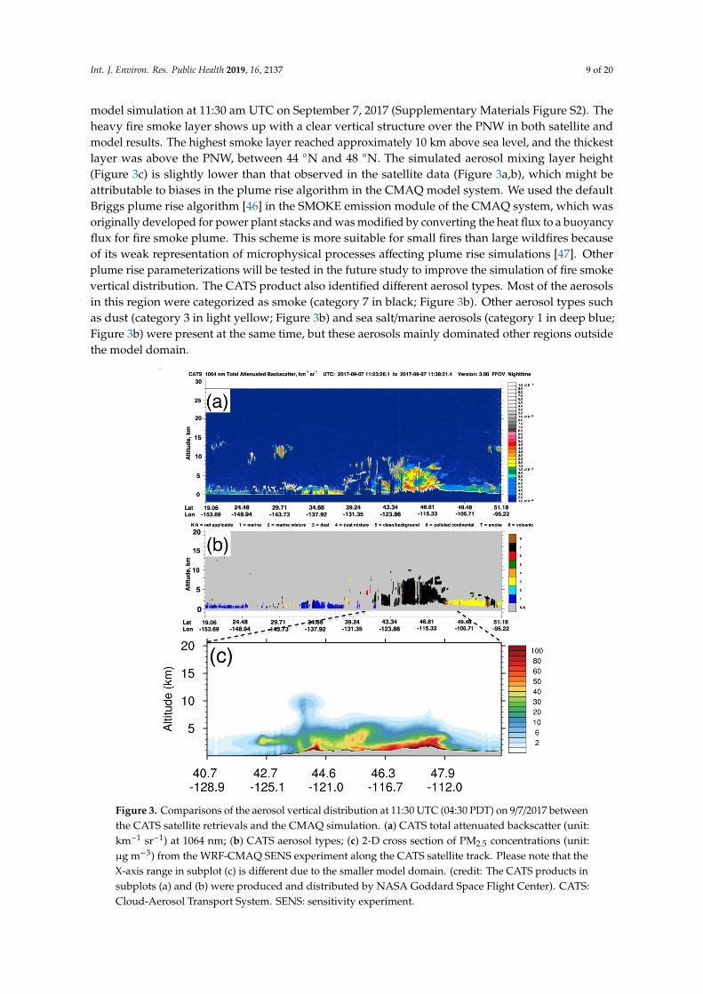
Besides horizontal distributions, we also evaluated smoke vertical distributions. Figure 3 shows comparisons of space-based aerosol cross sections retrieved by the CATS system and the WRF-CMAQ model simulation at 11:30 am UTC on September 7, 2017 (Supplementary Materials Figure S2). The heavy fire smoke layer shows up with a clear vertical structure over the PNW in both satellite and model results. The highest smoke layer reached approximately 10 km above sea level, and the thickest layer was above the PNW, between 44 °N and 48 °N. The simulated aerosol mixing layer height (Figure 3c) is slightly lower than that observed in the satellite data (Figure 3a, b), which might be attributable to biases in the plume rise algorithm in the CMAQ model system. We used the default Briggs plume rise algorithm [46] in the SMOKE emission module of the CMAQ system, which was originally developed for power plant stacks and was modified by converting the heat flux to a buoyancy flux for fire smoke plume. This scheme is more suitable for small fires than large wildfires because of its weak representation of microphysical processes affecting plume rise simulations [47]. Other plume rise parameterizations will be tested in the future study to improve the simulation of fire smoke vertical distribution. The CATS product also identified different aerosol types. Most of the aerosols in this region were categorized as smoke (category 7 in black; Figure 3b). Other aerosol types such as dust (category 3 in light yellow; Figure 3b) and sea salt/marine aerosols

Figure 2. Comparison of the MAIAC AOD at 550 nm and model simulated AOD results at 20:15 UTC(13:15 PDT) on 9/7/2017. (a) the MAIAC AOD product onboard the MODIS Aqua satellite; (b) CMAQsimulated AOD; (c) bias-adjusted AOD by the RF method; (d) same as (c) but by the GBM method.The r-values on top-left corners of the subplots (b)–(d) denote spatial correlation coefficients betweeneach model result and corresponding MAIAC AOD product. MAIAC: Multi-Angle Implementationof Atmospheric Correction. AOD: aerosol optical depth. MODIS: Moderate Resolution ImagingSpectroradiometer. CMAQ: Community Multiscale Air Quality model. RF: Random forest. GBM:Generalized boosting model.

Besides horizontal distributions, we also evaluated smoke vertical distributions. Figure 3 showscomparisons of space-based aerosol cross sections retrieved by the CATS system and the WRF-CMAQ

Int. J. Environ. Res. Public Health 2019, 16, 2137 9 of 20

model simulation at 11:30 am UTC on September 7, 2017 (Supplementary Materials Figure S2). Theheavy fire smoke layer shows up with a clear vertical structure over the PNW in both satellite andmodel results. The highest smoke layer reached approximately 10 km above sea level, and the thickestlayer was above the PNW, between 44 ◦N and 48 ◦N. The simulated aerosol mixing layer height(Figure 3c) is slightly lower than that observed in the satellite data (Figure 3a,b), which might beattributable to biases in the plume rise algorithm in the CMAQ model system. We used the defaultBriggs plume rise algorithm [46] in the SMOKE emission module of the CMAQ system, which wasoriginally developed for power plant stacks and was modified by converting the heat flux to a buoyancyflux for fire smoke plume. This scheme is more suitable for small fires than large wildfires becauseof its weak representation of microphysical processes affecting plume rise simulations [47]. Otherplume rise parameterizations will be tested in the future study to improve the simulation of fire smokevertical distribution. The CATS product also identified different aerosol types. Most of the aerosolsin this region were categorized as smoke (category 7 in black; Figure 3b). Other aerosol types suchas dust (category 3 in light yellow; Figure 3b) and sea salt/marine aerosols (category 1 in deep blue;Figure 3b) were present at the same time, but these aerosols mainly dominated other regions outsidethe model domain.

Int. J. Environ. Res. Public Health 2019, 16, x 10 of 22

(category 1 in deep blue; Figure 3b) were present at the same time, but these aerosols mainly dominated other regions outside the model domain.

Figure 3. Comparisons of the aerosol vertical distribution at 11:30 UTC (04:30 PDT) on 9/7/2017 between the CATS satellite retrievals and the CMAQ simulation. (a) CATS total attenuated backscatter (unit: km−1 sr−1) at 1064 nm; (b) CATS aerosol types; (c) 2-D cross section of PM2.5 concentrations (unit: μg m−3) from the WRF-CMAQ SENS experiment along the CATS satellite track. Please note that the X-axis range in subplot (c) is different due to the smaller model domain. (credit: The CATS products in subplots (a) and (b) were produced and distributed by NASA Goddard Space Flight Center). CATS: Cloud-Aerosol Transport System. SENS: sensitivity experiment.

3.2.2. Data Fusion for Surface PM2.5 Concentrations

After gap filling for missing values in MAIAC AOD, we applied the same data fusion algorithms to optimize surface PM2.5 and smoke exposure estimates based on AirNow in situ observations and WRF-CMAQ model simulations, gap-filled AOD, and reanalysis-based meteorological variables as introduced

Figure 3. Comparisons of the aerosol vertical distribution at 11:30 UTC (04:30 PDT) on 9/7/2017 betweenthe CATS satellite retrievals and the CMAQ simulation. (a) CATS total attenuated backscatter (unit:km−1 sr−1) at 1064 nm; (b) CATS aerosol types; (c) 2-D cross section of PM2.5 concentrations (unit:µg m−3) from the WRF-CMAQ SENS experiment along the CATS satellite track. Please note that theX-axis range in subplot (c) is different due to the smaller model domain. (credit: The CATS products insubplots (a) and (b) were produced and distributed by NASA Goddard Space Flight Center). CATS:Cloud-Aerosol Transport System. SENS: sensitivity experiment.

Int. J. Environ. Res. Public Health 2019, 16, 2137 10 of 20

3.2.2. Data Fusion for Surface PM2.5 Concentrations

After gap filling for missing values in MAIAC AOD, we applied the same data fusion algorithmsto optimize surface PM2.5 and smoke exposure estimates based on AirNow in situ observationsand WRF-CMAQ model simulations, gap-filled AOD, and reanalysis-based meteorological variablesas introduced in Section 2. Figure 4 shows the regional PM2.5 simulation performance of the rawWRF-CMAQ SENS system, which incorporated emission contributions from all major source sectorsincluding both fire and non-fire emissions.

Int. J. Environ. Res. Public Health 2019, 16, x 11 of 22

in Section 2. Figure 4 shows the regional PM2.5 simulation performance of the raw WRF-CMAQ SENS system, which incorporated emission contributions from all major source sectors including both fire and non-fire emissions.

Figure 4. Statistical evaluation results of the raw WRF-CMAQ SENS simulated PM2.5 surface concentrations during 8/15–9/14/2017: (a) monthly averaged PM2.5 surface concentrations (unit: μg m−3). The black circles and red numbers denote 16 selected ground sites for the time series evaluation in Figure 5; (b) temporal correlations (unitless) between the SENS simulation and AirNow observations at each ground site; (c) fractional biases (unit: 100%) based on the SENS simulation and AirNow observations; (d) RMSE (unit: μg m−3) based on the SENS simulation and AirNow observations. RMSE: root mean squared error.

The monthly averaged surface PM2.5 concentration field shows major hotspots in these mountain forests on both sides of the PNW, especially along the Western Cascades and the Bitterroot Range, which are consistent with the satellite imagery in Figure 1. These fire hotspots released large amounts of aerosols and tracer gases in forms of heavy smoke that enveloped almost the whole PNW (Figure 4a). Although the model results show good agreement, with high temporal correlations with AirNow ground monitoring data at most sites (Figure 4b), the negative biases in simulated PM2.5 surface concentrations are pervasive over the whole model domain (Figure 4c). Such underestimation in surface PM2.5 simulation may suggest systematic low bias in primary emission inventories and/or insufficient secondary aerosol formation in simulated fire plumes, both of which require further investigation and correction by pre- and post-processing measures. The site-specific RMSE results (Figure 4d) show a similar pattern with the regional PM2.5 concentrations (Figure 4a), manifesting high values in near-source mountain regions and low values in downstream regions after fire smoke transport and dispersion. This pattern can be explained by the calculation method of RMSE (see Supplementary Materials), which is based on the absolute values of PM2.5 concentrations. Because of the large uncertainty in fire emission inventory, these PM2.5 concentrations that are heavily dominated by fire smoke in near-source regions may suffer a larger influence from bias in estimation of fire emission, contributing to larger RMSE values at near-source sites (Figure 4d).

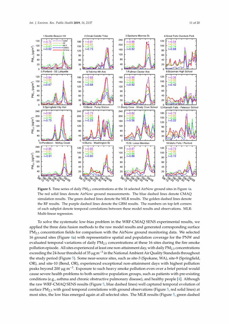
To solve the systematic low-bias problem in the WRF-CMAQ SENS experimental results, we applied the three data fusion methods to the raw model results and generated corresponding surface PM2.5 concentration fields for comparison with the AirNow ground monitoring data. We selected 16 ground sites (Figure 4a) with representative spatial and population coverage for the PNW and evaluated temporal variations of daily PM2.5 concentrations at these 16 sites during the fire smoke pollution episode. All sites

Figure 4. Statistical evaluation results of the raw WRF-CMAQ SENS simulated PM2.5 surfaceconcentrations during 8/15–9/14/2017: (a) monthly averaged PM2.5 surface concentrations (unit:µg m−3). The black circles and red numbers denote 16 selected ground sites for the time seriesevaluation in Figure 5; (b) temporal correlations (unitless) between the SENS simulation and AirNowobservations at each ground site; (c) fractional biases (unit: 100%) based on the SENS simulationand AirNow observations; (d) RMSE (unit: µg m−3) based on the SENS simulation and AirNowobservations. RMSE: root mean squared error.

The monthly averaged surface PM2.5 concentration field shows major hotspots in these mountainforests on both sides of the PNW, especially along the Western Cascades and the Bitterroot Range,which are consistent with the satellite imagery in Figure 1. These fire hotspots released large amountsof aerosols and tracer gases in forms of heavy smoke that enveloped almost the whole PNW (Figure 4a).Although the model results show good agreement, with high temporal correlations with AirNowground monitoring data at most sites (Figure 4b), the negative biases in simulated PM2.5 surfaceconcentrations are pervasive over the whole model domain (Figure 4c). Such underestimation insurface PM2.5 simulation may suggest systematic low bias in primary emission inventories and/orinsufficient secondary aerosol formation in simulated fire plumes, both of which require furtherinvestigation and correction by pre- and post-processing measures. The site-specific RMSE results(Figure 4d) show a similar pattern with the regional PM2.5 concentrations (Figure 4a), manifestinghigh values in near-source mountain regions and low values in downstream regions after fire smoketransport and dispersion. This pattern can be explained by the calculation method of RMSE (seeSupplementary Materials), which is based on the absolute values of PM2.5 concentrations. Because ofthe large uncertainty in fire emission inventory, these PM2.5 concentrations that are heavily dominatedby fire smoke in near-source regions may suffer a larger influence from bias in estimation of fireemission, contributing to larger RMSE values at near-source sites (Figure 4d).

Int. J. Environ. Res. Public Health 2019, 16, 2137 11 of 20

Int. J. Environ. Res. Public Health 2019, 16, x 12 of 22

experienced at least one non-attainment day, with daily PM2.5 concentrations exceeding the 24-hour threshold of 35 μg m−3 in the National Ambient Air Quality Standards throughout the study period (Figure 5). Some near-source sites, such as site-3 (Spokane, WA), site-9 (Springfield, OR), and site-10 (Bend, OR), experienced exceptional non-attainment days with highest pollution peaks beyond 200 μg m−3. Exposure to such heavy smoke pollution even over a brief period would cause severe health problems to both sensitive population groups, such as patients with pre-existing conditions (e.g., asthma and chronic obstructive pulmonary disease), and healthy people [4]. Although the raw WRF-CMAQ SENS results (Figure 5, blue dashed lines) well captured temporal evolution of surface PM2.5 with good temporal correlations with ground observations (Figure 5, red solid lines) at most sites, the low bias emerged again at all selected sites. The MLR results (Figure 5, green dashed lines) somewhat alleviated the low-bias problem but failed to increase temporal correlations for most sites. In comparison, the RF (Figure 5, golden dashed lines) and the GBM (Figure 5, purple dashed lines) methods greatly improved both the accuracy and correlation of modeling results at most ground sites. The RF method outperformed the GBM method, in slightly better agreement with observations.

Figure 5. Time series of daily PM2.5 concentrations at the 16 selected AirNow ground sites in Figure 4a. The red solid lines denote AirNow ground measurements. The blue dashed lines denote CMAQ simulation results. The green dashed lines denote the MLR results. The golden dashed lines denote the RF results. The

Figure 5. Time series of daily PM2.5 concentrations at the 16 selected AirNow ground sites in Figure 4a.The red solid lines denote AirNow ground measurements. The blue dashed lines denote CMAQsimulation results. The green dashed lines denote the MLR results. The golden dashed lines denotethe RF results. The purple dashed lines denote the GBM results. The numbers on top-left cornersof each subplot denote temporal correlations between these model results and observations. MLR:Multi-linear regression.

To solve the systematic low-bias problem in the WRF-CMAQ SENS experimental results, weapplied the three data fusion methods to the raw model results and generated corresponding surfacePM2.5 concentration fields for comparison with the AirNow ground monitoring data. We selected16 ground sites (Figure 4a) with representative spatial and population coverage for the PNW andevaluated temporal variations of daily PM2.5 concentrations at these 16 sites during the fire smokepollution episode. All sites experienced at least one non-attainment day, with daily PM2.5 concentrationsexceeding the 24-hour threshold of 35µg m−3 in the National Ambient Air Quality Standards throughoutthe study period (Figure 5). Some near-source sites, such as site-3 (Spokane, WA), site-9 (Springfield,OR), and site-10 (Bend, OR), experienced exceptional non-attainment days with highest pollutionpeaks beyond 200 µg m−3. Exposure to such heavy smoke pollution even over a brief period wouldcause severe health problems to both sensitive population groups, such as patients with pre-existingconditions (e.g., asthma and chronic obstructive pulmonary disease), and healthy people [4]. Althoughthe raw WRF-CMAQ SENS results (Figure 5, blue dashed lines) well captured temporal evolution ofsurface PM2.5 with good temporal correlations with ground observations (Figure 5, red solid lines) atmost sites, the low bias emerged again at all selected sites. The MLR results (Figure 5, green dashed

Int. J. Environ. Res. Public Health 2019, 16, 2137 12 of 20

lines) somewhat alleviated the low-bias problem but failed to increase temporal correlations for mostsites. In comparison, the RF (Figure 5, golden dashed lines) and the GBM (Figure 5, purple dashedlines) methods greatly improved both the accuracy and correlation of modeling results at most groundsites. The RF method outperformed the GBM method, in slightly better agreement with observations.

The scatter plots in Figure 6 give a better presentation of comparisons between the daily modelingresults and the AirNow in situ observations. As discussed above, the raw CMAQ SENS results withoutdata integration show upward shifted distributions, with the data centroid above the 1:1 referenceline (Figure 6a), suggesting low bias in the raw modeling results (Table 4). After model parametertuning (Supplementary Materials Figures S3 and S4), all three data fusion algorithms improved thedata distributions to different extent, with the best performance in the RF results in most statisticalmetrics (Figure 6c, Table 4). The regionally averaged PM2.5 concentration increased significantly afterdata integration, especially weighted by population density. The area-weighted regional average PM2.5

concentration increased by 90% in the ensemble mean of the three data fusion algorithms (MLR, RF,and GBM), and the population-weighted regional average PM2.5 concentration increased by 193% inthe ensemble mean. Since the health impact assessment was based on population exposure to PM2.5

pollution, we mainly focus on the RF result that shows the best modeling performance of surfacePM2.5 concentrations.

Int. J. Environ. Res. Public Health 2019, 16, x 13 of 22

purple dashed lines denote the GBM results. The numbers on top-left corners of each subplot denote temporal correlations between these model results and observations. MLR: Multi-linear regression. The scatter plots in Figure 6 give a better presentation of comparisons between the daily modeling results

and the AirNow in situ observations. As discussed above, the raw CMAQ SENS results without data integration show upward shifted distributions, with the data centroid above the 1:1 reference line (Figure 6a), suggesting low bias in the raw modeling results (Table 4). After model parameter tuning (Supplementary Materials Figures S3 and S4), all three data fusion algorithms improved the data distributions to different extent, with the best performance in the RF results in most statistical metrics (Figure 6c, Table 4). The regionally averaged PM2.5 concentration increased significantly after data integration, especially weighted by population density. The area-weighted regional average PM2.5 concentration increased by 90% in the ensemble mean of the three data fusion algorithms (MLR, RF, and GBM), and the population-weighted regional average PM2.5 concentration increased by 193% in the ensemble mean. Since the health impact assessment was based on population exposure to PM2.5 pollution, we mainly focus on the RF result that shows the best modeling performance of surface PM2.5 concentrations.

Figure 6. Comparisons of daily PM2.5 model simulation before and after data integration with AirNow ground observations during the fire smoke pollution episode. (a) a scatter plot of PM2.5 concentrations on a log scale based on the raw WRF-CMAQ SENS simulation and AirNow observations; (b) same as (a) but based on the MLR data integration method; (c) same as (a) but based on the RF method; (d) same as (a) but based on the GBM method. The color shading in all subplots denotes the PM2.5 data density in terms of sample counts.

Figure 6. Comparisons of daily PM2.5 model simulation before and after data integration with AirNowground observations during the fire smoke pollution episode. (a) a scatter plot of PM2.5 concentrationson a log scale based on the raw WRF-CMAQ SENS simulation and AirNow observations; (b) same as(a) but based on the MLR data integration method; (c) same as (a) but based on the RF method; (d)same as (a) but based on the GBM method. The color shading in all subplots denotes the PM2.5 datadensity in terms of sample counts.

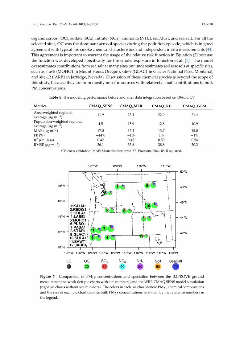
Before assessing regional health impacts with the surface PM2.5 exposure estimates, we evaluatedPM2.5 chemical composition by comparing model-simulated aerosol species (the SENS results) withthe in situ measurements from the IMPROVE network over the PNW region. Figure 7 shows thecomparison results of seven chemical species at 12 IMPROVE sites. The pie sizes denote bulk PM2.5

concentrations and colored fractions denote the chemical composition, such as elemental carbon (EC),

Int. J. Environ. Res. Public Health 2019, 16, 2137 13 of 20

organic carbon (OC), sulfate (SO4), nitrate (NO3), ammonia (NH4), soil/dust, and sea salt. For all theselected sites, OC was the dominant aerosol species during the pollution episode, which is in goodagreement with typical fire smoke chemical characteristics and independent in situ measurements [44].This agreement is important to warrant the usage of the relative risk function in Equation (2) becausethe function was developed specifically for fire smoke exposure in Johnston et al. [1]. The modeloverestimates contributions from sea salt at many sites but underestimates soil aerosols at specific sites,such as site-5 (MOHO1 in Mount Hood, Oregon), site-9 (GLAC1 in Glacier National Park, Montana),and site-12 (JARB1 in Jarbidge, Nevada). Discussion of these chemical species is beyond the scope ofthis study, because they are from mostly non-fire sources with relatively small contributions to bulkPM concentrations.

Table 4. The modeling performance before and after data integration based on 10-fold CV.

Metrics CMAQ_SENS CMAQ_MLR CMAQ_RF CMAQ_GBM

Area-weighted regionalaverage (µg m−3) 11.9 23.4 22.9 21.4

Population-weighted regionalaverage (µg m−3) 4.5 15.9 12.8 10.9

MAE (µg m−3) 17.0 17.4 13.7 15.0FB (%) −44% −1% 1% −1%R2 (unitless) 0.42 0.45 0.59 0.54RMSE (µg m−3) 36.1 33.8 28.8 30.3

CV: cross-validation. MAE: Mean absolute error. FB: Fractional bias, R2: R-squared.

Int. J. Environ. Res. Public Health 2019, 16, x 14 of 22

Table 4. The modeling performance before and after data integration based on 10-fold CV.

Metrics CMAQ_SENS CMAQ_MLR CMAQ_RF CMAQ_GBM Area-weighted regional average (μg m−3) 11.9 23.4 22.9 21.4 Population-weighted regional average (μg m−3) 4.5 15.9 12.8 10.9 MAE (μg m−3) 17.0 17.4 13.7 15.0 FB (%) −44% −1% 1% −1% R2 (unitless) 0.42 0.45 0.59 0.54 RMSE (μg m−3) 36.1 33.8 28.8 30.3

CV: cross-validation. MAE: Mean absolute error. FB: Fractional bias, R2: R-squared.

Before assessing regional health impacts with the surface PM2.5 exposure estimates, we evaluated PM2.5 chemical composition by comparing model-simulated aerosol species (the SENS results) with the in situ measurements from the IMPROVE network over the PNW region. Figure 7 shows the comparison results of seven chemical species at 12 IMPROVE sites. The pie sizes denote bulk PM2.5 concentrations and colored fractions denote the chemical composition, such as elemental carbon (EC), organic carbon (OC), sulfate (SO4), nitrate (NO3), ammonia (NH4), soil/dust, and sea salt. For all the selected sites, OC was the dominant aerosol species during the pollution episode, which is in good agreement with typical fire smoke chemical characteristics and independent in situ measurements [44]. This agreement is important to warrant the usage of the relative risk function in Equation (2) because the function was developed specifically for fire smoke exposure in Johnston et al. [1]. The model overestimates contributions from sea salt at many sites but underestimates soil aerosols at specific sites, such as site-5 (MOHO1 in Mount Hood, Oregon), site-9 (GLAC1 in Glacier National Park, Montana), and site-12 (JARB1 in Jarbidge, Nevada). Discussion of these chemical species is beyond the scope of this study, because they are from mostly non-fire sources with relatively small contributions to bulk PM concentrations.

Figure 7. Comparison of PM2.5 concentrations and speciation between the IMPROVE ground measurement network (left pie charts with site numbers) and the WRF-CMAQ SENS model simulation (right pie charts

Figure 7. Comparison of PM2.5 concentrations and speciation between the IMPROVE groundmeasurement network (left pie charts with site numbers) and the WRF-CMAQ SENS model simulation(right pie charts without site numbers). The colors in each pie chart denote PM2.5 chemical compositionsand the size of each pie chart denotes bulk PM2.5 concentrations as shown by the reference numbers inthe legend.

Int. J. Environ. Res. Public Health 2019, 16, 2137 14 of 20

3.3. Regional Health Impact Assessment

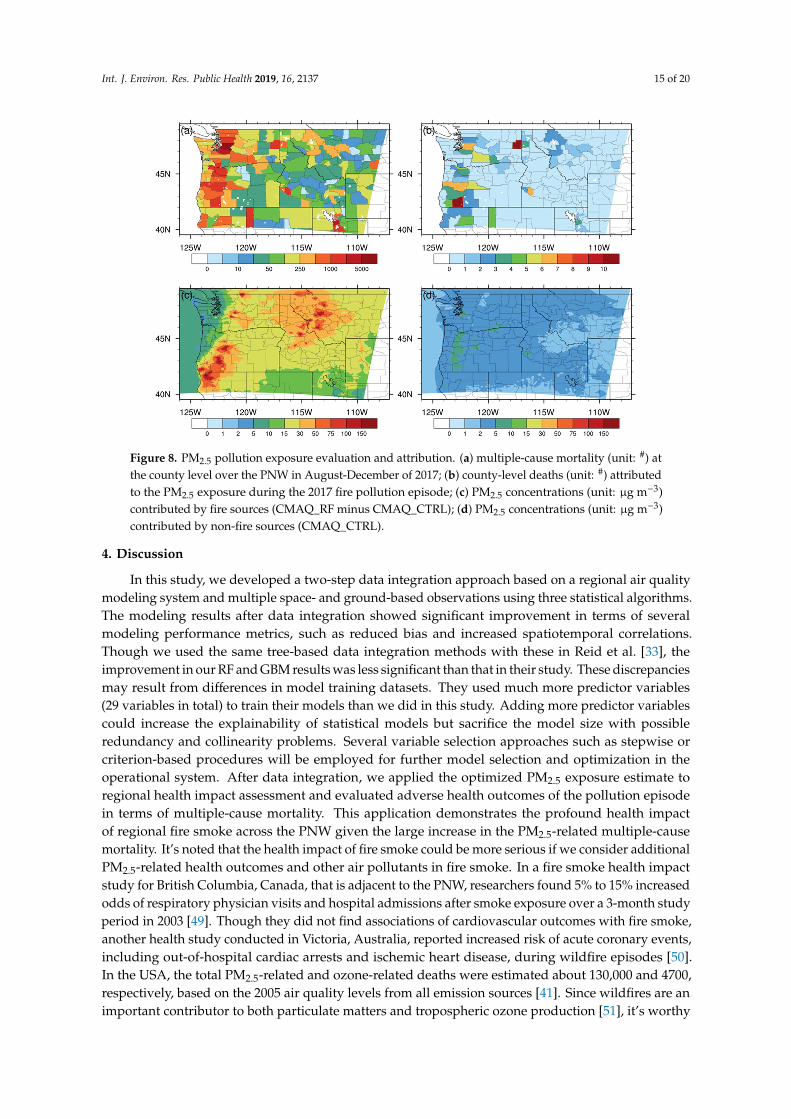
Lastly, we conducted regional health impact assessment for the 2017 PNW fire smoke pollutionepisode following Johnston et al.’s method [1]. Figure 8a shows regional multiple-cause mortality atthe county level over the PNW in August-December of 2017, and Figure 8b shows county-level deathsattributed to the PM2.5 pollution exposure based on the RF results. These regions that were heavilyaffected by PM2.5 pollution are consistent with the spatial distribution of major population centersover the PNW, which also have relatively large numbers of deaths. However, the mountain regions ofthe Western Cascades and the Bitterroot Range showed more significant health outcomes because ofheavier fire smoke exposure in these two near-source areas than in the Puget Sound region, despitethe much larger urban population and mortality. Fire smoke mostly blanketed the southwestern andnortheastern corners of the PNW, with gradually decreasing PM2.5 concentrations from near-sourceregions to downwind regions (Figure 8c). Fire smoke severely undermined public health, with mostfire smoke-related deaths occurring in Spokane County (12; 95% CI: 0, 28) of eastern Washington andJackson County (11; 95% CI: 0, 26) of southwestern Oregon. Some distant downstream regions suchas Salt Lake County (4; 95% CI: 0, 9) in Utah also witnessed moderate health effects of fire smoke.The population-weighted regional mean PM2.5 concentration based on the RF results is 13 µg m−3

(Table 4), to which fire sources contributed around 85% (11 µg m−3; Figure 8c) and non-fire sourcescontributed only 15% (2 µg m−3; Figure 8d). Though PM2.5 concentrations in the CMAQ_CTRLexperiment (Figure 8d) were not corrected by observations, it’s noted that this estimate of the regionalbackground PM2.5 concentration for the PNW is similar with a previous model-based study (2 µg m−3

averaged from 18 rural sites and 4 µg m−3 averaged from 36 urban/suburban sites with non-fire sourcesin the PNW) [14] and an observation-based study (3.3 µg m−3 averaged from seven backgroundmonitoring sites during non-fire season in the PNW) [48]. We also compared the time averagedCMAQ_CTRL results with the AirNow ground observations during a non-fire period (June–July,2017) before the fire smoke episode (Supplementary Materials Figure S5). The comparison showedgood agreement on a regional scale, suggesting the effective representativeness of the uncorrectedCMAQ_CTRL results for non-fire sources. Based on the RF method, the estimated total number ofregional deaths attributable to the 30-day PM2.5 exposure was 183 (95% CI: 0, 432), and fire smoke wasthe largest PM2.5 pollution source. This estimate varies little if we change the data integration methodto the other algorithms. The uncertainty range is ~10% among the three data integration methods,with a similar estimate based on the GBM results (182; 95% CI: 0, 431) and a higher estimate based onthe MLR results (202; 95% CI: 0, 477). The total PM2.5 attributable regional deaths would decreasesignificantly to 9 (5% CI: 0, 20) if without the fire events in the CTRL experiment, suggesting evenlarger contributions (95%) of fire emissions to regional health effects due to the piecewise feature in theexposure-response function (Equation (2)).

Int. J. Environ. Res. Public Health 2019, 16, 2137 15 of 20Int. J. Environ. Res. Public Health 2019, 16, x 16 of 22

Figure 8. PM2.5 pollution exposure evaluation and attribution. (a) multiple-cause mortality (unit: #) at the county level over the PNW in August-December of 2017; (b) county-level deaths (unit: #) attributed to the PM2.5 exposure during the 2017 fire pollution episode; (c) PM2.5 concentrations (unit: μg m−3) contributed by fire sources (CMAQ_RF minus CMAQ_CTRL); (d) PM2.5 concentrations (unit: μg m−3) contributed by non-fire sources (CMAQ_CTRL).

4. Discussion

In this study, we developed a two-step data integration approach based on a regional air quality modeling system and multiple space- and ground-based observations using three statistical algorithms. The modeling results after data integration showed significant improvement in terms of several modeling performance metrics, such as reduced bias and increased spatiotemporal correlations. Though we used the same tree-based data integration methods with these in Reid et al. [33], the improvement in our RF and GBM results was less significant than that in their study. These discrepancies may result from differences in model training datasets. They used much more predictor variables (29 variables in total) to train their models than we did in this study. Adding more predictor variables could increase the explainability of statistical models but sacrifice the model size with possible redundancy and collinearity problems. Several variable selection approaches such as stepwise or criterion-based procedures will be employed for further model selection and optimization in the operational system. After data integration, we applied the optimized PM2.5 exposure estimate to regional health impact assessment and evaluated adverse health outcomes of the pollution episode in terms of multiple-cause mortality. This application demonstrates the profound health impact of regional fire smoke across the PNW given the large increase in the PM2.5-related multiple-cause mortality. It’s noted that the health impact of fire smoke could be more serious if we consider additional PM2.5-related health outcomes and other air pollutants in fire smoke. In a fire smoke health impact study for British Columbia, Canada, that is adjacent to the PNW, researchers found 5% to 15% increased odds of respiratory physician visits and hospital admissions after smoke exposure over a 3-month study period in 2003 [49]. Though they did not find associations of cardiovascular outcomes with fire smoke, another health study conducted in Victoria, Australia, reported increased risk of acute coronary events, including out-of-hospital cardiac arrests and ischemic heart disease, during wildfire episodes [50].

Figure 8. PM2.5 pollution exposure evaluation and attribution. (a) multiple-cause mortality (unit: #) atthe county level over the PNW in August-December of 2017; (b) county-level deaths (unit: #) attributedto the PM2.5 exposure during the 2017 fire pollution episode; (c) PM2.5 concentrations (unit: µg m−3)contributed by fire sources (CMAQ_RF minus CMAQ_CTRL); (d) PM2.5 concentrations (unit: µg m−3)contributed by non-fire sources (CMAQ_CTRL).

4. Discussion

In this study, we developed a two-step data integration approach based on a regional air qualitymodeling system and multiple space- and ground-based observations using three statistical algorithms.The modeling results after data integration showed significant improvement in terms of severalmodeling performance metrics, such as reduced bias and increased spatiotemporal correlations.Though we used the same tree-based data integration methods with these in Reid et al. [33], theimprovement in our RF and GBM results was less significant than that in their study. These discrepanciesmay result from differences in model training datasets. They used much more predictor variables(29 variables in total) to train their models than we did in this study. Adding more predictor variablescould increase the explainability of statistical models but sacrifice the model size with possibleredundancy and collinearity problems. Several variable selection approaches such as stepwise orcriterion-based procedures will be employed for further model selection and optimization in theoperational system. After data integration, we applied the optimized PM2.5 exposure estimate toregional health impact assessment and evaluated adverse health outcomes of the pollution episodein terms of multiple-cause mortality. This application demonstrates the profound health impactof regional fire smoke across the PNW given the large increase in the PM2.5-related multiple-causemortality. It’s noted that the health impact of fire smoke could be more serious if we consider additionalPM2.5-related health outcomes and other air pollutants in fire smoke. In a fire smoke health impactstudy for British Columbia, Canada, that is adjacent to the PNW, researchers found 5% to 15% increasedodds of respiratory physician visits and hospital admissions after smoke exposure over a 3-month studyperiod in 2003 [49]. Though they did not find associations of cardiovascular outcomes with fire smoke,another health study conducted in Victoria, Australia, reported increased risk of acute coronary events,including out-of-hospital cardiac arrests and ischemic heart disease, during wildfire episodes [50].In the USA, the total PM2.5-related and ozone-related deaths were estimated about 130,000 and 4700,respectively, based on the 2005 air quality levels from all emission sources [41]. Since wildfires are animportant contributor to both particulate matters and tropospheric ozone production [51], it’s worthy

Int. J. Environ. Res. Public Health 2019, 16, 2137 16 of 20

to expand the research scope to include both PM2.5-related and ozone-related health effects duringfire events.

This study also highlights great potential of the ML-based data integration approach for not onlyhealth impact assessments of fire smoke exposure, but also operational air quality forecasting andreanalysis operations for early warning of fire smoke hazards. Previous studies suggested improvedpublic health preparedness with integrated fire smoke forecast products [52] and huge economicbenefit of forest-based interventions by reducing the health and economic burden of wildfires [53]. Theinteragency WFAQRP program led by the USFS would provide an effective working mechanism toachieve this goal with broad socioeconomic benefit for the USA. The nationwide deployment of ARAssupported by this program has been increasing throughout the past few years. These ARAs serve as abridge between timely fire smoke information and the vulnerable population in fire-prone regions.With effective interventions through strengthened self and group protection, the adverse health effectsand economic burden of fire smoke could be largely reduced.

To advance the research progress in related fields, we suggest three areas that deserve attention infuture research. Firstly, continuous improvement of operational fire smoke forecasting and reanalysissystems and products at both regional and national scales is needed for long-term health impactassessments of fire smoke in the USA and elsewhere. This improvement would be enhanced from (a)application of newly available satellite observations, such as those from geostationary GOES-16/17satellites with much higher temporal resolution, (b) advanced data-driven deep learning algorithms(e.g., Deep Convolution Neural Network), and (c) further development of fully coupled fire modelswith consideration of dynamic fire-atmosphere interactions across scales (e.g., WRF-SFIRE [54] andWRF-Fire [55]) as well as more comprehensive modeling capability of homogenous and heterogenousreactions for fire smoke aerosols. At global scales, one could apply continuously updating satellite-basedglobal fire emission products [56] and newly developed process-based fire models [57] embeddedin state-of-the-science earth system models for retrospective/predictive health and socioeconomicassessment of broad fire impacts.

Besides the spatial and temporal expansion of this integrated approach, we also emphasize theimportance of aerosol chemical composition and its influence on short-term and long-term healtheffects in different population subgroups. Previous studies have reviewed aerosol composition-specifichealth effects based on oxidative stress and aerosol toxicity from different emission sources and burningphases [58,59]. Changes in aerosol speciation would result in distinctly different health outcomesregarding respiratory and cardiovascular diseases, morbidity, and mortality, highlighting the need forsource-specific health impact assessment studies in the future.

Lastly, reduced uncertainties in exposure-response functions are also expected by advancingcohort-based health studies regarding fire smoke exposure and health effects. Currently, largeuncertainties exist in fire-related health studies, with knowledge gaps between fire smoke exposureand health outcomes. The uncertainty range induced by the relative risk function [1] used in thisstudy is larger than 200% of the estimated values themselves. Such great uncertainty impedes accurateevaluation of consequent socioeconomic impacts of fire smoke hazards. More health research focusingon specific mortality causes, health outcomes, and vulnerable population groups, as suggested byprevious reviews [4,25], would narrow down these knowledge gaps and uncertainties.

5. Conclusions

We applied a two-step data integration approach with regional air quality modeling results andsatellite and ground observations for fire smoke health impact assessment. We estimated 183 deathsattributable to PM2.5 exposure during the 2017 fire smoke pollution episode (8/15–9/14/2017) over thePacific Northwest. PM2.5 emissions from fire contributed 85% to the regional aerosol pollution, whilenon-fire emissions from anthropogenic and natural sources contributed 15%. The fire contributionsto the consequent regional PM2.5 attributable multiple-cause mortality increased to 95% due to thepiecewise feature in the exposure-response function. We suggest further improvement of regional and

Int. J. Environ. Res. Public Health 2019, 16, 2137 17 of 20

national fire smoke forecasting and reanalysis systems to reduce population exposure to fire smokehazards and resulting public health risks.

Supplementary Materials: The following are available online at http://www.mdpi.com/1660-4601/16/12/2137/s1.Figure S1: The statistics of (a) spatial correlation coefficients and (b) RMSE values for all AOD model fittingresults from 08/15/2017 to 09/14/2017. Figure S2: CATS overpass track (green line) over the WRF-CMAQ surfacePM2.5 concentration field (color shading; unit: µg m−3) from the SENS experiment at 11:00 UTC (04:00 PDT) on09/07/2017. Figure S3: Modeling performance comparison in terms of RMSE with different mtry parameter settingsin the RF method. Figure S4: Modeling performance comparison in terms of RMSE with different shrinkage andinteraction.depth parameter settings in the GBM method. Figure S5. Comparisons of the non-fire CMAQ_CTRLsimulated PM2.5 surface concentrations with the AirNow ground observations in June-July, 2017, before thefire episode. (a) Monthly averaged PM2.5 concentrations (unit: µg m-3) based on the AirNow observations;(b) fractional biases (unit: 100%) based on the monthly averaged CMAQ_CTRL simulations and the AirNowobservations. Equations S1: Mean absolute error (MAE). Equations S2: Fractional bias (FB). Equations S3:R-squared (R2). Equations S4: Root mean squared error (RMSE).

Author Contributions: Conceptualization, Y.Z. and S.M.O.; Data curation, Y.Z. and R.S.; Formal analysis, Y.Z.;Funding acquisition, S.M.O.; Investigation, Y.Z. and S.M.O.; Methodology, Y.Z.; Project administration, S.M.O.and E.C.A.; Resources, S.M.O., N.K.L., E.C.A. and C.M.; Software, Y.Z., S.M.O., N.K.L., C.M. and R.S.; Supervision,S.M.O., N.K.L. and E.C.A.; Validation, Y.L., M.T.O. and H.S.; Visualization, Y.Z.; Writing—original draft, Y.Z.;Writing—review & editing, Y.Z., S.M.O., N.K.L., E.C.A., C.M., R.S., Y.L, M.T.O. and H.S.

Funding: This research was funded by the NASA Health and Air Quality Applied Sciences Team (HAQAST)project (NASA grant number NNH16AD18I) under the agreement FS 17-JV-11261987-044 between the Universityof Washington and the USA Forest Service Pacific Northwest Research Station. M.T.O. was supported by theNASA Applied Sciences Program (NASA grant number NNX16AQ29G) while H.S. was supported by the USAEnvironmental Protection Agency (EPA grant number R835880). Its contents are solely the responsibility ofthe grantee and do not necessarily represent the official views of the supporting agencies. Further, the USAgovernment does not endorse the purchase of any commercial products or services mentioned in the publication.

Acknowledgments: We thank Alexei Lyapustin and his group for processing and providing the MODIS MAIACproducts at the Land Processes Distributed Active Archive Center (LP DAAC). We thank Matt McGill and histeam for processing and providing the CATS products. We thank the USA Environmental Protection Agency formonitoring and providing air quality data through the AirNow-Tech website. We thank SEDAC managed by theNASA Earth Science Data and Information System (ESDIS) project for developing and providing the demographicdata. We thank CDC WONDER for providing the Multiple Cause of Death data. We thank the IMPROVE groupfor providing the IMPROVE data and managing the IMPROVE network, which is a collaborative association ofstate, tribal, and federal agencies, and international partners. US Environmental Protection Agency is the primaryfunding source, with contracting and research support from the National Park Service. The Air Quality Group atthe University of California, Davis is the central analytical laboratory, with ion analysis provided by ResearchTriangle Institute, and carbon analysis provided by Desert Research Institute. We are also thankful to XiaoluZhang and Xinxin Zhai for their helpful suggestions in data analysis of this work. We appreciate writing helpfrom Patti Loesche to improve the presentation of this manuscript.

Conflicts of Interest: The authors declare no conflict of interest. The funders had no role in the design of thestudy; in the collection, analyses, or interpretation of data; in the writing of the manuscript, or in the decision topublish the results.

References

1. Johnston, F.H.; Henderson, S.B.; Chen, Y.; Randerson, J.T.; Marlier, M.; DeFries, R.S.; Kinney, P.;Bowman, D.M.J.S.; Brauer, M. Estimated global mortality attributable to smoke from landscape fires.Environ. Health Persp. 2012, 120, 695–701. [CrossRef] [PubMed]

2. Fann, N.; Alman, B.; Broome, R.A.; Morgan, G.G.; Johnston, F.H.; Pouliot, G.; Rappold, A.G. The healthimpacts and economic value of wildland fire episodes in the U.S.: 2008–2012. Sci. Total Environ. 2018,610–611, 802–809. [CrossRef] [PubMed]

3. Liu, Y.Q. Variability of wildland fire emissions across the contiguous United States. Atmos. Environ. 2004, 38,3489–3499. [CrossRef]

4. Reid, C.E.; Brauer, M.; Johnston, F.H.; Jerrett, M.; Balmes, J.R.; Elliott, C.T. Critical review of health impacts ofwildfire smoke exposure. Environ. Health Persp. 2016, 124, 1334–1343. [CrossRef] [PubMed]

5. Kondo, M.C.; De Roos, A.J.; White, L.S.; Heilman, W.E.; Mockrin, M.H.; Gross-Davis, C.A.; Burstyn, I.Meta-analysis of heterogeneity in the effects of wildfire smoke exposure on respiratory health in NorthAmerica. Int. J. Environ. Res. Public Health 2019, 16, 960. [CrossRef] [PubMed]

Int. J. Environ. Res. Public Health 2019, 16, 2137 18 of 20

6. Navarro, K.M.; Schweizer, D.; Balmes, J.R.; Cisneros, R. A review of community smoke exposure fromwildfire compared to prescribed fire in the United States. Atmosphere 2018, 9, 185. [CrossRef]

7. Cascio, W.E. Wildland fire smoke and human health. Sci. Total Environ. 2018, 624, 586–595. [CrossRef][PubMed]

8. Rappold, A.G.; Reyes, J.; Pouliot, G.; Cascio, W.E.; Diaz-Sanchez, D. Community vulnerability to healthimpacts of wildland fire smoke exposure. Environ. Sci. Technol. 2017, 51, 6674–6682. [CrossRef]

9. 2017 Pacific Northwest Fire Narrative. 2018; p. 128. Available online: https://www.fs.usda.gov/Internet/FSE_DOCUMENTS/fseprd572804.pdf (accessed on 26 March 2019).

10. McClure, C.D.; Jaffe, D.A. US particulate matter air quality improves except in wildfire-prone areas. Proc.Natl. Acad. Sci. USA 2018, 115, 7901–7906. [CrossRef]

11. Strand, T.; Larkin, N.; Rorig, M.; Krull, C.; Moore, M. PM2.5 measurements in wildfire smoke plumes fromfire seasons 2005–2008 in the Northwestern United States. J. Aerosol Sci. 2011, 42, 143–155. [CrossRef]

12. Larkin, N.K.; O’Neill, S.M.; Solomon, R.; Raffuse, S.; Strand, T.; Sullivan, D.C.; Krull, C.; Rorig, M.;Peterson, J.L.; Ferguson, S.A. The BlueSky smoke modeling framework. Int. J. Wildland Fire 2009, 18, 906–920.[CrossRef]

13. Herron-Thorpe, F.L.; Lamb, B.K.; Mount, G.H.; Vaughan, J.K. Evaluation of a regional air quality forecastmodel for tropospheric NO2 columns using the OMI/Aura satellite tropospheric NO2 product. Atmos. Chem.Phys. 2010, 10, 8839–8854. [CrossRef]

14. Chen, J.; Vaughan, J.; Avise, J.; O’Neill, S.; Lamb, B. Enhancement and evaluation of the AIRPACT ozone andPM2.5 forecast system for the Pacific Northwest. J. Geophys. Res.-Atmos. 2008, 113. [CrossRef]

15. Pillar, E.A.; Camm, R.C.; Guzman, M.I. Catechol oxidation by ozone and hydroxyl radicals at the air-waterinterface. Environ. Sci. Technol. 2014, 48, 14352–14360. [CrossRef] [PubMed]

16. Pillar, E.A.; Guzman, M.I. Oxidation of substituted catechols at the air-water interface: Production ofcarboxylic acids, quinones, and polyphenols. Environ. Sci. Technol. 2017, 51, 4951–4959. [CrossRef] [PubMed]

17. Magalhaes, A.C.O.; da Silva, J.C.G.E.; da Silva, L.P. Density functional theory calculation of the absorptionproperties of brown carbon chromophores generated by catechol heterogeneous ozonolysis. Acs. Earth SpaceChem. 2017, 1, 353–360. [CrossRef]

18. Yu, L.; Smith, J.; Laskin, A.; George, K.M.; Anastasio, C.; Laskin, J.; Dillner, A.M.; Zhang, Q. Moleculartransformations of phenolic SOA during photochemical aging in the aqueous phase: competition amongoligomerization, functionalization, and fragmentation. Atmos. Chem. Phys. 2016, 16, 4511–4527. [CrossRef]

19. Lavi, A.; Lin, P.; Bhaduri, B.; Carmieli, R.; Laskin, A.; Rudich, Y. Characterization of light-absorbing oligomersfrom phenolic compounds and Fe(III). Acs. Earth Space Chem. 2017, 1, 637–646. [CrossRef]

20. Smith, J.D.; Kinney, H.; Anastasio, C. Phenolic carbonyls undergo rapid aqueous photodegradation to formlow-volatility, light-absorbing products. Atmos. Environ. 2016, 126, 36–44. [CrossRef]

21. Sun, J.; Mei, Q.; Wei, B.; Huan, L.; Xie, J.; He, M. Mechanisms for ozone-initiated removal of biomass burningproducts from the atmosphere. Environ. Chem. 2018, 15, 83–91. [CrossRef]

22. Koo, B.; Knipping, E.; Yarwood, G. 1.5-Dimensional volatility basis set approach for modeling organic aerosolin CAMx and CMAQ. Atmos. Environ. 2014, 95, 158–164. [CrossRef]

23. Woody, M.C.; Baker, K.R.; Hayes, P.L.; Jimenez, J.L.; Koo, B.; Pye, H.O.T. Understanding sources of organicaerosol during CalNex-2010 using the CMAQ-VBS. Atmos. Chem. Phys. 2016, 16, 4081–4100. [CrossRef]

24. Black, C.; Tesfaigzi, Y.; Bassein, J.A.; Miller, L.A. Wildfire smoke exposure and human health: Significant gapsin research for a growing public health issue. Environ. Toxicol. Phar. 2017, 55, 186–195. [CrossRef] [PubMed]

25. Liu, J.C.; Pereira, G.; Uhl, S.A.; Bravo, M.A.; Bell, M.L. A systematic review of the physical health impactsfrom non-occupational exposure to wildfire smoke. Environ. Res. 2015, 136, 120–132. [CrossRef] [PubMed]

26. Youssouf, H.; Liousse, C.; Roblou, L.; Assamoi, E.M.; Salonen, R.O.; Maesano, C.; Banerjee, S.;Annesi-Maesano, I.; Study, P. Quantifying wildfires exposure for investigating health-related effects. Atmos.Environ. 2014, 97, 239–251. [CrossRef]

27. Skamarock, W.C.; Klemp, J.B.; Dudhia, J.; Gill, D.O.; Barker, D.M.; Duda, M.G.; Huang, X.-Y.; Wang, W.;Powers, J.G. A Description of the Advanced Research WRF Version 3; NCAR: Boulder, CO, USA, 2008; p. 113.

28. CMASwiki Contributors, CMAQ Version 5.2 (June 2017 Release) Technical Documentation. Availableonline: https://www.airqualitymodeling.org/index.php/CMAQ_version_5.2_(June_2017_release)_Technical_Documentation (accessed on 26 March 2019).

Int. J. Environ. Res. Public Health 2019, 16, 2137 19 of 20

29. Wong, D.C.; Pleim, J.; Mathur, R.; Binkowski, F.; Otte, T.; Gilliam, R.; Pouliot, G.; Xiu, A.; Young, J.O.; Kang, D.WRF-CMAQ two-way coupled system with aerosol feedback: Software development and preliminary results.Geosci. Model. Dev. 2012, 5, 299–312. [CrossRef]

30. Goodrick, S.L.; Achtemeier, G.L.; Larkin, N.K.; Liu, Y.Q.; Strand, T.M. Modelling smoke transport fromwildland fires: A review. Int. J. Wildland Fire 2013, 22, 83–94. [CrossRef]

31. Baek, B.H. Sparse Matrix Operator Kerner Emissions (SMOKE) Modeling System, the Community Modelingand Analysis System Center: The Center for Environmental Modeling for Policy Development (CEMPD) atthe University of North Carolina at Chapel Hill. 2018. Available online: https://www.cmascenter.org/smoke/

(accessed on 26 March 2019). [CrossRef]32. The U.S. Environmental Protection Agency. 2014 National Emissions Inventory (NEI) Data; The U.S. EPA, Ed.;

The U.S. Environmental Protection Agency: Washington, WA, USA, 2015.33. Reid, C.E.; Jerrett, M.; Petersen, M.L.; Pfister, G.G.; Morefield, P.E.; Tager, I.B.; Raffuse, S.M.; Balmes, J.R.

Spatiotemporal prediction of fine particulate matter during the 2008 Northern California wildfires usingmachine learning. Environ. Sci. Technol. 2015, 49, 3887–3896. [CrossRef]

34. Lyapustin, A.; Wang, Y. MCD19A2 MODIS/Terra+Aqua Land Aerosol Optical Depth Daily L2G Global 1kmSIN Grid V006 DAAC. NASA EOSDIS Land Processes DAAC. Available online: https://lpdaac.usgs.gov/

products/mcd19a2v006/ (accessed on 26 March 2019). [CrossRef]35. NCEP North American Regional Reanalysis (NARR). Research Data Archive at the National Center for Atmospheric

Research; Computational and Information Systems Laboratory: Boulder, CO, USA, 2005.36. Everitt, B.S.; Hothorn, T. Multiple linear regression: Cloud seeding, A Handbook of Statistical Analyses Using

R. Available online: http://www.ecostat.unical.it/tarsitano/Didattica/LabStat2/Everitt.pdf,2006 (accessed on26 March 2019).

37. Greenwell, B.; Boehmke, B.; Cunningham, J.; Developers, G. Generalized Boosted Regression Models.Available online: https://cran.r-project.org/web/packages/gbm/index.html (accessed on 26 March 2019).

38. Liaw, A.; Wiener, M. Classification and regression by randomForest. R. News 2002, 2, 18–22.39. Hanson, H.; McGill, M.; Yorks, J. CATS: Measuring Clouds and Aerosols from the International Space Station;

National Aeronautics and Space Administration: Washington, WA, USA, 2014; p. 16.40. Xiao, Q.; Wang, Y.; Chang, H.H.; Meng, X.; Geng, G.; Lyapustin, A.; Liu, Y. Full-coverage high-resolution

daily PM2.5 estimation using MAIAC AOD in the Yangtze River Delta of China. Remote Sens. Environ. 2017,199, 437–446. [CrossRef]

41. Fann, N.; Lamson, A.D.; Anenberg, S.C.; Wesson, K.; Risley, D.; Hubbell, B.J. Estimating the national publichealth burden associated with exposure to ambient PM2.5 and ozone. Risk Anal. 2012, 32, 81–95. [CrossRef][PubMed]

42. Pope III, C.A.; Burnett, R.T.; Turner, M.C.; Cohen, A.; Krewski, D.; Jerrett, M.; Gapstur, S.M.; Thun, M.J. LungCancer and Cardiovascular Disease mortality associated with ambient air pollution and cigarette smoke:Shape of the exposure—Response relationships. Environ. Health Persp. 2011, 119, 1616–1621. [CrossRef][PubMed]

43. Center for International Earth Science Information Network—CIESIN—Columbia University. U.S. CensusGrids (Summary File 1), 2010; NASA Socioeconomic Data and Applications Center (SEDAC): Palisades, NY,USA, 2017.

44. Selimovic, V.; Yokelson, R.J.; McMeeking, G.R.; Coefield, S. In situ measurements of trace gases, PM, andaerosol optical properties during the 2017 NW US wildfire smoke event. Atmos. Chem. Phys. 2019, 19,3905–3926. [CrossRef]

45. Bi, J.; Belle, J.H.; Wang, Y.; Lyapustin, A.I.; Wildani, A.; Liu, Y. Impacts of snow and cloud covers onsatellite-derived PM2.5 levels. Remote Sens. Environ. 2019, 221, 665–674. [CrossRef]

46. Briggs, G.A. A plume rise model compared with observations. J. Air Pollut. Cont. Assoc. 1965, 15, 433–438.[CrossRef]

47. Paugam, R.; Wooster, M.; Freitas, S.; Martin, M.V. A review of approaches to estimate wildfire plume injectionheight within large-scale atmospheric chemical transport models. Atmos. Chem. Phys. 2016, 16, 907–925.[CrossRef]

48. Timonen, H.; Wigder, N.; Jaffe, D. Influence of background particulate matter (PM) on urban air quality inthe Pacific Northwest. J. Environ. Manage. 2013, 129, 333–340. [CrossRef]

Int. J. Environ. Res. Public Health 2019, 16, 2137 20 of 20

49. Henderson, S.B.; Brauer, M.; MacNab, Y.C.; Kennedy, S.M. Three measures of forest fire smoke exposureand their associations with respiratory and cardiovascular health outcomes in a population-based cohort.Environ. Health Persp. 2011, 119, 1266–1271. [CrossRef]

50. Haikerwal, A.; Akram, M.; Del Monaco, A.; Smith, K.; Sim, M.R.; Meyer, M.; Tonkin, A.M.; Abramson, M.J.;Dennekamp, M. Impact of fine particulate matter (PM2.5) exposure during wildfires on cardiovascular healthoutcomes. J. Am. Heart Assoc. 2015, 4. [CrossRef]

51. Jaffe, D.A.; Wigder, N.L. Ozone production from wildfires: A critical review. Atmos. Environ. 2012, 51, 1–10.[CrossRef]

52. Yuchi, W.; Yao, J.Y.; McLean, K.E.; Stull, R.; Paviovic, R.; Davignon, D.; Moran, M.D.; Henderson, S.B. Blendingforest fire smoke forecasts with observed data can improve their utility for public health applications. Atmos.Environ. 2016, 145, 308–317. [CrossRef]

53. Rappold, A.G.; Fann, N.L.; Crooks, J.; Huang, J.; Cascio, W.E.; Devlin, R.B.; Diaz-Sanchez, D. Forecast-basedinterventions can reduce the health and economic burden of wildfires. Environ. Sci. Technol. 2014, 48,10571–10579. [CrossRef] [PubMed]

54. Mandel, J.; Beezley, J.D.; Kochanski, A.K. Coupled atmosphere-wildland fire modeling with WRF 3.3 andSFIRE 2011. Geosci. Model Dev. 2011, 4, 591–610. [CrossRef]

55. Coen, J.L.; Cameron, M.; Michalakes, J.; Patton, E.G.; Riggan, P.J.; Yedinak, K.M. WRF-Fire: Coupledweather-wildland fire modeling with the weather research and forecasting model. J. Appl. Meteorol. Clim.2013, 52, 16–38. [CrossRef]

56. van der Werf, G.R.; Randerson, J.T.; Giglio, L.; van Leeuwen, T.T.; Chen, Y.; Rogers, B.M.; Mu, M.Q.; vanMarle, M.J.E.; Morton, D.C.; Collatz, G.J.; et al. Global fire emissions estimates during 1997–2016. Earth Syst.Sci. Data 2017, 9, 697–720. [CrossRef]

57. Zou, Y.F.; Wang, Y.H.; Ke, Z.M.; Tian, H.Q.; Yang, J.; Liu, Y.Q. Development of a REgion-Specific EcosystemFeedback Fire (RESFire) Modelin the Community Earth System Model. J. Adv. Model. Earth Syst. 2019, 11,417–445. [CrossRef]

58. Bates, J.T.; Fang, T.; Verma, V.; Zeng, L.; Weber, R.J.; Tolbert, P.E.; Abrams, J.; Sarnat, S.E.; Klein, M.;Mulholland, J.A.; et al. Review of acellular assays of ambient particulate matter oxidative potential: Methodsand relationships with composition, sources, and health effects. Environ. Sci. Technol. 2019. [CrossRef]

59. Kim, Y.H.; Warren, S.H.; Krantz, Q.T.; King, C.; Jaskot, R.; Preston, W.T.; George, B.J.; Hays, M.D.; Landis, M.S.;Higuchi, M.; et al. Mutagenicity and lung toxicity of smoldering vs. flaming emissions from various biomassfuels: Implications for health effects from wildland fires. Environ. Health Persp. 2018, 126. [CrossRef]

© 2019 by the authors. Licensee MDPI, Basel, Switzerland. This article is an open accessarticle distributed under the terms and conditions of the Creative Commons Attribution(CC BY) license (http://creativecommons.org/licenses/by/4.0/).