machine learning based soft sensor model for bod
TRANSCRIPT

Complex & Intelligent Systems (2021) 7:961–976https://doi.org/10.1007/s40747-020-00259-9
ORIG INAL ART ICLE
Machine learning based soft sensor model for BOD estimation usingintelligence at edge
Bhawani Shankar Pattnaik1 · Arunima Sambhuta Pattanayak2 · Siba Kumar Udgata3 · Ajit Kumar Panda4
Received: 7 July 2020 / Accepted: 10 December 2020 / Published online: 7 January 2021© The Author(s) 2021
AbstractReal-time water quality monitoring is a complex system as it involves many quality parameters to be monitored, the nature ofthese parameters, and non-linear interdependence between themselves. Intelligent algorithms crucial in building intelligentsystems are good candidates for building a reliable and convenient monitoring system. To analyze water quality, we need tounderstand, model, andmonitor the water pollution in real time using different online water quality sensors through an Internetof things framework. However, many water quality parameters cannot be easily measured online due to several reasons suchas high-cost sensors, low sampling rate, multiple processing stages by few heterogeneous sensors, the requirement of frequentcleaning and calibration, and spatial and application dependency among different water bodies. A soft sensor is an efficientand convenient alternative approach for water quality monitoring. In this paper, we propose a machine learning-based softsensor model to estimate biological oxygen demand (BOD), a time-consuming and challenging process to measure. We alsopropose a system architecture for implementing the soft sensor both on the cloud and edge layers, so that the edge devicecan make adaptive decisions in real time by monitoring the quality of water. A comparative study between the computationalperformance of edge and cloud nodes in terms of prediction accuracy, learning time, and decision time for different machinelearning (ML) algorithms is also presented. This paper establishes that BOD soft sensors are efficient, less costly, andreasonably accurate with an example of a real-life application. Here, the IBK ML technique proves to be the most efficientin predicting BOD. The experimental setup uses 100 test readings of STP water samples to evaluate the performance of theIBK technique, and the statistical measures are reported as correlation coefficient = 0.9273, MAE = 0.082, RMSE = 0.1994,RAE = 17.20%, RRSE = 37.62%, and edge response time = 0.15 s only.
Keywords Intelligent system · Internet of things · Machine learning · Biological oxygen demand (BOD) · Soft sensor · Edgeintelligence
B Siba Kumar [email protected]
Bhawani Shankar [email protected]
Arunima Sambhuta [email protected]
Ajit Kumar [email protected]
1 Department of Computer Science and Engineering, NationalInstitute of Science and Technology and Biju PatnaikUniversity, Rourkela, Orissa, India
2 Department of Computer Science and Engineering, NationalInstitute of Science and Technology and Biju PatnaikUniversity, Rourkela, Orissa, India
Introduction
Intelligent system development for environment monitoringremains a challenge due to the complexity of a large num-ber of parameters and the difficulty associated with theirmeasurement. Water quality monitoring is one of the mostcritical aspects of environmental monitoring, apart from airquality monitoring. Access to safe drinking water is essen-tial for health and also for good quality of life. It is not onlyimportant for human beings but equally important for the
3 School of Computer and Information Sciences, University ofHyderabad, Hyderabad, India
4 Department of Electronics and Communication Engineering,National Institute of Science and Technology, Berhampur,Orissa, India
123

962 Complex & Intelligent Systems (2021) 7:961–976
aquatic life and other living beings. Water Quality monitor-ing is themost important global risk interception [1], becauseit directly avoids public health-related issues. The WorldHealth Organisation (WHO) has set up the guidelines ofdrinking water quality for several specific circumstances [2].While performing the water treatment, the primary functionsof a water treatment plant are to satisfy water demand, qual-ity, anduniformity [3]. This needs qualitative andquantitativeanalysis ofwater in both the inlets and outlets. Artificial Intel-ligence (AI)/Machine Learning (ML) models have recentlybeen widely used to predict the water quality parametersapart from many other significant applications [4–7]. Theseare pioneering works in this domain, but the authors mostlyused cloud environment for analyzing the data and comeout with the predictions. However, to ensure the safe sup-ply of the drinking water, the quality of the water needs tobe monitored in real time. Various low-cost systems existfor real-time monitoring of the water quality in the Internetof things (IoT) environment. The existing system can sensephysical and chemical parameters of water through sensors,process it through the edge layer, and store the processeddata in the cloud layer to monitor the water quality [8–10].However, while analyzing and monitoring the water qual-ity, the accuracy and reliability of the sensors are of primaryconcern [11]. The complex behavior of the measured param-eters through each sensor is also a challenge in water qualitymanagement [12]. In water quality monitoring system, theimportant parameters which influence the quality of waterare permeate-hydrogen concentration (pH), turbidity, dis-solved oxygen (DO), bio-chemical oxygen demand (BOD),chemical oxygen demand (COD), total organic compound(TOC), total suspended solid (TSS), salinity, electrical con-ductivity, oxidation reduction potential (ORP), free chlorine,residual chlorine, heavy metals (iron, magnesium, cadmium,nickel, copper,mercury, and zinc ), fluoride, arsenic, cyanide,nitrate, pathogens, and bacteria (E. coli). BOD is one of thevital parameters used to determine the quality of water [13].There are a lot of low-cost sensors that exist in the market tomeasure water quality parameters. Still, some water param-eters require a laboratory approach for analysis due to thelack of online real-time sensors. The reasons are high sen-sor cost, high sampling time, the requirement of frequentcalibration and cleaning process, and regular sensor replace-ment due to a lesser lifetime of sensors [14]. For example,when we are focusing on the water quality parameter BOD,its sensor is of very high cost and also not quite reliable.The offline laboratory-based approach for measuring BODis a time-consuming process. IoT-based Water quality mon-itoring setup always needs real-time sensing. Therefore, asignificant delay in laboratory testing affects the performanceof the system and defeats the basic objective of an IoT-basedwater quality monitoring system.
These problems,mentioned above, can be addressed usingthe soft sensor technique. The soft sensors approach isbecoming a way to deal with these types of situations in theabsence of specific sensors. Soft sensor is a virtual sensingtechnique that creates an inferential model to estimate differ-ent parameters of interest, based on other available measuredparameters to provide feasible and economical alternativesto costly or impractical physical measurement sensors [3,15–18]. Soft sensor technique demands computation at the backend to perform its task. Therefore, it uses high computationalserver (cloud computing) for different applications [3,16–21]. Cloud computing provides a centralized pool of storageand computing resources. It has a global view of the network[22], but it is not suitable for applications that demand real-time response with low latency and high quality of service(QoS) [23]. However, almost all IoT application demands aresponse in real-time. Thus, there is a need for a modifiedcomputing environment for soft sensor to ensure real-timeresponse of the IoT applications.
For computation, IoT applications adopt two techniquescalled cloud computing and edge computing. These twoemerging paradigms can handle the massive amount ofdistributed data generated by IoT devices. However, theseparadigms have their pros and cons. Cloud computing is notsuitable for applications that demand real-time response withlow latency and QoS, but it provides enough computationalcapabilities and a global storage concept [23]. On the otherhand, edge computing is suitable for applications that needa real-time response, mobility support, and location aware-ness. Still, it does not have sufficient computing and storageresources [24,25].Merging these two techniques (edge-cloudprocessing) together with effective machine learning algo-rithms can lead to an intelligent solution for enabling livedata analytic in IoT applications [26]. In this work, we pro-pose a BOD soft sensor model using edge-cloud processingof IoT framework,which is effective, scalable, and intelligentfor real-time monitoring of water quality.
Motivation
Real-time water quality monitoring in the twenty-one cen-tury is complex and challenging because of the large numberof chemicals and waste exhausted from the industries andcommercial institutes; those make their way into the localwater bodies and rivers. Although few commercially avail-able sensors are available to measure the water quality, thereare a few limitations in their real-time usage for all param-eters due to high cost, different sampling rates, increasedmeasurement time, frequent maintenance requirements, andenvironmental dependency. Soft sensor models are used inindustrial processes for a long time as a replacement of hard-ware sensors in different deterministic environments. Usingthe IoT environment, soft sensing techniques, and edge intel-
123

Complex & Intelligent Systems (2021) 7:961–976 963
ligence concept, an attempt is made to develop a low-cost,robust IoT water quality monitoring system to address thecurrent limitations.
Contributions
According to the existing literature, the complete soft sen-sor concept (both training and inference model) is complexand mostly implemented in the cloud architecture. However,the IoT application of a water quality monitoring systemdemands a real-time, uninterrupted, and reliable response. Ifthe complete soft sensor concept runs on the cloud, the sys-tem cannot respond in real time due to in-network processingdelay that includes propagation delay and transmission delay,connectivity loss, and network routing load. The presentresearch proposes the distribution of soft sensor models inbetween cloud and edge to facilitate real-time action by thecomplete IoT setup. To respond to the environmental problemin real time, the prediction in the setup should be immediate.However, the training of the system can be performed peri-odically offline. To train the system, the BOD is calculatedoffline from the water samples using the standard laboratoryapproach. The main contributions of this paper are:
– Proposed a soft sensor model for BOD measurementwhich can act as an alternative to commercially avail-able BOD sensor or as an additional method to validatethe BOD sensor.
– Implemented the BOD soft sensor where the trainingalgorithm can run on the cloud to train the system offlineand periodically.
– Inference algorithm is executed on edge tomake the edgeintelligent and decide in real time.
– Determined efficient machine learning algorithm forsoft sensor modeling using the experimental data beforeimplementing the complete system.
– The developedmodel is validatedwith the data of sewagewater treatment plant of the institute and the data col-lected from river “Ganga”, an important river in India.
The rest of the paper is organized as follows; “Relatedworks” describes the related work in water quality moni-toring. “Problem statement and objective” focuses on theproblem statement and objective of the paper. “Proposedsystem architecture for IoT water quality monitoring setup”describes the detailed system architecture for water qualitymonitoring, and “Experimental set-up and detailed steps fordata collection” is focused on the experimental setup andthe data collection steps. “Proposed methodology” proposesthe methodology for the development of the BOD sensorfor water quality monitoring, and “Experimental result anddiscussion” contains the analysis of results and discussions.
Moreover, conclusions and future scope of this research arediscussed in “Conclusions and future scope”.
Related works
Several types of research have addressed the developmentof soft sensors with fairly large numbers of real-time appli-cations [3,27–29]. Different approaches exist to developa soft sensor like the model-based approach or empiricalapproach [30]. Model-based approaches describe the fun-damental physical and chemical phenomena taking place inthe process. It needs detailed knowledge about the system, aswell as an accurate estimate for all the parameters involved,which is difficult in many modern contexts. On the otherhand, the data-driven or empirical approach build predictivemodels based on historical data using different domains ofdata science [31]. Examples of methodology used in theseapproaches are principal components regression [32], arti-ficial neural network [33], neuro-fuzzy systems [34], MLalgorithms [35] like IBK, random forest, random tree, Kstar,REPTree, support vector machine (SVM) [21,36], and Gaus-sian processes [37,38]. The soft sensor concept is nowwidelybeing used in different application areas, such as biologi-cal wastewater treatment [19], bioprocess monitoring [29],bio-chemical systems [39], and many complex process pre-dictions [16,30].
However, only considering water, Haimi et al. [19] havefocused on data derived soft sensor applications in bio-logical wastewater treatment and given a general guidelinefor soft sensor designing process. Huang et al. [20] haveinvestigated the wastewater treatment using a genetic algo-rithm, a fuzzy neural system based soft sensor. The processcan reliably estimate the nutrient dynamics of anoxic/oxicoperations using online measured parameters like DO, pH,and ORP. A soft sensor method combined with ParticleLeast Square (PLS) and Neural Network, designed to real-ize the real-time online detection of the concentration of DOis given by Wei et al. [21]. Lamrini et al. [40] presenteda soft sensor model using multi-layer perceptron (MLP),which can predict the coagulant dosage from raw waterquality measurements from drinking water treatment plants.Wang et al. [41] developed a soft sensor model using radialbasis function (RBF), to estimate the parameters of water,such as pH concentration, residual hydrogen concentration,and permeate gas flux. Petri et al. [42] presented a noveldynamic computational approach for predicting the turbidityof treated water using both linear and non-linear regressiontechniques.
Zhang et al. [43] considered the inflow (Q) as well asthe COD, pH, TSS, and the total nitrogen (TN) to modela feed-forward three-layer multiple inputs and single out-put (MISO) neural network named as adaptive growing
123
964 Complex & Intelligent Systems (2021) 7:961–976
and pruning (AGP) network using back propagation (BP)algorithm. This soft sensor model was used to predictthe BOD concentration. Luo [39] proposed an online softBOD measurement method based on Laplacian Eigenmaps-relevance vector machine (LE-RVM). LE technique wasused to process the pre-processed parameters and then isapplied as the input of SVM to build the BOD soft sen-sor model. In this case, the prediction accuracy is notsufficient enough to be used in the real-time environ-ment.
Support vector machine (SVM) [44,45] is a supervisedlearning technique used in a different field to model thesoft sensor [46]. Extreme learning machine (ELM) is also arecent fast learning techniquewith a single hidden layer feed-forward neural network used for classification and regressionpurposes [47]. ELM technique is used to model the softsensor for measuring DO concentration in the aquaculturefield application [48]. Here, the authors also compared theELM technique with backpropagation and SVM regression,and concluded that the prediction accuracy of ELM is highin this field compared to the other two approaches. Djeri-oui et al. [49], in their paper, developed a soft sensor tomeasure chlorine using a statistical learning technique toidentify the water quality. They compared the ELM andSVM techniques where both methods require almost sim-ilar time for decision-making, but ELM takes less time forlearning.
In all the above cases, the training (learning) and infer-ence (prediction) algorithms for soft sensors run in thehigh computational cloud server. The server evaluates thedata and train the system and make a decision wheneverrequired. However, IoT-based solutions demand a real-timeresponse. This is because sending data to the cloud forcomputation and decision-making is time-consuming dueto communication overhead, network failure, and networklatency. In the recent past, with the advancement in theIoT domain [50–53], the edge node is also becoming capa-ble of performing a fairly large amount of computation.If the prediction takes place in edge by running an infer-ence algorithm on the edge node itself, data do not needto make any round trip to the cloud, which reduces latencyand leading to real-time, automated decision-making [54].The learning (training) algorithms require heavy compu-tation and, hence, are modeled to run in the cloud serverperiodically.
As a step forward, this work analyzes the water qualitydata collected and figures out the ML regression algorithm,which is best suited to implement the BOD soft sensor con-cept. This paper also performs a comparative study betweencloud and edge training and prediction time required to runthe suitable regression algorithms. Finally, this paper final-izes a system architecture for BOD sensors where the MLalgorithm runs in a distributed manner to develop a BOD
soft sensor that can make a prediction and decision in realtime.
Problem statement and objective
Problem statement
The IoT-based water quality analysis and monitoring systemaims to analyze different parameters present in water thatinfluences the quality of the water like BOD, COD, DO, tur-bidity, ORP, pH, and temperature. Measuring BOD onlinethrough sensors is a challenge due to economical or tech-nical limitations. However, to give a real-time response tocomputing quality of the water, it is essential to have real-time sensing. Therefore, this paper tries to model the BODsoft sensor, which can estimate the BOD value based on theparameters of other available sensor measurements. The softsensor also provides feasible and economical alternatives tocostly or impractical physical measurement sensors.
With the assumption that the oxygen consumption rateis directly proportional to the concentration of degradableorganic matter remaining at any time, the expression forBOD, according to the first-order reaction kinetics can berepresented as: [55]:
dLt/dt = −K Lt , (1)
where Lt is the amount of first-orderBODremaining inwastewater at time t; K is the BOD reaction rate constant, time−1.
Integrating both sides:
∫ t
0dLt =
∫ t
0−K Lt · dt (2)
[logLt
]10 = −K · t, (3)
where Lt /L0=e−Kt or 10−Kt , where L0 or BODu at time t= 0, i.e., BOD initially present in the sample. The amount ofBOD remaining at time ‘t’ equals:
Lt = L0(e−Kt ). (4)
The amount of BOD that has been exerted (oxygen con-sumed) at any time t is given by:
BODt = L0 − Lt = L0(1 − e−Kt ). (5)
And the 5-day BOD is equal to:
BOD5 = L0 − L5 = L0(1 − e−K5). (6)
For polluted water and wastewater, a typical value ofK (base e, 20 ◦C) is 0.23 per day and K (base 10, 20 ◦C) is
123

Complex & Intelligent Systems (2021) 7:961–976 965
0.10 per day. The ultimate BOD (L0) represents the max-imum BOD exerted by the wastewater. Theoretically, itis challenging to achieve L0, because it takes an infinitetime. However, practically, the concentration of BOD canbe expressed by measuring the concentration of degradableorganic matter based on the total oxygen required to oxidizeit. Therefore, using offline laboratory approach, the initialDO after collecting the sample for experiment needs to bechecked (DO1) and kept inside the darkroom at 20 ◦C andagain checked for the DO value after 5 days (DO5) and theBOD can be calculated after 5 days as:
BOD5 = (DO1 − DO5)/P, (7)
where ‘P’ is a volumetric fraction of wastewater andexpressed as volume of the sample divided by the volumeof the container.
Due to the 5-day test period, BOD5 cannot be consideredas a suitable parameter for a real-time water quality monitor-ing system.
As an alternative, a soft sensor (virtual sensors) techniquecan be preferred to predict the BOD5 of a water samplein real time from the BOD-dependent parameters with MLregression analysis. Regression analysis is a mathematicalapproachwhere it considers a dependent variable that ismoredifficult to determine, as a function of the independent vari-able(s) easy to measure directly. The relationships betweenthe dependent variable with the independent variable(s) canbe expressed as linear or non-linear functions [56]. Math-ematically, regression uses a linear function to predict thedependent variable given as:
Y = β0 + β1X + ε, (8)
where Y—dependent variable, the variable we predict; X—independent variable, the variable use to make a prediction;β0—intercept, it is the prediction value when X = 0; β1—slope, it represents the change in Y whenX changes by 1 unit;ε—error, i.e., the difference between actual and predictedvalues.
Above is the equation of simple linear regression. In mul-tiple regression, there are many independent variables (Xs).Error is a non-negligible part of the prediction-making pro-cess. The regression model can be evaluated using variety ofperformance matrices [57,58]. To benchmark performancesof the proposed technique in this study, correlation coeffi-cient, mean absolute error (MAE), root-mean-square error(RMSE), relative absolute error (RAE), and root relativesquared error (RRSE) are used.
Correlation coefficient is used in statistics to measure thestrong relationship between two variables. It returns the valuebetween−1 to + 1. The value is + 1 if there is a strong positiverelationship between variables, and −1 if there is a strong
negative relationship between variables. Also, a result of zeroindicates no relationship between variables.
Similarly, MAE is the average of the absolute error. It isthe average difference between the actual and the predictedoutput value:
MAE = 1/nn∑
i=1
(yi − yi ), (9)
where n is the number of samples used, yi is the actual output,and yi is the predicted output by the model.
RMSE is a measure to express the difference between thepredicted value and actual value. It is the square root of theaverage of all squared error:
RMSE =√∑n
i=1(yi − yi )2
n, (10)
where n is the number of samples, yi is the actual output, andyi is the predicted output by the model:
RAE =∑n
i=1 |yi − yi |∑ni=1 |yi − yi | , (11)
where n is the number of samples under taken, yi is the actualoutput, yi is the predicted output by the model, and yi is theaverage value of all the actual output samples:
RRSE =√∑n
i=1(yi − yi )2∑ni=1(yi − yi )2
, (12)
where n is the number of samples of the model, yi is theactual output, and yi is the predicted output by the model. yiis the average value of all the actual output samples.
To develop a soft sensor model using ML regression, anML algorithm needs to select where MAE, RMSE, RAE,and RRSE errors are minimized, and correlation coefficientvalue ismaximized, so that themodel gives an accurate result.The developed soft sensor model needs to predict the valueof water parameter, i.e., BOD in real time, to monitor andcontrol the quality of the water. Therefore, a distributed IoTsystem architecture needs to recommend where the soft sen-sor computation is distributed between edge and cloud tomake the system respond in real time.
Objective
The objective of this paper is to evaluate different ML tech-niques in termsof accuracy, time to predict, and then to designa suitable predictive BOD soft sensor model for IoT applica-tions. Themodel computation is distributed between the edgeand cloud layer to respond in real time, and to monitor and
123

966 Complex & Intelligent Systems (2021) 7:961–976
control the quality of the water before it can cause any sub-stantial damage. Here, the BOD soft sensor model considersDO, pH, electrical conductivity, turbidity, ORP, and temper-ature as input, and predicts the BOD in real time using edgeintelligence.
Proposed system architecture for IoT waterquality monitoring setup
In the proposed architecture, the ML task of soft sensingtechnique (training and inference) is distributed between theedge layer and cloud layer of IoT to achieve a real-timeresponse from the developed BOD soft sensor. Here, Fig.1 represents the detailed system architecture for the soft sen-sor model as well as control in real time. To train the system,all online sensors, as well as laboratory sensors, present inthe edge are used for measuring different parameters of thewater resource. The measured parameters are pushed to thecloud server through the edge node. The server sitting in thecloud performs the data processing with recorded data, andgenerates a trained model file by running the ML trainingalgorithm and sends back the model file to the edge node forfuture real-time decision-making. The comprehensive train-ing approach is a periodic process with a specific interval oftime, technically termed as incremental learning. The edgenode fetches the data from the physical sensors. With thefetched data and trained model file (model file periodicallysent through the cloud) by running an inference algorithm,the edge node evaluates the estimated value of BOD. Theonline physical sensor data, along with predictive BOD (softsensor) value, decide the quality of the water.
According to the proposed architecture, the inferencealgorithm runs in edge and training algorithm runs in the
cloud to achieve a real-time response. The proposed systemanalyzes and validates with different datasets in “Experimen-tal result and discussion”.
Experimental setup and detailed steps fordata collection
Experimental setup 1
A solar-powered and self-navigated buoy with slots toinstall multiple sensors in a bay having access to water sam-ples has been put inside the discharging tank of the sewagewater reservoir of the sewage treatment plant (STP) at authorsinstitute which is shown in Fig. 2. A controller act as an edgenode helps to fetch the sensor data and push it to the cloud.
Fig. 2 Experimental setup 1 in the STP reservoir
Fig. 1 Complete systemarchitecture for water qualitymonitoring IoT setup
123

Complex & Intelligent Systems (2021) 7:961–976 967
The experimental buoy is fitted with the primary water qual-ity sensors as DO, Temperature, pH, Electrical Conductivity,ORP, and turbidity. BOD sensor is not included in the sen-sor batch because of its high cost, and the value for BOD ofthe sample is extracted using an offline laboratory approach.Here, the sample from the STP is taken to the lab (10 ml ofwater in 300 ml container); the DO is checked (DO1) andkept inside the darkroom at 20 ◦C and again checked for theDO value after 5 days (DO5). The BOD is calculated after5 days, as represented in Eq. 7.
The primarywater quality parameters, includingBOD, arerecorded for 400 such samples following the above approach.The model file is generated after the recorded data are pre-processed and trained, which helps to predict the BOD value(real-time estimated) in the future from the real-time dataretrieved from the sensor batch installed on the buoy.
Experimental setup 2
To validate the suggested architectural model more, in thissetup, the real-time water quality monitoring data of riverGanga are recorded. The live data are provided by theMinistry of Environmental, Forest and climate change andMinistry ofWaterResources, RiverDevelopment, andGangaRejuvenation (available website link: http://122.166.234.42:8992/cr/). We collected the data published during the“KumbhMela” time,which happened fromFebruary toApril2019. Five hundred records containing the primary waterquality parameters, namelyDO, pH, Temp, TSS, andBODofdifferent locations of Ganga, are recorded from the websiteand pre-processed. With this pre-processed data, the modelis trained, and a model file is generated for future samplescollected by the edge node.
Proposedmethodology
The experimental setup discussed in “Experimental set-upand detailed steps for data collection” contains several sen-sors and fetches the corresponding data. In water qualitymonitoring, if the number of sensors installed in the setup ismore, it fetches a vast number of attributes. It may consumemore time in the processing stage, and the cost of the com-plete setup increases, as well. Therefore, using input variableselection thePrincipalComponentAnalysis (PCA) techniqueis used in this paper to minimize the number of attributes anddata from the massive number of samples collected from thewater source, so that the data processing time reduces as wellthe entire system setup cost.
Although PCA [32] is the best known and most widelyused dimension reduction technique, it can also be appliedfor selecting a subset of inputs based on their associationwiththe output [15,59]. It helps to perform statistical data anal-
ysis, feature extraction from the given dataset, and identifythe correlation between the attributes for data compressionand data selection. In [15,60], the detail procedure for inputselections using PCA is described.
If xi is a set of dataset where i = 1, 2, 3, 4 . . . n and Xis the observed data matrix. Therefore, the calculated meanvalue vector is:
X = 1/mn∑
i=0
xi , (13)
where m is the size of the data. The co-variance matrix isfound out through the formula:
S = 1/mn∑
i=0
(xi − X)(xi − X)T. (14)
After applying the Eigen decomposition on the co-variancematrix:
S = E ∧ E−1. (15)
Here, E is the eigenvector matrix, and ∧ is an eigenvalue’sdiagonal matrix. After this step, data points can calculate aswell as the latent variables.
After pre-processing, the real-time data are ready to trainand inferred using the ML algorithm to model Soft Sensors.Here, the authors have considered few popular algorithms[35] to train the pre-processing dataset like linear regression,multi-layer perceptron, SVM-SMO, Lazy-IBK, KStar, ran-dom forest, random tree, and REPTree.
Linear regression works by estimating coefficients for aline or hyperplane that best fits the training data. It is a simpleregression algorithm where training can perform faster. Itgives better performance if the output variable for the datasetis a linear combination of the inputs [35].
Themulti-layer perceptron algorithms support both regres-sion and classification problems. It is an algorithm derivedby a model of biological neural networks in the brain wheresmall processing units called neurons are organized into lay-ers that, if configured well, are capable of approximating anyfunction. In regression problems, the interest is to approxi-mate a function that best fits the real value output [35].
Support vectormachinemodelswere developed for binaryclassification problems. As an extension, this technique hasbeen made to support multi-class classification and regres-sion problems. SMO is further used to solve quadraticproblems. SVM automatically convert nominal values tonumerical values. SVM-SMO regression is an optimizationprocess that works by finding a line of best fit that minimizesthe error of a cost function. It considered only those instancesin the training dataset closest to the line with the minimumcost. These instances are called support vectors. In almost all
123

968 Complex & Intelligent Systems (2021) 7:961–976
problems of interest, a line cannot be drawn to fit the databest; therefore, a margin is added around the line to relax theconstraint. Sometimes, a line with curves or even polygonalregions needs to be marked out; this can be done by project-ing the data into a higher-dimensional space to draw the linesand make predictions. Different kernels are used to controlthe projection and flexibility in this technique [35].
Lazy-IBK is a k-nearest neighbor approach that marksan unclassified instance with the label of the majority ofk-nearest neighbors. The distance between instances is mea-sured using the Euclidean metric. If k = 1, the instance isassigned to the class of its closest neighbor in the training set[35]. This algorithm is quite useful in real-world applicationswhere most of the data may not follow any distribution.
KStar is an instance-based classifier. It classifies thetest instances based on the similarity function in traininginstances. It uses an entropy-based distance function toidentify the similarity between the test set and training setinstances [35].
Randomforest is an extension of bagging for decision treesthat can use for classification or regression. Random forest isan improvement technique that disrupts the greedy splittingalgorithm during tree creation, so that split points can onlybe selected from a random subset of the input attributes [35].
Random tree constructs a tree that considers K randomlychosen attributes at each node and performs no pruning. Italso can allow estimation of class probabilities or targetmeanin case of regression based on a hold-out set using back-fitting[35].
REPTree is the fast decision tree learner. It builds a deci-sion/regression tree using back-fitting. It only sorts valuesonce for numeric attributes. Missing values are dealt with,splitting the corresponding instances into pieces [35].
These algorithms run in a distributed manner in the cloudas well as edge as proposed in “Proposed system architecturefor IoT water quality monitoring setup” to develop soft sen-sor modeling in the proposed system, and the performanceof the algorithm is discussed in “Experimental result anddiscussion”.
Experimental results and discussion
As the first step of the analysis, this paper performs PCA todetermine which variables have the most substantial influ-ence on the soft sensor and to reduce the number of sensorsused in the real-time implementation. This process smoothsthe visualization of the dataset. The relevant datasets with theuse of different ML methods predict the BOD concentrationonline to monitor the quality of the water. In Experiment 1,this paper is trying to monitor the water quality of the STPreservoir of the author’s institute. In Experiment 2, it vali-
dates the proposed model with the real-time water qualitydata of the Ganga River.
The hardware and software used to perform the experi-ments are set up as follows. The complete IoT setup containsa cloud server and an edge node having all communicationsetups and protocols to connect to the cloud server. The cloudlayer contains a Virtual Machine (VM), which is working inthe Linux environment with the specification of 4 cores 4GBof RAMandUbuntu 16.04Operating System. The edge nodeis a Raspberry Pi3 with Raspbian operating system, kernelversion 4.14 (CPU configuration 1 GHz and 1 GB RAM)onboard connectivity with wireless LAN and Bluetooth. Thecomplete setup program is written in Python, and theWEKAtool is used to cross-verify the results.
Experimental results and discussion for setup 1
Experiment 1 is conducted with an edge device (Pi3), whichis connected with a set of water quality checking sensors likeelectrical conductivity, ORP, temperature (temp), DO, andturbidity. The cloud and edge layers communicate with eachother through the REpresentational State Transfer (REST)Application Program Interface (API).
In this work, with the experimental setup, a total of400 samples with eight attributes of water quality data arerecorded. Table 1 represents the descriptive statistic of therecorded variables. For this experiment, BOD data are mea-sured through an offline laboratory approach, and all otherattributes are collected through physical sensors.
The input variables DO, temp, pH, Electrical Conductiv-ity, ORP, turbidity, and output variable BOD are selected toanalyze the water quality and to develop a BOD soft sensormodel. Before applying the PCA to the dataset, the dataset isstandardized and then feed-forward for the PCA approach.PCA application for the total dataset is depicted in Table 2,and the histogram representation is shown in Fig. 3.
From Table 2 and Fig. 3, it can be observed that the Eigen-value decreases rapidly, so the variance proportion decreasessimultaneously. The first five Principal Components (PC) ofTable 2 represent 96.8% portion of the total variance, (PC1represents 43.101%, PC2 represents 23.48%, PC3 represents15.11%, PC4 represents 8.63%, and PC5 represents 6.478%portion of the total variance). Therefore, the six input vari-ables are simplified into five variables, which are retrievedfrom the first five principal axes, and shown in Table 3, whichrepresents the first five PCs and the correlation between thevariables in the first five axes. Here, we can observe that thereis no correlation among variables in PC1, PC2, and PC3. PC4correlateswith two variables turbidity, andORPandPC5 cor-relate with the two variables DO and temp. Finally, to reducethe number of sensors and sensor costs, this paper consideredfour input variables only, i.e., turbidity, DO, pH, and temp,to predict BOD value.
123

Complex & Intelligent Systems (2021) 7:961–976 969
Table 1 Descriptive statistic ofthe recorded variables of STPwater samples
Input (variables) Minimum Maximum Mean Standard deviation
DO (mg/l) 1.022 6.348 3.043 0.971
Temp (◦C) 21.9 29.03 26.097 1.836
PH 7.27 10.03 8.398 0.587
Electrical conductivity (µs/cm) 188.6 4426 1967.164 1048.539
ORP (V) − 0.83 0.87 0.436 0.333
Turbidity (NTU) 4.8 88.61 25.10 15.09
BOD (mg/l) 30.203 81.295 50.413 11.095
Table 2 Principal componentanalysis of STP water sample (toselect the suitable parameters)
F1 F2 F3 F4 F5 F6
Eigen values 2.58607 1.40867 0.90666 0.51795 0.38866 0.19199
Proportion 0.43101 0.23478 0.15111 0.08633 0.06478 0.032
Cumulative proportion 0.43101 0.66579 0.8169 0.90323 0.968 1
Cumulative proportion (%) 43.101 66.579 81.96 90.323 96.8 100
Eigen vector V1 V2 V3 V4 V5 V6
DO − 0.1923 0.6229 0.505 0.164 0.5355 0.0799
Temp − 0.3602 − 0.5935 − 0.0464 − 0.0972 0.5714 − 0.4241
pH 0.1748 − 0.4969 0.7717 0.1504 − 0.0866 0.3113
Electrical conductivity − 0.5589 − 0.0634 − 0.237 0.18 0.1542 0.7558
ORP − 05198 − 0.0026 0.1036 0.56 − 0.5098 − 0.3814
Turbidity 0.4692 − 0.0936 − 0.2836 0.7714 0.3092 0.0034
Fig. 3 Histogram of component Eigenvalue of STP water samples
The functional dependence among input and outputparameters is represented in Eq. (16): [5].
BOD = f (Turbidity,DO, pH,Temp). (16)
After pre-processing using PCA, BOD is considering asan output of the soft sensorwith the input of four sensors data,i.e., turbidity, DO, pH, and Temp. To model the soft sensor,different ML algorithms are used with the new features, and
the best one, which gives a competitive performance in termsof accuracy, training, and prediction time, is selected.
The ML algorithm runs both on the cloud and edge layerof IoT to analyze which layer is giving better predictionaccuracy and real-time response with less time. In terms ofaccuracy, both edge and cloud perform the same, which isobserved and recorded in Table 4.
Table 4 shows the parameters like correlation coefficient,MAE, RMSE, RSE, RAE, and RRSE by performing tenfoldcross-validationwith all 400 data points.Here, the data pointsare divided into ten sets (called fold) out of which nine setsare used for training, and one set is used for testing. The cross-validation process is then repeated ten times, with each of theten subsamples used exactly once for the validation of data.The ten results from the folds can then be averaged to producea single estimation. In this process, all observations are usedfor both training and testing, and each observation thereafteris used for validation (testing) exactly once. From Table 4,it is observed that the Linear regression approach gives theworst result among all approaches, which implies that inputvariables are not linearly dependent on the output. Amongall other non-linear algorithms, the IBK (K nearest-neighborapproach) gives better prediction accuracy or less error withK = 1. The comparative analysis between actual BOD andthe predicted BODusing the IBK approach is performed, and
123

970 Complex & Intelligent Systems (2021) 7:961–976
Table 3 Correlation matrix,Eigenvalue, variance proportion,and the cumulative varianceproportion of the first fourprincipal components (PC) ofSTP water
Input variables PC1 PC2 PC3 PC4 PC5
DO − 0.1923 0.6229 0.505 0.164 0.5355
Temp − 0.3602 − 0.5935 − 0.0464 − 0.0972 0.5714
pH 0.1748 − 0.4969 0.7717 0.1504 − 0.0866
Electrical conductivity − 0.5589 − 0.0634 − 0.237 0.18 0.1542
ORP − 0.5198 − 0.0026 0.1036 0.56 − 0.5098
Turbidity 0.4692 − 0.0936 − 0.2836 0.7714 0.3092
Eigen values 2.58607 1.40867 0.90666 0.51795 0.38866
Variance proportion (%) 43.101 23.478 15.111 8.633 6.478
Cumulative variance proportion (%) 43.101 66.579 81.69 90.323 96.8
Table 4 Prediction accuracy in both cloud and edge for STP water data points (by tenfold cross-validation approach)
Training algorithm Correlation coefficient MAE RMSE RAE (%) RRSE (%)
Linear regression 0.6622 0.3116 0.3921 68.4885 74.7244
Multi-layer perceptron (1 hidden layer) 0.8375 0.2385 0.2978 52.4275 56.7512
SVM-SMO (RBF kernel) 0.9996 0.004 0.0158 0.9104 3.0774
IBK (K = 1) 0.9998 0.0007 0.0117 0.1509 2.2282
Kstar 0.9983 0.0137 0.0308 3.0215 5.874
Random forest 0.9977 0.0124 0.0359 2.7199 6.8367
Random tree 0.997 0.0067 0.0407 1.4729 7.7665
REPTree 0.9858 0.023 0.0882 5.0488 16.8017
Fig. 4 BOD estimation error for experimental setup 1
the BOD estimation error, MAE, and RMSE are illustratedin Fig. 4.
In Fig. 4, the bar graph shows the testing result of the firsttwofold, i.e., BOD estimation errors of the first 80 samplesthrough the IBK approach. The line graph shows the finalMAE and RMSE of tenfold cross-validation approach.
To compare the efficiency of different ML algorithms interms of training and prediction time, a total of 400 samplesare taken for training, and one record is taken for prediction.The time required to train the dataset and predict the resultin both the cloud and edge layer is recorded in Table 5.
FromTable 5, it is observed that for allML algorithms, forboth training and prediction, the cloud takes less time thanedge due to its high computational capability. Therefore, thecloud is preferred over the edge to run an ML algorithm.However, in the proposed IoT-based water quality monitor-ing system, BOD concentration is required to be measuredin real time, and the cloud end prediction is always associ-ated with latency, network overload, and network connectionfailure. If the prediction is performed in the cloud, the rawdata file uploading time from edge to cloud for predictionand the decision result downloading time from cloud to edge
123
Complex & Intelligent Systems (2021) 7:961–976 971
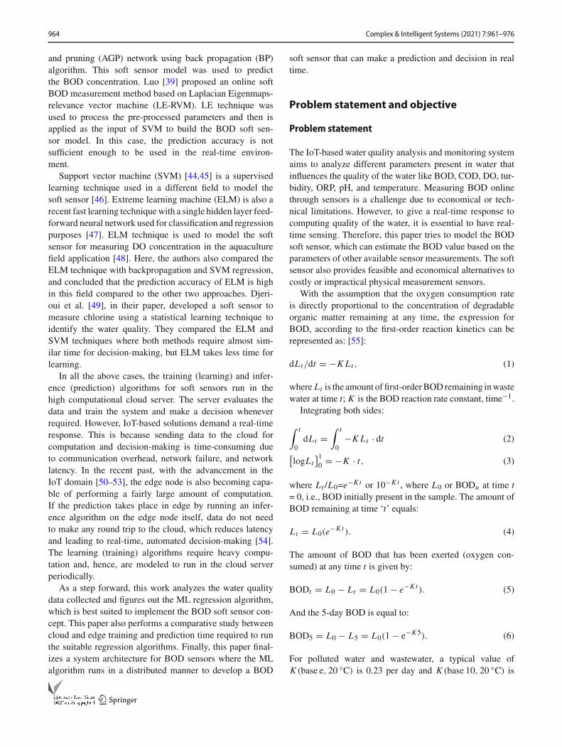
Table 5 Training and prediction time cloud and edge for STP water
ML algorithm Cloud trainingtime (in s)
Edge trainingtime (in s)
Cloud predictiontime (in s)
Edge predictiontime (in s)
Linear regression 0.01 0.05 0.01 0.01
Multi-layer perceptron (1 hidden layer) 0.11 1.74 0.01 0.01
SVM-SMO 0.3 0.52 0.01 0.01
IBK 0.01 0.01 0.01 0.06
KStar 0.01 0.01 0.14 0.6
Random forest 0.05 0.76 0.01 0.03
Random tree 0.01 0.02 0.01 0.01
REPTree 0.01 0.09 0.01 0.01
Table 6 Total prediction time including dual communication time in cloud layer and real-time prediction in edge layer of STP datasets
Training algorithm Prediction fileupload time (ins)
Cloud predictiontime (in s)
Predictionmodel filedownload time(in s)
Total time forcloud end pre-diction (in s)
Edge predictiontime (in s)
Linear regression 0.28 0.01 0.277 0.567 0.01
Multi-layer perceptron (1 hidden layer) 0.28 0.01 0.277 0.567 0.01
SVM-SMO 0.28 0.01 0.277 0.567 0.01
IBK 0.28 0.01 0.277 0.567 0.06
KStar 0.28 0.14 0.277 0.697 0.6
Random forest 0.28 0.01 0.277 0.567 0.03
Random tree 0.28 0.01 0.277 0.567 0.01
REPTree 0.28 0.01 0.277 0.567 0.01
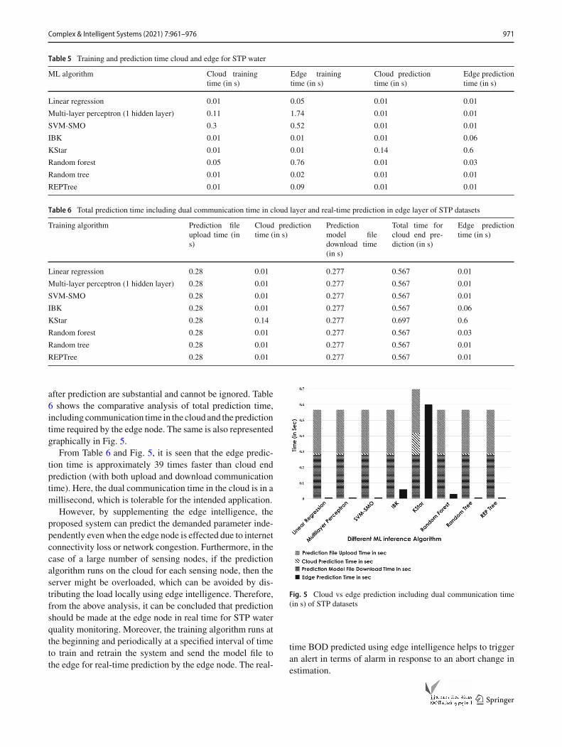
after prediction are substantial and cannot be ignored. Table6 shows the comparative analysis of total prediction time,including communication time in the cloud and the predictiontime required by the edge node. The same is also representedgraphically in Fig. 5.
From Table 6 and Fig. 5, it is seen that the edge predic-tion time is approximately 39 times faster than cloud endprediction (with both upload and download communicationtime). Here, the dual communication time in the cloud is in amillisecond, which is tolerable for the intended application.
However, by supplementing the edge intelligence, theproposed system can predict the demanded parameter inde-pendently evenwhen the edge node is effected due to internetconnectivity loss or network congestion. Furthermore, in thecase of a large number of sensing nodes, if the predictionalgorithm runs on the cloud for each sensing node, then theserver might be overloaded, which can be avoided by dis-tributing the load locally using edge intelligence. Therefore,from the above analysis, it can be concluded that predictionshould be made at the edge node in real time for STP waterquality monitoring. Moreover, the training algorithm runs atthe beginning and periodically at a specified interval of timeto train and retrain the system and send the model file tothe edge for real-time prediction by the edge node. The real-
Fig. 5 Cloud vs edge prediction including dual communication time(in s) of STP datasets
time BOD predicted using edge intelligence helps to triggeran alert in terms of alarm in response to an abort change inestimation.
123

972 Complex & Intelligent Systems (2021) 7:961–976
Table 7 Descriptive statistic ofthe recorded Ganga datasamples
Input (variables) Minimum Maximum Mean Standard deviation
DO (mg/l) 0.14 11.06 6.09 4.13
pH 5.61 8.91 7.519 0.667
Temp (◦C) 9 25.89 18.385 2.666
Turbidity (NTU) 9 136.87 46.821 42.377
BOD (mg/l) 1.26 30.74 12.786 11.345
Table 8 Prediction accuracy inboth cloud and edge for Gangadatasets (by tenfoldcross-validation approach)
Training algorithm Correlation coefficient MAE RMSE RAE (%) RRSE (%)
Linear regression 0.9769 1.3561 2.3962 14.3002 21.3489
Multi-layer perceptron 0.9838 1.0816 2.0174 11.4061 17.974
SVM-SMO 0.9863 0.678 1.8757 7.1499 16.7113
IBK 0.9966 0.143 0.9302 1.497 8.2877
Kstar 0.9929 0.2724 1.3355 2.8728 11.8985
Random forest 0.9905 0.3976 1.5427 4.1932 13.7446
Random tree 0.99 0.3203 1.5845 3.3771 14.1175
REPTree 0.9819 0.6188 2.1273 6.5251 18.9534
Fig. 6 BOD estimation error for experimental setup 2
Table 9 Training and prediction time cloud and edge for Ganga datasets
ML algorithm Cloud trainingtime (in s)
Edge trainingtime (in s)
Cloud predictiontime (in s)
Edge predictiontime (in s)
Linear regression 0.01 0.01 0.01 0.01
Multi-layer perceptron (5 hidden layer) 0.12 1.47 0.01 0.01
SVM-SMO 0.1 1.65 0.01 0.01
IBK 0.01 0.01 0.01 0.04
KStar 0.01 0.01 0.26 0.76
Random forest 0.04 0.55 0.01 0.04
Random tree 0.01 0.01 0.01 0.01
REPTree 0.01 0.09 0.01 0.01
123

Complex & Intelligent Systems (2021) 7:961–976 973
Table 10 Total prediction time including dual communication time in cloud layer and real-time prediction in edge layer for Ganga datasets
Training algorithm Prediction fileupload time (in s)
Cloud predictiontime (in s)
Prediction model filedownload time (in s)
Total time forcloud end pre-diction (in s)
Edge predictiontime (in s)
Linear regression 0.3 0.28 0.01 0.59 0.01
Multi-layer percep-tron (1 hidden layer)
0.3 0.28 0.01 0.59 0.01
SVM-SMO 0.3 0.28 0.01 0.59 0.01
IBK 0.3 0.28 0.01 0.59 0.04
KStar 0.3 0.28 0.26 0.84 0.76
Random forest 0.3 0.28 0.01 0.59 0.04
Random tree 0.3 0.28 0.01 0.59 0.01
REPTree 0.3 0.28 0.01 0.59 0.01
Experimental results and discussion for setup 2
From the experiment setup 1, it is concluded that using fourdifferent physical sensors as input, we can predict the BODin real time. In experiment 2, the same can be tested withreal-time data of the different locations of the Ganga River,hosted by a Government hosted website. Here, we are con-sidering only four sensors data as input data (DO, pH, Temp,and Turbidity) to minimize sensor cost and cross-validate theresult of experiment 1. The collected raw data are stored inthe cloud as well as an edge for further analysis. Here, a totalof 500 samples are taken, and the statistics of the recordedvariables are shown in Table 7.
Soft sensor took four variables datasets as input to predictthe output variable BOD in real time for Ganga River. Thedataset is standardized before it is feed as input for the softsensor model. Here, Table 8 records the performance accu-racy of the ML algorithm to select the appropriate algorithmfor developing soft sensor modeling for Ganga Dataset.
Table 8 depicts the parameters like correlation coeffi-cient, MAE, RMSE, RAE, and RRSE Error after performingtenfold cross-validation with all 500 data points. Here, cross-validation is performed similarly, as done in “ExperimentalResults and Discussions for setup-1”. From the above table,it can observe that for Ganga data points also, IBK (with K= 1) gives better prediction accuracy compared to all otherapproaches. The comparative analysis between actual BODand the predicted BOD in terms of BOD estimation error,MAE, and RMSE using IBK approach are represented inFig. 6. The bar graph of Fig. 6 illustrated the BOD estimationerror of first twofold (i.e., 100 records) and the line graphsrepresent overall MAE and RMSE after performing tenfoldcross-validation approach with the dataset.
To compare the efficiency of different ML algorithms interms of training and prediction time, a total of 500 samplesare taken for training and a single record for prediction. Table
Fig. 7 Cloud vs. edge prediction including dual communication timefor Ganga dataset of experiment 2
9 records the time required to train the dataset and to predictthe result in the cloud and edge layer separately.
From Table 9, it is observed that for all ML algorithms,when the algorithm requires more computation, edge takesmore time for training and prediction compared to the cloud.Table 10 shows the comparative analysis results of total pre-diction time, including communication time in the cloud andthe prediction time at the edge node. The same is also repre-sented graphically in Fig. 7.
From Table 10 and Fig. 7, it is observed that the edge pre-diction time is approximately 31 times faster than the cloudend prediction. From the above analysis, it is verified that theedge can predict the desired parameter independently in realtime. With the consideration of the performance of soft sen-sor modeling for real-time Ganga River data and STP water:the IBK approach is selected tomodel the soft sensor in termsof prediction result accuracy and real-time response. Here,the training algorithm can run offline in the cloud, and theinference algorithm needs to run in edge to achieve a real-time response. As a validation of the complete setup, the
123

974 Complex & Intelligent Systems (2021) 7:961–976
Table 11 Result analysis of real-time deployed system on STP water reservoir
Predictionalgorithm
Correlationcoefficient
MAE RMSE RAE (%) RRSE (%) Cloud prediction Time includ-ing dual communication time(in s)
Edge predictiontime (in s)
IBK 0.9273 0.0812 0.1994 17.20 37.62 0.57 0.15
Fig. 8 BOD estimation error after the system deployment
system is deployed in the STP water outlet of the institute,and real-time BODvalues are predicted and recorded. A totalof 100 real-time values are recorded. The same water sam-ples are collected and tested using the laboratory approachfrom which the actual result are obtained after 5 days, i.e.,BOD5. Figure 8 represents the comparison between 100real-time BOD predicted values by the system with the BODvalue measured through the laboratory approach. The corre-lation coefficient, MAE, RMSE, RAE, and RRSE betweenthe actual and predicted value are calculated and representedin Table 11.
From Table 11, it is observed that the calculated correla-tion coefficient between actual and predicted data using IBKwith K = 1 is high, i.e., 0.9273. MAE and RMSE are lowas per the requirement. The BOD estimation error is alsorepresented through the bar graph, as shown in Fig. 8. Thecalculated MAE and RMSE are also shown in Fig. 8 throughline graph. The average prediction time in the cloud, includ-ing uploading and downloading time, is quite higher than theaverage prediction time at the edge.
Conclusions and future scope
Soft sensors have a practical impact on the design and devel-opment of IoT-based water quality monitoring system. Thispaper presents a BOD soft sensormodel that uses data-drivenML techniques to estimate the value of BOD in real time.A comparative study between different ML algorithms wascarried out to select a suitable regression technique for the
proposed system and it was found that the IBK algorithm isa good fit. A comparison between cloud level and edge leveltraining and required prediction time is made to estimatethe values in real time. It is found that estimation time foredge-based algorithms, which uses intelligence at the edge topredict the BOD values, is within a tolerable limit to make adecisions in comparison to the cloud based models. Finally,the real-time water quality monitoring system is designedusing different physical hardware sensors and BOD soft sen-sor. The BOD soft sensor is modeled using the IBK approachwith edge intelligence, which impacts directly on the cost ofthe system, and real-time response time. Based on this study,we can make decisions and take necessary actions as well ascontrol the water quality monitoring system in real time. Wealso propose to develop soft sensor models for other waterand air quality parameters in the future.
Acknowledgements This research is partially supported by WOS-A,ITRA, MEITY, Govt. of India and IUSSTF of Department of Scienceand Technology, Govt. of India
Open Access This article is licensed under a Creative CommonsAttribution 4.0 International License, which permits use, sharing, adap-tation, distribution and reproduction in any medium or format, aslong as you give appropriate credit to the original author(s) and thesource, provide a link to the Creative Commons licence, and indi-cate if changes were made. The images or other third party materialin this article are included in the article’s Creative Commons licence,unless indicated otherwise in a credit line to the material. If materialis not included in the article’s Creative Commons licence and yourintended use is not permitted by statutory regulation or exceeds thepermitted use, youwill need to obtain permission directly from the copy-
123

Complex & Intelligent Systems (2021) 7:961–976 975
right holder. To view a copy of this licence, visit http://creativecommons.org/licenses/by/4.0/.
References
1. Li C, Zhang B, Luo P, Shi H, Li L, Gao Y, Lee CT, Zhang Z, WuW-M (2019) Performance of a pilot-scale aquaponics system usinghydroponics and immobilized biofilm treatment for water qualitycontrol. J Clean Prod 208:274–284
2. W H Organization (2017) Guidelines for drinking-water quality,4th edition, incorporating the 1st addendum. [Online]. https://apps.who.int/iris/bitstream/handle/10665/254637/9789241549950-eng.pdf
3. Qiao J, Hu Z, Li W (2016) Soft measurement modelling basedon chaos theory for biochemical oxygen demand (BOD). Water8(12):581
4. Saberi-Movahed F, NajafzadehM,Mehrpooya A (2020) Receivingmore accurate predictions for longitudinal dispersion coefficientsin water pipelines: training group method of data handling usingextreme learning machine conceptions. Water Resour Manag34(2):529–561
5. Najafzadeh M, Ghaemi A, Emamgholizadeh S (2019) Predictionof water quality parameters using evolutionary computing-basedformulations. Int J Environ Sci Technol 16(10):6377–6396
6. Najafzadeh M, Ghaemi A (2019) Prediction of the five-day bio-chemical oxygen demand and chemical oxygen demand in naturalstreams using machine learning methods. Environ Monit Assess191(6):380
7. Najafzadeh M, Tafarojnoruz A (2016) Evaluation of neuro-fuzzyGMDH-based particle swarm optimization to predict longitudinaldispersion coefficient in rivers. Environ Earth Sci 75(2):157
8. ChowduryMSU, Emran TB, Ghosh S, PathakA, AlamMM,AbsarN,AnderssonK,HossainMS (2019) Iot based real-time river waterquality monitoring system. Procedia Comput Sci 155:161–168
9. Tripathy AK, Das TK, Chowdhary CL (2019) Monitoring qual-ity of tap water in cities using IoT. In: Subramanian B, ChenSS, Reddy K (eds) Emerging technologies for agriculture andenvironment. Lecture notes on multidisciplinary industrial engi-neering. Springer, Singapore, pp 107–113. https://doi.org/10.1007/978-981-13-7968-0_8
10. Encinas C, Ruiz E, Cortez J, Espinoza A (2017) Design and imple-mentation of a distributed IOT system for the monitoring of waterquality in aquaculture. In: 2017 wireless telecommunications sym-posium (WTS). IEEE, Chicago, IL, 26–28 April 2017, pp 1–7
11. BannaMH,NajjaranH, SadiqR, ImranSA,RodriguezMJ,HoorfarM (2014) Miniaturized water quality monitoring pH and conduc-tivity sensors. Sens Actuators B Chem 193:434–441
12. Zhuiykov S (2012) Solid-state sensors monitoring parameters ofwater quality for the next generation of wireless sensor networks.Sens Actuators B Chem 161(1):1–20
13. Sagar S, Chavan R, Patil C, Shinde D, Kekane S (2015) Physico-chemical parameters for testing of water: a review. Int J Chem Stud3(4):24–28
14. Murphy K, Heery B, Sullivan T, Zhang D, Paludetti L, Lau KT,Diamond D, Costa E, Regan F et al (2015) A low-cost autonomousoptical sensor for water quality monitoring. Talanta 132:520–27
15. Curreri F, Fiumara G, Xibilia MG (2020) Input selection methodsfor soft sensor design: a survey. Future Internet 12(6):97
16. Fortuna L, Graziani S, RizzoA, XibiliaMG (2007) Soft sensors formonitoring and control of industrial processes. Springer, London
17. Kadlec P, Gabrys B, Strandt S (2009) Data-driven soft sensors inthe process industry. Comput Chem Eng 33(4):795–814
18. Pani AK, Vadlamudi VK, Mohanta HK (2013) Development andcomparison of neural network based soft sensors for online esti-mation of cement clinker quality. ISA Trans 52(1):19–29
19. HaimiH,MulasM, Corona F, Vahala R (2013) derived soft-sensorsfor biological wastewater treatment plants: an overview. EnvironModel Softw 47:88–107
20. Huang M, Ma Y, Wan J, Chen X (2015) A sensor-software basedon a genetic algorithm-based neural fuzzy system for modellingand simulating a waste water treatment process. Appl Soft Comput27:1–10
21. Wei W, Changhui D, Xiangjun L, Jun G (2017) Soft-sensor soft-ware designof dissolvedoxygen in aquaculture.ChinAutomCongr2017:5413–17
22. Tang J, Quek TQ (2016) The role of cloud computing in content-centric mobile networking. IEEE Commun Mag 54(8):52–59
23. Corcoran P, Datta SK (2016) Mobile-edge computing and theinternet of things for consumers: extending cloud computing andservices to the edge of the network. IEEE Consum Electron Mag5(4):73–74
24. Vallati C, Virdis A, Mingozzi E, Stea G (2016) Mobile-edge com-puting come home connecting things in future smart homes usinglte device-to-device communications. IEEEConsumElectronMag5(4):77–83
25. Shi W, Cao J, Zhang Q, Li Y, Xu L (2016) Edge computing: visionand challenges. IEEE Internet Things J 3(5):637–646
26. Sharma SK, Wang X (2017) Live data analytics with collaborativeedge and cloud processing in wireless iot networks. IEEE Access5:4621–4635
27. Kadlec P, Gabrys B, Strandt S, Data-Kadlec P (2009) Data-drivensoft sensors in the process industry. Comput Chem Eng 33(4):795–814
28. Sharma S, Tambe SS (2014) Soft-sensor development for bio-chemical systems using genetic programming. Biochem Eng J85:89–100
29. Sagmeister P, Wechselberger P, Jazini M, Meitz A, Langemann T,Herwig C (2013) Soft sensor assisted dynamic bioprocess control:efficient tools for bioprocess development. Chem Eng Sci 96:190–98
30. Rato TJ, Reis MS (2018) Building optimal multiresolution softsensors for continuous processes. Ind Eng ChemRes 57(30):9750–9765
31. Lu J, Liu A, Song Y, Zhang G (2020) Data-driven decision sup-port under concept drift in streamed big data. Complex Intell Syst6(1):157–163
32. Jolliffe IT, Cadima J (2016) Principal component analysis: a reviewand recent developments. Philos Trans R Soc AMath Phys Eng Sci374(2065):20150202
33. Shang C, Yang F, Huang D, Lyu W (2014) Data-driven soft sensordevelopment based on deep learning technique. J Process Control24(3):223–233
34. Jang J-SR, Sun C-T, Mizutani E (1997) Neuro-fuzzy and soft com-puting: a computational approach to learning and machine intel-ligence [book review]. IEEE Trans Autom Control 42(10):1482–1484
35. Smusz S, Kurczab R, Bojarski AJ (2013) Amultidimensional anal-ysis of machine learning methods performance in the classificationof bioactive compounds. Chemom Intell Lab Syst 128:89–100
36. Yan W, Shao H, Wang X (2004) Soft sensing modeling based onsupport vector machine and Bayesian model selection. ComputChem Eng 28(8):1489–1498
37. Liu Y, Chen T, Chen J (2015) Auto-switch gaussian processregression-basedprobabilistic soft sensors for industrialmultigradeprocesses with transitions. Ind Eng Chem Res 54(18):5037–5047
38. Chen J, Yu J, Zhang Y (2014) Multivariate video analysis andgaussian process regression model based soft sensor for online
123

976 Complex & Intelligent Systems (2021) 7:961–976
estimation andpredictionof nickel pellet size distributions.ComputChem Eng 64:13–23
39. Luo L (2016) Biochemical oxygen demand soft measurementbased on le-rvm. In: 2nd 2016 international conference on sus-tainable development (ICSD 2016). Atlantis Press, Xi’an, China,2–4December 2016, pp 164–167. https://doi.org/10.2991/icsd-16.2017.35
40. Lamrini B, BenhammouA, Le LannM-V,KaramaA (2005) A neu-ral software sensor for online prediction of coagulant dosage in adrinkingwater treatment plant. Trans InstMeasControl 27(3):195–213
41. Wang L, Shao C,Wang H,Wu H (2006) Radial basis function neu-ral networks-based modeling of the membrane separation process:hydrogen recovery from refinery gases. JNatGasChem15(3):230–234
42. JuntunenP, LiukkonenM,LehtolaMJ,HiltunenY (2013)Dynamicsoft sensors for detecting factors affecting turbidity in drinkingwater. J Hydroinform 15(2):416–426
43. Zhang M et al (2011) Research on dynamic feed-forward neuralnetwork structure based on growing and pruningmethods. ZhinengXitong Xuebao 6:101–06
44. Cristianini N, Shawe-Taylor J et al (2000) An introduction to sup-port vector machines and other kernel-based learning methods.Cambridge University Press, Cambridge
45. Cortes C, Vapnik V (1995) Support vector networks. Mach Learn20(3):273–97
46. Yan W, Shao H, Wang X (2004) Soft sensing modeling based onsupport vector machine and Bayesian model selection. ComputChem Eng 28(8):1489–98
47. HuangG-B, ZhuQ-Y, SiewC-K (2006) Extreme learningmachine:theory and applications. Neurocomputing 70(1–3):489–501
48. WangW, Deng C, Li X (2014) Soft sensing of dissolved oxygen infishpond via extreme learning machine. In: Proceeding of the 11thworld congress on intelligent control and automation, Shenyang.pp 3393–3395. https://doi.org/10.1109/WCICA.2014.7053278
49. Djerioui M, Bouamar M, Ladjal M, Zerguine A (2019) Chlorinesoft sensor based on extreme learning machine for water qualitymonitoring. Arab J Sci Eng 44(3):2033–2044
50. Xia F, Yang LT, Wang L, Vinel A (2012) Internet of things. Int JCommun Syst 25(9):1101–02
51. KopetzH (2011) Internet of things. In:Real-time systems. Springer,Boston, MA, pp 307–323
52. Atzori L, IeraA,MorabitoG (2010)The internet of things: a survey.Comput Netw 54(15):2787–805
53. Gomathi P,Baskar S, Shakeel PM (2020)Concurrent service accessand management framework for user-centric future internet ofthings in smart cities. Complex Intell Syst. https://doi.org/10.1007/s40747-020-00160-5
54. Ovenden J (2018) Edge computing and the future of machinelearning | articles | big data. Innovation enterprise. DIA-LOG. https://channels.theinnovationenterprise.com/articles/why-machine-learning-needs-edge-computing. Accessed 23 Jan 2019
55. Ghangrekar M (2019) Bod model. IIT Kharagpur. DIALOG.https://scetcivil.weebly.com/uploads/5/3/9/5/5395830/m9_l12-water_quality_and_estimation_of_organic_content-contd.pdf.Accessed 24 Jan 2019
56. Draper NR, Smith H (1998) Applied regression analysis, vol 326.Wiley, New York
57. Najafzadeh M, Oliveto G (2020) Riprap incipient motion forover-topping flows with machine learning models. J Hydroinform22(4):749–767
58. SadeghiG,NajafzadehM,AmeriM (2020)Thermal characteristicsof evacuated tube solar collectors with coil inside: an experimentalstudy and evolutionary algorithms. Renew Energy 151:575–588
59. Souza FA, Araújo R, Mendes J (2016) Review of soft sensor meth-ods for regression applications. Chemom Intell LabSyst 152:69–79
60. Vapnik V (2013) The nature of statistical learning theory. Springerscience & business media, Berlin
Publisher’s Note Springer Nature remains neutral with regard to juris-dictional claims in published maps and institutional affiliations.
123