machine learning for automated reasoningkuehlwein/preprints/phdthesisdanielkuehlwein.pdf · machine...
TRANSCRIPT
Machine Learning for Automated Reasoning
Proefschrift
ter verkrijging van de graad van doctoraan de Radboud Universiteit Nijmegen,
op gezag van de rector magnificus prof. mr. S.C.J.J. Kortmann,volgens besluit van het college van decanen
in het openbaar te verdedigen op maandag 14 april 2014om 10:30 uur precies
door
Daniel A. Kühlwein
geboren op 7 november 1982te Balingen, Duitsland
Promotoren:
Prof. dr. Tom Heskes
Prof. dr. Herman Geuvers
Copromotor:
Dr. Josef Urban
Manuscriptcommissie:
Prof. dr. M.C.J.D. van Eekelen (Open University, the Netherlands)Prof. dr. L.C. Paulson (University of Cambridge, UK)Dr. S. Schulz (TU Munich, Germany)
This research was supported by the NWO project Learning2Reason (612.001.010).
Copyright© 2013 Daniel Kühlwein
ISBN 978-94-6259-132-5Gedrukt door Ipskamp Drukkers, Nijmegen

Contents
Contents i
1 Introduction 11.1 Formal Mathematics . . . . . . . . . . . . . . . . . . . . . . . . . . . . 1
1.1.1 Interactive Theorem Proving . . . . . . . . . . . . . . . . . . . . 11.1.2 Automated Theorem Proving . . . . . . . . . . . . . . . . . . . . 21.1.3 Industrial Applications . . . . . . . . . . . . . . . . . . . . . . . 31.1.4 Learning to Reason . . . . . . . . . . . . . . . . . . . . . . . . . 4
1.2 Machine Learning in a Nutshell . . . . . . . . . . . . . . . . . . . . . . 51.3 Outline of this Thesis . . . . . . . . . . . . . . . . . . . . . . . . . . . . 6
2 Premise Selection in ITPs as a Machine Learning Problem 92.1 Premise Selection as a Machine-Learning Problem . . . . . . . . . . . . 9
2.1.1 The Training Data . . . . . . . . . . . . . . . . . . . . . . . . . 102.1.2 What to Learn . . . . . . . . . . . . . . . . . . . . . . . . . . . 102.1.3 Features . . . . . . . . . . . . . . . . . . . . . . . . . . . . . . . 12
2.2 Naive Bayes and Kernel-Based Learning . . . . . . . . . . . . . . . . . . 142.2.1 Formal Setting . . . . . . . . . . . . . . . . . . . . . . . . . . . 142.2.2 A Naive Bayes Classifier . . . . . . . . . . . . . . . . . . . . . . 152.2.3 Kernel-based Learning . . . . . . . . . . . . . . . . . . . . . . . 152.2.4 Multi-Output Ranking . . . . . . . . . . . . . . . . . . . . . . . 18
2.3 Challenges . . . . . . . . . . . . . . . . . . . . . . . . . . . . . . . . . . 192.3.1 Features . . . . . . . . . . . . . . . . . . . . . . . . . . . . . . . 202.3.2 Dependencies . . . . . . . . . . . . . . . . . . . . . . . . . . . . 202.3.3 Online Learning and Speed . . . . . . . . . . . . . . . . . . . . . 21
3 Overview of Premise Selection Techniques 233.1 Premise Selection Algorithms . . . . . . . . . . . . . . . . . . . . . . . 23
3.1.1 Premise Selection Setting . . . . . . . . . . . . . . . . . . . . . 233.1.2 Learning-based Ranking Algorithms . . . . . . . . . . . . . . . . 243.1.3 Other Algorithms Used in the Evaluation . . . . . . . . . . . . . 25
i
CONTENTS
3.1.4 Techniques Not Included in the Evaluation . . . . . . . . . . . . 253.2 Machine Learning Evaluation Metrics . . . . . . . . . . . . . . . . . . . 263.3 Evaluation . . . . . . . . . . . . . . . . . . . . . . . . . . . . . . . . . . 27
3.3.1 Evaluation Data . . . . . . . . . . . . . . . . . . . . . . . . . . . 273.3.2 Machine Learning Evaluation . . . . . . . . . . . . . . . . . . . 283.3.3 ATP Evaluation . . . . . . . . . . . . . . . . . . . . . . . . . . . 30
3.4 Combining Premise Rankers . . . . . . . . . . . . . . . . . . . . . . . . 333.5 Conclusion . . . . . . . . . . . . . . . . . . . . . . . . . . . . . . . . . 34
4 Learning from Multiple Proofs 374.1 Learning from Different Proofs . . . . . . . . . . . . . . . . . . . . . . . 374.2 The Machine Learning Framework and the Data . . . . . . . . . . . . . . 384.3 Using Multiple Proofs . . . . . . . . . . . . . . . . . . . . . . . . . . . . 39
4.3.1 Substitutions and Unions . . . . . . . . . . . . . . . . . . . . . . 404.3.2 Premise Averaging . . . . . . . . . . . . . . . . . . . . . . . . . 404.3.3 Premise Expansion . . . . . . . . . . . . . . . . . . . . . . . . . 41
4.4 Results . . . . . . . . . . . . . . . . . . . . . . . . . . . . . . . . . . . . 424.4.1 Experimental Setup . . . . . . . . . . . . . . . . . . . . . . . . . 424.4.2 Substitutions and Unions . . . . . . . . . . . . . . . . . . . . . . 424.4.3 Premise Averaging . . . . . . . . . . . . . . . . . . . . . . . . . 424.4.4 Premise Expansions . . . . . . . . . . . . . . . . . . . . . . . . 444.4.5 Other ATPs . . . . . . . . . . . . . . . . . . . . . . . . . . . . . 444.4.6 Comparison With the Best Results Obtained so far . . . . . . . . 464.4.7 Machine Learning Evaluation . . . . . . . . . . . . . . . . . . . 46
4.5 Conclusion . . . . . . . . . . . . . . . . . . . . . . . . . . . . . . . . . 48
5 Automated and Human Proofs in General Mathematics 495.1 Introduction: Automated Theorem Proving in Mathematics . . . . . . . . 495.2 Finding proofs in the MML with AI/ATP support . . . . . . . . . . . . . 50
5.2.1 Mining the dependencies from all MML proofs . . . . . . . . . . 505.2.2 Learning Premise Selection from Proof Dependencies . . . . . . 515.2.3 Using ATPs to Prove the Conjectures from the Selected Premises 52
5.3 Proof Metrics . . . . . . . . . . . . . . . . . . . . . . . . . . . . . . . . 535.4 Evaluation . . . . . . . . . . . . . . . . . . . . . . . . . . . . . . . . . . 54
5.4.1 Comparing weights . . . . . . . . . . . . . . . . . . . . . . . . . 565.5 Conclusion . . . . . . . . . . . . . . . . . . . . . . . . . . . . . . . . . 56
6 MaSh - Machine Learning for Sledgehammer 596.1 Introduction . . . . . . . . . . . . . . . . . . . . . . . . . . . . . . . . . 596.2 Sledgehammer and MePo . . . . . . . . . . . . . . . . . . . . . . . . . . 616.3 The Machine Learning Engine . . . . . . . . . . . . . . . . . . . . . . . 62
6.3.1 Basic Concepts . . . . . . . . . . . . . . . . . . . . . . . . . . . 636.3.2 Input and Output . . . . . . . . . . . . . . . . . . . . . . . . . . 636.3.3 The Learning Algorithm . . . . . . . . . . . . . . . . . . . . . . 63
ii
CONTENTS
6.4 Integration in Sledgehammer . . . . . . . . . . . . . . . . . . . . . . . . 646.4.1 The Low-Level Learner Interface . . . . . . . . . . . . . . . . . 646.4.2 Learning from and for Isabelle . . . . . . . . . . . . . . . . . . . 656.4.3 Relevance Filters: MaSh and MeSh . . . . . . . . . . . . . . . . 676.4.4 Automatic and Manual Control . . . . . . . . . . . . . . . . . . 686.4.5 Nonmonotonic Theory Changes . . . . . . . . . . . . . . . . . . 68
6.5 Evaluations . . . . . . . . . . . . . . . . . . . . . . . . . . . . . . . . . 696.5.1 Evaluation on Large Formalizations . . . . . . . . . . . . . . . . 696.5.2 Judgment Day . . . . . . . . . . . . . . . . . . . . . . . . . . . 72
6.6 Related Work and Contributions . . . . . . . . . . . . . . . . . . . . . . 736.7 Conclusion . . . . . . . . . . . . . . . . . . . . . . . . . . . . . . . . . 73
7 MaLeS - Machine Learning of Strategies 757.1 Introduction: ATP Strategies . . . . . . . . . . . . . . . . . . . . . . . . 75
7.1.1 The Strategy Selection Problem . . . . . . . . . . . . . . . . . . 767.1.2 Overview . . . . . . . . . . . . . . . . . . . . . . . . . . . . . . 77
7.2 Finding Good Search Strategies with MaLeS . . . . . . . . . . . . . . . 777.3 Strategy Scheduling with MaLeS . . . . . . . . . . . . . . . . . . . . . . 79
7.3.1 Notation . . . . . . . . . . . . . . . . . . . . . . . . . . . . . . 807.3.2 Features . . . . . . . . . . . . . . . . . . . . . . . . . . . . . . . 807.3.3 Runtime Prediction Functions . . . . . . . . . . . . . . . . . . . 827.3.4 Crossvalidation . . . . . . . . . . . . . . . . . . . . . . . . . . . 857.3.5 Creating Schedules from Prediction Functions . . . . . . . . . . . 85
7.4 Evaluation . . . . . . . . . . . . . . . . . . . . . . . . . . . . . . . . . . 867.4.1 E-MaLeS . . . . . . . . . . . . . . . . . . . . . . . . . . . . . . 877.4.2 Satallax-MaLeS . . . . . . . . . . . . . . . . . . . . . . . . . . . 887.4.3 LEO-MaLeS . . . . . . . . . . . . . . . . . . . . . . . . . . . . 917.4.4 Further Remarks . . . . . . . . . . . . . . . . . . . . . . . . . . 947.4.5 CASC . . . . . . . . . . . . . . . . . . . . . . . . . . . . . . . . 95
7.5 Using MaLeS . . . . . . . . . . . . . . . . . . . . . . . . . . . . . . . . 977.5.1 E-MaLeS, LEO-MaLeS and Satallax-MaLeS . . . . . . . . . . . 977.5.2 Tuning E, LEO-II or Satallax for a New Set of Problems . . . . . 987.5.3 Using a New Prover . . . . . . . . . . . . . . . . . . . . . . . . 101
7.6 Future Work . . . . . . . . . . . . . . . . . . . . . . . . . . . . . . . . . 1027.7 Conclusion . . . . . . . . . . . . . . . . . . . . . . . . . . . . . . . . . 102
Contributions 105
Bibliography 107
Scientific Curriculum Vitae 121
Summary 125
iii

CONTENTS
Samenvatting 127
Acknowledgments 129
iv
Chapter 1
Introduction
Heuristically, a proof is a rhetorical device for convincing someone else thata mathematical statement is true or valid.
— Steven G. Krantz, [52]I am entirely convinced that formal verification of mathematics will eventu-ally become commonplace.
— Jeremy Avigad, [6]
1.1 Formal Mathematics
The foundations of modern mathematics were laid at the end of the 19th century and thebeginning of the 20th century. Seminal works such as Frege’s Begriffsschrift [30] estab-lished the notion of mathematical proofs as formal derivations in a logical calculus. InPrincipia Mathematica [118], Whitehead and Russell set out to show by example thatall of mathematics can be derived from a small set of axioms using an appropriate log-ical calculus. Even though Gödel later showed that no effectively generated consistentaxiom system can capture all mathematical truth [32], Principia Mathematica showedthat most of normal mathematics can indeed be catered for by a formal system. Proofscould now be rigidly defined, and verifying the validity of a proof was a simple matter ofchecking whether the rules of the calculus were correctly applied. But formal proofs wereextremely tedious to write (and read), and so they found no audience among practicingmathematicians.
1.1.1 Interactive Theorem Proving
With the advent of computers, formal mathematics became a more realistic proposal.Interactive theorem provers (ITP), or proof assistants, are computer programs that support
This chapter is based on: “A Survey of Axiom Selection as a Machine Learning Problem”, submitted to“Infinity, computability, and metamathematics. Festschrift celebrating the 60th birthdays of Peter Koepke andPhilip Welch”.
1
CHAPTER 1. INTRODUCTION
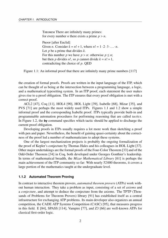
Theorem There are infinitely many primes:for every number n there exists a prime p > n.
Proof [after Euclid]Given n. Consider k = n! + 1, where n! = 1 ·2 ·3 · . . . ·n.Let p be a prime that divides k.For this number p we have p > n: otherwise p ≤ n;but then p divides n!, so p cannot divide k = n! + 1,contradicting the choice of p. QED
Figure 1.1: An informal proof that there are infinitely many prime numbers [117]
the creation of formal proofs. Proofs are written in the input language of the ITP, whichcan be thought of as being at the intersection between a programming language, a logic,and a mathematical typesetting system. In an ITP proof, each statement the user makesgives rise to a proof obligation. The ITP ensures that every proof obligation is met with acorrect proof.
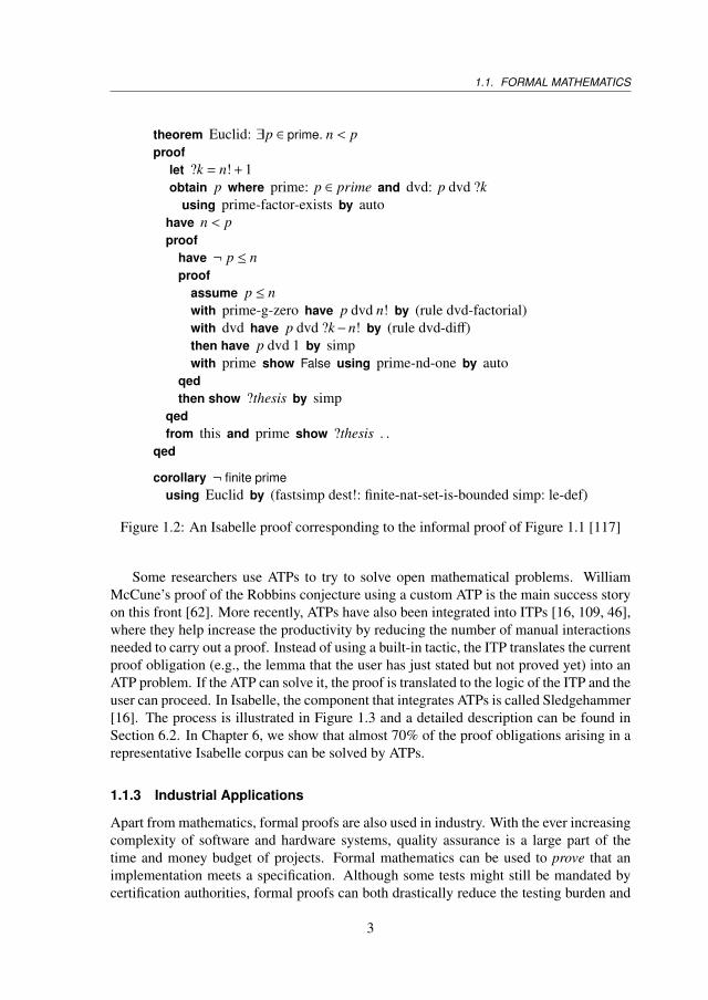
ACL2 [47], Coq [11], HOL4 [90], HOL Light [39], Isabelle [68], Mizar [35], andPVS [71] are perhaps the most widely used ITPs. Figures 1.1 and 1.2 show a simpleinformal proof and the corresponding Isabelle proof. ITPs typically provide built-in andprogrammable automation procedures for performing reasoning that are called tactics.In Figure 1.2, the by command specifies which tactic should be applied to discharge thecurrent proof obligation.
Developing proofs in ITPs usually requires a lot more work than sketching a proofwith pen and paper. Nevertheless, the benefit of gaining quasi-certainty about the correct-ness of the proof led a number of mathematicians to adopt these systems.
One of the largest mechanization projects is probably the ongoing formalization ofthe proof of Kepler’s conjecture by Thomas Hales and his colleagues in HOL Light [37].Other major undertakings are the formal proofs of the Four-Color Theorem [33] and of theOdd-Order Theorem [34] in Coq, both developed under Georges Gonthier’s leadership.In terms of mathematical breadth, the Mizar Mathematical Library [61] is perhaps themain achievement of the ITP community so far: With nearly 52000 theorems, it covers alarge portion of the mathematics taught at the undergraduate level.
1.1.2 Automated Theorem Proving
In contrast to interactive theorem provers, automated theorem provers (ATPs) work with-out human interaction. They take a problem as input, consisting of a set of axioms anda conjecture, and attempt to deduce the conjecture from the axioms. The TPTP (Thou-sands of Problems for Theorem Provers) library [91] has established itself as a centralinfrastructure for exchanging ATP problems. Its main developer also organizes an annualcompetition, the CADE ATP Systems Competition (CASC) [95], that measures progressin this field. E [84], SPASS [114], Vampire [77], and Z3 [66] are well-known ATPs forclassical first-order logic.
2
1.1. FORMAL MATHEMATICS
theorem Euclid: ∃p ∈ prime. n < pproof
let ?k = n! + 1obtain p where prime: p ∈ prime and dvd: p dvd ?k
using prime-factor-exists by autohave n < pproof
have ¬ p ≤ nproof
assume p ≤ nwith prime-g-zero have p dvd n! by (rule dvd-factorial)with dvd have p dvd ?k−n! by (rule dvd-diff)then have p dvd 1 by simpwith prime show False using prime-nd-one by auto
qedthen show ?thesis by simp
qedfrom this and prime show ?thesis . .
qed
corollary ¬ finite primeusing Euclid by (fastsimp dest!: finite-nat-set-is-bounded simp: le-def)
Figure 1.2: An Isabelle proof corresponding to the informal proof of Figure 1.1 [117]
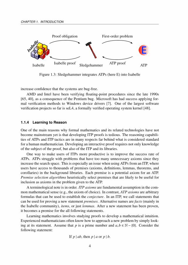
Some researchers use ATPs to try to solve open mathematical problems. WilliamMcCune’s proof of the Robbins conjecture using a custom ATP is the main success storyon this front [62]. More recently, ATPs have also been integrated into ITPs [16, 109, 46],where they help increase the productivity by reducing the number of manual interactionsneeded to carry out a proof. Instead of using a built-in tactic, the ITP translates the currentproof obligation (e.g., the lemma that the user has just stated but not proved yet) into anATP problem. If the ATP can solve it, the proof is translated to the logic of the ITP and theuser can proceed. In Isabelle, the component that integrates ATPs is called Sledgehammer[16]. The process is illustrated in Figure 1.3 and a detailed description can be found inSection 6.2. In Chapter 6, we show that almost 70% of the proof obligations arising in arepresentative Isabelle corpus can be solved by ATPs.
1.1.3 Industrial Applications
Apart from mathematics, formal proofs are also used in industry. With the ever increasingcomplexity of software and hardware systems, quality assurance is a large part of thetime and money budget of projects. Formal mathematics can be used to prove that animplementation meets a specification. Although some tests might still be mandated bycertification authorities, formal proofs can both drastically reduce the testing burden and
3
CHAPTER 1. INTRODUCTION
Isabelle Sledgehammer ATP
Proof obligation First-order problem
Isabelle proof ATP proof
Figure 1.3: Sledgehammer integrates ATPs (here E) into Isabelle
increase confidence that the systems are bug-free.AMD and Intel have been verifying floating-point procedures since the late 1990s
[65, 40], as a consequence of the Pentium bug. Microsoft has had success applying for-mal verification methods to Windows device drivers [7]. One of the largest softwareverification projects so far is seL4, a formally verified operating system kernel [48].
1.1.4 Learning to Reason
One of the main reasons why formal mathematics and its related technologies have notbecome mainstream yet is that developing ITP proofs is tedious. The reasoning capabili-ties of ATPs and ITP tactics are in many respects far behind what is considered standardfor a human mathematician. Developing an interactive proof requires not only knowledgeof the subject of the proof, but also of the ITP and its libraries.
One way to make users of ITPs more productive is to improve the success rate ofATPs. ATPs struggle with problems that have too many unnecessary axioms since theyincrease the search space. This is especially an issue when using ATPs from an ITP, whereusers have access to thousands of premises (axioms, definitions, lemmas, theorems, andcorollaries) in the background libraries. Each premise is a potential axiom for an ATP.Premise selection algorithms heuristically select premises that are likely to be useful forinclusion as axioms in the problem given to the ATP.
A terminological note is in order. ITP axioms are fundamental assumption in the com-mon mathematical sense (e.g., the axiom of choice). In contrast, ATP axioms are arbitraryformulas that can be used to establish the conjecture. In an ITP, we call statements thatcan be used for proving a new statement premises. Alternative names are facts (mainly inthe Isabelle community), items, or just lemmas. After a new statement has been proven,it becomes a premise for the all following statements.
Learning mathematics involves studying proofs to develop a mathematical intuition.Experienced mathematicians often know how to approach a new problem by simply look-ing at its statement. Assume that p is a prime number and a,b ∈ N− {0}. Consider thefollowing statement:
If p | ab, then p | a or p | b.
4
1.2. MACHINE LEARNING IN A NUTSHELL
Even though mathematicians usually know about many different areas (e.g., linear alge-bra, probability theory, numerics, analysis), when trying to prove the above statementthey would ignore those areas and rely on their knowledge about number theory. At anabstract level, they perform premise selection to reduce their search space.
Most common premise selection algorithms rely on (recursively) comparing the sym-bols and terms of the conjecture and axioms [41, 64]. For example, if the conjectureinvolves π and sin, they will prefer axioms that also talk about either of these two sym-bols, ideally both. The main drawback of such approaches is that they focus exclusivelyon formulas, ignoring the rich information contained in proofs. In particular, they do notlearn from previous proofs.
1.2 Machine Learning in a Nutshell
This section aims to provide a high-level introduction to machine learning; for a morethorough discussion, we refer to standard textbooks [13, 60, 67]. Machine learning con-cerns itself with extracting information from data. Some typical examples of machinelearning problems are listed below.
Spam classification: Predict if a new email is spam.
Face detection: Find human faces in a picture.
Web search: Predict the websites that contain the information the user is looking for.
The results of a learning algorithm is a prediction function that takes a new datapoint(email, picture, search query) and returns a target value (spam / not spam, location offaces, relevant websites). The learning is done by optimizing a score function over atraining dataset. Typical score functions are accuracy (how many emails were correctlylabeled?) and the root mean square error (the Euclidean distance between the predictedvalues and the real values). Elements of the training datasets are datapoints together withtheir intended value. For example:
Spam classification: A set of emails together with their classification.
Face detection: A set of pictures where all faces are marked.
Web search: A set of query-relevant websites tuples.
The performance of the learned function heavily depends on the quality of the trainingdata, as expressed by the aphorism “Garbage in, garbage out.” If the training data is notrepresentative for the problem, the prediction function will likely not generalize to newdata.
In addition to the training data, problem features are also essential. Features are theinput of the prediction function and should describe the relevant attributes of the data-point. A datapoint can have several possible feature representations. Feature engineeringconcerns itself with identifying relevant features [59]. To simplify computations, most
5
CHAPTER 1. INTRODUCTION
machine learning algorithms require that the features are a (sparse) real-valued vector.Potential features are listed below.
Spam classification: A list of all the words occurring in the email.
Face detection: The matrix containing the color values of the pixels.
Web search: The n-grams of the query.
From a mathematical point of view, most machine learning problems can be reducedto an optimization problem. Let D ⊆ X ×T be a training dataset consisting of datapointsand their corresponding target value. Let ϕ : X → F be a feature function that maps adatapoint to its feature representation in the feature space F (usually a subset of Rn forsome n ∈ N). Furthermore, let F ⊆ (F→ T ) be a set of functions that map features to thetarget space and s a (convex) score function s : D×F → R. One possible goal is to findthe function f ∈ F that maximizes the average score over the training set D. The maindifferences between various learning algorithms are the function space F and the scorefunction s they use.
If the function space is too expressive, overfitting may occur: The learned functionf ∈ F might perform well on the training data D, but poorly on unseen data. A simpleexample is trying to fit a polynomial of degree n− 1 through n training datapoints; thiswill give perfect scores on the training data but is likely to yield a curve that behaves sowildly as to be useless to make predictions.
Regularization is used to balance function complexity with the result of the scorefunction. To estimate how well a learning algorithm generalizes or to tune metaparame-ters (e.g., which prior to use in a Bayesian model ), cross-validation partitions the trainingdata in two sets: one set used for training, the other for the evaluation. Section 2.2.4 givesan example of metaparameter tuning with cross-validation.
1.3 Outline of this Thesis
This work develops machine learning methods that can be used to improve both interac-tive and automated theorem proving. The first part of the thesis focuses on how learningfrom previous proofs can help to improve premise selection algorithms. In a way, we aretrying to teach the computer mathematical intuition. The second part concerns itself withthe orthogonal problem of strategy selection for ATPs. My detailed contributions to thethesis chapters are listed in the Contributions section 7.7.
Chapter 2 presents premise selection as a machine learning problem, an idea originallyintroduced in [101]. First, the problem setup and the properties of the training data aregenerally defined. The naive Bayesian approach of SNoW [21] is discussed and a newkernel-based Multi-Output Ranking (MOR) algorithm is introduced. The chapter endswith a discussion of the typical properties of the training datasets and the challenges theypresent to machine learning algorithms.
6
1.3. OUTLINE OF THIS THESIS
Chapter 3 compares the learning-based premise selection algorithms of SNoW and afaster variant of MOR, MOR-CG, with several other state-of-the-art techniques on theMPTP2078 benchmark dataset [2]. We find a discrepancy between the results of the typ-ical machine learning evaluations and the ATP evaluations. Due to incomplete trainingdata, i.e. alternative proofs, a low score in AUC and/or Recall does necessarily imply alow number of solved problems by the ATP. With 726 problems, MOR-CG solves 11.3%more problems than the second best method, SInE [41].1 An ensemble combination oflearning (MOR-CG) with non-learning (SInE) algorithms leads to 797 solved problems,an increase of almost 10% compared to MOR-CG.
Chapter 4 explores how knowledge of different proofs can be exploited to improve thepremise predictions. The proofs found from the ATP experiments of the previous chapterare used as additional training data for the MPTP2078 dataset. Several different proofcombinations are defined and tested. We find that learning from ATP proofs instead ofITP proofs gives the best results. The ensemble of ATP-learned MOR-CG with SInEsolved 3.3% more problems than the former maximum.
Chapter 5 takes a closer look at the differences between ITP and ATP proofs on the wholeMizar Mathematical Library. We compare the average number of dependencies of ITPand ATP proofs and try to measure the proof complexity. We find that ATPs tend to usealternative proofs employing more advanced lemmas whereas humans often rely on thebasic definitions for their proofs.
Chapter 6 brings learning-based premise selection to Isabelle. MaSh is a modified ver-sion of the sparse naive Bayes algorithm that was build to deal with the challenges ofpremise selection. Unlike MOR and MOR-CG, it is fast enough to be used during every-day proof development and has become part of the default Isabelle installation. MeSh, acombination of MaSh and the old relevance filter MePo increases the number of solvedproblems in the Judgement Day benchmark by 4.2%.
Chapter 7 presents MaLeS, a general learning-based tuning framework for ATPs. ATPsystems tuned with MaLeS successfully competed in the last three CASCs. MaLeS com-bines strategy finding with automated strategy scheduling using a combination of randomsearch and kernel-based machine learning. In the evaluation, we use MaLeS to tune threedifferent ATPs, E, LEO-II [9] and Satallax [19], and evaluate the MaLeS version againstthe default setting. The results show that using MaLeS can significantly improve the ATPperformance.
1With the ATP Vampire 0.6, 70 premises and a 5 second time limit. Section 3.3 contains additional infor-mation.
7

Chapter 2
Premise Selection in Interactive TheoremProving as a Machine Learning Problem
Without premise selection, automated theorem provers struggle to discharge proof obliga-tions of interactive theorem provers. This is partly due to the large number of backgroundpremises which are passed to the automated provers as axioms. Premise selection algo-rithms predict the relevance of premises, thereby helping to reduce the search space ofautomated provers. This chapter presents premise selection as a machine learning prob-lem and describes the challenges that distinguish this problem from other applications ofmachine learning.
2.1 Premise Selection as a Machine-Learning Problem
Using an ATP within an ITP requires a method to filter out irrelevant premises. Sincemost ITP libraries contain several thousands of theorems, simply translating every librarystatement into an ATP axiom overwhelms the ATP due to the exploding search space.1
To use machine learning to create such a relevance filter, we must first answer three ques-tions:
1. What is the training data?
2. What is the goal of the learning?
3. What are the features?
This chapter is based on: “A Survey of Axiom Selection as a Machine Learning Problem”, submitted to“Infinity, computability, and metamathematics. Festschrift celebrating the 60th birthdays of Peter Koepke andPhilip Welch” and my part of [2] “Premise Selection for Mathematics by Corpus Analysis and Kernel Methods”,published in the Journal of Automated Reasoning.
1Initially, even parsing huge problem files has been an issue with some ATPs.
9
CHAPTER 2. PREMISE SELECTION IN ITPS AS A MACHINE LEARNING PROBLEM
Axiom 1. A
Axiom 2. B
Definition 1. C iff A
Definition 2. D iff C
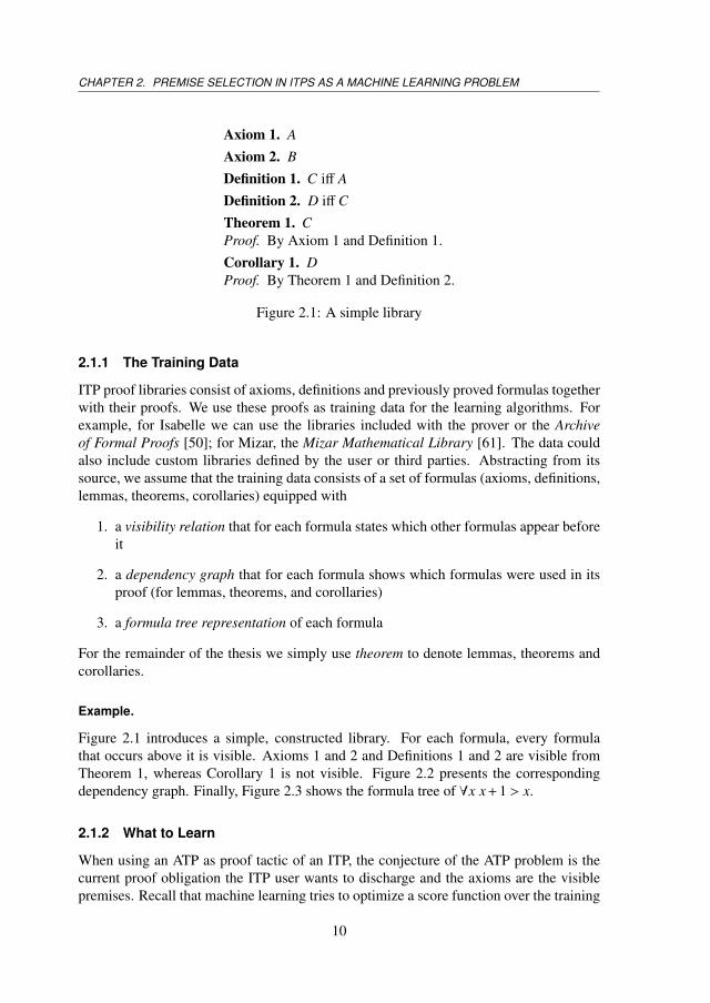
Theorem 1. CProof. By Axiom 1 and Definition 1.Corollary 1. DProof. By Theorem 1 and Definition 2.
Figure 2.1: A simple library
2.1.1 The Training Data
ITP proof libraries consist of axioms, definitions and previously proved formulas togetherwith their proofs. We use these proofs as training data for the learning algorithms. Forexample, for Isabelle we can use the libraries included with the prover or the Archiveof Formal Proofs [50]; for Mizar, the Mizar Mathematical Library [61]. The data couldalso include custom libraries defined by the user or third parties. Abstracting from itssource, we assume that the training data consists of a set of formulas (axioms, definitions,lemmas, theorems, corollaries) equipped with
1. a visibility relation that for each formula states which other formulas appear beforeit
2. a dependency graph that for each formula shows which formulas were used in itsproof (for lemmas, theorems, and corollaries)
3. a formula tree representation of each formula
For the remainder of the thesis we simply use theorem to denote lemmas, theorems andcorollaries.
Example.
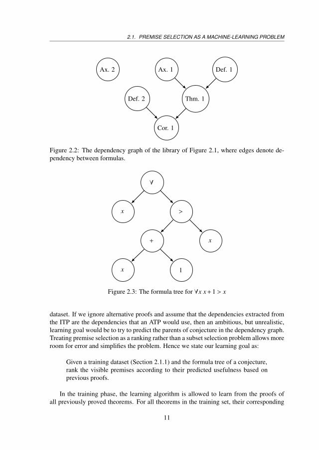
Figure 2.1 introduces a simple, constructed library. For each formula, every formulathat occurs above it is visible. Axioms 1 and 2 and Definitions 1 and 2 are visible fromTheorem 1, whereas Corollary 1 is not visible. Figure 2.2 presents the correspondingdependency graph. Finally, Figure 2.3 shows the formula tree of ∀x x + 1 > x.
2.1.2 What to Learn
When using an ATP as proof tactic of an ITP, the conjecture of the ATP problem is thecurrent proof obligation the ITP user wants to discharge and the axioms are the visiblepremises. Recall that machine learning tries to optimize a score function over the training
10
2.1. PREMISE SELECTION AS A MACHINE-LEARNING PROBLEM
Cor. 1
Thm. 1Def. 2
Ax. 1 Def. 1Ax. 2
Figure 2.2: The dependency graph of the library of Figure 2.1, where edges denote de-pendency between formulas.
∀
x >
+
x 1
x
Figure 2.3: The formula tree for ∀x x + 1 > x
dataset. If we ignore alternative proofs and assume that the dependencies extracted fromthe ITP are the dependencies that an ATP would use, then an ambitious, but unrealistic,learning goal would be to try to predict the parents of conjecture in the dependency graph.Treating premise selection as a ranking rather than a subset selection problem allows moreroom for error and simplifies the problem. Hence we state our learning goal as:
Given a training dataset (Section 2.1.1) and the formula tree of a conjecture,rank the visible premises according to their predicted usefulness based onprevious proofs.
In the training phase, the learning algorithm is allowed to learn from the proofs ofall previously proved theorems. For all theorems in the training set, their corresponding
11
CHAPTER 2. PREMISE SELECTION IN ITPS AS A MACHINE LEARNING PROBLEM
ATP problem i
ATP problem 1
ATP problem m
Premise ranking
Sledgehammer
n1highest ranked premises
ni highest ranked premises
nm highest ranked premises
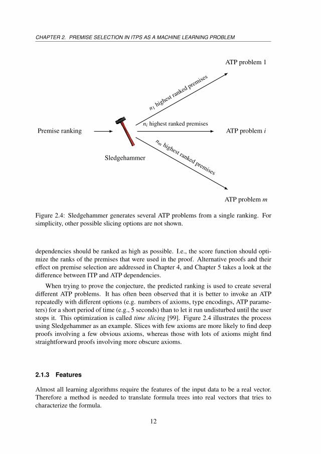
Figure 2.4: Sledgehammer generates several ATP problems from a single ranking. Forsimplicity, other possible slicing options are not shown.
dependencies should be ranked as high as possible. I.e., the score function should opti-mize the ranks of the premises that were used in the proof. Alternative proofs and theireffect on premise selection are addressed in Chapter 4, and Chapter 5 takes a look at thedifference between ITP and ATP dependencies.
When trying to prove the conjecture, the predicted ranking is used to create severaldifferent ATP problems. It has often been observed that it is better to invoke an ATPrepeatedly with different options (e.g. numbers of axioms, type encodings, ATP parame-ters) for a short period of time (e.g., 5 seconds) than to let it run undisturbed until the userstops it. This optimization is called time slicing [99]. Figure 2.4 illustrates the processusing Sledgehammer as an example. Slices with few axioms are more likely to find deepproofs involving a few obvious axioms, whereas those with lots of axioms might findstraightforward proofs involving more obscure axioms.
2.1.3 Features
Almost all learning algorithms require the features of the input data to be a real vector.Therefore a method is needed to translate formula trees into real vectors that tries tocharacterize the formula.
12
2.1. PREMISE SELECTION AS A MACHINE-LEARNING PROBLEM
Symbols.
The symbols that appear in a formula can be seen as its basic characterization and hence asimple approach is to take the set of symbols of a formula as its feature set. The symbolscorrespond to the node labels in the formula tree.
Let n ∈ N denote the vector size, which should be at least as large as the total numberof symbols in the library. Let i be an injective index function that maps each symbol sto a positive number i(s) ≤ n. The feature representation of a formula tree t is the binaryvector ϕ(t) such that ϕ(t)( j) = 1 iff the symbol with index j appears in t.
The example formula tree in Figure 2.3 contains the symbols ∀, >, +, x, and 1. Givenn = 10, i(∀) = 1, i(>) = 4, i(+) = 6, i(x) = 7, and i(1) = 8, the corresponding feature vectoris (1,0,0,1,0,1,1,1,0,0).
Subterms and subformulas.
In addition to the symbols, one can also include as features the subterms and subformulasof the formula to prove—i.e., the subtrees of the formula tree [110]. For example, the for-mula tree in Figure 2.3 has subtrees associated with x, 1, x+1, x > x+1, and ∀x x+1 > x.Adding all subtrees significantly increases the size of the feature vector. Many subtermsand subformulas appear only once in the library and are hence useless for making predic-tions. An approach to curtail this explosion is to consider only small subtrees (e.g., thosewith a height of at most 2 or 3).
Types.
The formalisms supported by the vast majority of ITP systems are typed (or sorted),meaning that each term can be given a type that describes the values that can be taken bythe term. Examples of types are int, real, real× real, and real→ real. Adding the typesthat appear in the formula tree as additional features is reasonable [56, 45]. Like terms,types can be represented as trees, and we may choose between encoding only basic typesor also some or all complex subtypes.
Context.
Due to the way humans develop complex proofs, the last few formulas that were provedare likely to be useful in a proof of the current goal [24]. However, the machine learningalgorithm might rank them poorly because they are new and hence little used, if at all.Adding the feature vectors of some of the last previously proved theorems to the featurevector of the conjecture, in a weighted fashion, is a way to add information about thecontext in which the conjecture occurs to the feature vector. This method is particularlyuseful when a formula has very few or very general features but occurs in a wider context.
13
CHAPTER 2. PREMISE SELECTION IN ITPS AS A MACHINE LEARNING PROBLEM
2.2 Naive Bayes and Kernel-Based Learning
We give a detailed example of an actual learning setup using a standard naive Bayes andthe kernel-based Multi-Output Ranking (MOR) algorithm. The mathematics underlyingboth algorithms are introduced and the benefits of kernels explained. Naive Bayes hasalready been used in previous work on premise selection [110] whereas the MOR algo-rithm is newly introduced in this thesis. The next chapter contains an evaluation of thesetwo (among other) algorithms.
2.2.1 Formal Setting
Let Γ be the set of formulas that appear in the training dataset.
Definition 1 (Proof matrix). For two formulas c, p ∈ Γ we define the proof matrix µ :Γ×Γ→ {0,1} by
µ(c, p)B
1 if p is used to prove c,0 otherwise.
In other words, µ is the adjacency matrix of the dependency graph.
The used premises of a formulas c are the direct parents of c in the dependency graph.
usedPremises(c)B {p | µ(c, p) = 1}
Definition 2 (Feature matrix). Let T B {t1, . . . , tm} be a fixed enumeration of the set of allsymbols and (sub)terms that appear in all formulas from Γ.2 We define Φ : Γ×{1, . . . ,m}→{0,1} by
Φ(c, i)B
1 if ti appears in c,0 otherwise.
This matrix gives rise to the feature function ϕ : Γ→ {0,1}m which for c ∈ Γ is the vectorϕc with entries in {0,1} satisfying
ϕci = 1 ⇐⇒ Φ(c, i) = 1.
The expressed features of a formula are denoted by the value of the function e : Γ→P(T )that maps c to {ti | Φ(c, i) = 1}.
For each premise p ∈ Γ we learn a real-valued classifier function Cp(·) : Γ→ R which,given a conjecture c, estimates how useful p is for proving c. The premises for a con-jecture c ∈ Γ are ranked by the values of Cp(c). The main difference between learningalgorithms is the function space in which they search for the classifiers and the measurethey use to evaluate how good a classifier is.
2If the set of features is not constant they are enumerated in order of appearance.
14
2.2. NAIVE BAYES AND KERNEL-BASED LEARNING
2.2.2 A Naive Bayes Classifier
Naive Bayes is a statistical learning method based on Bayes’ theorem about conditionalprobabilities3 with a strong (read: naive) independence assumptions. In the naive Bayessetting, the value Cp(c) of the classifier function of a premise p at a conjecture c is theprobability that µ(c, p) = 1 given the expressed features e(c).
To understand the difference between the naive Bayes and the kernel-based learningalgorithm we need to take a closer look at the naive Bayes classifier. Let θ denote thestatement that µ(c, p) = 1 and for each feature ti ∈ T let ti denote that Φ(c, i) = 1. Fur-thermore, let e(c) = {s1, . . . , sl} ⊆ T be the expressed features of c (with correspondings1, . . . , sl). Then (by Bayes’ theorem) we have
P(θ | s1, . . . , sl) ∝ P(s1, . . . , sl | θ)P(θ) (2.1)
where the logarithm of the right-hand side can be computed as
ln P(s1, . . . , sl | θ)P(θ) = ln P(s1, . . . , sl | θ) + ln P(θ) (2.2)
= lnl∏
i=1
P(si | θ) + ln P(θ) by independence (2.3)
=
m∑i=1
ϕci ln P(ti | θ) + ln P(θ) (2.4)
= wTϕc + ln P(θ) (2.5)
wherewi B ln P(ti | θ) (2.6)
There are two things worth noting here. First, P(ti | θ) and P(θ) might be 0. In thatcase, taking the natural logarithm would not be defined. In practice, if P(ti | θ) or P(θ)are 0 the algorithm replaces the 0 with a predefined very small ε > 0. Second, line (5)shows that the naive-Bayes classifier is “essentially” (after the monotonic transformation)a linear function of the features of the conjecture. The feature weights w are computedusing formula (2.6).
2.2.3 Kernel-based Learning
We saw that the naive Bayes algorithm gives rise to a linear classifier. This leads toseveral questions: ‘Are there better weights?’ and ‘Can one get better performance withnon-linear functions?’. Kernel-based learning provides a framework for investigatingsuch questions. In this subsection we give a simplified, brief description of kernel-basedlearning that is tailored to our present problem; further information can be found in [5,82, 88].
3In its simplest form, Bayes’ theorem asserts for a probability function P and random variables X and Ythat
P(X|Y) =P(Y |X)P(X)
P(Y),
where P(X|Y) is understood as the conditional probability of X given Y .
15
CHAPTER 2. PREMISE SELECTION IN ITPS AS A MACHINE LEARNING PROBLEM
Are there better weights?
To answer this question we must first define what ‘better’ means. Using the number ofproblems solved as measure is not feasible because we cannot practically run an ATP forevery possible weight combination. Instead, we measure how good a classifier approxi-mates our training data. We would like to have that
∀x ∈ Γ : Cp(x) = µ(x, p).
However, this will almost never be the case. To compare how well a classifier approxi-mates the data, we use loss functions and the notion of expected loss that they provide,which we now define.
Definition 3 (Loss function and Expected Loss). A loss function is any function l : R×R→ R+. Given a loss function l we can then define the expected loss E(·) of a classifierCp as
E(Cp) =∑x∈Γ
l(Cp(x),µ(x, p))
One might add additional properties such as l(x, x) = 0, but this is not necessary. Typ-ical examples of a loss function l(x,y) are the square loss (y− x)2 or the 0-1 loss definedby I(x = y).4
We can compare two different classifiers via their expected loss. If the expected loss ofclassifier Cp is less than the expected loss of a classifier C′p then Cp is the better classifier.
Nonlinear Classifiers
It seems straightforward that more complex functions would lead to a lower expected lossand are hence desirable. However, weight optimization becomes tedious once we leavethe linear case. Kernels provide a way to use the machinery of linear optimization onnon-linear functions.
Definition 4 (Kernel). A kernel is is a function k : Γ×Γ→ R satisfying
k(x,y) = 〈φ(x),φ(y)〉
where φ : Γ→ F is a mapping from Γ to an inner product space F with inner product 〈·, ·〉.A kernel can be understood as a similarity measure between two entities.
Example 1. A standard example is the linear kernel:
klin(x,y)B 〈ϕx,ϕy〉
with 〈·, ·〉 being the normal dot product in Rm. Here, ϕ f denotes the features of a formulaf , and the inner product space F is Rm. A nontrivial example is the Gaussian kernel withparameter σ [13]:
kgauss(x,y)B exp(−〈ϕx,ϕx〉−2〈ϕx,ϕy〉+ 〈ϕy,ϕy〉
σ2
)4I is defined as follows: I(x = y) = 0 if x = y, and I(x = y) = 1 otherwise.
16
2.2. NAIVE BAYES AND KERNEL-BASED LEARNING
We can now define our kernel function space in which we will search for classificationfunctions.
Definition 5 (Kernel Function Space). Given a kernel k, we define
Fk B
f ∈ RΓ | f (x) =∑v∈Γ
αvk(x,v),αv ∈ R,‖ f ‖ <∞
.as our kernel function space, where for f (x) =
∑v∈Γαvk(x,v)
‖ f ‖ =∑u,v∈Γ
αuαvk(u,v)
Essentially, every function in Fk compares the input x with formulas in Γ using the kernel,and the weights α determine how important each comparison is.5
The kernel function space Fk naturally depends on the kernel k. It can be shown thatwhen we use klin, Fklin consists of linear functions of the features T . In contrast, theGaussian kernel kgauss gives rise to a nonlinear (in the features) function space.
Putting it all together
Having defined loss functions, kernels and kernel function spaces we can now definehow kernel-based learning algorithms learn classifier functions. Given a kernel k and aloss function l, recall that we measure how good a classifier Cp is with the expected lossE(Cp). With all our definitions it seems reasonable to define Cp as
Cp B argminf∈Fk
E( f ) (2.7)
However, this is not what a kernel based learning algorithm does. There are two reasonsfor this. First, the minimum might not exist. Second, in particular when using complexkernel functions, such an approach might lead to overfitting: Cp might perform very wellon our training data, but badly on data that was not seen before. To handle both problems,a regularization parameter λ > 0 is introduced to penalize complex functions. This regu-larization parameter allows us to place a bound on possible solution which together withthe fact that Fk is a Hilbert space ensures the existence of Cp. Hence we define
Cp = argminf∈Fk
E( f ) +λ‖ f ‖2 (2.8)
Recall from the definition of Fk that Cp has the form
Cp(x) =∑v∈Γ
αvk(x,v), (2.9)
with αv ∈ R. Hence, for any fixed λ, we only need to compute the weights αv for all v ∈ Γ
in order to define Cp. In Section 2.2.4 we show how to solve this optimization problemin our setting.
5Schölkopf gives a more general approach to kernel spaces [81].
17
CHAPTER 2. PREMISE SELECTION IN ITPS AS A MACHINE LEARNING PROBLEM
Naive Bayes vs Kernel-based Learning
Kernel-based methods typically outperform the naive Bayes algorithm. There are severalreasons for this. Firstly and most importantly, while naive Bayes is essentially a linearclassifier, kernel based methods can learn non-linear dependencies when an appropriatenon-linear (e.g. Gaussian) kernel function is used. This advantage in expressivenessusually leads to significantly better generalization6 performance of the algorithm givenproperly estimated hyperparameters (e.g., the kernel width σ for Gaussian functions).Secondly, kernel-based methods are formulated within the regularization framework thatprovides mechanism to control the errors on the training set and the complexity ("expres-siveness") of the prediction function. Such setting prevents overfitting of the algorithmand leads to notably better results compared to unregularized methods. Thirdly, some ofthe kernel-based methods (depending on the loss function) can use very efficient proce-dures for hyperparameter estimation (e.g. fast leave-one-out cross-validation [78]) andtherefore result in a close to optimal model for the classification/regression task. For suchreasons kernel-based methods are among the most successful algorithms applied to var-ious problems from bioinformatics to information retrieval to computer vision [88]. Ageneral advantage of naive Bayes over kernel-based algorithms is the computational effi-ciency, particularly when taking into account the fact that computing the kernel matrix isgenerally quadratic in the number of training data points.
2.2.4 Multi-Output Ranking
We define the kernel-based multi-output ranking (MOR) algorithm. It extends previouslydefined preference learning algorithms by Tsivtsivadze and Rifkin [100, 78]. Let Γ =
{x1, . . . , xn}. Then formula (2.9) becomes
Cp(x) =
n∑i=1
αik(x, xi)
Using this and the square-loss l(x,y) = (x− y)2 function, solving equation (2.8) is equiva-lent to finding weights αi that minimize
minα1,...,αn
n∑i=1
n∑j=1
α jk(xi, x j)−µ(xi, p)
2
+λ
n∑i, j=1
αiα jk(xi, x j)
(2.10)
Recall that Cp is the classifier for a single premise. Since we eventually want to rankall premises, we need to train a classifier for each premise. So we need to find weightsαi,p for each premise p. We can use the fact that for each premise p, Cp depends on thevalues of k(xi, x j), where 1 ≤ i, j ≤ n, to speed up the computation. Instead of learning theclassifiers Cp for each premise separately, we learn all the weights αp,i simultaneously.
6Generalization is the ability of a machine learning algorithm to perform accurately on new, unseen exam-ples after training on a finite data set.
18
2.3. CHALLENGES
To do this, we first need some definitions. Let
A = (αi,p)i,p (1 ≤ i ≤ n, p ∈ Γ).
A is the matrix where each column contains the parameters of one premise classifier.Define the kernel matrix K and the label matrix Y as
K B (k(xi, x j))i, j (1 ≤ i, j ≤ n)Y B (µ(xi, p))i,p (1 ≤ i ≤ n, p ∈ Γ).
We can now rewrite (2.10) in matrix notation to state the problem for all premises:
argminA
tr((Y −KA)T(Y −KA) +λATKA
)(2.11)
where tr(A) denotes the trace of the matrix A. Taking the derivative with respect to Aleads to:
∂∂A tr
((Y −KA)T(Y −KA) +λATKA
)= tr (−2K(Y −KA) + 2λKA)
= tr (−2KY + (2KK + 2λK)A)
To find the minimum, we set the derivative to zero and solve with respect to A. This leadsto:
A = (K +λI)−1Y (2.12)
If the regularization parameter λ and the (potential) kernel parameter σ are fixed, wecan find the optimal weights through simple matrix computations. Thus, to fully deter-mine the classifiers, it remains to find good values for the parameters λ and σ. This isdone, as is common with such parameter optimization for kernel methods, by simple (log-arithmically scaled) grid search and cross-validation on the training data using a 70/30split. For this, we first define a logarithmically scaled set of potential parameters. Thetraining set in then randomly split in two parts cvtrain and cvtest with cvtrain containing70% of the training data and cvtest containing the remaining 30%. For each set of param-eters, the algorithm is trained on cvtrain and evaluated on cvtest. The process is repeated10 times. The set of parameters with the best average performance is then picked for thereal evaluation.
2.3 Challenges
Premise selection has several peculiarities that restrict which machine learning algorithmscan be effectively used. In this section, we illustrate these challenges on a large fragmentof Isabelle’s Archive of Formal Proofs (AFP). The AFP benchmarks contain 165964 for-mulas distributed over 116 entries contributed by dozens of Isabelle users.7 Most entriesare related to computer science (e.g., data structures, algorithms, programming languages,and process algebras). The dataset was generated using Sledgehammer [56] and is avail-able publicly at http://www.cs.ru.nl/~kuehlwein/downloads/afp.tar.gz.
7A number of AFP entries were omitted because of technical difficulties.
19
CHAPTER 2. PREMISE SELECTION IN ITPS AS A MACHINE LEARNING PROBLEM
2.3.1 Features
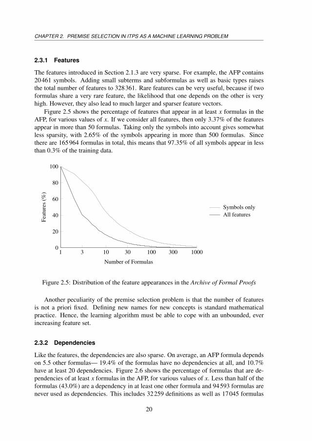
The features introduced in Section 2.1.3 are very sparse. For example, the AFP contains20461 symbols. Adding small subterms and subformulas as well as basic types raisesthe total number of features to 328361. Rare features can be very useful, because if twoformulas share a very rare feature, the likelihood that one depends on the other is veryhigh. However, they also lead to much larger and sparser feature vectors.
Figure 2.5 shows the percentage of features that appear in at least x formulas in theAFP, for various values of x. If we consider all features, then only 3.37% of the featuresappear in more than 50 formulas. Taking only the symbols into account gives somewhatless sparsity, with 2.65% of the symbols appearing in more than 500 formulas. Sincethere are 165964 formulas in total, this means that 97.35% of all symbols appear in lessthan 0.3% of the training data.
1 3 10 30 100 300 10000
20
40
60
80
100
Number of Formulas
Feat
ures
(%)
Symbols onlyAll features
Figure 2.5: Distribution of the feature appearances in the Archive of Formal Proofs
Another peculiarity of the premise selection problem is that the number of featuresis not a priori fixed. Defining new names for new concepts is standard mathematicalpractice. Hence, the learning algorithm must be able to cope with an unbounded, everincreasing feature set.
2.3.2 Dependencies
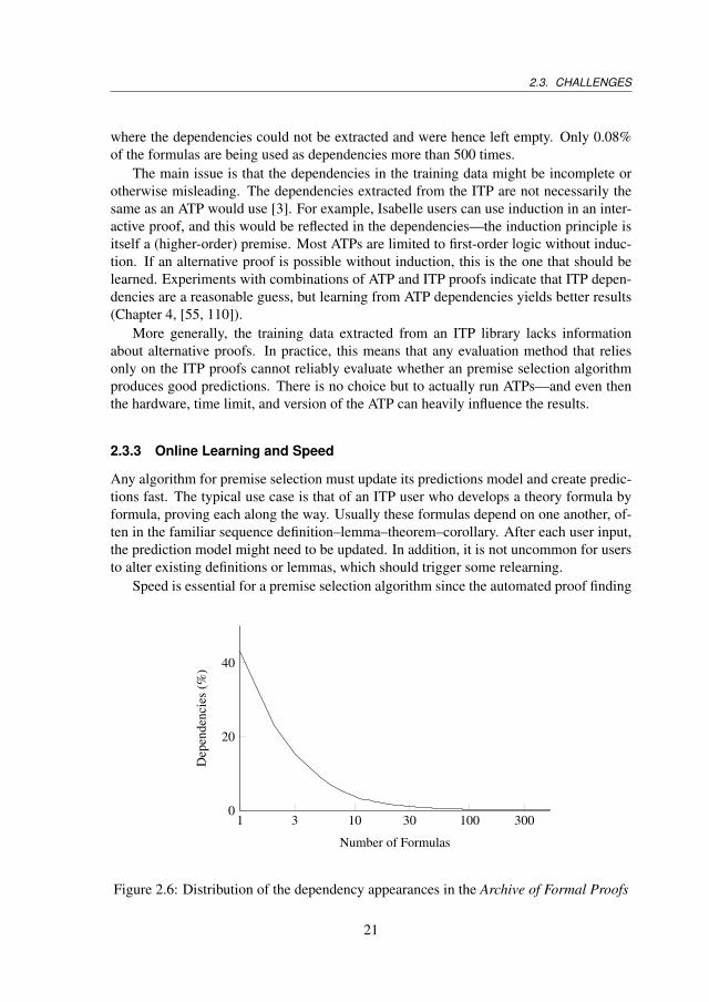
Like the features, the dependencies are also sparse. On average, an AFP formula dependson 5.5 other formulas— 19.4% of the formulas have no dependencies at all, and 10.7%have at least 20 dependencies. Figure 2.6 shows the percentage of formulas that are de-pendencies of at least x formulas in the AFP, for various values of x. Less than half of theformulas (43.0%) are a dependency in at least one other formula and 94593 formulas arenever used as dependencies. This includes 32259 definitions as well as 17045 formulas
20
2.3. CHALLENGES
where the dependencies could not be extracted and were hence left empty. Only 0.08%of the formulas are being used as dependencies more than 500 times.
The main issue is that the dependencies in the training data might be incomplete orotherwise misleading. The dependencies extracted from the ITP are not necessarily thesame as an ATP would use [3]. For example, Isabelle users can use induction in an inter-active proof, and this would be reflected in the dependencies—the induction principle isitself a (higher-order) premise. Most ATPs are limited to first-order logic without induc-tion. If an alternative proof is possible without induction, this is the one that should belearned. Experiments with combinations of ATP and ITP proofs indicate that ITP depen-dencies are a reasonable guess, but learning from ATP dependencies yields better results(Chapter 4, [55, 110]).
More generally, the training data extracted from an ITP library lacks informationabout alternative proofs. In practice, this means that any evaluation method that reliesonly on the ITP proofs cannot reliably evaluate whether an premise selection algorithmproduces good predictions. There is no choice but to actually run ATPs—and even thenthe hardware, time limit, and version of the ATP can heavily influence the results.
2.3.3 Online Learning and Speed
Any algorithm for premise selection must update its predictions model and create predic-tions fast. The typical use case is that of an ITP user who develops a theory formula byformula, proving each along the way. Usually these formulas depend on one another, of-ten in the familiar sequence definition–lemma–theorem–corollary. After each user input,the prediction model might need to be updated. In addition, it is not uncommon for usersto alter existing definitions or lemmas, which should trigger some relearning.
Speed is essential for a premise selection algorithm since the automated proof finding
1 3 10 30 100 3000
20
40
Number of Formulas
Dep
ende
ncie
s(%
)
Figure 2.6: Distribution of the dependency appearances in the Archive of Formal Proofs
21
CHAPTER 2. PREMISE SELECTION IN ITPS AS A MACHINE LEARNING PROBLEM
process needs to be faster than manual proof creation. The less time is spent on updatingthe learning model and predicting the premise ranking, the more time can be used byATPs. Users of ITPs tend to be impatient: If the automated provers do not respond withinhalf a minute or so, they usually prefer to carry out the proof themselves.
22
Chapter 3
Overview and Evaluation of PremiseSelection Techniques
In this chapter, an overview of state-of-the-art techniques for premise selection in largetheory mathematics is presented, and new premise selection techniques are introduced.Several evaluation metrics are defined and their appropriateness is discussed in the con-text of automated reasoning in large theory mathematics. The methods are evaluatedon the MPTP2078 benchmark, a subset of the Mizar library, and a 10% improvement isobtained over the best method so far.
3.1 Premise Selection Algorithms
3.1.1 Premise Selection Setting
The typical setting for the task of premise selection is a large developed library of for-mally encoded mathematical knowledge, over which mathematicians attempt to provenew lemmas and theorems[102, 15, 109]. The actual mathematical corpora suitable forATP techniques are only a fraction of all mathematics (e.g. about 52000 lemmas andtheorems in the Mizar library) and started to appear only recently, but they already pro-vide a corpus on which different methods can be defined, trained, and evaluated. Premiseselection can be useful as a standalone service for the formalizers (suggesting relevantlemmas), or in conjunction with ATP methods that can attempt to find a proof from therelevant premises.
This chapter is based on: [57] “Overview and Evaluation of Premise Selection Techniques for LargeTheory Mathematics”, published in the Proceedings of the 6th International Joint Conference on AutomatedReasoning.
23
CHAPTER 3. OVERVIEW OF PREMISE SELECTION TECHNIQUES
3.1.2 Learning-based Ranking Algorithms
Learning-based ranking algorithms have a training and a testing phase and typically rep-resent the data as points in pre-selected feature spaces. In the training phase the algorithmtries to fit one (or several) prediction functions to the data it is given. The result of thetraining is the best fitting prediction function which can then be used in the testing phasefor evaluations.
In the typical setting presented above, the algorithms would train on all existing proofsin the library and be tested on the new theorem the mathematician wants to prove. Wecompare three different algorithms.
SNoW: SNoW (Sparse Network of Winnows)[21] is an implementation of (among oth-ers) the naive Bayes algorithm that has already been successfully used for premise selec-tion [102, 105, 2].
Naive Bayes is a statistical learning method based on Bayes‘ theorem with a strong(or naive) independence assumption. Given a new conjecture c and a premise p, SNoWcomputes the probability of p being needed to prove c, based on the previous use of p inproving conjectures that are similar to c. The similarity is in our case typically expressedusing symbols and terms of the formulas. The independence assumption says that the(non-)occurrence of a symbol/term is not related to the (non-)occurrence of every othersymbol/term. A detailed description can be found in Section 2.2.4.
MOR-CG: MOR-CG (Multi-Output Ranking with Conjugate Gradient) is a kernel-basedlearning algorithm [88] that is a faster version of the MOR algorithm described the pre-vious Chapter. Instead of doing an exact computation of the weights as presented inSection 2.2.4, MOR-CG uses conjugate-gradient descent [89] which speeds up the timeneeded for training. Since preliminary tests gave the best results for a linear kernel, thefollowing experiments are based on a linear kernel.
Kernel-based algorithms do not aim to model probabilities, but instead try to minimizethe expected loss of the prediction functions on the training data. For each premise pMOR-CG tries to find a function Cp such that for each conjecture c, Cp(c) = 1 iff p wasused in the proof of c. Given a new conjecture c, we can evaluate the learned predictionfunctions Cp on c. The higher the value Cp(c) the more relevant p is to prove c.
BiLi: BiLi (Bi-Linear) is a new algorithm by Twan van Laarhoven that is based on abilinear model of premise selection, similar to the work of Chu and Park [23]. Like MOR-CG, BiLi aims to minimize the expected loss. The difference lies in the kind of predictionfunctions they produce. In MOR-CG the prediction functions only take the features1 ofthe conjecture into account. In BiLi, the prediction functions use the features of boththe conjectures and the premises. This makes BiLi a similar to methods like SInE thatsymbolically compare conjectures with premises. The bilinear model learns a weight for
1In our experiments each feature indicates the presence or absence of a certain symbol or term in a formula.
24
3.1. PREMISE SELECTION ALGORITHMS
each combination of a conjecture feature together with a premise feature. Together, thisweighted combination determines whether or not a premise is relevant to the conjecture.
When the number of features becomes large, fitting a bilinear model becomes com-putationally more challenging. Therefore, in BiLi the number of features is first reducedto 100, using random projections [12]. To combat the noise introduced by these randomprojections, this procedure is repeated 20 times, and the averaged predictions are used forranking the premises.
3.1.3 Other Algorithms Used in the Evaluation
SInE: SInE, the SUMO Inference Engine, is a heuristic state-of-the-art premise selectionalgorithm by Kryštof Hoder [41]. The basic idea is to use global frequencies of symbolsin a problem to define their generality, and build a relation linking each symbol S withall formulas F in which S is has the lowest global generality among the symbols of F.In common-sense ontologies, such formulas typically define the symbols linked to them,which is the reason for calling this relation a D-relation. Premise selection for a conjec-ture is then done by recursively following the D-relation, starting with the conjecture’ssymbols.
For the experiments described here the E implementation2 of SInE has been used, be-cause it can be instructed to select exactly the N most relevant premises. This is compat-ible with the way other premise rankers are used in this chapter, and it allows to comparethe premise rankings produced by different algorithms for increasing values of N.3
Aprils: APRILS [79], the Automated Prophesier of Relevance Incorporating Latent Se-mantics, is a signature-based premise selection method that employs Latent SemanticAnalysis (LSA) [26] to define symbol and premise similarity. Latent semantics is a ma-chine learning method that has been successfully used for example in the Netflix Prize,4
and in web search. Its principle is to automatically derive “semantic” equivalence classesof words (like car, vehicle, automobile) from their co-occurrences in documents, and towork with such equivalence classes instead of the original words. In APRILS, formulasdefine the symbol co-occurrence, each formula is characterized as a vector over the sym-bols’ equivalence classes, and the premise relevance is its dot product with the conjecture.
3.1.4 Techniques Not Included in the Evaluation
As a part of the overview, we also list important or interesting algorithms used for ATPknowledge selection that for various reasons do not fit this the evaluation. We refer readersto [106] for their discussion.
2http://www.mpi-inf.mpg.de/departments/rg1/conferences/deduction10/slides/stephan-schulz.pdf
3The exact parameters used for producing the E-SInE rankings are athttps://raw.github.com/JUrban/MPTP2/master/MaLARea/script/filter1.
4http://www.netflixprize.com
25
CHAPTER 3. OVERVIEW OF PREMISE SELECTION TECHNIQUES
• The default premise selection heuristic used by the Isabelle/Sledgehammer ex-port [64]. This is an Isabelle-specific symbol-based technique similar to SInE thatwould need to be evaluated on Isabelle data.• Goal directed ATP calculi including the Conjecture Symbol Weight clause selection
heuristics in E prover [84] giving lower weights to symbols contained in the con-jecture, the Set of Support (SoS) strategy in resolution/superposition provers, andtableau calculi like leanCoP [70] that are in practice goal-oriented.• Model-based premise selection, as done by Pudlák’s semantic axiom selection sys-
tem for large theories [76], by the SRASS metasystem [97], and in a different set-ting by the MaLARea [110] metasystem.• MaLARea [110] is a large-theory metasystem that loops between deductive proof
and model finding (using ATPs and finite model finders), and learning premise-selection (currently using SNoW or MOR-CG) from the proofs and models to at-tack the conjectures that still remain to be proved.• Abstract proof trace guidance implemented in the E prover by Stephan Schulz for
his PhD [83]. Proofs are abstracted into clause patterns collected into a commonknowledge base, which is loaded when a new problem is solved, and used for guid-ing clause selection. This is also similar to the hints technique in Prover9 [63].• The MaLeCoP system [112] where the clause relevance is learned from all closed
tableau branches, and the tableau extension steps are guided by a trained machinelearner that takes as input features a suitable encoding of the literals on the currenttableau branch.
3.2 Machine Learning Evaluation Metrics
Given a database of proofs, there are several possible ways to evaluate how good a premiseselection algorithm is without running an ATP. Such evaluation metrics are used to esti-mate the best parameters (e.g. regularization, tolerance, step size) of an algorithm. Theinput for each metric is a ranking of the premises for a conjecture together with the in-formation which premises where used to prove the conjecture (according to the trainingdata).
Recall
Recall@n is a value between 0 and 1 and denotes the fraction of used premises that areamong the top n highest ranked premises.
Recall@n =
∣∣∣{used premises}∩ {n highest ranked premises}∣∣∣∣∣∣{used premises}
∣∣∣Recall@n is always less than Recall@(n + 1). As n increases, Recall@n will eventu-ally converge to 1. Our intuition is that the better the algorithm, the faster its Recall@nconverges to 1.
26
3.3. EVALUATION
AUC
The AUC (Area under the ROC Curve) is the probability that, given a randomly drawnused premise and a randomly drawn unused premise, the used premise is ranked higherthan the unused premise. Values closer to 1 show better performance.
Let x1, .., xn be the ranks of the used premises and y1, ..,ym be the ranks of the unusedpremises. Then, the AUC is defined as
AUC =
∑ni∑m
j 1xi>y j
mn
where 1xi>y j = 1 iff xi > y j and zero otherwise.
100%Recall
100%Recall denotes the minimum n such that Recall@n = 1.
100%Recall = min{n | Recall@n = 1}
In other words 100%Recall tells us how many premises (starting from the highest rankedone) we need to give to the ATP to ensure that all necessary premises are included.
3.3 Evaluation
3.3.1 Evaluation Data
The premise selection methods are evaluated on the large (chainy) problems from theMPTP2078 benchmark5.[2] These are 2078 related large-theory problems (conjectures)and 4494 formulas (conjectures and premises) in total, extracted from the Mizar Math-ematical Library (MML). The MPTP2078 benchmark was developed to supersede theolder and smaller MPTP Challenge benchmark (developed in 2006), while keeping thenumber of problems manageable for experimenting. Larger evaluations are possible,6
but not convenient when testing a large number of systems with many different settings.MPTP2078 seems sufficiently large to test various hypotheses and find significant differ-ences.
MPTP2078 also contains (in the smaller, bushy problems) for each conjecture theinformation about the premises used in the MML proof. This can be used to train andevaluate machine learning algorithms using a chronological order emulating the growthof MML. For each conjecture, the algorithms are allowed to train on all MML proofs thatwere done up to (not including) the current conjecture. For each of the 2078 problems,the algorithms predict a ranking of the premises.
5Available at http://wiki.mizar.org/twiki/bin/view/Mizar/MpTP2078.6See [108, 3] for recent evaluations spanning the whole MML.
27
CHAPTER 3. OVERVIEW OF PREMISE SELECTION TECHNIQUES
3.3.2 Machine Learning Evaluation: Comparison of Predictions with KnownProofs
We first compare the algorithms introduced in section 3.1 using the machine learningevaluation metrics introduced in section 3.2. All evaluations are based on the trainingdata, the human-written formal proofs from the MML. They do not take alternative proofsinto account.
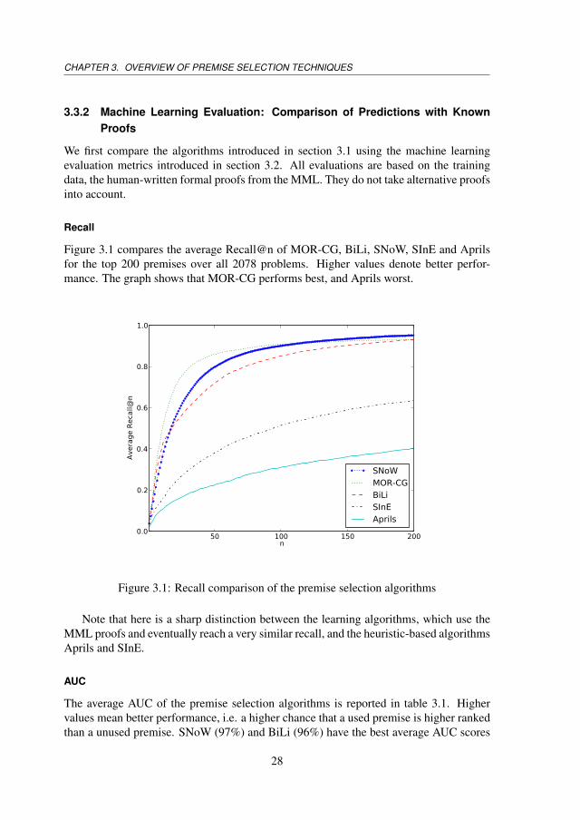
Recall
Figure 3.1 compares the average Recall@n of MOR-CG, BiLi, SNoW, SInE and Aprilsfor the top 200 premises over all 2078 problems. Higher values denote better perfor-mance. The graph shows that MOR-CG performs best, and Aprils worst.
50 100 150 200n
0.0
0.2
0.4
0.6
0.8
1.0
Aver
age
Reca
ll@n
SNoWMOR-CGBiLiSInEAprils
Figure 3.1: Recall comparison of the premise selection algorithms
Note that here is a sharp distinction between the learning algorithms, which use theMML proofs and eventually reach a very similar recall, and the heuristic-based algorithmsAprils and SInE.
AUC
The average AUC of the premise selection algorithms is reported in table 3.1. Highervalues mean better performance, i.e. a higher chance that a used premise is higher rankedthan a unused premise. SNoW (97%) and BiLi (96%) have the best average AUC scores
28
3.3. EVALUATION
with MOR-CG taking the third spot with an average AUC of 88%. Aprils and SInE areconsiderably worse with 64% and 42% respectively. The standard deviation is very lowwith around 2% for all algorithms.
Table 3.1: AUC comparison of the premise selection algorithms
Algorithm Avg. AUC Std.
SNoW 0.9713 0.0216BiLi 0.9615 0.0215MOR-CG 0.8806 0.0206Aprils 0.6443 0.0176SInE 0.4212 0.0142
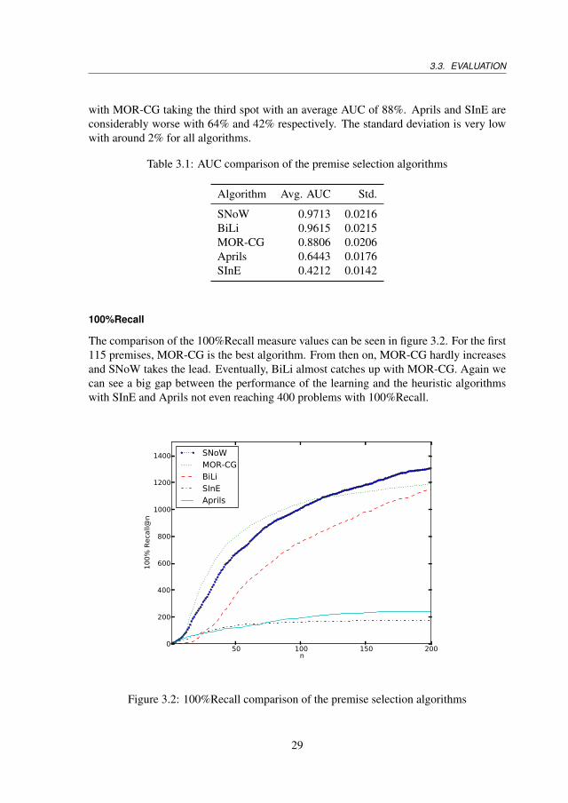
100%Recall
The comparison of the 100%Recall measure values can be seen in figure 3.2. For the first115 premises, MOR-CG is the best algorithm. From then on, MOR-CG hardly increasesand SNoW takes the lead. Eventually, BiLi almost catches up with MOR-CG. Again wecan see a big gap between the performance of the learning and the heuristic algorithmswith SInE and Aprils not even reaching 400 problems with 100%Recall.
50 100 150 200n
0
200
400
600
800
1000
1200
1400
100%
Rec
all@
n
SNoWMOR-CGBiLiSInEAprils
Figure 3.2: 100%Recall comparison of the premise selection algorithms
29
CHAPTER 3. OVERVIEW OF PREMISE SELECTION TECHNIQUES
Discussion
In all three evaluation metrics there is a clear difference between the performance of thelearning-based algorithms SNoW, MOR-CG and BiLi and the heuristic-based algorithmsSInE and Aprils. If the machine-learning metrics on the MML proofs are a good indicatorfor the ATP performance then there should be a corresponding performance difference inthe number of problems solved. We investigate this in the following section.
3.3.3 ATP Evaluation
Vampire
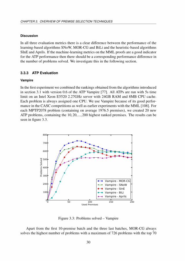
In the first experiment we combined the rankings obtained from the algorithms introducedin section 3.1 with version 0.6 of the ATP Vampire [77]. All ATPs are run with 5s timelimit on an Intel Xeon E5520 2.27GHz server with 24GB RAM and 8MB CPU cache.Each problem is always assigned one CPU. We use Vampire because of its good perfor-mance in the CASC competitions as well as earlier experiments with the MML [108]. Foreach MPTP2078 problem (containing on average 1976.5 premises), we created 20 newATP problems, containing the 10,20, ...,200 highest ranked premises. The results can beseen in figure 3.3.
0 50 100 150 200Used Premises
0
100
200
300
400
500
600
700
800
Prob
lem
s So
lved
Vampire - MOR-CGVampire - SNoWVampire - SInEVampire - BiLiVampire - Aprils
Figure 3.3: Problems solved – Vampire
Apart from the first 10-premise batch and the three last batches, MOR-CG alwayssolves the highest number of problems with a maximum of 726 problems with the top 70
30
3.3. EVALUATION
premises. SNoW solves less problems in the beginning, but catches up in the end. BiLisolves very few problems in the beginning, but gets better as more premises are given andeventually is as good as SNoW and MOR-CG. The surprising fact (given the machinelearning performance) is that SInE performs very well, on par with SNoW in the rangeof 60-100 premises. This indicates that SInE finds proofs that are very different from thehuman proofs. Furthermore, it is worth noting that most algorithms have their peak ataround 70-80 premises. It seems that after that, the effect of increased premise recall isbeaten by the effect of the growing ATP search space.
0 50 100 150 200Used Premises
0
100
200
300
400
500
600
700
800
Prob
lem
s So
lved
E - MOR-CGE - SNoWE - SInE
Figure 3.4: Problems solved – E
E, SPASS and Z3
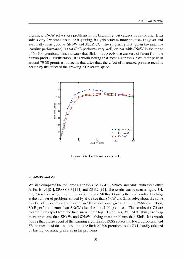
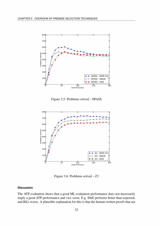
We also compared the top three algorithms, MOR-CG, SNoW and SInE, with three otherATPs: E 1.4 [84], SPASS 3.7 [114] and Z3 3.2 [66]. The results can be seen in figure 3.4,3.5, 3.6 respectively. In all three experiments, MOR-CG gives the best results. Lookingat the number of problems solved by E we see that SNoW and SInE solve about the samenumber of problems when more than 50 premises are given. In the SPASS evaluation,SInE performs better than SNoW after the initial 60 premises. The results for Z3 areclearer, with (apart from the first run with the top 10 premises) MOR-CG always solvingmore problems than SNoW, and SNoW solving more problems than SInE. It is worthnoting that independent of the learning algorithm, SPASS solves the fewest problems andZ3 the most, and that (at least up to the limit of 200 premises used) Z3 is hardly affectedby having too many premises in the problems.
31
CHAPTER 3. OVERVIEW OF PREMISE SELECTION TECHNIQUES
0 50 100 150 200Used Premises
0
100
200
300
400
500
600
700
800
Prob
lem
s So
lved
SPASS - MOR-CGSPASS - SNoWSPASS - SInE
Figure 3.5: Problems solved – SPASS
0 50 100 150 200Used Premises
0
100
200
300
400
500
600
700
800
Prob
lem
s So
lved
Z3 - MOR-CGZ3 - SNoWZ3 - SInE
Figure 3.6: Problems solved – Z3
Discussion
The ATP evaluation shows that a good ML evaluation performance does not necessarilyimply a good ATP performance and vice versa. E.g. SInE performs better than expected,and BiLi worse. A plausible explanation for this is that the human-written proofs that are
32
3.4. COMBINING PREMISE RANKERS
the basis of the learning algorithms are not the best possible guidelines for ATP proofs,because there are a number of good alternative proofs: the total number of problemsproved with Vampire by the union of all prediction methods is 1197, which is more (in5s) than the 1105 problems that Vampire can prove in 10s when using only the premisesused exactly in the human-written proofs. One possible way how to test this hypothesis(to a certain extent at least) would be to train the learning algorithms on all the ATP proofsthat are found, and test whether the ML evaluation performance closer correlates with theATP evaluation performance.
The most successful 10s combination, solving 939 problems, is to run Z3 with the 130best premises selected by MOR-CG, together with Vampire using the 70 best premises se-lected by SInE. It is also worth noting that when we consider all provers and all methods,1415 problems can be solved.
It seems the heuristic and the learning based premise selection methods give rise todifferent proofs. In the next section, we try to exploit this by considering combinations ofranking algorithms.
3.4 Combining Premise Rankers
There is clear evidence about alternative proofs being feasible from alternative predic-tions. This should not be too surprising, because the premises are organized into alarge derivation graph, and there are many explicit (and also quite likely many yet-undiscovered) semantic dependencies among them.
The evaluated premise selection algorithms are based on different ideas of similarity,relevance, and functional approximation spaces and norms in them. This also means thatthey can be better or worse in capturing different aspects of the premise selection problem(whose optimal solution is obviously undecidable in general, and intractable even if weimpose some finiteness limits).
An interesting machine learning technique to try in this setting is the combinationof different predictors. There has been a large amount of machine learning research inthis area, done under different names. Ensembles is one of the most frequent. A recentoverview of ensemble based systems is given in [75], while for example [87] deals withthe specific task of aggregating rankers.
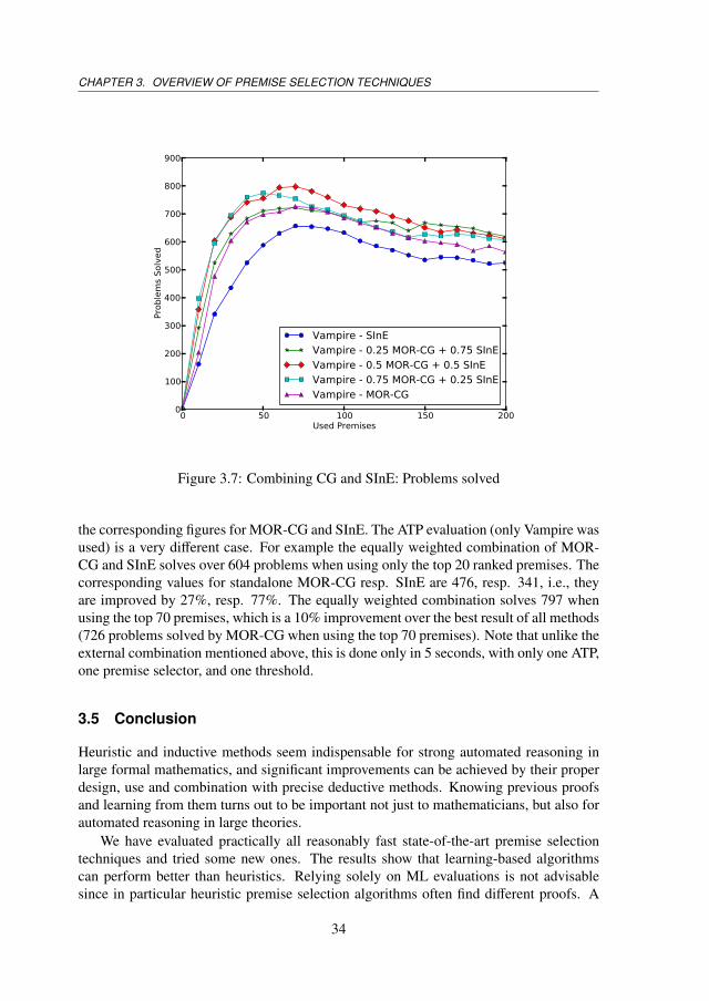
As a final experiment that opens the premise selection field to the application of ad-vanced ranking-aggregation methods, we have performed an initial simple evaluation ofcombining two very different premise ranking methods: MOR-CG and SInE. The aggre-gation is done by simple weighted linear combination, i.e., the final ranking is obtainedvia weighted linear combination of the predicted individual rankings. We test a limitedgrid of weights, in the interval of [0,1] with a step value of 0.25, i.e., apart from theoriginal MOR-CG and SInE rankings we get three more weighted aggregate rankings asfollows: 0.25 ∗CG + 0.75 ∗SInE, 0.5 ∗CG + 0.5 ∗SInE, and 0.75 ∗CG + 0.25 ∗SInE. Thefollowing Figure 3.7 shows their ATP evaluation.
The machine learning evaluation (done as before against the data extracted from thehuman proofs) is not surprising, and the omitted graphs look like linear combinations of
33
CHAPTER 3. OVERVIEW OF PREMISE SELECTION TECHNIQUES
0 50 100 150 200Used Premises
0
100
200
300
400
500
600
700
800
900Pr
oble
ms
Solv
ed
Vampire - SInEVampire - 0.25 MOR-CG + 0.75 SInEVampire - 0.5 MOR-CG + 0.5 SInEVampire - 0.75 MOR-CG + 0.25 SInEVampire - MOR-CG
Figure 3.7: Combining CG and SInE: Problems solved
the corresponding figures for MOR-CG and SInE. The ATP evaluation (only Vampire wasused) is a very different case. For example the equally weighted combination of MOR-CG and SInE solves over 604 problems when using only the top 20 ranked premises. Thecorresponding values for standalone MOR-CG resp. SInE are 476, resp. 341, i.e., theyare improved by 27%, resp. 77%. The equally weighted combination solves 797 whenusing the top 70 premises, which is a 10% improvement over the best result of all methods(726 problems solved by MOR-CG when using the top 70 premises). Note that unlike theexternal combination mentioned above, this is done only in 5 seconds, with only one ATP,one premise selector, and one threshold.
3.5 Conclusion
Heuristic and inductive methods seem indispensable for strong automated reasoning inlarge formal mathematics, and significant improvements can be achieved by their properdesign, use and combination with precise deductive methods. Knowing previous proofsand learning from them turns out to be important not just to mathematicians, but also forautomated reasoning in large theories.
We have evaluated practically all reasonably fast state-of-the-art premise selectiontechniques and tried some new ones. The results show that learning-based algorithmscan perform better than heuristics. Relying solely on ML evaluations is not advisablesince in particular heuristic premise selection algorithms often find different proofs. A
34

3.5. CONCLUSION
combination of heuristic and learning-based predictions gives the best results.
35

Chapter 4
Learning from Multiple Proofs
Mathematical textbooks typically present only one proof for most of the theorems. How-ever, there are infinitely many proofs for each theorem in first-order logic, and mathe-maticians are often aware of (and even invent new) important alternative proofs and usesuch knowledge for (lateral) thinking about new problems.In this chapter we explore how the explicit knowledge of multiple (human and ATP) proofsof the same theorem can be used in learning-based premise selection algorithms in large-theory mathematics. Several methods and their combinations are defined, and their effecton the ATP performance is evaluated on the MPTP2078 benchmark. The experimentsshow that the proofs used for learning significantly influence the number of problemssolved, and that the quality of the proofs is more important than the quantity.
4.1 Learning from Different Proofs
In the previous chapter we tested and evaluated several premise selection algorithms ona subset of the Mizar Mathematical Library (MML), the MPTP2078 large-theory bench-mark,1 using the (human) proofs from the MML as training data for the learning algo-rithms. We found that learning from such human proofs helps a lot, but alternative proofscan quite often be successfully constructed by ATPs, making heuristic methods like SInEsurprisingly strong and orthogonal to learning methods. Thanks to these experiments wenow also have (possibly several) ATP proofs for most of the problems.
In this chapter, we investigate how the knowledge of different proofs can be integratedin the machine learning algorithms for premise selection, and how it influences the perfor-mance of the ATPs. Section 4.2 introduces the necessary machine learning terminologyand explains how different proofs can be used in the algorithms. In Section 4.3, we define
This chapter is based on: [55] “Learning from Multiple Proofs: First Experiments”, published in theProceedings of the 3rd Workshop on Practical Aspects of Automated Reasoning.
1Available at http://wiki.mizar.org/twiki/bin/view/Mizar/MpTP2078.
37
CHAPTER 4. LEARNING FROM MULTIPLE PROOFS
several possible ways to use the additional knowledge given by the different proofs. Thedifferent proof combinations are evaluated and discussed in Section 4.4, and Section 4.5concludes.
4.2 The Machine Learning Framework and the Data
We start with the setting introduced in the previous chapter. Γ denotes the set of all factsthat appear in a given (fixed) large mathematical corpus (MPTP2078 in this chapter). Thecorpus is assumed to use notation (symbols) and formula names consistently, since theyare used to define the features and labels for the machine learning algorithms as definedin Chapter 2. The visibility relation over Γ is defined by the chronological growth of ITPlibrary.
We say that a proof P is a proof over Γ if the conjecture and all premises used in P areelements of Γ. Given a set of proofs ∆ over Γ in which every fact has at most one proof,the (∆-based) proof matrix µ∆ : Γ×Γ→ {0,1} is defined as
µ∆(c, p)B
1 if p is used to prove c in ∆,0 otherwise.
In other words, µ∆ is the adjacency matrix of the graph of the direct proof dependenciesfrom ∆. The proof matrix derived from the MML proofs, together with the formulafeatures are used as training data.
In the previous chapter, we compared several different premise selection algorithmson the MPTP2078 dataset. Thanks to this comparison we have ATP proofs for 1328 ofthe 2078 problems, found by Vampire 0.6 [77]. For some problems we found severaldifferent proofs, meaning that the sets of premises used in the proofs differ. Figure 4.1shows the number of different ATP proofs we have for each problem. The maximumnumber of different proofs is 49. On average, we found 6.71 proofs per solvable problem.
This database of proofs allows us to start considering multiple proofs for a c ∈ Γ. Foreach conjecture c, let Θc be the set of all ATP proofs of c in our dataset, and let nc denotethe cardinality of Θc. We use a generalized proof matrix to represented multiple proofsof c. The general interpretation of µX(c, p) is the relevance (weight) of a premise p for aproof of c determined by X, where X can either be a set of proofs as above, or a particularalgorithm (typically in conjunction with the data to which it is applied). For a single proofσ, let µσ B µ{σ}, i.e.,
µσ(c, p)B
1 if σ ∈ Θc and p is used to prove c in σ,0 otherwise.
We end this section by introducing the concept of redundancy, which seems to beat the heart of the problem that we are exploring. Let c be a conjecture and σ1,σ2 beproofs for c (σ1,σ2 ∈ Θc) with used premises {p1, p2} and {p1, p2, p3} respectively. Inthis case, premise p3 can be called redundant since we know a proof of c that does not
38
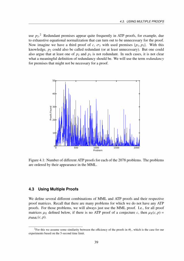
4.3. USING MULTIPLE PROOFS
use p3.2 Redundant premises appear quite frequently in ATP proofs, for example, dueto exhaustive equational normalization that can turn out to be unnecessary for the proof.Now imagine we have a third proof of c, σ3 with used premises {p1, p3}. With thisknowledge, p2 could also be called redundant (or at least unnecessary). But one couldalso argue that at least one of p2 and p3 is not redundant. In such cases, it is not clearwhat a meaningful definition of redundancy should be. We will use the term redundancyfor premises that might not be necessary for a proof.
0 500 1000 1500 2000Problem
0
10
20
30
40
50
Proo
fs F
ound
Figure 4.1: Number of different ATP proofs for each of the 2078 problems. The problemsare ordered by their appearance in the MML.
4.3 Using Multiple Proofs
We define several different combinations of MML and ATP proofs and their respectiveproof matrices. Recall that there are many problems for which we do not have any ATPproofs. For those problems, we will always just use the MML proof. I.e., for all proofmatrices µX defined below, if there is no ATP proof of a conjecture c, then µX(c, p) =
µMML(c, p).
2For this we assume some similarity between the efficiency of the proofs in Θc, which is the case for ourexperiments based on the 5-second time limit.
39
CHAPTER 4. LEARNING FROM MULTIPLE PROOFS
4.3.1 Substitutions and Unions
The simplest way to combine different proofs is to either only consider the used premisesof one proof, or take the union of all used premises. We consider five different combina-tions.
Definition 6 (MML Proofs).
µMML(c, p)B
1 if p is used to prove c in the MML proof,0 otherwise.
This dataset will be used as baseline throughout all experiments. It uses the humanproofs from the Mizar library.
Definition 7 (Random ATP Proof). For each conjecture c for which we have ATP proofs,pick a (pseudo)random ATP proof σc ∈ Θc.
µRandom(c, p)B
1 if p is a used premise in σc,0 otherwise.
Definition 8 (Best ATP Proof). For each conjecture c for which we have ATP proofs,pick an(y) ATP proof with the least number of used premises σmin
c ∈ Θc.
µBest(c, p)B
1 if p is a used premise in σminc ,
0 otherwise.
Definition 9 (Random Union). For each conjecture c for which we have ATP proofs, picka random ATP proof σc ∈ Θc.
µRandomUnion(c, p)B
1 if p is a premise used in σc or in the MML proof of c,0 otherwise.
Definition 10 (Union). For each conjecture c for which we have ATP proofs, we define
µUnion(c, p)B
1 if p is a premise used in any ATP or MML proof of c,0 otherwise.
4.3.2 Premise Averaging
Proofs can also be combined by learning from the average used premises. We considerthree options, the standard average, a biased average and a scaled average.
Definition 11 (Average). The average gives equal weight to each proof.
µAverage(c, p) =1
nc + 1
∑σ∈Θc
µσ(c, p) +µMML(c, p)
40
4.3. USING MULTIPLE PROOFS
The intuition is that the average gives a better idea of how necessary a premise reallyis. When there are very different proofs, the average will give a very low weight to everypremise. That is why we also tried scaling as follows:
Definition 12 (Scaled Average). The scaled average ensures that there is at least onepremise with weight 1.
µScaledAverage(c, p) =
∑σ∈Θc µσ(c, p) +µMML(c, p)
maxq∈Γ∑σ∈Θc µσ(c,q) +µMML(c,q)
Another experiment is to make the weight of all the ATP proofs equal to the weightof the MML proof:
Definition 13 (Biased Average).
µBiasedAverage(c, p) =12
(∑σ∈Θc µσ(c, p)
nc+µMML(c, p)
)4.3.3 Premise Expansion
Consider a situation where a ` b and b ` c. Obviously, not only b, but also a provesc. When we consider the used premises in a proof, we only use the information aboutthe direct premises (b in the example), but nothing about the indirect premises (a in theexample), the premises of the direct premises. Using this additional information mighthelp the learning algorithms. We call this premise expansion and define three differentweight functions that try to capture this indirect information. All three penalize the weightof the indirect premises with a factor of 1
2 .
Definition 14 (MML Expansion). For the MML expansion, we only consider the MMLproofs and their one-step expansions:
µMMLExp(c, p) = µMML(c, p) +
∑q∈Γ µMML(c,q)µMML(q, p)
2Note that since µMML(c, p) is either 0 or 1, the sum
∑q∈Γ µMML(c,q)µMML(q, p) just counts
how often p is a grandparent premise of c.
Definition 15 (Average Expansion). The average expansion takes µAverage instead ofµMML:
µAverageExp(c, p) = µAverage(c, p) +
∑q∈Γ µAverage(c,q)µAverage(q, p)
2Definition 16 (Scaled Expansion). And finally, we consider an expansion of the scaledaverage.
µScaledAverageExp(c, p) = µScaledAverage(c, p) +
∑q∈Γ µScaledAverage(c,q)µScaledAverage(q, p)
2Deeper expansions and different penalization factors are possible, but given the per-
formance of these initial tests shown in the next section we decided to not investigatefurther.
41
CHAPTER 4. LEARNING FROM MULTIPLE PROOFS
4.4 Results
4.4.1 Experimental Setup
All experiments were done on the MPTP2078 dataset. Because of its good performance inearlier evaluations, we used the Multi-Output-Ranking (MOR) learning algorithm for theexperiments. For each conjecture, MOR is allowed to train on all proofs that were (in thechronological order of MML) done up to that conjecture. In particular, this means that thealgorithms do not train on the data they were asked to predict. Three-fold cross validationon the training data was used to find the optimal parameters. For the combinations in4.3.1, the AUC measure was used to estimate the performance. The other combinationsused the square-loss error. For each of the 2078 problems, MOR predicts a ranking of thepremises.
We again use Vampire 0.6 for evaluating the predictions. Version 0.6 was chosento make the experiments comparable with the earlier results. Vampire is run with 5stime limit on an Intel Xeon E5520 2.27GHz server with 24GB RAM and 8MB CPUcache. Each problem is always assigned one CPU. For each MPTP2078 problem, wecreated 20 new problems, containing the 10,20, ...,200 highest ranked premises and ranVampire on each of them. The graphs show how many problems were solved using the10,20, ...,200 highest ranked premises. As a performance baseline, Vampire 0.6 in CASCmode (that means also using SInE with different parameters on large problems) can solve548 problems in 10 seconds [2].
4.4.2 Substitutions and Unions
Figure 4.2 shows the performance of the simple proof combinations introduced in 4.3.1. Itcan be seen that using ATP instead of MML proofs can improve the performance consid-erably, in particular when only few premises are provided. One can also see the differencethat the quality of the proof makes. The best ATP proof predictions always solved moreproblems than the random ATP proof predictions. Taking the union of two or more proofsdecreases the performance. This can be due to the redundancy introduced by consideringmany different premises and suggests that the ATP search profits most from a simple andclear (one-directional) advice, rather than from a combination of ideas.
4.4.3 Premise Averaging
Taking the average of the used premises could be a good way to combat the redundantpremises. The idea is that premises that are actually important should appear in almostevery proof, whereas premises that are redundant should only be present in a few proofs.Hereby, important premises should get a high weight and unimportant premises a lowweight. The results of the averaging combinations can be seen in Figure 4.3.2.
Apart from the scaled average, it seems that taking the average does perform betterthan taking the union. However, the baseline of only the MML premises is better oralmost as good as the average predictions.
42
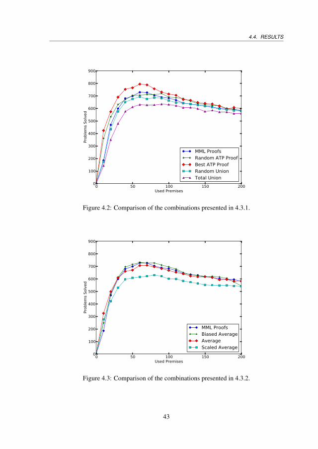
4.4. RESULTS
0 50 100 150 200Used Premises
0
100
200
300
400
500
600
700
800
900
Prob
lem
s So
lved
MML ProofsRandom ATP ProofBest ATP ProofRandom UnionTotal Union
Figure 4.2: Comparison of the combinations presented in 4.3.1.
0 50 100 150 200Used Premises
0
100
200
300
400
500
600
700
800
900
Prob
lem
s So
lved
MML ProofsBiased AverageAverageScaled Average
Figure 4.3: Comparison of the combinations presented in 4.3.2.
43
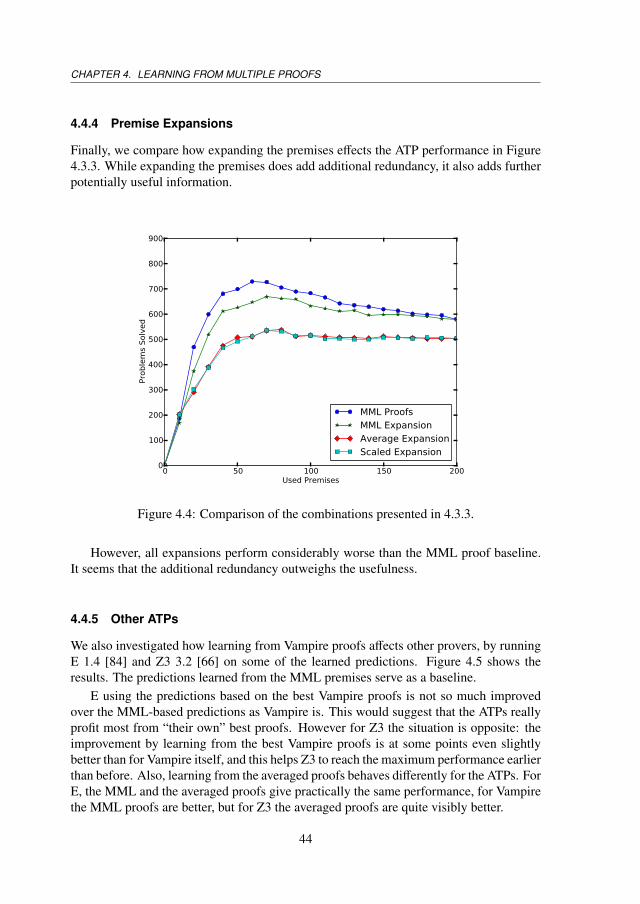
CHAPTER 4. LEARNING FROM MULTIPLE PROOFS
4.4.4 Premise Expansions
Finally, we compare how expanding the premises effects the ATP performance in Figure4.3.3. While expanding the premises does add additional redundancy, it also adds furtherpotentially useful information.
0 50 100 150 200Used Premises
0
100
200
300
400
500
600
700
800
900
Prob
lem
s So
lved
MML ProofsMML ExpansionAverage ExpansionScaled Expansion
Figure 4.4: Comparison of the combinations presented in 4.3.3.
However, all expansions perform considerably worse than the MML proof baseline.It seems that the additional redundancy outweighs the usefulness.
4.4.5 Other ATPs
We also investigated how learning from Vampire proofs affects other provers, by runningE 1.4 [84] and Z3 3.2 [66] on some of the learned predictions. Figure 4.5 shows theresults. The predictions learned from the MML premises serve as a baseline.
E using the predictions based on the best Vampire proofs is not so much improvedover the MML-based predictions as Vampire is. This would suggest that the ATPs reallyprofit most from “their own” best proofs. However for Z3 the situation is opposite: theimprovement by learning from the best Vampire proofs is at some points even slightlybetter than for Vampire itself, and this helps Z3 to reach the maximum performance earlierthan before. Also, learning from the averaged proofs behaves differently for the ATPs. ForE, the MML and the averaged proofs give practically the same performance, for Vampirethe MML proofs are better, but for Z3 the averaged proofs are quite visibly better.
44
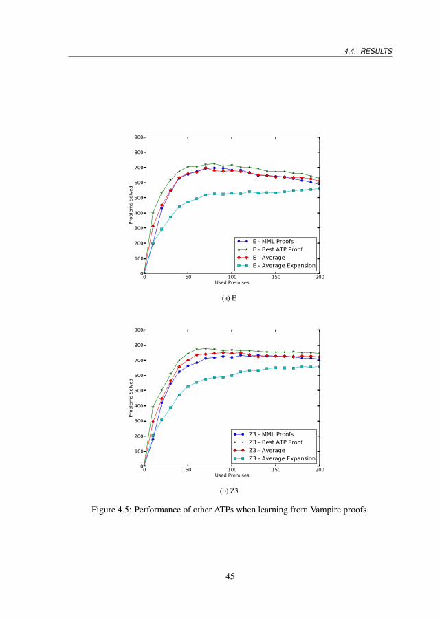
4.4. RESULTS
0 50 100 150 200Used Premises
0
100
200
300
400
500
600
700
800
900Pr
oble
ms
Solv
ed
E - MML ProofsE - Best ATP ProofE - AverageE - Average Expansion
(a) E
0 50 100 150 200Used Premises
0
100
200
300
400
500
600
700
800
900
Prob
lem
s So
lved
Z3 - MML ProofsZ3 - Best ATP ProofZ3 - AverageZ3 - Average Expansion
(b) Z3
Figure 4.5: Performance of other ATPs when learning from Vampire proofs.
45
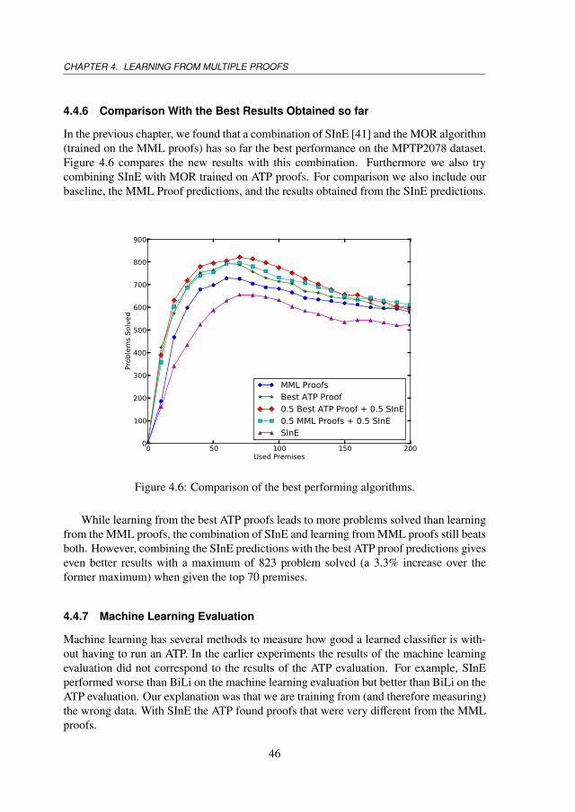
CHAPTER 4. LEARNING FROM MULTIPLE PROOFS
4.4.6 Comparison With the Best Results Obtained so far
In the previous chapter, we found that a combination of SInE [41] and the MOR algorithm(trained on the MML proofs) has so far the best performance on the MPTP2078 dataset.Figure 4.6 compares the new results with this combination. Furthermore we also trycombining SInE with MOR trained on ATP proofs. For comparison we also include ourbaseline, the MML Proof predictions, and the results obtained from the SInE predictions.
0 50 100 150 200Used Premises
0
100
200
300
400
500
600
700
800
900
Prob
lem
s So
lved
MML ProofsBest ATP Proof0.5 Best ATP Proof + 0.5 SInE0.5 MML Proofs + 0.5 SInESInE
Figure 4.6: Comparison of the best performing algorithms.
While learning from the best ATP proofs leads to more problems solved than learningfrom the MML proofs, the combination of SInE and learning from MML proofs still beatsboth. However, combining the SInE predictions with the best ATP proof predictions giveseven better results with a maximum of 823 problem solved (a 3.3% increase over theformer maximum) when given the top 70 premises.
4.4.7 Machine Learning Evaluation
Machine learning has several methods to measure how good a learned classifier is with-out having to run an ATP. In the earlier experiments the results of the machine learningevaluation did not correspond to the results of the ATP evaluation. For example, SInEperformed worse than BiLi on the machine learning evaluation but better than BiLi on theATP evaluation. Our explanation was that we are training from (and therefore measuring)the wrong data. With SInE the ATP found proofs that were very different from the MMLproofs.
46
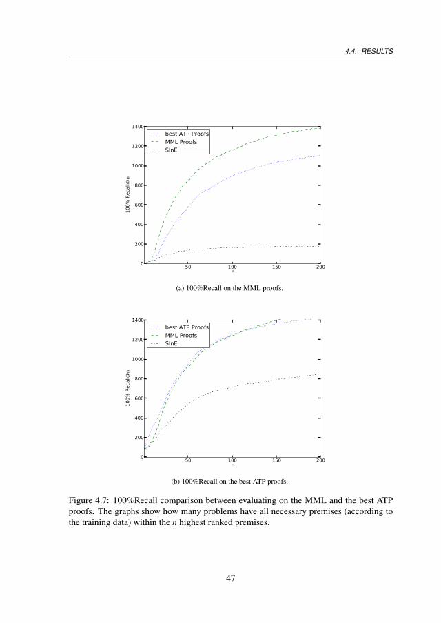
4.4. RESULTS
50 100 150 200n
0
200
400
600
800
1000
1200
140010
0% R
ecal
l@n
best ATP ProofsMML ProofsSInE
(a) 100%Recall on the MML proofs.
50 100 150 200n
0
200
400
600
800
1000
1200
1400
100%
Rec
all@
n
best ATP ProofsMML ProofsSInE
(b) 100%Recall on the best ATP proofs.
Figure 4.7: 100%Recall comparison between evaluating on the MML and the best ATPproofs. The graphs show how many problems have all necessary premises (according tothe training data) within the n highest ranked premises.
47
CHAPTER 4. LEARNING FROM MULTIPLE PROOFS
In Figure 4.7 we present a comparison between a machine learning evaluation (the100%Recall measure) depending on whether we evaluate on the MML proofs or on thebest ATP proofs. Ideally we would like to have that the machine learning performanceof the algorithms corresponds to the ATP performance (see Figure 4.6). This is clearlynot the case for the 100%Recall on the MML proofs graph. The best ATP predictions arebetter than the MML proof predictions, and SInE solves more than 200 problems. Withthe new evaluation, the 100%Recall on the best ATP proofs graph, the performance ismore similar to the actual ATP performance but there is still room for improvement.
4.5 Conclusion
The fact that there is never only one proof makes premise selection an interesting machinelearning problem. Since it is in general undecidable to know the “best prediction”, thedomain has a randomness aspect that is quite unusual (Chaitin-like [22]) in AI.
In this chapter we experimented with different proof combinations to obtain betterinformation for high-level proof guidance by premise selection. We found that it is easyto introduce so much redundancy that the predictions created by the learning algorithmsare not good for existing ATPs. On the other hand we saw that learning from proofs withfew premises (and hence probably less redundancy) increases the ATP performance. Itseems that we should look for a measure of how ‘good’ or ‘simple’ a proof is, and onlylearn from the best proofs. Such measures could be for example the number of inferencesteps done by the ATP during the proof search, or the total CPU time needed to find theproof.
Another question that was (at least initially) answered in this chapter is to what extentlearning from human proofs can help an ATP, in comparison to learning from ATP proofs.We saw that while not optimal, learning from human proofs seems to be approximatelyequivalent to learning from suboptimal (for example random, or averaged) ATP proofs.Learning from the best ATP proof is about as good as combining SInE with learningfrom the MML proofs. Combining SInE with learning from the best ATP proof stilloutperforms all methods.
48
Chapter 5
Automated and Human Proofs in GeneralMathematics
First-order translations of large mathematical repositories allow discovery of new proofsby automated reasoning systems. Large amounts of available mathematical knowledgecan be re-used by combined AI/ATP systems, possibly in unexpected ways. But automatedsystems can be also more easily misled by irrelevant knowledge in this setting, and findingdeeper proofs is typically more difficult. Both large-theory AI/ATP methods, and trans-lation and data-mining techniques of large formal corpora, have significantly developedrecently, providing enough data for an initial comparison of the proofs written by mathe-maticians and the proofs found automatically. This chapter describes such a comparisonconducted over the 52000 mathematical theorems from the Mizar Mathematical Library.
5.1 Introduction: Automated Theorem Proving in Mathematics
Computers are becoming an indispensable part of many areas of mathematics [38]. Astheir capabilities develop, human mathematicians are faced with the task of steering, com-prehending, and evaluating the ideas produced by computers, similar to the players ofchess in recent decades. A notable milestone is the automatically found proof of theRobbins conjecture by EQP [62] and its postprocessing into a human-comprehensibleproof by ILF [25] and Mathematica [29]. Especially in small equational algebraic theories(e.g., quasigroup theory), a number of nontrivial proofs have been already found auto-matically [74], and their evaluation, understanding, and automated post-processing is anopen problem [113].
This chapter is based on: [3] “Automated and Human Proofs in General Mathematics: An Initial Compar-ison”, published in the Proceedings of the 18th International Conference on Logic for Programming, ArtificialIntelligence, and Reasoning. All three authors contributed equally to the paper. Part of Section 5.2.1 is takenfrom [2] “Premise Selection for Mathematics by Corpus Analysis and Kernel Methods”, published in the Journalof Automated Reasoning.
49
CHAPTER 5. AUTOMATED AND HUMAN PROOFS IN GENERAL MATHEMATICS
In the recent years, large general mathematical corpora like the Mizar Mathemati-cal Library (MML) and the Isabelle/HOL library are being made available to automatedreasoning and AI methods [102, 73], leading to the development of automated reasoningtechniques working in large theories with many previous theorems, definitions, and proofsthat can be re-used [110, 41, 64, 112]. A recent evaluation (and tuning) of ATP systemson the MML [108] has shown that the Vampire/SInE [77] system can already re-prove39% of the MML’s 52000 theorems when the necessary premises are precisely selectedfrom the human1 proofs, and about 14% of the theorems when the ATP is allowed to usethe whole available library, leading on average to 40000 premises in such ATP problems.In the previous chapters we showed that re-using (generalizing and learning) the knowl-edge accumulated in previous proofs can further significantly improve the performanceof combined AI/ATP systems in large-theory mathematics.
This performance, and the recently developed proof analysis for the MML [4], al-lowed an experiment with finding automatically all proofs in the MML by a combinationof learning and ATP methods. This is described in Section 5.2. The 9141 ATP proofsfound automatically were then compared using several metrics to the human proofs inSection 5.3 and Section 5.4.
5.2 Finding proofs in the MML with AI/ATP support
To create a sufficient body of ATP proofs from the MML, we have conducted a largeAI/ATP experiment that makes use of several recently developed techniques and signifi-cant computational resources. The basic idea of the experiment is to lift the setting usedin [2] for large-theory automated proving of the MPTP2078 benchmark to the wholeMML (approximately 52000 theorems and more than 100000 premises). The settingconsists of the following three consecutive steps:
• mining proof dependencies from all MML proofs;
• learning premise selection from the mined proof dependencies;
• using an ATP to prove new conjectures from the best selected premises.
5.2.1 Mining the dependencies from all MML proofs
For the experiments below, we used Alama et al.’s method for computing fine-grained de-pendencies [4]. The first step in the computation is to break up each article in the MMLinto a sequence of Mizar texts, each consisting of a single statement (e.g., a theorem, def-inition, unexported lemma). Each of these texts can—with suitable preprocessing—beregarded as a complete, valid Mizar article in its own right. The decomposition of a whole
1Mizar proofs are initially human-written, but they are formal and machine-understandable. That allowstheir automated machine processing and refactoring, which can make them “less human”. Yet, we believe thattheir classification as “human” is appropriate, and that MML/MPTP is probably the most suitable resource todayfor attempting this initial comparison of ATP and human proofs.
50
5.2. FINDING PROOFS IN THE MML WITH AI/ATP SUPPORT
MML article into such smaller articles typically requires a number of nontrivial refac-toring steps, comparable, e.g., to automated splitting and re-factoring of large programswritten in programming languages with complicated syntactic mechanisms.
In Mizar, every article has a so-called environment: a list ENV0 = [statement j : 1 ≤ j ≤length(ENV0)] of statements statement j specifying the background knowledge (theorems,notations, etc.) that is used to verify the article. The actual Mizar content contained in anarticle’s environment, is, in general, a rather conservative overestimate of the statementsthat the article actually needs. The algorithm first defines the current environment asENV0. It then considers each statement in ENV0 and tries to verify the article usingthe current environment without the considered statement. If the verification succeeds,the considered statement is deleted from the current environment. To be more precises,starting with the original environment ENV0 (in which the article verification succeeds),the algorithm works by constructing a sequence of finer environments {ENVi : 1 ≤ i ≤length(ENV0)} such that
ENVi B
ENVi−1 if the verification fails in ENVi−1−{statementi}ENVi−1−{statementi} otherwise .
The article verification thus still succeeds in the final ENVlength(ENV0) environment, andthis environment consist of all the statement of ENV0 whose removal caused the articleverification to fail during this construction.2 The dependencies of the original statement,which formed the basis of the article, are then defined as the elements of ENVlength.
This process is in detail described in [4], where it is conducted for the 100 initialarticles from the MML. The computation takes several days for all of MML, howeverthe information thus obtained gives rise to an unparalleled corpus of data about human-written proofs in the largest available formal body of mathematics. In the final account,the days of computation pay off, by providing more precise advice for proving new con-jectures over the whole MML. An approximate estimate of the computational resourcestaken by this job is about ten days of full (parallel) CPU load (12 hyperthreading Xeon2.67 GHz cores, 24 GB RAM) of the Mizar server at the University of Alberta. Theresulting dependencies for all MML items can be viewed online.3
5.2.2 Learning Premise Selection from Proof Dependencies
To learn premise selection from proof dependencies, one characterizes all MML formulasby suitable features, and feeds them (together with the detailed proof information) to amachine learning system that is trained to advise premises for later conjectures. Formulasymbols have been used previously for this task in [102]. Thanks to sufficient hardwarebeing available, we have for the first time included also term features generated by theMaLARea framework, added to it in 2008 [110] for experiments with smaller subsets of
2Note that this final environment could in general still be made smaller (after the removal of a certainstatement, another statement might become unnecessary), and its construction depends on the (chosen and fixedfor all experiments) initial ordering of statements in the environment.
3http://mizar.cs.ualberta.ca/mizar-items
51
CHAPTER 5. AUTOMATED AND HUMAN PROOFS IN GENERAL MATHEMATICS
MML. Thus, for each MML formula we include as its characterization also all the sub-terms and subformulas contained in the formula, which makes the learning and predictionmore precise. To our surprise, the EPROVER-based [84] utility that consistently numbersall shared terms in all formulas, written for this purpose in 2008 by Josef Urban, scaledwithout problems to the whole MML. This feature-generation phase took only minutesand created over one million features. We have also briefly explored using validity infinite models (introduced in MaLARea in 2008, building on Pudlák’s previous work [76])as a more semantic way of characterizing formulas. However, this has turned out tobe very time-consuming, most likely caused by the LADR-based clausefilter utilitystruggling with evaluating in the models some complicated (containing many quantifiers)mathematical formulas. Clearly, further optimizations are needed for extracting such se-mantic characterizations for all of MML. Even without such features, the machine learn-ing was already pushed to the limit. The kernel-based multi-output ranker presented inchapter 2.2.4 turned out to be too slow and memory-exhaustive to handle over one millionfeatures and over hundred thousand training examples. The SNoW system used in naiveBayes mode took several gigabytes of RAM to train on the data, and on average about asecond (ca. a day of computation for all of MML) to produce a premise prediction foreach MML problem (based always on incremental training4 on all previous MML proofs).The results of this run are SNoW premise predictions for all of MML, available online5
as the raw SNoW output, and also postprocessed into corresponding ATP problems (seebelow).
5.2.3 Using ATPs to Prove the Conjectures from the Selected Premises
As the MML grows from axioms of set theory to advanced mathematics, it gives rise toa chronological ordering of its theorems. When a new theorem C is conjectured, all theprevious theorems and definitions are available as premises, and all the previous proofsare used to learn which of these premises are relevant for C. The SNoW system providesa ranking of all premises, and the best premises are given to an ATP which attempts aproof of C.
There are many ways how to organize several ATP systems to try to prove C, withdifferent numbers of the highest ranked premises and with different time limits. For ourexperiments, we have fixed the ATP system to be Vampire (version 1.8) [77], and we havealways used the 200 highest ranked premises and a time limit of 20 seconds. A 12-core2.67 GHz Xeon server at University of Alberta was used for (parallelized) proving, whichtook about a day in real time. This has produced 9141 automatically found proofs thatwe further analyze. The overall success rate is over 18% of theorems proved which is sofar the best result on the whole MML, but we have not really focused yet on getting thisas high as possible. For example, running Vampire in parallel with both 40 and 200 bestrecommended premises has been shown to significantly improve the success rate, anda preliminary experiment with the Z3 solver has provided another two thousand proofs
4In the incremental learning mode, the evaluation and training are done at the same time for each example,hence there was no extra time taken by training.
5http://mizar.cs.ualberta.ca/~mptp/proofcomp/snow_predictions.tar.gz
52
5.3. PROOF METRICS
from the problems with 200 best premises. Unfortunately, Z3 does not (yet) print thenames of premises used in the proofs, so its proofs would not be directly usable for theanalysis that is conducted here. When using a large number of premises, an ATP proof canoften contain unnecessary premises. To weed out those unnecessary premises, we alwaysre-run the ATP with only the premises that were used in the first run. The ATP problemsare also available online6 for further experiments, as well as all the proofs found.7
5.3 Proof Metrics
We thus have, for 9141 Mizar theorems φ, the set of premises that were used in the (min-imized) ATP proof of φ. Each ATP proof was found completely independently of itsMizar proof, i.e., no information (e.g., about the premises used) from the Mizar proof wastransferred to the ATP proof.8 This gives us a notion of dependency for Mizar theorems,derived from an ATP. From the Mizar proof dependency analysis we also know preciselywhat Mizar items are needed for a given Mizar (human-written) proof to be successful.
Definition 17. For a Mizar theorem φ, let PMML(φ) be the minimal set of premises neededfor the success of the (human) MML proof of φ. Let PATP(φ) be the set of premises usedby an ATP to prove φ.
This gives rise to the notions of “immediate dependence” and “indirect dependence”of one Mizar item a upon another Mizar item b:
Definition 18. For Mizar items a and b, a <1 b means that a immediately depends onb (b ∈ PMML(a)). Let < be the transitive closure of <1, ≤ its reflexive version, and letP∗MML(a)B {b : b < a}. For a set S of items, let P∗MML(S )B {b : ∃a ∈ S : b ≤ a} .
While theoretically, there are multiple versions of <1 and < induced by different (ATP,Mizar) proofs, unless we explicitly state otherwise, these relations will always refer to thedependencies derived from the Mizar proofs. The pragmatic reason is that we do not havean ATP proof for all Mizar items,9 and hence we do not have the full dependency graphinduced by ATP proofs. Also, the way ATP proofs were produced was by always relyingon the previous Mizar theorems and dependency data, therefore it makes sense to also usethe Mizar data for the transitive closure.
We define two comparison metrics. D (Dependencies) counts the number of premisesused in a proof.
Definition 19. For each Mizar item a, we define its Mizar dependencies as DMML(a)B|PMML(a)| and its ATP dependencies via DATP(a)B |PATP(a)|.
6http://mizar.cs.ualberta.ca/~mptp/proofcomp/advised200f1.tar.gz7http://mizar.cs.ualberta.ca/~mptp/proofcomp/proved200f1min.tar.gz8The ATP proofs are however always based on the same state of previous theory and proof knowledge.
This could be further relaxed in future experiments.9We have limited the ATP experiment to Mizar theorems, so even with perfect ATP success rate we would
still miss for example all ATP dependencies of Mizar definitions, that often require proofs of existence, unique-ness, etc.
53
CHAPTER 5. AUTOMATED AND HUMAN PROOFS IN GENERAL MATHEMATICS
The second metric L (Length) adds weighting by (recursive) proof complexity. Forthe Mizar proofs, L is computed using the assumption that the Mizar weak refutationalchecker enforces a relatively uniform degree of derivational complexity on all Mizar proofsteps, which roughly correspond to proof lines in Mizar formalizations. For the ATPversion, we make a similar assumption that the complexity of ATP proof steps is roughlyuniform.10 For the comparison with human proofs, we define a conversion ratio c betweenthe number of ATP inference lines and the corresponding number of Mizar proof lines.This is pragmatically estimated as the average of such ratios for all the proofs where theATP used the same premises as the Mizar proof. The actual value computed (based on1223 proofs where PATP(a) = PMML(a)) is c = 81.99 . Formally:
Definition 20. For a Mizar-proved item a, let LMML(a) be the number of Mizar lines ofcode used to prove a (direct Mizar proof length). For each ATP-proved item a, let L0
ATP(a)be the number of steps in the ATP proof. Let EMML=AT P B {a : PATP(a) = PMML(a)}(items whose ATP and Mizar proofs use the same premises). The length conversion ratioc is defined as
cB1
|EMML=AT P|
∑a∈EMML=AT P
L0ATP(a)
LMML(a)
Finally, we define the normalized ATP proof length as LATP(a)B L0ATP(a)/c . For a set of
items S , let again LMML(S )B∑
a∈S LMML(a).
Definition 21. For a Mizar theorem a we set L∗MML(a)B LMML(a) + LMML(P∗MML(a)). Ifwe have an ATP proof, we define L∗ATP(a)B LATP(a) + LMML(P∗MML(PATP(a))).
The reason for using LMML and P∗MML in the recursive part of L∗ATP is again the factthat we only have the complete line count information for the Mizar proofs. Note that inL∗ we always count any lemma on the transitive proof path exactly once. We believe thatthis approach captures the mathematician’s intuition of proof complexity as the set of “theproofs that need to be understood” rather than as their multiset.
5.4 Evaluation
The metrics developed above were used to compare the Mizar and ATP proofs. The de-tailed evaluation data corresponding to this section are available online.11 First we ana-lyze the data based on the relation between PMML and PATP. For each Mizar theorem φthat can be proved by an ATP, we have either PMML(φ) = PATP(φ), PMML(φ) ⊂ PATP(φ),PATP(φ) ⊂ PMML(φ), or neither set is included in the other. Let us say that two sets A andB are orthogonal if neither A ⊆ B, nor B ⊆ A. The statistics is given in Table 5.1.
More than 10% (1223) of the proofs have the same dependencies. For 386 proofs,the MML proof depends on fewer premises than the ATP proof. While the orthogonal
10The precision of such metrics could be further improved, for example by expanding Vampire proofs intothe (really uniform) detailed proof objects developed for Otter/Prover9/IVY [63].
11http://mizar.cs.ualberta.ca/~mptp/proofcomp/metrics_evaluation.xls
54
5.4. EVALUATION
Table 5.1: Dependency statistics
PATP = PMML PATP ⊂ PMML PMML ⊂ PATP Orthogonal
Cases 1223 1980 386 5552
Min DATP 0 0 1 1Min DMML 0 1 1 1
Max DATP 7 12 89 63Max DMML 7 59 10 58Max |DMML−DATP| 0 58 83 60
Avg DATP 2.18 2.20 6.24 5.22Avg DMML 2.18 5.58 2.41 6.33Avg |DMML−DATP| 0 3.40 3.88 3.86
category is largest with 5552 proofs as was expected, it is surprising to see that 1980 ATPproofs (21.66%) depend on fewer premises. We found several possible explanations:• The ATP is naturally oriented towards finding short proofs. Getting involved proofs
with many premises is hard, and it may well be the main reason of ATP failureoutside the 9141 proved theorems.• In many cases, a human formalizer can overlook the fact that the same or very sim-
ilar theorem is already in the library.12 An example is the theorem LOPBAN_3:2413
which required a 20-line proof in Mizar, but the ATP found an earlier more generaltheorem BHSP_4:3 that (using additional typing information) provides an almostimmediate proof.• ATPs work in untyped first-order logic, and they are not constrained by the Mizar’s
(and other ITPs’) requirement that all types should be inhabited. For example, Mizarproof checking of GOEDELCP:114 fails if two type non-emptiness declarations areremoved, because the formula is no longer well-typed. The ATP proof howeverdoes not need any of them.
An interesting case is when the ATP finds a way to re-use previous lemmas. Sometimesenough knowledge about advanced concepts is already developed that can be used fortheir quite simple (“algebraic”) manipulation, abstracting from their definitions. An ex-ample is COMSEQ_3:4015, proving the relation between the limit of a complex sequenceand its real and imaginary parts. The human proof expands the definitions (finding a suit-able n for a given ε). The ATP just notices that this kind of groundwork was already donein a “similar” case COMSEQ_3:3916, and notices the “similarity” (algebraic simplification)
12From this point of view, this analysis is conducted at the right time, because the ATP service is starting tobe used by authors, and such simple repetitions will be prevented by it.
13http://mizar.cs.ualberta.ca/~mptp/cgi-bin/browserefs.cgi?refs=t24_lopban_3, The theoremsays that the partial-sums operator on normed space sequences commutes with multiplication by a scalar.
14http://mizar.cs.ualberta.ca/~mptp/cgi-bin/browserefs.cgi?refs=t1_goedelcp15http://mizar.cs.ualberta.ca/~mptp/cgi-bin/browserefs.cgi?refs=t40_comseq_316http://mizar.cs.ualberta.ca/~mptp/cgi-bin/browserefs.cgi?refs=t39_comseq_3
55
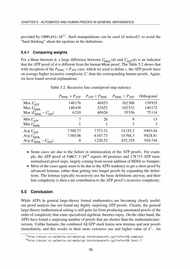
CHAPTER 5. AUTOMATED AND HUMAN PROOFS IN GENERAL MATHEMATICS
provided by COMPLEX1:2817. Such manipulations can be used (if noticed!) to avoid the“hard thinking” about the epsilons in the definitions.
5.4.1 Comparing weights
For a Mizar theorem φ, a large difference between L∗MML(φ) and L∗ATP(φ) is an indicatorthat the ATP proof of φ is different from the human Mizar proof. The Table 5.2 shows thatwith exception of the PMML = PATP case, which we used to define c, the ATP proofs haveon average higher recursive complexity L∗ than the corresponding human proofs. Again,we have found several explanations:
Table 5.2: Recursive line count/proof step statistics
PMML = PATP PATP ⊂ PMML PMML ⊂ PATP Orthogonal
Max L∗ATP 140176 40653 162308 139935Max L∗MML 140438 32652 162532 140172Max |L∗MML−L∗ATP| 6210 40626 35536 75114
Min L∗ATP 7 26 9 13Min L∗MML 1 1 3 3
Avg L∗ATP 7390.77 7373.31 14155.3 9893.04Avg L∗MML 7385.06 6167.73 14768.3 9828.81Avg |L∗MML−L∗ATP| 0 1220.52 632.329 910.744
• Some cases are due to the failure in minimization of the ATP proofs. For exam-ple, the ATP proof of FUNCT_7:2018 reports 40 premises and 178715 ATP (non-normalized) proof steps, largely coming from recent addition of BDDs to Vampire.• Most of the cases again seem to be due to the ATPs tendency to get a short proof by
advanced lemmas, rather than getting into longer proofs by expanding the defini-tions. The lemmas typically recursively use the basic definitions anyway, and theirline complexity is then a net contribution to the ATP proof’s recursive complexity.
5.5 Conclusion
While ATPs in general large-theory formal mathematics are becoming clearly useful,our proof analysis has not found any highly surprising ATP proofs. Clearly, the generallarge-theory mathematical setting is still quite far from producing automated proofs of theorder of complexity that some specialized algebraic theories enjoy. On the other hand, theATPs have found a surprising number of proofs that are shorter than the mathematicians’version. Unlike humans, the combined AI/ATP stack learns new lemmas and new proofsimmediately, and this results in their more extensive use and higher value of L∗. An
17http://mizar.cs.ualberta.ca/~mptp/cgi-bin/browserefs.cgi?refs=t28_complex118http://mizar.cs.ualberta.ca/~mptp/cgi-bin/browserefs.cgi?refs=t20_funct_7
56
5.5. CONCLUSION
ATP working in unsorted FOL can sometimes find proofs that, in some sense, get tothe “mathematical heart” of a theorem without first going through the syntactic hoopsof ensuring that terms have suitable sorts. The tools produced for our experiments canproduce information that is useful for maintainers of large formal libraries. We foundcases where an ATP was able to find a significantly shorter proof—sometimes employingonly one premise—compared to a human proof. At times, such highly efficient ATPproofs were due to duplication in the library or failure to use a generalization to prove aspecial case. Finally, this work could provide a practical “test bed” for theoretical criteriaof proof identity [27].
57

Chapter 6
MaSh - Machine Learning forSledgehammer
Sledgehammer integrates automated theorem provers into the proof assistant Isabelle. Akey component, the relevance filter, heuristically ranks the thousands of facts availableand selects a subset, based on syntactic similarity to the current goal. We introduce MaSh,an alternative that learns from successful proofs. New challenges arose from our “zero-click” vision: MaSh should integrate seamlessly with the users’ workflow, so that theybenefit from machine learning without having to install software, set up servers, or guidethe learning. The underlying machinery draws on recent research in the context of Mizarand HOL Light, with a number of enhancements. MaSh outperforms the old relevancefilter on large formalizations, and a particularly strong filter is obtained by combiningthe two filters.
6.1 Introduction
Sledgehammer [73] is a subsystem of the proof assistant Isabelle/HOL [68] that dis-charges interactive goals by harnessing external automated theorem provers (ATPs). Itheuristically selects a number of relevant facts1 (axioms, definitions, or lemmas) fromthe thousands available in background libraries and the user’s formalization, translatesthe problem to the external provers’ logics, and reconstructs any machine-found proof inIsabelle (Section 6.2). The tool is popular with both novices and experts.
Various aspects of Sledgehammer have been improved since its introduction, notablythe addition of SMT solvers [16], the use of sound translation schemes [14], close coop-
This chapter is based on: [56] “MaSh: Machine Learning for Sledgehammer”, published in the Proceed-ings of the 4th International Conference on Interactive Theorem Proving.
1To keep with the standard Isabelle terminology the notation differs from the previous chapters. We uselemma instead of statement, fact instead of premise, and goal instead of conjecture.
59
CHAPTER 6. MASH - MACHINE LEARNING FOR SLEDGEHAMMER
eration with the first-order superposition prover SPASS [17], and of course advances inthe underlying provers themselves. Together, these enhancements increased the successrate from 48% to 64% on the representative “Judgment Day” benchmark suite [20, 17].
One key component that has received little attention is the relevance filter. Meng andPaulson [64] designed a filter, MePo, that iteratively ranks and selects facts similar tothe current goal, based on the symbols they contain. Despite its simplicity, and despiteadvances in prover technology [41, 17, 86], this filter greatly increases the success rate:Most provers cannot cope with tens of thousands of formulas, and translating so manyformulas would also put a heavy burden on Sledgehammer. Moreover, the translation ofIsabelle’s higher-order constructs and types is optimized globally for a problem—smallerproblems make more optimizations possible, which helps the automated provers.
Coinciding with the development of Sledgehammer and MePo, a line of researchhas focused on applying machine learning to large-theory reasoning. Much of this workhas been done on the vast Mizar Mathematical Library (MML) [1], either in its originalMizar [61] formulation or in first-order form as the Mizar Problems for Theorem Prov-ing (MPTP) [104]. The MaLARea system [105, 110] and the competitions CASC LTBand Mizar@Turing [95] have been important milestones. Recently, comparative studiesinvolving MPTP [57, 2] and the Flyspeck project in HOL Light [45] have found that factselectors based on machine learning outperform purely symbol-based approaches.
Several learning-based advisors have been implemented and have made an impacton the automated reasoning community. In this chapter, we describe a tool that aimsto bring the fruits of this research to the Isabelle community. This tool, MaSh, offersan alternative to MePo by learning from successful proofs, whether human-written ormachine-generated.
Sledgehammer is a one-click technology—fact selection, translation, and reconstruc-tion are fully automatic. For MaSh, we had four main design goals:
• Zero-configuration: The tool should require no installation or configuration steps,even for use with unofficial repository versions of Isabelle.
• Zero-click: Existing users of Sledgehammer should benefit from machine learning,both for standard theories and for their custom developments, without having tochange their workflow.
• Zero-maintenance: The tool should not add to the maintenance burden of Isabelle.In particular, it should not require maintaining a server or a database.
• Zero-overhead: Machine learning should incur no overhead to those Isabelle userswho do not employ Sledgehammer.
By pursuing these “four zeros,” we hope to reach as many users as possible and keep themfor as long as possible. These goals have produced many new challenges.
MaSh’s heart is a Python program that implements a custom version of a weightedsparse naive Bayes algorithm that is faster than the naive Bayes algorithm implementedin the SNoW [21] system used in previous studies (Section 6.3). The program maintains
60
6.2. SLEDGEHAMMER AND MEPO
a persistent state and supports incremental, nonmonotonic updates. Although distributedwith Isabelle, it is fully independent and could be used by other proof assistants, auto-mated theorem provers, or applications with similar requirements.
This Python program is used within a Standard ML module that integrates machinelearning with Isabelle (Section 6.4). When Sledgehammer is invoked, it exports new factsand their proofs to the machine learner and queries it to obtain relevant facts. The maintechnical difficulty is to perform the learning in a fast and robust way without interferingwith other activities of the proof assistant. Power users can enhance the learning by lettingexternal provers run for hours on libraries, searching for simpler proofs.
A particularly strong filter, MeSh, is obtained by combining MePo and MaSh. Thethree filters are compared on large formalizations covering the traditional application ar-eas of Isabelle: cryptography, programming languages, and mathematics (Section 6.5).These empirical results are complemented by Judgment Day, a benchmark suite that hastracked Sledgehammer’s development since 2010. Performance varies greatly dependingon the application area and on how much has been learned, but even with little learningMeSh emerges as a strong leader.
6.2 Sledgehammer and MePo
Whenever Sledgehammer is invoked on a goal, the MePo (Meng–Paulson) filter selectsn facts φ1, . . . ,φn from the thousands available, ordering them by decreasing estimatedrelevance. The filter keeps track of a set of relevant symbols—i.e., (higher-order) con-stants and fixed variables—initially consisting of all the goal’s symbols. It performs thefollowing steps iteratively, until n facts have been selected:
1. Compute each fact’s score, as roughly given by r/(r + i), where r is the number ofrelevant symbols and i the number of irrelevant symbols occurring in the fact.
2. Select all facts with perfect scores as well as some of the remaining top-scoringfacts, and add all their symbols to the set of relevant symbols.
The implementation refines this approach in several ways. Chained facts (insertedinto the goal by means of the keywords using, from, then, hence, and thus) take absolutepriority; local facts are preferred to global ones; first-order facts are preferred to higher-order ones; rare symbols are weighted more heavily than common ones; and so on.
MePo tends to perform best on goals that contain some rare symbols; if all the symbolsare common, it discriminates poorly among the hundreds of facts that could be relevant.There is also the issue of starvation: The filter, with its iterative expansion of the setof relevant symbols, effectively performs a best-first search in a tree and may thereforeignore some relevant facts close to the tree’s root.
The automated provers are given prefixes φ1, . . . ,φm of the selected n facts. The orderof the facts—the estimated relevance—is exploited by some provers to guide the search.Although Sledgehammer’s default time limit is 30 s, the automated provers are invokedrepeatedly for shorter time periods, with different options and different number of facts
61
CHAPTER 6. MASH - MACHINE LEARNING FOR SLEDGEHAMMER
m ≤ n; for example, SPASS is given as few as 50 facts in some slices and as many as 1000in others. Excluding some facts restricts the search space, helping the prover find deeperproofs within the allotted time, but it also makes fewer proofs possible.
The supported ATP systems include the first-order provers E [85], SPASS [17], andVampire [77]; the SMT solvers CVC3 [8], Yices [28], and Z3 [66]; and the higher-orderprovers LEO-II [9] and Satallax [19].
Once a proof is found, Sledgehammer minimizes it by invoking the prover repeatedlywith subsets of the facts it refers to. The proof is then reconstructed in Isabelle by asuitable proof text, typically a call to the built-in resolution prover Metis [43].
Example 2. Given the goal
map f xs = ys =⇒ zip (rev xs) (rev ys) = rev (zip xs ys)
MePo selects 1000 facts: rev_map, rev_rev_ident, . . . , add_numeral_special(3). Theprover E, among others, quickly finds a minimal proof involving the 4th and 16th facts:
zip_rev: length xs = length ys =⇒ zip (rev xs) (rev ys) = rev (zip xs ys)length_map: length (map f xs) = length xs
Example 3. MePo’s tendency to starve out useful facts is illustrated by the followinggoal, taken from Paulson’s verification of cryptographic protocols [72]:
used [] ⊆ used evs
A straightforward proof relies on these four lemmas:
used_Nil: used [] =⋃
B parts (initState B)initState_into_used: X ∈ parts (initState B) =⇒ X ∈ used evs
subsetI: (∧
x. x ∈ A =⇒ x ∈ B) =⇒ A ⊆ BUN_iff : b ∈
⋃x∈A B x ←→ ∃x∈A. b ∈ B x
The first two lemmas are ranked 6807th and 6808th, due to the many initially irrelevantconstants (
⋃, parts, initState, and ∈). In contrast, all four lemmas appear among MaSh’s
first 45 facts and MeSh’s first 77 facts.
6.3 The Machine Learning Engine
MaSh (Machine Learning for Sledgehammer) is a Python program for fact selection withmachine learning.2 Its default learning algorithm is an approximation of naive Bayesadapted to fact selection. MaSh can perform fast model updates, overwrite data points,and predict the relevance of each fact. The program can also use the slower naive Bayesalgorithm implemented by SNoW [21].
2The source code is distributed with Isabelle2013 in the directory src/HOL/Tools/Sledgehammer/MaSh/src.
62
6.3. THE MACHINE LEARNING ENGINE
6.3.1 Basic Concepts
MaSh manipulates theorem proving concepts such as facts and proofs in an agnostic way,as “abstract nonsense”:
• A fact φ is a string.
• A feature f is also a string. A positive weight w is attached to each feature.
• Visibility is a partial order ≺ on facts. A fact φ is visible from a fact φ′ if φ ≺ φ′, andvisible through the set of facts Φ if there exists a fact φ′ ∈ Φ such that φ � φ′.
• The parents of a fact are its (immediate) predecessors with respect to ≺.
• A proof Π for φ is a set of facts visible from φ.
Facts are described abstractly by their feature sets. The features may for example bethe symbols occurring in a fact’s statement. Machine learning proceeds from the hypoth-esis that facts with similar features are likely to have similar proofs.
6.3.2 Input and Output
MaSh starts by loading the persistent model (if any), executes a list of commands, andsaves the resulting model on disk. The commands and their arguments are
learn fact parents features proofrelearn fact proofquery parents features hints
The learn command teaches MaSh a new fact φ and its proof Π. The parents specifyhow to extend the visibility relation for φ, and the features describe φ. In addition to thesupplied proof Π `φ, MaSh learns the trivial proof φ `φ; hence something is learned evenif Π = ∅ (which can indicate that no suitable proof is available).
The relearn command forgets a fact’s proof and learns a new one.The query command ranks all facts visible through the given parents by their predicted
relevance with respect to the specified features. The optional hints are facts that guide thesearch. MaSh temporarily updates the model with the hints as a proof for the current goalbefore executing the query.
The commands have various preconditions. For example, for learn, φ must be fresh,the parents must exist, and all facts in Π must be visible through the parents.
6.3.3 The Learning Algorithm
MaSh’s default machine learning algorithm is a weighted version of sparse naive Bayes.It ranks each visible fact φ as follows. Consider a query command with the featuresf1, . . . , fn weighted w1, . . . ,wn, respectively. Let P denote the number of proofs in whichφ occurs, and pj ≤ P the number of such proofs associated with facts described by fj
63
CHAPTER 6. MASH - MACHINE LEARNING FOR SLEDGEHAMMER
(among other features). Let π and σ be predefined weights for known and unknownfeatures, respectively. The estimated relevance is given by
r(φ, f1, . . . , fn) = ln P +∑
j : pj,0
wj(ln (πpj) − ln P
)+
∑j : pj=0
wjσ
When a fact is learned, the values for P and pj are initialized to a predefined weight τ. Themodels depend only on the values of P, pj, π, σ, and τ, which are stored in dictionariesfor fast access. Computing the relevance is faster than with standard naive Bayes becauseonly the features that describe the current goal need to be considered, as opposed to allfeatures (of which there may be tens of thousands). Experiments have found the valuesπ = 10, σ = −15, and τ = 20 suitable.
A crucial technical issue is to represent the visibility relation efficiently as part ofthe persistent state. Storing all the ancestors for each fact results in huge files that mustbe loaded and saved, and storing only the parents results in repeated traversals of longparentage chains to obtain all visible facts. MaSh solves this dilemma by complementingparentage with a cache that stores the ancestry of up to 100 recently looked-up facts.The cache not only speeds up the lookup for the cached facts but also helps shortcut theparentage chain traversal for their descendants.
6.4 Integration in Sledgehammer
Sledgehammer’s MaSh-based relevance filter is implemented in Standard ML, like mostof Isabelle.3 It relies on MaSh to provide suggestions for relevant facts whenever the userinvokes Sledgehammer on an interactive goal.
6.4.1 The Low-Level Learner Interface
Communication with MaSh is encapsulated by four ML functions. The first functionresets the persistent state; the last three invoke MaSh with a list of commands:
MaSh.unlearn ()MaSh.learn [( fact1, parents1, features1, proof1), . . . ,
( factn, parentsn, featuresn, proofn)]MaSh.relearn [( fact1, proof1), . . . , ( factn, proofn)]suggestions = MaSh.query parents features hints
To track what has been learned and avoid violating MaSh’s preconditions, Sledge-hammer maintains its own persistent state, mirrored in memory. This mainly consists ofthe visibility graph, a directed acyclic graph whose vertices are the facts known to MaShand whose edges connect the facts to their parents. (MaSh itself maintains a visibilitygraph based on learn commands.) The state is accessed via three ML functions that use a
3The code is located in Isabelle2013’s files src/HOL/Tools/Sledgehammer/sledgehammer_mash.ML,src/HOL/TPTP/mash_export.ML, and src/HOL/TPTP/mash_eval.ML.
64
6.4. INTEGRATION IN SLEDGEHAMMER
lock to guard against race conditions in a multithreaded environment [116] and keep thetransient and persistent states synchronized.
6.4.2 Learning from and for Isabelle
Facts, features, proofs, and visibility were introduced in Section 6.3.1 as empty shells.The integration with Isabelle fills these concepts with content.
Facts. Communication with MaSh requires a string representation of Isabelle facts.Each theorem in Isabelle carries a stable “name hint” that is identical or very similar toits fully qualified user-visible name (e.g., List.map.simps_2 vs. List.map.simps(2)). Top-level lemmas have unambiguous names. Local facts in a structured Isar proof [115] aredisambiguated by appending the fact’s statement to its name.
Features. Machine learning operates not on the formulas directly but on sets of features.The simplest scheme is to encode each symbol occurring in a formula as its own feature.The experience with MePo is that other factors help—for example, the formula’s typesand type classes or the theory it belongs to. The MML and Flyspeck evaluations revealedthat it is also helpful to preserve parts of the formula’s structure, such as subterms [3, 45].
Inspired by these precursors, we devised the following scheme. For each term inthe formula, excluding the outer quantifiers, connectives, and equality, the features arederived from the nontrivial first-order patterns up to a given depth. Variables are replacedby the wildcard _ (underscore). Given a maximum depth of 2, the term g (h x a), whereconstants g, h, a originate from theories T, U, V, yields the patterns
T.g(_) T.g(U.h(_,_)) U.h(_,_) U.h(_,V.a) V.a
which are simplified and encoded into the features
T.g T.g(U.h) U.h U.h(V.a) V.a
Types, excluding those of propositions, Booleans, and functions, are encoded using ananalogous scheme. Type variables constrained by type classes give rise to features cor-responding to the specified type classes and their superclasses. Finally, various pieces ofmetainformation are encoded as features: the theory to which the fact belongs; the kindof rule (e.g., introduction, simplification); whether the fact is local; whether the formulacontains any existential quantifiers or λ-abstractions.
Guided by experiments similar to those of Section 6.5, we attributed the followingweights to the feature classes:
Fixed variable 20Constant 16Localness 8
Type 2Theory 2Kind of rule 2
Presence of ∃ 2Presence of λ 2Type class 1
Example 4. The lemma transpose (map (map f ) xs) = map (map f ) (transpose xs) fromthe List theory has the following features and weights (indicated by subscripts):
65
CHAPTER 6. MASH - MACHINE LEARNING FOR SLEDGEHAMMER
List2List.list2List.map16List.map(List.map)16
List.transpose16List.transpose(List.map)16List.map(List.transpose)16List.map(List.map, List.transpose)16
Proofs. MaSh predicts which facts are useful for proving the goal at hand by studyingsuccessful proofs. There is an obvious source of successful proofs: All the facts in theloaded theories are accompanied by proof terms that store the dependencies [10]. How-ever, not all available facts are equally suitable for learning. Many of them are derivedautomatically by definitional packages (e.g., for inductive predicates, datatypes, recursivefunctions) and proved using custom tactics, and there is not much to learn from thosehighly technical lemmas. The most interesting lemmas are those stated and proved byhumans. Slightly abusing terminology, we call these “Isar proofs.”
Even for user lemmas, the proof terms are overwhelmed by basic facts about the logic,which are tautologies in their translated form. Fortunately, these tautologies are easy todetect, since they contain only logical symbols (equality, connectives, and quantifiers).The proofs are also polluted by decision procedures; an extreme example is the Presburgerarithmetic procedure, which routinely pulls in over 200 dependencies. Proofs involvingover 20 facts are considered unsuitable and simply ignored.
Human-written Isar proofs are abundant, but they are not necessarily the best rawmaterial to learn from. They tend to involve more, different facts than Sledgehammerproofs. Sometimes they rely on induction, which is difficult for automated provers; buteven excluding induction, there is evidence that the provers work better if the learnedproofs were produced by similar provers [57, 55].
A special mode of Sledgehammer runs an automated prover on all available facts tolearn from ATP-generated proofs. Users can let it run for hours at at time on their favoritetheories. The Isar proof facts are passed to the provers together with a few dozens ofMePo-selected facts. Whenever a prover succeeds, MaSh discards the Isar proof andlearns the new minimized proof (using MaSh.relearn). Facts with large Isar proofs areprocessed first since they stand to gain the most from shorter proofs.
Visibility. The loaded background theories and the user’s formalization, including locallemmas, appear to Sledgehammer as a vast collection of facts. Each fact is tagged withits own abstract theory value, of type theory in ML, that captures the state of affairs whenit was introduced. Sledgehammer constructs the visibility graph by using the (very fast)subsumption order E on theory.
A complication arises because E lifted to facts is a preorder, whereas the graph mustencode a partial order �. Antisymmetry is violated when facts are registered together.Despite the simultaneity, one fact’s proof may depend on another’s; for example, an in-ductive predicate’s definition p_def is used to derive introduction and elimination rulespI and pE, and yet they may share the same theory. Hence, some care is needed whenconstructing � from E to ensure that p_def � pI and p_def � pE.
66
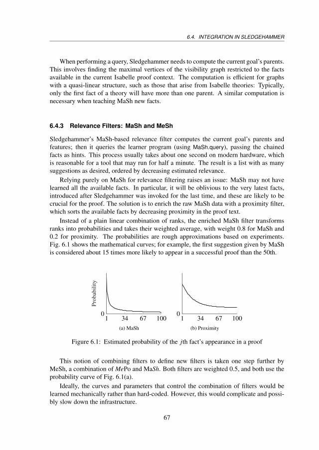
6.4. INTEGRATION IN SLEDGEHAMMER
When performing a query, Sledgehammer needs to compute the current goal’s parents.This involves finding the maximal vertices of the visibility graph restricted to the factsavailable in the current Isabelle proof context. The computation is efficient for graphswith a quasi-linear structure, such as those that arise from Isabelle theories: Typically,only the first fact of a theory will have more than one parent. A similar computation isnecessary when teaching MaSh new facts.
6.4.3 Relevance Filters: MaSh and MeSh
Sledgehammer’s MaSh-based relevance filter computes the current goal’s parents andfeatures; then it queries the learner program (using MaSh.query), passing the chainedfacts as hints. This process usually takes about one second on modern hardware, whichis reasonable for a tool that may run for half a minute. The result is a list with as manysuggestions as desired, ordered by decreasing estimated relevance.
Relying purely on MaSh for relevance filtering raises an issue: MaSh may not havelearned all the available facts. In particular, it will be oblivious to the very latest facts,introduced after Sledgehammer was invoked for the last time, and these are likely to becrucial for the proof. The solution is to enrich the raw MaSh data with a proximity filter,which sorts the available facts by decreasing proximity in the proof text.
Instead of a plain linear combination of ranks, the enriched MaSh filter transformsranks into probabilities and takes their weighted average, with weight 0.8 for MaSh and0.2 for proximity. The probabilities are rough approximations based on experiments.Fig. 6.1 shows the mathematical curves; for example, the first suggestion given by MaShis considered about 15 times more likely to appear in a successful proof than the 50th.
1 34 67 1000
Prob
abili
ty
(a) MaSh
1 34 67 1000
Prob
abili
ty
(b) Proximity
Figure 6.1: Estimated probability of the jth fact’s appearance in a proof
This notion of combining filters to define new filters is taken one step further byMeSh, a combination of MePo and MaSh. Both filters are weighted 0.5, and both use theprobability curve of Fig. 6.1(a).
Ideally, the curves and parameters that control the combination of filters would belearned mechanically rather than hard-coded. However, this would complicate and possi-bly slow down the infrastructure.
67
CHAPTER 6. MASH - MACHINE LEARNING FOR SLEDGEHAMMER
6.4.4 Automatic and Manual Control
All MaSh-related activities take place as a result of a Sledgehammer invocation. WhenSledgehammer is launched, it checks whether any new facts, unknown to the visibilitygraph, are available. If so, it launches a thread to learn from their Isar proofs and updatethe graph. The first time, it may take about 10 s to learn all the facts in the backgroundtheories (assuming about 10 000 facts). Subsequent invocations are much faster.
If an automated prover succeeds, the proof is immediately taught to MaSh (usingMaSh.learn). The discharged (sub)goal may have been only one step in an unstructuredproof, in which case it has no name. Sledgehammer invents a fresh, invisible name for it.Although this anonymous goal cannot be used to prove other goals, MaSh benefits fromlearning the connection between the formula’s features and its proof.
For users who feel the need for more control, there is an unlearn command that resetsMaSh’s persistent state (using MaSh.unlearn); a learn_isar command that learns from theIsar proofs of all available facts; and a learn_prover command that invokes an automatedprover on all available facts, replacing the Isar proofs with successful ATP-generatedproofs whenever possible.
6.4.5 Nonmonotonic Theory Changes
MaSh’s model assumes that the set of facts and the visibility graph grow monotonically.One concern that arises when deploying machine learning—as opposed to evaluating itsperformance on static benchmarks—is that theories evolve nonmonotonically over time.It is left to the architecture around MaSh to recover from such changes. The followingscenarios were considered:
• A fact is deleted. The fact is kept in MaSh’s visibility graph but is silently ignoredby Sledgehammer whenever it is suggested by MaSh.
• A fact is renamed. Sledgehammer perceives this as the deletion of a fact and theaddition of another (identical) fact.
• A theory is renamed. Since theory names are encoded in fact names, renaming atheory amounts to renaming all its facts.
• Two facts are reordered. The visibility graph loses synchronization with reality.Sledgehammer may need to ignore a suggestion because it appears to be visibleaccording to the graph.
• A fact is introduced between two facts φ and φ′. MaSh offers no facility to changethe parent of φ′, but this is not needed. By making the new fact a child of φ, it isconsidered during the computation of maximal vertices and hence visible.
• The fact’s formula is modified. This occurs when users change the statement of alemma, but also when they rename or relocate a symbol. MaSh is not informed ofsuch changes and may lose some of its predictive power.
68
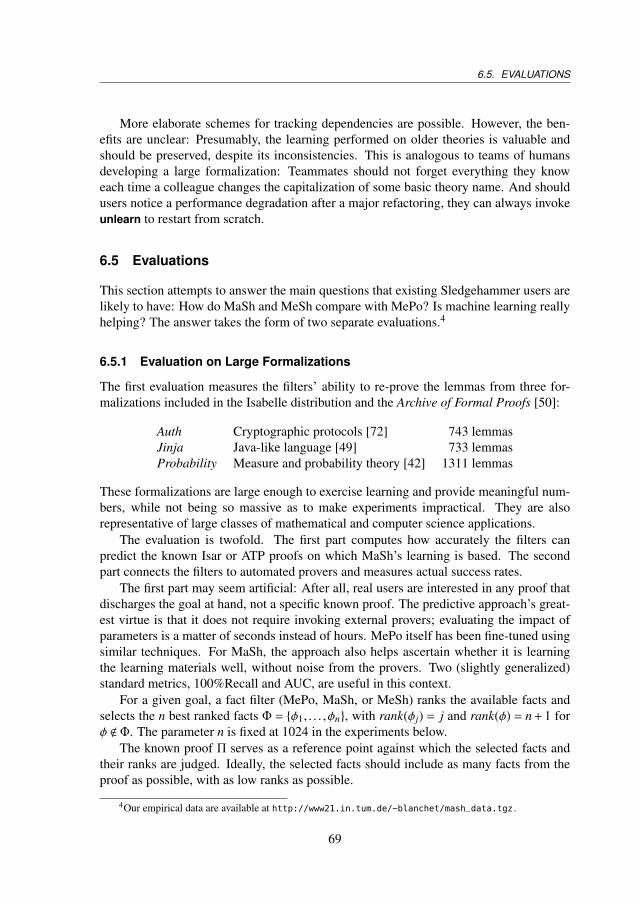
6.5. EVALUATIONS
More elaborate schemes for tracking dependencies are possible. However, the ben-efits are unclear: Presumably, the learning performed on older theories is valuable andshould be preserved, despite its inconsistencies. This is analogous to teams of humansdeveloping a large formalization: Teammates should not forget everything they knoweach time a colleague changes the capitalization of some basic theory name. And shouldusers notice a performance degradation after a major refactoring, they can always invokeunlearn to restart from scratch.
6.5 Evaluations
This section attempts to answer the main questions that existing Sledgehammer users arelikely to have: How do MaSh and MeSh compare with MePo? Is machine learning reallyhelping? The answer takes the form of two separate evaluations.4
6.5.1 Evaluation on Large Formalizations
The first evaluation measures the filters’ ability to re-prove the lemmas from three for-malizations included in the Isabelle distribution and the Archive of Formal Proofs [50]:
Auth Cryptographic protocols [72] 743 lemmasJinja Java-like language [49] 733 lemmasProbability Measure and probability theory [42] 1311 lemmas
These formalizations are large enough to exercise learning and provide meaningful num-bers, while not being so massive as to make experiments impractical. They are alsorepresentative of large classes of mathematical and computer science applications.
The evaluation is twofold. The first part computes how accurately the filters canpredict the known Isar or ATP proofs on which MaSh’s learning is based. The secondpart connects the filters to automated provers and measures actual success rates.
The first part may seem artificial: After all, real users are interested in any proof thatdischarges the goal at hand, not a specific known proof. The predictive approach’s great-est virtue is that it does not require invoking external provers; evaluating the impact ofparameters is a matter of seconds instead of hours. MePo itself has been fine-tuned usingsimilar techniques. For MaSh, the approach also helps ascertain whether it is learningthe learning materials well, without noise from the provers. Two (slightly generalized)standard metrics, 100%Recall and AUC, are useful in this context.
For a given goal, a fact filter (MePo, MaSh, or MeSh) ranks the available facts andselects the n best ranked facts Φ = {φ1, . . . ,φn}, with rank(φj) = j and rank(φ) = n + 1 forφ < Φ. The parameter n is fixed at 1024 in the experiments below.
The known proof Π serves as a reference point against which the selected facts andtheir ranks are judged. Ideally, the selected facts should include as many facts from theproof as possible, with as low ranks as possible.
4Our empirical data are available at http://www21.in.tum.de/~blanchet/mash_data.tgz .
69
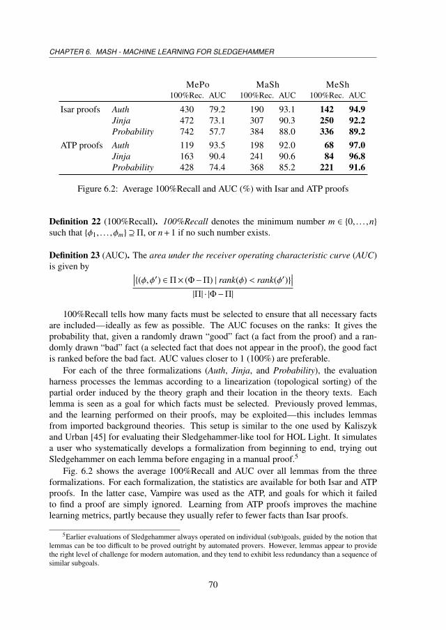
CHAPTER 6. MASH - MACHINE LEARNING FOR SLEDGEHAMMER
MePo MaSh MeSh100%Rec. AUC 100%Rec. AUC 100%Rec. AUC
Isar proofs Auth 430 79.2 190 93.1 142 94.9Jinja 472 73.1 307 90.3 250 92.2Probability 742 57.7 384 88.0 336 89.2
ATP proofs Auth 119 93.5 198 92.0 68 97.0Jinja 163 90.4 241 90.6 84 96.8Probability 428 74.4 368 85.2 221 91.6
Figure 6.2: Average 100%Recall and AUC (%) with Isar and ATP proofs
Definition 22 (100%Recall). 100%Recall denotes the minimum number m ∈ {0, . . . ,n}such that {φ1, . . . ,φm} ⊇ Π, or n + 1 if no such number exists.
Definition 23 (AUC). The area under the receiver operating characteristic curve (AUC)is given by ∣∣∣{(φ,φ′) ∈ Π× (Φ−Π) | rank(φ) < rank(φ′)}
∣∣∣|Π| · |Φ−Π|
100%Recall tells how many facts must be selected to ensure that all necessary factsare included—ideally as few as possible. The AUC focuses on the ranks: It gives theprobability that, given a randomly drawn “good” fact (a fact from the proof) and a ran-domly drawn “bad” fact (a selected fact that does not appear in the proof), the good factis ranked before the bad fact. AUC values closer to 1 (100%) are preferable.
For each of the three formalizations (Auth, Jinja, and Probability), the evaluationharness processes the lemmas according to a linearization (topological sorting) of thepartial order induced by the theory graph and their location in the theory texts. Eachlemma is seen as a goal for which facts must be selected. Previously proved lemmas,and the learning performed on their proofs, may be exploited—this includes lemmasfrom imported background theories. This setup is similar to the one used by Kaliszykand Urban [45] for evaluating their Sledgehammer-like tool for HOL Light. It simulatesa user who systematically develops a formalization from beginning to end, trying outSledgehammer on each lemma before engaging in a manual proof.5
Fig. 6.2 shows the average 100%Recall and AUC over all lemmas from the threeformalizations. For each formalization, the statistics are available for both Isar and ATPproofs. In the latter case, Vampire was used as the ATP, and goals for which it failedto find a proof are simply ignored. Learning from ATP proofs improves the machinelearning metrics, partly because they usually refer to fewer facts than Isar proofs.
5Earlier evaluations of Sledgehammer always operated on individual (sub)goals, guided by the notion thatlemmas can be too difficult to be proved outright by automated provers. However, lemmas appear to providethe right level of challenge for modern automation, and they tend to exhibit less redundancy than a sequence ofsimilar subgoals.
70
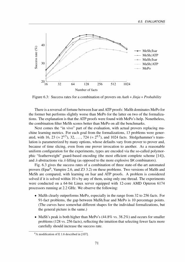
6.5. EVALUATIONS
16 32 64 128 256 512 102420
30
40
Number of facts
Succ
ess
rate
(%)
MeSh /IsarMeSh /ATPMaSh /IsarMaSh /ATPMePo
Figure 6.3: Success rates for a combination of provers on Auth + Jinja + Probability
There is a reversal of fortune between Isar and ATP proofs: MaSh dominates MePo forthe former but performs slightly worse than MePo for the latter on two of the formaliza-tions. The explanation is that the ATP proofs were found with MePo’s help. Nonetheless,the combination filter MeSh scores better than MePo on all the benchmarks.
Next comes the “in vivo” part of the evaluation, with actual provers replacing ma-chine learning metrics. For each goal from the formalizations, 13 problems were gener-ated, with 16, 23 (≈ 24.5), 32, . . . , 724 (≈ 29.5), and 1024 facts. Sledgehammer’s trans-lation is parameterized by many options, whose defaults vary from prover to prover and,because of time slicing, even from one prover invocation to another. As a reasonableuniform configuration for the experiments, types are encoded via the so-called polymor-phic “featherweight” guard-based encoding (the most efficient complete scheme [14]),and λ-abstractions via λ-lifting (as opposed to the more explosive SK combinators).
Fig. 6.3 gives the success rates of a combination of three state-of-the-art automatedprovers (Epar6, Vampire 2.6, and Z3 3.2) on these problems. Two versions of MaSh andMeSh are compared, with learning on Isar and ATP proofs. A problem is consideredsolved if it is solved within 10 s by any of them, using only one thread. The experimentswere conducted on a 64-bit Linux server equipped with 12-core AMD Opteron 6174processors running at 2.2 GHz. We observe the following:
• MaSh clearly outperforms MePo, especially in the range from 32 to 256 facts. For91-fact problems, the gap between MaSh /Isar and MePo is 10 percentage points.(The curves have somewhat different shapes for the individual formalizations, butthe general picture is the same.)
• MaSh’s peak is both higher than MePo’s (44.8% vs. 38.2%) and occurs for smallerproblems (128 vs. 256 facts), reflecting the intuition that selecting fewer facts morecarefully should increase the success rate.
6A modification of E 1.6 described in [107].
71
CHAPTER 6. MASH - MACHINE LEARNING FOR SLEDGEHAMMER
MePo MaSh MeSh
E 55.0 49.8 56.6SPASS 57.2 49.1 57.7Vampire 55.3 49.7 56.0Z3 53.0 51.8 60.8Together 65.6 63.0 69.8
Figure 6.4: Success rates (%) on Judgment Day goals
• MeSh adds a few percentage points to MaSh. The effect is especially marked forthe problems with fewer facts.
• Against expectations, learning from ATP proofs has a negative impact. A closerinspection of the raw data revealed that Vampire performs better with ATP (i.e.,Vampire) proofs, whereas the other two provers prefer Isar proofs.
Another measure of MaSh and MeSh’s power is the total number of goals solved forany number of facts. With MePo alone, 46.3% of the goals are solved; adding MaShand MeSh increases this figure to 62.7%. Remarkably, for Probability—the most difficultformalization by any standard—the corresponding figures are 27.1% vs. 47.2%.
6.5.2 Judgment Day
The Judgment Day benchmarks [20] consist of 1268 interactive goals arising in sevenIsabelle theories, covering among them areas as diverse as the fundamental theorem ofalgebra, the completeness of a Hoare logic, and Jinja’s type soundness. The evaluationharness invokes Sledgehammer on each goal. The same hardware is used as in the originalJudgment Day study [20]: 32-bit Linux servers with Intel Xeon processors running at3.06 GHz. The time limit is 60 s for proof search, potentially followed by minimizationand reconstruction in Isabelle. MaSh is trained on 9852 Isar proofs from the backgroundlibraries imported by the seven theories under evaluation.
The comparison comprises E 1.6, SPASS 3.8ds, Vampire 2.6, and Z3 3.2, whichSledgehammer employs by default. Each prover is invoked with its own options andproblems, including prover-specific features (e.g., arithmetic for Z3; sorts for SPASS,Vampire, and Z3). Time slicing is enabled. For MeSh, some of the slices use MePo orMaSh directly to promote complementarity.
The results are summarized in Fig. 6.4. Again, MeSh performs very well: The overall4.2 percentage point gain, from 65.6% to 69.8%, is highly significant. As noted in asimilar study, “When analyzing enhancements to automated provers, it is important toremember what difference a modest-looking gain of a few percentage points can make tousers” [17, §7]. Incidentally, the 65.6% score for MePo reveals progress in the underlyingprovers compared with the 63.6% figure from one year ago.
72
6.6. RELATED WORK AND CONTRIBUTIONS
The other main observation is that MaSh underperforms, especially in the light ofthe evaluation of Section 6.5.1. There are many plausible explanations. First, JudgmentDay consists of smaller theories relying on basic background theories, giving few op-portunities for learning. Consider the theory NS_Shared (Needham–Shroeder shared-keyprotocol), which is part of both evaluations. In the first evaluation, the linear progressthrough all Auth theories means that the learning performed on other, independent pro-tocols (certified email, four versions of Kerberos, and Needham–Shroeder public key)can be exploited. Second, the Sledgehammer setup has been tuned for Judgment Dayand MePo over the years (in the hope that improvements on this representative bench-mark suite would translate in improvements on users’ theories), and conversely MePo’sparameters are tuned for Judgment Day.
In future work, we want to investigate MaSh’s mediocre performance on these bench-marks (and MeSh’s remarkable results given the circumstances). The evaluation of Sec-tion 6.5.1 suggests that there are more percentage points to be gained.
6.6 Related Work and Contributions
The main related work is already mentioned in the introduction. Bridges such as Sledge-hammer for Isabelle/HOL, MizAR [109] for Mizar, and HOL(y)Hammer [45] for HOLLight are opening large formal theories to methods that combine ATPs and artificial intel-ligence (AI) [106, 57] to help automate interactive proofs. Today such large theories arethe main resource for combining semantic and statistical AI methods [111].7
The main contribution of this work has been to take the emerging machine learningmethods for fact selection and make them incremental, fast, and robust enough so thatthey run unnoticed on a single-user machine and respond well to common user-interactionscenarios. The advising services for Mizar and HOL Light [104, 103, 45, 109] (with thepartial exception of MoMM [103]) run only as remote servers trained on the main centrallibrary, and their solution to changes in the library is to ignore them or relearn everythingfrom scratch. Other novelties of this work include the use of more proof-related featuresin the learning (inspired by MePo), experiments combining MePo and MaSh, and therelated learning of various parameters of the systems involved.
6.7 Conclusion
Relevance filtering is an important practical problem that arises with large-theory rea-soning. Sledgehammer’s MaSh filter brings the benefits of machine learning methods toIsabelle users: By decreasing the quantity and increasing the quality of facts passed to theautomated provers, it helps them find more, deeper proofs within the allotted time. Thecore machine learning functionality is implemented in a separate Python program that canbe reused by other proof assistants.
7It is hard to envisage all possible combinations, but with the recent progress in natural language processing,suitable ATP/AI methods could soon be applied to another major aspect of formalization: the translation frominformal prose to formal specification.
73
CHAPTER 6. MASH - MACHINE LEARNING FOR SLEDGEHAMMER
Many areas are calling for more engineering and research; we mentioned a few al-ready. Learning data could be shared on a server or supplied with the proof assistant.More advanced algorithms appear too slow for interactive use, but they could be opti-mized. Learning could be applied to control more aspects of Sledgehammer, such as theprover options or even MePo’s parameters. Evaluations over the entire Archive of FormalProofs might shed more light on MaSh’s and MePo’s strengths and weaknesses.
Machine learning being a gift that keeps on giving, it would be fascinating to instru-ment a user’s installation to monitor performance over several months.
74
Chapter 7
MaLeS - Machine Learning of Strategies
MaLeS is a framework that develops strategies for automated theorem provers (ATPs) andcreates suitable schedules of strategies for individual problems. The framework can beused in a push-button way to develop such strategies and schedules for an arbitrary ATP.This chapter describes the tool and the methods used in it, and evaluates its performancefor three automated theorem provers: E, LEO-II and Satallax. An evaluation on a subsetof the TPTP library problems shows that, on average, a MaLeS-tuned prover solves 8.67%more problems than the prover with its default settings.
7.1 Introduction: ATP Strategies
Automated theorem proving is a search problem. Many different approaches exist, andmost of them have parameters that can be tuned. Examples of such parameterizationsare clause weighting and selection schemes, term orderings, and sets of inference andreduction rules used. For a given ATP A, its implemented parameters form A’s parameterspace. A specific choice of parameters defines a search strategy.1 The choice of a strategycan often make the difference between finding a proof in a few milliseconds or not atall (within a reasonable time limit). This naturally leads to the question: Given a newproblem, which search strategy should be used?
Considerable attention has already been paid to this problem. Gandalf [99] pioneeredstrategy scheduling: Run several search strategies sequentially with shorter time limitsinstead of a single strategy for the whole time limit. This method is used in most currentATPs, most prominently Vampire [77]. In the SETHEO project [119], a local search al-
This chapter is based on: [53] “MaLeS: A Framework for Automatic Tuning of Automated TheoremProvers” and an extension of [58] “E-MaLeS 1.1”, published in the Proceedings of the 24th Conference onAutomated Deduction.
1 Many different names exist for these concepts. In Satallax [19] parameters are called flags, and a strategyis called a mode. Option is often used as a synonym for parameter. Configurations and configuration space areother alternative names.
75
CHAPTER 7. MALES - MACHINE LEARNING OF STRATEGIES
gorithm in the space of all strategy schedules was used to find better strategy schedules.Fuchs [31] used a nearest neighbour algorithm to determine which strategy/strategies torun. Bridge’s [18] thesis is about machine learning for search heuristic selection in ATPswith a particular focus on problem features and feature selection. In the SAT commu-nity, Satzilla [120] very successfully used machine learning to decide when to run whichSAT solver. ParamILS [44] is a general tuning framework that searches for good param-eter settings with a randomized hill climbing algorithm. BliStr [107] uses ParamILS todevelop strategies for E [84] on a large set of interrelated problems.
Despite all this work, most ATPs do not harness the methods available. Search strate-gies are often manually defined by the developer of the ATP and strategy schedules arecreated by a greedy algorithm or very simple clustering. This chapter introduces MaLeS(Machine Learning (of) Strategies), an easy-to-use learning-based framework for auto-matic tuning and configuration of ATPs. It is based on and supersedes E-MaLeS 1.0 [54]and E-MaLeS 1.1 [58]. The goal of MaLeS is to help ATP users fine-tune an ATP totheir problems and provide developers with a push-button method for finding good searchstrategies and creating strategy schedules. MaLeS is implemented in Python and has beentested with the ATPs E, LEO-II [9] and Satallax [19]. The source code is freely availableat https://code.google.com/p/males/.
7.1.1 The Strategy Selection Problem
Figure 7.1 gives an overview of the strategy selection problem. Each point in the pa-rameter space corresponds to a search strategy. Parameter spaces can be very big. Forexample, the ATP E supports over 1017 different search strategies. To simplify the strat-egy selection problem, strategy selection algorithms usually only consider a small numberof preselected strategies. There are different criteria to determine which strategies shouldbe selected. The most common ones are to pick strategies that solve a lot of problems, orare very good for a particular kind of problem.
In order to determine which strategy to use for a problem, one needs to be able tocharacterize different problem classes. This is usually done by defining a set of problemfeatures. Features must be fast to compute, but also expressive enough so that the ATPbehaves similarly on problems with similar features. The features are used to determinewhich strategy is run. Hence, the strategy selection problem consists of three subprob-lems:
1. Finding a good set of preselected strategies S.
2. Defining features F which are easy to compute (via a feature function ϕ), but alsoexpressive enough to distinguish different types of problems.
3. Determining a method which given the features of a problem creates a strategyschedule.
76
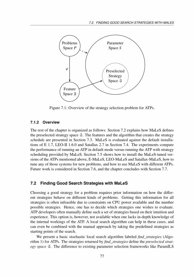
7.2. FINDING GOOD SEARCH STRATEGIES WITH MALES
ParameterSpace S
ProblemsSpace P
FeatureSpace F
PreselectedStrategySpace S
ϕ
Figure 7.1: Overview of the strategy selection problem for ATPs.
7.1.2 Overview
The rest of the chapter is organized as follows: Section 7.2 explains how MaLeS definesthe preselected strategy space S. The features and the algorithm that creates the strategyschedule are presented in Section 7.3. MaLeS is evaluated against the default installa-tions of E 1.7, LEO-II 1.6.0 and Satallax 2.7 in Section 7.4. The experiments comparethe performance of running an ATP in default mode versus running the ATP with strategyscheduling provided by MaLeS. Section 7.5 shows how to install the MaLeS-tuned ver-sions of the ATPs mentioned above, E-MaLeS, LEO-MaLeS and Satallax-MaLeS, how totune any of those systems for new problems, and how to use MaLeS with different ATPs.Future work is considered in Section 7.6, and the chapter concludes with Section 7.7.
7.2 Finding Good Search Strategies with MaLeS
Choosing a good strategy for a problem requires prior information on how the differ-ent strategies behave on different kinds of problems. Getting this information for allstrategies is often infeasible due to constraints on CPU power available and the numberpossible strategies. Hence, one has to decide which strategies one wishes to evaluate.ATP developers often manually define such a set of strategies based on their intuition andexperience. This option is, however, not available when one lacks in-depth knowledge ofthe internal workings of the ATP. A local search algorithm can help in these cases, andcan even be combined with the manual approach by taking the predefined strategies asstarting points of the search.
We present a basic stochastic local search algorithm labeled find_strategies (Algo-rithm 1) for ATPs. The strategies returned by find_strategies define the preselected strat-egy space S. The difference to existing parameter selection frameworks like ParamILS
77
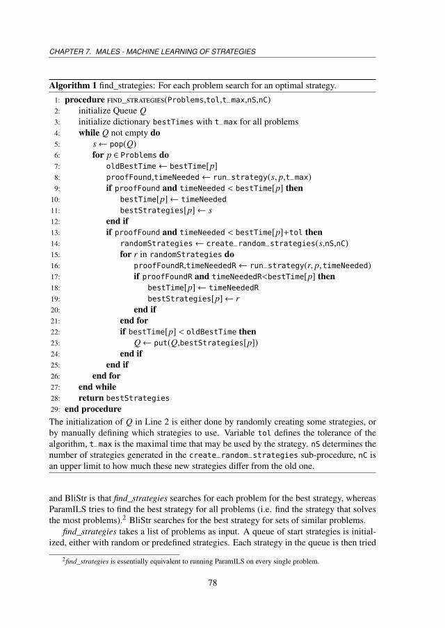
CHAPTER 7. MALES - MACHINE LEARNING OF STRATEGIES
Algorithm 1 find_strategies: For each problem search for an optimal strategy.
1: procedure find_strategies(Problems,tol,t_max,nS,nC)2: initialize Queue Q3: initialize dictionary bestTimes with t_max for all problems4: while Q not empty do5: s← pop(Q)6: for p ∈ Problems do7: oldBestTime← bestTime[p]8: proofFound,timeNeeded← run_strategy(s, p,t_max)9: if proofFound and timeNeeded < bestTime[p] then
10: bestTime[p]← timeNeeded
11: bestStrategies[p]← s12: end if13: if proofFound and timeNeeded < bestTime[p]+tol then14: randomStrategies← create_random_strategies(s,nS,nC)15: for r in randomStrategies do16: proofFoundR,timeNeededR← run_strategy(r, p,timeNeeded)17: if proofFoundR and timeNeededR<bestTime[p] then18: bestTime[p]← timeNeededR
19: bestStrategies[p]← r20: end if21: end for22: if bestTime[p] < oldBestTime then23: Q← put(Q,bestStrategies[p])24: end if25: end if26: end for27: end while28: return bestStrategies
29: end procedureThe initialization of Q in Line 2 is either done by randomly creating some strategies, orby manually defining which strategies to use. Variable tol defines the tolerance of thealgorithm, t_max is the maximal time that may be used by the strategy. nS determines thenumber of strategies generated in the create_random_strategies sub-procedure, nC isan upper limit to how much these new strategies differ from the old one.
and BliStr is that find_strategies searches for each problem for the best strategy, whereasParamILS tries to find the best strategy for all problems (i.e. find the strategy that solvesthe most problems).2 BliStr searches for the best strategy for sets of similar problems.
find_strategies takes a list of problems as input. A queue of start strategies is initial-ized, either with random or predefined strategies. Each strategy in the queue is then tried
2find_strategies is essentially equivalent to running ParamILS on every single problem.
78
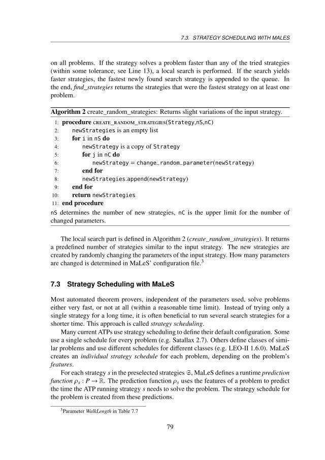
7.3. STRATEGY SCHEDULING WITH MALES
on all problems. If the strategy solves a problem faster than any of the tried strategies(within some tolerance, see Line 13), a local search is performed. If the search yieldsfaster strategies, the fastest newly found search strategy is appended to the queue. Inthe end, find_strategies returns the strategies that were the fastest strategy on at least oneproblem.
Algorithm 2 create_random_strategies: Returns slight variations of the input strategy.
1: procedure create_random_strategies(Strategy,nS,nC)2: newStrategies is an empty list3: for i in nS do4: newStrategy is a copy of Strategy5: for j in nC do6: newStrategy = change_random_parameter(newStrategy)7: end for8: newStrategies.append(newStrategy)9: end for
10: return newStrategies
11: end procedurenS determines the number of new strategies, nC is the upper limit for the number ofchanged parameters.
The local search part is defined in Algorithm 2 (create_random_strategies). It returnsa predefined number of strategies similar to the input strategy. The new strategies arecreated by randomly changing the parameters of the input strategy. How many parametersare changed is determined in MaLeS’ configuration file.3
7.3 Strategy Scheduling with MaLeS
Most automated theorem provers, independent of the parameters used, solve problemseither very fast, or not at all (within a reasonable time limit). Instead of trying only asingle strategy for a long time, it is often beneficial to run several search strategies for ashorter time. This approach is called strategy scheduling.
Many current ATPs use strategy scheduling to define their default configuration. Someuse a single schedule for every problem (e.g. Satallax 2.7). Others define classes of simi-lar problems and use different schedules for different classes (e.g. LEO-II 1.6.0). MaLeScreates an individual strategy schedule for each problem, depending on the problem’sfeatures.
For each strategy s in the preselected strategiesS, MaLeS defines a runtime predictionfunction ρs : P→ R. The prediction function ρs uses the features of a problem to predictthe time the ATP running strategy s needs to solve the problem. The strategy schedule forthe problem is created from these predictions.
3Parameter WalkLength in Table 7.7
79
CHAPTER 7. MALES - MACHINE LEARNING OF STRATEGIES
7.3.1 Notation
For the remainder of the chapter, we shall use the following notation:
• p is an ATP problem. P denotes a set of problems.
• Ptrain ⊆ P is a set of training problems that is used to tune the learning algorithm.
• F is the feature space. We assume that F is a subset of Rn for some n ∈ N.
• ϕ : P→ F is the feature function. ϕ(p) is the feature vector of a problem.
• S is the parameter space, S is the set of preselected strategies.
• The time the ATP running strategy s needs to solve a problem p is denoted byτ(p, s). If s is obvious from the context or irrelevant, we also use τ(p).
• For a strategy s, ρs : P→ R is the runtime prediction function.
7.3.2 Features
Features give an abstract description of a problem. Optimally, the features should be de-signed in such a way that the ATP behaves similar on problems with similar features, i.e.if two problem p,q have similar features ϕ(p)∼ ϕ(q), then for each strategy s the runtimesshould be similar τ(p, s) ∼ τ(q, s). The similarity function (e.g. cosine distance betweenthe feature vectors) and set of features heavily influence the quality of the predictionfunctions. Indeed, feature selection is an entire subfield of machine learning [59, 36].
Currently, MaLeS supports two different feature spaces: Schulz’s E features are usedfor first order (FOF) problems. The TPTP features designed by Sutcliffe are used forhigher order (THF) problems [96].
The E Features
Schulz designed a set of features for clause-normal-form and first order problems. Theyare used in the strategy selection process in his theorem prover E [58]. Table 7.1 shows thefeatures together with a short description.4 MaLeS uses the same features for first-orderproblems. A clause is called negative if it only has negative literals. It is called positive ifit only has positive literals. A ground clause is a clause that contains no variables. In thissetting, we refer to all negative clauses as “goals”, and to all other clauses as “axioms".Clauses can be unit (having only a single literal), Horn (having at most one positiveliteral), or general (no constraints on the form). All unit clauses are Horn, and all Hornclauses are general.
The features are computed by running Schulz’s classify_problem program which isdistributed with MaLeS.
4The author would like to thank Stephan Schulz for the design of the features, the program that extractsthem and their precise description in this subsection.
80
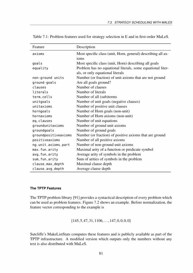
7.3. STRATEGY SCHEDULING WITH MALES
Table 7.1: Problem features used for strategy selection in E and in first-order MaLeS.
Feature Description
axioms Most specific class (unit, Horn, general) describing all ax-ioms
goals Most specific class (unit, Horn) describing all goalsequality Problem has no equational literals, some equational liter-
als, or only equational literalsnon-ground units Number (or fraction) of unit axioms that are not groundground-goals Are all goals ground?clauses Number of clausesliterals Number of literalsterm_cells Number of all (sub)termsunitgoals Number of unit goals (negative clauses)unitaxioms Number of positive unit clauseshorngoals Number of Horn goals (non-unit)hornaxioms Number of Horn axioms (non-unit)eq_clauses Number of unit equationsgroundunitaxioms Number of ground unit axiomsgroundgoals Number of ground goalsgroundpositiveaxioms Number (or fraction) of positive axioms that are groundpositiveaxioms Number of all positive axiomsng_unit_axioms_part Number of non-ground unit axiomsmax_fun_arity Maximal arity of a function or predicate symbolavg_fun_arity Average arity of symbols in the problemsum_fun_arity Sum of arities of symbols in the problemclause_max_depth Maximal clause depthclause_avg_depth Average clause depth
The TPTP Features
The TPTP problem library [91] provides a syntactical description of every problem whichcan be used as problem features. Figure 7.2 shows an example. Before normalization, thefeature vector corresponding to the example is
[145,5,47,31,1106, . . . ,147,0,0,0,0]
Sutcliffe’s MakeListStats computes these features and is publicly available as part of theTPTP infrastructure. A modified version which outputs only the numbers without anytext is also distributed with MaLeS.
81
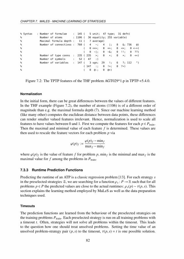
CHAPTER 7. MALES - MACHINE LEARNING OF STRATEGIES
% Syntax : Number of formulae : 145 ( 5 unit; 47 type; 31 defn)% Number of atoms : 1106 ( 36 equality; 255 variable)% Maximal formula depth : 11 ( 7 average)% Number of connectives : 760 ( 4 ~; 4 |; 8 &; 736 @)% ( 0 <=>; 8 =>; 0 <=; 0 <~>)% ( 0 ~|; 0 ~&; 0 !!; 0 ??)% Number of type conns : 235 ( 235 >; 0 *; 0 +; 0 <<)% Number of symbols : 52 ( 47 :)% Number of variables : 147 ( 3 sgn; 29 !; 6 ?; 112 ^)% ( 147 :; 0 !>; 0 ?*)% ( 0 @-; 0 @+)
Figure 7.2: The TPTP features of the THF problem AGT029^1.p in TPTP-v5.4.0.
Normalization
In the initial form, there can be great differences between the values of different features.In the THF example (Figure 7.2), the number of atoms (1106) is of a different order ofmagnitude than e.g. the maximal formula depth (7). Since our machine learning method(like many other) computes the euclidean distance between data points, these differencescan render smaller valued features irrelevant. Hence, normalization is used to scale allfeatures to have values between 0 and 1. First we compute the features for each p ∈ Ptrain.Then the maximal and minimal value of each feature f is determined. These values arethen used to rescale the feature vectors for each problem p via
ϕ(p) f :=ϕ(p) f −min f
max f −min f
where ϕ(p) f is the value of feature f for problem p, min f is the minimal and max f is themaximal value for f among the problems in Ptrain.
7.3.3 Runtime Prediction Functions
Predicting the runtime of an ATP is a classic regression problem [13]. For each strategy sin the preselected strategiesS, we are searching for a function ρs : P→R such that for allproblems p ∈ P the predicted values are close to the actual runtimes: ρs(p) ∼ τ(p, s). Thissection explains the learning method employed by MaLeS as well as the data preparationtechniques used.
Timeouts
The prediction functions are learned from the behaviour of the preselected strategies onthe training problems Ptrain. Each preselected strategy is run on all training problems witha timeout t. Often, strategies will not solve all problems within the timeout. This leadsto the question how one should treat unsolved problems. Setting the time value of anunsolved problem-strategy pair (p, s) to the timeout, τ(p, s) = t is one possible solution.
82
7.3. STRATEGY SCHEDULING WITH MALES
Another possibility, which is used in MaLeS, is to only learn on problems that can besolved. While ignoring unsolved problems introduces a bias towards shorter runtimes, italso simplifies the computation of the prediction functions and allows us to update theprediction functions at runtime (Section 7.3.5). If MaLeS runs the ATP with strategy sfor a time limit t on a problem p and the ATP does not find a solution, then MaLeS usesthis information to update the prediction functions and adapt the strategy schedule for pat runtime.
Kernel Methods
MaLeS uses kernels to learn the runtime prediction function. Kernels are a very popularmachine learning method that has successfully been applied in many domains [88]. Akernel can be seen as a similarity function between feature vectors. Kernels allow theusage of nonlinear features while keeping the learning problem itself linear. The basicprinciples will be covered on the next pages. More information about kernel-based ma-chine learning can be found in [88].
Definition 24 (Gaussian Kernel). The Gaussian kernel k with parameter σ of two prob-lems p,q ∈ P with feature vectors ϕ(p),ϕ(q) ∈ F ⊆ Rn for some n ∈ N is defined as
k(p,q) := exp(−ϕ(p)Tϕ(p)−2ϕ(p)Tϕ(q) +ϕ(q)Tϕ(q)
σ2
)ϕ(p)T is the transposed vector, and hence ϕ(p)Tϕ(q) is the dot product between ϕ(p) andϕ(q) in Rn.
In order to apply machine learning, we first need some data to learn from. Let t ∈R bea time limit. For each preselected strategy s ∈S, the ATP is run with strategy s and timelimit t on each problem in Ptrain. For each strategy s, Ps
train ⊆ Ptrain is the set of problemsthat the ATP can solve within the time limit t with strategy s. In kernel based machinelearning, the prediction function ρs has the form
ρs(p) =∑
q∈Pstrain
αsqk(p,q)
for some αsq ∈ R. The αs
q are called weights and are the result of the learning. To definehow exactly this is done, some more notation is needed.
Definition 25 (Kernel Matrix, Times Matrix and Weights Matrix). For every strategys ∈ S, let m be the number of problems in Ps
train and (pi)i∈m be an enumeration of theproblems in Ps
train. The kernel matrix K s ∈ Rm×m is defined as
K si, j := k(pi, p j)
We define the time matrix Y s ∈ R1×m via
Y si := τ(pi, s)
83
CHAPTER 7. MALES - MACHINE LEARNING OF STRATEGIES
Finally, we set the weight matrix As ∈ Rm×1 as
Asi := αs
pi
If is it obvious which strategy is meant, or the statement is independent of the strategy,we omit the s in K s,Y s and As.
A simple way to define A would be to solve KA = Y . Such a solution (if it exists)would likely perform very well on known data but poorly on new data, a behaviour calledoverfitting. A regularization parameter λ ∈ R is added as a penalty for complex predic-tion functions. Least square regression is used to minimize the difference between thepredicted times and the actual times [78]. That means we want
A = argminA∈Rm×1
((Y −KA)T (Y −KA) +λAT KA
)The first part of the equation (Y −KA)T (Y −KA) is the square loss between the predictedvalues and the actual time needed. λAT KA is the regularization term. The bigger λ, themore complex functions are penalized [78]. For very high values of λ, we force A to bealmost equal to the 0 matrix. This approach can be seen as a kind of Occam’s razor forprediction functions. A is the matrix that best fits the training data while staying as simpleas possible.
Theorem 1 (Weight Matrix for a Strategy). For λ > 0, the optimal weights for a strategys are given by
A = (K +λI)−1Y
with I being the identity matrix in Rm×m.
Proof.
∂∂A
((Y −KA)T(Y −KA) +λATKA
)= −2K(Y −KA) + 2λKA
= −2KY + (2KK + 2λK)A
It can be shown that K is a positive-semi definite symmetric matrix and therefore (K +λI)is invertible for λ > 0. To find a minimum, we set the derivative to zero and solve withrespect to A.
K(K +λI)A = KY
and hence
A = (K +λI)−1Y
is a solution. �
84
7.3. STRATEGY SCHEDULING WITH MALES
7.3.4 Crossvalidation
Finally, the values for the regularization constant λ and the kernel width σ need to bedetermined. This is done via 10-fold cross-validation on the training problems, a standardmachine learning method for such tasks [51]. Cross-validation simulates the effect ofnot knowing the data and picks the values that perform, in general, best on unknownproblems.
First a finite number of possible values for λ and σ is defined. Then, the trainingset Ps
train is split in 10 disjoint, equally sized subsets P1, . . .P10. For all 1 ≤ i ≤ 10, eachpossible combination of values for λ and σ is trained on Ps
train −Pi and evaluated on Pi.The evaluation is done by computing the square-loss between the predicted runtimes andthe actual runtimes. The combination with the least average square loss is used.
7.3.5 Creating Schedules from Prediction Functions
Having defined the prediction functions, we can now introduce the scheduling algorithmthat is used when trying to solve new problem. For each new problem, MaLeS uses theprediction functions to select the strategy and runtime that is most likely (according toour model) to solve the problem. If the predicted strategy does not solve the problem,MaLeS updates all prediction functions with this new information. Algorithm 3 showsthe details.
In line 2 the algorithm starts by running some predefined start strategies. The goal ofrunning these start strategies first is to filter out simple problems which allows the learningalgorithm to focus on the harder problems. The start strategies are picked greedily. Firstthe strategy that solves most problems (within some time limit) is chosen. Then thestrategy that solves most of the problems that were not solved by the first picked strategy(within some time limit) is picked, etc. The number of start strategies and their runtimeare determined via their respective parameters in the setup.ini file (Table 7.8). Trainingproblems that are solved by the start strategies are deleted from the training set. Forexample, let s1, . . . , sn be the starting strategies, all with a runtime of 1 second. Then forall s ∈ S ′ we can set
Pstrain := {p ∈ Ps
train | ∀ 1 ≤ i ≤ n τ(p, si) > 1}
and train ρs on the updated Pstrain.
The subprocedure choose_best_strategy in line 12 picks the strategy with the mini-mum predicted runtime among those that have not been run with a bigger or equal runtimebefore.5 run_strategy runs the ATP with strategy s′ and time limit ts′ on the problem.If the ATP cannot solve the problem within the time limit, this information is used toimprove the prediction functions in update_prediction_function (Line 19). For this,all the training problems that are solved by the picked strategy s′ within the predictedruntime ts′ are deleted from the training set Ptrain, i.e. for all s ∈ S ′
Pstrain := {p ∈ Ps
train | τ(p, s′) > ts′ }
5If there are several strategies with the same minimal predicted runtime a random one is chosen.
85
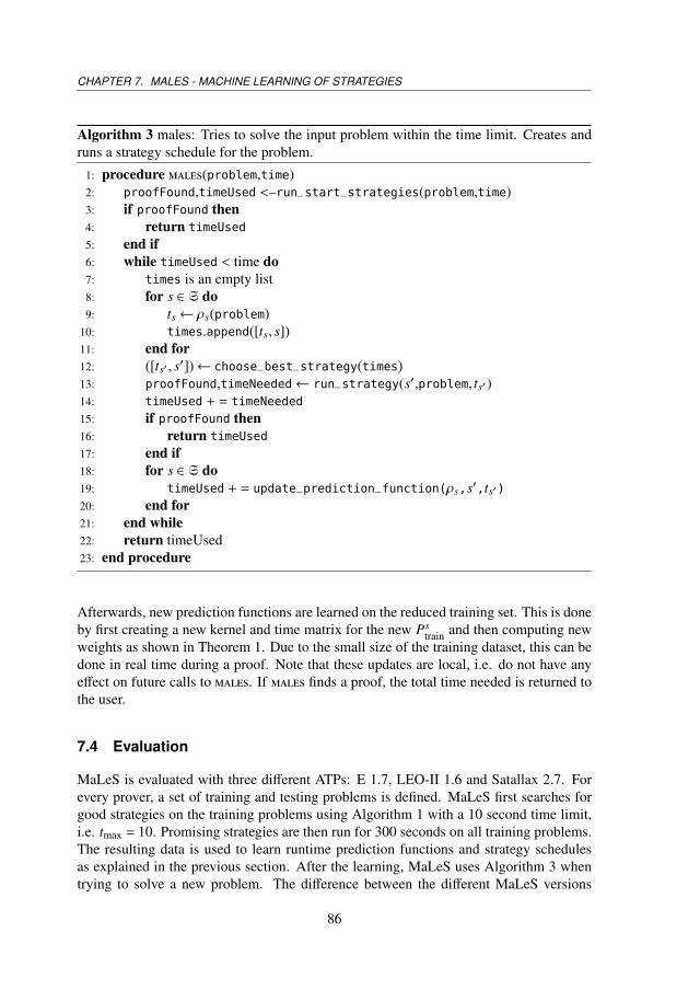
CHAPTER 7. MALES - MACHINE LEARNING OF STRATEGIES
Algorithm 3 males: Tries to solve the input problem within the time limit. Creates andruns a strategy schedule for the problem.
1: procedure males(problem,time)2: proofFound,timeUsed <–run_start_strategies(problem,time)3: if proofFound then4: return timeUsed
5: end if6: while timeUsed < time do7: times is an empty list8: for s ∈S do9: ts← ρs(problem)
10: times.append([ts, s])11: end for12: ([ts′ , s′])← choose_best_strategy(times)13: proofFound,timeNeeded← run_strategy(s′,problem, ts′ )14: timeUsed + = timeNeeded
15: if proofFound then16: return timeUsed
17: end if18: for s ∈S do19: timeUsed + = update_prediction_function(ρs,s′,ts′)
20: end for21: end while22: return timeUsed23: end procedure
Afterwards, new prediction functions are learned on the reduced training set. This is doneby first creating a new kernel and time matrix for the new Ps
train and then computing newweights as shown in Theorem 1. Due to the small size of the training dataset, this can bedone in real time during a proof. Note that these updates are local, i.e. do not have anyeffect on future calls to males. If males finds a proof, the total time needed is returned tothe user.
7.4 Evaluation
MaLeS is evaluated with three different ATPs: E 1.7, LEO-II 1.6 and Satallax 2.7. Forevery prover, a set of training and testing problems is defined. MaLeS first searches forgood strategies on the training problems using Algorithm 1 with a 10 second time limit,i.e. tmax = 10. Promising strategies are then run for 300 seconds on all training problems.The resulting data is used to learn runtime prediction functions and strategy schedulesas explained in the previous section. After the learning, MaLeS uses Algorithm 3 whentrying to solve a new problem. The difference between the different MaLeS versions
86
7.4. EVALUATION
(i.e. E-MaLeS, Satallax-MaLeS and Leo-MaLeS) is the training data used to create theprediction functions and start strategies, and the ATP that is run in the run_strategy partof Algorithm 3. The MaLeS version of the ATP is compared with the default mode onboth the test and the training problems. The section ends with an overview of previousversions of MaLeS and their CASC performance.
7.4.1 E-MaLeS
E is a popular ATP for first order logic. It is open source, easily available and consistentlyperforms very well at the CASC competitions. Additionally, E is easily tunable witha big parameter space6 which suggested that parameter tuning could lead to significantimprovements. All computations were done on a 64 core AMD Opteron Processor 6276with 1.4GHz per CPU and 256 GB of RAM
E’s Automatic Mode
E’s automatic mode is developed by Stephan Schulz and based on a static partitioning ofthe set of all problems into disjoint classes. It is generated in two steps. First, the setof all training examples (typically the set of all current TPTP problems) is classified intodisjoint classes using some of the features listed in Table 7.1. For the numeric features,threshold values have originally been selected to split the TPTP into 3 or 4 approximatelyequal subsets on each feature. Over time, these have been manually adapted using trialand error.
Once the classification is fixed, a Python program reads the different classes and as-signs to each class one of the strategies that solves the most examples in this class. Forlarge classes (arbitrarily defined as having more than 200 problems), it picks the strat-egy that also is fastest on that class. For small classes, it picks the globally best strategyamong those that solve the maximum number of problems. A class with zero solutionsby all strategies is assigned the overall best strategy.
The Training Data
The problems from the FOF divisions of CASC-22 [92], CASC-J5 [93], CASC-23 [94]and CASC-J6 and CASC@Turing [95] were used as training problems. Several problemsappeared in more than one CASC. There are also a few problems from earlier CASCs thatare not part of the TPTP version used in the experiments, TPTP-v5.4.0. Deleting dupli-cates and missing problems leaves 1112 problems that were used to train E-MaLeS. Thestrategy search for the set of preselected strategies took three weeks on a 64 core server.The majority of the time was spent running promising strategies with a 300 seconds timelimit. Over 2 million strategies were considered. Of those, 109 were selected to be usedin E-MaLeS. E-MaLeS runs 10 start strategies, each with a 1 second time limit. E 1.7(running the automatic mode) and E-MaLeS were evaluated on all training problems witha 300 second time limit. The results can be seen in Figure 7.3.
6The parameter space considered in the experiments contains more than 1017 different strategies.
87
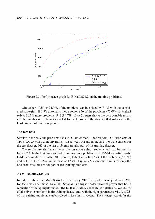
CHAPTER 7. MALES - MACHINE LEARNING OF STRATEGIES
Figure 7.3: Performance graph for E-MaLeS 1.2 on the training problems.
Altogether, 1055, or 94.9%, of the problems can be solved by E 1.7 with the consid-ered strategies. E 1.7’s automatic mode solves 856 of the problems (77.0%), E-MaLeSsolves 10.0% more problems: 942 (84.7%). Best Strategy shows the best possible result,i.e. the number of problems solved if for each problem the strategy that solves it in theleast amount of time was picked.
The Test Data
Similar to the way the problems for CASC are chosen, 1000 random FOF problems ofTPTP-v5.4.0 with a difficulty rating [98] between 0.2 and (including) 1.0 were chosen forthe test dataset. 165 of the test problems are also part of the training dataset.
The results are similar to the results on the training problems and can be seen inFigure 7.4. In the first three seconds, E solves more problems than E-MaLeS. Afterwards,E-MaLeS overtakes E. After 300 seconds, E-MaLeS solves 573 of the problems (57.3%)and E 1.7 511 (51.1%), an increase of 12.4%. Figure 7.5 shows the results for only the835 problems that are not part of the training problems.
7.4.2 Satallax-MaLeS
In order to show that MaLeS works for arbitrary ATPs, we picked a very different ATPfor the next experiment: Satallax. Satallax is a higher order theorem prover that has areputation of being highly tuned. The built-in strategy schedule of Satallax solves 95.3%of all solvable problems in the training dataset and, with the right parameters, 91.3% (525)of the training problems can be solved in less than 1 second. The strategy search for the
88

7.4. EVALUATION
Figure 7.4: Performance graph for E-MaLeS 1.2 on the test problems.
Figure 7.5: Performance graph for E-MaLeS 1.2 on the unseen test problems.
set of preselected strategies was done on a 32 core Intel Xeon with 2.6GHz per CPU and256 GB of RAM. The evaluations were done on a 64 core AMD Opteron Processor 6276with 1.4GHz per CPU and 256 GB of RAM.
89
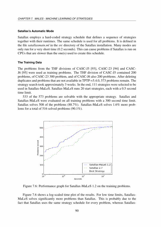
CHAPTER 7. MALES - MACHINE LEARNING OF STRATEGIES
Satallax’s Automatic Mode
Satallax employs a hard-coded strategy schedule that defines a sequence of strategiestogether with their runtimes. The same schedule is used for all problems. It is defined inthe file satallaxmain.ml in the src directory of the Satallax installation. Many modes areonly run for a very short time (0.2 seconds). This can cause problems if Satallax is run onCPUs that are slower than the one(s) used to create this schedule.
The Training Data
The problems from the THF divisions of CASC-J5 [93], CASC-23 [94] and CASC-J6 [95] were used as training problems. The THF division of CASC-J5 contained 200problems, of CASC-23 300 problem, and of CASC-J6 also 200 problems. After deletingduplicates and problems that are not available in TPTP-v5.4.0, 573 problems remain. Thestrategy search took approximately 3 weeks. In the end, 111 strategies were selected to beused in Satallax-MaLeS. Satallax-MaLeS runs 20 start strategies, each with a 0.5 secondtime limit.
533 of the 573 problems are solvable with the appropriate strategy. Satallax andSatallax-MaLeS were evaluated on all training problems with a 300 second time limit.Satallax solves 508 of the problems (88.7%). Satallax-MaLeS solves 1.6% more prob-lems for a total of 516 solved problems (90.1%).
Figure 7.6: Performance graph for Satallax-MaLeS 1.2 on the training problems.
Figure 7.6 shows a log-scaled time plot of the results. For low time limits, Satallax-MaLeS solves significantly more problems than Satallax. This is probably due to thefact that Satallax uses the same strategy schedule for every problem, whereas Satallax-
90
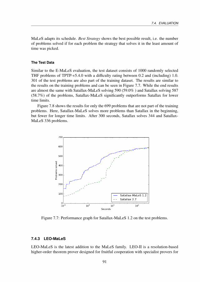
7.4. EVALUATION
MaLeS adapts its schedule. Best Strategy shows the best possible result, i.e. the numberof problems solved if for each problem the strategy that solves it in the least amount oftime was picked.
The Test Data
Similar to the E-MaLeS evaluation, the test dataset consists of 1000 randomly selectedTHF problems of TPTP-v5.4.0 with a difficulty rating between 0.2 and (including) 1.0.301 of the test problems are also part of the training dataset. The results are similar tothe results on the training problems and can be seen in Figure 7.7. While the end resultsare almost the same with Satallax-MaLeS solving 590 (59.0% ) and Satallax solving 587(58.7%) of the problems, Satallax-MaLeS significantly outperforms Satallax for lowertime limits.
Figure 7.8 shows the results for only the 699 problems that are not part of the trainingproblems. Here, Satallax-MaLeS solves more problems than Satallax in the beginning,but fewer for longer time limits. After 300 seconds, Satallax solves 344 and Satallax-MaLeS 336 problems.
Figure 7.7: Performance graph for Satallax-MaLeS 1.2 on the test problems.
7.4.3 LEO-MaLeS
LEO-MaLeS is the latest addition to the MaLeS family. LEO-II is a resolution-basedhigher-order theorem prover designed for fruitful cooperation with specialist provers for
91
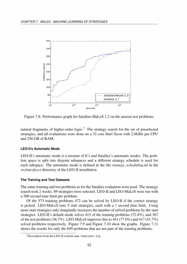
CHAPTER 7. MALES - MACHINE LEARNING OF STRATEGIES
Figure 7.8: Performance graph for Satallax-MaLeS 1.2 on the unseen test problems.
natural fragments of higher-order logic.7 The strategy search for the set of preselectedstrategies, and all evaluations were done on a 32 core Intel Xeon with 2.6GHz per CPUand 256 GB of RAM.
LEO-II’s Automatic Mode
LEO-II’s automatic mode is a mixture of E’s and Satallax’s automatic modes. The prob-lem space is split into disjoint subspaces and a different strategy schedule is used foreach subspace. The automatic mode is defined in the file strategy_scheduling.ml in thesrc/interfaces directory of the LEO-II installation.
The Training and Test Datasets
The same training and test problems as for the Satallax evaluation were used. The strategysearch took 2 weeks. 89 strategies were selected. LEO-II and LEO-MaLeS were run witha 300 second time limit per problem.
Of the 573 training problems 472 can be solved by LEO-II if the correct strategyis picked. LEO-MaLeS runs 5 start strategies, each with a 1 second time limit. Usingmore start strategies only marginally increases the number of solved problems by the startstrategies. LEO-II’s default mode solves 415 of the training problems (72.4%), and 367of the test problems (36.7%). LEO-MaLeS improves this to 441 (77.0%) and 417 (41.7%)solved problems respectively. Figure 7.9 and Figure 7.10 show the graphs. Figure 7.11shows the results for only the 699 problems that are not part of the training problems.
7Description from the LEO-II website www.leoprover.org.
92
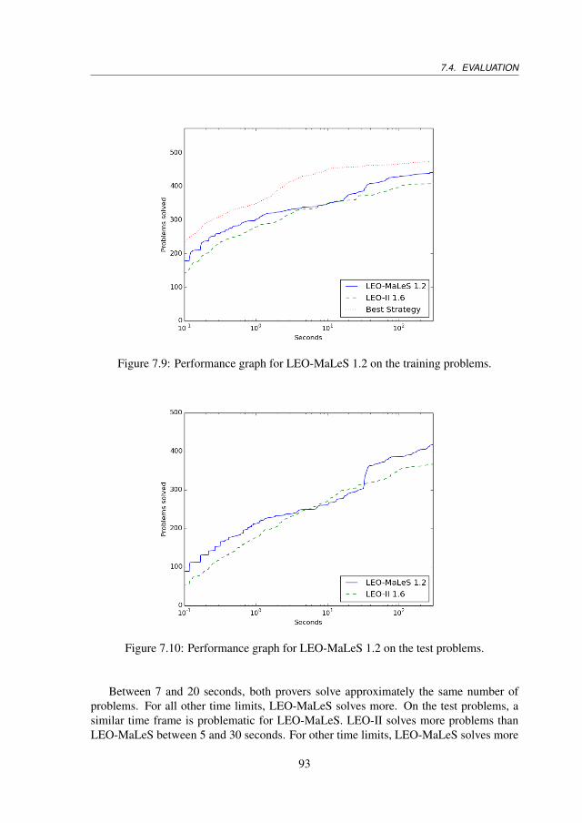
7.4. EVALUATION
Figure 7.9: Performance graph for LEO-MaLeS 1.2 on the training problems.
Figure 7.10: Performance graph for LEO-MaLeS 1.2 on the test problems.
Between 7 and 20 seconds, both provers solve approximately the same number ofproblems. For all other time limits, LEO-MaLeS solves more. On the test problems, asimilar time frame is problematic for LEO-MaLeS. LEO-II solves more problems thanLEO-MaLeS between 5 and 30 seconds. For other time limits, LEO-MaLeS solves more
93
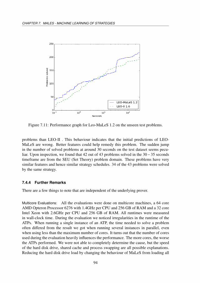
CHAPTER 7. MALES - MACHINE LEARNING OF STRATEGIES
Figure 7.11: Performance graph for Leo-MaLeS 1.2 on the unseen test problems.
problems than LEO-II . This behaviour indicates that the initial predictions of LEO-MaLeS are wrong. Better features could help remedy this problem. The sudden jumpin the number of solved problems at around 30 seconds on the test dataset seems pecu-liar. Upon inspection, we found that 42 out of 43 problems solved in the 30−35 secondstimeframe are from the SEU (Set Theory) problem domain. These problems have verysimilar features and hence similar strategy schedules. 34 of the 43 problems were solvedby the same strategy.
7.4.4 Further Remarks
There are a few things to note that are independent of the underlying prover.
Multicore Evaluations: All the evaluations were done on multicore machines, a 64 coreAMD Opteron Processor 6276 with 1.4GHz per CPU and 256 GB of RAM and a 32 coreIntel Xeon with 2.6GHz per CPU and 256 GB of RAM. All runtimes were measuredin wall-clock time. During the evaluation we noticed irregularities in the runtime of theATPs. When running a single instance of an ATP, the time needed to solve a problemoften differed from the result we got when running several instances in parallel, evenwhen using less than the maximum number of cores. It turns out that the number of coresused during the evaluation heavily influences the performance. The more cores, the worsethe ATPs performed. We were not able to completely determine the cause, but the speedof the hard disk drive, shared cache and process swapping are all possible explanations.Reducing the hard disk drive load by changing the behaviour of MaLeS from loading all
94
7.4. EVALUATION
models at the very beginning to only when they are needed did lead to more (and faster)solved problems. Eventually, all evaluation experiments (apart from the strategy searchesfor the sets of preselected strategies) were redone using only 20 out of 64 / 14 out of 32cores and the results reported here are based on those runs.
How Good are the Predictions? Apart from the total number of solved problems, the qual-ity of the predictions is also of interest. In short, they are not very good. The predictionsof MaLeS are already heavily biased because the unsolveable problems are ignored (Sec-tion 7.3.3). Reducing the number of training problems during the update phase makesthe predictions even less reliable. For some strategies, the average difference betweenthe actual and predicted runtimes exceeds 40 seconds. Two heuristics were added to helpMaLeS to deal with this uncertainty. First, the predicted runtime must always exceed theminimal runtime of the training data. This prevents unreasonably low (in particular neg-ative) predictions. Second, if the number of training problems is less than a predefinedminimum (set to 5) then the predicted runtime is the maximum runtime of the trainingdata. That MaLeS nevertheless gives good results is likely due to the fact that the testedATPs all utilize either no or very basic strategy scheduling.
The Impact of the Learning Parameters: Table 7.7 and 7.8 shows the learning parametersof MaLeS. Tolerance, StartStrategies and StartStrategiesTime had the greatest impact inour experiments. Tolerance influences the number of strategies used in MaLeS. A lowvalue means more strategies, a high value less. For E and LEO, higher values (1.0−15.0seconds) gave better results since fewer irrelevant strategies were run. Satallax performedslightly better with a low tolerance which is probably due to the fact that it can solvealmost every problem in less than a second. The values for StartStrategies and Start-StrategiesTime determine how many problems are left for learning. 10 StartStrategieswith a 1 second S tartS trategiesT ime are good default values for the provers tested. ForLEO-II we found that the number of solved problems barely increased after 5 seconds,and hence changed to number of StartStrategies to 5.
7.4.5 CASC
MaLeS 1.2 is the third iteration of the MaLeS framework. E-MaLeS 1.0 competed atCASC-23, E-MaLeS 1.1 at CASC@Turing and CASC-J6, and E-MaLeS 1.2 at CASC-24. Satallax-MaLeS competed for the first time at CASC-24. We give an overview of theolder versions, the CASC performance and the changes over the years.
CASC-23
E-MaLeS 1.0 [54] was the first MaLeS version to compete at CASC. Stephan Schulzprovided us with a set of strategies and information about their performance on all TPTPproblems. This data was used to train a kernel-based classification model for each strat-egy. Given the features of a problem p, the classification models predict whether or nota strategy can solve p. Altogether, three strategies were run. First E’s auto mode for 60
95
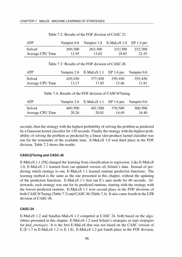
CHAPTER 7. MALES - MACHINE LEARNING OF STRATEGIES
Table 7.2: Results of the FOF division of CASC 23
ATP Vampire 0.6 Vampire 1.8 E-MaLeS 1.0 EP 1.4 pre
Solved 269/300 263/300 233/300 232/300Average CPU Time 12.95 13.62 18.85 22.55
Table 7.3: Results of the FOF division of CASC-J6
ATP Vampire 2.6 E-MaLeS 1.1 EP 1.6 pre Vampire 0.6
Solved 429/450 377/450 359/450 355/450Average CPU Time 13.17 17.85 13.46 11.81
Table 7.4: Results of the FOF division of CASC@Turing
ATP Vampire 2.6 E-MaLeS 1.1 EP 1.6 pre Vampire 0.6
Solved 469/500 401/500 378/500 368/500Average CPU Time 20.26 20.81 14.49 16.40
seconds, then the strategy with the highest probability of solving the problem as predictedby a Gaussian kernel classifier for 120 seconds. Finally the strategy with the highest prob-ability of solving the problem as predicted by a linear (dot-product) kernel classifier wasrun for the remainder of the available time. E-MaLeS 1.0 won third place in the FOFdivision. Table 7.2 shows the results.
CASC@Turing and CASC-J6
E-MaLeS 1.1 [58] changed the learning from classification to regression. Like E-MaLeS1.0, E-MaLeS 1.1 learned from (an updated version of) Schulz’s data. Instead of pre-dicting which strategy to run, E-MaLeS 1.1 learned runtime prediction functions. Thelearning method is the same as the one presented in this chapter, without the updatingof the prediction functions. E-MaLeS 1.1 first ran E’s auto mode for 60 seconds. Af-terwards, each strategy was run for its predicted runtime, starting with the strategy withthe lowest predicted runtime. E-MaLeS 1.1 won second place in the FOF divisions ofboth CASC@Turing (Table 7.3) and CASC-J6 (Table 7.4). It also came fourth in the LTBdivision of CASC-J6.
CASC-24
E-MaLeS 1.2 and Satallax-MaLeS 1.2 competed at CASC 24, both based on the algo-rithms presented in this chapter. E-MaLeS 1.2 used Schulz’s strategies as start strategiesfor find_strategies. It is the first E-MaLeS that was not based on the CASC version ofE (E 1.7 in E-MaLeS 1.2 vs E 1.8). E-MaLeS 1.2 got fourth place in the FOF division,
96
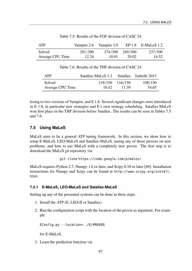
7.5. USING MALES
Table 7.5: Results of the FOF division of CASC 24
ATP Vampire 2.6 Vampire 3.0 EP 1.8 E-MaLeS 1.2
Solved 281/300 274/300 249/300 237/300Average CPU Time 12.24 10.91 29.02 14.52
Table 7.6: Results of the THF division of CASC 24
ATP Satallax-MaLeS 1.2 Satallax Isabelle 2013
Solved 119/150 116/150 108/150Average CPU Time 10.42 11.39 54.65
losing to two versions of Vampire, and E 1.8. Several significant changes were introducedin E 1.8, in particular new strategies and E’s own strategy scheduling. Satallax-MaLeSwon first place in the THF division before Satallax. The results can be seen in Tables 7.5and 7.6.
7.5 Using MaLeS
MaLeS aims to be a general ATP tuning framework. In this section, we show how tosetup E-MaLeS, LEO-MaLeS and Satallax-MaLeS, tuning any of those provers on newproblems, and how to use MaLeS with a completely new prover. The first step is todownload the MaLeS git repository via
git clone https://code.google.com/p/males/
MaLeS requires Python 2.7, Numpy 1.6 or later, and Scipy 0.10 or later [69]. Installationinstructions for Numpy and Scipy can be found at http://www.scipy.org/install.html.
7.5.1 E-MaLeS, LEO-MaLeS and Satallax-MaLeS
Setting up any of the presented systems can be done in three steps.
1. Install the ATP (E, LEO-II or Satallax)
2. Run the configuration script with the location of the prover as argument. For exam-ple
EConfig.py --location=../E/PROVER
for E-MaLeS.
3. Learn the prediction function via
97
CHAPTER 7. MALES - MACHINE LEARNING OF STRATEGIES
MaLeS/learn.py
After the installation, MaLeS can be used by running
MaLeS/males.py -t 30 -p test/PUZ001+1.p
where −t denotes the time limit and −p the problem to be solved.
7.5.2 Tuning E, LEO-II or Satallax for a New Set of Problems
Tuning an ATP for a particular dataset involves finding good search strategies and learningprediction models. The search behaviour is defined in the the file setup.ini in the maindirectory. Using the default search behaviour, E, LEO-II and Satallax can be tuned fornew data as follows:
1. Install the ATP (E, LEO-II or Satallax)
2. Run the configuration script with the location of the prover as argument. For exam-ple
EConfig.py --location=../E/PROVER
for E-MaLeS.
3. Store the absolute pathnames of the problems in a new file with one problem perline and change the PROBLEM parameter in setup.ini to the file containing theproblem paths.
4. Find promising strategies by searching with a short time limit (which is the defaultsetup)
MaLeS/findStrategies.py
5. Run all promising strategies for a longer time. For this several parameters need tobe changed.
a) Copy the value of ResultsDir to TmpResultsDir.
b) Copy the value of ResultsPickle to TmpResultsPickle.
c) Change the value of ResultsDir to a new directory.
d) Change the value of ResultsPickle to a new file.
e) Change Time in search to the maximal runtime (in seconds), e.g. 300.
f) Set FullTime to True.
g) Set TryWithNewDefaultTime to True.
6. Run findStrategies again.
98
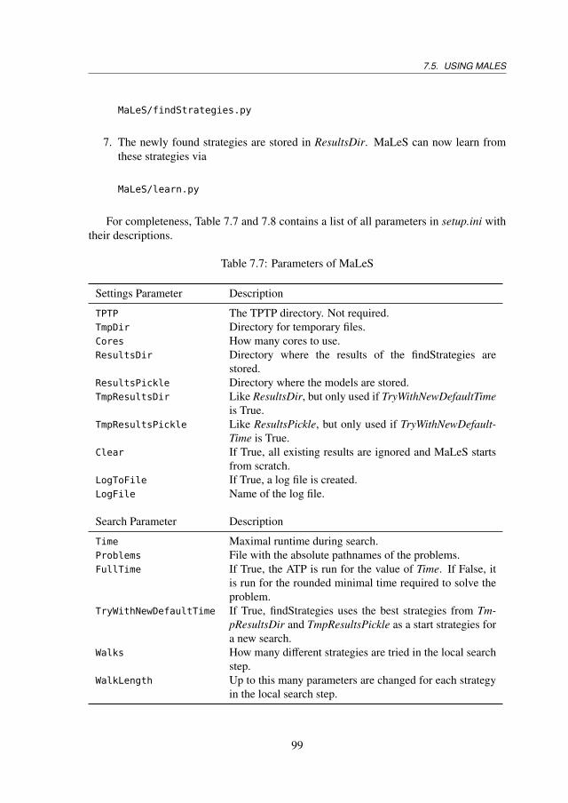
7.5. USING MALES
MaLeS/findStrategies.py
7. The newly found strategies are stored in ResultsDir. MaLeS can now learn fromthese strategies via
MaLeS/learn.py
For completeness, Table 7.7 and 7.8 contains a list of all parameters in setup.ini withtheir descriptions.
Table 7.7: Parameters of MaLeS
Settings Parameter Description
TPTP The TPTP directory. Not required.TmpDir Directory for temporary files.Cores How many cores to use.ResultsDir Directory where the results of the findStrategies are
stored.ResultsPickle Directory where the models are stored.TmpResultsDir Like ResultsDir, but only used if TryWithNewDefaultTime
is True.TmpResultsPickle Like ResultsPickle, but only used if TryWithNewDefault-
Time is True.Clear If True, all existing results are ignored and MaLeS starts
from scratch.LogToFile If True, a log file is created.LogFile Name of the log file.
Search Parameter Description
Time Maximal runtime during search.Problems File with the absolute pathnames of the problems.FullTime If True, the ATP is run for the value of Time. If False, it
is run for the rounded minimal time required to solve theproblem.
TryWithNewDefaultTime If True, findStrategies uses the best strategies from Tm-pResultsDir and TmpResultsPickle as a start strategies fora new search.
Walks How many different strategies are tried in the local searchstep.
WalkLength Up to this many parameters are changed for each strategyin the local search step.
99

CHAPTER 7. MALES - MACHINE LEARNING OF STRATEGIES
Table 7.8: Parameters of MaLeS (cont.)
Learn Parameter Description
Features Which features to use. Possible values are E for the Efeatures and TPTP for the TPTP features.
FeaturesFile Location of the feature file.StrategiesFile Location of the strategies file.KernelFile Location of the file containing the kernel matrices.RegularizationGrid Possible values for λ.KernelGrid Possible values for σ.CrossValidate If False, no crossvalidation is done during learning. In-
stead the first values in RegularizationGrid and Kernel-Grid are used.
CrossValidationFolds How many folds to use during crossvalidation.StartStrategies Number of start strategies.StartStrategiesTime Runtime of each start strategy.CPU Bias This value is added to each runtime before learning.
Serves as a buffer against runtime irregularities.Tolerance For a strategy s to be considered as a good strategy, there
must be at least one problem where the difference of thebest runtime of any strategy and the runtime of s is at mostthis value.
Run Parameter Description
CPUSpeedRatio Predicted runtimes are multiplied with this value. Usefulif the training was done on a different machine.
MinRunTime Minimal time a strategy is run.Features Either TPTP for higher order features or E for first order
features.StrategiesFile Location of the strategies file.FeaturesFile Location of the feature file.OutputFile If not None, the output of MaLeS is stored in this file.
100
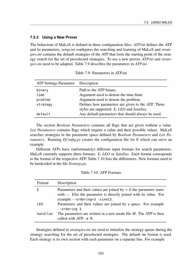
7.5. USING MALES
7.5.3 Using a New Prover
The behaviour of MaLeS is defined in three configuration files: ATP.ini defines the ATPand its parameters, setup.ini configures the searching and learning of MaLeS and strate-gies.ini contains the default strategies of the ATP that form the starting point of the strat-egy search for the set of preselected strategies. To use a new prover, ATP.ini and strate-gies.ini need to be adapted. Table 7.9 describes the parameters in ATP.ini.
Table 7.9: Parameters in ATP.ini
ATP Settings Parameter Description
binary Path to the ATP binary.time Argument used to denote the time limit.problem Argument used to denote the problem.strategy Defines how parameters are given to the ATP. Three
styles are supported: E, LEO and Satallax.default Any default parameters that should always be used.
The section Boolean Parameters contains all flags that are given without a value.List Parameters contains flags which require a value and their possible values. MaLeSsearches strategies in the parameter space defined by Boolean Parameters and List Pa-rameters. Running EConfig.py creates the configuration file for E which can serve anexample.
Different ATPs have (unfortunately) different input formats for search parameters.MaLeS currently supports three formats: E, LEO or Satallax. Each format correspondsto the format of the respective ATP. Table 7.10 lists the differences. New formats need tobe hardcoded in the file Strategy.py.
Table 7.10: ATP Formats
Format Description
E Parameters and their values are joined by = if the parameter startswith --. Else the parameter is directly joined with its value. Forexample --ordering=3 -sine13.
LEO Parameters and their values are joined by a space. For example--ordering 3.
Satallax The parameters are written in a new mode file M. The ATP is thencalled with ATP -m M.
Strategies defined in strategies.ini are used to initialize the strategy queue during thestrategy searching for the set of preselected strategies. The default ini format is used.Each strategy is its own section with each parameter on a separate line. For example
101
CHAPTER 7. MALES - MACHINE LEARNING OF STRATEGIES
[NewStrategy12884]
FILTER_START = 0
ENUM_IMP = 100
INITIAL_SUBTERMS_AS_INSTANTIATIONS = true
E_TIMEOUT = 1
POST_CONFRONT3_DELAY = 1000
FORALL_DELAY = 0
LEIBEQ_TO_PRIMEQ = true
At least one strategy must be defined. After the ini files are adapted, the new ATP canbe tuned and run using the procedure defined in the last two sections.
7.6 Future Work
Apart from simplifying the installation and set up, there are several other ways to improveMaLeS. We present the three most promising ones.
Features: The quality of the runtime prediction function is limited by the quality of thefeatures. Adding new features and using feature selection methods could increase theprediction capabilities of MaLeS.
Strategy Finding: As an alternative to randomized hill climbing, different search algo-rithms should be supported. In particular simulated annealing and genetic algorithmsseem promising. The biggest problem of the current implementation, the time it needsto find good strategies, could be improved by using a clusterized local search principlesimilar to the one employed in BliStr [107].
Strategy Prediction: The runtime prediction function are the heart of MaLeS. Machinelearning offers dozens of different regression methods which could be used instead of thekernel methods of MaLeS. A big drawback of the current method is that it scales badlydue to the need to invert a new matrix after every tried strategy. A nearest neighbourapproach would eliminate the need for matrix computations and also the dependency onNumpy and Scipy.
7.7 Conclusion
Finding the best parameter settings and strategy schedules for an ATP is a time consum-ing task that often requires in-depth knowledge of how the ATP works. MaLeS is anautomatic tuning framework for ATPs. Given the possible parameter settings of an ATPand a set of problems, MaLeS finds good search strategies and creates individual strategyschedules. MaLeS currently supports E, LEO-II and Satallax and can easily be extendedto work with other provers.
Experiments with the ATPs E, LEO-II and Satallax showed that the MaLeS versionperforms at least comparable to the respective default strategy selection algorithm. In
102
7.7. CONCLUSION
some cases, the MaLeS optimized version solves considerably more problems than theuntuned ATP.
MaLeS simplifies the workflow for both ATP users and developers. It allows ATPusers to fine-tune ATPs to their specific problems and helps ATP developers to focus onactual improvements instead of time-consuming parameter tuning.
103

Contributions
The detailed contributions to each chapter are listed here. Josef Urban proof read thecomplete thesis and suggested many improvements.
Chapter 1 and Chapter 2 are, apart from Section 1.3 and 2.2, based on joint work withJasmin Blanchette. The paper is titled “A Survey of Axiom Selection as a Machine Learn-ing Problem” and submitted to “Infinity, computability, and metamathematics. Festschriftcelebrating the 60th birthdays of Peter Koepke and Philip Welch”. I did most of the writ-ing and all evaluations, Jasmin provided the raw Isabelle data upon which the figures andtables are based.
Section 2.2 is based on [2] “Premise Selection for Mathematics by Corpus Analysisand Kernel Methods”, published in the Journal of Automated Reasoning. Section 2.2.1 ismostly written by Josef Urban. Section 2.2.2 was written by me and proof read by TomHeskes. Section 2.2.3 was originally written by Evgeni Tsivtsivadze, the current versionwas mainly written by myself with input from all other co-authors. Evgeni had the ideafor Section 2.2.4. The implementation was done by myself (based on earlier code by Ev-geni). The text of the section was written by myself, Evgeni, and Tom.
Chapter 3 is based on [57] “Overview and Evaluation of Premise Selection Techniquesfor Large Theory Mathematics”, published in the Proceedings of the 6th InternationalJoint Conference on Automated Reasoning. The introduction is based on an earlier work-shop paper by Josef Urban [106]. SNoW had already been used in earlier work by Josef[102, 105]. MOR-CG was developed by me with help from Evgeni Tsivtsivadze. Twanvan Laarhoven created BiLi. Section 3.2 is my work. The data for Section 3.3 was createdby me and Josef. I wrote the text, Josef proof read. Section 3.4 was done by Josef. TomHeskes, Evgeni and Twan helped with polishing the paper.
Chapter 4 is based on: [55] “Learning from Multiple Proofs: First Experiments”, pub-lished in the Proceedings of the 3rd Workshop on Practical Aspects of Automated Rea-soning. I did the writing and the machine learning experiments. Josef Urban did the ATPevaluations and proof read the paper.
105
CONTRIBUTIONS
Chapter 5 is based on: [3] “Automated and Human Proofs in General Mathematics: AnInitial Comparison”, published in the Proceedings of the 18th International Conferenceon Logic for Programming, Artificial Intelligence, and Reasoning. All three authors con-tributed equally to the paper. The proof dependencies in Section 5.2.1 were created byJesse Alama and Josef Urban. The final version of the text of 5.2.1 was written by Josefas a part of our joint work on paper [2] “Premise Selection for Mathematics by CorpusAnalysis and Kernel Methods”, published in the Journal of Automated Reasoning.
Chapter 6 is based on: [56] “MaSh: Machine Learning for Sledgehammer”, publishedin the Proceedings of the 4th International Conference on Interactive Theorem Proving.Jasmin Blanchette developed the Isabelle side of MaSh. I programmed the Python partof MaSh and was responsible for the machine learning evaluation. Cezary Kaliszyk andJasmin did the ATP evaluation. Josef Urban did some proof reading and acted as generaladvisor.
Chapter 7 is based on: [53] “MaLeS: A Framework for Automatic Tuning of AutomatedTheorem Provers” , currently under review at the Journal for Automated Reasoning; andan extension of joint work with Stephan Schulz and Josef Urban [58] “E-MaLeS 1.1”,published in the Proceedings of the 24th Conference on Automated Deduction. I wrotethis paper, implemented the MaLeS system, and did all the experiments. Josef Urbanadvised me. Both Stephan Schulz and Josef helped with proof reading the paper. Thewriting of the earlier E-MaLeS 1.1 paper was done equally by me and Josef, Stephancontributed some E-related parts and suggested improvements.
106
Bibliography
[1] The Mizar Mathematical Library. http://mizar.org/.
[2] Jesse Alama, Tom Heskes, Daniel Kühlwein, Evgeni Tsivtsivadze, and Josef Ur-
ban. Premise Selection for Mathematics by Corpus Analysis and Kernel Methods.
Journal of Automated Reasoning, pages 1–23, 2013. doi:10.1007/s10817-013-
9286-5.
[3] Jesse Alama, Daniel Kühlwein, and Josef Urban. Automated and Human Proofs
in General Mathematics: An Initial Comparison. In Nikolaj Bjørner and Andrei
Voronkov, editors, Logic for Programming, Artificial Intelligence, and Reasoning,
volume 7180 of Lecture Notes in Computer Science, pages 37–45. Springer, 2012.
doi:10.1007/978-3-642-28717-6_6.
[4] Jesse Alama, Lionel Mamane, and Josef Urban. Dependencies in Formal Mathe-
matics: Applications and Extraction for Coq and Mizar. In Johan Jeuring, JohnA.
Campbell, Jacques Carette, Gabriel Reis, Petr Sojka, Makarius Wenzel, and Volker
Sorge, editors, Intelligent Computer Mathematics, volume 7362 of Lecture Notes
in Computer Science, pages 1–16. Springer, 2012. doi:10.1007/978-3-642-
31374-5_1.
[5] N. Aronszajn. Theory of reproducing kernels. Transactions of the American Math-
ematical Society, 68, 1950. doi:10.1090/S0002-9947-1950-0051437-7.
[6] Jeremy Avigad, Kevin Donnelly, David Gray, and Paul Raff. A formally verified
proof of the prime number theorem. ACM Transactions on Computational Logic
(TOCL), 9(1):2, 2007. doi:10.1145/1297658.1297660.
107
BIBLIOGRAPHY
[7] Thomas Ball, Ella Bounimova, Vladimir Levin, Rahul Kumar, and Jakob Lichten-
berg. The Static Driver Verifier Research Platform. In Tayssir Touili, Byron Cook,
and Paul Jackson, editors, Computer Aided Verification, volume 6174 of Lecture
Notes in Computer Science, pages 119–122. Springer, 2010. doi:10.1007/978-
3-642-14295-6_11.
[8] Clark Barrett and Cesare Tinelli. CVC3. In Werner Damm and Holger Hermanns,
editors, Computer Aided Verification, volume 4590 of Lecture Notes in Computer
Science, pages 298–302. Springer, 2007. doi:10.1007/978-3-540-73368-3_34.
[9] Christoph Benzmüller, Lawrence C. Paulson, Frank Theiss, and Arnaud Fietzke.
LEO-II - A Cooperative Automatic Theorem Prover for Classical Higher-Order
Logic (System Description). In Alessandro Armando, Peter Baumgartner, and
Gilles Dowek, editors, Automated Reasoning, volume 5195 of Lecture Notes in
Computer Science, pages 162–170. Springer, 2008. doi:10.1007/978-3-540-
71070-7_14.
[10] Stefan Berghofer and Tobias Nipkow. Proof Terms for Simply Typed Higher Order
Logic. In Mark Aagaard and John Harrison, editors, Theorem Proving in Higher
Order Logics, volume 1869 of Lecture Notes in Computer Science, pages 38–52.
Springer, 2000. doi:10.1007/3-540-44659-1_3.
[11] Yves Bertot and Pierre Castéran. Interactive Theorem Proving and Program
Development—Coq’Art: The Calculus of Inductive Constructions. Texts in Theo-
retical Computer Science. Springer, 2004.
[12] Ella Bingham and Heikki Mannila. Random Projection in Dimensionality Reduc-
tion: Applications to Image and Text Data. In Proceedings of the Seventh Inter-
national Conference on Knowledge Discovery and Data Mining, pages 245–250.
ACM Press, 2001. doi:10.1145/502512.502546.
[13] Christopher M. Bishop. Pattern Recognition and Machine Learning. Information
Science and Statistics. Springer, 2006.
[14] Jasmin Christian Blanchette, Sascha Böhme, Andrei Popescu, and Nicholas Small-
bone. Encoding Monomorphic and Polymorphic Types. In Nir Piterman and Scott
Smolka, editors, Proceedings of the 19th international conference on Tools and
108
BIBLIOGRAPHY
Algorithms for the Construction and Analysis of Systems, volume 7795 of Lecture
Notes in Computer Science. Springer, 2013. doi:10.1007/978-3-642-36742-
7_34.
[15] Jasmin Christian Blanchette, Lukas Bulwahn, and Tobias Nipkow. Automatic
Proof and Disproof in Isabelle/HOL. In Cesare Tinelli and Viorica Sofronie-
Stokkermans, editors, Proceedings of the 8th international conference on Frontiers
of combining systems, volume 6989 of Lecture Notes in Computer Science, pages
12–27. Springer, 2011. doi:10.1007/978-3-642-24364-6_2.
[16] Jasmin Christian Blanchette, Sascha Böhme, and Lawrence C. Paulson. Extending
Sledgehammer with SMT solvers. Journal of Automated Reasoning, 51(1):109–
128, 2013. doi:10.1007/s10817-013-9278-5.
[17] Jasmin Christian Blanchette, Andrei Popescu, Daniel Wand, and Christoph Wei-
denbach. More SPASS with Isabelle. In Lennart Beringer and Amy Felty, editors,
Interactive Theorem Proving, volume 7406 of Lecture Notes in Computer Science,
pages 345–360. Springer, 2012. doi:10.1007/978-3-642-32347-8_24.
[18] James P. Bridge. Machine learning and automated theorem proving. University of
Cambridge, Computer Laboratory, Technical Report, (792), 2010.
[19] Chad E. Brown. Satallax: An Automatic Higher-Order Prover. In Bernhard
Gramlich, Dale Miller, and Uli Sattler, editors, Automated Reasoning, volume
7364 of Lecture Notes in Computer Science, pages 111–117. Springer, 2012.
doi:10.1007/978-3-642-31365-3_11.
[20] Sascha Böhme and Tobias Nipkow. Sledgehammer: Judgement Day. In Jürgen
Giesl and Reiner Hähnle, editors, Automated Reasoning, volume 6173 of Lecture
Notes in Computer Science, pages 107–121. Springer, 2010. doi:10.1007/978-
3-642-14203-1_9.
[21] Andy Carlson, Chad Cumby, Jeff Rosen, and Dan Roth. The SNoW Learning
Architecture. Technical Report UIUCDCS-R-99-2101, UIUC Computer Science
Department, May 1999.
[22] Gregory J. Chaitin. The Omega Number: Irreducible Complexity in Pure Math.
In Jonathan M. Borwein and William M. Farmer, editors, Proceedings of the 5th
109
BIBLIOGRAPHY
International Conference on Mathematical Knowledge Management, volume 4108
of Lecture Notes in Computer Science, page 1. Springer, 2006. doi:10.1007/
11812289_1.
[23] Wei Chu and Seung-Taek Park. Personalized Recommendation on Dynamic
Content Using Predictive Bilinear Models. In Proceedings of the 18th Inter-
national Conference on World Wide Web, pages 691–700. ACM Press, 2009.
doi:10.1145/1526709.1526802.
[24] Marcos Cramer, Peter Koepke, Daniel Kühlwein, and Bernhard Schröder. Premise
Selection in the Naproche System. In Jürgen Giesl and Reiner Hähnle, editors,
Automated Reasoning, volume 6173 of Lecture Notes in Computer Science, pages
434–440. Springer, 2010. doi:10.1007/978-3-642-14203-1_37.
[25] Ingo Dahn. Robbins Algebras Are Boolean: A Revision of McCune’s Computer-
Generated Solution of Robbins Problem. Journal of Algebra, 208:526–532, 1998.
doi:10.1006/jabr.1998.7467.
[26] Scott Deerwester, Susan T. Dumais, George W. Furnas, Thomas K. Landauer, and
Richard Harshman. Indexing by latent semantic analysis. Journal of the Ameri-
can Society for Information Science, 41(6):391–407, 1990. doi:10.1002/(SICI)
1097-4571(199009)41:6<391::AID-ASI1>3.0.CO;2-9.
[27] Kosta Dosen. Identity of proofs based on normalization and generality. Bulletin of
Symbolic Logic, 9:477–503, 2003.
[28] Bruno Dutertre and Leonardo de Moura. The Yices SMT solver. http://yices.
csl.sri.com/tool-paper.pdf, 2006.
[29] Branden Fitelson. Using Mathematica to understand the computer proof of the
Robbins Conjecture. Mathematica In Education and Research, 7(1), 1998.
[30] Gottlob Frege. Begriffsschrift, eine der arithmetischen nachgebildete Formel-
sprache des reinen Denkens. Verlag von Louis Nebert, Halle, 1879.
[31] Matthias Fuchs. Automatic Selection Of Search-Guiding Heuristics For Theorem
Proving. In Proceedings of the 10th Florida AI Research Society Conference, pages
1–5. Florida AI Research Society, 1998.
110
BIBLIOGRAPHY
[32] Kurt Gödel. Über formal unentscheidbare Sätze der Principia Mathematica und
verwandter Systeme I. Monatshefte für Mathematik und Physik, 38(1):173–198,
1931.
[33] Georges Gonthier. Formal Proof—The Four-Color Theorem. Notices of the AMS,
55(11):1382–1393, 2008.
[34] Georges Gonthier, Andrea Asperti, Jeremy Avigad, Yves Bertot, Cyril Co-
hen, François Garillot, Stéphane Le Roux, Assia Mahboubi, Russell O’Connor,
Sidi Ould Biha, Ioana Pasca, Laurence Rideau, Alexey Solovyev, Enrico Tassi,
and Laurent Théry. A Machine-Checked Proof of the Odd Order Theorem. In
Sandrine Blazy, Christine Paulin-Mohring, and David Pichardie, editors, Interac-
tive Theorem Proving, volume 7998 of Lecture Notes in Computer Science, pages
163–179. Springer, 2013. doi:10.1007/978-3-642-39634-2_14.
[35] Adam Grabowski, Artur Korniłowicz, and Adam Naumowicz. Mizar in a Nut-
shell. Journal of Formalized Reasoning, 3(2):153–245, 2010. doi:10.6092/issn.
1972-5787/1980.
[36] Isabelle Guyon and André Elisseeff. An introduction to variable and feature selec-
tion. Journal of Machine Learning Research, 3:1157–1182, March 2003.
[37] Thomas C. Hales. Introduction to the Flyspeck project. In Thierry Coquand, Henri
Lombardi, and Marie-Françoise Roy, editors, Mathematics, Algorithms, Proofs,
volume 05021 of Dagstuhl Seminar Proceedings. Internationales Begegnungs- und
Forschungszentrum für Informatik (IBFI), Schloss Dagstuhl, Germany, 2005.
[38] Thomas C. Hales. Mathematics in the age of the Turing machine. Lecture Notes in
Logic, 2012. to appear; http://www.math.pitt.edu/~thales/papers/turing.
pdf.
[39] John Harrison. HOL Light: A tutorial introduction. In Mandayam Srivas and
Albert Camilleri, editors, Formal Methods in Computer-Aided Design, volume
1166 of Lecture Notes in Computer Science, pages 265–269. Springer, 1996.
doi:10.1007/BFb0031814.
[40] John Harrison. Formal verification of IA-64 division algorithms. In Mark Aagaard
and John Harrison, editors, Theorem Proving in Higher Order Logics, volume 1869
111
BIBLIOGRAPHY
of Lecture Notes in Computer Science, pages 233–251. Springer, 2000. doi:10.
1007/3-540-44659-1_15.
[41] Kryštof Hoder and Andrei Voronkov. Sine Qua Non for Large Theory Reason-
ing. In Nikolaj Bjørner and Viorica Sofronie-Stokkermans, editors, Automated
Deduction, volume 6803 of Lecture Notes in Computer Science, pages 299–314.
Springer, 2011. doi:10.1007/978-3-642-22438-6_23.
[42] Johannes Hölzl and Armin Heller. Three chapters of measure theory in Is-
abelle/HOL. In Marko C. J. D. van Eekelen, Herman Geuvers, Julien Schmaltz,
and Freek Wiedijk, editors, Proceedings of the 2nd Conference on Interactive The-
orem Proving, volume 6898 of Lecture Notes in Computer Science, pages 135–151.
Springer, 2011. doi:10.1007/978-3-642-22863-6_12.
[43] Joe Hurd. First-order proof tactics in higher-order logic theorem provers. In Myla
Archer, Ben Di Vito, and César Muñoz, editors, Design and Application of Strate-
gies/Tactics in Higher Order Logics, number CP-2003-212448 in NASA Tech. Re-
ports, pages 56–68, 2003.
[44] Frank Hutter, Holger H. Hoos, Kevin Leyton-Brown, and Thomas Stützle.
ParamILS: An Automatic Algorithm Configuration Framework. Journal of Artifi-
cial Intelligence Research, 36:267–306, October 2009. doi:10.1613/jair.2861.
[45] Cezary Kaliszyk and Josef Urban. Learning-assisted Automated Reasoning with
Flyspeck. CoRR, abs/1211.7012, 2012. http://arxiv.org/abs/1211.7012.
[46] Cezary Kaliszyk and Josef Urban. Automated Reasoning Service for HOL Light.
In Jacques Carette, David Aspinall, Christoph Lange, Petr Sojka, and Wolfgang
Windsteiger, editors, Intelligent Computer Mathematics, volume 7961 of Lecture
Notes in Computer Science, pages 120–135. Springer, 2013. doi:10.1007/978-
3-642-39320-4_8.
[47] Matt Kaufmann, Panagiotis Manolios, and J Strother Moore. Computer-Aided
Reasoning: An Approach. Kluwer Academic Publishers, 2000.
[48] Gerwin Klein, June Andronick, Kevin Elphinstone, Gernot Heiser, David Cock,
Philip Derrin, Dhammika Elkaduwe, Kai Engelhardt, Rafal Kolanski, Michael
112
BIBLIOGRAPHY
Norrish, Thomas Sewell, Harvey Tuch, and Simon Winwood. seL4: formal veri-
fication of an operating-system kernel. Communications of the ACM, 53(6):107–
115, 2010. doi:10.1145/1743546.1743574.
[49] Gerwin Klein and Tobias Nipkow. Jinja is not Java. In Gerwin Klein, Tobias
Nipkow, and Lawrence Paulson, editors, Archive of Formal Proofs. http://afp.
sf.net/entries/Jinja.shtml, 2005.
[50] Gerwin Klein, Tobias Nipkow, and Lawrence Paulson, editors. Archive of Formal
Proofs. http://afp.sf.net/.
[51] Ron Kohavi. A study of cross-validation and bootstrap for accuracy estimation
and model selection. In Proceedings of the 14th international joint conference on
Artificial intelligence - Volume 2, pages 1137–1143. Morgan Kaufmann Publishers
Inc., 1995.
[52] Steven G Krantz. The history and concept of mathematical proof. 2007.
[53] D. Kühlwein and J. Urban. MaLeS: A Framework for Automatic Tuning of Auto-
mated Theorem Provers. ArXiv e-prints, August 2013. arXiv:1308.2116.
[54] Daniel Kühlwein, Stephan Schulz, and Josef Urban. Experiments with Strategy
Learning for E Prover. In 2nd Joint International Workshop on Strategies in
Rewriting, Proving and Programming. 2012.
[55] Daniel Kühlwein and Josef Urban. Learning from multiple proofs: First experi-
ments. In Pascal Fontaine, Renate A. Schmidt, and Stephan Schulz, editors, Prac-
tical Aspects of Automated Reasoning, volume 21 of EPiC Series, pages 82–94.
EasyChair, 2013.
[56] Daniel Kühlwein, Jasmin Christian Blanchette, Cezary Kaliszyk, and Josef Urban.
MaSh: Machine Learning for Sledgehammer. In Sandrine Blazy, Christine Paulin-
Mohring, and David Pichardie, editors, Interactive Theorem Proving, volume 7998
of Lecture Notes in Computer Science, pages 35–50. Springer, 2013. doi:10.
1007/978-3-642-39634-2_6.
[57] Daniel Kühlwein, Twan Laarhoven, Evgeni Tsivtsivadze, Josef Urban, and Tom
Heskes. Overview and Evaluation of Premise Selection Techniques for Large The-
ory Mathematics. In Bernhard Gramlich, Dale Miller, and Uli Sattler, editors,
113
BIBLIOGRAPHY
Automated Reasoning, volume 7364 of Lecture Notes in Computer Science, pages
378–392. Springer, 2012. doi:10.1007/978-3-642-31365-3_30.
[58] Daniel Kühlwein, Stephan Schulz, and Josef Urban. E-MaLeS 1.1. In Maria Paola
Bonacina, editor, Automated Deduction – CADE-24, volume 7898 of Lecture Notes
in Computer Science, pages 407–413. Springer, 2013. doi:10.1007/978-3-642-
38574-2_28.
[59] Huan Liu and Hiroshi Motoda. Feature Selection for Knowledge Discovery and
Data Mining. Kluwer Academic Publishers, 1998. doi:10.1007/978-1-4615-
5689-3.
[60] David J.C. MacKay. Information Theory, Inference and Learning Algorithms.
Cambridge University Press, 2003. doi:10.2277/0521642981.
[61] Roman Matuszewski and Piotr Rudnicki. Mizar: The first 30 years. Mechanized
Mathematics and Its Applications, 4:3–24, 2005.
[62] William Mccune. Solution of the Robbins problem. Journal of Automated Rea-
soning, 19(3):263–276, 1997. doi:10.1023/A:1005843212881.
[63] William McCune. Prover9 and Mace4. http://www.cs.unm.edu/~mccune/
prover9/, 2005–2010.
[64] Jia Meng and Lawrence C. Paulson. Lightweight relevance filtering for machine-
generated resolution problems. Journal of Applied Logic, 7(1):41–57, 2009. doi:
10.1016/j.jal.2007.07.004.
[65] J. Strother Moore, Thomas W. Lynch, and Matt Kaufmann. A mechanically
checked proof of the AMD5K86TM floating point division program. IEEE Transac-
tions on Computers, 47(9):913–926, 1998. doi:10.1109/12.713311.
[66] Leonardo Moura and Nikolaj Bjørner. Z3: An Efficient SMT Solver. In C.R.
Ramakrishnan and Jakob Rehof, editors, Tools and Algorithms for the Construc-
tion and Analysis of Systems, volume 4963 of Lecture Notes in Computer Science,
pages 337–340. Springer, 2008. doi:10.1007/978-3-540-78800-3_24.
[67] Kevin P. Murphy. Machine Learning: A Probabilistic Perspective. MIT Press,
2012.
114
BIBLIOGRAPHY
[68] Tobias Nipkow, Lawrence C. Paulson, and Markus Wenzel. Isabelle/HOL: A Proof
Assistant for Higher-Order Logic, volume 2283 of Lecture Notes in Computer Sci-
ence. Springer, 2002.
[69] Travis E. Oliphant. Python for scientific computing. Computing in Science &
Engineering, 9(3):10–20, 2007. doi:10.1109/MCSE.2007.58.
[70] Jens Otten and Wolfgang Bibel. leanCoP: lean connection-based theorem proving.
Journal of Symbolic Computation, 36(1–2):139 – 161, 2003. doi:http://dx.
doi.org/10.1016/S0747-7171(03)00037-3.
[71] Sam Owre and Natarajan Shankar. A brief overview of PVS. In Theorem Proving
in Higher Order Logics, volume 5170 of Lecture Notes in Computer Science, pages
22–27. Springer, 2008. doi:10.1007/978-3-540-71067-7_5.
[72] Lawrence C. Paulson. The inductive approach to verifying cryptographic proto-
cols. Journal of Computer Security, 6(1-2):85–128, 1998.
[73] Lawrence C. Paulson and Jasmin Christian Blanchette. Three years of experience
with Sledgehammer, a Practical Link Between Automatic and Interactive Theorem
Provers. In Geoff Sutcliffe, Stephan Schulz, and Eugenia Ternovska, editors, In-
ternational Workshop on the Implementation of Logics 2010, volume 2 of EPiC
Series, pages 1–11. EasyChair, 2012.
[74] J.D. Phillips and D. Stanovský. Automated Theorem Proving in Loop Theory.
In G. Sutcliffe, S. Colton, and S. Schulz, editors, Proceedings of the Workshop
on Empirically Successful Automated Reasoning for Mathematics, number 378 in
CEUR Workshop Proceedings, pages 42–53, 2008.
[75] Robi Polikar. Ensemble based systems in decision making. Circuits and Systems
Magazine, IEEE, 6(3):21–45, 2006. doi:10.1109/MCAS.2006.1688199.
[76] Petr Pudlak. Semantic Selection of Premisses for Automated Theorem Proving.
In Geoff Sutcliffe, Josef Urban, and Stephan Schulz, editors, Proceedings of the
CADE-21 Workshop on Empirically Successful Automated Reasoning in Large
Theories, volume 257 of CEUR Workshop Proceedings, 2007.
[77] Alexandre Riazanov and Andrei Voronkov. The design and implementation of
VAMPIRE. AI Communications, 15(2-3):91–110, August 2002.
115
BIBLIOGRAPHY
[78] Ryan Rifkin, Gene Yeo, and Tomaso Poggio. Regularized least-squares classifi-
cation. In J.A.K. Suykens, G. Horvath, S. Basu, C. Micchelli, and J. Vandewalle,
editors, Advances in Learning Theory: Methods, Model and Applications, pages
131–154, Amsterdam, 2003. IOS Press.
[79] Alex Roederer, Yury Puzis, and Geoff Sutcliffe. Divvy: An ATP Meta-system
Based on Axiom Relevance Ordering. In Schmidt [80], pages 157–162. doi:
10.1007/978-3-642-02959-2.
[80] Renate A. Schmidt, editor. Automated Deduction, volume 5663 of Lecture Notes
in Computer Science. Springer, 2009. doi:10.1007/978-3-642-02959-2.
[81] Bernhard Schoelkopf, Ralf Herbrich, Robert Williamson, and Alex J Smola. A
Generalized Representer Theorem. In D. Helmbold and R. Williamson, editors,
Proceedings of the 14th Annual Conference on Computational Learning Theory,
pages 416–426, 2001. doi:10.1007/3-540-44581-1_27.
[82] Bernhard Scholkopf and Alexander J. Smola. Learning with Kernels: Support Vec-
tor Machines, Regularization, Optimization, and Beyond. MIT Press, Cambridge,
MA, USA, 2001.
[83] Stephan Schulz. Learning search control knowledge for equational deduction,
volume 230 of Dissertations in Artificial Intelligence. Infix Akademische Verlags-
gesellschaft, 2000.
[84] Stephan Schulz. E—A Brainiac Theorem Prover. Journal of AI Communications,
15(2-3):111–126, 2002.
[85] Stephan Schulz. System description: E 0.81. In David Basin and Michaël Rusi-
nowitch, editors, Automated Reasoning, volume 3097 of Lecture Notes in Com-
puter Science, pages 223–228. Springer, 2004. doi:10.1007/978-3-540-25984-
8_15.
[86] Stephan Schulz. First-order deduction for large knowledge bases. Presentation at
Deduction at Scale Seminar, 2011.
[87] D. Sculley. Rank aggregation for similar items. In Proceedings of 2007 SIAM In-
ternational Conference on Data Mining. Society for Industrial and Applied Math-
ematics, 2007.
116
BIBLIOGRAPHY
[88] John Shawe-Taylor and Nello Cristianini. Kernel Methods for Pattern Analysis.
Cambridge University Press, 2004.
[89] Jonathan R Shewchuk. An Introduction to the Conjugate Gradient Method Without
the Agonizing Pain. Technical report, 1994.
[90] Konrad Slind and Michael Norrish. A Brief Overview of HOL4. In Otmane Ait
Mohamed, César Muñoz, and Sofiène Tahar, editors, Theorem Proving in Higher
Order Logics, volume 5170 of Lecture Notes in Computer Science, pages 28–32.
Springer, 2008. doi:10.1007/978-3-540-71067-7_6.
[91] Geoff Sutcliffe. The TPTP problem library and associated infrastructure. Journal of
Automated Reasoning, 43(4):337–362, 2009. doi:10.1007/s10817-009-9143-8.
[92] Geoff Sutcliffe. The CADE-22 Automated Theorem Proving System Competition
- CASC-22. AI Communications, 23(1):47–60, 2010.
[93] Geoff Sutcliffe. The 5th IJCAR Automated Theorem Proving System Competition
- CASC-J5. AI Communications, 24(1):75–89, 2011.
[94] Geoff Sutcliffe. The CADE-23 Automated Theorem Proving System Competition
- CASC-23. AI Communications, 25(1):49–63, 2012.
[95] Geoff Sutcliffe. The 6th IJCAR automated theorem proving system competition—
CASC-J6. AI Communications, 26(2):211–223, 2013.
[96] Geoff Sutcliffe and Christoph Benzmüller. Automated reasoning in higher-order
logic using the TPTP THF infrastructure. Journal of Formalized Reasoning,
3(1):1–27, 2010.
[97] Geoff Sutcliffe and Yury Puzis. SRASS - A Semantic Relevance Axiom Selec-
tion System. In Frank Pfenning, editor, Proceedings of the 21st Conference on
Automated Deduction, volume 4603 of Lecture Notes in Computer Science, pages
295–310. Springer, 2007. doi:10.1007/978-3-540-73595-3_20.
[98] Geoff Sutcliffe and Christian Suttner. Evaluating General Purpose Automated
Theorem Proving Systems. Artificial Intelligence, 131(1-2):39–54, 2001. doi:
10.1016/S0004-3702(01)00113-8.
117
BIBLIOGRAPHY
[99] Tanel Tammet. Gandalf. Journal of Automated Reasoning, 18:199–204, 1997.
doi:10.1023/A:1005887414560.
[100] Evgeni Tsivtsivadze, Tapio Pahikkala, Jorma Boberg, Tapio Salakoski, and Tom
Heskes. Co-Regularized Least-Squares for Label Ranking. In Johannes Fürnkranz
and Eyke Hüllermeier, editors, Preference Learning, pages 107–123. Springer,
2011. doi:10.1007/978-3-642-14125-6_6.
[101] Josef Urban. MPTP – Motivation, Implementation, First Experiments. Journal
of Automated Reasoning, 33(3-4):319–339, 2004. doi:10.1007/s10817-004-
6245-1.
[102] Josef Urban. MizarMode—an integrated proof assistance tool for the Mizar way
of formalizing mathematics. Journal of Applied Logic, 4(4):414–427, 2006. doi:
10.1016/j.jal.2005.10.004.
[103] Josef Urban. MoMM - fast interreduction and retrieval in large libraries of
formalized mathematics. International Journal on Artificial Intelligence Tools,
15(1):109–130, 2006. doi:10.1142/S0218213006002588.
[104] Josef Urban. MPTP 0.2: Design, Implementation, and Initial Experiments. Journal
of Automated Reasoning, 37(1-2):21–43, 2006. doi:10.1007/s10817-006-9032-
3.
[105] Josef Urban. MaLARea: A metasystem for automated reasoning in large theo-
ries. In Geoff Sutcliffe, Josef Urban, and Stephan Schulz, editors, Proceedings of
the CADE-21 Workshop on Empirically Successful Automated Reasoning in Large
Theories, volume 257 of CEUR Workshop Proceedings, 2007.
[106] Josef Urban. An Overview of Methods for Large-Theory Automated Theorem
Proving. In Peter Höfner, Annabelle McIver, and Georg Struth, editors, Pro-
ceedings of the First Workshop on Automated Theory Engineering, volume 760
of CEUR Workshop Proceedings, pages 3–8, 2011.
[107] Josef Urban. BliStr: The Blind Strategymaker. CoRR, abs/1301.2683, 2013.
[108] Josef Urban, Kryštof Hoder, and Andrei Voronkov. Evaluation of Automated Theo-
rem Proving on the Mizar Mathematical Library. In Proceedings of the Third Inter-
national Congress Conference on Mathematical Software, volume 6327 of Lecture
118
BIBLIOGRAPHY
Notes in Computer Science, pages 155–166. Springer, 2010. doi:10.1007/978-
3-642-15582-6_30.
[109] Josef Urban, Piotr Rudnicki, and Geoff Sutcliffe. ATP and Presentation Service
for Mizar Formalizations. Journal of Automated Reasoning, 50(2):229–241, 2013.
doi:10.1007/s10817-012-9269-y.
[110] Josef Urban, Geoff Sutcliffe, Petr Pudlák, and Jirí Vyskocil. MaLARea SG1 - Ma-
chine Learner for Automated Reasoning with Semantic Guidance. In Alessandro
Armando, Peter Baumgartner, and Gilles Dowek, editors, Automated Reasoning,
volume 5195 of Lecture Notes in Computer Science, pages 441–456. Springer,
2008. doi:10.1007/978-3-540-71070-7_37.
[111] Josef Urban and Jirí Vyskocil. Theorem Proving in Large Formal Mathematics as
an Emerging AI Field. In Maria Paola Bonacina and Mark E. Stickel, editors, Au-
tomated Reasoning and Mathematics, volume 7788 of Lecture Notes in Computer
Science, pages 240–257. Springer, 2013. doi:10.1007/978-3-642-36675-8_13.
[112] Josef Urban, Jirí Vyskocil, and Petr Štepánek. MaLeCoP Machine Learning Con-
nection Prover. In Kai Brünnler and George Metcalfe, editors, Automated Reason-
ing with Analytic Tableaux and Related Methods, volume 6793 of Lecture Notes
in Computer Science, pages 263–277. Springer, 2011. doi:10.1007/978-3-642-
22119-4_21.
[113] Jirí Vyskocil, David Stanovský, and Josef Urban. Automated proof shortening by
invention of new definitions. In Proceedings of the 16th International Conference
on Logic for Programming Artificial Intelligence and Reasoning, volume 6355 of
Lecture Notes in Computer Science, pages 447–462. Springer, 2010.
[114] Christoph Weidenbach, Dilyana Dimova, Arnaud Fietzke, Rohit Kumar, Martin
Suda, and Patrick Wischnewski. SPASS version 3.5. In Schmidt [80], pages 140–
145. doi:10.1007/978-3-642-02959-2_10.
[115] Makarius Wenzel. Isabelle/Isar—A generic framework for human-readable proof
documents. In Roman Matuszewski and Anna Zalewska, editors, From Insight
to Proof—Festschrift in Honour of Andrzej Trybulec, volume 10(23) of Studies in
Logic, Grammar, and Rhetoric. University of Białystok, 2007.
119
BIBLIOGRAPHY
[116] Makarius Wenzel. Parallel Proof Checking in Isabelle/Isar. In Gabriel Dos Reis and
Laurent Théry, editors, Proceedings of the 2009 International Workshop on Pro-
gramming Languages for Mechanized Mathematics Systems, pages 13–29. ACM
Digital Library, 2009.
[117] Markus Wenzel and Freek Wiedijk. A Comparison of Mizar and Isar. Journal of
Automated Reasoning, 29(3-4):389–411, 2002. doi:10.1023/A:1021935419355.
[118] Alfred North Whitehead and Bertrand Russell. Principia Mathematica. Cambridge
University Press, 1925–1927.
[119] Andreas Wolf. Strategy selection for automated theorem proving. In Fausto
Giunchiglia, editor, Artificial Intelligence: Methodology, Systems, and Appli-
cations, volume 1480 of Lecture Notes in Computer Science, pages 452–465.
Springer, 1998. doi:10.1007/BFb0057466.
[120] Lin Xu, Frank Hutter, Holger H. Hoos, and Kevin Leyton-Brown. SATzilla:
Portfolio-based Algorithm Selection for SAT. Journal of Artificial Intelligence
Research, 32:565–606, 2008. doi:10.1613/jair.2490.
120
Scientific Curriculum Vitae
Education
2011 – 2014 PhD Computer ScienceRadboud University Nijmegen, Nijmegen, The Netherlands
2013 Internship at Microsoft ResearchMountain View, CA, USA
2009 – 2010 PhD Mathematics (unfinished)Universität Bonn, Bonn, Germany
2005 – 2008 Diploma in Mathematics (Diplom Mathematik)Universität Bonn, Bonn, Germany
2004 – 2005 Erasmus ExchangeUniversity of Birmingham, Birmingham, UK
2002 – 2004 Intermediate Exam in Mathematics (Vordiplom Mathematik)Universität Tübingen, Tübingen, Germany
Awards
2013 The CADE ATP System Competition at CADE 241st place in the THF division with Satallax-MaLeS 1.24th place in the FOF division with E-MaLeS 1.2
2012 The CADE ATP System Competition at IJCAR 62nd place in the FOF division with E-MaLeS 1.1
2012 The CADE ATP System Competition at the Alan Turing Centenary Confer-ence2nd place in the FOF division with E-MaLeS 1.13rd place in the MZR@Turing division with PS-E
121
SCIENTIFIC CURRICULUM VITAE
2011 The CADE ATP System Competition at CADE 233rd place in the FOF division with E-MaLeS 1.0
Publications
• D. Kühlwein and J. Blanchette, A Survey of Axiom Selection as a Machine LearningProblem, submitted to “Infinity, computability, and metamathematics. Festschriftcelebrating the 60th birthdays of Peter Koepke and Philip Welch”, 2014
• D. Kühlwein and J. Urban, MaLeS: A Framework for Automatic Tuning of Auto-mated Theorem Provers, CoRR, arXiv:1308.2116, 2013
• D. Kühlwein, S. Schulz, and J. Urban, E-MaLeS 1.1, LNCS 7898: AutomatedDeduction – CADE-24, 2013
• D. Kühlwein, J. Blanchette, C. Kaliszyk, and J. Urban, MaSh: Machine Learningfor Sledgehammer, LNCS 7998: Interactive Theorem Proving, 2013
• D. Kühlwein and J. Urban, Learning from Multiple Proofs: First Experiments,EPiC 21: Practical Aspects of Automated Reasoning, 2013
• J. Alama, T. Heskes, D. Kühlwein, E. Tsivtsivadze, and J. Urban, Premise Selectionfor Mathematics by Corpus Analysis and Kernel Methods, Journal of AutomatedReasoning, 2013
• D. Kühlwein, T. Laarhoven, E. Tsivtsivadze, J. Urban, and T. Heskes, Overviewand Evaluation of Premise Selection Techniques for Large Theory Mathematics,LNCS 7364: Automated Reasoning, 2012
• J. Alama, D. Kühlwein, and J. Urban, Automated and Human Proofs in GeneralMathematics: An Initial Comparison, LNCS 7180: Logic for Programming, Arti-ficial Intelligence, and Reasoning, 2012
• D. Kühlwein, J. Urban, E. Tsivtsivadze, H. Geuvers, and T. Heskes, Multi-outputRanking for Automated Reasoning, KDIR, 2011
• D. Kühlwein, J. Urban, E. Tsivtsivadze, H. Geuvers, and T. Heskes, Learning2Reason,Intelligent Computer Mathematics, 2011
• M. Cramer, D. Kühlwein, and B. Schröder, Presupposition Projection and Accom-modation in Mathematical Texts, Proceedings of the Conference on Natural Lan-guage Processing, 2010
• M. Cramer, P. Koepke, D. Kühlwein, and B. Schröder, Premise Selection in theNaproche System, LNCS 6173: Automated Reasoning, 2010
122
• M. Cramer, B. Fisseni, P. Koepke, D. Kühlwein, B. Schröder, and J. Veldman, TheNaproche Project Controlled Natural Language Proof Checking of MathematicalTexts, LNCS 5972: Controlled Natural Language, 2010
• D. Kühlwein, M. Cramer, P. Koepke, and B. Schröder, The Naproche System, Cal-culemus 2009
123

Summary
This thesis develops machine learning methods that improve interactive and automatedtheorem provers with a strong focus on building systems that are actually helpful for de-velopers and users. The various experiments show that learning can not only significantlyimprove the success rates of theorem provers, but also simplify the tuning process ofautomated theorem provers.
The first part of this thesis focuses on the premise selection problem. Automated the-orem provers struggle to solve problems when too much information (i.e. premises) areavailable due to the explosion of the search space. Premise selection techniques try to pre-dict relevant premises. The approach we take is to try and learn premise relevance by con-sidering previous proofs. As for any machine learning problem, a thorough understandingof the training data is necessary, and the first few chapters provide it. We introduce severalnew algorithms and show that they outperform both state-of-the-art non-learning-basedpremise selection methods as well as previously tried learning-based approaches. Chap-ter 6 presents a new system, MaSh, that brings learned-based premise selection to theinteractive theorem prover Isabelle. MaSh is build based on the insight we gained fromthe experiments in the first chapters, while also taking into account the requirements ofreal users. MaSh has become part of the default installation of Isabelle.
The second part of the thesis considers the related problem of automated theoremprover tuning. Automated theorem provers often have several (possibly infinitely many)search strategies. These search strategies define how the prover tries to solve a problem,i.e. find a proof. Finding good search strategies and knowing when to use which strat-egy is becoming an increasingly important part of automated theorem proving. Chapter7 presents MaLeS, a general learning-based tuning framework for ATPs. ATP systemstuned with MaLeS successfully competed in the last three world championships for auto-mated theorem provers, the CADE ATP System Competition. Notable achievements area 6% improvement over the standard version of E prover in the 2012 CASC@Turing100competition (2nd place for E-MaLeS), and a 2.5% improvement over the standard versionof Satallax in CASC 2013 (1st place for Satallax-MaLeS).
125
SUMMARY
What’s next
All the combinations of machine learning programs presented in this thesis provide anadd-on or extension to existing systems. A deeper integration between machine learningand automated reasoning seems like a promising research direction. There is no reasonwhy one should have to learn that a variable of type integer can also be seen as being ageneral group element, if it is already easily deducible by the calculus. ATPs could uselearning as integral part of their calculus, e.g. to predict which unification to attempt nextor whether or not it should try an alternative search strategy.
Automated reasoning systems have a lot to offer to society, for example software andhardware development, mathematics, or even philosophy. But in order to reach main-stream, we must improve both the capabilities and usability of our tools. I sincerely hopethat this thesis is a step towards this overall goal.
126
Samenvatting
Dit proefschrift ontwikkelt methoden voor machinaal leren die interactieve en automatis-che bewijzers verbeteren, met een sterke nadruk op het bouwen van systemen die daadw-erkelijk ontwikkelaars en gebruikers ondersteunen. De verscheidene experimenten latenzien dat machinaal leren niet alleen het slagingspercentage van automatische bewijzerssignificant verbetert, maar ook het afstellen van automatische bewijzers vereenvoudigt.Het eerste deel van dit proefschrift richt zich op het probleem van het selecteren vande juiste premissen. Automatische bewijzers hebben er moeite mee stellingen te bewi-jzen wanneer ze over teveel informatie (d.w.z. teveel premissen) beschikken, omdat hetaantal mogelijke selecties van premissen dan exponentieel toeneemt. Premisseselecti-etechnieken proberen te voorspellen wat de relevante premissen gaan zijn. De aanpakdie hier is gehanteerd is te pogen deze relevantie te leren op basis van voorgaande bewi-jzen. Zoals bij ieder probleem dat met machinaal leren wordt aangepakt, is het hiervoornodig de trainingsdata goed te begrijpen. De eerste hoofdstukken zijn hieraan gewijd. Weintroduceren een aantal nieuwe algoritmen en laten zien dat zij zowel state-of-the-art pre-misseselectietechnieken mét als zonder machinaal leren achter zich laten. Hoofdstuk 6beschrijft een nieuw systeem, MaSh, dat automatische premisseselectie toevoegt aan deinteractieve bewijzer Isabelle. MaSh is gebaseerd op de inzichten die zijn verkregen uitde experimenten in de eerste hoofdstukken, en neemt tegelijkertijd de wensen van daad-werkelijke gebruikers in acht. MaSh is inmiddels een standaardonderdeel van Isabellegeworden. Het tweede deel van dit proefschrift richt zich op een gerelateerd probleem,namelijk op het afstellen van automatische bewijzers. Automatische bewijzers hebbendoorgaans verschillende (mogelijk zelfs oneindig veel) mogelijk zoekstrategieën. Dezezoekstrategieën bepalen hoe de bewijzer een probleem oplost (d.w.z. hoe het een bewijsvindt). Goede zoekstrategieën vinden en weten wanneer welke strategie te gebruiken,is een steeds belangrijker deel van automatisch bewijzen aan het worden. Hoofdstuk 7beschrijft MaLeS, een generiek raamwerk voor het afstemmen van automatische bewijz-ers, gebaseerd op machinaal leren. Automatische bewijzers die met behulp van MaLeSzijn afgesteld, hebben succesvol deelgenomen aan drie wereldkampioenschappen voorautomatische bewijzers (de zogenaamde CADE ATP System Competition, CASC). Noe-menswaardige prestaties zijn een tweede plaats in de CASC@Turing100 in 2012 voor debewijzer E-MaLeS (met een verbetering van 6% ten opzichte van de standaardversie van
127
SAMENVATTING
bewijzer E) en een eerste plaats in de CASC 2013 voor de bewijzer Satallax-MaLeS (meteen verbetering van 2,5% ten opzichte van de standaardversie van Satallax).
Voor de toekomst
Alle combinaties van machinaal lerende programma’s die in dit proefschrift zijn be-schreven, zijn toevoegingen voor bestaande systemen. Een diepere integratie tussenmachinaal leren en automatisch bewijzen lijkt een veelbelovende onderzoeksrichting. Zois het niet nodig te leren dat een variabele van het type integer gezien kan worden alseen generiek groepselement, als dat al af te leiden is uit de onderliggende calculus. Au-tomatische bewijzers kunnen machinaal leren als integraal onderdeel van hun calculusgebruiken, om bijvoorbeeld te voorspellen welke unificatie kan worden geprobeerd, ofeen andere zoekstrategie kan worden gebruikt. Automatische redeneersystemen hebbende maatschappij veel te bieden, op vlakken variërend van ontwikkeling van software enhardware, maar ook in de wiskunde of zelfs de filosofie. Maar om gemeengoed te worden,moeten de mogelijkheden en gebruiksvriendelijkheid van deze toepassingen verbeteren.Ik hoop oprecht dat dit proefschrift een stap in de richting van dit overkoepelende doelzet.
128

Acknowledgments
Throughout my PhD, I had the great pleasure of working with a bunch of fascinating andvery clever people. I would like to start by thanking the two people who probably had thebiggest impact on this thesis: my daily supervisors, Josef Urban and Evgeni Tsivtsivadze.Both were always motivated, full of ideas and open to my suggestions which made fora perfect work environment. Tom Heskes and Herman Geuvers successfully managed towalk the fine line between too close and too loose that every promotor has to find.
I’m grateful to my Co-Authors. To Jesse Alama for his help during the early-dayMizar experiments, and in particular for connecting me with Susanne and Ed when Iwent to the US. To Stephan Schulz for providing me with the data that provided the basisof MaLeS and his support with the great piece of software that is E. To Jasmin Blanchetteand Tobias Nipkow for the opportunity to visit the Isabelle group (twice!). Jasmin’s helpduring the development of MaSh has been invaluable, and he even taught me a thing ortwo about how to create pretty papers. To Cezary Kaliszyk who, even though he just hada small child, ran experiment after experiment after experiment, and was always availablefor discussions.
MaLeS couldn’t exist without Christoph Benzmüller, Chad Brown, and Geoff Sut-cliffe who publicly released their programs and provided support whenever problems oc-curred.
Every thesis is also a product of its environment in which it was written and henceI’d like to thank my colleagues: Alexandra, Ali, Bas, Carst, Elena M., Elena S., Freek,Helle, Janos, Jelle, Jonce, Joris, Kasper, Maya, Max, Michael, Mohsen, Nicole, Robbert,Simone, Suzan, Thijs, Tjeerd, Tom, Twan and Wout.
Life does not only consist of work, and the numerous adventures with my climbingbuddies ensured that I remembered that. Thanks to Alex, Dieke, Gitta, Johannes, Jonas,Nadja, Niko, Marcos, Marek, Sebastian, Silke and Pawel. In particular a big thank you toJanina who brightens my every day. Last but not least, I want to express my gratitude tomy family for their support, help, and advice throughout my studies.
129