machine learning for natural language processing ... · machine learning for natural language...
TRANSCRIPT
Machine Learningfor natural language processing
Distributional Semantics
Laura Kallmeyer
Heinrich-Heine-Universitat Dusseldorf
Summer 2016
1 / 22
Introduction
Vector classi�cation: characterize a document by a vector thatcaptures its bag-of-words, i.e., that tells about the words occur-ring in the document and about their frequencies.Vector semantics (= distributional semantics) is very similar:We characterize words by the words that occur with them.�is vector representation tells a lot about the semantics of theword, therefore distributional semantics.Many notions from the session on k nearest neighbors will berelevant for vector semantics.
Jurafsky & Martin (2015), chapters 15, 16
2 / 22
Table of contents
1 Motivation
2 Word vectors
3 Pointwise mutual information
4 From sparse vectors to dense embeddings
5 Evaluating vector models
3 / 22
Motivation
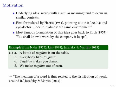
Underlying idea: words with a similar meaning tend to occur insimilar contexts.First formulated by Harris (1954), pointing out that “oculist andeye-doctor . . . occur in almost the same environment”.Most famous formulation of this idea goes back to Firth (1957):“You shall know a word by the company it keeps”.
Example from Nida (1975); Lin (1998); Jurafsky & Martin (2015)(1) a. A bo�le of tesguino is on the table.
b. Everybody likes tesguino.c. Tesguino makes you drunk.d. We make tesguino out of corn.
⇒ “�e meaning of a word is thus related to the distribution of wordsaround it.” Jurafsky & Martin (2015)
4 / 22
Word vectors
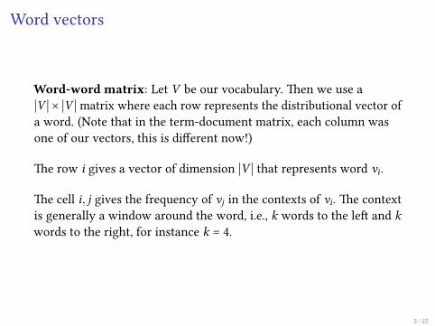
Word-word matrix: Let V be our vocabulary. �en we use a∣V ∣× ∣V ∣ matrix where each row represents the distributional vector ofa word. (Note that in the term-document matrix, each column wasone of our vectors, this is di�erent now!)
�e row i gives a vector of dimension ∣V ∣ that represents word vi.
�e cell i, j gives the frequency of vj in the contexts of vi. �e contextis generally a window around the word, i.e., k words to the le� and kwords to the right, for instance k = 4.
5 / 22
Word vectors
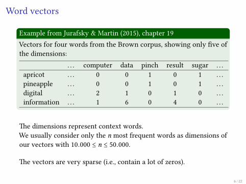
Example from Jurafsky & Martin (2015), chapter 19Vectors for four words from the Brown corpus, showing only �ve ofthe dimensions:
. . . computer data pinch result sugar . . .apricot . . . 0 0 1 0 1 . . .pineapple . . . 0 0 1 0 1 . . .digital . . . 2 1 0 1 0 . . .information . . . 1 6 0 4 0 . . .
�e dimensions represent context words.We usually consider only the n most frequent words as dimensions ofour vectors with 10.000 ≤ n ≤ 50.000.
�e vectors are very sparse (i.e., contain a lot of zeros).
6 / 22
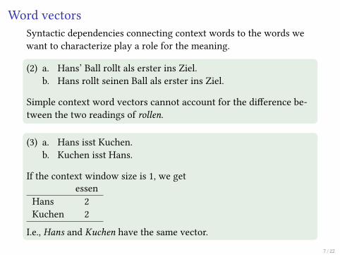
Word vectorsSyntactic dependencies connecting context words to the words wewant to characterize play a role for the meaning.
(2) a. Hans’ Ball rollt als erster ins Ziel.b. Hans rollt seinen Ball als erster ins Ziel.
Simple context word vectors cannot account for the di�erence be-tween the two readings of rollen.
(3) a. Hans isst Kuchen.b. Kuchen isst Hans.
If the context window size is 1, we getessen
Hans 2Kuchen 2
I.e., Hans and Kuchen have the same vector.
7 / 22
Word vectors
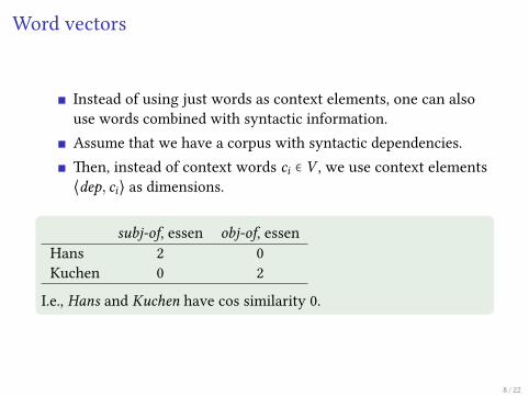
Instead of using just words as context elements, one can alsouse words combined with syntactic information.Assume that we have a corpus with syntactic dependencies.�en, instead of context words ci ∈ V , we use context elements⟨dep, ci⟩ as dimensions.
subj-of, essen obj-of, essenHans 2 0Kuchen 0 2
I.e., Hans and Kuchen have cos similarity 0.
8 / 22
Pointwise mutual information
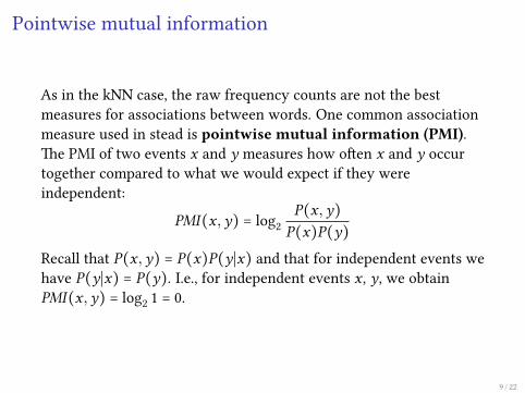
As in the kNN case, the raw frequency counts are not the bestmeasures for associations between words. One common associationmeasure used in stead is pointwise mutual information (PMI).�e PMI of two events x and y measures how o�en x and y occurtogether compared to what we would expect if they wereindependent:
PMI(x,y) = log2P(x,y)
P(x)P(y)Recall that P(x,y) = P(x)P(y∣x) and that for independent events wehave P(y∣x) = P(y). I.e., for independent events x, y, we obtainPMI(x,y) = log2 1 = 0.
9 / 22
Pointwise mutual information
For our speci�c case of vector semantics, we measure the associationbetween a target word w and a context word c as
PMI(w, c) = log2P(w, c)
P(w)P(c)
PMI gives us an estimate of how much more the word w and contextword c co-occur than we would expect by chance.
10 / 22
Pointwise mutual information
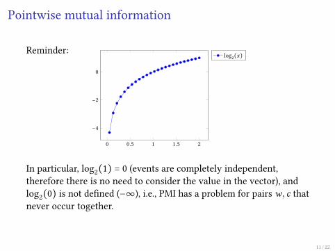
Reminder:
0 0.5 1 1.5 2
−4
−2
0
log2(x)
In particular, log2(1) = 0 (events are completely independent,therefore there is no need to consider the value in the vector), andlog2(0) is not de�ned (−∞), i.e., PMI has a problem for pairs w, c thatnever occur together.
11 / 22
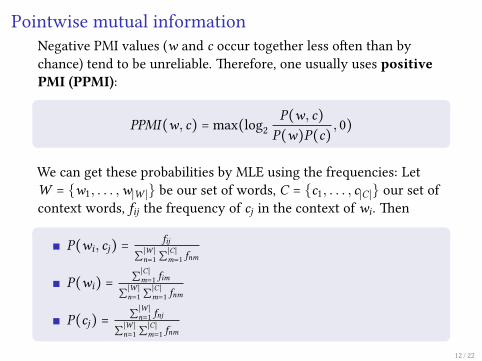
Pointwise mutual informationNegative PMI values (w and c occur together less o�en than bychance) tend to be unreliable. �erefore, one usually uses positivePMI (PPMI):
PPMI(w, c) = max(log2P(w, c)
P(w)P(c) , 0)
We can get these probabilities by MLE using the frequencies: LetW = {w1, . . . ,w∣W ∣} be our set of words, C = {c1, . . . , c∣C∣} our set ofcontext words, fij the frequency of cj in the context of wi. �en
P(wi, cj) = fij∑∣W ∣n=1∑
∣C∣m=1 fnm
P(wi) = ∑∣C∣m=1 fim
∑∣W ∣n=1∑
∣C∣m=1 fnm
P(cj) = ∑∣W ∣n=1 fnj
∑∣W ∣n=1∑
∣C∣m=1 fnm
12 / 22
Pointwise mutual information
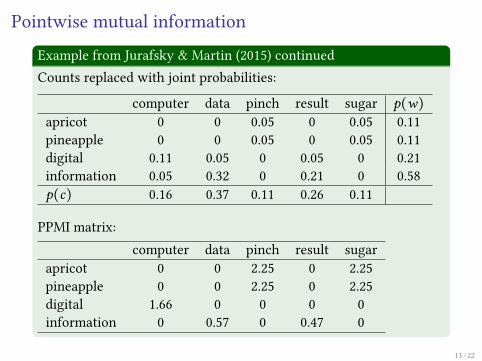
Example from Jurafsky & Martin (2015) continuedCounts replaced with joint probabilities:
computer data pinch result sugar p(w)apricot 0 0 0.05 0 0.05 0.11pineapple 0 0 0.05 0 0.05 0.11digital 0.11 0.05 0 0.05 0 0.21information 0.05 0.32 0 0.21 0 0.58p(c) 0.16 0.37 0.11 0.26 0.11
PPMI matrix:computer data pinch result sugar
apricot 0 0 2.25 0 2.25pineapple 0 0 2.25 0 2.25digital 1.66 0 0 0 0information 0 0.57 0 0.47 0
13 / 22
Pointwise mutual information
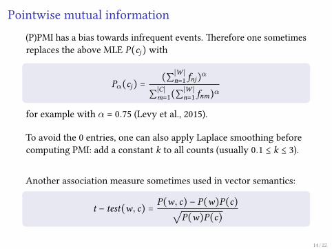
(P)PMI has a bias towards infrequent events. �erefore one sometimesreplaces the above MLE P(cj) with
Pα(cj) =(∑∣W ∣n=1 fnj)α
∑∣C∣m=1(∑∣W ∣n=1 fnm)α
for example with α = 0.75 (Levy et al., 2015).
To avoid the 0 entries, one can also apply Laplace smoothing beforecomputing PMI: add a constant k to all counts (usually 0.1 ≤ k ≤ 3).
Another association measure sometimes used in vector semantics:
t − test(w, c) = P(w, c) − P(w)P(c)√P(w)P(c)
14 / 22
From sparse vectors to dense embeddings
So far, our vectors are high-dimensional and sparse. Singular valuedecomposition (SVD) is a classic method for generating densevectors.
Idea:
Change the dimensions such that they are still orthogonal toeach other.�e new dimensions are such that the �rst describes the largestamount of variance in the data, the second the second largevariance amount etc.�en, instead of keeping all the m dimensions resulting fromthis, we only keep the �rst k.
15 / 22
From sparse vectors to dense embeddings
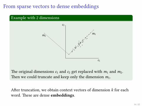
Example with 2 dimensionsc2
c1
m1m2
⋅⋅⋅⋅
⋅
⋅
⋅⋅⋅⋅⋅⋅⋅⋅⋅⋅⋅⋅⋅⋅⋅⋅⋅⋅⋅⋅⋅⋅⋅⋅⋅⋅⋅⋅⋅⋅⋅⋅⋅⋅ ⋅⋅
�e original dimensions c1 and c2 get replaced with m1 and m2.�en we could truncate and keep only the dimension m1.
A�er truncation, we obtain context vectors of dimension k for eachword. �ese are dense embeddings.
16 / 22
From sparse vectors to dense embeddings
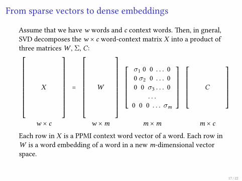
Assume that we have w words and c context words. �en, in gneral,SVD decomposes the w × c word-context matrix X into a product ofthree matrices W , Σ, C:⎡⎢⎢⎢⎢⎢⎢⎢⎢⎢⎢⎢⎢⎢⎢⎣
X
⎤⎥⎥⎥⎥⎥⎥⎥⎥⎥⎥⎥⎥⎥⎥⎦
=
⎡⎢⎢⎢⎢⎢⎢⎢⎢⎢⎢⎢⎢⎢⎢⎣
W
⎤⎥⎥⎥⎥⎥⎥⎥⎥⎥⎥⎥⎥⎥⎥⎦
⎡⎢⎢⎢⎢⎢⎢⎢⎢⎢⎣
σ1 0 0 . . . 00 σ2 0 . . . 00 0 σ3 . . . 0
. . .0 0 0 . . . σm
⎤⎥⎥⎥⎥⎥⎥⎥⎥⎥⎦
⎡⎢⎢⎢⎢⎢⎢⎢⎢⎢⎣
C
⎤⎥⎥⎥⎥⎥⎥⎥⎥⎥⎦
w × c w ×m m ×m m × c
Each row in X is a PPMI context word vector of a word. Each row inW is a word embedding of a word in a new m-dimensional vectorspace.
17 / 22
From sparse vectors to dense embeddings
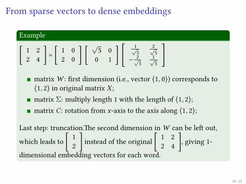
Example
[ 1 22 4 ] = [ 1 0
2 0 ] [√5 00 1 ]
⎡⎢⎢⎢⎢⎣
1√
52√
5− 2√
51√
5
⎤⎥⎥⎥⎥⎦
matrixW : �rst dimension (i.e., vector ⟨1, 0⟩) corresponds to⟨1, 2⟩ in original matrix X ;matrix Σ: multiply length 1 with the length of ⟨1, 2⟩;matrix C: rotation from x-axis to the axis along ⟨1, 2⟩;
Last step: truncation.�e second dimension inW can be le� out,
which leads to [ 12 ] instead of the original [ 1 2
2 4 ], giving 1-dimensional embedding vectors for each word.
18 / 22
From sparse vectors to dense embeddings
Other popular methods for generating dense embeddings areskip-gram and continuous bag of words (CBOW).Both of them are implemented in the word2vec package Mikolovet al. (2013).
19 / 22
Evaluating vector models
One common way to test distributional vector models is to evaluatetheir performance on similarity. Some datasets one can evaluate on:
WordSim-353, a set of ratings from 0 to 10 of the similarity of353 noun pairsSimLex includes both concrete and abstract noun and verbpairs.�e TOEFL dataset is a set of 80 questions, each consistingof a target word and 4 word choices. E.g., Levied is closest inmeaning to: imposed, believed, requested, correlated
�e Stanford Contextual Word Similarity (SCWS) datasetgives human judgements on 2,003 pairs of words in their sen-tential context.
20 / 22
References
Firth, J. R. 1957. A synopsis of linguistic theory 1930–1955. In Studies in linguisticanalysis, Philological Society. Reprinted in Palmer, F. (ed.) 1968. Selected Papers ofJ. R. Firth. Longman, Harlow.
Harris, Z. S. 1954. Distributional structure. Word 10. 146–162. Reprinted in J. Fodorand J. Katz,�e Structure of Language, Prentice Hall, 1964 and in Z. S. Harris,Papers in Structural and Transformational Linguistics, Reidel, 1970, 775–794.
Jurafsky, Daniel & James H. Martin. 2015. Speech and language processing. anintroduction to natural language processing, computational linguistics, andspeech recognition. Dra� of the 3rd edition.
Levy, Omer, Yoav Goldberg & Ido Dagan. 2015. Improving distributional similaritywith lessons learned from word embeddings. Transactions of the Association forComputational Linguistics 3. 211–225. https://tacl2013.cs.columbia.edu/ojs/index.php/tacl/article/view/570.
Lin, Dekang. 1998. Automatic retrieval and clustering of similar words. InProceedings of the 17th international conference on computational linguistics -volume 2 COLING ’98, 768–774. Stroudsburg, PA, USA: Association forComputational Linguistics. doi:10.3115/980432.980696.http://dx.doi.org/10.3115/980432.980696.
21 / 22
Mikolov, T., K. Chen, G. Corrado & J. Dean. 2013. E�cient estimation of wordrepresentations in vector space. ICLR .
Nida, E. A. 1975. Componential analysis of meaning: An introduction to semanticstructures. �e Hague: Mouton.
22 / 22