Machine Learning for Signal Processing

Lecture 1: IntroductionRepresenting sound and images

Class 1. 29 Aug 2017

Instructor: Bhiksha Raj

11-755/18-797 1

Nota Bene

• This course is also being taught at Johns Hopkins University

– Najim Dehak

– Materials and Lectures are shared

– Projects may be collaborative

– Website:

• TBD

11-755/18-797 2

What is a signal

• A mechanism for conveying information

– Semaphores, gestures, traffic lights..

• In Electrical Engineering: currents, voltages

• Digital signals: Ordered collections of numbers that convey information

– from a source to a destination

– about a real world phenomenon

• Sounds, images

11-755/18-797 3

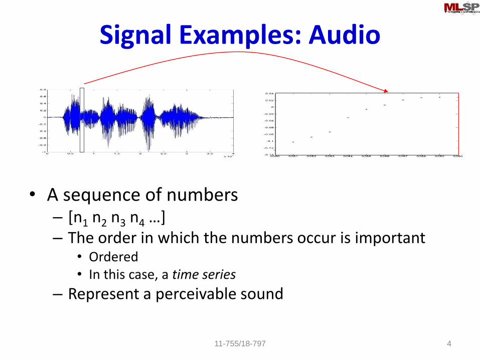
Signal Examples: Audio

• A sequence of numbers– [n1 n2 n3 n4 …]– The order in which the numbers occur is important

• Ordered• In this case, a time series

– Represent a perceivable sound

11-755/18-797 4

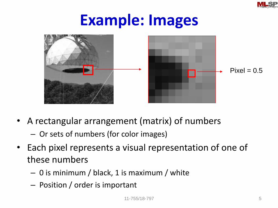
Example: Images

• A rectangular arrangement (matrix) of numbers

– Or sets of numbers (for color images)

• Each pixel represents a visual representation of one of these numbers

– 0 is minimum / black, 1 is maximum / white

– Position / order is important

11-755/18-797 5

Pixel = 0.5

Example: Biosignals

• Biosignals

– MRI: “k-space” 3D Fourier transform

• Invert to get image

– EEG: Many channels of brain electrical activity

– ECG: Cardiac activity

– OCT, Ultrasound, Echo cardiogram: Echo-based imaging

– Others..6

MRI

EEG ECG

Optical Coherence Tomography

11-755/18-797

Financial Data

• Stocks, options, other derivatives

• Analyze trends and make predictions

• Special Issues on Signal Processing Methods in Finance

and Electronic Trading from various journals

11-755/18-797 7

Many others

• Network data..

• Weather..

• Any stochastic time series

• Etc.

11-755/18-797 8

What is Signal Processing• Acquisition, Analysis, Interpretation, and Manipulation of

signals.– Acquisition:

• Sampling, sensing

– Analysis:• Decomposition: Separating signals into basic “building” blocks

– Manipulation:• Denoising• Coding: GSM, Jpeg, Mpeg, Ogg Vorbis

– Interpretation:• Detection: Radars, Sonars• Pattern matching: Biometrics, Iris recognition, finger print recognition• Prediction: Financial prediction, speech coding, etc.

– Etc.

• Boundaries between these categories of operations are fuzzy

11-755/18-797 9

The Tasks in a typical Signal Processing Paradigm

• Capture: Recovery, enhancement

• Channel: Coding-decoding, compression-decompression, storage

• Regression: Prediction, classification

11-755/18-797 10

SignalCapture

FeatureExtraction

ChannelModeling/Regression

sensor

What is Machine Learning

• The science that deals with the development of algorithms that can learn from data

– Learning the structure of data• Feature extraction

– Learning patterns in data

• Automatic text categorization; Market basket analysis

– Learning to classify between different kinds of data

• Is that picture a flower or not?

– Learning to predict data

• Weather prediction, movie recommendation

• Statistical analysis and pattern recognition when performed by a computer scientist..

11-755/18-797 11

MLSP• Application of Machine Learning techniques to the

analysis of signals

• Can be applied to each component of the chain

11-755/18-797 12

SignalCapture

FeatureExtraction

ChannelModeling/Regression

sensor

MLSP• Application of Machine Learning techniques to the

analysis of signals

• Can be applied to each component of the chain

• Sensing

– Compressed sensing, dictionary based representations

• Denoising

– ICA, filtering, separation

11-755/18-797 13

SignalCapture

FeatureExtraction

ChannelModeling/Regression

sensor

MLSP• Application of Machine Learning techniques to the

analysis of signals

• Can be applied to each component of the chain

• Channel: Compression, coding

11-755/18-797 14

SignalCapture

FeatureExtraction

ChannelModeling/Regression

sensor

MLSP• Application of Machine Learning techniques to the

analysis of signals

• Can be applied to each component of the chain

• Feature Extraction:

– Dimensionality reduction

• Linear models, non-linear models

11-755/18-797 15

SignalCapture

FeatureExtraction

ChannelModeling/Regression

sensor

MLSP• Application of Machine Learning techniques to the

analysis of signals

• Can be applied to each component of the chain

• Classification, Modelling and Interpretation,

Prediction

11-755/18-797 16

SignalCapture

FeatureExtraction

ChannelModeling/Regression

sensor

In this course

• The four “aspects” of MLSP:

– Representation: How best to represent signals for

effective downstream or upstream processing

– Modeling: How to model the systematic and

statistical characteristics of the signal

– Classification: How do we assign a class to the

data?

– Prediction: How do we predict new or unseen

values or attributes of the data

11-755/18-797 17

What we will cover

• Representations: Algebraic methods for extracting information from signals

– Deterministic representations

– Data-driven characterization

• PCA

• ICA

• NMF

• Factor Analysis

• LGMs

11-755/18-797 18

What we will cover

• Representations/Modelling: Learning-based approaches for modeling data

– Dictionary representations

– Sparse estimation

• Sparse and over-complete characterization, Compressed sensing

– Regression

• Modelling: Latent variable characterization

– Clustering, K-means

– Expectation Maximization

– Bayes network models

– Probabilistic Latent Component Analysis

11-755/18-797 19

What we will cover

• Modeling/Prediction: Time Series Models– Markov models and Hidden Markov models– Linear and non-linear dynamical systems

• Kalman filters, particle filtering

• Classification and Prediction:– Binary classification. Meta-classifiers– Factor graphs and related models– Neural networks

• Wish list: Additional topics– Privacy in signal processing– Extreme value theory– Dependence and significance

11-755/18-797 20

Recommended Background

• DSP– Fourier transforms, linear systems, basic statistical signal

processing

• Linear Algebra– Definitions, vectors, matrices, operations, properties

• Probability– Basics: what is an random variable, probability distributions,

functions of a random variable

• Machine learning– Learning, modelling and classification techniques

11-755/18-797 21

11-755/18-797 22

Guest Lectures

• TBD

Schedule of Other Lectures

• Tentative Schedule on Website

• http://mlsp.cs.cmu.edu/courses/fall2017

11-755/18-797 23

Grading• Mini quizzes : 25%

– Ten multiple-choice questions on the topics of the week

– Weekly

– Will be open on Friday, closed on Saturday night

• Homework assignments : 50%

– Mini projects

– Will be assigned during course

– Expect five

– You will not catch up if you slack on any homework• Those who didn’t slack will also do the next homework

• Final project: 25%

– Will be assigned early in course

– Dec 7: Poster presentation for all projects, with demos (if possible) • Partially graded by visitors to the poster

11-755/18-797 24

Instructor and TA• Instructor: Prof. Bhiksha Raj

– Room 6705 Hillman Building

– bhiksha@cs.cmu.edu

– 412 268 9826

• TAs: – Yixuan Zhang (yixuanz@andrew)

– Abelino Jimenez (abelinoj@andrew)

– Anurag Kumar (alnu@andrew)

– Davy Uwizera (duwizera@andrew)

• Office Hours:– Instructor: Wednesday, 1-2.30; I also have an open-door policy

– TAs: TBD11-755/18-797 25

Hillman

Windows

My office

Forbes

Additional Administrivia

• Website:– http://mlsp.cs.cmu.edu/courses/fall2017/

– Lecture material will be posted on the day of each class on the website

– Reading material and pointers to additional information will be on the website

• We will use Piazza– Expect an invite to join 11-755/18-797

• Mailing list: Information will be posted

11-755/18-797 26

Continuing..

• Story so far:

– What is a signal

– Some types of signals

– What is SP

– What is ML

• And where does it apply in the SP chain

• Continuing – additional concepts..

– More on signals

– More on what we do with signals

• Representation, Regression, classification, prediction

– And how

• Supervision

11-755/18-797 27

More on Signals

• Principles of signal capture and what the numbers mean

• Explained through examples

– Sound, images

• Signals where the purpose of signal capture is to recreate stimulus

• Signals we emphasize a bit in course

• But also because easily interpretable principles that extend to all signals

– Also MRI

• Illustrates capture in transform domain

11-755/18-797 28

E.g. Audio Signals

• A typical digital audio signal– It’s a sequence of numbers

– Must represent a quantity that enables near-perfect recreation of sound stimulus

11-755/18-797 29

The sound stimulus

• Any sound is a pressure wave: alternating highs and lows of air pressure moving through the air

• When we speak, we produce these pressure waves

– Essentially by producing puff after puff of air

– Any sound producing mechanism actually produces pressure waves

• These pressure waves move the eardrum

– Highs push it in, lows suck it out

– We sense these motions of our eardrum as “sound”

11-755/18-797 30

Pressure highs

Spaces between

arcs show pressure

lows

SOUND PERCEPTION

11-755/18-797 31

Storing pressure waves on a computer

• The pressure wave moves a diaphragm– On the microphone

• The motion of the diaphragm is converted to continuous variations of an electrical signal– Many ways to do this

• A “sampler” samples the continuous signal at regular intervals of time and stores the numbers

11-755/18-797 32

Are these numbers sound?

• How do we even know that the numbers we store on the computer have anything to do with the recorded sound really?– Recreate the sense of sound

• The numbers are used to control the levels of an electrical signal

• The electrical signal moves a diaphragm back and forth to produce a pressure wave– That we sense as sound

11-755/18-797 33

********* ***

**

****

**

** **

*

*

Are these numbers sound?

• How do we even know that the numbers we store on the computer have anything to do with the recorded sound really?– Recreate the sense of sound

• The numbers are used to control the levels of an electrical signal

• The electrical signal moves a diaphragm back and forth to produce a pressure wave– That we sense as sound

11-755/18-797 34

********* ***

**

****

**

** **

*

*

How many samples a second• Convenient to think of sound in terms of

sinusoids with frequency

• Sounds may be modelled as the sum of many sinusoids of different frequencies

– Frequency is a physically motivated unit

– Each hair cell in our inner ear is tuned to specific frequency

• Any sound has many frequency components

– We can hear frequencies up to 16000Hz

• Frequency components above 16000Hz can be heard by children and some young adults

• Nearly nobody can hear over 20000Hz.

11-755/18-797 35

0 10 20 30 40 50 60 70 80 90 100-1

-0.5

0

0.5

1

P

ressure

A sinusoid

Signal representation - Sampling

• Sampling frequency (or sampling rate) refers to the number of samples taken a second

• Sampling rate is measured in Hz

– We need a sample rate twice as high as the highest frequency we want to represent (Nyquist freq)

• For our ears this means a sample rate of at least 40kHz

– Because we hear up to 20kHz

11-755/18-797 36

**

****

**

*****

Time in secs.

Aliasing• Low sample rates result in aliasing

– High frequencies are misrepresented

– Frequency f1 will become (sample rate – f1 )

– In video also when you see wheels go backwards

11-755/18-797 37

Aliasing examples

11-755/18-797 38

Time

Fre

quency

0 0.1 0.2 0.3 0.4 0.5 0.6 0.7 0.8 0.90

0.5

1

1.5

2

x 104

Time

Fre

quency

0 0.1 0.2 0.3 0.4 0.5 0.6 0.7 0.8 0.90

2000

4000

6000

8000

10000

Time

Fre

quency

0 0.1 0.2 0.3 0.4 0.5 0.6 0.7 0.8 0.90

1000

2000

3000

4000

5000

Sinusoid sweeping from 0Hz to 20kHz

44.1kHz SR, is ok 22kHz SR, aliasing! 11kHz SR, double aliasing!

On real sounds

at 44kHz

at 22kHz

at 11kHz

at 5kHz

at 4kHz

at 3kHz

On videoOn images

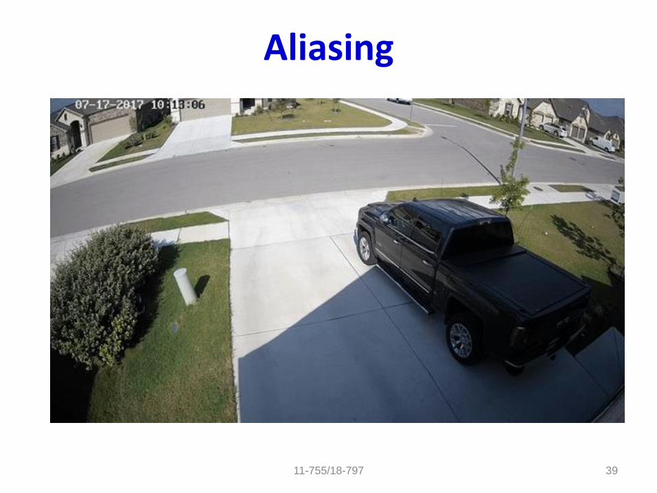
Aliasing

11-755/18-797 39

Aliasing examples

11-755/18-797 40

Time

Fre

quency

0 0.1 0.2 0.3 0.4 0.5 0.6 0.7 0.8 0.90

0.5

1

1.5

2

x 104

Time

Fre

quency

0 0.1 0.2 0.3 0.4 0.5 0.6 0.7 0.8 0.90

2000

4000

6000

8000

10000

Time

Fre

quency

0 0.1 0.2 0.3 0.4 0.5 0.6 0.7 0.8 0.90

1000

2000

3000

4000

5000

Sinusoid sweeping from 0Hz to 20kHz

44.1kHz SR, is ok 22kHz SR, aliasing! 11kHz SR, double aliasing!

On real sounds

at 44kHz

at 22kHz

at 11kHz

at 5kHz

at 4kHz

at 3kHz

On videoOn images

Avoiding Aliasing

• Solution: Filter the signal before sampling it– Cut off all frequencies above sampling.frequency/2

– E.g., to sample at 44.1Khz, filter the signal to eliminate all frequencies above 22050 Hz

• Will only lose information, but not distort existing information11-755/18-797 41

Antialiasing

FilterSampling

Analog signal Digital signal

Time

Fre

quency

0 0.1 0.2 0.3 0.4 0.5 0.6 0.7 0.8 0.90

0.5

1

1.5

2

x 104

Time

Fre

quency

0 0.1 0.2 0.3 0.4 0.5 0.6 0.7 0.8 0.90

1000

2000

3000

4000

5000

44kHz SR, is ok 11kHz SR, antialiased!

Time

0 0.1 0.2 0.3 0.4 0.5 0.6 0.7 0.8 0.90

2000

4000

6000

8000

10000

22kHz SR, antialiased!

Problem 2: Resolution

• Sound is the outcome of a continuous range of variations

– The pressure wave can take any value (within limits)

• A computer has finite resolution

– Numbers can only be stored to finite resolution

– E.g. a 16-bit number can store only 65536 values, while a 4-bit number can store only 16 unique values

• Low-resolution storage results in loss of information

11-755/18-797 42

Storing the signal on a computer

• The original signal

• 8 bit quantization

• 3 bit quantization

• 2 bit quantization

• 1 bit quantization

11-755/18-797 43

Tom Sullivan Says his Name

• 16 bit sampling

• 5 bit sampling

• 4 bit sampling

• 3 bit sampling

• 1 bit sampling

11-755/18-797 44

A Schubert Piece

11-755/18-797 45

• 16 bit sampling

• 5 bit sampling

• 4 bit sampling

• 3 bit sampling

• 1 bit sampling

Lessons (for any signal)

• Transduce signal in meaningful manner– For sound and images, must be able to recreate original stimulus from

signal

• Sample fast enough to capture highest frequency variations

• Store with sufficient resolution

• For audio– Common sample rates

• For speech 8kHz to 16kHz

• For music 32kHz to 44.1kHz

• Pro-equipment 96kHz

– Common bit resolution

• 12-bit equivalent for speech

• 16 bits for high-fidelity speech

• 24 bits for music

11-755/18-797 46

Images

11-755/18-797 47

Images

11-755/18-797 48

The Eye

11-755/18-797 49

Basic Neuroscience: Anatomy and Physiology Arthur C. Guyton, M.D. 1987 W.B.Saunders Co.

Retina

The Retina

11-755/18-797 50http://www.brad.ac.uk/acad/lifesci/optometry/resources/modules/stage1/pvp1/Retina.html

Rods and Cones

• Separate Systems

• Rods– Fast

– Sensitive

– Grey scale

– predominate in the periphery

• Cones– Slow

– Not so sensitive

– Fovea / Macula

– COLOR!

11-755/18-797 51

Basic Neuroscience: Anatomy and Physiology Arthur C. Guyton, M.D. 1987 W.B.Saunders Co.

The Eye

• The density of cones is highest at the fovea

– The region immediately surrounding the fovea is the macula• The most important part of your eye: damage == blindness

• Peripheral vision is almost entirely black and white

• Eagles are bifoveate

• Dogs and cats have no fovea, instead they have an elongated slit 52

Three Types of Cones (trichromatic vision)

11-755/18-797 53

Wavelength in nm

Norm

aliz

ed r

eponse

Trichromatic Vision

• So-called “blue” light sensors respond to an entire range of frequencies

– Including in the so-called “green” and “red” regions

• The difference in response of “green” and “red” sensors is small

– Varies from person to person

• Each person really sees the world in a different color

– If the two curves get too close, we have color blindness

• Ideally traffic lights should be red and blue11-755/18-797 54

White Light

11-755/18-797 55

Response to White Light

?

11-755/18-797 56

Response to White Light

11-755/18-797 57

Response to Sparse Light

11-755/18-797 58

?

Response to Sparse Light

11-755/18-797 59

Response to Sparse Light

11-755/18-797 60

Digital Capture of Images

• Lens projects image on sensor

– Typically CCD or CMOS

• Sensor comprises sensing elements of 3 colors

– Different strategies for arrangement of color sensors

• Limited number of sensing elements

– 200-600 ppi

– The camera generally includes an anti-aliasing filter to eliminate aliasing in the image

11-755/18-797 61

Representing Images

• Utilize trichromatic nature of human vision

– Trigger the three cone types to produce a sensation approximating desired color

• A tetrachromatic animal would be very confused by our computer images

– Some new-world monkeys are tetrachromatic

• The three “chosen” colors are red (650nm), green (510nm) and blue (475nm)

• Can still only represent a small fraction of the 10 million colors that humans

can sense

11-755/18-797 62

Computer Images: Grey Scale

11-755/18-797 63

Picture Element (PIXEL)

Position & gray value (scalar)

R = G = B. Only a single number need

be stored per pixel

Signal: Each stored number represents

a single pixel

10

10

What we see What the computer “sees”

11-755/18-797 64

Picture Element (PIXEL)Position & color value (red, green, blue)

Color Images

11-755/18-797 65

Signal: Each triad of stored numbers

represents a single pixel

RGB Representation

11-755/18-797 66

original

R

B

G

R

B

G

Quantization and Saturation

• Captured images are typically quantized to 8 bits

• 8-bits is not very much < 1000:1

• Humans can easily accept 100,000:1

• And most cameras will give you only 6-bits anyway…

– Truth in advertising!

11-755/18-797 70

Processing Colour Images

• Typically work only on the Grey Scale image

– Decode image from whatever representation to RGB

– GS = R + G + B

• For specific algorithms that deal with colour, individual colours may be maintained

– Or any linear combination that makes sense may be maintained.

11-755/18-797 71

Signals..

• Speech and Images are examples of signals where the digitized signal is a facsimile of the stimulus to be represented

– Many other signals of this kind, including bio-signals, network traffic, etc.

• Next up : a signal where the digitized signal is nota direct facsimile of the data to be represented

– Signal captured in a transform domain

11-755/18-797 72

Magnetic Resonance Imaging

• Attempts to image interior structure of soft tissue

• Does so by imposing a magnetic field and measuring resonance of protons (Hydrogen atoms)

11-755/18-797 73

Cross-section of a body

• Image changes left to right, top to bottom at different rates at different locations

– Different tissue densities…

– … which show up as a range of “spatial frequencies”11-755/18-797 74

MRI

• Takes slice-wise measurements in the Fourier domain

• A single “gradient field” derives response from a single “spatial frequency” component

– Which can be measured

• Sequence of gradient fields derive resonant response of different spatial frequencies of tissue slice

– Effectively a 2D Fourier transform

• Must invert transform to create image

• “Join” slices for full 3-D reconstruction11-755/18-797 75

What we do with signals

• Have seen examples of signals and caveats of signal capture

• Next: Machine Learning challenges in dealing with the data

11-755/18-797 76

Representation

• Signals can be decomposed into combinations of building blocks– Different signals of any category composed as different combinations of the same building

blocks

– Knowing the composing combination informs us about the properties of the signal

• But requires knowing the building blocks

• Using the wrong building blocks will give us imprecise or meaningless conclusions

• ML challenge: Find building blocks from analysis of signals

– Mathematically: S = f(B,W), find B and W from S

– S = signal, B = building blocks, W = combination parameters, f = combination function

11-755/18-797 77

Modelling

• Signals are produced by processes

– Which are generally partially or fully unknown

• Knowledge of the process is often crucial for additional processing

– Control, prediction, analysis

• ML challenge: Characterizing the process underlying the signal

– Characterization through statistical properties of the signal

– Characterization through an abstract parametric model11-755/18-797 78

Rube Goldberg

Classification

• Signals may arise from different classes of stimuli/processes

• Often needed to identify underlying process/stimulus

• ML challenge: Identify underlying “class” of the signal

11-755/18-797 79

?

Prediction

• Signals can be analyzed to make predictions about the

future of the signal or the underlying process

• ML challenge: How to make the “best” predictions

11-755/18-797 80

Supervision

• Learning representations and modeling are often preliminary steps to classification and prediction

• Can be performed without reference to the actual classification/prediction task

– Unsupervised learning

• Can be explicitly optimized

11-755/18-797 81

Supervision

• Task: Detect if it’s a face

• Unsupervised representation: characterize edges, gradation

– Does not specifically help with problem

• Supervised representation: characterize nose-like features, eyebrow-like features, mouth-like features…

– Better suited to detect faces

11-755/18-797 82

?

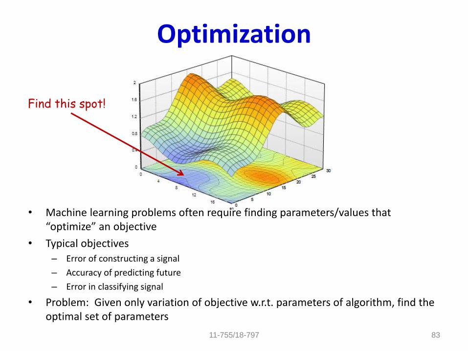
Optimization

• Machine learning problems often require finding parameters/values that “optimize” an objective

• Typical objectives– Error of constructing a signal

– Accuracy of predicting future

– Error in classifying signal

• Problem: Given only variation of objective w.r.t. parameters of algorithm, find the optimal set of parameters

11-755/18-797 83

Find this spot!

Optimization: Formulation• In the majority of machine learning task, a set

of samples is provided

• Supervised learning

• Unsupervised learning (k-mean clustering)

11-755/18-797 84

z1, z2,..., zn

z = (x, y)

h is predictor functionh : X®Y

min imize f (h;(x, y)) = loss function(h(x), y)

z = x Î Âd

h = (m1,....,mk ) Î Âd´k, which correspondsto cluster centers

min imize f ((m1,....,mk );x) = minj

m j - x2

Next Class..

• Review of linear algebra..

11-755/18-797 85