machine learning in computer vision - cgg.mff.cuni.cz
TRANSCRIPT

Machine learning in computer
vision
Lesson 9
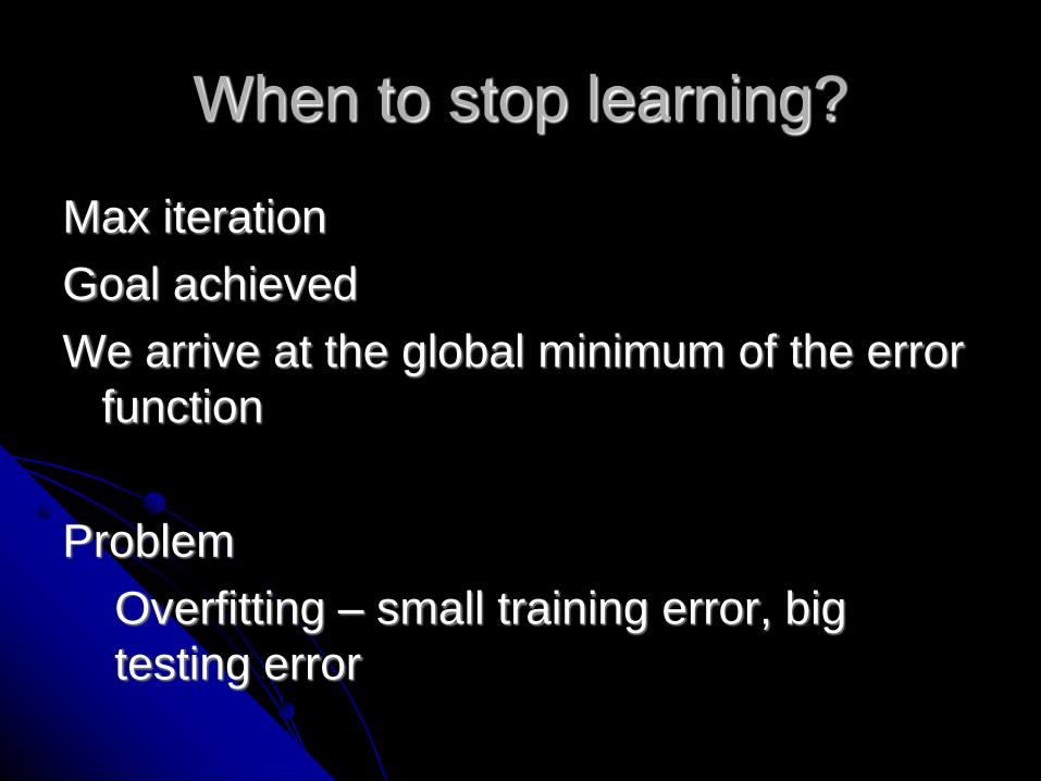
When to stop learning?
Max iteration
Goal achieved
We arrive at the global minimum of the error
function
Problem
Overfitting – small training error, big
testing error
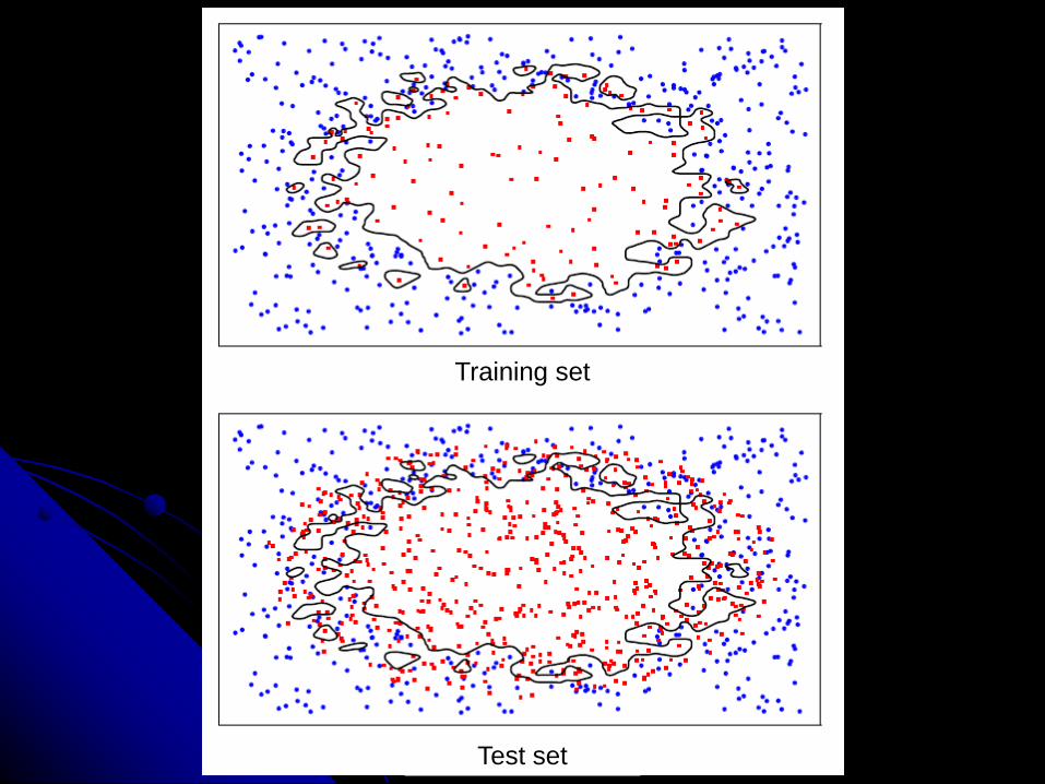
Training set
Test set

Train and validation sets
stop when the validation error starts to
grow
Early stopping

Number of Hidden Layers
# Result
noneOnly capable of representing linear
separable functions or decisions.
1
Can approximate any function that
contains a continuous mapping from one
finite space to another.
2
Can represent an arbitrary decision
boundary to arbitrary accuracy with rational
activation functions and can approximate
any smooth mapping to any accuracy.Jeff Heaton. 2008. Introduction to Neural Networks for Java, 2nd Edition (2nd ed.). Heaton Research, Inc.

Number of neurons in the hidden
layers
rules-of-thumb:
between the size of the input layer and
the size of the output layer.
2/3 the size of the input layer, plus the
size of the output layer.
less than twice the size of the input layer.

Number of parameters
Weights and biases:
[3 x 4] + [4 x 2] = 20 weights
4 + 2 = 6 biases
http://cs231n.github.io/neural-networks-1/

Number of parameters
[3 x 4] + [4 x 4] + [4 x 1] = 12 + 16 + 4 = 32
weights
4 + 4 + 1 = 9 biases

Raw image input
M. Mitchell Waldrop: What are the limits of deep learning?
https://doi.org/10.1073/pnas.1821594116

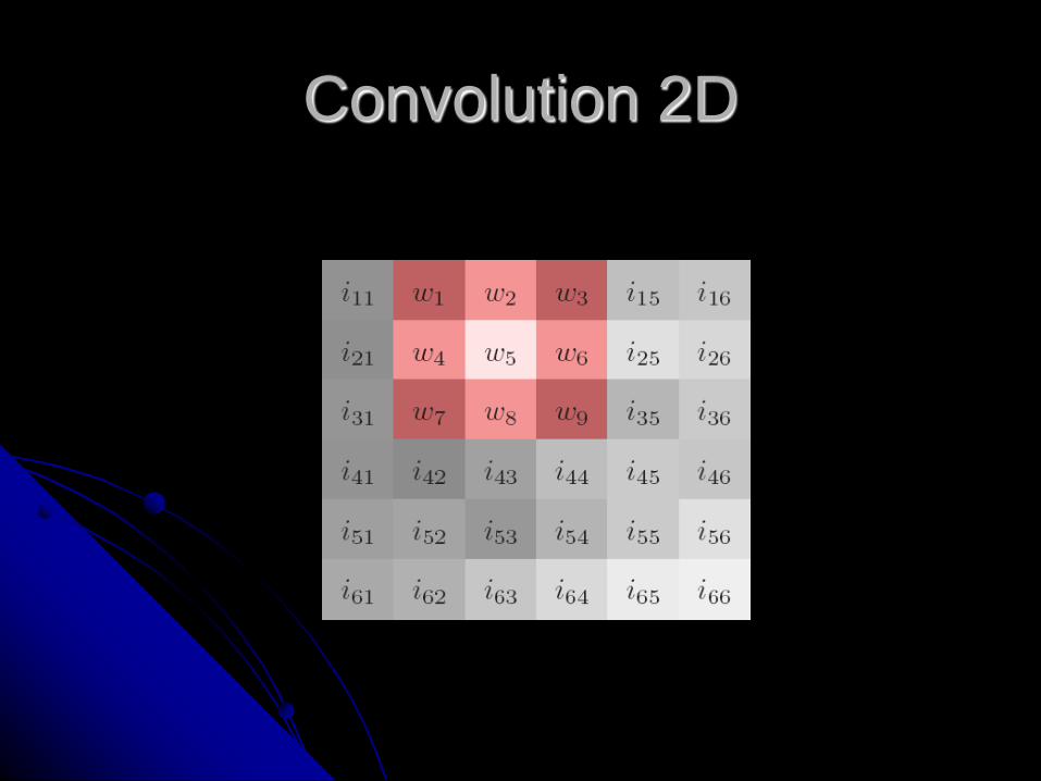
Convolutional neural networks
Discrete 2D convolution
ℎ 𝑘, 𝑙 = 𝐼 ∗ 𝑤 𝑘, 𝑙
=
𝑚=−𝑀
𝑀
𝑛=−𝑁
𝑁
𝐼 𝑚, 𝑛 . 𝑤(𝑘 −𝑚, 𝑙 − 𝑛)

Convolution 2D

Convolution 2D
Convolution 2D

Convolution 2D

Convolution 2D

Convolution 2D

Convolution 2D
h(0,0) = ?ℎ 𝑘, 𝑙 = 𝐼 ∗ 𝑤 𝑘, 𝑙
=
𝑚=−𝑀
𝑀
𝑛=−𝑁
𝑁
𝐼 𝑚, 𝑛 . 𝑤(𝑘 −𝑚, 𝑙 − 𝑛)

Convolution 2D
Border padding

Kernels used in CV
Edge detection
Blurring
Sharpening
Original Blur (with a mean filter)
* =1 1 1
1 1 1
1 1 1
𝟏
𝟗

Convolutional neural networks
𝑓 𝐱 = 𝐰𝑇𝐱 + 𝑏 ℎ 𝑘, 𝑙 = 𝐼 ∗ 𝑤 𝑘, 𝑙

Convolutional neural networks
Convolution layer Non-linear layer Pooling layer

Convolution layer
Image 32x32x3 Filters 5x5x3
1x1xD filter size?

Convolution layer
Stride – next filter position
Size of output: (N-F)/stride+1
stride=1 → 5
stride=2 → 3
stride=3 → 2.33
(N-F+2P)/stride+1

Number of parameters
Weights and biases:
2 x [3 x 3 x 3] = 54 weights
2 biases
http://cs231n.github.io/neural-networks-1/

Non-linear layer
Activation function
ReLU 𝑓 𝑥 = max(0, 𝑥)
And modifications:
Leaky ReLU,
ELU,
SReLU…

Pooling layer
Decreases size, nr. of parameters
Max, average, sum
Size, stride

Receptive field
Input area of a neuron
Layer 3Layer 2Layer 1
https://ujjwalkarn.me/2016/08/11/intuitive-explanation-convnets/

Sample architecture
https://towardsdatascience.com/a-comprehensive-guide-to-convolutional-neural-networks-the-eli5-way-
3bd2b1164a53

Alexnet
Full (simplified) AlexNet architecture:
[227x227x3] INPUT
[55x55x96] CONV1: 96 11x11 filters at stride 4, pad 0
[27x27x96] MAX POOL1: 3x3 filters at stride 2
[27x27x96] NORM1: Normalization layer
[27x27x256] CONV2: 256 5x5 filters at stride 1, pad 2
[13x13x256] MAX POOL2: 3x3 filters at stride 2
[13x13x256] NORM2: Normalization layer
[13x13x384] CONV3: 384 3x3 filters at stride 1, pad 1
[13x13x384] CONV4: 384 3x3 filters at stride 1, pad 1
[13x13x256] CONV5: 256 3x3 filters at stride 1, pad 1
[6x6x256] MAX POOL3: 3x3 filters at stride 2
[4096] FC6: 4096 neurons
[4096] FC7: 4096 neurons
[1000] FC8: 1000 neurons (class scores)

CNN usage I
Classifier:
classify new images
Standalone Feature Extractor:
pre-process images and extract relevant
features.
https://machinelearningmastery.com/how-to-use-transfer-learning-when-developing-convolutional-neural-
network-models/

CNN usage II
Integrated Feature Extractor:
integrated into a new model, but layers of the
pre-trained model are frozen during training
Weight Initialization:
integrated into a new model, and the layers of
the pre-trained model are trained with the new
model

Unsupervised methods

Unsupervised methods
Definition 1
Supervised: human effort involved
Unsupervised: no human effort
Definition 2
Supervised: learning conditional distribution
P(Y|X), X: features, Y: classes
Unsupervised: learning distribution P(X), X:
features
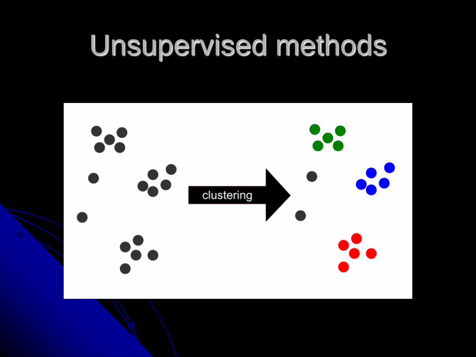
Unsupervised methods

Clustering methods
Hierarchical clustering
Single
link
Complete
link
Average
link
Nonhierarchical clustering
K-meansKohonen neural
networks (SOM)
Fuzzy clustering
Unsupervised methods

Clustering
Nonhierarchical – the space is divided into
one set of clusters

Clustering
Hierarchical – levels of clusters form a tree
structure

Clustering
2 approaches
Agglomerative (Bottom-up)
Divisive (Top-down)

Clustering
Hard vs. Soft
Hard: same object can only belong to single
cluster
Soft: same object can belong to different
clusters
E.g. Gaussian mixture model

Hierarchical methods

Dendrogram
A binary tree that shows how clusters are
merged/split hierarchically
Each node on the tree is a cluster; each leaf node
is a singleton cluster
41

Dendrogram
A clustering of the data objects is obtained by
cutting the dendrogram at the desired level, then
each connected component forms a cluster
42

Dendrogram
A clustering of the data objects is obtained by
cutting the dendrogram at the desired level, then
each connected component forms a cluster
43

Divisive approach
Put all object into one cluster
REPEAT
Pick the cluster to split
Split the cluster
UNTIL individual objects
or desired number of clusters

DIANA (Divisive Analysis)
Introduced in Kaufmann and Rousseeuw
(1990)
Basic algorithm for divisive clustering

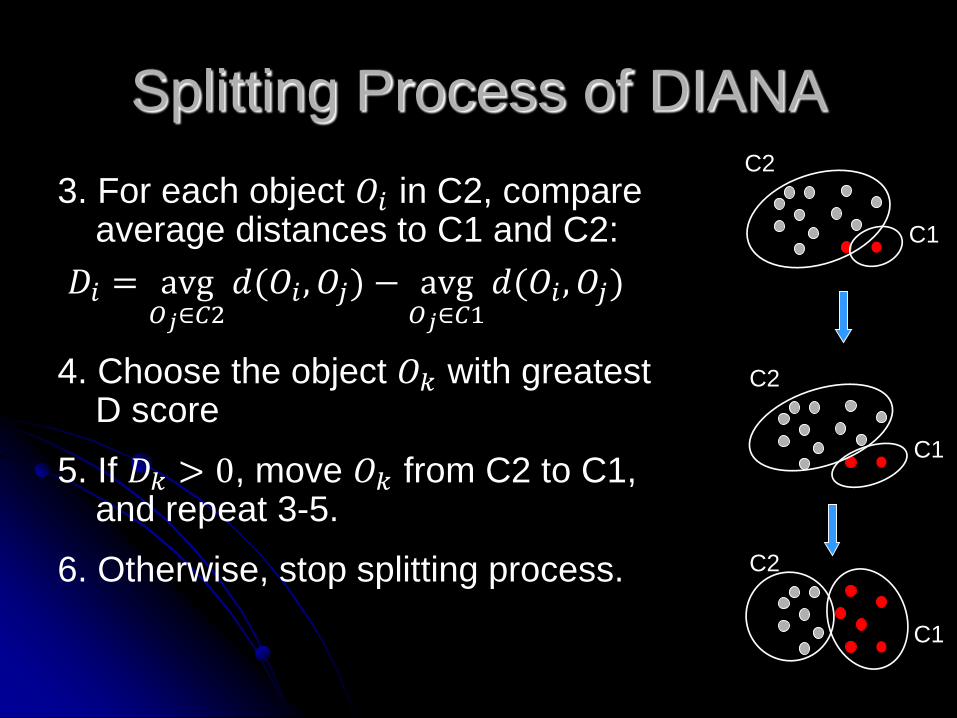
Splitting Process of DIANA
Initialization:
1. Choose the object O which is most
dissimilar to other objects in C
2. Let C1={O}, C2=C-C1
C C2
C1
Splitting Process of DIANAC2
C1
C2
C1
C2
C1
3. For each object 𝑂𝑖 in C2, compare average distances to C1 and C2:
𝐷𝑖 = avg𝑂𝑗∈𝐶2
𝑑(𝑂𝑖 , 𝑂𝑗) − avg𝑂𝑗∈𝐶1
𝑑(𝑂𝑖 , 𝑂𝑗)
4. Choose the object 𝑂𝑘 with greatest D score
5. If 𝐷𝑘 > 0, move 𝑂𝑘 from C2 to C1, and repeat 3-5.
6. Otherwise, stop splitting process.

Principal Directions Divisive
Partitioning
1. Find the principal axis
2. Split point at mean projection
3. Find new centroids

mean
Principal axis
Splitting hyperplane
1. Find the principal axis
2. Split point at mean projection
3. Find new centroids

Principal Directions Divisive
Partitioning
Improvements exist
Tasoulis, S. K., Tasoulis, D. K., and Plagianakos, V. P. (2010). Enhancing principal direction divisive
clustering. Pattern Recognition, Vol. 43,

Median cut
Idea – the prototypes of clusters represent the same number of objects
The prototype = the mean
1. Find the smallest box which contains all the objects
2. Sort the enclosed objects along the longest axis of the box (variance)
3. Split the box into 2 regions at median of the sorted list
4. Repeat the above process until the space has been divided into K regions

Median Cut

4
8
32
256

Agglomerative clustering
Individual objects form clusters
REPEAT
Merge 2 closest clusters (depends on metrics)
UNTIL 1 cluster containing all objects
or desired number of clusters

Agglomerative clustering
Liang Shan: Clustering Techniques and Applications to Image Segmentation

Agglomerative clustering
1st iteration
1

Agglomerative clustering
2nd iteration
1 2

Agglomerative clustering
3rd iteration
1 23
Agglomerative clustering
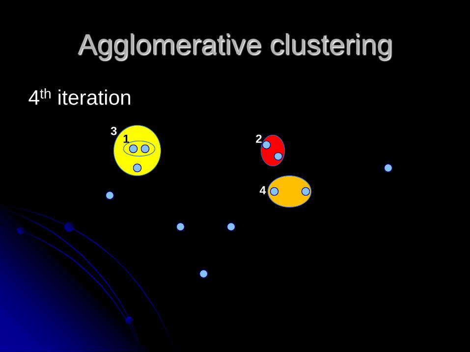
4th iteration
1 23
4
Agglomerative clustering
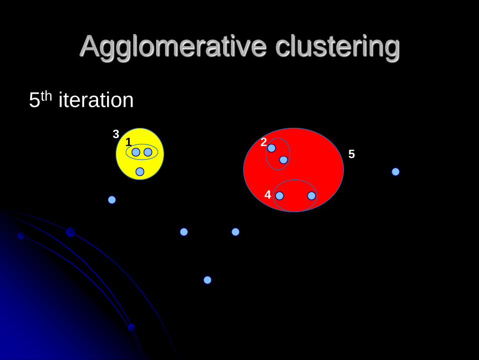
5th iteration
1 23
4
5
Agglomerative clustering
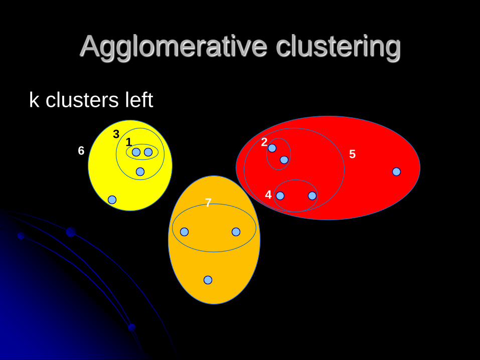
k clusters left
1 23
4
69
5
7
8

Cluster distance
single-link:
Distance of the closest points from A and B
complete-link: Distance of the furthest points from A and B
centroid-link: Distance of the centroids
average-link: Average distance between
pairs of points from A and B

Ward’s method
Merge clusters with minimal merge cost:
𝐶𝐴,𝐵 =𝑁𝐴𝑁𝐵𝑁𝐴 +𝑁𝐵
𝑐𝐴 − 𝑐𝐵2
𝑁𝑘 number of objects in cluster K
𝑐𝑘 cluster centroid
J.H. Ward (1963): Hierarchical grouping to optimize an objective function, J. Am. Statist. Assoc. 58

Example of cost calculations
56
a b c
na = 1
nb = 9nc = 3
da,b=32,40 db,c=56,25
40.323610
936
91
91,
baMergeCost
25.562512
2725
93
93,
cbMergeCost

Hierarchical Clustering: Comparison
Group Average
Ward’s Method
1
2
3
4
5
61
2
5
3
4
MIN MAX
1
2
3
4
5
6
1
2
5
34
1
2
3
4
5
6
1
2 5
3
41
2
3
4
5
6
1
2
3
4
5

Iterative shrinking
Individual objects form clustersREPEAT
Select cluster to remove (smallest removal cost)Repartition the object to the nearby clusters
UNTIL 1 cluster containing all objectsor desired number of clusters
𝐶𝐴 =
𝑥𝑖∈𝐴
𝑁𝑄𝑖𝑁𝑄𝑖 + 1
𝑑 𝑥𝑖 , 𝑐𝑄𝑖 − 𝑑(𝑥𝑖 , 𝑐𝐴)
𝑄𝑖 nearest cluster for object 𝑥𝑖 having the minimal merge costPasi Fränti, Olli Virmajoki (2006): Iterative shrinking method for clustering problems, Pattern Recognition, Volume 39

Shrinking
Code vectors: Training vectors:
Before cluster removal After cluster removal
Vector to be removed
Remaining vectors
Training vectors of the cluster to be removed
Other training vectors
S2
S3
S4
S5
S1
x
+
+ ++
++
+
+
+
x x
x
x
x+
+
+ ++
+
+
+ +
+
+
+
++
+
+ +
+
+ ++
+
+
+
+
x x
x
x
x+
+
+ ++
+
+
+ +
+
+
++
+
+ +
+
+
+