Decision TreesApplied Machine Learning: Unit 1, Lecture 3

Anantharaman Narayana Iyer

narayana dot Anantharaman at gmail dot com

13 Jan 2016

References

• Pattern Recognition and Machine Learning by Christopher Bishop

• Machine Learning, T Mitchell

• CMU Videos Prof T Mitchell

• Introduction to Machine Learning, Alpaydin

• Article by Christopher Roach

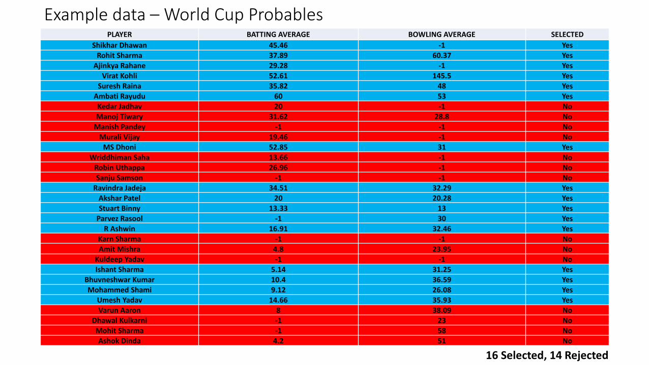
Example data – World Cup ProbablesPLAYER BATTING AVERAGE BOWLING AVERAGE SELECTED

Shikhar Dhawan 45.46 -1 Yes

Rohit Sharma 37.89 60.37 Yes

Ajinkya Rahane 29.28 -1 Yes

Virat Kohli 52.61 145.5 Yes

Suresh Raina 35.82 48 Yes

Ambati Rayudu 60 53 Yes

Kedar Jadhav 20 -1 No

Manoj Tiwary 31.62 28.8 No

Manish Pandey -1 -1 No

Murali Vijay 19.46 -1 No

MS Dhoni 52.85 31 Yes

Wriddhiman Saha 13.66 -1 No

Robin Uthappa 26.96 -1 No

Sanju Samson -1 -1 No

Ravindra Jadeja 34.51 32.29 Yes

Akshar Patel 20 20.28 Yes

Stuart Binny 13.33 13 Yes

Parvez Rasool -1 30 Yes

R Ashwin 16.91 32.46 Yes

Karn Sharma -1 -1 No

Amit Mishra 4.8 23.95 No

Kuldeep Yadav -1 -1 No

Ishant Sharma 5.14 31.25 Yes

Bhuvneshwar Kumar 10.4 36.59 Yes

Mohammed Shami 9.12 26.08 Yes

Umesh Yadav 14.66 35.93 Yes

Varun Aaron 8 38.09 No

Dhawal Kulkarni -1 23 No

Mohit Sharma -1 58 No

Ashok Dinda 4.2 51 No

16 Selected, 14 Rejected

45.46, 100

37.89, 60.37

29.28, 100 52.61, 100

35.82, 48

60, 53

20, 100

31.62, 28.8

0, 100 19.46, 100

52.85, 31

13.66, 100 26.96, 1000, 100

34.51, 32.29

20, 20.28

13.33, 13

0, 3016.91, 32.46

0, 100

4.8, 23.95

0, 100

5.14, 31.25

10.4, 36.59

9.12, 26.08

14.66, 35.938, 38.09

0, 23

0, 58

4.2, 51

0

20

40

60

80

100

120

0 10 20 30 40 50 60 70

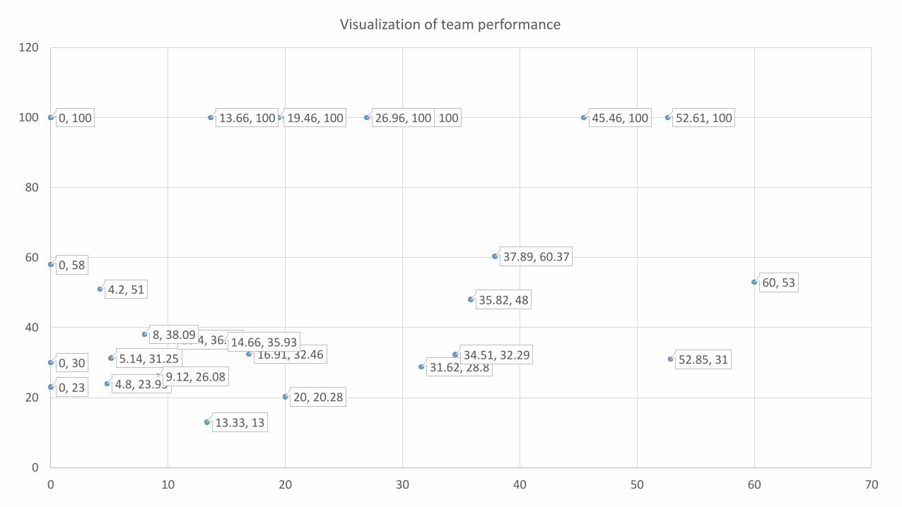
Visualization of team performance

Decision Tree Model Example

θ11 θ12

θ21

θ22

In the fig, X axis represents batting average, Y the bowling average.

Roles: Batsman, Bowler, All rounder

Refer the diagram on the board.

Principle: Build the tree, minimize error at each leaf

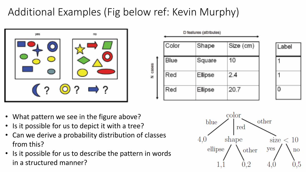
Additional Examples (Fig below ref: Kevin Murphy)

• What pattern we see in the figure above? • Is it possible for us to depict it with a tree?• Can we derive a probability distribution of classes

from this?• Is it possible for us to describe the pattern in words

in a structured manner?

Additional Examples (Fig below ref: Kevin Murphy)

• What pattern we see in the figure above? • Is it possible for us to depict it with a tree?• Can we derive a probability distribution of classes

from this?• Is it possible for us to describe the pattern in words

in a structured manner?

Recall: Function Approximation

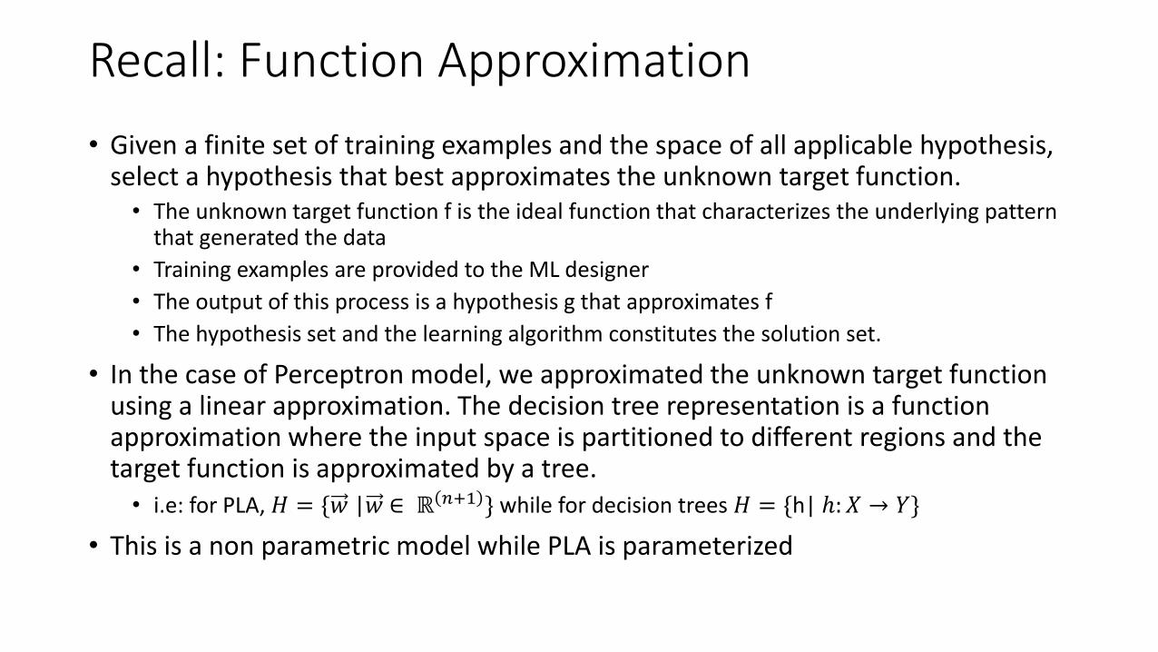
• Given a finite set of training examples and the space of all applicable hypothesis, select a hypothesis that best approximates the unknown target function.• The unknown target function f is the ideal function that characterizes the underlying pattern

that generated the data

• Training examples are provided to the ML designer

• The output of this process is a hypothesis g that approximates f

• The hypothesis set and the learning algorithm constitutes the solution set.

• In the case of Perceptron model, we approximated the unknown target function using a linear approximation. The decision tree representation is a function approximation where the input space is partitioned to different regions and the target function is approximated by a tree.• i.e: for PLA, 𝐻 = {𝑤 |𝑤 ∈ ℝ 𝑛+1 } while for decision trees 𝐻 = {h| ℎ: 𝑋 → 𝑌}

• This is a non parametric model while PLA is parameterized

Decision Tree Representation• The decision tree represents a function that takes a vector of attributes as input and returns

a decision as the single output value.• E.g Input = Medical test results, Output = Normal or Emergency

• i.e. Input = (a1, a2, ….an), Output = y

• The input and output values can be discrete or continuous. • In our discussion today we will consider Boolean output values (Selected, Rejected) and real valued

inputs that can be discretized (Batting average, Bowling Average)

• Each internal node: Test one discrete valued attribute Xi

• Each edge from the node: Selects one value that Xi can take

• Each leaf node: predict Y

• Expressiveness: • The target attribute is true iff the input attributes satisfy one of the paths leading to a leaf that is labelled

true.

• Each path is a conjunction of attribute-value tests

• Whole expression is equivalent to Disjunctive Normal Form – i.e, any function in the propositional logic can be represented by the decision tree.

Exercise

• Suppose we have a feature vector: (X1, X2, ….Xn) how to represent:

• Y = X1 AND X2 ?

• Y = X1 OR X2 ?

• Y = X2 X5 ∨ X3X4(¬X1)

Example: (Ref T Mitchell)

Hypothesis Space for Decision Trees

• Suppose we have n Boolean attributes (or features). How many different functions are there in this set?

• The above is equal to the number of truth tables we can write down with this input set

• A truth table is a function or a decision tree

• We have 2n rows in such a table

• How many such tables are possible?

Decision Tree• A decision tree constructed for n binary attributes will have 2n entries in

the truth table, if all the combinations of the n attributes are specified. This means there will be 2n leaf nodes, which is exponential in n.

• If every possible combination is specified there is no learning needed. We just need a look up table, which is the truth table for Boolean variables.

• However the training dataset is finite, may be noisy and hence generalization is needed. That is samples need not be consistent, may be noisy. Training data may be incomplete.

• We need a compact tree for efficiency of computation and representation

• Every decision is not affected by every variables• Relating to the cricket example, we don’t need to worry about the bowling average

for a player if you are considering him for the role of a batsman

• Many variables become don’t care and we can utilize this aspect to build a compact tree

Inducing a decision tree from examples

• Our goal is to automatically output a tree given the data• This process is also called inducing a tree from the given data

• Consider the cricket example. We need a system that given this data, learns the underlying selection pattern and can be used to classify future instances.

• As searching through the hypothesis space is intractable, we need a way of producing the tree that can be used as a classifier

• A greedy algorithm ID3 is one of the approaches we will discuss

Running ExamplePrice Range Definitions:<20K 120K – 40K 2>40K 3

Key Questions are:1. Given the training dataset as above, what is our algorithm to build a tree?

• What is the criteria to choose the attributes for the internal nodes?• Given such a criteria, how to choose the attributes for the internal nodes?

2. When an unseen new instance is presented, how does this classifier infer?3. How do we analyse the performance of the generated tree against test data?

• Are the training instances provided in the dataset adequate? How do we know?• How sensitive the classifier is to the changes in the training examples?

SNoBrand Product Cores Memory Size Camera Price Code

1Apple iPhone 4s 2 8 3.5 8 19899 1

2Apple iPhone 5s 2 16 4 8 39899 2

3Apple iPhone 6 plus 2 64 5.5 8 71000 3

4Samsung Galaxy Grand 2 4 8 5.25 8 15290 1

5Samsung Galaxy S 4 8 16 5 13 25999 2

6Samsung Galaxy Note 4 4 32 5.7 16 54999 3

7Samsung Galaxy S 5 8 16 5.1 16 32999 2

8Micromax Canvas Doodle A111 4 4 5.3 8 14999 1

9Motorola Moto X 2nd Gen 4 16 5.2 13 31999 2

10Motorola Moto G 2nd Gen 4 16 5 8 12999 1

11Google Nexus 6 4 64 6 13 48999 3

Size Range Definitions:< 5 15 – 5.3 2> 5.3 3

Initial distribution: (4, 4, 3)

ID3 AlgorithmID3(Examples, Target_Attribute, Attributes) returns a decision tree T

Create a root node

If all the examples are positive (or negative) return a tree with single node Root labelled positive (or negative)

If Attributes is empty return a tree with single node Root with label = most common value of Target_Attribute in Examples

Otherwise Begin

Let A be best decision attribute for next node

Assign A as the decision attribute for node

For each value vi of A create new descendant of node

Let Examplesvi be the subset of examples that have the value vi for A

If Examplesvi = Empty

Then below this new branch add a leaf node with label = most common value of Target_Attribute in the Examples

Else below this new branch add the sub tree: ID3(Examplesvi , Target_attribute, Attributes – [A])

End

Return root

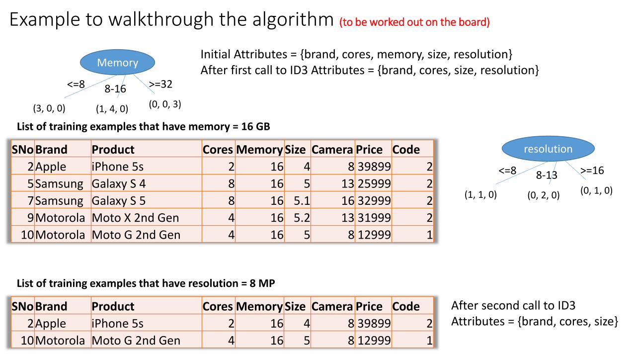
Example to walkthrough the algorithm (to be worked out on the board)

Memory

<=8 8-16 >=32

(3, 0, 0) (1, 4, 0) (0, 0, 3)

Initial Attributes = {brand, cores, memory, size, resolution}After first call to ID3 Attributes = {brand, cores, size, resolution}

SNoBrand Product Cores Memory Size Camera Price Code

2Apple iPhone 5s 2 16 4 8 39899 2

5Samsung Galaxy S 4 8 16 5 13 25999 2

7Samsung Galaxy S 5 8 16 5.1 16 32999 2

9Motorola Moto X 2nd Gen 4 16 5.2 13 31999 2

10Motorola Moto G 2nd Gen 4 16 5 8 12999 1

List of training examples that have memory = 16 GB

resolution

<=8 8-13 >=16

(1, 1, 0) (0, 2, 0) (0, 1, 0)

SNoBrand Product Cores Memory Size Camera Price Code

2Apple iPhone 5s 2 16 4 8 39899 2

10Motorola Moto G 2nd Gen 4 16 5 8 12999 1

List of training examples that have resolution = 8 MP

After second call to ID3 Attributes = {brand, cores, size}

CART For our example

Memory

<=8 8-16 >=32

resolution

<=8 8-13 >=16

Brand

Motorola Apple

1 3

21

1 2

• The interpretability of the trees enable us to easily glean the knowledge encoded in the dataset.

• Some other machine learning techniques such as deep neural networks with many layers of parameters are hard to interpret. Though it is possible to visualize the parameters from the layers, interpreting the trees is easier and intuitive.

• The attributes that discriminate the dataset provide several valuable insights, for example:- Which attribute make a huge difference to the price?- At what values of these attributes does the price tends to

get exponentially steeper?- Looking at the brands and the product features, what can

we infer on their business strategy? Where do they try to differentiate themselves?

Intuition behind entropy (Ref: C Bishop)

• Consider a discrete random variable x. How much information we receive when we observe a specific value of x?

• The amount of information can be viewed as the degree of surprise on learning the value of x. That is a highly improbable information provides more information compared to a more likely event. When an event is certain to happen we receive zero information.

• Hence the information h(x) is a monotonic function of probability p(x)

• If there are 2 independent events, the information that we receive on both the events is the sum of information we gained from each of them separately. Hence: h(x, y) = h(x) + h(y)

• Two unrelated events will be statistically independent if: p(x, y) = p(x) p(y)

• From the above 2 relationships we deduce that h(x) should be related to log p(x). Specifically: h(x) = - log2p(x).

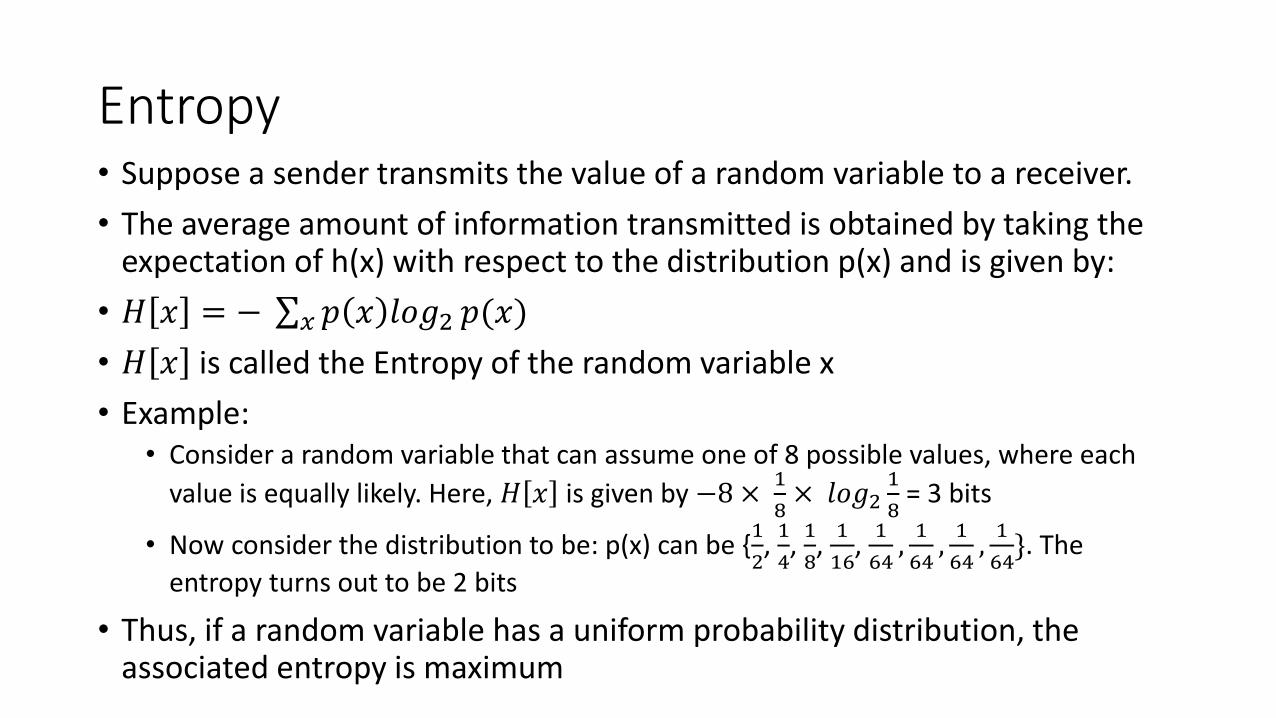
Entropy• Suppose a sender transmits the value of a random variable to a receiver.

• The average amount of information transmitted is obtained by taking the expectation of h(x) with respect to the distribution p(x) and is given by:

• 𝐻 𝑥 = − 𝑥 𝑝 𝑥 𝑙𝑜𝑔2 𝑝(𝑥)

• 𝐻 𝑥 is called the Entropy of the random variable x

• Example:• Consider a random variable that can assume one of 8 possible values, where each

value is equally likely. Here, 𝐻 𝑥 is given by −8 ×1

8× 𝑙𝑜𝑔2

1

8= 3 bits

• Now consider the distribution to be: p(x) can be {1

2, 1

4, 1

8, 1

16, 1

64,1

64,1

64,1

64}. The

entropy turns out to be 2 bits

• Thus, if a random variable has a uniform probability distribution, the associated entropy is maximum

Sample Entropy

• Entropy is maximum when the probability of positive and negative cases are equal

Conditional Entropy Ref: T Mitchell

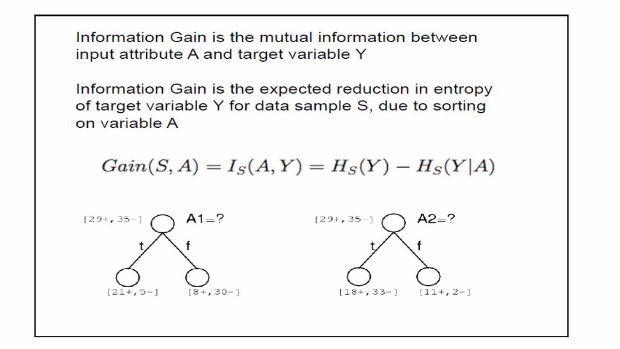
Information Gain

• Exercise: Work it out for our mobile price classification example

𝐺𝑎𝑖𝑛 𝑆, 𝐴 ≡ 𝐸𝑛𝑡𝑟𝑜𝑝𝑦 𝑆 −

𝑣 ∈𝑉𝑎𝑙𝑢𝑒𝑠(𝐴)

𝑆𝑣|𝑆|𝐸𝑛𝑡𝑟𝑜𝑝𝑦(𝑆𝑣)

CART Models – Pros and Cons• Easy to explain and interpret: We can derive if then else rules from CART trees, we can visualize the trees

• Handles discrete and continuous variables

• Robust to outliers

• Can handle missing inputs

• Can scale to large datasets

• The cost of using the tree (i.e., predicting data) is logarithmic in the number of data points used to train the tree.

• Can perform automatic variable selection

• Uses a white box model. If a given situation is observable in a model, the explanation for the condition is easily explained by boolean logic. By contrast, in a black box model (e.g., in an artificial neural network), results may be more difficult to interpret.

• Relatively, accuracy of prediction may not be the best – possibly due to greedy algorithm

• Sensitive to data - overfitting

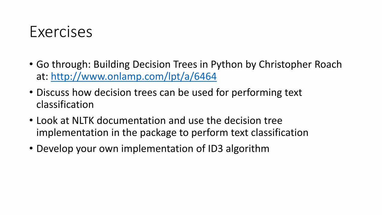
Exercises

• Go through: Building Decision Trees in Python by Christopher Roach at: http://www.onlamp.com/lpt/a/6464

• Discuss how decision trees can be used for performing text classification

• Look at NLTK documentation and use the decision tree implementation in the package to perform text classification

• Develop your own implementation of ID3 algorithm