machine learning methods for histopathological image analysis
TRANSCRIPT

Machine learning methods for histopathological
image analysis
Daisuke Komura1, Shumpei Ishikawa1*
* Corresponding author
1Department of Genomic Pathology, Medical Research Institute, Tokyo Medical and Dental University, Tokyo,
Japan

Abstract
Abundant accumulation of digital histopathological images has led to the increased demand for their analysis,
such as computer-aided diagnosis using machine learning techniques. However, digital pathological images
and related tasks have some issues to be considered. In this mini-review, we introduce the application of digital
pathological image analysis using machine learning algorithms, address some problems specific to such
analysis, and propose possible solutions.
Keywords: histopathology; deep learning; machine learning; whole slide images; computer assisted diagnosis;
digital image analysis
1. Introduction
Pathology diagnosis has been performed by a human pathologist observing the stained specimen on the slide
glass using a microscope. In recent years, attempts have been made to capture the entire slide with a scanner
and save it as a digital image (Whole slide image, WSI) [1]. As a large number of WSI are being accumulated,
attempts have been made to analyze WSIs using digital image analysis based on machine learning algorithms
to assist tasks including diagnosis.
Digital pathological image analysis often uses general image recognition technology (e.g. facial recognition)
as a basis. However, since digital pathological images and tasks have some unique characteristics, special
processing techniques are often required. In this review, we describe the application of digital pathological
image analysis using machine learning algorithms, and its problems specific to digital pathological image
analysis and the possible solutions. Several reviews that have been published recently discuss
histopathological image analysis including its history and details of general machine learning algorithms [2–
7]; in this review, we provide more pathology-oriented point of view.
Since the overwhelming victory of the team using deep learning at ImageNet Large Scale Visual Recognition
Competition (ILSVRC) 2012 [8], most of the image recognition techniques have been replaced by deep
learning. This is also true for pathological image analysis [9–11]. Therefore, even though many techniques
introduced in this review are related to deep learning, most of them are also applicable for other machine
learning algorithms.
2. Machine learning methods
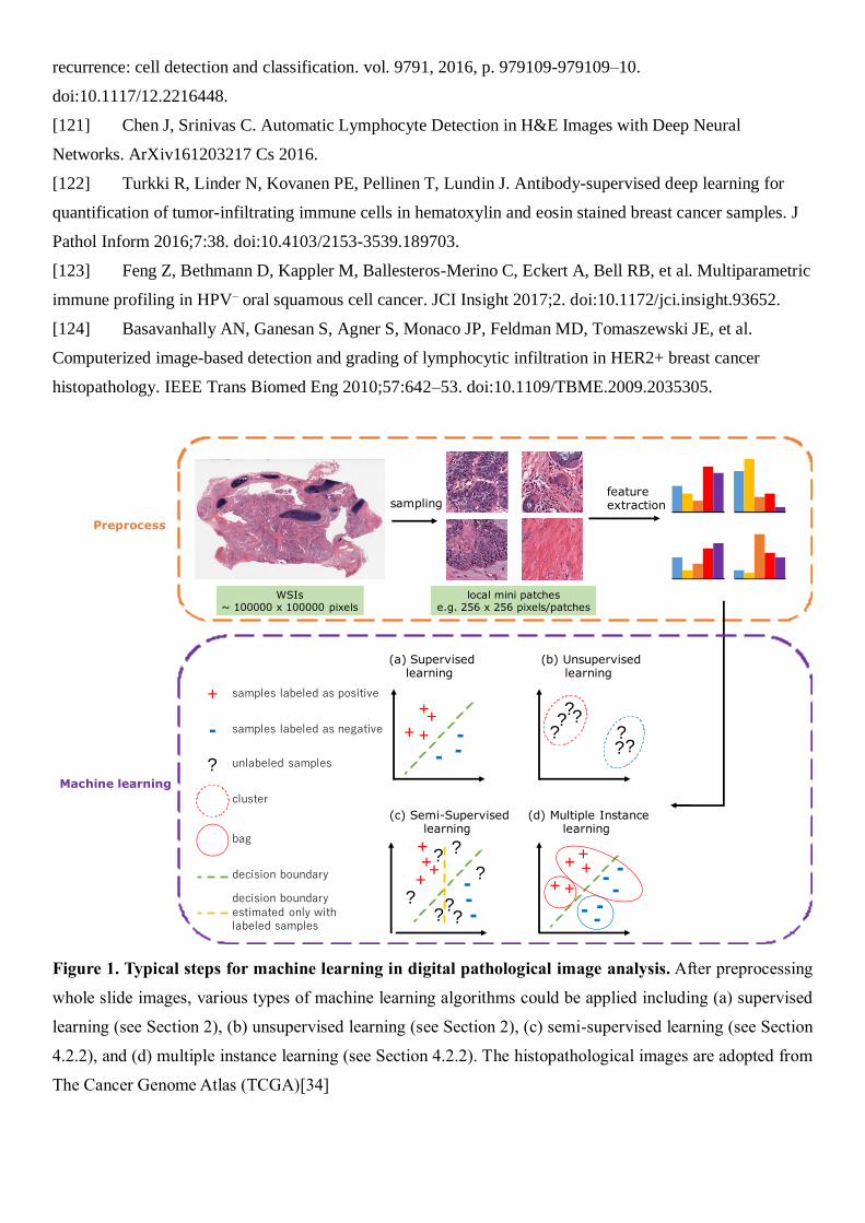
Figure 1 shows typical steps for histopathological image analysis using machine learning. Prior to applying
machine learning algorithms, some pre-processing should be performed. For example, when cancer regions
are detected in WSI, local mini patches around 256 × 256 are sampled from large WSI. Then feature extraction
and classification between cancer and non-cancer are performed in each local patch. The goal of feature
extraction is to extract useful information for machine learning tasks. Various local features such as gray level
co-occurrence Matrix (GLCM) and local binary pattern (LBP) have been used for histopathological image
analysis, but deep learning algorithms such as convolutional neural network [9,10,12–14] starts the analysis

from feature extraction. Features and classifiers are simultaneously optimized in deep learning and features
learned in deep learning often outperforms other traditional features in histopathological image analysis.
Machine learning techniques often used in digital pathology image analysis are divided into supervised
learning and unsupervised learning. The goal of supervised learning is to infer a function that can map the
input images to their appropriate labels (e.g. cancer) well using training data. Labels are associated with a
WSI or an object in WSIs. The algorithms for supervised learning include support vector machines, random
forest and convolutional neural networks. On the other hand, the goal of unsupervised learning is to infer a
function that can describe hidden structures from unlabeled images. The tasks include clustering, anomaly
detection and dimensionality reduction. The algorithms for unsupervised learning include k-means,
autoencoders and principal component analysis. There are derivatives from these two learning such as semi-
supervised learning and multiple instance learning, which are described in Section 4.2.2.
3. Machine learning application in digital pathology
3.1. Computer-assisted diagnosis
The most actively researched task in digital pathological image analysis is computer-assisted diagnosis (CAD),
which is the basic task of the pathologist. Diagnostic process contains the task to map a WSI or multiple WSIs
to one of the disease categories, meaning that it is essentially a supervised learning task. Since the errors made
by a machine learning system reportedly differ from those made by a human pathologist [15], classification
accuracy could be improved using CAD system. CAD may also lead to the reduce variability in interpretations
and prevent overlooking by investigating all pixels within WSIs.
Other diagnosis-related tasks include detection or segmentation of Region of Interest (ROI) such as tumor
region in WSI [16,17], scoring of immunostaining [11,18], cancer staging [15,19], mitosis detection [20,21],
gland segmentation [22–24], and detection and quantification of vascular invasion [25].
3.2. Content Based Image Retrieval
Content Based Image Retrieval (CBIR) retrieves similar images to a query image. In digital pathology, CBIR
systems are useful in many situations, particularly in diagnosis, education, and research [26–31]. For example,
CBIR systems can be used for educational purposes by students and beginner pathologists to retrieve relevant
cases or histopathological images of tissues. In addition, such systems are also helpful to professional
pathologists, particularly when diagnosing of rare cases.
Since CBIR does not necessarily require label information, unsupervised learning can be used [30]. When
label information is available, supervised learning approaches could learn better similarity measure than
unsupervised learning approaches [28,29] since the similarity between histopathological images may differ
by definition. However, preparing sufficient number of labeled data can be a serious problem as will be
described later.
In CBIR, not only accuracy but also high-speed search of similar images from numerous images are required.

Therefore, various techniques for dimensionality reduction of image features such as principal component
analysis and compact bilinear pooling [32], and fast approximate nearest neighbor search such as kd-tree
and hashing [33] are utilized for high speed search.
3.3. Discovering new clinicopathological relationships
Historically, many important discoveries concerning diseases such as tumor and infectious diseases have
been made by pathologists and researchers who have carefully and closely observed pathological specimens.
For example, H. pylori was discovered by a pathologist who was examining the gastric mucosa of patients
with gastritis [34]. Attempts have also been made to correlate the morphological features of cancers with their
clinical behavior. For example, tumor grading is important in planning treatment and determining a patient’s
prognosis for certain types of cancer, such as soft tissue sarcoma, primary brain tumors, and breast and prostate
cancer.
Meanwhile, thanks to the progress in digitization of medical information and advance in genome analysis
technology in recent years, large amount of digital information such as genome information, digital
pathological images, MRI and CT images has become available [35]. By analyzing the relationship between
these data, new clinicopathological relationships, for example, the relationship between the morphological
characteristic and the somatic mutation of the cancer, can be found [35,36]. However, since the amount of
data is enormous, it is not realistic for pathologists and researchers to analyze all the relationships manually
by looking at the specimens. This is where the machine learning technology comes in. For example, Beck et
al. extracted texture information from pathological images of breast cancer and analyzed with L1 - regularized
logistic regression, and indicated that the histology of stroma correlates with prognosis in breast cancer [37].
Other researches include prognosis predictions from histopathological image of cancer [38], prediction of
somatic mutation [13], and discovery of new gene variants related to autoimmune thyroiditis based on image
QTL [39].
4. Problems specific to histopathological image analysis
In this section, we describe unique characteristics of pathological image analysis and computational methods
to treat them. Table 1 presents an overview of papers dealing with the problems and the solutions.
Table 1. Overview of papers dealing with problems and solutions for histopathological image analysis
Solution reference
Very large image size
Case level classification summarizing
patch or object level classification
Markov Random Field [17], Bag of Words of local
structure [18] and random forest [14,40,41]
Insufficient labeled images
GUI tools Web server [42,43]

Tracking pathologists' behavior Eye tracking [44], mouse tracking [45] and viewport
tracking [46]
Active learning Uncertainly sampling [43], Query-by-Committee [47],
variance reduction [48] and hypothesis space reduction
[49]
Multiple instance learning Boosting-based [50,51], deep weak supervision [52]
and structured support vector machines (SVM) [53]
Semi-supervised learning Manifold learning [30] and SVM [54]
Transfer learning Feature extraction [55], fine-tuning [16,56,57]
Different levels of magnification result in different levels of information
Multiscale analysis CNN [58], dictionary learning [59] and texture features
[60]
WSI as orderless texture-like image
Texture features Traditional textures [61–64] and CNN-based textures
[65]
Color variation and artifacts
Removal of color variation effect Color normalization [66–69] and color augmentation
70,71]
Artifact detection Blur [72,73] and tissue-folds [74,75]
4.1. Very large image size
When images such as dogs or houses are classified using deep learning, small sized image such as 256 × 256
pixels is often used as an input. Images with large size often need to be resized into smaller size which is
enough for sufficient distinction, as increase in the size of the input image results in the increase in the
parameter to be estimated, the required computational power, and memory. In contrast, WSI contains many
cells and the image could consist of as many as tens of billions of pixels, which is usually hard to analyzed as
is. However, resizing the entire image to a smaller size such as 256 × 256 would lead to the loss of information
at cellular level, resulting in marked decrease of the identification accuracy. Therefore, the entire WSI is
commonly divided into partial regions of about 256 × 256 pixels (“patches”), and each patch is analyzed
independently, such as detection of ROIs. Thanks to the advances in computational power and memory, patch
size is increasing (e.g. 960 × 960), which is expected to contribute to better accuracy. There is still a room for
improvement in the method of integrating the result from each patch. For example, as the entire WSI could
contain hundreds of thousands of patches, false positives are highly likely to appear even if individual patches
are accurately classified. One possible solution for this is regional averaging of each decision, such that the

regions is classified as ROI only when the ROI extends over multiple patches. However, this approach may
suffer from false negatives, resulting in missing small ROIs such as isolated tumor cells [41].
In some applications such as IHC scoring, staging of lymph node metastasis of specimens or patients, and
staging of prostate cancer diagnosed by Glisson score of multiple regions within one slide, more sophisticated
algorithms to integrate patch-level or object-level decisions are required [14,17,18,40,41,76]. For example,
for pN-staging of metastatic breast cancer, which was one of the tasks in Camelyon 17, multiple participating
teams including us applied random forest classifiers of pixel or patch-level probabilities estimated by deep
learning using various features such as estimated tumor size [41].
4.2. Insufficient labeled images
Probably the biggest problem in pathological image analysis using machine learning is that only a small
number of training data is available. A key to the success of deep learning in general image recognition task
is that training data is extremely abundant. Although label information at patch-level or pixel-level (e.g.
inside/outside boundary of cancerous regions) is required in most tasks in digital pathology such as diagnosis,
most labels of WSIs are at case-level (e.g. diagnosis) at most. Label information in general image analysis can
be easily retrieved from the internet and it is also possible to use crowdsource labeling because anyone can
identify objects and perform labeled work. However, only pathologists can label the pathological image
accurately, and labeling at the regional level in a huge WSIs requires a lot of labor.
It is possible to reuse public ready-to-analyze data as training data in machine learning, such as ImageNet
[77] in natural images and International Skin Imaging Collaboration [78] in macroscopic diagnosis of skin. In
the field of digital pathology, there are some public datasets that contain hand-annotated histopathological
images as summarized in Table 1 and Table 2. They could be useful if the purpose of the analysis, slide
condition (e.g. stain), and image condition (e.g. magnification level and image resolution) are similar.
However, because each of these datasets focuses on specific disease or cell types, many tasks are not covered
by these datasets. There are also several large-scale histopathological image databases that contain high-
resolution WSIs: The Cancer Genome Atlas (TCGA) [79] contains over 10000 WSIs from various cancer
types, and Genotype-Tissue Expression (GTEx) [80,81]contains over 20000 WSIs from various tissues. These
databases may serve as potential training data for various tasks. Furthermore, both TCGA and GTEx also
provide genomic profiles, which could be used to investigate relationships between genotype and morphology.
The problem is that the WSIs in these repositories contain labels at the case-level, and in order to be able to
use them for training data, some preprocessing or specialized machine learning algorithm for treating case-
level labels is required.
Many researches have attempted to solve the problem. Most of the approaches fall into one of the following
categories: 1) efficient increase of label data, 2) utilization of weak label or unlabeled information, or 3)
utilization of models/parameters for other tasks.
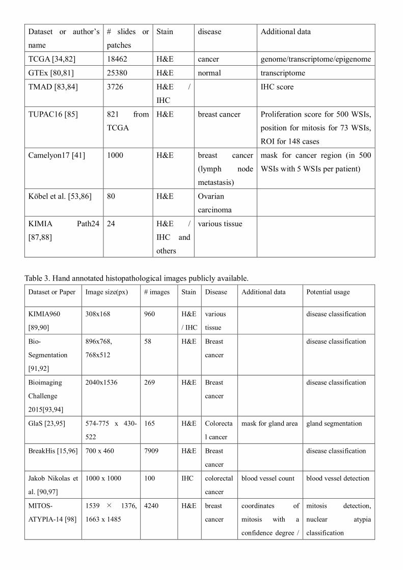
Table 2. downloadable WSI database.
Dataset or author’s
name
# slides or
patches
Stain disease Additional data
TCGA [34,82] 18462 H&E cancer genome/transcriptome/epigenome
GTEx [80,81] 25380 H&E normal transcriptome
TMAD [83,84] 3726 H&E /
IHC
IHC score
TUPAC16 [85] 821 from
TCGA
H&E breast cancer Proliferation score for 500 WSIs,
position for mitosis for 73 WSIs,
ROI for 148 cases
Camelyon17 [41] 1000 H&E breast cancer
(lymph node
metastasis)
mask for cancer region (in 500
WSIs with 5 WSIs per patient)
Köbel et al. [53,86] 80 H&E Ovarian
carcinoma
KIMIA Path24
[87,88]
24 H&E /
IHC and
others
various tissue
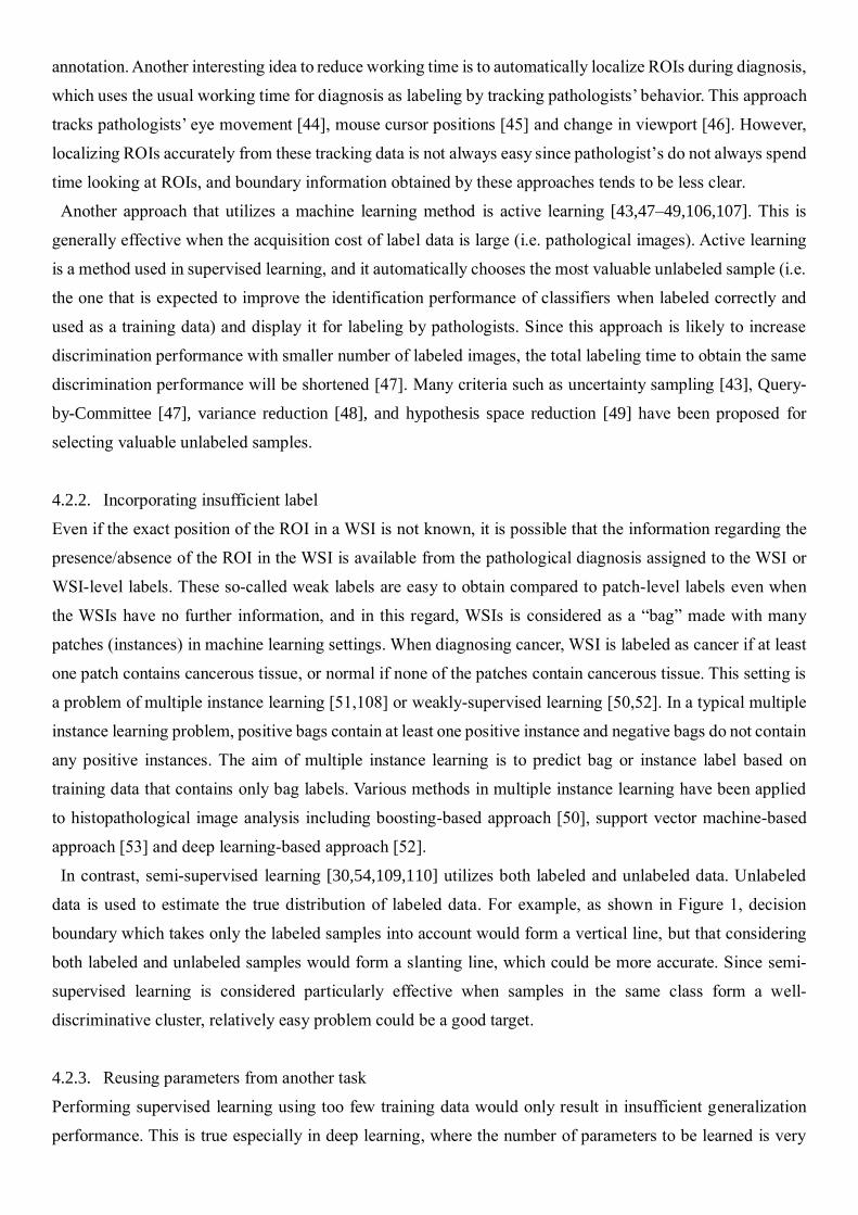
Table 3. Hand annotated histopathological images publicly available.
Dataset or Paper Image size(px) # images Stain Disease Additional data Potential usage
KIMIA960
[89,90]
308x168 960 H&E
/ IHC
various
tissue
disease classification
Bio-
Segmentation
[91,92]
896x768,
768x512
58 H&E Breast
cancer
disease classification
Bioimaging
Challenge
2015[93,94]
2040x1536 269 H&E Breast
cancer
disease classification
GlaS [23,95] 574-775 x 430-
522
165 H&E Colorecta
l cancer
mask for gland area gland segmentation
BreakHis [15,96] 700 x 460 7909 H&E Breast
cancer
disease classification
Jakob Nikolas et
al. [90,97]
1000 x 1000 100 IHC colorectal
cancer
blood vessel count blood vessel detection
MITOS-
ATYPIA-14 [98]
1539 × 1376,
1663 x 1485
4240 H&E breast
cancer
coordinates of
mitosis with a
confidence degree /
mitosis detection,
nuclear atypia
classification

six criteria to
evaluate nuclear
atypia
Kumar et al
[99,100]
1000 x 1000 30 H&E various
cancer
coordinates of
annotated nuclear
boundaries
nuclear segmentation
MITOS 2012
[20,101]
2084 x 2084,
2252 x 2250
100 H&E breast
cancer
coordinates of
mitosis
mitosis detection
Janowczyk et al.
[102,103]
1388 x 1040 374 H&E lymphom
a
none disease classification
Janowczyk et al.
[102,103]
2000 x 2000 311 H&E breast
cancer
coordinates of
mitosis
mitosis detection
Janowczyk et al.
[102,103]
100 x 100 100 H&E breast
cancer
coordinates of
lymphocyte
lymphocyte detection
Janowczyk et al.
[102,103]
1000 x 1000 42 H&E breast
cancer
mask for epithelium epithelium
segmentation
Janowczyk et al.
[102,103]
2000 x 2000 143 H&E breast
cancer
mask for nuclei nuclear segmentation
Janowczyk et al.
[102,103]
775 x 522 85 H&E colorectal
cancer
mask for gland area gland segmentation
Janowczyk et al.
[102,103]
50 x 50 277524 H&E breast
cancer
none tumor detection
Gertych et al[22] 1200 x 1200 210 H&E prostate
cancer
mask for gland area gland segmentation
Ma et al[104] 1040x1392 81 IHC breast
cancer
TIL analysis
Linder et al.
[64,105]
93-2372 x 94-
2373
1377 IHC colorectal
cancer
mask for epithelium
and stroma
segmentation of
epithelium and stroma
Xu et al. [55] various size 717 H&E colon
cancer
Xu et al. [55] 1280 x 800 300 H&E colon
cancer
mask for colon
cancer
segmentation
4.2.1. Efficient labeling
One way to increase training data is to reduce the working time of pathologists to specify ROIs in the WSI.
Easy-to-use GUI tools helps pathologists efficiently label more samples in shorter periods of time [42,43]. For
example, Cytomine [42] not only allows pathologists to surround ROIs in WSIs with ellipses, rectangles,
polygons or freehand drawings, but also applies content-based image retrieval algorithms to speed up
annotation. Another interesting idea to reduce working time is to automatically localize ROIs during diagnosis,
which uses the usual working time for diagnosis as labeling by tracking pathologists’ behavior. This approach
tracks pathologists’ eye movement [44], mouse cursor positions [45] and change in viewport [46]. However,
localizing ROIs accurately from these tracking data is not always easy since pathologist’s do not always spend
time looking at ROIs, and boundary information obtained by these approaches tends to be less clear.
Another approach that utilizes a machine learning method is active learning [43,47–49,106,107]. This is
generally effective when the acquisition cost of label data is large (i.e. pathological images). Active learning
is a method used in supervised learning, and it automatically chooses the most valuable unlabeled sample (i.e.
the one that is expected to improve the identification performance of classifiers when labeled correctly and
used as a training data) and display it for labeling by pathologists. Since this approach is likely to increase
discrimination performance with smaller number of labeled images, the total labeling time to obtain the same
discrimination performance will be shortened [47]. Many criteria such as uncertainty sampling [43], Query-
by-Committee [47], variance reduction [48], and hypothesis space reduction [49] have been proposed for
selecting valuable unlabeled samples.
4.2.2. Incorporating insufficient label
Even if the exact position of the ROI in a WSI is not known, it is possible that the information regarding the
presence/absence of the ROI in the WSI is available from the pathological diagnosis assigned to the WSI or
WSI-level labels. These so-called weak labels are easy to obtain compared to patch-level labels even when
the WSIs have no further information, and in this regard, WSIs is considered as a “bag” made with many
patches (instances) in machine learning settings. When diagnosing cancer, WSI is labeled as cancer if at least
one patch contains cancerous tissue, or normal if none of the patches contain cancerous tissue. This setting is
a problem of multiple instance learning [51,108] or weakly-supervised learning [50,52]. In a typical multiple
instance learning problem, positive bags contain at least one positive instance and negative bags do not contain
any positive instances. The aim of multiple instance learning is to predict bag or instance label based on
training data that contains only bag labels. Various methods in multiple instance learning have been applied
to histopathological image analysis including boosting-based approach [50], support vector machine-based
approach [53] and deep learning-based approach [52].
In contrast, semi-supervised learning [30,54,109,110] utilizes both labeled and unlabeled data. Unlabeled
data is used to estimate the true distribution of labeled data. For example, as shown in Figure 1, decision
boundary which takes only the labeled samples into account would form a vertical line, but that considering
both labeled and unlabeled samples would form a slanting line, which could be more accurate. Since semi-
supervised learning is considered particularly effective when samples in the same class form a well-
discriminative cluster, relatively easy problem could be a good target.
4.2.3. Reusing parameters from another task
Performing supervised learning using too few training data would only result in insufficient generalization
performance. This is true especially in deep learning, where the number of parameters to be learned is very
large. In such a case, instead of learning the entire model from scratch, learning often starts by using (a part
of) parameters of a pre-trained model optimized in another similar task. Such a learning method is called
transfer learning. In CNN, layers before the last (typically three) fully-connected layers are regarded as feature
extractors. The fully-connected layers are often replaced by a new network suitable for the target task. The
parameters in earlier layers can be used as is [55], or as initial parameters and then the network is learned
partially or fully from the training data of the target task [16,56,57] (so-called fine-tuning). In pathological
images, no network learned from tasks using other pathological images are available, and thus networks
learned using ImageNet, which is a database containing vast number of general images, are often used [16,55–
57]. For example, Xu et al., performed classification and segmentation tasks on brain and colon pathological
images using features extracted from CNN trained on ImageNet, and achieved state-of-the-art performance
[55]. Although the pathological image itself looks very different to the general images (e.g. cats and dogs),
they share common basic image structures such as lines and arcs. Since earlier layers in deep learning capture
these basic image structures, such pre-trained models using general images work well in histopathological
image analysis. Nevertheless, if models pre-trained on sufficient number of diverse tissue pathology images
are available, they may outperform the ImageNet pre-trained models.
4.3. Different levels of magnification result in different levels of information
Tissues are usually composed of cells, and different tissues show distinct cellular features. Information
regarding cell shape is well captured in high-power field microscopic images, but structural information such
as a glandular structure made of many cells are better captured in a lower-power field (Figure 2). Because
cancerous tissues have both cellular and structural atypia, images taken at multiple magnifications would each
contain important information. Pathologists diagnose diseases by acquiring different kinds of information
from the cellular level to the tissue level by changing magnifications of a microscope. Even in machine
learning, researches utilizing images at different magnifications exist [58–60]. As mentioned above, it is
difficult to handle the images at its original resolution directly, images are often resized to correspond to
various magnifications and used as input for analysis. Regarding diagnosis, the most informative
magnification is still controversial [14,40,111], but improvement in accuracy is sometimes achieved by
inputting both high and low magnification images simultaneously, probably depending on the types of diseases
and tissues, and machine learning algorithms.
4.4. WSI as orderless texture-like image
Pathological image is different from cats and dogs in nature, in a sense that it shows repetitive pattern of
minimum components (usually cells). Therefore, it is rather closer to texture than object. CNN acquires shift
invariance to a certain extent by pooling operations. In addition, even normal CNN can learn texture-like
structure by data augmentation by shifting the tissue image with a small stride. Meanwhile, there has been
methods which utilize texture structure more intensively, such as gray level co-occurrence matrix [112], local
binary pattern [113], Gabor filter bank, and recently developed deep texture representations using a CNN
[65,114]. Deep texture representations are computed using a correlation matrix of feature maps in a CNN layer.

Converting the CNN features to texture representations would lead to the acquisition of invariance regarding
cell position, while utilizing good representations learned by CNN. Another advantage of deep texture
representation is that there are no constraints on the size of input image, which is very suitable for large image
size of WSI. The boundary between texture and non-texture is unclear, but a single cell or a single structure is
obviously not a texture. Better approach would thus depend on the object to be analyzed.
4.5. Color variation and artifacts
WSIs are created through multiple processes: pathology specimens are sliced and placed on a slide glass,
stained with hematoxylin and eosin, and then scanned. At each step undesirable effects, which are unrelated
to the underlying biological factors, could be introduced. For example, when tissue slices are being placed
onto the slides, they may be bent and wrinkled; dust may contaminate the slides during scanning; blur
attributable to different thickness of tissue sections may occur (Figure 3); and sometimes tissue regions are
marked by color markers. Since these artifacts could adversely affect the interpretation, specific algorithms to
detect artifacts such as blur [72] and tissue-folds [74] have been proposed. Such algorithms may be used for
preprocessing WSIs.
Another serious artifact is color variation as shown in Figure 4. The sources of variation include different
lots or manufacturers of staining reagents, thickness of tissue sections, staining conditions and scanner models.
Learning without considering the color variation could worsen the performance of machine learning algorithm.
If sufficient data on every stained tissue acquired by every scanner can be incorporated, the influence of color
variation on classification accuracy may become negligible; however, that seems very unlikely at the moment.
To address this issue, various methods have been proposed so far including conversion to gray scale, color
normalization [66–69], and color augmentation [70,71]. Conversion to grayscale is the easiest way, but it
ignores the important information regarding the color representation used routinely by pathologists. In contrast,
color normalization tries to adjust the color values of an image on a pixel-by-pixel basis so that the color
distribution of the source image matches to that of a reference image. However, as the components and
composition ratios of cells or tissues in target and reference images differ in general, preprocessing such as
nuclear detection using a dedicated algorithm to adjust the component is often required. For this reason, color
normalization seems to be suitable when WSIs analyzed in the tasks contain, at least partially, similar
compositions of cells or tissues.
On the other hand, color augmentation is a kind of data augmentation performed by applying random hue,
saturation, brightness, and contrast. The advantage of color augmentation lies in the easy implementation
regardless of the object being analyzed. Color augmentation seems to be suitable for WSIs with smaller color
variation, since excessive color change in color augmentation could lead to the loss of color information in
the final classifier. As color normalization and color augmentation could be complementary, combination of
both approaches may be better.
5. Summary and Outlook
Digital histopathological image recognition is a very suitable problem for machine learning since the images

themselves contain information sufficient for diagnosis. In this review, we brought up problems in digital
histopathological image analysis using machine learning. Due to great efforts made so far, these problems are
becoming tractable, but there is still room for improvement. Most of these problems are likely to be solved
once a large number of well-annotated WSIs become available. Gathering WSIs from various institutes to
collaboratively annotate them with the same criteria and making these data public will be sufficient to boost
the development of more sophisticated digital histopathological image analysis.
Finally, we suggest some potential future research topics that have not been well studied so far.
Discovery of novel objects
In actual diagnostic situations, unexpected objects such as aberrant organization, rare tumor (thus not included
in training data) and foreign bodies could exist. However, discrimination model including Convolutional
Neural Networks forcibly categorizes such objects into one of the pre-defined categories. To solve the problem,
outlier detection algorithms, such as one-class kernel principal component analysis[115], have been applied
to the digital pathological images but only a few researches have addressed the problem so far. More recently,
some deep learning-based methods utilizing reconstruction error [116] have been proposed for outlier
detection in other domains, but they are not yet applied in the histopathological image analysis.
Interpretable deep learning model
Deep learning is often criticized because its decision-making process is not understandable to humans and
therefore often described as being a black box. Although decision-making process of human is not a complete
white box either, people want to know the decision process or decision basis. This could lead to a new
discovery in the pathology field. Although this problem has not been completely solved so far, some research
has attempted to provide solutions, such as joint learning of pathological images and its diagnostic reports
integrated with attention mechanism[117]. In other domains, decision basis can be inferredindirectly
represented by visualizing the response of a deep neural network[117,118], or presenting the most helpful
training image using influence functions[119].
Intraoperative diagnosis
Pathological diagnosis during surgery influences intraoperative decision making, and thus could be another
important application in histopathological image analysis. As diagnostic time in intraoperative diagnosis is
very limited, rapid classification while keeping accuracy is of importance. Due to the time constraint, rapid
frozen section is used instead of Formalin-fixed paraffin-embedded (FFPE) section which takes longer time
to prepare. Therefore, for this purpose training of classifiers should be performed using frozen section slides.
Few research has analyzed frozen sections [120] so far partly because the number of WSIs suitable for the
analysis is not sufficient, and task is more challenging compared to FFPE slides.
Tumor infiltrating immune cell analysis
Because of the success of tumor immunotherapy, especially immune-checkpoint blockade therapies including

anti-PD-1 and anti-CTLA-4 antibodies, immune cells in tumor microenvironment have gained substantial
attention in recent years. Therefore, quantitative analysis of tumor infiltrating immune cells in slides using
machine learning techniques will be one of the emerging themes in digital histopathological image analysis.
Tasks related to this analysis include detection of immune cells from H&E stained image[121,122] and
detection of more specific type of immune cells using immunohistochemistry[104]. Additionally, the pattern
of immune cell infiltration and proximity of each immune cells are reportedly related to cancer prognosis[123],
analysis of spatial relationships between tumor cells and immune cells, and the relationships between these
data and prognosis or response to immunotherapy using specialized algorithms such as graph-based
algorithms [63,124] will also be of great importance.
Acknowledgement
This study was supported by JSPS Grant-in-Aid for Scientific Research (A), No. 25710020 (SI).
[1] Pantanowitz L. Digital images and the future of digital pathology. J Pathol Inform 2010;1.
doi:10.4103/2153-3539.68332.
[2] Shen D, Wu G, Suk H-I. Deep Learning in Medical Image Analysis. Annu Rev Biomed Eng
2017;19:221–48. doi:10.1146/annurev-bioeng-071516-044442.
[3] Bhargava R, Madabhushi A. Emerging Themes in Image Informatics and Molecular Analysis for
Digital Pathology. Annu Rev Biomed Eng 2016;18:387–412. doi:10.1146/annurev-bioeng-112415-114722.
[4] Madabhushi A. Digital pathology image analysis: opportunities and challenges. Imaging Med
2009;1:7.
[5] Gurcan MN, Boucheron L, Can A, Madabhushi A, Rajpoot N, Yener B. Histopathological Image
Analysis: A Review. IEEE Rev Biomed Eng 2009;2:147–71. doi:10.1109/RBME.2009.2034865.
[6] Litjens G, Kooi T, Bejnordi BE, Setio AAA, Ciompi F, Ghafoorian M, et al. A survey on deep
learning in medical image analysis. Med Image Anal 2017;42:60–88. doi:10.1016/j.media.2017.07.005.
[7] Xing F, Yang L. Robust Nucleus/Cell Detection and Segmentation in Digital Pathology and
Microscopy Images: A Comprehensive Review. IEEE Rev Biomed Eng 2016;9:234–63.
doi:10.1109/RBME.2016.2515127.
[8] Krizhevsky A, Sutskever I, Hinton GE. ImageNet Classification with Deep Convolutional Neural
Networks. In: Pereira F, Burges CJC, Bottou L, Weinberger KQ, editors. Adv. Neural Inf. Process. Syst. 25,
Curran Associates, Inc.; 2012, p. 1097–1105.
[9] Hou L, Samaras D, Kurc TM, Gao Y, Davis JE, Saltz JH. Patch-based Convolutional Neural
Network for Whole Slide Tissue Image Classification. ArXiv150407947 Cs 2015.
[10] Xu J, Luo X, Wang G, Gilmore H, Madabhushi A. A Deep Convolutional Neural Network for
segmenting and classifying epithelial and stromal regions in histopathological images. Neurocomputing
2016;191:214–23. doi:10.1016/j.neucom.2016.01.034.
[11] Sheikhzadeh F, Guillaud M, Ward RK. Automatic labeling of molecular biomarkers of whole
slide immunohistochemistry images using fully convolutional networks. ArXiv161209420 Cs Q-Bio 2016.
[12] Litjens G, Sánchez CI, Timofeeva N, Hermsen M, Nagtegaal I, Kovacs I, et al. Deep learning as a
tool for increased accuracy and efficiency of histopathological diagnosis. Sci Rep 2016;6:26286.
doi:10.1038/srep26286.
[13] Schaumberg AJ, Rubin MA, Fuchs TJ. H&E-stained Whole Slide Image Deep Learning
Predicts SPOP Mutation State in Prostate Cancer. BioRxiv 2017:064279. doi:10.1101/064279.
[14] Wang D, Khosla A, Gargeya R, Irshad H, Beck AH. Deep Learning for Identifying Metastatic
Breast Cancer. ArXiv160605718 Cs Q-Bio 2016.
[15] Spanhol FA, Oliveira LS, Petitjean C, Heutte L. Breast cancer histopathological image
classification using Convolutional Neural Networks. 2016 Int. Jt. Conf. Neural Netw. IJCNN, 2016, p.
2560–7. doi:10.1109/IJCNN.2016.7727519.
[16] Kieffer B, Babaie M, Kalra S, Tizhoosh HR. Convolutional Neural Networks for Histopathology
Image Classification: Training vs. Using Pre-Trained Networks. ArXiv171005726 Cs 2017.
[17] Mungle T, Tewary S, Das DK, Arun I, Basak B, Agarwal S, et al. MRF-ANN: a machine learning
approach for automated ER scoring of breast cancer immunohistochemical images. J Microsc
2017;267:117–29. doi:10.1111/jmi.12552.
[18] Wang D, Foran DJ, Ren J, Zhong H, Kim IY, Qi X. Exploring automatic prostate histopathology
image gleason grading via local structure modeling. 2015 37th Annu. Int. Conf. IEEE Eng. Med. Biol. Soc.
EMBC, 2015, p. 2649–52. doi:10.1109/EMBC.2015.7318936.
[19] Shah M, Rubadue C, Suster D, Wang D. Deep Learning Assessment of Tumor Proliferation in
Breast Cancer Histological Images. ArXiv161003467 Cs 2016.
[20] Roux L, Racoceanu D, Loménie N, Kulikova M, Irshad H, Klossa J, et al. Mitosis detection in
breast cancer histological images An ICPR 2012 contest. J Pathol Inform 2013;4:8. doi:10.4103/2153-
3539.112693.
[21] Chen H, Qi X, Yu L, Heng PA. DCAN: Deep Contour-Aware Networks for Accurate Gland
Segmentation. 2016 IEEE Conf. Comput. Vis. Pattern Recognit. CVPR, 2016, p. 2487–96.
doi:10.1109/CVPR.2016.273.
[22] Gertych A, Ing N, Ma Z, Fuchs TJ, Salman S, Mohanty S, et al. Machine learning approaches to
analyze histological images of tissues from radical prostatectomies. Comput Med Imaging Graph Off J
Comput Med Imaging Soc 2015;46:197–208. doi:10.1016/j.compmedimag.2015.08.002.
[23] Sirinukunwattana K, Pluim JPW, Chen H, Qi X, Heng P-A, Guo YB, et al. Gland segmentation in
colon histology images: The glas challenge contest. Med Image Anal 2017;35:489–502.
doi:10.1016/j.media.2016.08.008.
[24] Caie PD, Turnbull AK, Farrington SM, Oniscu A, Harrison DJ. Quantification of tumour budding,
lymphatic vessel density and invasion through image analysis in colorectal cancer. J Transl Med
2014;12:156. doi:10.1186/1479-5876-12-156.
[25] Caicedo JC, González FA, Romero E. Content-based histopathology image retrieval using a
kernel-based semantic annotation framework. J Biomed Inform 2011;44:519–28.

doi:10.1016/j.jbi.2011.01.011.
[26] Mehta N, Raja’S A, Chaudhary V. Content based sub-image retrieval system for high resolution
pathology images using salient interest points. Eng. Med. Biol. Soc. 2009 EMBC 2009 Annu. Int. Conf.
IEEE, IEEE; 2009, p. 3719–3722.
[27] Qi X, Wang D, Rodero I, Diaz-Montes J, Gensure RH, Xing F, et al. Content-based
histopathology image retrieval using CometCloud. BMC Bioinformatics 2014;15:287. doi:10.1186/1471-
2105-15-287.
[28] Sridhar A, Doyle S, Madabhushi A. Content-based image retrieval of digitized histopathology in
boosted spectrally embedded spaces. J Pathol Inform 2015;6:41. doi:10.4103/2153-3539.159441.
[29] Vanegas JA, Arevalo J, González FA. Unsupervised feature learning for content-based
histopathology image retrieval. 2014 12th Int. Workshop Content-Based Multimed. Index. CBMI, 2014, p.
1–6. doi:10.1109/CBMI.2014.6849815.
[30] Sparks R, Madabhushi A. Out-of-Sample Extrapolation utilizing Semi-Supervised Manifold
Learning (OSE-SSL): Content Based Image Retrieval for Histopathology Images. Sci Rep 2016;6.
doi:10.1038/srep27306.
[31] Gao Y, Beijbom O, Zhang N, Darrell T. Compact Bilinear Pooling. ArXiv151106062 Cs 2015.
[32] Zhang X, Liu W, Dundar M, Badve S, Zhang S. Towards Large-Scale Histopathological Image
Analysis: Hashing-Based Image Retrieval. IEEE Trans Med Imaging 2015;34:496–506.
doi:10.1109/TMI.2014.2361481.
[33] Marshall B. A Brief History of the Discovery of Helicobacter pylori. Helicobacter Pylori,
Springer, Tokyo; 2016, p. 3–15. doi:10.1007/978-4-431-55705-0_1.
[34] Weinstein JN, Collisson EA, Mills GB, Shaw KRM, Ozenberger BA, Ellrott K, et al. The cancer
genome atlas pan-cancer analysis project. Nat Genet 2013;45:1113–1120.
[35] Molin MD, Matthaei H, Wu J, Blackford A, Debeljak M, Rezaee N, et al. Clinicopathological
correlates of activating GNAS mutations in intraductal papillary mucinous neoplasm (IPMN) of the
pancreas. Ann Surg Oncol 2013;20:3802–8. doi:10.1245/s10434-013-3096-1.
[36] Yoshida A, Tsuta K, Nakamura H, Kohno T, Takahashi F, Asamura H, et al. Comprehensive
histologic analysis of ALK-rearranged lung carcinomas. Am J Surg Pathol 2011;35:1226–34.
doi:10.1097/PAS.0b013e3182233e06.
[37] Beck AH, Sangoi AR, Leung S, Marinelli RJ, Nielsen TO, Vijver MJ van de, et al. Systematic
Analysis of Breast Cancer Morphology Uncovers Stromal Features Associated with Survival. Sci Transl
Med 2011;3:108ra113-108ra113. doi:10.1126/scitranslmed.3002564.
[38] Yu K-H, Zhang C, Berry GJ, Altman RB, Ré C, Rubin DL, et al. Predicting non-small cell lung
cancer prognosis by fully automated microscopic pathology image features. Nat Commun 2016;7:12474.
doi:10.1038/ncomms12474.
[39] Barry JD, Fagny M, Paulson JN, Aerts H, Platig J, Quackenbush J. Histopathological image QTL
discovery of thyroid autoimmune disease variants. BioRxiv 2017:126730. doi:10.1101/126730.
[40] Liu Y, Gadepalli K, Norouzi M, Dahl GE, Kohlberger T, Boyko A, et al. Detecting Cancer
Metastases on Gigapixel Pathology Images. ArXiv170302442 Cs 2017.
[41] CAMELYON17 n.d. https://camelyon17.grand-challenge.org/ (accessed August 21, 2017).
[42] Marée R, Rollus L, Stévens B, Hoyoux R, Louppe G, Vandaele R, et al. Collaborative analysis of
multi-gigapixel imaging data using Cytomine. Bioinforma Oxf Engl 2016;32:1395–401.
doi:10.1093/bioinformatics/btw013.
[43] Interactive Phenotyping Of Large-Scale Histology Imaging Data With HistomicsML | bioRxiv
n.d. http://www.biorxiv.org/content/early/2017/05/19/140236 (accessed July 20, 2017).
[44] Eye Movements as an Index of Pathologist Visual Expertise: A Pilot Study n.d.
http://journals.plos.org/plosone/article?id=10.1371/journal.pone.0103447 (accessed July 20, 2017).
[45] Raghunath V, Braxton MO, Gagnon SA, Brunyé TT, Allison KH, Reisch LM, et al. Mouse cursor
movement and eye tracking data as an indicator of pathologists’ attention when viewing digital whole slide
images. J Pathol Inform 2012;3:43. doi:10.4103/2153-3539.104905.
[46] Mercan E, Aksoy S, Shapiro LG, Weaver DL, Brunyé TT, Elmore JG. Localization of
Diagnostically Relevant Regions of Interest in Whole Slide Images: a Comparative Study. J Digit Imaging
2016;29:496–506. doi:10.1007/s10278-016-9873-1.
[47] Doyle S, Monaco J, Feldman M, Tomaszewski J, Madabhushi A. An active learning based
classification strategy for the minority class problem: application to histopathology annotation. BMC
Bioinformatics 2011;12:424. doi:10.1186/1471-2105-12-424.
[48] Padmanabhan RK, Somasundar VH, Griffith SD, Zhu J, Samoyedny D, Tan KS, et al. An Active
Learning Approach for Rapid Characterization of Endothelial Cells in Human Tumors. PLoS ONE 2014;9.
doi:10.1371/journal.pone.0090495.
[49] Zhu Y, Zhang S, Liu W, Metaxas DN. Scalable histopathological image analysis via active
learning. Med Image Comput Comput-Assist Interv MICCAI Int Conf Med Image Comput Comput-Assist
Interv 2014;17:369–76.
[50] Xu Y, Zhu J-Y, Chang EI-C, Lai M, Tu Z. Weakly supervised histopathology cancer image
segmentation and classification. Med Image Anal 2014;18:591–604. doi:10.1016/j.media.2014.01.010.
[51] Xu Y, Li Y, Shen Z, Wu Z, Gao T, Fan Y, et al. Parallel multiple instance learning for extremely
large histopathology image analysis. BMC Bioinformatics 2017;18:360. doi:10.1186/s12859-017-1768-8.
[52] Jia Z, Huang X, Chang EI-C, Xu Y. Constrained Deep Weak Supervision for Histopathology
Image Segmentation. ArXiv170100794 Cs 2017.
[53] BenTaieb A, Li-Chang H, Huntsman D, Hamarneh G. A structured latent model for ovarian
carcinoma subtyping from histopathology slides. Med Image Anal 2017;39:194–205.
doi:10.1016/j.media.2017.04.008.
[54] Peikari M, Zubovits J, Clarke G, Martel AL. Clustering Analysis for Semi-supervised Learning
Improves Classification Performance of Digital Pathology. Mach. Learn. Med. Imaging, Springer, Cham;
2015, p. 263–70. doi:10.1007/978-3-319-24888-2_32.
[55] Xu Y, Jia Z, Wang L-B, Ai Y, Zhang F, Lai M, et al. Large scale tissue histopathology image
classification, segmentation, and visualization via deep convolutional activation features. BMC
Bioinformatics 2017;18:281. doi:10.1186/s12859-017-1685-x.
[56] Transfer Learning for Cell Nuclei Classification in Histopathology Images | SpringerLink n.d.
https://link.springer.com/chapter/10.1007/978-3-319-49409-8_46 (accessed November 22, 2017).
[57] Wei B, Li K, Li S, Yin Y, Zheng Y, Han Z. Breast Cancer Multi-classification from
Histopathological Images with Structured Deep Learning Model. Sci Rep 2017;7:4172. doi:10.1038/s41598-
017-04075-z.
[58] Song Y, Zhang L, Chen S, Ni D, Lei B, Wang T. Accurate Segmentation of Cervical Cytoplasm
and Nuclei Based on Multiscale Convolutional Network and Graph Partitioning. IEEE Trans Biomed Eng
2015;62:2421–33. doi:10.1109/TBME.2015.2430895.
[59] Romo D, García-Arteaga JD, Arbeláez P, Romero E. A discriminant multi-scale histopathology
descriptor using dictionary learning. vol. 9041, International Society for Optics and Photonics; 2014, p.
90410Q. doi:10.1117/12.2043935.
[60] Doyle S, Madabhushi A, Feldman M, Tomaszeweski J. A boosting cascade for automated
detection of prostate cancer from digitized histology. Med Image Comput Comput-Assist Interv MICCAI
Int Conf Med Image Comput Comput-Assist Interv 2006;9:504–11.
[61] Kather JN, Weis C-A, Bianconi F, Melchers SM, Schad LR, Gaiser T, et al. Multi-class texture
analysis in colorectal cancer histology. Sci Rep 2016;6:27988. doi:10.1038/srep27988.
[62] Rexhepaj E, Agnarsdóttir M, Bergman J, Edqvist P-H, Bergqvist M, Uhlén M, et al. A Texture
Based Pattern Recognition Approach to Distinguish Melanoma from Non-Melanoma Cells in
Histopathological Tissue Microarray Sections. PLOS ONE 2013;8:e62070.
doi:10.1371/journal.pone.0062070.
[63] Doyle S, Hwang M, Shah K, Madabhushi A, Feldman M, Tomaszeweski J. AUTOMATED
GRADING OF PROSTATE CANCER USING ARCHITECTURAL AND TEXTURAL IMAGE
FEATURES. 2007 4th IEEE Int. Symp. Biomed. Imaging Nano Macro, 2007, p. 1284–7.
doi:10.1109/ISBI.2007.357094.
[64] Linder N, Konsti J, Turkki R, Rahtu E, Lundin M, Nordling S, et al. Identification of tumor
epithelium and stroma in tissue microarrays using texture analysis. Diagn Pathol 2012;7:22.
doi:10.1186/1746-1596-7-22.
[65] Chaofeng Wang null, Jun Shi null, Qi Zhang null, Shihui Ying null. Histopathological image
classification with bilinear convolutional neural networks. Conf Proc Annu Int Conf IEEE Eng Med Biol
Soc IEEE Eng Med Biol Soc Annu Conf 2017;2017:4050–3. doi:10.1109/EMBC.2017.8037745.
[66] Bejnordi BE, Litjens G, Timofeeva N, Otte-Höller I, Homeyer A, Karssemeijer N, et al. Stain
Specific Standardization of Whole-Slide Histopathological Images. IEEE Trans Med Imaging 2016;35:404–
15. doi:10.1109/TMI.2015.2476509.
[67] Ciompi F, Geessink O, Bejnordi BE, de Souza GS, Baidoshvili A, Litjens G, et al. The importance
of stain normalization in colorectal tissue classification with convolutional networks. ArXiv170205931 Cs
2017.
[68] Khan AM, Rajpoot N, Treanor D, Magee D. A nonlinear mapping approach to stain normalization
in digital histopathology images using image-specific color deconvolution. IEEE Trans Biomed Eng
2014;61:1729–38. doi:10.1109/TBME.2014.2303294.
[69] Cho H, Lim S, Choi G, Min H. Neural Stain-Style Transfer Learning using GAN for
Histopathological Images. ArXiv171008543 Cs 2017.
[70] Lafarge MW, Pluim JPW, Eppenhof KAJ, Moeskops P, Veta M. Domain-adversarial neural
networks to address the appearance variability of histopathology images. ArXiv170706183 Cs 2017.
[71] ScanNet: A Fast and Dense Scanning Framework for Metastatic Breast Cancer Detection from
Whole-Slide Images - Semantic Scholar n.d. /paper/ScanNet-A-Fast-and-Dense-Scanning-Framework-for-
Me-Lin-Chen/9484287f4d5d52d10b5d362c462d4d6955655f8e (accessed November 22, 2017).
[72] Wu H, Phan JH, Bhatia AK, Shehata B, Wang MD. Detection of Blur Artifacts in
Histopathological Whole-Slide Images of Endomyocardial Biopsies. Conf Proc Annu Int Conf IEEE Eng
Med Biol Soc IEEE Eng Med Biol Soc Annu Conf 2015;2015:727–30. doi:10.1109/EMBC.2015.7318465.
[73] Gao D, Padfield D, Rittscher J, McKay R. Automated training data generation for microscopy
focus classification. Med Image Comput Comput-Assist Interv MICCAI Int Conf Med Image Comput
Comput-Assist Interv 2010;13:446–53.
[74] Kothari S, Phan JH, Wang MD. Eliminating tissue-fold artifacts in histopathological whole-slide
images for improved image-based prediction of cancer grade. J Pathol Inform 2013;4. doi:10.4103/2153-
3539.117448.
[75] Bautista PA, Yagi Y. Detection of tissue folds in whole slide images. Conf Proc Annu Int Conf
IEEE Eng Med Biol Soc IEEE Eng Med Biol Soc Annu Conf 2009;2009:3669–72.
doi:10.1109/IEMBS.2009.5334529.
[76] Wollmann T, Rohr K. Automatic breast cancer grading in lymph nodes using a deep neural
network. ArXiv170707565 Cs 2017.
[77] Russakovsky O, Deng J, Su H, Krause J, Satheesh S, Ma S, et al. ImageNet Large Scale Visual
Recognition Challenge. Int J Comput Vis 2015;115:211–52. doi:10.1007/s11263-015-0816-y.
[78] Gutman D, Codella NCF, Celebi E, Helba B, Marchetti M, Mishra N, et al. Skin Lesion Analysis
toward Melanoma Detection: A Challenge at the International Symposium on Biomedical Imaging (ISBI)
2016, hosted by the International Skin Imaging Collaboration (ISIC). ArXiv160501397 Cs 2016.
[79] Genomic Data Commons Data Portal (Legacy Archive) n.d.
[80] The Genotype-Tissue Expression (GTEx) project. Nat Genet 2013;45:580–5.
doi:10.1038/ng.2653.
[81] Biospecimen Research Database n.d. https://brd.nci.nih.gov/brd/image-search/searchhome
(accessed August 30, 2017).
[82] https://portal.gdc.cancer.gov/legacy-archive n.d.
[83] Marinelli RJ, Montgomery K, Liu CL, Shah NH, Prapong W, Nitzberg M, et al. The Stanford
Tissue Microarray Database. Nucleic Acids Res 2008;36:D871–7. doi:10.1093/nar/gkm861.
[84] TMAD Main Menu n.d. https://tma.im/cgi-bin/home.pl (accessed November 29, 2017).
[85] MICCAI Grand Challenge: Tumor Proliferation Assessment Challenge (TUPAC16). MICCAI Gd
Chall Tumor Prolif Assess Chall TUPAC16 n.d. http://tupac.tue-image.nl/ (accessed November 29, 2017).
[86] Ovarian Carcinomas Histopathology Dataset n.d. http://ensc-mica-www02.ensc.sfu.ca/download/
(accessed November 29, 2017).
[87] Babaie M, Kalra S, Sriram A, Mitcheltree C, Zhu S, Khatami A, et al. Classification and Retrieval
of Digital Pathology Scans: A New Dataset. ArXiv170507522 Cs 2017.
[88] KimiaPath24: Dataset for retrieval and classification in digital pathology. KIMIA Lab; 2017.
[89] Kumar MD, Babaie M, Zhu S, Kalra S, Tizhoosh HR. A Comparative Study of CNN, BoVW and
LBP for Classification of Histopathological Images. ArXiv171001249 Cs 2017.
[90] KIMIA Lab :: Image Data and Source Code n.d.
http://kimia.uwaterloo.ca/kimia_lab_data_Path960.html (accessed November 29, 2017).
[91] Gelasca ED, Byun J, Obara B, Manjunath BS. Evaluation and benchmark for biological image
segmentation. 2008 15th IEEE Int. Conf. Image Process., 2008, p. 1816–9. doi:10.1109/ICIP.2008.4712130.
[92] Bio-Segmentation | Center for Bio-Image Informatics | UC Santa Barbara n.d.
http://bioimage.ucsb.edu/research/bio-segmentation (accessed November 29, 2017).
[93] Bioimaging Challenge 2015 Breast Histology Dataset - CKAN n.d.
https://rdm.inesctec.pt/dataset/nis-2017-003 (accessed December 1, 2017).
[94] Classification of breast cancer histology images using Convolutional Neural Networks n.d.
http://journals.plos.org/plosone/article?id=10.1371/journal.pone.0177544 (accessed December 1, 2017).
[95] BIALab@Warwick: GlaS Challenge Contest n.d.
https://warwick.ac.uk/fac/sci/dcs/research/tia/glascontest/ (accessed November 29, 2017).
[96] Breast Cancer Histopathological Database (BreakHis) – Laboratório Visão Robótica e Imagens
n.d. https://web.inf.ufpr.br/vri/databases/breast-cancer-histopathological-database-breakhis/ (accessed
November 29, 2017).
[97] Kather JN, Marx A, Reyes-Aldasoro CC, Schad LR, Zöllner FG, Weis C-A. Continuous
representation of tumor microvessel density and detection of angiogenic hotspots in histological whole-slide
images. Oncotarget 2015;6:19163–76. doi:10.18632/oncotarget.4383.
[98] MITOS-ATYPIA-14 - Dataset n.d. https://mitos-atypia-14.grand-challenge.org/dataset/ (accessed
November 29, 2017).
[99] Kumar N, Verma R, Sharma S, Bhargava S, Vahadane A, Sethi A. A Dataset and a Technique for
Generalized Nuclear Segmentation for Computational Pathology. IEEE Trans Med Imaging 2017;36:1550–
60. doi:10.1109/TMI.2017.2677499.
[100] nucleisegmentation. Nucleisegmentation n.d. http://nucleisegmentationbenchmark.weebly.com/
(accessed November 29, 2017).
[101] Mitosis Detection in Breast Cancer Histological Images n.d.
http://ludo17.free.fr/mitos_2012/index.html (accessed November 29, 2017).
[102] Janowczyk A, Madabhushi A. Deep learning for digital pathology image analysis: A
comprehensive tutorial with selected use cases. J Pathol Inform 2016;7:29. doi:10.4103/2153-3539.186902.
[103] Andrew Janowczyk - Tidbits from along the way. Andrew Janowczyk n.d.

http://www.andrewjanowczyk.com (accessed November 29, 2017).
[104] Ma Z, Shiao SL, Yoshida EJ, Swartwood S, Huang F, Doche ME, et al. Data integration from
pathology slides for quantitative imaging of multiple cell types within the tumor immune cell infiltrate.
Diagn Pathol 2017;12. doi:10.1186/s13000-017-0658-8.
[105] egfr colon stroma classification n.d. http://fimm.webmicroscope.net/supplements/epistroma
(accessed November 29, 2017).
[106] Tong S, Koller D. Support Vector Machine Active Learning with Applications to Text
Classification. J Mach Learn Res 2001;2:45–66.
[107] Lewis DD, Gale WA. A Sequential Algorithm for Training Text Classifiers. In: Croft BW, van
Rijsbergen CJ, editors. SIGIR ’94 Proc. Seventeenth Annu. Int. ACM-SIGIR Conf. Res. Dev. Inf. Retr.
Organised Dublin City Univ., London: Springer London; 1994, p. 3–12. doi:10.1007/978-1-4471-2099-5_1.
[108] Dietterich TG, Lathrop RH, Lozano-Pérez T. Solving the multiple instance problem with axis-
parallel rectangles. Artif Intell 1997;89:31–71. doi:10.1016/S0004-3702(96)00034-3.
[109] Miyato T, Maeda S, Koyama M, Ishii S. Virtual Adversarial Training: a Regularization Method
for Supervised and Semi-supervised Learning. ArXiv170403976 Cs Stat 2017.
[110] Rasmus A, Valpola H, Honkala M, Berglund M, Raiko T. Semi-Supervised Learning with Ladder
Networks. ArXiv150702672 Cs Stat 2015.
[111] Gupta V, Bhavsar, Arnav. Breast Cancer Histopathological Image Classification: Is Magnification
Important?, n.d.
[112] Saito A, Numata Y, Hamada T, Horisawa T, Cosatto E, Graf H-P, et al. A novel method for
morphological pleomorphism and heterogeneity quantitative measurement: Named cell feature level co-
occurrence matrix. J Pathol Inform 2016;7. doi:10.4103/2153-3539.189699.
[113] Ojala T, Pietikäinen M, Harwood D. A comparative study of texture measures with classification
based on featured distributions. Pattern Recognit 1996;29:51–9. doi:10.1016/0031-3203(95)00067-4.
[114] Lin T-Y, RoyChowdhury A, Maji S. Bilinear CNN Models for Fine-grained Visual Recognition.
ArXiv150407889 Cs 2015.
[115] One-class kernel subspace ensemble for medical image classification | SpringerLink n.d.
https://link.springer.com/article/10.1186/1687-6180-2014-17 (accessed November 20, 2017).
[116] Xia Y, Cao X, Wen F, Hua G, Sun J. Learning Discriminative Reconstructions for Unsupervised
Outlier Removal. 2015 IEEE Int. Conf. Comput. Vis. ICCV, 2015, p. 1511–9. doi:10.1109/ICCV.2015.177.
[117] Samek W, Binder A, Montavon G, Lapuschkin S, Muller K-R. Evaluating the Visualization of
What a Deep Neural Network Has Learned. IEEE Trans Neural Netw Learn Syst 2017;28:2660–73.
doi:10.1109/TNNLS.2016.2599820.
[118] Zintgraf LM, Cohen TS, Adel T, Welling M. Visualizing Deep Neural Network Decisions:
Prediction Difference Analysis. ArXiv170204595 Cs 2017.
[119] Koh PW, Liang P. Understanding Black-box Predictions via Influence Functions.
ArXiv170304730 Cs Stat 2017.
[120] Abas FS, Gokozan HN, Goksel B, Otero JJ, Gurcan MN. Intraoperative neuropathology of glioma
recurrence: cell detection and classification. vol. 9791, 2016, p. 979109-979109–10.
doi:10.1117/12.2216448.
[121] Chen J, Srinivas C. Automatic Lymphocyte Detection in H&E Images with Deep Neural
Networks. ArXiv161203217 Cs 2016.
[122] Turkki R, Linder N, Kovanen PE, Pellinen T, Lundin J. Antibody-supervised deep learning for
quantification of tumor-infiltrating immune cells in hematoxylin and eosin stained breast cancer samples. J
Pathol Inform 2016;7:38. doi:10.4103/2153-3539.189703.
[123] Feng Z, Bethmann D, Kappler M, Ballesteros-Merino C, Eckert A, Bell RB, et al. Multiparametric
immune profiling in HPV– oral squamous cell cancer. JCI Insight 2017;2. doi:10.1172/jci.insight.93652.
[124] Basavanhally AN, Ganesan S, Agner S, Monaco JP, Feldman MD, Tomaszewski JE, et al.
Computerized image-based detection and grading of lymphocytic infiltration in HER2+ breast cancer
histopathology. IEEE Trans Biomed Eng 2010;57:642–53. doi:10.1109/TBME.2009.2035305.
Figure 1. Typical steps for machine learning in digital pathological image analysis. After preprocessing
whole slide images, various types of machine learning algorithms could be applied including (a) supervised
learning (see Section 2), (b) unsupervised learning (see Section 2), (c) semi-supervised learning (see Section
4.2.2), and (d) multiple instance learning (see Section 4.2.2). The histopathological images are adopted from
The Cancer Genome Atlas (TCGA)[34]
WSIs~ 100000 x 100000 pixels
local mini patchese.g. 256 x 256 pixels/patches
samplingfeature extraction
Preprocess
+
-+
- -
++
?
????
??
+-+
- -
++
+
-
+-
+
?
(a) Supervisedlearning
(b) Unsupervisedlearning
(c) Semi-Supervisedlearning
(d) Multiple Instancelearning
?-
?
?
+? ?
? -
-
+-
+
-
?
samples labeled as positive
samples labeled as negative
unlabeled samples
cluster
bag
Machine learning
decision boundary
decision boundary estimated only with labeled samples
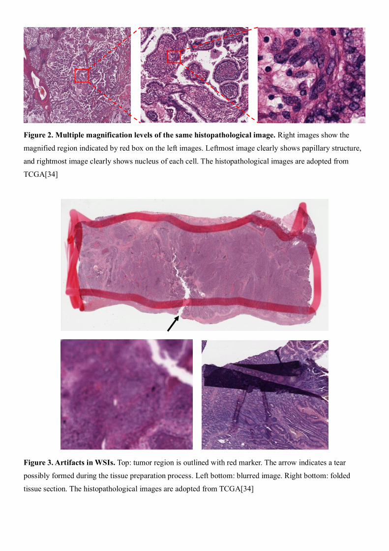
Figure 2. Multiple magnification levels of the same histopathological image. Right images show the
magnified region indicated by red box on the left images. Leftmost image clearly shows papillary structure,
and rightmost image clearly shows nucleus of each cell. The histopathological images are adopted from
TCGA[34]
Figure 3. Artifacts in WSIs. Top: tumor region is outlined with red marker. The arrow indicates a tear
possibly formed during the tissue preparation process. Left bottom: blurred image. Right bottom: folded
tissue section. The histopathological images are adopted from TCGA[34]

Figure 4. Color variation of histopathological images. Both of these two images show lymphocytes. The
histopathological images are adopted from TCGA[34]