Facultad de Ciencias

MACHINE LEARNING METHODS FOR THE

PREDICTION OF NON-METALLIC INCLUSIONS IN STEEL WIRES FOR TIRE

REINFORCEMENT. (Métodos machine learning para la predicción

de inclusiones no metálicas en alambres de acero para refuerzo de neumáticos.)

Trabajo de Fin de Máster para acceder al

MÁSTER EN DATA SCIENCE

Autor: Estela Ruiz Martínez

Director\es: Lara Lloret

Julio - 2019

INDEX

1  INTRODUCTION. ................................................................ 6 

2  MATERIAL AND METHODS. ......................................... 10 

2.1  Steel for tire reinforcement. ......................................................... 10 

2.1.1  Classification of inclusions. .................................................................... 11 

2.1.2  Quality control against non-metallic inclusions. .................................. 13 

2.2  Features, algorithms, imbalanced datasets. ............................... 14 

2.2.1  Features. .................................................................................................. 14 

2.2.2  Algorithms. .............................................................................................. 16 

2.2.3  Imbalanced datasets. .............................................................................. 19 

3  RESULTS AND DISCUSSION. ......................................... 21 

3.1  Evaluation of Machine Learning algorithms. ............................ 21 

3.2  Feature importance. ..................................................................... 26 

3.3  Business impact. ............................................................................ 29 

4  CONCLUSIONS. ................................................................. 31 

5  BIBLIOGRAPHY. .............................................................. 32 

 

   

ACKNOWLEDGMENTS.

This Project was carried out with the financial grant of the program I+C=+C, 2017,

FOMENTO de la TRANSFERENCIA TECNOLÓGICA. The financial contribution

from SODERCAN and the European Union through the program FEDER Cantabria are

gratefully acknowledged. The authors would also like to express their gratitude to the

technical staff of GLOBAL STEEL WIRE and, specially, to Mr. Rafael Piedra, Mr.

Santiago Pascual and Mr. Jean-Francois Fourquet, without whom it would not have

been possible to conduct this research.

ABSTRACT.

Non-metallic inclusions are unavoidably produced during steel casting resulting in

lower mechanical strength and other detrimental effects. This study was aimed at

developing a reliable Machine Learning algorithm to classify castings of steel for tire

reinforcement depending on the number and properties of inclusions, experimentally

determined.

855 observations were available for training, validation and testing the algorithms,

obtained from the quality control of the steel. 140 parameters are monitored during

fabrication, which are the features of the analysis; the output is 1 or 0 depending on

whether the casting is rejected or not.

The following algorithms have been employed: Logistic Regression, K-Nearest

Neighbors, Support Vector Classifier (linear and RBF kernels), Random Forests,

AdaBoost, Gradient Boosting and Artificial Neural Networks. The reduced value of the

rejection rate implies that classification must be carried out on an imbalanced dataset.

Resampling methods and specific scores for imbalanced datasets (Recall, Precision and

AUC rather than Accuracy) were used. Random Forest was the most successful method

providing an AUC in the test set of 0.85. No significant improvements were detected

after resampling.

The improvement derived from implementing this algorithm in the sampling procedure

for quality control during steelmaking has been quantified. In this sense, it has been

proved that this tool allows the samples with a higher probability of being rejected to be

selected, thus improving the effectiveness of the quality control. In addition, the

optimized Random Forest has enabled to identify the most important features, which

have been satisfactorily interpreted on a metallurgical basis.

KEYWORDS.

Machine learning; steel wire; continuous casting; non-metallic inclusions; Random

Forest; imbalanced dataset.

RESUMEN.

Las inclusiones no metálicas se producen inevitablemente durante la fabricación del

acero, lo que resulta en una menor resistencia mecánica y otros efectos perjudiciales. El

objetivo de este estudio fue desarrollar un algoritmo fiable para clasificar las coladas de

acero de refuerzo de neumáticos en función del número y el tipo de las inclusiones,

determinadas experimentalmente.

Se dispuso de 855 observaciones para el entrenamiento, validación y test de los

algoritmos, obtenidos a partir del control de calidad del acero. Durante la fabricación se

controlan 140 parámetros, que son las características del análisis; el resultado es 1 ó 0

dependiendo de si la colada es rechazada o no.

Se han empleado los siguientes algoritmos: Regresión Logística, Vecinos K-Cercanos,

Clasificador de Vectores Soporte (kernels lineales y RBF), Bosques Aleatorios,

AdaBoost, Gradient Boosting y Redes Neurales Artificiales. El bajo índice de rechazo

implica que la clasificación debe llevarse a cabo en un set de datos desequilibrado. Se

utilizaron métodos de remuestreo y métricas específicas para conjuntos de datos

desequilibrados (Recall, Precision y AUC en lugar de Accuracy). Random Forest fue el

algoritmo más exitoso que proporcionó un AUC en los datos de test de 0.83. No se

detectaron mejoras significativas después del remuestreo.

Se ha cuantificado la mejora derivada de la implementación de este algoritmo en el

procedimiento de muestreo para el control de calidad durante la fabricación de acero. En

este sentido, se ha comprobado que esta herramienta permite seleccionar las muestras

con mayor probabilidad de ser rechazadas, mejorando así la eficacia del control de

calidad. Además, el Random Forest optimizado ha permitido identificar las variables

más importantes, que han sido interpretadas satisfactoriamente sobre una base

metalúrgica.

PALABRAS CLAVE.

Aprendizaje automático; alambrón de acero; colada continua; inclusiones no metálicas;

Random Forest; conjunto de datos desequilibrado.

1 INTRODUCTION.  

Monitoring the final properties of steel manufactured products is an indispensable

procedure to guarantee their final quality. After the fabrication of steel, several

properties (such as composition, mechanical behavior or microstructure) are determined

to verify that the quality requirements stated by the product specifications are satisfied.

Steelmaking is an extraordinarily complex process, involving chemical reactions

extremely sensitive to the environmental conditions (temperature, composition, mass

and heat transfer processes, etc.). For this reason, the relationship between the input

parameters of the process and the outcome is highly complex and non-linear. Modelling

these phenomena is very difficult since it involves synergies between input variables

that are unknown in most cases.

Traditionally, science and technology have evolved by applying a bottom-up or

reductionist approach, consisting of breaking down complex physical processes into

smaller and simpler elements that could be easily described through theoretical models.

Then, these low scale models are employed to explain larger scale phenomena. As an

example, high-energy physics is the ground for atomic physics which, in turn, is the

basis of chemistry and solid state physics. The successes achieved by science through

this approach are indisputable. However, this methodology is of limited use in many

industrial processes. As stated in (Wuest et al. 2014), “Traditional methods based on

modelling of cause-effect relations reaches its limits due to the fast increasing

complexity and high-dimensionality of modern manufacturing programmes”. The

manufacture of steel wire in continuous casting, analyzed in this study, represents a

good example. During steelmaking non-metallic inclusions (NMIs) are generated,

which may result in lower mechanical strength and poorer machinability of the steel.

The quantity and nature of such inclusions is determined experimentally from the

quality control conducted on random samples on the final steel. It would be extremely

valuable to have a tool capable of predicting the final quality of the steel from the

manufacturing parameters, which is the scope of the present paper.

The specialized literature offers numerous examples where traditional procedures are

proposed, based on the combination of experimental information and theoretical models

to improve the final quality of steel. Bayesian Networks for classification were used in

(Bustillo and Correa 2012) to optimize the roughness quality after deep drilling for the

manufacture of steel components. In (Pimenov et al. 2018) artificial intelligence

methods (Random Forests, Multi-Layer Perceptrons, Regression Trees, and radial-based

functions) were developed for real-time prediction of surface roughness based on the

tool wear. According to their results, best performance was achieved by means of

Random Forest. The study carried out in (Çaydaş and Ekici 2012) shows that support

vector machines outperformed artificial neural network predicting the surface roughness

of AISI 304 stainless steel after turning operation. An exhaustive comparison between

machine learning algorithms to predict the mechanical properties of hot dip galvanized

steel coils is contained in (Ordieres-Meré et al. 2010); as a relevant result, this study

enables to select the most suitable algorithm to predict each of the output variables of

the process. Specific research has been carried out for determining NMIs in steels.

Without claiming to be exhaustive, the following can be mentioned. The authors in

(Wintz et al. 1995) developed a model based on multiphase equilibrium for the

calculation of the precipitation of NMIs during solidification by combining the

microsegregation equations and the equilibrium conditions between liquid steel and

several types of inclusions. By using samples from different steel grades, they obtained

results for sulphides in agreement with the experimental data. In (Choudhary and Ghosh

2009), a computation procedure for the prediction of inclusion compositions formed

during cooling and solidification of liquid steel was developed. The compositions of

inclusions at various solid fractions were determined and the predictions of the model

were compared with data coming from the literature as well as with inclusion

compositions determined in continuously cast billet samples using SEM-EDS, obtaining

an acceptable good agreement. The modeling of inclusion formation was developed by

(You et al. 2017) predicting types and compositions of inclusions in fair agreement with

the experimental results. The prediction of compositions of NMIs during solidification

was addressed by (Lehmann et al. 2001) who took into account microsegregation and

homogeneous nucleation in the interdendritic liquid observing results in agreement to

industrial observations on semi-killed steels. The precipitation of NMIs (complex

oxides, sulphides, nitrides, etc.) during steel solidification was analyzed using a

multiphase equilibrium code and a nucleation and growth model in (Gaye et al. 1999).

The predicted size distribution of TiN precipitates formed in two steel grades was in

good agreement with the results of laboratory experiments. In the case of liquid oxide

precipitation, it was observed that the composition of inclusions could be significantly

different from that of inclusions assumed to precipitate under equilibrium conditions.

The 3D turbulence flow of the steel melt and the trajectories of NMIs was modelled by

(Pfeiler et al. 2005). They confronted the performance of the numerical simulations

comparing two scenarios, namely, the one-way coupling (which considers only the

impact of the melt flow on the trajectories of the dispersed phases) and the two-way

coupling, obtaining better results with this second approach. Due to the detrimental

effects derived from the presence of NMIs, several methods of improving the

cleanliness and NMIs content are available. (L. E. K. Holappa and Helle 1995)

compared different cleaning methods as well as their influence on the mechanical

properties and machinability of steel. The positive consequences of steel cleanliness

were studied too by (B.-H. Yoon, K.-H. Heo 2013), determining the role of different

parameters (such as CaO/Al2O3 ratio, slag basicity, fluidity, and oxygen activity) on the

final properties of steel. The effects of composition, size, number and morphology of

NMIs on machinability factors (such as cutting tool wear, power consumption, etc.)

were discussed and summarized in (Ånmark et al. 2015). In addition, the authors

proposed methods for modification of NMIs in the liquid steel to obtain a desired

balance between mechanical properties and machinability of various steel grades.

All these works as well as many others are worthy of the greatest respect. Their most

outstanding virtue is the development of experimental and/or numerical procedures that

allow the very specific processes behind the formation of NMIs to be understood.

However, for these very same reasons, they are of limited use when it comes to making

reliable predictions between the steel fabrication parameters and the presence of NMIs

in the final product. Next, we mention some successful examples that start from a

different perspective based on the use of Machine Learning (ML) algorithms for the

prediction of the final properties of steel from the manufacturing variables or

complementary treatments. Without claiming to be exhaustive, the following relevant

studies can be cited. (Fileti et al. 2006) developed neural models to a basic oxygen

steelmaking plant to match with the targets of temperature and carbon content in liquid

steel. Their results improved those obtained by means of a commercial model. In

addition, the model was implemented as an inverse engineering tool to obtain a high

level of steel productivity and a reduction in steel reprocessing. The work developed in

(Santos et al. 2003) presents the development of a computational algorithm to maximize

the quality of steel billets produced by continuous casting; the authors employed a

mathematical model of solidification integrated with a genetic search algorithm

comparing its predictions with their own experimental data as well as literature results,

obtaining a good agreement. By employing an artificial intelligence heuristic search

method, (Cheung and Garcia 2001) explored the space of parameter settings in order to

find the optimized cooling conditions which results in defect-free billet production,

obtaining very good results regarding the billet quality and casting performance. In

(Mesa Fernández et al. 2008) the authors used several ML techniques to improve the

control of the manufacturing procedure through a better prediction of the final

temperature reducing the consumption of energy in the electric arc furnace. Their model

was successfully developed by using neural networks as a classifier, and a fuzzy

inference function to return the predicted temperature value. The influence of steel

cleanliness and mechanical strength was addressed by (Yilmaz and Ertunc 2007)

employing generalized regression by means of a neural network. In particular, they

found a reliable correlation between the presence on NMIs and the tensile strength. In

(Deshpande et al. 2013) a systematic data driven approach supplemented by physics-

based understanding is explored, employing various regression methods with

dimensionality reduction and ML methods applied to the fatigue properties of steels.

Their results provided insights into the methods studied to make an objective selection

of the appropriate method.

To the best of these authors’ knowledge, no previous study has addressed the prediction

of the NMIs present in a steel manufactured by continuous casting employing ML

algorithms. The processing parameters (inputs or features) were collected over the years

in the context of the quality control program of the Global Steel Wire (GSW, Spain)

company. The amount and characteristics of the NMIs present in the steel (outputs)

were obtained throughout this time by the LADICIM laboratory of the University of

Cantabria. The remainder of this paper is organized as follows: Section 2 (Material and

Methods) describes, (i) the steel wire employed for the manufacture of tire

reinforcement, (ii) the ternary diagrams used to classify NMIs as a function of their

chemistry of NMIs and (iii) the ML algorithms used for the correlation of the input and

output parameters. The experimental results are presented and examined in Section 3

and, finally, the main conclusions achieved are compiled in Section 4.

2 MATERIAL AND METHODS.

2.1 Steel for tire reinforcement.

Steel cord is a highly demanded material in many industrial applications due to its

extraordinary tensile strength which can exceed 4000 MPa for the smallest diameters

(Kirihara 2011). Without any doubt, its most remarkable application is in the form of

filaments for reinforcement in automobile tires. Its use poses some drawbacks, since its

specific strength is lower than that of other possible reinforcement materials (nylon,

polyester, etc.) increasing the weight of the tires. However, as a counterpart, the steel

wire offers the advantages of high stiffness and excellent thermal conductivity, which

contribute to significantly extending the life of the tires and reducing fuel consumption.

To achieve this excellent mechanical performance, the most suitable alloy steel must be

selected and the manufacturing process must be optimized. With regard to the selection

of steel, the increasingly demanding strength requirements have resulted in the

progressive increase in carbon content from 0.7% (hypoeutectoid steel), 0.8% (eutectoid

steel) and even up to 0.9% (hypereutectoid steel); in all cases pearlite is the optimum

microstructure (Tashiro and Tarui 2003).

Continuous casting is the procedure employed to obtain the steel cord. It is based on the

fusion of raw materials in the electric arc furnace (EAF). The main raw material for the

EAF process is steel scrap but other forms are often employed (such as direct reduced

iron and iron carbide). In addition, some auxiliary materials are commonly incorporated

(fluxes, ferro-alloys, etc.). After the fusion of the raw material, the billet is obtained

through a molding process and then, hot rolling is applied to produce a wire rod with a

diameter of 5.5 mm which is then drawn down to 0.2 mm or less.

These fine filaments are twisted into strands being subjected in this process to

significant stresses that can eventually cause their fracture; for this reason, the strict

quality of the filament is demanded along its entire length (which is in the order of

kms.). Different types of defects may cause the breakage of the wire such as surface

scratches, central segregations, decarburization of the steel and, especially, the presence

of NMIs. Inclusions that are a few tens of microns in size can trigger the cracking

process of a filament, affecting its ductility, fatigue behavior and machinability

(Lambrighs et al. 2010) (Lipiński and Wach 2015) (Atkinson and Shi 2003). The usual

quality standards limit the number of wire fractures during twisting to no more than one

every 100 km (Yan et al. 2014). In addition, inclusions can cause significant

disturbances during the continuous casting process due to the formation of deposits that

result in the clogging of the submerged nozzle. For all these reasons, steel cleaning

directly affects the quality of steel cord for tire reinforcement; consequently the

presence of NMIs must be minimized in order to reduce unexpected breakages

(Millman 2004). The control of steel cleaning involves a rigorous monitoring of NMIs

formed in the liquid metal in terms of chemical composition, abundance, distribution,

morphology and size. The term "Inclusion Engineering" has been coined to bring all

these aspects together in a discipline with its own identity (L. Holappa and Wijk 2014).

The manufacture of steel is a complex process involving many variables and parameters

that directly or indirectly affect the quality of the final product. The composition of the

raw materials, the temperature of the casting, the basicity of the slag, the intensity of the

electromagnetic agitation in the mold or the speed of cooling are only some of the

parameters on which to focus to guarantee the quality and cleanliness of the final

product. This is why the introduction of new approaches based on ML algorithms can

be of great help to optimize steel quality and cleanliness controls, and even provide

predictions about the inclusionary condition of the steel as a function of the values of

these parameters during the manufacturing process.

2.1.1 Classification of inclusions.

NMIs are classified according to their origin as endogenous (or primary) or exogenous

(precipitates). Endogenous inclusions are intentionally formed during the deoxidation

stage and during the cooling and solidification of the liquid metal by reaction between

the dissolved oxygen and some added deoxidizing agents, such as aluminum or silicon.

Exogenous inclusions are the result of undesired interactions between the deoxidized

steel and its environment. They are generally more pernicious due to their larger size,

irregular shapes and sporadic distribution (Van Ende 2010) (You et al. 2017). The

morphology and nature of NMIs condition the mechanical behavior of the resulting

steel. Fig. 1 shows an example of a fractured wire for tire reinforcement in which the

failure was provoked by the central NMI that can be seen.

Figure 1. The central NMI present at the central region acted as a stress raiser, leading

to the premature failure of this wire for tire reinforcement.

Steel cord for tire reinforcement is one of the most demanding products in terms of

inclusionary cleaning, with very restrictive requirements in relation to the maximum

allowable size of NMIs (which depends on the carbon content, C (wt.): 5 m for

C=0.80–0.85%, 10 m for C=0.7–0.75% and 20 m for C<0.7%) (Zhang and Thomas

2006).

The presence of inclusions containing (Al2O3) is determinant for the performance of

the steel since the deformability of an inclusion is significantly affected by the Al2O3

content. Inclusions containing 20% alumina enjoy optimal deformability (Maeda et al.

1989). Several techniques can be employed to mitigate the detrimental effect of Al2O3.

Thus, calcium treatment transforms alumina inclusions (Al2O3) into low melting

calcium aluminates, which are globular and less abrasive than Al2O3 at the rolling

temperatures (Cui and Chen 2012) (Chen et al. 2012). In addition, a low-basicity slag

favors the formation of deformable inclusions. When the basicity CaO / SiO2 = 0.8 -

1.5, the aluminum dissolved in the steel should be 1-5 ppm to achieve 20% Al2O3 in

the inclusions (Zhang and Thomas 2006).

2.1.2 Quality control against non-metallic inclusions.  

Steel mills worldwide follow a set of protocols in the manufacture of tire steel cord to

achieve the specified compositional ranges of steel and its cleaning requirements, with

special attention to the quantity, size, shape and distribution of the population of NMIs.

During casting, the following procedures are commonly applied:

Deoxidation.

Slag refining.

Use of special fluxes in the tundish and in the mold.

Selection of the refractory of the ladle furnace and the tundish.

Protection of the discharge of the molten steel, controlling the level and

temperature in the molds of the continuous casting process.

Use of electromagnetic stirring in the mold.

In addition, steel mills have internal quality assurance procedures for the control of

NMIs. The GSW protocol is based on the characterization of samples taken from

randomly selected castings by means of scanning electron microscopy (SEM) and

microanalysis (EDX) techniques. For each casting, six samples are obtained from 5.5

mm wire rods from different rolls and examined in the SEM after appropriate

metallographic preparation. An area of 6.86 mm2 (1.14 mm2 per sample) is randomly

chosen and all the inclusions larger than 1 μm in size are quantitatively analyzed. The

report includes the total number of inclusions, the distribution of sizes and the

composition of each inclusion which is represented within the ternary diagram Al2O3 /

SiO2 / CaO + MgO + MnO, as shown in Fig. 2). The ternary diagram is divided into

three regions, A, B and C. According to the quality protocol, there is a maximum limit

to the percentage of particles allowable in regions B and C. Otherwise, the casting

should be rejected (‘non-accepted’). Fig. 2 shows an example of a ternary diagram

where 100, 102 and 20 NMIs were classified in regions A, B and C, respectively.

Figure 2. Example of a ternary diagram where 100, 102 and 20 NMIs were classified in

regions A, B and C, respectively.

It seems evident that the availability of tools that help to foresee the inclusionary

condition as a function of the manufacturing parameters should allow the final quality

of the steel cord to be improved. In this sense, as will be shown in the following

sections, the algorithms based on ML methods represent a substantial advance that

brings new perspectives to the steelmaking process.

2.2 Features, algorithms, imbalanced datasets.

2.2.1 Features.

This study is aimed at developing and validating a classification algorithm based on ML

techniques to identify non-accepted castings (according to the criteria described above)

based on the fabrication parameters. During the manufacture of the steel for tire

reinforcement, 140 parameters are monitored, which can be classified according to the

phases of the fabrication process. Steelmaking consists of three consecutive stages:

Electric arc furnace (EAF), ladle furnace (LF) –or secondary metallurgy– and

continuous casting (CC). The EAF is fed with recycled scrap, direct reduced iron (DRI),

and hot briquetted iron (HBI), which are melted to produce liquid steel with the required

chemistry and temperature. A crucial part of steelmaking is the formation of slag, which

floats on the surface of the molten steel. Slag favors the refining of steel, acting as a

destination for oxidized impurities, and reduces excessive heat loss. Lime and dolomite

are purposely included in the charge of the EAF, to promote the formation of slag. The

final stage in the EAF is the tapping of the liquid steel into the transportation ladle,

previously preheated according to the production protocol. During tapping, ferroalloys

and additives are added to the ladle to build a new slag layer. The following 23

parameters are measured in the EAF stage:

Chemistry of the steel (20 chemical elements: C, Mn, Si, P, S, Cr, Ni, Cu, Mo,

Sn, V, N, Al, B, Ti, Pb, Bi, Nb, Ca and Se) at the end of the stage.

Waiting time of the ladle after tapping until starting the next stage (minutes).

Temperature of steel during tapping (ºC).

Amount of oxygen in the steel during tapping (which measures its level of

oxidation).

The LF is composed of the transportation ladle after coupling to a lid that seals the

vessel. The LF consists of an electrode-based heating system to maintain the

temperature of the liquid steel during processing. Argon gas is injected from the bottom

of the melt for stirring. Ladle slag is refined in the LF to increase the cleanliness of the

liquid steel (i.e. to absorb and chemically bind sulphur from the steel), to absorb NMIs,

to protect the steel from the atmosphere and to minimize heat losses. The following 93

parameters are determined at the LF stage:

The chemistry of the steel (20 chemical elements: C, Mn, Si, P, S, Cr, Ni, Cu,

Mo, Sn, V, N, Al, B, Ti, Pb, Bi, Nb, Ca and Se) is obtained at three different

moments at the LF.

Entrance and exit temperatures of the steel at the LF.

The chemical composition of the slag is determined at the entrance and exit,

measuring the amount (% weight) of 12 oxides (CaO, SiO2, Al2O3, MgO,

Fe2O3, K2O, MnO, Na2O, Cr2O3, P2O5, SO3 and TiO2).

The basicity of the slag is obtained at the entrance and exit.

Heating time of the steel (s).

Amount of fluxes added to the slag.

Argon flow during stirring (l/min).

Argon injection time (s).

Number of consecutive uses of the LF.

Then, the ladle with liquid steel is transported to the CC unit, which is responsible for

the transformation of steel into slabs. This operation uses the force of gravity to pour the

liquid steel in the tundish, fill the mold and help to move along the continuous metal

casting. During CC, the following 24 parameters are measured:

The chemistry of the steel (20 chemical elements: C, Mn, Si, P, S, Cr, Ni, Cu,

Mo, Sn, V, N, Al, B, Ti, Pb, Bi, Nb, Ca and Se) is obtained at the tundish.

Three representative temperatures are recorded at the tundish (after 5, 20 and 50

minutes).

Number of previous consecutive castings in the tundish.

These numeric parameters are the features of the classification algorithm. The targets

are represented by the results of the ternary diagrams experimentally obtained after

fabricating the steel. The most relevant result is the acceptance or rejection of the

casting. The data used in this study included 855 observations (castings), 793 of which

were classified as ‘accepted’ (class 0) and the rest as ‘non-accepted’ (class 1). The

rejection rate of the process is therefore 7.25%.

2.2.2 Algorithms.  

The ML models have been developed and evaluated in Python using the libraries

numpy, pandas, scikit-learn, matplotlib and seaborn. During the feature engineering

stage, missing data were replaced by the average value for that variable. Before

processing, features were standardized to make them have zero-mean and unit-variance.

This technique is generally recommended and mandatory when employing some

specific algorithms. The following classification algorithms have been used in this

research:

Logistic regression (LR): LR is one of the most used ML algorithms for binary

classification that can be used as a performance baseline. LR measures the linear

relationship between the dependent variable and the independent variables, by

estimating probabilities using the sigmoid / logistic function (which is

determined through a Maximum Likelihood Method). The logistic function

returns the probability of every observation to belong to class 1. This real value

in the interval (0, 1) is transformed into either 0 or 1 using a threshold value.

K-Nearest Neighbors (KNN): In KNN, classification or regression are

conducted for a new observation by summarizing the output variable of the ‘K’

closest observations (the neighbors) with uniform weights or with weights

proportional to the inverse of the distance from the query point. Classification is

carried out using the mode of the neighbors while regression is usually based on

the mean. The simplest method to determine the closeness to neighbor instances

is to use the Euclidean distance. KNN suffers the so-called curse of

dimensionality; in this case, the performance of the algorithm may fail in

problems with a large number of input variables (high dimension).

Support Vector Machines (SVM): SVM was originally designed as a classifier

(Vapnik and Chervonenkis 1964) but may also be used for regression and

feature selection. In classification, SVM determines the optimal separating

hyperplane between linearly separable classes maximizing the margin, which is

defined as the distance between the hyperplane and the closest points on both

sides (classes). For non-perfectly separable classes, SVM must be modified to

allow some points to be misclassified, which is achieved by introducing a “soft

margin” (Mohamed 2007). However, many datasets are highly nonlinear but can

be linearly separated after being nonlinearly mapped into a higher dimensional

space (Boser et al. 1992). This mapping gives rise to the kernel, which can be

chosen by the user among different options such as linear, sigmoid, Gaussian or

polynomial; the appropriate kernel function is selected by trial and error on the

test set. In this case, SVM is referred to as kernelized SVM.

Algorithmic Ensemble Techniques: Ensemble methods combine multiple “weak

classifiers” into a single “strong classifier”. A weak classifier is a classifier that

performs poorly, but performs better than random guessing. Ensemble methods

are classified into bagging-based and boosting-based, which are designed to

reduce variance and bias, respectively. Bagging stands for Bootstrap

Aggregating. Random forest (RF) is a widely used bagging method based on

classification trees (weak learner). In RFs, each tree in the ensemble is built

from a sample drawn with replacement (i.e. a bootstrap sample) from the

training set. In addition, instead of using all the features, a random subset of

features is selected, further randomizing the tree. AdaBoost (AB), which stands

for adaptive boosting, is the most widely used form of boosting algorithm. In

this case, weak learners are trained sequentially, each one trying to correct its

predecessor. In AB, the weak learners are usually decision trees with a single

split, called decision stumps. When AB creates its first decision stump, all

observations are weighted equally. In the next step, the observations that were

incorrectly classified are assigned more weight than those that were correctly

classified. AB algorithms can be used for both classification and regression

problems. One drawback of this technique is that it cannot be parallelized and,

as a result, it does not scale as well as bagging. Gradient Boosting (GB) is

another ensemble algorithm, very similar to AB, which works by adding

predictors sequentially to a set, each correcting its predecessor. However,

instead of adjusting the weights of the instances for each new predictor, as AB

does, this method tries to adjust the new predictor to the residual errors of the

previous predictor.

Artificial Neural Networks (ANN): ANNs are mostly used for data classification

and pattern recognition. A basic ANN contains a large number of neurons /

nodes arranged in layers. A Multi-Layer Perceptron (MLP) contains one or more

hidden layers (apart from one input and one output layers). The nodes of

consecutive layers are connected and these connections have weights associated

with them. In a feedforward network, the information moves in one direction

from the input nodes, through the hidden nodes (if any) to the output nodes. The

output of every neuron is obtained by applying an activation function to the

linear combination of inputs (weights) to the neuron; sigmoid, tanh and ReLu

(Rectified Linear Unit) are the most widely used activation functions. MLPs are

trained through the backpropagation algorithm. Gradient descent, Newton,

conjugate gradient and Levenberg-Marquardt are different algorithms to train an

ANN.

2.2.3 Imbalanced datasets.

The number of ‘rejected’ castings (class 1) in this dataset is significantly lower than the

set of ‘accepted’ castings (class 0) with a rejection rate of 7.25%. This scenario

corresponds to an imbalanced class distribution, common in anomaly detection. In this

situation, standard classifier algorithms tend to predict the majority class data ignoring

the minority class, which are frequently considered as noise. The scores used to evaluate

the performance of a classification algorithm may be strongly biased in imbalanced

datasets. Accuracy is the most widely used score in classification, which is defined as

the ratio of correct predictions to the total number of instances evaluated, see Eq. (1).

𝐴𝑐𝑐𝑢𝑟𝑎𝑐𝑦 (1)

where TP, TN, FP and FN are the number of true positives, true negatives, false

positives and false negatives, respectively.

However, by virtue of the so-called “accuracy paradox”, a predictive model may have

high accuracy, but be useless. The paradox lies in the fact that for imbalanced sets,

accuracy can be improved by always predicting negative (‘accepted’ in this case). In

extreme cases, a predictive model with low accuracy may have higher predictive power

than one with high accuracy. There are different methods for dealing with imbalanced

sets, which may be categorized as follows:

Resampling techniques: This strategy consists in preprocessing the data to

balance the classes in the data before using them as input for the learning

algorithm. There are two approaches, increasing the frequency of the minority

class (random oversampling) or decreasing the frequency of the majority class

(random undersampling). In both cases, after resampling approximately the

same number of instances are obtained for both classes.

Alternative scores: A confusion matrix is a table with two rows and two columns

that reports the predicted and the actual instances, providing the number of FPs,

FNs, TPs and TNs. This allows more detailed analysis than Accuracy. Recall

and Precision are robust scores for imbalanced samples. Recall (also called

Sensitivity, Hit Rate or True Positive Rate, TPR), see Eq. (2), measures the

ability of a model to find all the relevant cases within a dataset. Recall can be

thought of as a measure of the completeness of a classifier. Low Recall indicates

many FNs. Precision, see Eq. (3), is the ability of the classifier to identify only

the relevant data points. Precision is a measure of the exactness of a classifier.

Low Precision indicates a large number of FPs. While Recall expresses the

ability to find all relevant instances in a dataset, Precision expresses the

proportion of relevant data points the model predicted to be relevant. Often,

there is a trade-off between Precision and Recall, where it is possible to increase

one at the cost of reducing the other. The Receiver Operating Characteristic

(ROC) curve is a graphical representation to show the performance of a

classification model. An ROC curve plots the Recall (or TPR) on the y-axis

versus the False Positive Rate (FPR=FP/(FP+TN) or Specificity), which is the

probability of a false alarm, on the x-axis. A typical ROC curve is shown below,

see Fig. 3. The continuous diagonal line indicates a random classifier and the

discontinuous curve shows a classification model that improves random

guessing. For a given model, adjusting the threshold makes it possible to move

along the curve (reducing the threshold means moving to the right and upwards

along the curve). The ROC curve results can be synthesized numerically by

calculating the total Area Under the Curve (AUC), a metric which falls between

0 and 1 with a higher number indicating better classification performance. For a

random classifier AUC = 0.5 while for a perfect one, AUC=1.0.

𝑅𝑒𝑐𝑎𝑙𝑙 (2)

𝑃𝑟𝑒𝑐𝑖𝑠𝑖𝑜𝑛 (3)

Ensemble methods: The use of ensembles has been studied in the context of

imbalanced datasets in classification. Thus, (Galar et al. 2012) have studied the

combination between resampling techniques with bagging or boosting

ensembles. Their results show that ensemble-based algorithms outperform the

use of resampling before learning the classifier.

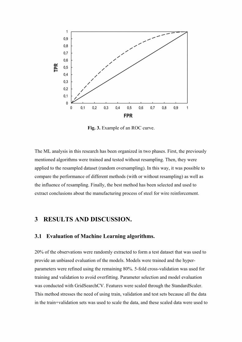
Fig. 3. Example of an ROC curve.

The ML analysis in this research has been organized in two phases. First, the previously

mentioned algorithms were trained and tested without resampling. Then, they were

applied to the resampled dataset (random oversampling). In this way, it was possible to

compare the performance of different methods (with or without resampling) as well as

the influence of resampling. Finally, the best method has been selected and used to

extract conclusions about the manufacturing process of steel for wire reinforcement.

3 RESULTS AND DISCUSSION.

3.1 Evaluation of Machine Learning algorithms.

20% of the observations were randomly extracted to form a test dataset that was used to

provide an unbiased evaluation of the models. Models were trained and the hyper-

parameters were refined using the remaining 80%. 5-fold cross-validation was used for

training and validation to avoid overfitting. Parameter selection and model evaluation

was conducted with GridSearchCV. Features were scaled through the StandardScaler.

This method stresses the need of using train, validation and test sets because all the data

in the train+validation sets was used to scale the data, and these scaled data were used to

run the grid search using 5-fold CV. For each split, some part of the original training set

will be considered as the validation part of the split introducing information contained

in the train part of the split when scaling the data. To avoid this problem, the splitting of

the dataset during cross-validation was done before undertaking any preprocessing

(including the scale of features) (Guido and Müller 2016).

Next, the main characteristics of the algorithms employed after tuning are described:

Logistic regression, LR: For the best hyper-parameters of the model, the ‘saga’

solver was selected with an L1 penalty. A strong regularization was achieved

with C=0.1; tol=1e-5 was selected as the optimum tolerance value for stopping

criteria. Finally, a maximum number of 10000 interactions guaranteed

convergence.

K-Nearest Neighbors, KNN: The optimum number of neighbors found was 7,

and the best distance metric was manhattan (minkowski with p=1). The

algorithm used to compute the nearest neighbors was BallTree with a leaf size of

10. Finally, the weight of the points was considered by the inverse of their

distance to the query point.

SVM: the linear kernel was used as a baseline model. Then, the Radial Basis

Function (RBF) kernel was fine-tuned determining the best combination of

parameters C and gamma through grid search, to obtain C=20 and gamma=0.01.

Random Forest, RF: The optimum number of decision trees in the forest was

750; ‘entropy’ was the function to measure the quality of a split.

AdaBoost, AB: The optimum number of estimators (decision trees with max

deep of 1) was 15 with a learning rate of 0.5. The algorithm used was

SAMME.R.

Gradient Boosting, GB: The optimum number of boosting stages was 1200 with

a learning rate of 0.01 that shrinks the contribution of each tree and a fraction of

samples to be used for fitting each individual base learner (subsample) of 0.5.

The maximum depth of the individual estimators was 3 which limits the number

of nodes in each tree.

Artificial Neural Networks, ANN: the optimum MLP consisted in two hidden

layers with 10 nodes each. The activation function was ReLu. The Learning rate

was established as ‘invscaling’, which gradually decreases the learning rate. An

L2 penalty of alpha=0.1 was applied as a regularization term to prevent

overfitting.

The results obtained with each of the algorithms are summarized hereafter. Table 1 and

Table 2 show the Accuracy and AUC on the original dataset and after oversampling,

respectively. In both cases, the scores were calculated for the train+validation set and

for the test set, respectively. The train+validation data shows the mean value and the

95% confidence interval of the estimation of each metric (obtained from the 5 results of

the cross validation).

Table 1: Accuracy and AUC scores for the train+validation and test sets. Original

dataset.

Train + validation Test

Model Accuracy AUC Accuracy AUC

LR 0.93 ± 0.01 0.78 ± 0.09 0.90 0.78

KNN 0.93 ± 0.01 0.70 ± 0.10 0.91 0.73

SVC

(RBF)

0.94 ± 0.01 0.81 ± 0.10 0.92 0.78

SVC

(linear)

0.87 ± 0.03 0.69 ± 0.14 0.83 0.73

RF 0.93 ± 0.01 0.83 ± 0.13 0.91 0.85

AB 0.93 ± 0.03 0.84 ± 0.18 0.89 0.82

GB 0.93 ± 0.03 0.80 ± 0.20 0.91 0.79

ANN 0.91 ± 0.02 0.73 ± 0.08 0.91 0.79

Table 2: Accuracy and AUC scores for the train+validation and test sets. Resampled

dataset.

Train + validation Test

Model Accuracy AUC Accuracy AUC

LR 0.90 ± 0.03 0.95 ± 0.02 0.78 0.76

KNN 0.90 ± 0.02 0.98 ± 0.01 0.81 0.74

SVC

(RBF)

1.00 ± 0.00 1.00 ± 1.00 0.91 0.78

SVC

(linear)

0.95 ± 0.02 0.93 ± 0.01 0.82 0.73

RF 1.00 ± 0.00 1.00 ± 0.00 0.92 0.83

AB 0.89 ± 0.03 0.96 ± 0.02 0.82 0.77

GB 0.98 ± 0.01 1.00 ± 0.00 0.91 0.79

ANN 0.97 ± 0.01 0.99 ± 0.02 0.88 0.79

The most significant outcomes are summarized below:

As expected, Accuracy is a substantially insensitive metric for imbalanced

datasets, which offers deceptively optimistic results. Taking into account the

rejection rate, 7.25%, a model predicting only negative results (that is to say, not

classifying any instance as class 1) would offer an Accuracy of 0.9275.

Note that the performance of the algorithms is not improved after using

oversampling. Rather, the scores obtained in the train+validation set after

resampling are very high but noticeably lower in the test set. This is an

unmistakable symptom of overfitting. This outcome is not surprising because

oversampling may increase the likelihood of overfitting since it replicates the

minority class events (Mukherjee 2017).

AUC does not suffer from the limitations of Accuracy and allows the most

appropriate algorithm to be selected. The best results (in the non-resampled

dataset) are obtained through the RF algorithm. The AUC for the

train+validation set amounts to 0.83 ± 0.13 while for the test set it is 0.85. KNN

and SVC (linear) are the poorest algorithms for classification (AUC=0.78 in

both cases). According to (Guido and Müller 2016), the AUC=0.85 is equivalent

to a probability of 85% that a randomly picked point of the positive class

(rejected casting) will have a higher score according to the classifier than a

randomly picked point from the negative class (non-rejected casting). Fig. 4

shows a comparison between the ROC curves provided by RF in the original

dataset and after applying resampling. As can be seen, this technique does not

represent any perceptible improvement in this case.

Fig. 4. ROC curves obtained with RF with and without resampling.

It is a well-known fact that there is a trade-off between the Precision and Recall

scores. This fact is represented in Fig. 5 where the curves of both metrics as a

function of the threshold obtained by means of RF are represented, considering

the original dataset (Fig. 5(a)) and the dataset subjected to resampling (Fig.

5(b)).

(a)

(b)

Fig. 5. Relationship between Precision and Recall scores as a function of the threshold

using (a) the original dataset and (b) after resampling.

To carry out a final evaluation of the selected classifier, completely independent of the

results shown above, 149 additional castings (different from those that formed the

train+validation and test sets) have been considered. Three of these new instances were

rejected based on the experimental results (SEM analysis). The features (input

parameters) of these 149 instances have been introduced in the optimized RF algorithm

and the results have been sorted in descending order of the probability of belonging to

class 1. According to the result obtained through the optimized RF, these three castings

have been classified in positions 3, 10 and 43, with failure probabilities of 26%, 21%

and 11%, respectively.

3.2 Feature importance.

Scikit-learn enables to compute the importance of a node in a decision tree, making it

possible to obtain the importance of a feature. In RF (as in GB), feature importance is

the average over all the trees. After tuning the RF, this method has been used to extract

information regarding the most influential processing parameters; thus, the following

four features were obtained: number of uses of the ladle, amount of Al2O3 and SiO2 in

the slag and amount of carbon in the final steel. Their relevance is next analyzed based

on metallurgical grounds.

Number of uses of the ladle: Each casting is processed with a certain ladle. This

variable represents the number of castings manufactured by that ladle up to that

moment. The bar graph shown in Fig.6 allows the influence of this variable to be

fully appreciated. As can be seen, not only the absolute value but also the

proportion of rejected castings decreases sharply with the number of uses of the

ladle. The ladles used to manufacture steel for tire reinforcement have been

previously used with other qualities of steel; therefore, when changing material,

the ladle is slightly contaminated by strange chemical elements coming from the

previous castings. As more castings for tire reinforcement are processed, this

effect disappears, justifying in this way the importance of this variable in the

presence of undesirable inclusions.

Fig. 6. Bar graph showing the influence between the number of uses of the ladle furnace

and the number of rejected castings.

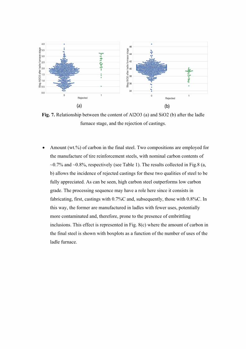
Amount (wt.%) of Al2O3 and SiO2 in the slag at the end of the stage of ladle

furnace. Their influence is represented in Fig.7. Note in Fig.7(a) that the number

of rejected castings (class 1) is concentrated in the region corresponding to high

values of Al2O3 and, as shown in Fig.7(b), to low and medium values of SiO2.

The relationship between these compositional variables and the final presence of

inclusions is evident since the role of the slag is precisely to capture as many

inclusions as possible. As seen above, Al2O3 and SiO2 are two of the vertices

that define a ternary diagram.

(a)

(b)

Fig. 7. Relationship between the content of Al2O3 (a) and SiO2 (b) after the ladle

furnace stage, and the rejection of castings.

Amount (wt.%) of carbon in the final steel. Two compositions are employed for

the manufacture of tire reinforcement steels, with nominal carbon contents of

~0.7% and ~0.8%, respectively (see Table 1). The results collected in Fig.8 (a,

b) allows the incidence of rejected castings for these two qualities of steel to be

fully appreciated. As can be seen, high carbon steel outperforms low carbon

grade. The processing sequence may have a role here since it consists in

fabricating, first, castings with 0.7%C and, subsequently, those with 0.8%C. In

this way, the former are manufactured in ladles with fewer uses, potentially

more contaminated and, therefore, prone to the presence of embrittling

inclusions. This effect is represented in Fig. 8(c) where the amount of carbon in

the final steel is shown with boxplots as a function of the number of uses of the

ladle furnace.

(a)

(b)

(c)

Fig. 8. Number of rejected castings for the two steel grades employed with nominal

carbon contents of ~0.7% (a) and ~0.8% (b), respectively. The influence of the number

of uses of the ladle furnace is shown in (c).

3.3 Business impact.

The so-called ‘business impact’ depends on the metric used to measure the quality of

the algorithm as well as the consequences of its mistakes (False Positive or type I error

and False Negative or type II error). In commercial applications, it is possible to assign

monetary values to both kinds of mistakes, which is the meaningful standard for making

business decisions (Guido and Müller 2016).

This research provides an immediate practical application because it enables to optimize

the process of sample selection for the experimental control of NMIs. A hypothetical

example makes it possible to evaluate the advantages that a ML-oriented process of

sample selection may provide. Consider a sample consisting of 1000 castings,

approximately 73 of which, according to the rejection rate, belong to class 1. Setting a

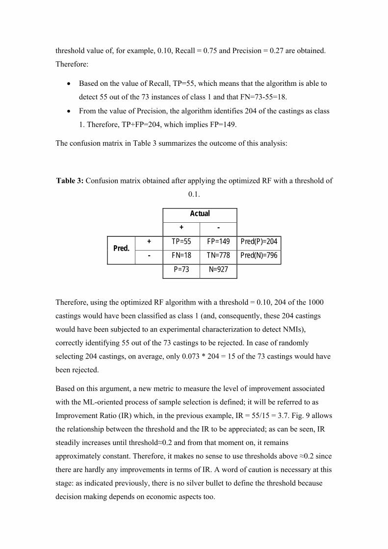
threshold value of, for example, 0.10, Recall = 0.75 and Precision = 0.27 are obtained.

Therefore:

Based on the value of Recall, TP=55, which means that the algorithm is able to

detect 55 out of the 73 instances of class 1 and that FN=73-55=18.

From the value of Precision, the algorithm identifies 204 of the castings as class

1. Therefore, TP+FP=204, which implies FP=149.

The confusion matrix in Table 3 summarizes the outcome of this analysis:

Table 3: Confusion matrix obtained after applying the optimized RF with a threshold of

0.1.

Actual

+ -

Pred. + TP=55 FP=149 Pred(P)=204

- FN=18 TN=778 Pred(N)=796

P=73 N=927

Therefore, using the optimized RF algorithm with a threshold = 0.10, 204 of the 1000

castings would have been classified as class 1 (and, consequently, these 204 castings

would have been subjected to an experimental characterization to detect NMIs),

correctly identifying 55 out of the 73 castings to be rejected. In case of randomly

selecting 204 castings, on average, only 0.073 * 204 = 15 of the 73 castings would have

been rejected.

Based on this argument, a new metric to measure the level of improvement associated

with the ML-oriented process of sample selection is defined; it will be referred to as

Improvement Ratio (IR) which, in the previous example, IR = 55/15 = 3.7. Fig. 9 allows

the relationship between the threshold and the IR to be appreciated; as can be seen, IR

steadily increases until threshold≈0.2 and from that moment on, it remains

approximately constant. Therefore, it makes no sense to use thresholds above ≈0.2 since

there are hardly any improvements in terms of IR. A word of caution is necessary at this

stage: as indicated previously, there is no silver bullet to define the threshold because

decision making depends on economic aspects too.

Fig. 9. Graph showing the relation between the threshold of the RF model (without

resampling) and the Improvement Ratio, IR.

4 CONCLUSIONS.  

The manufacture of steel is an optimum environment for the application of data mining

and machine learning methods, due to the extraordinary complexity of the reactions that

take place during casting. Machine learning algorithms have been used in this research

for the classification of steel castings for tire reinforcement.

Training, validation and testing were conducted using the experimental results, obtained

in the context of the quality program of the factory, consisting of 855 castings. 7.25% of

these 855 castings had been rejected, because of the number and properties of the non-

metallic inclusions present. The following algorithms have been employed: Logistic

Regression, K-Nearest Neighbors, Support Vector Classifier (linear and RBF kernels),

Random Forests, AdaBoost, Gradient Boosting and Artificial Neural Networks (multi-

layer perceptron). Features correspond to the 140 parameters monitored during

steelmaking. The results derived from the quality control (acceptance or rejection) are

the output of the classification. The test dataset was formed by 20% of the observations,

randomly selected; training and validation was conducted on the remaining 80% using

5-fold cross-validation. Different approaches were employed to deal with the

imbalanced class distribution motivated by the small rejection rate, such as resampling

(random oversampling), alternative scores (Precision, Recall and AUC rather than

Accuracy) and ensemble methods (Random Forest, AdaBoost and Gradient Boosting).

The best results were obtained with Random Forest on the non-resampled dataset (AUC

for training+validation equals 0.83 ± 0.13 while for testing it is 0.85). There have been

no improvements after using random oversampling but a slight tendency to overfitting,

which has been previously reported by other authors (Mukherjee 2017).

A numerical example provides insight about the advantages of implementing this

optimized Random Forest in the quality control of castings. With a threshold=0.10,

considering 1000 castings, the algorithm would have predicted 204 observations

belonging to class 1; then, 55 of the approximately 73 castings to be rejected would

have been correctly identified (and rejected). In contrast, random sampling would have

detected only 15 of these 73 castings. A novel metric referred to as Improvement Ratio,

which measures the level of improvement associated with the machine learning-based

procedure of sample selection, has been defined; in this study, the Improvement Ratio

increases until threshold≈0.2 and from that moment on, it remains approximately

constant. Therefore, it makes no sense to use a threshold>0.2 in this dataset. Feature

importance has been used to identify the manufacturing parameters that most affect the

probability of rejecting a casting: number of uses of the ladle, amount of Al2O3 and

SiO2 in the slag and amount of carbon in the final steel. Based on metallurgical

arguments, it has been possible to obtain a coherent picture of the role played by each of

these variables. This achievement represents an example in which machine learning has

enabled to improve the understanding of the physical processes that occur in

manufacturing.

5 BIBLIOGRAPHY.  

Ånmark, N., Karasev, A., & Jönsson, P. G. (2015). The effect of different non-

metallic inclusions on the machinability of steels. Materials, 8(2), 751–783.

doi:10.3390/ma8020751

Atkinson, H. V., & Shi, G. (2003). Characterization of inclusions in clean steels:

A review including the statistics of extremes methods. Progress in Materials

Science, 48(5), 457–520. doi:10.1016/S0079-6425(02)00014-2

B.-H. Yoon, K.-H. Heo, J.-S. K. & H.-S. S. (2013). Improvement of steel

cleanliness by controlling slag composition. Ironmaking & Steelmaking, 29(3),

214–217. doi:10.1179/030192302225004160

Boser, B. E., Guyon, I. M., & Vapnik, V. N. (1992). A training algorithm for

optimal margin classifiers. Proceedings of the fifth annual workshop on

Computational learning theory - COLT ’92, 144–152.

doi:10.1145/130385.130401

Bustillo, A., & Correa, M. (2012). Using artificial intelligence to predict surface

roughness in deep drilling of steel components. Journal of Intelligent

Manufacturing, 23(5), 1893–1902. doi:10.1007/s10845-011-0506-8

Çaydaş, U., & Ekici, S. (2012). Support vector machines models for surface

roughness prediction in CNC turning of AISI 304 austenitic stainless steel.

Journal of Intelligent Manufacturing, 23(3), 639–650. doi:10.1007/s10845-010-

0415-2

Chen, S., Jiang, M., He, X., & Wang, X. (2012). Top slag refining for inclusion

composition transform control in tire cord steel. International Journal of

Minerals, Metallurgy, and Materials, 19(6), 490–498.

doi:https://doi.org/10.1007/s12613-012-0585-3

Cheung, N., & Garcia, A. (2001). Use of a heuristic search technique for the

optimization of quality of steel billets produced by continuous casting.

Engineering Applications of Artificial Intelligence, 14(2), 229–238.

doi:10.1016/S0952-1976(00)00075-0

Choudhary, S. K., & Ghosh, a. (2009). Mathematical Model for Prediction of

Composition of Inclusions Formed during Solidification of Liquid Steel. ISIJ

International, 49(12), 1819–1827. doi:10.2355/isijinternational.49.1819

Cui, H. zhou, & Chen, W. qing. (2012). Effect of Boron on Morphology of

Inclusions in Tire Cord Steel. Journal of Iron and Steel Research International,

19(4), 22–27. doi:10.1016/S1006-706X(12)60082-X

Deshpande, P., Gautham, B., Cecen, A., Kalidindi, S. R., Agrawal, A., &

Choudhary, A. (2013). Application of Statistical and Machine Learning

Techniques for Correlating Properties to Composition and Manufacturing

Processes of Steels. In M. L. C. T. H. Gumbsch (Ed.), 2nd World Congress on

Integrated Computational Materials Engineering (pp. 155–160).

Fileti, A. M. F., Pacianotto, T. A., & Cunha, A. P. (2006). Neural modeling

helps the BOS process to achieve aimed end-point conditions in liquid steel.

Engineering Applications of Artificial Intelligence, 19(1), 9–17.

doi:10.1016/j.engappai.2005.06.002

Galar, M., Fernandez, A., Barrenechea, E., Bustince, H., & Herrera, F. (2012). A

review on ensembles for the class imbalance problem: Bagging-, boosting-, and

hybrid-based approaches. IEEE Transactions on Systems, Man and Cybernetics

Part C: Applications and Reviews, 42(4), 463–484.

doi:10.1109/TSMCC.2011.2161285

Gaye, H., Rocabois, P., Lehmann, J., & Bobadilla, M. (1999). Kinetics of

inclusion precipitation during steel solidification. Steel Research, 70(8), 356–

361. doi:10.1002/srin.199905653

Guido, S., & Müller, A. (2016). Introduction to Machine Learning with Python.

A Guide for Data Scientists. O’Reilly Media.

Holappa, L. E. K., & Helle, A. S. (1995). Inclusion Control in High-

Performance Steels. Journal of Materials Processing Tech., 53(1–2), 177–186.

doi:10.1016/0924-0136(95)01974-J

Holappa, L., & Wijk, O. (2014). Inclusion Engineering. In Treatise on Process

Metallurgy Volume 3: Industrial Processes (pp. 347–372). Elsevier.

Kirihara, K. (2011). Production Technology of Wire Rod for High Tensile

Strength Steel Cord. Kobelco Technology Review, 30, 62–65.

Lambrighs, K., Verpoest, I., Verlinden, B., & Wevers, M. (2010). Influence of

non-metallic inclusions on the fatigue properties of heavily cold drawn steel

wires. Procedia Engineering, 2(1), 173–181. doi:10.1016/j.proeng.2010.03.019

Lehmann, J., Rocabois, P., & Gaye, H. (2001). Kinetic model of non-metallic

inclusions’ precipitation during steel solidification. Journal of Non-Crystalline

Solids, 282(1), 61–71. doi:10.1016/S0022-3093(01)00329-5

Lipiński, T., & Wach, A. (2015). The effect of fine non-metallic inclusions on

the fatigue strength of structural steel. Archives of Metallurgy and Materials,

60(1), 65–69. doi:10.1515/amm-2015-0010

Maeda, S., Soejima, T., & Saito, T. (1989). Shape Control of Inclusions in Wire

Rods for High Tensile Tire Cord by Refining With Synthetic Slag. In ISS (Ed.),

Steelmaking Conference Proceedings (pp. 379–385). Warrendale, PA.

Mesa Fernández, J. M., Cabal, V. A., Montequin, V. R., & Balsera, J. V. (2008).

Online estimation of electric arc furnace tap temperature by using fuzzy neural

networks. Engineering Applications of Artificial Intelligence, 21(7), 1001–1012.

doi:10.1016/j.engappai.2007.11.008

Millman, S. (2004). Clean steel basic features and operation practices. In K.

Wúnnenberg & S. Millman (Eds.), IISI Study on Clean Steel (pp. 39–60).

Brussels, Belgium: IISI Committeee on Technology.

Mohamed, A. E. (2007). Comparative Study of Supervised Machine Learning

Techniques for Intrusion Detection, 14(3), 5–10. doi:10.15546/aeei-2014-0021

Mukherjee, U. (2017). How to handle Imbalanced Classification Problems in

machine learning? Analytics Vidhya.

https://www.analyticsvidhya.com/blog/2017/03/imbalanced-classification-

problem/

Ordieres-Meré, J., Martínez-De-Pisón-Ascacibar, F. J., González-Marcos, A., &

Ortiz-Marcos, I. (2010). Comparison of models created for the prediction of the

mechanical properties of galvanized steel coils. Journal of Intelligent

Manufacturing, 21(4), 403–421. doi:10.1007/s10845-008-0189-y

Pfeiler, C., Wu, M., & Ludwig, A. (2005). Influence of argon gas bubbles and

non-metallic inclusions on the flow behavior in steel continuous casting.

Materials Science and Engineering A, 413–414, 115–120.

doi:10.1016/j.msea.2005.08.178

Pimenov, D. Y., Bustillo, A., & Mikolajczyk, T. (2018). Artificial intelligence

for automatic prediction of required surface roughness by monitoring wear on

face mill teeth. Journal of Intelligent Manufacturing, 29(5), 1045–1061.

doi:10.1007/s10845-017-1381-8

Santos, C. A., Spim, J. A., & Garcia, A. (2003). Mathematical modeling and

optimization strategies (genetic algorithm and knowledge base) applied to the

continuous casting of steel. Engineering Applications of Artificial Intelligence,

16(5–6), 511–527. doi:10.1016/S0952-1976(03)00072-1

Tashiro, H., & Tarui, T. (2003). State of the Art for High Tensile Strength Steel

Cord. Shinnittetsu Giho, (88), 87–91.

http://www.nssmc.com/en/tech/report/nsc/pdf/n8818.pdf

Van Ende, M.-A. (2010). Formation and Morphology of non-Metallic Inclusions

in Aluminium Killed Steels.

Vapnik, V., & Chervonenkis, A. (1964). A note on one class of perceptrons.

Automation and Remote Control, 25.

Wintz, M., Bobadilla, M., Lehmann, J., & Gaye, H. (1995). Experimental Study

and Modeling of the Precipitation of Non-metallic Inclusions during

Solidification of Steel. ISIJ International, 35(6), 715–722.

doi:10.2355/isijinternational.35.715

Wuest, T., Irgens, C., & Thoben, K.-D. (2014). An approach to monitoring

quality in manufacturing using supervised machine learning on product state

data. Journal of Intelligent Manufacturing, 25(5), 1167–1180.

doi:10.1007/s10845-013-0761-y

Yan, W., Xu, H. C., & Chen, W. Q. (2014). Study on inclusions in wire rod of

tire cord steel by means of electrolysis of wire rod. Steel Research International,

85(1), 53–59. doi:10.1002/srin.201300045

Yilmaz, M., & Ertunc, H. M. (2007). The prediction of mechanical behavior for

steel wires and cord materials using neural networks. Materials and Design,

28(2), 599–608. doi:10.1016/j.matdes.2005.07.016

You, D., Michelic, S. K., Presoly, P., Liu, J., & Bernhard, C. (2017). Modeling

Inclusion Formation during Solidification of Steel: A Review. Metals, 7(11),

460. doi:10.3390/met7110460

Zhang, L., & Thomas, B. G. (2006). State of the art in the control of inclusions

during steel ingot casting. Metallurgical and Materials Transactions B, 37(5),

733–761.