machine learning - sharif university of...

Machine LearningOverview of probability

Hamid Beigy

Sharif University of Technology

Spring 1397

Hamid Beigy (Sharif University of Technology) Machine Learning Spring 1397 1 / 26

Table of contents

1 Probability

2 Random variables

3 Variance and and Covariance

4 Probability distributionsDiscrete distributionsContinuous distributions

5 Bayes theorem


Outline

1 Probability

2 Random variables



5 Bayes theorem


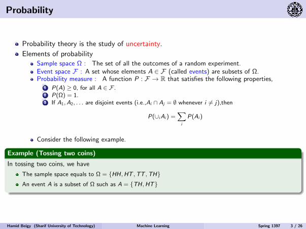
Probability

Probability theory is the study of uncertainty.

Elements of probability

Sample space Ω : The set of all the outcomes of a random experiment.Event space F : A set whose elements A ∈ F (called events) are subsets of Ω.Probability measure : A function P : F → R that satisfies the following properties,

1 P(A) ≥ 0, for all A ∈ F .2 P(Ω) = 1.3 If A1,A2, . . . are disjoint events (i.e.,Ai ∩ Aj = ∅ whenever i = j),then

P(∪iAi ) =∑i

P(Ai )

Consider the following example.

Example (Tossing two coins)

In tossing two coins, we have

The sample space equals to Ω = HH,HT ,TT ,THAn event A is a subset of Ω such as A = TH,HT


Properties of probability

If A ⊆ B =⇒ P(A) ≤ P(B).

P(A ∩ B) ≤ min(P(A),P(B)).

P(A ∪ B) ≤ P(A) + P(B). This property is called union bound.

P(Ω \ A) = 1− P(A).

If A1,A2, . . . ,Ak are disjoint events such that ∪ki=1Ai = Ω,then

k∑i=1

P(Ai ) = 1

This property is called law of total probability.


Probability

Conditional probability and independence

Let B be an event with non-zero probability. The conditional probability of any event Agiven B is defined as,

P(A | B) = P(A ∩ B)

P(B)

In other words, P(A | B) is the probability measure of the event A after observing theoccurrence of event B.

Two events are called independent if and only if

P(A ∩ B) = P(A)P(B),

or equivalently, P(A | B) = P(A).Therefore, independence is equivalent to saying that observing B does not have any effecton the probability of A.


What is probability?

Classical definition (Laplace, 1814)

P(A) =NA

N

where N mutually exclusive equally likely outcomes, NA of which result in the occurrenceof A.

Frequentist definition

P(A) = limN→∞

NA

N

or relative frequency of occurrence of A in infinite number of trials.

Bayesian definition(de Finetti, 1930s)P(A) is a degree of belief.


What is probability? (example)

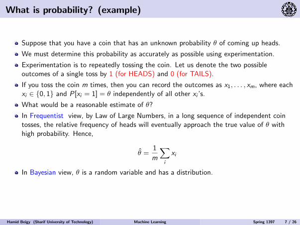
Suppose that you have a coin that has an unknown probability θ of coming up heads.

We must determine this probability as accurately as possible using experimentation.

Experimentation is to repeatedly tossing the coin. Let us denote the two possibleoutcomes of a single toss by 1 (for HEADS) and 0 (for TAILS).

If you toss the coin m times, then you can record the outcomes as x1, . . . , xm, where eachxi ∈ 0, 1 and P[xi = 1] = θ independently of all other xi ’s.

What would be a reasonable estimate of θ?

In Frequentist view, by Law of Large Numbers, in a long sequence of independent cointosses, the relative frequency of heads will eventually approach the true value of θ withhigh probability. Hence,

θ =1

m

∑i

xi

In Bayesian view, θ is a random variable and has a distribution.


Outline

1 Probability

2 Random variables



5 Bayes theorem


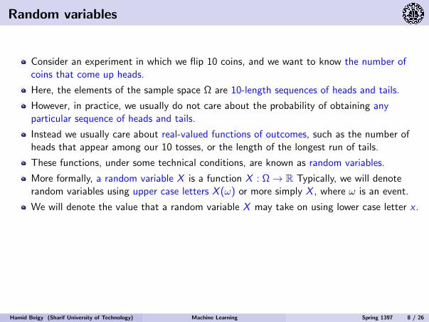
Random variables

Consider an experiment in which we flip 10 coins, and we want to know the number ofcoins that come up heads.

Here, the elements of the sample space Ω are 10-length sequences of heads and tails.

However, in practice, we usually do not care about the probability of obtaining anyparticular sequence of heads and tails.

Instead we usually care about real-valued functions of outcomes, such as the number ofheads that appear among our 10 tosses, or the length of the longest run of tails.

These functions, under some technical conditions, are known as random variables.

More formally, a random variable X is a function X : Ω → R Typically, we will denoterandom variables using upper case letters X (ω) or more simply X , where ω is an event.

We will denote the value that a random variable X may take on using lower case letter x .


Random variables

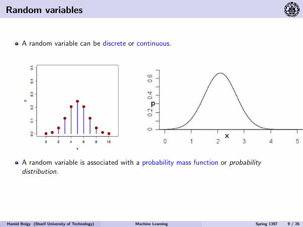
A random variable can be discrete or continuous.

Random Variables

A random variable (r.v.) X denotes possible outcomes of an event

Can be discrete (i.e., finite many possible outcomes) or continuous

Some examples of discrete r.v.

A random variable X 2 0, 1 denoting outcomes of a coin-toss

A random variable X 2 1, 2, . . . , 6 denoteing outcome of a dice roll

Some examples of continuous r.v.

A random variable X 2 (0, 1) denoting the bias of a coin

A random variable X denoting heights of students in CS772

A random variable X denoting time to get to your hall from the department

An r.v. is associated with a probability mass function or prob. distribution

Probabilistic Machine Learning (CS772A) Some Essentials of Probability for Probabilistic Machine Learning 2

A random variable is associated with a probability mass function or probabilitydistribution.


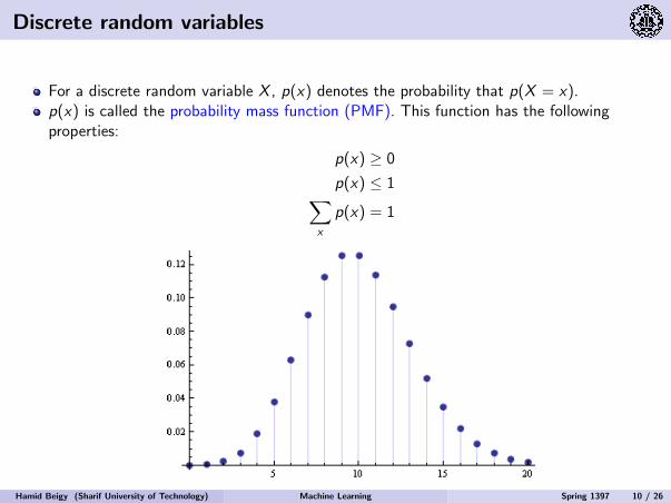
Discrete random variables

For a discrete random variable X , p(x) denotes the probability that p(X = x).p(x) is called the probability mass function (PMF). This function has the followingproperties:

p(x) ≥ 0

p(x) ≤ 1∑x

p(x) = 1

Discrete Random Variables

For a discrete r.v. X , p(x) denotes the probability that p(X = x)

p(x) is called the probability mass function (PMF)

p(x) 0

p(x) 1X

x

p(x) = 1

Picture courtesy: johndcook.com



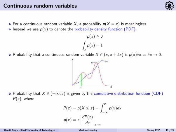
Continuous random variables

For a continuous random variable X , a probability p(X = x) is meaningless.Instead we use p(x) to denote the probability density function (PDF).

p(x) ≥ 0∫xp(x) = 1

Probability that a continuous random variable X ∈ (x , x + δx) is p(x)δx as δx → 0.

Continuous Random Variables

For a continuous r.v. X , a probability p(X = x) is meaningless

Instead we use p(x) to denote the probability density function (PDF)

p(x) 0 and

Z

x

p(x)dx = 1

Probability that a cont. r.v. X 2 (x , x + x) is p(x)x as x ! 0

Probability that X lies between (1, z) is given by the cumulative

distribution function (CDF) P(z) where

P(z) = p(X z) =

Zz

1p(x)dx and p(x) = |P 0(z)|

z=x

Picture courtesy: PRML (Bishop, 2006)


Probability that X ∈ (−∞, z) is given by the cumulative distribution function (CDF)P(z), where

P(z) = p(X ≤ z) =

∫ z

−∞p(x)dx

p(x) = z

∣∣∣∣dP(z)dz

∣∣∣∣z=x


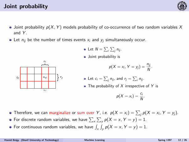
Joint probability

Joint probability p(X ,Y ) models probability of co-occurrence of two random variables Xand Y .

Let nij be the number of times events xi and yj simultaneously occur.

Let N =∑

i

∑j nij .

Joint probability is

p(X = xi ,Y = yj) =nijN

.

Let ci =∑

j nij , and rj =∑

i nij .

The probability of X irrespective of Y is

p(X = xi ) =ciN.

Therefore, we can marginalize or sum over Y , i.e. p(X = xi ) =∑

j p(X = xi ,Y = yj).

For discrete random variables, we have∑

x

∑y p(X = x ,Y = y) = 1.

For continuous random variables, we have∫x

∫y p(X = x ,Y = y) = 1.


Marginalization

Consider only instances where the fraction of instances Y = yj when X = xi .

This is conditional probability and is written p(Y = yj |X = xi ), the probability of Y givenX .

p(Y = yj |X = xi ) =nijci

Now consider

p(X = xi ,Y = yj) =nijN

=nijci

ciN

= p(Y = yj |X = xi )p(X = xi )

If two events are independent, p(X ,Y ) = p(X )p(Y ) and p(X |Y ) = p(X )

Sum rule p(X ) =∑

Y p(X ,Y )

Product rule p(X ,Y ) = p(Y |X )p(X )


Expected value

Expectation, expected value, or mean of a random variable X , denoted by E[X ], is theaverage value of X in a large number of experiments.

E[x ] =∑x

p(x)x

or

E[x ] =∫

p(x)xdx

The definition of Expectation also applies to functions of random variables (e.g., E[f (x)])Linearity of expectation

E[αf (x) + βg(x)] = αE[f (x)] + βE[g(x)]


Outline

1 Probability

2 Random variables



5 Bayes theorem


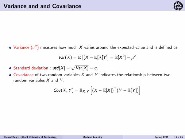
Variance and and Covariance

Variance (σ2) measures how much X varies around the expected value and is defined as.

Var(X ) = E[(X − E[X ])2

]= E[X 2]− µ2

Standard deviation : std [X ] =√

Var [X ] = σ.

Covariance of two random variables X and Y indicates the relationship between tworandom variables X and Y .

Cov(X ,Y ) = EX ,Y

[(X − E[X ])T (Y − E[Y ])

]


Outline

1 Probability

2 Random variables



5 Bayes theorem


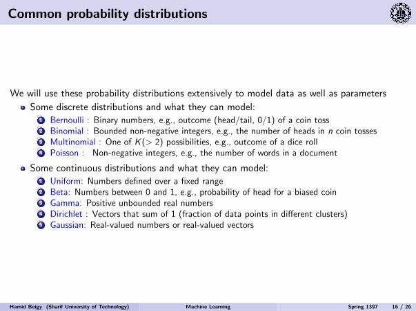
Common probability distributions

We will use these probability distributions extensively to model data as well as parameters

Some discrete distributions and what they can model:1 Bernoulli : Binary numbers, e.g., outcome (head/tail, 0/1) of a coin toss2 Binomial : Bounded non-negative integers, e.g., the number of heads in n coin tosses3 Multinomial : One of K (> 2) possibilities, e.g., outcome of a dice roll4 Poisson : Non-negative integers, e.g., the number of words in a document

Some continuous distributions and what they can model:1 Uniform: Numbers defined over a fixed range2 Beta: Numbers between 0 and 1, e.g., probability of head for a biased coin3 Gamma: Positive unbounded real numbers4 Dirichlet : Vectors that sum of 1 (fraction of data points in different clusters)5 Gaussian: Real-valued numbers or real-valued vectors


Outline

1 Probability

2 Random variables



5 Bayes theorem

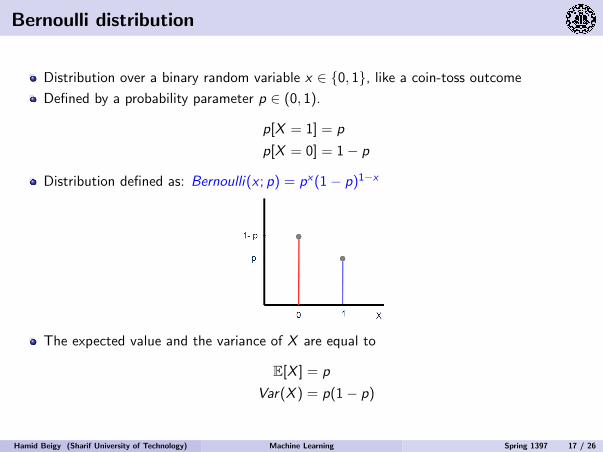
Bernoulli distribution

Distribution over a binary random variable x ∈ 0, 1, like a coin-toss outcome

Defined by a probability parameter p ∈ (0, 1).

p[X = 1] = p

p[X = 0] = 1− p

Distribution defined as: Bernoulli(x ; p) = px(1− p)1−x

Bernoulli Distribution

Distribution over a binary r.v. x 2 0, 1, like a coin-toss outcome

Defined by a probability parameter p 2 (0, 1)

P(x = 1) = p

Distribution defined as: Bernoulli(x ; p) = p

x(1 p)1x

Mean: E[x ] = p

Variance: var[x ] = p(1 p)


The expected value and the variance of X are equal to

E[X ] = p

Var(X ) = p(1− p)


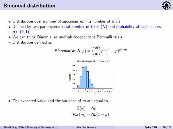
Binomial distribution

Distribution over number of successes m in a number of trials

Defined by two parameters: total number of trials (N) and probability of each successp ∈ (0, 1).

We can think Binomial as multiple independent Bernoulli trials

Distribution defined as

Binomial(m;N, p) =

(N

m

)pm(1− p)N−m

Binomial Distribution

Distribution over number of successes m (an r.v.) in a number of trials

Defined by two parameters: total number of trials (N) and probability ofeach success p 2 (0, 1)

Can think of Binomial as multiple independent Bernoulli trials

Distribution defined as

Binomial(m;N, p) =

N

m

p

m(1 p)Nm

Mean: E[m] = Np

Variance: var[m] = Np(1 p)


The expected value and the variance of m are equal to

E[m] = Np

Var(m) = Np(1− p)


Multinomial distribution

Consider a generalization of Bernoulli where the outcome of a random event is one of Kmutually exclusive and exhaustive states, each of which has a probability of occurring qiwhere

∑Ki=1 qi = 1.

Suppose that n such trials are made where outcome i occurred ni times with∑K

i=1 ni = n.

The joint distribution of n1, n2, . . . , nK is multinomial

P(n1, n2, . . . , nK ) = n!K∏i=1

qniini !


Outline

1 Probability

2 Random variables



5 Bayes theorem

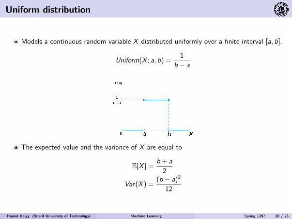
Uniform distribution

Models a continuous random variable X distributed uniformly over a finite interval [a, b].

Uniform(X ; a, b) =1

b − a

Uniform Distribution

Models a continuous r.v. x distributed uniformly over a finite interval [a, b]

Uniform(x ; a, b) =1

b a

Mean: E[x ] = (b+a)

2

Variance: var[x ] = (ba)

2

12


The expected value and the variance of X are equal to

E[X ] =b + a

2

Var(X ) =(b − a)2

12


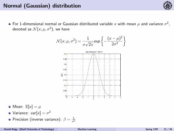
Normal (Gaussian) distribution

For 1-dimensional normal or Gaussian distributed variable x with mean µ and variance σ2,denoted as N (x ;µ, σ2), we have

N (x ;µ, σ2) =1

σ√2π

exp

−(x − µ)2

2σ2

Mean: E[x ] = µ

Variance: var [x ] = σ2

Precision (inverse variance): β = 1σ2


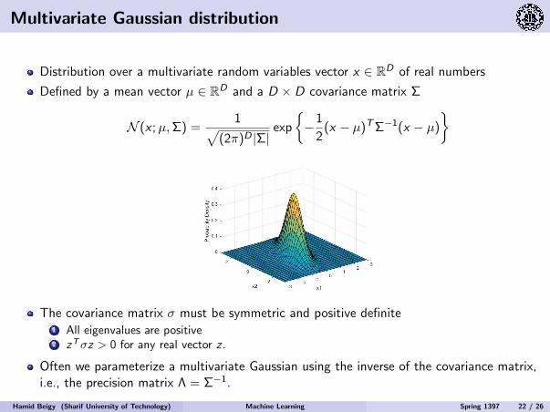
Multivariate Gaussian distribution

Distribution over a multivariate random variables vector x ∈ RD of real numbers

Defined by a mean vector µ ∈ RD and a D × D covariance matrix Σ

N (x ;µ,Σ) =1√

(2π)D |Σ|exp

−1

2(x − µ)TΣ−1(x − µ)

Multivariate Gaussian Distribution

Distribution over a multivariate r.v. vector 2 RD of real numbers

Defined by a mean vector µ 2 RD and a D D covariance matrix

N ( ;µ,) =1p

(2)D ||e

1

2

( µ)

>

1

( µ)

The covariance matrix must be symmetric and positive definite

All eigenvalues are positive

> > 0 for any real vector

Often we parameterize a multivariate Gaussian using the inverse of thecovariance matrix, i.e., the precision matrix =

1


The covariance matrix σ must be symmetric and positive definite1 All eigenvalues are positive2 zTσz > 0 for any real vector z .

Often we parameterize a multivariate Gaussian using the inverse of the covariance matrix,i.e., the precision matrix Λ = Σ−1.


Outline

1 Probability

2 Random variables



5 Bayes theorem


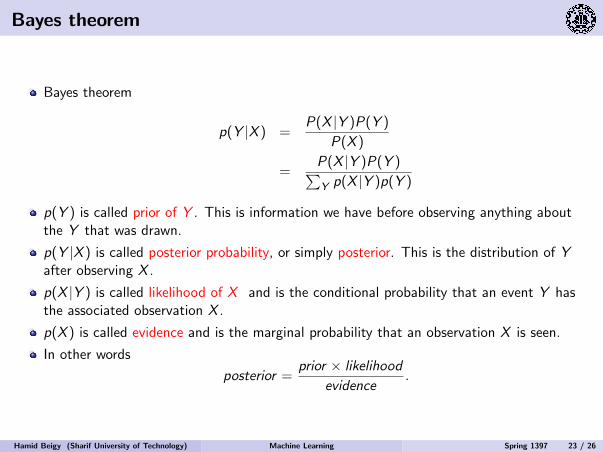
Bayes theorem

Bayes theorem

p(Y |X ) =P(X |Y )P(Y )

P(X )

=P(X |Y )P(Y )∑Y p(X |Y )p(Y )

p(Y ) is called prior of Y . This is information we have before observing anything aboutthe Y that was drawn.

p(Y |X ) is called posterior probability, or simply posterior. This is the distribution of Yafter observing X .

p(X |Y ) is called likelihood of X and is the conditional probability that an event Y hasthe associated observation X .

p(X ) is called evidence and is the marginal probability that an observation X is seen.

In other words

posterior =prior × likelihood

evidence.


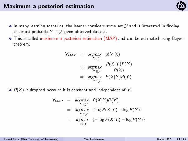
Maximum a posteriori estimation

In many learning scenarios, the learner considers some set Y and is interested in findingthe most probable Y ∈ Y given observed data X .

This is called maximum a posteriori estimation (MAP) and can be estimated using Bayestheorem.

YMAP = argmaxY∈Y

p(Y |X )

= argmaxY∈Y

P(X |Y )P(Y )

P(X )

= argmaxY∈Y

P(X |Y )P(Y )

P(X ) is dropped because it is constant and independent of Y .

YMAP = argmaxY∈Y

P(X |Y )P(Y )

= argmaxY∈Y

logP(X |Y ) + logP(Y )

= argminY∈Y

− logP(X |Y )− logP(Y )


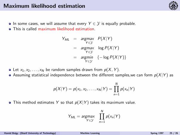
Maximum likelihood estimation

In some cases, we will assume that every Y ∈ Y is equally probable.This is called maximum likelihood estimation.

YML = argmaxY∈Y

P(X |Y )

= argmaxY∈Y

logP(X |Y )

= argminY∈Y

− logP(X |Y )

Let x1, x2, . . . , xN be random samples drawn from p(X ,Y ).Assuming statistical independence between the different samples,we can form p(X |Y ) as

p(X |Y ) = p(x1, x2, . . . , xN |Y ) =N∏

n=1

p(xn|Y )

This method estimates Y so that p(X |Y ) takes its maximum value.

YML = argmaxY∈Y

N∏n=1

p(xn|Y )


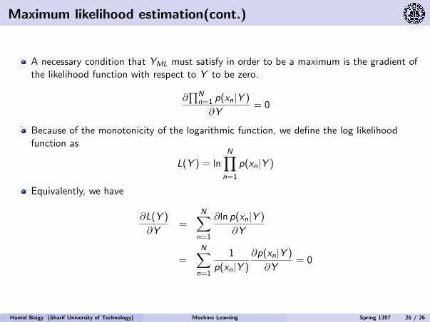
Maximum likelihood estimation(cont.)

A necessary condition that YML must satisfy in order to be a maximum is the gradient ofthe likelihood function with respect to Y to be zero.

∂∏N

n=1 p(xn|Y )

∂Y= 0

Because of the monotonicity of the logarithmic function, we define the log likelihoodfunction as

L(Y ) = lnN∏

n=1

p(xn|Y )

Equivalently, we have

∂L(Y )

∂Y=

N∑n=1

∂ln p(xn|Y )

∂Y

=N∑

n=1

1

p(xn|Y )

∂p(xn|Y )

∂Y= 0


machine learning - sharif university of...

Documents