machine learning techniques for gesture recognition carlos ... · machine learning techniques for...
TRANSCRIPT
Machine Learning Techniques for Gesture Recognition
Carlos Antonio Caceres
Thesis submitted to the faculty of the Virginia Polytechnic Institute and State University
in partial fulfillment of the requirements for the degree of
Master of Science
In
Mechanical Engineering
Alfred L. Wicks, Chair
John P. Bird
Craig A. Woolsey
September 9th
, 2014
Blacksburg, VA
Keywords: Gesture Recognition, Smart Prosthetic, Hidden Markov Model, Support
Vector Machines, Dynamic Time Warping
Machine Learning Techniques for Gesture Recognition
Carlos Antonio Caceres
ABSTRACT
Classification of human movement is a large field of interest to Human-Machine
Interface researchers. The reason for this lies in the large emphasis humans place on
gestures while communicating with each other and while interacting with machines. Such
gestures can be digitized in a number of ways, including both passive methods, such as
cameras, and active methods, such as wearable sensors. While passive methods might be
the ideal, they are not always feasible, especially when dealing in unstructured
environments. Instead, wearable sensors have gained interest as a method of gesture
classification, especially in the upper limbs. Lower arm movements are made up of a
combination of multiple electrical signals known as Motor Unit Action Potentials
(MUAPs). These signals can be recorded from surface electrodes placed on the surface of
the skin, and used for prosthetic control, sign language recognition, human machine
interface, and a myriad of other applications.
In order to move a step closer to these goal applications, this thesis compares
three different machine learning tools, which include Hidden Markov Models (HMMs),
Support Vector Machines (SVMs), and Dynamic Time Warping (DTW), to recognize a
number of different gestures classes. It further contrasts the applicability of these tools to
noisy data in the form of the Ninapro dataset, a benchmarking tool put forth by a
conglomerate of universities. Using this dataset as a basis, this work paves a path for the
analysis required to optimize each of the three classifiers. Ultimately, care is taken to
compare the three classifiers for their utility against noisy data, and a comparison is made
against classification results put forth by other researchers in the field.
The outcome of this work is 90+ % recognition of individual gestures from the
Ninapro dataset whilst using two of the three distinct classifiers. Comparison against
previous works by other researchers shows these results to outperform all other thus far.
Through further work with these tools, an end user might control a robotic or prosthetic
arm, or translate sign language, or perhaps simply interact with a computer.

iii
Dedication
For my family.

iv
Acknowledgements
I’d like to use these lines to thank all those people who helped get me to this
point. Graduate school has been an amazing journey, where I have learned more than I
could’ve hoped for, met some of the brightest and best people I know, and ultimately
grown as a person and an engineer.
Particular thanks go to my committee members, without whom the last two years
would have been a much more difficult path. First, Dr. Craig Woolsey, whose help and
kindness in my early days at Virginia Tech helped guide me towards the kind of research
I wanted to follow. Second, Dr. John Bird who has been a constant source of wisdom and
guidance during my time as a graduate student. And finally, my sincerest appreciation
and respect to Dr. Al Wicks. Without the opportunities and support of Dr. Wicks,
graduate school would have been a constant struggle. For these reasons and many more,
these three men have earned my lifelong respect and appreciation.
Finally, I must thank my parents, who have worked extremely hard since arriving
in this country, all for the benefit of their children.

v
Table of Contents
Dedication ...................................................................................................................................... iii
Acknowledgements ........................................................................................................................ iv
Table of Contents ............................................................................................................................ v
List of Figures .............................................................................................................................. viii
List of Tables .................................................................................................................................. x
Acronyms ........................................................................................................................................ x
1 Introduction .............................................................................................................................. 1
1.1 Background Problem ............................................................................................ 1
1.2 Proposed Solution ................................................................................................ 4
1.3 Thesis Structure .................................................................................................... 4
1.4 Summary .............................................................................................................. 5
2 Literature Review .................................................................................................................... 7
2.1 Chapter Summary ................................................................................................. 7
2.2 Previous Research ................................................................................................ 7
2.3 Summary ............................................................................................................ 11
3 Background Theory ............................................................................................................... 12
3.1 Chapter Summary ............................................................................................... 12
3.2 Electromyography .............................................................................................. 12
3.3 Physiology .......................................................................................................... 14
3.4 Machine Learning .............................................................................................. 15
3.4.1 Hidden Markov Models .............................................................................. 16
3.4.2 Dynamic Time Warping ............................................................................. 19
3.4.3 Support Vector Machine ............................................................................. 23
3.5 Summary ............................................................................................................ 24
4 Methods ................................................................................................................................. 26
4.1 Chapter Summary ............................................................................................... 26
4.2 Dataset ................................................................................................................ 26
4.3 Active Segments ................................................................................................. 29
vi
4.4 Feature Extraction .............................................................................................. 30
4.5 Feature Selection ................................................................................................ 33
4.6 Hidden Markov Models ..................................................................................... 36
4.6.1 Vector Discretization .................................................................................. 37
4.6.2 Model Setup ................................................................................................ 38
4.6.3 Left to Right vs. Ergodic Models ................................................................ 39
4.6.4 Effect of Increasing Vocabulary ................................................................. 39
4.6.5 Minimum Required Training Data.............................................................. 40
4.6.6 Optimized Model ........................................................................................ 40
4.7 Support Vector Machines ................................................................................... 42
4.7.1 Data Scaling ................................................................................................ 43
4.7.2 Kernel Test .................................................................................................. 44
4.7.3 Effect of Increasing Vocabulary ................................................................. 44
4.7.4 Minimum Required Training Data.............................................................. 44
4.7.5 Optimized Model ........................................................................................ 45
4.8 Dynamic Time Warping ..................................................................................... 45
4.8.1 Data Preparation.......................................................................................... 46
4.8.2 Threshold calculation .................................................................................. 46
4.8.3 Optimized Model ........................................................................................ 47
4.9 Summary ............................................................................................................ 47
5 Results.................................................................................................................................... 49
5.1 Chapter Summary ............................................................................................... 49
5.2 Optimal Data and Feature Representation ......................................................... 50
5.2.1 Feature Threshold ....................................................................................... 50
5.2.2 Number of frames ....................................................................................... 52
5.2.3 Filter method feature selection .................................................................... 53
5.2.4 Hidden Markov Model Wrapper ................................................................. 54
5.2.5 Support Vector Machine Wrapper .............................................................. 55
5.3 Dynamic Time Warping Results ........................................................................ 56
5.3.1 Number of Examples and Data Preparation Test ........................................ 56
5.3.2 Final Model ................................................................................................. 58
vii
5.3.3 Issues with Dynamic Time Warping Method ............................................. 60
5.4 Hidden Markov Model Results .......................................................................... 62
5.4.1 Model Setup ................................................................................................ 62
5.4.2 Left to Right vs. Ergodic Models ................................................................ 63
5.4.3 Effect of Increasing Vocabulary ................................................................. 64
5.4.4 Minimum Required Training Data.............................................................. 65
5.4.5 Final Feature Model .................................................................................... 66
5.4.6 Final SAX Model ........................................................................................ 69
5.5 SVM Results ...................................................................................................... 72
5.5.1 Kernel Test .................................................................................................. 73
5.5.2 Effect of Increasing Vocabulary ................................................................. 74
5.5.3 Minimum Required Training Data.............................................................. 75
5.5.4 Final SVM Model ....................................................................................... 75
5.6 Summary ............................................................................................................ 77
6 Conclusions............................................................................................................................ 78
6.1 Chapter Summary ............................................................................................... 78
6.2 Previous Ninapro Results ................................................................................... 78
6.3 Thesis Results ..................................................................................................... 79
6.4 Achievement....................................................................................................... 81
6.5 Future work ........................................................................................................ 82
6.6 Summary ............................................................................................................ 83
References ..................................................................................................................................... 84
Appendix A: Gesture Dictionary .................................................................................................. 89
Appendix B: EMG Features.......................................................................................................... 91
viii
List of Figures
Figure 1: ASL Hand Signs [1] ............................................................................................ 2
Figure 2: SWAT Team Hand Signs [2] .............................................................................. 2
Figure 3: Control Strategy for Smart Prosthetics [8] .......................................................... 3
Figure 4: The Motor Unit [26] .......................................................................................... 12
Figure 5: Motorneuron's EMG Signal Generation [25] .................................................... 13
Figure 6: Forearm Muscle Groups [27] ............................................................................ 15
Figure 7: HMM Topologies, left to right (top) and ergodic (bottom) [17] ....................... 17
Figure 8: DTW Method [31] ............................................................................................. 20
Figure 9: DTW Optimal Warping Path [31] ..................................................................... 21
Figure 10: DTW Classification Process [17] .................................................................... 22
Figure 11: SVM Margin [17] ............................................................................................ 23
Figure 12: Sensor Setup [11] ............................................................................................ 27
Figure 13: Experiment Setup [12]..................................................................................... 27
Figure 14: FFT of Gesture Waveform .............................................................................. 29
Figure 15: EMG Active Segment[24] ............................................................................... 30
Figure 16: Filter Feature Selection Approach [39] ........................................................... 34
Figure 17: Wrapper Feature Selection Approach [39] ...................................................... 35
Figure 18: SAX Discretization [17] .................................................................................. 38
Figure 19: Log Likelihood / Probability Correspondence ................................................ 42
Figure 20: One-Against-All Approach to SVM Training [37] ......................................... 43
Figure 21: Confusion Matrix Example ............................................................................. 50
Figure 22: SVM Wrapper Threshold Calculation ............................................................. 51
Figure 23: Signal to Noise Difference Threshold Calculation .......................................... 52
Figure 24: SVM Wrapper Number of Frames Calculation ............................................... 53
Figure 25: Filter Based Feature Ranking .......................................................................... 54
Figure 26: DTW 8 Class Confusion Matrix ...................................................................... 58
Figure 27: DTW 8 Class Precision and Recall ................................................................. 58
Figure 28: DTW 18 Class Confusion Matrix .................................................................... 59
Figure 29: DTW 18 Class Precision and Recall ............................................................... 59
ix
Figure 30: Gesture 2 Iteration Distances from Templates ................................................ 61
Figure 31: Example Misclassification Distances .............................................................. 61
Figure 32: HMM States and Symbols Test ....................................................................... 63
Figure 33: HMM Number of Skipped States Test ............................................................ 64
Figure 34: HMM Accuracy Over Number of Classes ...................................................... 65
Figure 35: HMM Minimum Amount of Training Data .................................................... 66
Figure 36: HMM Recall and Precision Test ..................................................................... 67
Figure 37: HMM Optimized Results ................................................................................ 68
Figure 38: HMM Sub-Optimal Test ................................................................................. 68
Figure 39: HMM Gesture Separability ............................................................................. 68
Figure 40: Movement ID and Descriptions [12] ............................................................... 69
Figure 41: SAX Discretization Confusion Matrix ............................................................ 70
Figure 42: SAX Discretized Recall and Precision ............................................................ 70
Figure 43: SAX Individual User Results (Overfitting) ..................................................... 71
Figure 44: SAX General Test (Underfitting) .................................................................... 72
Figure 45: Linear Kernel Average Cross Validation Ratio .............................................. 73
Figure 46: RBF Kernel Parameter Search ........................................................................ 74
Figure 47: SVM Performance vs. Number of Classes ...................................................... 74
Figure 48: SVM Learning Curve ...................................................................................... 75
Figure 49: SVM Optimized Average Cross Validation Ratio Results ............................. 76
Figure 50: SVM Optimized Recall and Precision ............................................................. 77
Figure 51: SVM Time Complexity ................................................................................... 80
Figure 52: HMM Time Complexity .................................................................................. 80
Figure 53: DTW Time Complexity................................................................................... 80
Figure 54: Overall Classifier Performance ....................................................................... 81

x
List of Tables
Table 1: HMM Wrapper Feature Subset Scores ............................................................... 55
Table 2: SVM Wrapper Feature Subset Scores ................................................................ 55
Table 3: SAX vs. Down Sampling DTW.......................................................................... 57
Table 4: Ninapro Classification Results ........................................................................... 78
Acronyms
ACVR Average Cross Validation Ratio
ANN Artificial Neural Network
ANOVA Analysis of Variance
APR Average Precision Ratio
ARR Average Recall Ratio
ASL American Sign Language
DP Dynamic Programming
DTW Dynamic Time Warping
ECG Electrocardiography
EMG Electromyography
HMM Hidden Markov Model
KNN K-Nearest Neighbors
IMU Inertial Measurement Unit
MAP Muscle Action Potential
MN Motor Neuron
MU Motor Unit
MUAP Motor Unit Action Potential
RBF Radial Basis Function
SAX Symbolic Aggregate Approximation
SFS Sequential Forward Selection
SFFS Sequential Forward Floating Selection
SVM Support Vector Machine

1
1 Introduction
1.1 Background Problem
There is a current trend in technology to expand the use of custom wearable
devices. Such gadgets range from portable phones to smart watches and recently the
onset of custom smart prosthetics. It is precisely the expansion of these technologies
which has propelled forward the study of machine learning oriented activity recognition.
In this context, machine learning is the use of computational tools to extract and decipher
a pattern within data. The recognition of these patterns is then molded towards an end
goal of use, such as recognizing a human action, and through it, a person’s intent.
The work that follows tries to aid in the study of this field by making a
comparison of the implementation and the optimization of different machine learning
methods for gesture recognition. Though the end goal of gesture recognition and
classification might seem better suited for a tool such as cameras, which would avoid the
hindrance of having electronics attached to the body, this work begins with the
assumption that alternative approaches to gesture recognition are not feasible in many
situations. For instance, cameras require very structured environments to capture data in a
way that could be used for a computer system and gesture recognition. Lighting becomes
an issue, as does the possible use of such a system in spaces void of a proper camera
setup. Instead, this work makes the assumption that there are many more benefits to a
wearable device.
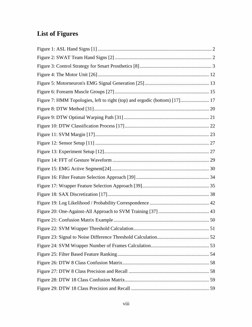
Such a device might eventually be used in multiple contexts where gesture
recognition is an option. For instance, much research has gone into using such a system
for sign language translation into speech and vice versa. This capacity would allow for
better communication between people, and would be based on the already gesture defined
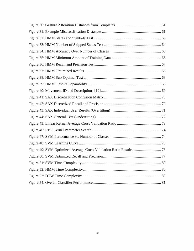
American Sign Language dictionary shown in Figure 1. Another use of a gesture
recognition system lies in swat team and military operations which often make the use of
tactical hand signs. These signs, as shown in Figure 2, supplement speech where
concealment is needed such as in tactical operations, or where high noise levels
overpower the voice, such as landing zones. Finally, the last example which will be
2
offered also covers the principal motivation of this work, that of smart prosthetics for
upper limb amputees.
Figure 1: ASL Hand Signs, J. Strickland, “The Sign Language Alphabet,” How Stuff Works, 2007. [Online]. Available:
http://people.howstuffworks.com/sign-language2.htm.
Used under fair use, 2014.
Figure 2: SWAT Team Hand Signs, S. A. R. Tidwell S. Karlaputi, R. Akl, K. Kavi and D. Struble, “Evaluating the
feasibility of EMG and bend sensors for classifying hand gestures,” in Proceedings of the International
Conference on Multimedia and Human Computer Interaction (MHCI-13), 2013.
Used under fair use, 2014.
3
In the USA, there are an estimated 50,000 new amputations every year [3]. Of
those, roughly 10,000 are amputations of the upper extremities [4]. Though passive
prosthetics have been the most popular option thus far, electromyography (EMG)
controlled active replacements are quickly gaining traction in the medical community.
This is due to the increased control and quality of life such an option offers.
After an amputation, forearm muscles remain largely intact [5]. Evidence even
subjects that EMG signals from amputees are very similar to those generated by intact
subjects [6]. For instance, even though intrinsic muscles, which control many degrees of
freedom, are no longer present for below the elbow amputees, it is still possible to control
certain degrees of freedom such as hand flexion and extension through extrinsic forearm
muscles [7]. This is why the following work, like many such works in this field, makes
the use of intact subjects which are more readily available for testing proof of concept
trials. The methods which culminates from these tests can then be translated to amputees
with little loss of functionality or generalization.
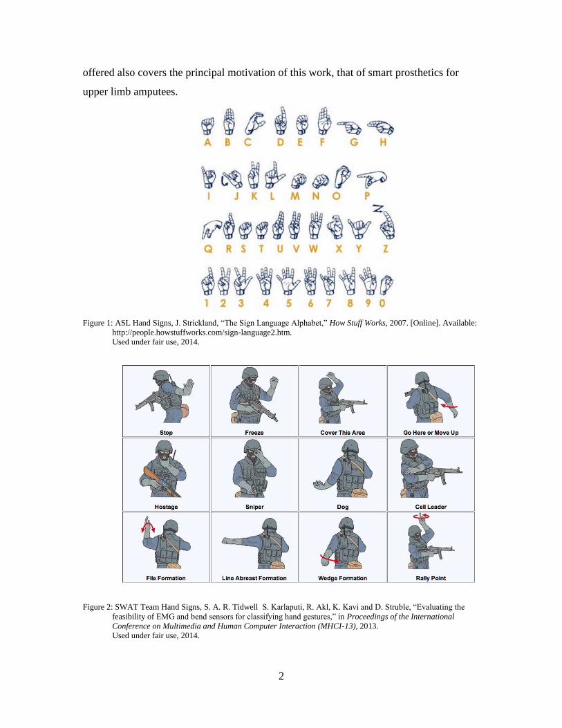
Using these assumptions and approach, multiple systems have been developed
which seek to offer multi-functional prosthetic control. For example, Figure 3 shows a
system overview of the work done by Dr. Marko Vuskovic which demonstrates the
process many researchers seek for prosthetic control: EMG collection, feature extraction
and classification, force and movement mapping, and finally control [8].
Figure 3: Control Strategy for Smart Prosthetics, A. Esquenazi, “Amputation rehabilitation and prosthetic restoration.
From surgery to community reintegration,” Disabil. Rehabil., vol. 26, no. 14–15, pp. 831–836, Jan. 2004.
Used under fair use, 2014.

4
1.2 Proposed Solution
Gesture recognition is an old problem with many proposed solutions. Even though
the Holy Grail of gesture recognition is to simulate human vision and use passive
systems, such as cameras, this technique suffers from major drawbacks. For instance,
finger occlusion can be very high depending on point of view. Because of this issue,
multiple gestures can look exactly the same to a passive camera [9]. Still many
researchers have taken the vision based approach.
In this work, EMG based gesture recognition is proposed in order to alleviate
some of the issues of vision based systems. With this technique, it is possible to avoid the
point of view issue already mentioned, as well as other issues such as the required camera
infrastructure, the necessity for a clear line of sight, any need for constant lighting,
resolution and range problems, and even frame rate [10]. In order to do EMG gesture
classification, this thesis compares three different machine learning tools, Hidden Markov
Models, Support Vector Machines, and Dynamic Time Warping, to recognize different
gestures classes. It further contrasts the applicability of these tools to noisy data in the
form of the Ninapro dataset, a benchmarking tool put forth by a conglomerate of
universities [11], [12]. Using this dataset as a basis, this work paves a path for the
analysis required to optimize each of the three classifiers. Ultimately, care is taken to
compare the three classifiers for their utility against noisy data, and a comparison is made
against classification results put forth by other researchers in the field.
1.3 Thesis Structure
This thesis will deal with the design, analysis, and optimization of machine
learning algorithms for use in gesture recognition. This work was motivated by the desire
to apply machine learning tools to the improvement of machine human interface through
electromyography. Such interfaces are quickly gaining traction in industry, with multiple
recent startups gaining popularity [13]. Within this field, this thesis’ achievements will
concentrate on using such a system for smart prosthetics which might aid amputees.
As will be seen, much of this work deals with the optimization of multiple gesture
classifiers through experimentation. There is also a large emphasis on the comparison of
the methods chosen and how they might be suited for different kinds of data. Ultimately,

5
a choice is made based on repeated experiments on the classifiers and the EMG Ninapro
database. Also, as will be seen, even though not a real time design, the accuracies
achieved in this work are on par with current state of the art research systems, and could
be extended to perform online recognition.
The rest of this thesis is structured as follows. Chapter 2 offers a variety of
previous works in the field, specializing in gesture recognition for prosthetic control.
Chapter 3 will cover the background theory behind the major blocks of this work,
beginning with electromyography, or the use of electrodes to measure muscle electrical
potential; then upper limb physiology will be reviewed as it pertains to arm gesture
recognition and prosthetic control. Finally, the three learning classifiers will be covered
in order to give the reader a basic understanding of how they operate.
Following the background theory, chapter 4 will cover the methods used in this
work in detail. This will include the datasets used for learning as well as the code used.
Most importantly, chapter 4 also goes on to setup a number of experiments which were
conducted in the search for classifier optimization.
Chapter 5 goes on to cover the results of the analysis. First, results for the data
representation experiments are presented. These results show how the Ninapro dataset
was represented for each of the three learning methods. Secondly, each of the three
classifiers is studied in detail through their individual experiments.
Finally, chapter 6 will offer concluding remarks discussing the ultimate outcomes
of the three gesture classifiers including their performance, the final achievements as the
author sees them, and potential future work which might branch off from this thesis.
1.4 Summary
The current chapter has worked to setup the basic problem that this thesis tries to
tackle. Through reading the background problem and proposed solution sections, the
author hopes that the reader gets an appreciation for the realm this work fits into, and
where it can be applied. Furthermore, this chapter has also worked to preview the
remainder of this thesis and give the reader a roadmap for what is to come.
Now that the groundwork has been laid for the problem at hand, the following
chapter will present a few of the numerous works available in the gesture recognition

6
community. Through these examples, the reader should get a sense of the diversity within
this up and coming field, as well as where some of the ideas in this thesis come from.
7
2 Literature Review
2.1 Chapter Summary
Chapter 2 of this thesis will contribute two important aspects to setting up this
work. First, it will concentrate on machine learning methods as they relate to gesture
recognition. Second, certain works will be reviewed which although outside the scope of
the current work, nonetheless show future development which might spin off from this
work. On the first topic, while there are too many such works to cover them all, the
following few have been chosen as those with the greatest effect on this work. In
investigating these, the reader should get a sense of how popular and diverse machine
learning gesture recognition is.
2.2 Previous Research
There are a lot of works which concentrate on wearable devices for gesture
recognition. These works range in scope from small projects by undergraduate
engineering students, to Master’s Thesis, and much further into million dollar projects
such as that conducted by NASA’s JPL. What follows are a few such works that
contributed to this thesis, either by offering simple guidelines, explanations and
examples, or even aiding in defining the scope.
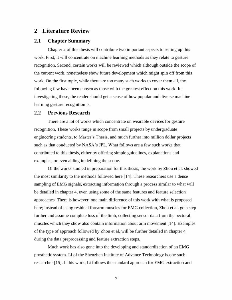
Of the works studied in preparation for this thesis, the work by Zhou et al. showed
the most similarity to the methods followed here [14]. These researchers use a dense
sampling of EMG signals, extracting information through a process similar to what will
be detailed in chapter 4, even using some of the same features and feature selection
approaches. There is however, one main difference of this work with what is proposed
here; instead of using residual forearm muscles for EMG collection, Zhou et al. go a step
further and assume complete loss of the limb, collecting sensor data from the pectoral
muscles which they show also contain information about arm movement [14]. Examples
of the type of approach followed by Zhou et al. will be further detailed in chapter 4
during the data preprocessing and feature extraction steps.
Much work has also gone into the developing and standardization of an EMG
prosthetic system. Li of the Shenzhen Institute of Advance Technology is one such
researcher [15]. In his work, Li follows the standard approach for EMG extraction and
8
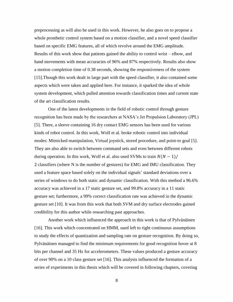
preprocessing as will also be used in this work. However, he also goes on to propose a
whole prosthetic control system based on a motion classifier, and a novel speed classifier
based on specific EMG features, all of which revolve around the EMG amplitude.
Results of this work show that patients gained the ability to control wrist – elbow, and
hand movements with mean accuracies of 96% and 87% respectively. Results also show
a motion completion time of 0.38 seconds, showing the responsiveness of the system
[15].Though this work dealt in large part with the speed classifier, it also contained some
aspects which were taken and applied here. For instance, it sparked the idea of whole
system development, which pulled attention towards classification times and current state
of the art classification results.
One of the latest developments in the field of robotic control through gesture
recognition has been made by the researchers at NASA’s Jet Propulsion Laboratory (JPL)
[5]. There, a sleeve containing 16 dry contact EMG sensors has been used for various
kinds of robot control. In this work, Wolf et al. broke robotic control into individual
modes: Mimicked manipulation, Virtual joystick, stored procedure, and point-to goal [5].
They are also able to switch between command sets and even between different robots
during operation. In this work, Wolf et al. also used SVMs to train
classifiers (where N is the number of gestures) for EMG and IMU classification. They
used a feature space based solely on the individual signals’ standard deviations over a
series of windows to do both static and dynamic classification. With this method a 96.6%
accuracy was achieved in a 17 static gesture set, and 99.8% accuracy in a 11 static
gesture set; furthermore, a 99% correct classification rate was achieved in the dynamic
gesture set [10]. It was from this work that both SVM and dry surface electrodes gained
credibility for this author while researching past approaches.
Another work which influenced the approach in this work is that of Pylvänäinen
[16]. This work which concentrated on HMM, used left to right continuous assumptions
to study the effects of quantization and sampling rate on gesture recognition. By doing so,
Pylvänäinen managed to find the minimum requirements for good recognition hover at 8
bits per channel and 35 Hz for accelerometers. These values produced a gesture accuracy
of over 90% on a 10 class gesture set [16]. This analysis influenced the formation of a
series of experiments in this thesis which will be covered in following chapters, covering
9
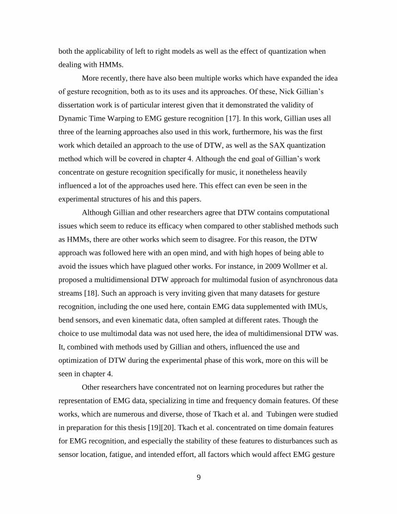
both the applicability of left to right models as well as the effect of quantization when
dealing with HMMs.
More recently, there have also been multiple works which have expanded the idea
of gesture recognition, both as to its uses and its approaches. Of these, Nick Gillian’s
dissertation work is of particular interest given that it demonstrated the validity of
Dynamic Time Warping to EMG gesture recognition [17]. In this work, Gillian uses all
three of the learning approaches also used in this work, furthermore, his was the first
work which detailed an approach to the use of DTW, as well as the SAX quantization
method which will be covered in chapter 4. Although the end goal of Gillian’s work
concentrate on gesture recognition specifically for music, it nonetheless heavily
influenced a lot of the approaches used here. This effect can even be seen in the
experimental structures of his and this papers.
Although Gillian and other researchers agree that DTW contains computational
issues which seem to reduce its efficacy when compared to other stablished methods such
as HMMs, there are other works which seem to disagree. For this reason, the DTW
approach was followed here with an open mind, and with high hopes of being able to
avoid the issues which have plagued other works. For instance, in 2009 Wollmer et al.
proposed a multidimensional DTW approach for multimodal fusion of asynchronous data
streams [18]. Such an approach is very inviting given that many datasets for gesture
recognition, including the one used here, contain EMG data supplemented with IMUs,
bend sensors, and even kinematic data, often sampled at different rates. Though the
choice to use multimodal data was not used here, the idea of multidimensional DTW was.
It, combined with methods used by Gillian and others, influenced the use and
optimization of DTW during the experimental phase of this work, more on this will be
seen in chapter 4.
Other researchers have concentrated not on learning procedures but rather the
representation of EMG data, specializing in time and frequency domain features. Of these
works, which are numerous and diverse, those of Tkach et al. and Tubingen were studied
in preparation for this thesis [19][20]. Tkach et al. concentrated on time domain features
for EMG recognition, and especially the stability of these features to disturbances such as
sensor location, fatigue, and intended effort, all factors which would affect EMG gesture
10
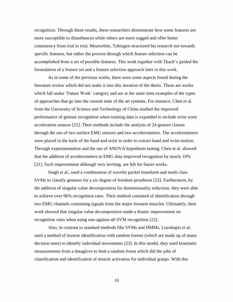
recognition. Through these results, these researchers demonstrate how some features are
more susceptible to disturbances while others are more rugged and offer better
consistency from trial to trial. Meanwhile, Tubingen structured his research not towards
specific features, but rather the process through which feature selection can be
accomplished from a set of possible features. This work together with Tkach’s guided the
formulation of a feature set and a feature selection approach later in this work.
As in some of the previous works, there were some aspects found during the
literature review which did not make it into this iteration of the thesis. These are works
which fall under ‘Future Work’ category and are at the same time examples of the types
of approaches that go into the current state of the art systems. For instance, Chen et al.
from the University of Science and Technology of China studied the improved
performance of gesture recognition when training data is expanded to include wrist worn
acceleration sensors [21]. Their methods include the analysis of 24 gesture classes
through the use of two surface EMG sensors and two accelerometers. The accelerometers
were placed in the back of the hand and wrist in order to extract hand and wrist motion.
Through experimentation and the use of ANOVA hypothesis testing, Chen et al. showed
that the addition of accelerometers to EMG data improved recognition by nearly 10%
[21]. Such improvement although very inviting, are left for future works.
Singh et al., used a combination of wavelet packet transform and multi class
SVMs to classify gestures for a six degree of freedom prosthesis [22]. Furthermore, by
the addition of singular value decomposition for dimensionality reduction, they were able
to achieve over 96% recognition rates. Their method consisted of identification through
two EMG channels containing signals from the major forearm muscles. Ultimately, their
work showed that singular value decomposition made a drastic improvement on
recognition rates when using one-against-all SVM recognition [22].
Also, in contrast to standard methods like SVMs and HMMs, Liarokapis et al.
used a method of inverse identification with random forests (which are made up of many
decision trees) to identify individual movements [23]. In this model, they used kinematic
measurements from a dataglove to feed a random forest which did the jobs of
classification and identification of muscle activation for individual grasps. With this
11
approach, Liarokapis et al. found improved results when compared to other classical
methods such as SVM and Artificial Neural Networks (ANN) [23].
And finally, Zhang et al, used a combination of EMG and accelerometers to
classify gestures from forearm sensors [24]. In their work they also used decision tree
classifiers, which included a HMM classifier as its last level. With this approach, they
achieved gesture recognition accuracy in the range of 95%-100% [24].
As can be seen from this brief overview, the works in gesture recognition are
broad and very distinct in their approaches. Many such works were studied and parts of
them borrowed for this work. Also, as was already mentioned, possible future work
following this thesis would further explore these works and seek to incorporate and test
more of their approaches.
2.3 Summary
Chapter 2 has emphasized previous works which have helped form and guide
prosthetic control. Through these few examples, the reader should get a sense that the
machine learning field, as it is applied to gesture recognition, is ample and diverse, with
much room for growth and experimentation.
These works and many more, were used in defining the methods which will be
covered in the following chapter. These methods were the result of research into previous
works combined with trial and error on the part of the author. With this in mind, the
following chapter will begin to dissect the background theory necessary for
understanding the approaches presented here.

12
3 Background Theory
3.1 Chapter Summary
This chapter will give a theoretical background on the major topics of this thesis.
In so doing, it will cover EMG signals and their relation to the human forearm
physiology, as well as machine learning techniques used to make sense and classify hand
gestures for use with active prosthesis.
What follows is a brief background on the major topics of this work, beginning
with EMG signals, their nature, and usefulness. Second, the physiology of the forearm
will be investigated in relation to the independent muscles that might be of interest when
it comes to gesture recognition. Finally, three machine learning tools will be described
and presented in the context of gestures recognition.
3.2 Electromyography
Electrodes are commonly used in the medical community to measure muscle
activation in relation to a patient’s health. Electrodes do this by measuring the electrical
activity of firing motor units (MU). An MU is made up of two parts, an alpha-moto
neurons (α- MNs) which transmit commands from the central nervous system to a
muscle, and the muscles which the α-MNs innervate [see Figure 4] [25].
Figure 4: The Motor Unit, N. Shapiro, “Motor Unit Recruitment Strategies During Deep Muscle Pain,” The alchemist.
[Online]. Available: http://natchem.wordpress.com/2009/11/23/motor-unit-recruitment-strategies-during-deep-
muscle-pain/.
Used under fair use, 2014.
Another important aspect of surface electrode, especially when compared to
needle electrodes, is the fact that these sensor covers a finite area over a patient’s skin.
13
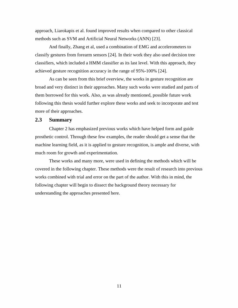
The effect of this, which can be seen in Figure 5, collects a mixture of various motor unit
action potentials (MUAPs) into a single sensor output.
Figure 5: Motorneuron's EMG Signal Generation, G. A. Garcia, R. Okuno, and K. Azakawa, “A decomposition
algorithm for surface electrode-array electromyogram,” Eng. Med. Biol. Mag. IEEE, vol. 24, no. 4, pp. 63–72,
2005.
Used under fair use, 2014.
The combination of multiple MUAPs is called a Compound Muscle Action
Potential (MAP); this is the signal captured by surface EMG sensors and lies in the range
of 50µV – 30mV and 7-200 Hz [2] [4].
As useful as EMG signals may be, they are not without issues. Compared to other bio
signals, EMG are susceptible to more types of noise that hinder proper signal processing.
For instance, EMG signals are plagued by equipment noise, electromagnetic radiation
from nearby sources, motion artifacts, in the range of 0 -15 Hz caused by the patient’s
movement, and even signal epenthesis as different MUAPs interact [27] [28]. The
following are a number of other factors which can affect EMG signals and cause both
issues as well as differentiate EMG on a per user basis [29]:
Muscle anatomy which includes the number, size, and distribution of motor units.
Muscle physiology which covers whether a specific muscle has undergone
training, is affected by a disorder or is undergoing fatigue.
Nerve factors such as nerve disorders.

14
Contraction level resulting from the intended applied force from subject to
subject.
Artifacts such as the already mentioned movement artefact, or others such as
muscle crosstalk and ECG interference.
Recording noise from recording machinery, electrodes, and even testing location.
3.3 Physiology
In terms of gesture recognition, EMG sensors capture an array of signals from
forearm muscles which correspond to different muscles associated with hand and wrist
movement. These signals are a mixture of various muscles and their corresponding motor
activations; although, machine learning (which we will look at more closely in following
sections) can decipher the pattern in these signals as a background step for classification,
it is still beneficial to try and understand how the muscle groups interact for specific
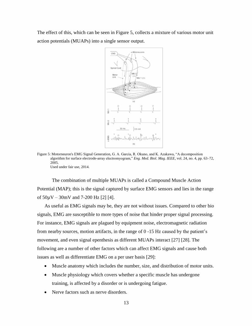
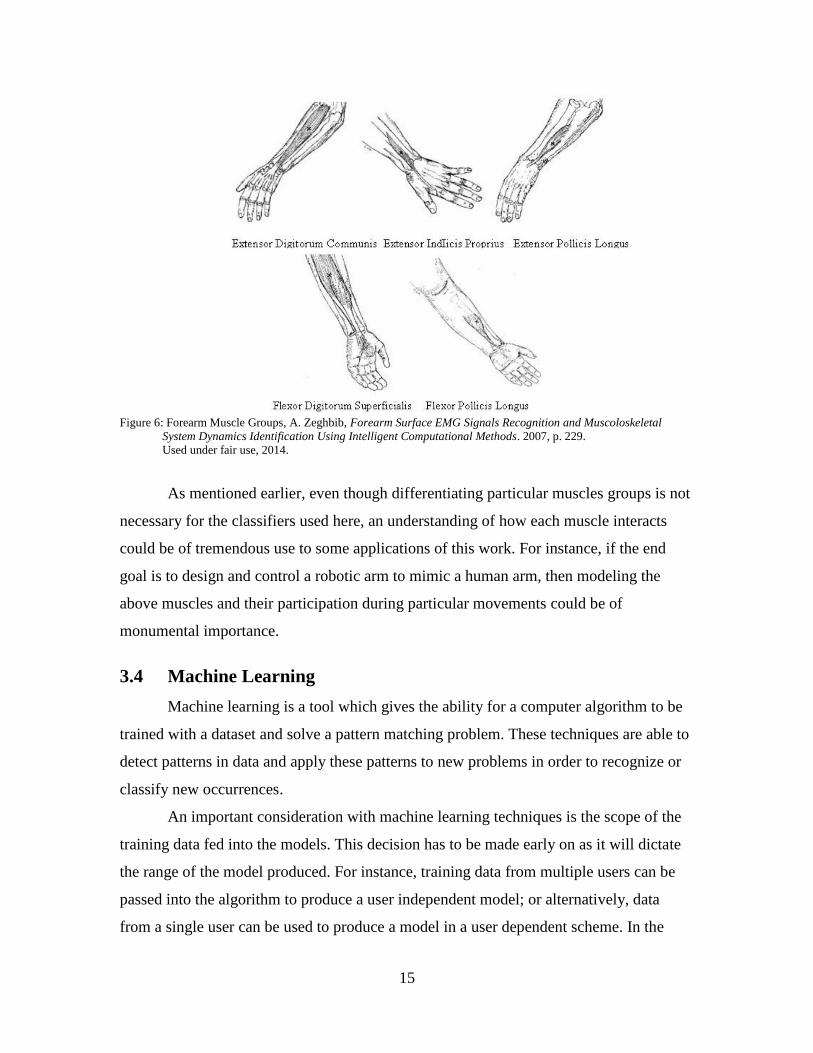
movements before undertaking a gesture classification project. There are three main hand
gesture activation methods and corresponding muscle groups [See Figure 6] we are
concern with, these are [27] :
1. Finger flexion
a. Flexor-digitorum-profundus
b. Flexordigitorum-
c. supercialis
d. Flexor-polcis-longus
2. Finger Extension
a. Extensor-digitorum
b. Extensor-indicis
c. Extensor-digiti-minimi
3. Thumb Extension
a. Extensor-pollicis-longus
b. Extensor-pollicis-brevis
15
Figure 6: Forearm Muscle Groups, A. Zeghbib, Forearm Surface EMG Signals Recognition and Muscoloskeletal
System Dynamics Identification Using Intelligent Computational Methods. 2007, p. 229.
Used under fair use, 2014.
As mentioned earlier, even though differentiating particular muscles groups is not
necessary for the classifiers used here, an understanding of how each muscle interacts
could be of tremendous use to some applications of this work. For instance, if the end
goal is to design and control a robotic arm to mimic a human arm, then modeling the
above muscles and their participation during particular movements could be of
monumental importance.
3.4 Machine Learning
Machine learning is a tool which gives the ability for a computer algorithm to be
trained with a dataset and solve a pattern matching problem. These techniques are able to
detect patterns in data and apply these patterns to new problems in order to recognize or
classify new occurrences.
An important consideration with machine learning techniques is the scope of the
training data fed into the models. This decision has to be made early on as it will dictate
the range of the model produced. For instance, training data from multiple users can be
passed into the algorithm to produce a user independent model; or alternatively, data
from a single user can be used to produce a model in a user dependent scheme. In the
16
case of EMG based gesture recognition, it has been found that individual gestures have
high variances and standard deviations. This fact implies that each person performing the
same gesture has their own unique gesture performing style [2]. Still, even though this
seems to imply that a user dependent model is necessary, this work will test this
assumption while also weighing the need for proper amounts of training data.
3.4.1 Hidden Markov Models
Hidden Markov Models (HMM) are a well-known tool for sequence recognition.
In the past they gained much popularity in the field of speech recognition due to their
intrinsic temporal capacity. HMMs can estimate both the probability of an observation
given a state, as well as the probability of an entire observation sequence occurring given
a model [17]. Thus, given N number of models (one for each gesture), HMMs can give us
the maximum likelihood of a gesture class taking place from a set of observations (EMG
recordings).
There are certain important parameters to consider when working with HMMs.
For instance, the models are created based on a feature space which has to be first
extracted from the data. As such, the computational complexity of the HMM recognition
is linearly dependent on the number of dimensions in the feature vector [16]; this means
that care must be taken when discretizing the EMG recordings. It has also been found that
for speech as well as gesture recognition, a left to right HMM offers the best accuracy
[16]. A left to right model implies a system in which the model’s states have to always
move in an ascending pattern. This contrasts the alternative approach in which all the
model’s states are inter-connected [See Figure 7] [17]. This is an important consideration
due to the computational complexity that comes from operating on a sparse vs. a dense
matrix.
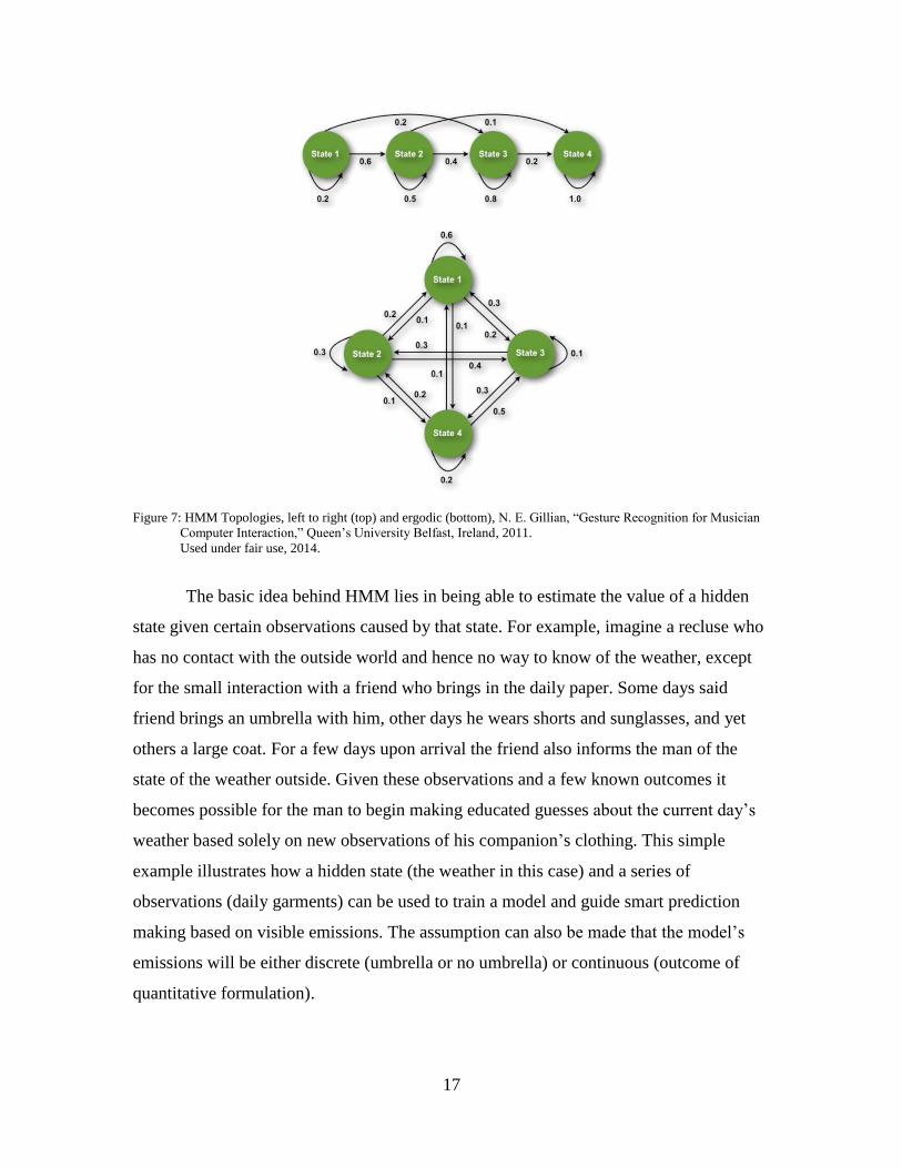
17
Figure 7: HMM Topologies, left to right (top) and ergodic (bottom), N. E. Gillian, “Gesture Recognition for Musician
Computer Interaction,” Queen’s University Belfast, Ireland, 2011.
Used under fair use, 2014.
The basic idea behind HMM lies in being able to estimate the value of a hidden
state given certain observations caused by that state. For example, imagine a recluse who
has no contact with the outside world and hence no way to know of the weather, except
for the small interaction with a friend who brings in the daily paper. Some days said
friend brings an umbrella with him, other days he wears shorts and sunglasses, and yet
others a large coat. For a few days upon arrival the friend also informs the man of the
state of the weather outside. Given these observations and a few known outcomes it
becomes possible for the man to begin making educated guesses about the current day’s
weather based solely on new observations of his companion’s clothing. This simple
example illustrates how a hidden state (the weather in this case) and a series of
observations (daily garments) can be used to train a model and guide smart prediction
making based on visible emissions. The assumption can also be made that the model’s
emissions will be either discrete (umbrella or no umbrella) or continuous (outcome of
quantitative formulation).
18
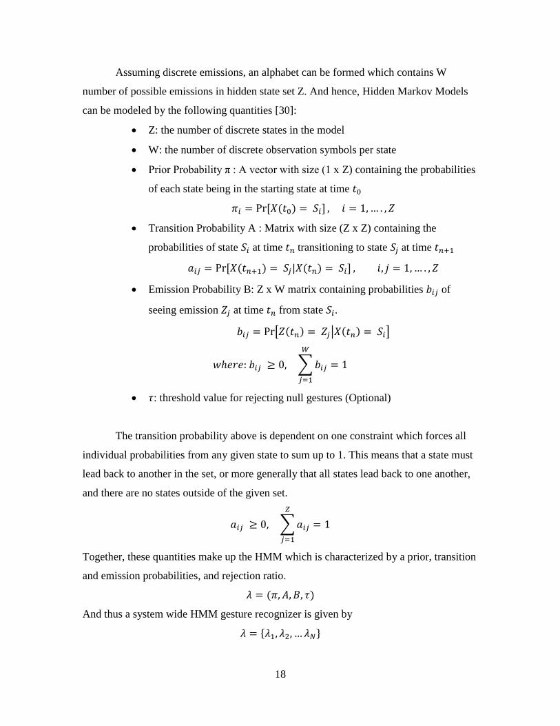
Assuming discrete emissions, an alphabet can be formed which contains W
number of possible emissions in hidden state set Z. And hence, Hidden Markov Models
can be modeled by the following quantities [30]:
Z: the number of discrete states in the model
W: the number of discrete observation symbols per state
Prior Probability π : A vector with size (1 x Z) containing the probabilities
of each state being in the starting state at time
Transition Probability A : Matrix with size (Z x Z) containing the
probabilities of state at time transitioning to state at time
Emission Probability B: Z x W matrix containing probabilities of
seeing emission at time from state .
[ | ]
∑
: threshold value for rejecting null gestures (Optional)
The transition probability above is dependent on one constraint which forces all
individual probabilities from any given state to sum up to 1. This means that a state must
lead back to another in the set, or more generally that all states lead back to one another,
and there are no states outside of the given set.
∑
Together, these quantities make up the HMM which is characterized by a prior, transition
and emission probabilities, and rejection ratio.
And thus a system wide HMM gesture recognizer is given by
{ }
19
Now that a base understanding of what a HMM is has been established, one can
begin to understand what a HMM can do. There are three basic problems to solve when
dealing with HMM:
1. Given a set of observations O, and a model , how is , the
probability of the observation sequence given the model, computed?
2. Given a set of observations O, and a model , how is a corresponding state
sequence S computed which best explains the observations.
3. Given an observation sequence O, how can the model parameters be
optimized to calculate the model .
For the problem of gesture recognition, problems 1 and 3 are the most important
as they cover training the model (problem 3), and recognition (problem 1). These two
problems can be solved by the Baum-Welch (training), and Forward-Backward
(recognition) algorithms. Looking at the details of these algorithms is beyond the scope
of this thesis; for more details of the specific mathematical relations please see Nick
Gillian’s dissertation on gesture recognition for music interfaces [17].
In the case of a gesture recognition system, each gesture model can be trained
with multiple observation sequences for more robust recognition. This is done by
calculating a model for each observation and combining them as:
∏ ( | ) .
Furthermore, a new observation sequence representing a gesture can be classified using
the maximum probability of:
( | )
3.4.2 Dynamic Time Warping
Dynamic time warping (DTW) is a template matching algorithm, which unlike
likelihood-based tools like HMMs, does not require extensive training data. DTW
measures the distance between input sequence and a class reference. What differentiates
DTW from other template matching schemes is that it is able to deal with sequences of
20
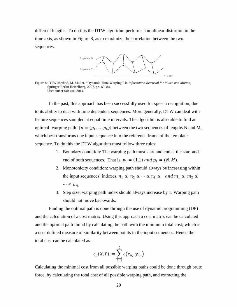
different lengths. To do this the DTW algorithm performs a nonlinear distortion in the
time axis, as shown in Figure 8, as to maximize the correlation between the two
sequences.
Figure 8: DTW Method, M. Müller, “Dynamic Time Warping,” in Information Retrieval for Music and Motion,
Springer Berlin Heidelberg, 2007, pp. 69–84.
Used under fair use, 2014.
In the past, this approach has been successfully used for speech recognition, due
to its ability to deal with time dependent sequences. More generally, DTW can deal with
feature sequences sampled at equal time intervals. The algorithm is also able to find an
optimal ‘warping path’ between the two sequences of lengths N and M,
which best transforms one input sequence into the reference frame of the template
sequence. To do this the DTW algorithm must follow three rules:
1. Boundary condition: The warping path must start and end at the start and
end of both sequences. That is, .
2. Monotonicity condition: warping path should always be increasing within
the input sequences’ indexes.
3. Step size: warping path index should always increase by 1. Warping path
should not move backwards.
Finding the optimal path is done through the use of dynamic programming (DP)
and the calculation of a cost matrix. Using this approach a cost matrix can be calculated
and the optimal path found by calculating the path with the minimum total cost; which is
a user defined measure of similarity between points in the input sequences. Hence the
total cost can be calculated as
∑ (
)
Calculating the minimal cost from all possible warping paths could be done through brute
force, by calculating the total cost of all possible warping path, and extracting the
21
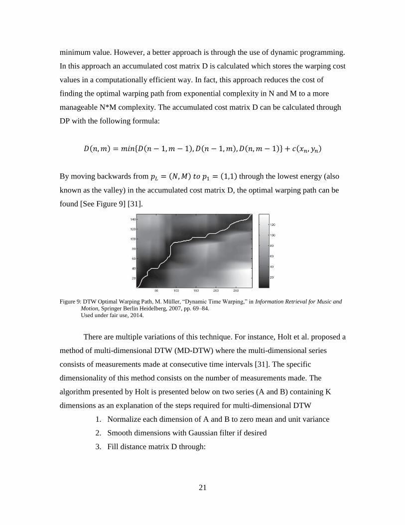
minimum value. However, a better approach is through the use of dynamic programming.
In this approach an accumulated cost matrix D is calculated which stores the warping cost
values in a computationally efficient way. In fact, this approach reduces the cost of
finding the optimal warping path from exponential complexity in N and M to a more
manageable N*M complexity. The accumulated cost matrix D can be calculated through
DP with the following formula:
{ }
By moving backwards from through the lowest energy (also
known as the valley) in the accumulated cost matrix D, the optimal warping path can be
found [See Figure 9] [31].
Figure 9: DTW Optimal Warping Path, M. Müller, “Dynamic Time Warping,” in Information Retrieval for Music and
Motion, Springer Berlin Heidelberg, 2007, pp. 69–84.
Used under fair use, 2014.
There are multiple variations of this technique. For instance, Holt et al. proposed a
method of multi-dimensional DTW (MD-DTW) where the multi-dimensional series
consists of measurements made at consecutive time intervals [31]. The specific
dimensionality of this method consists on the number of measurements made. The
algorithm presented by Holt is presented below on two series (A and B) containing K
dimensions as an explanation of the steps required for multi-dimensional DTW
1. Normalize each dimension of A and B to zero mean and unit variance
2. Smooth dimensions with Gaussian filter if desired
3. Fill distance matrix D through:
22
∑
4. Use distance matrix to find best synchronization path through standard
DTW
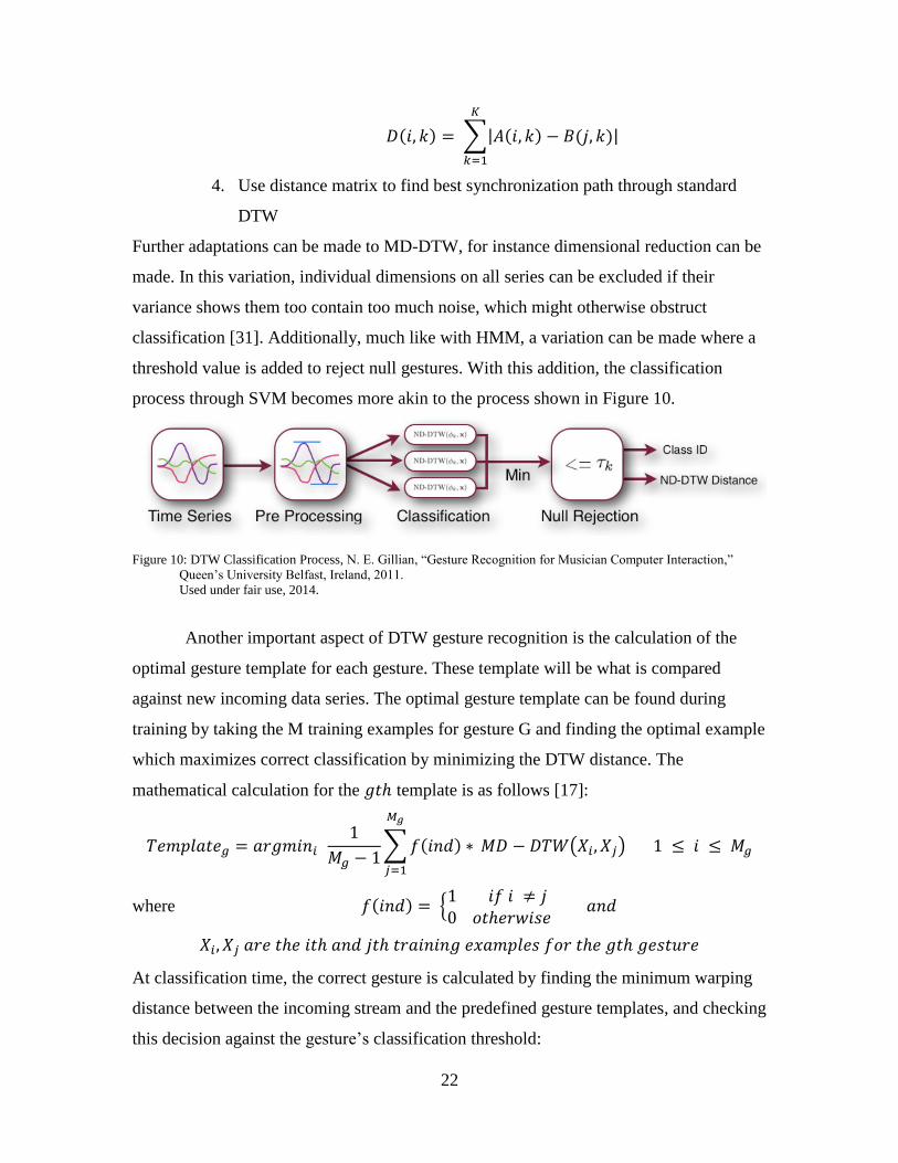
Further adaptations can be made to MD-DTW, for instance dimensional reduction can be
made. In this variation, individual dimensions on all series can be excluded if their
variance shows them too contain too much noise, which might otherwise obstruct
classification [31]. Additionally, much like with HMM, a variation can be made where a
threshold value is added to reject null gestures. With this addition, the classification
process through SVM becomes more akin to the process shown in Figure 10.
Figure 10: DTW Classification Process, N. E. Gillian, “Gesture Recognition for Musician Computer Interaction,”
Queen’s University Belfast, Ireland, 2011.
Used under fair use, 2014.
Another important aspect of DTW gesture recognition is the calculation of the
optimal gesture template for each gesture. These template will be what is compared
against new incoming data series. The optimal gesture template can be found during
training by taking the M training examples for gesture G and finding the optimal example
which maximizes correct classification by minimizing the DTW distance. The
mathematical calculation for the template is as follows [17]:
∑
( )
where {
At classification time, the correct gesture is calculated by finding the minimum warping
distance between the incoming stream and the predefined gesture templates, and checking
this decision against the gesture’s classification threshold:
23
( )
{
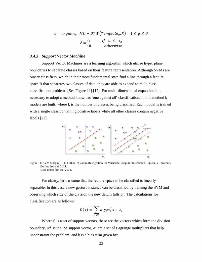
3.4.3 Support Vector Machine
Support Vector Machines are a learning algorithm which utilize hyper plane
boundaries to separate classes based on their feature representation. Although SVMs are
binary classifiers, which in their most fundamental state find a line through a feature
space R that separates two classes of data, they are able to expand to multi class
classification problems [See Figure 11] [17]. For multi-dimensional expansion it is
necessary to adopt a method known as ‘one against all’ classification. In this method k
models are built, where k is the number of classes being classified. Each model is trained
with a single class containing positive labels while all other classes contain negative
labels [22].
Figure 11: SVM Margin, N. E. Gillian, “Gesture Recognition for Musician Computer Interaction,” Queen’s University
Belfast, Ireland, 2011.
Used under fair use, 2014.
For clarity, let’s assume that the feature space to be classified is linearly
separable. In this case a new gesture instance can be classified by training the SVM and
observing which side of the division the new datum falls on. The calculations for
classification are as follows:
∑
Where S is a set of support vectors, these are the vectors which form the division
boundary, is the support vector, are a set of Lagrange multipliers that help
unconstraint the problem, and b is a bias term given by:
24
∑
Using this method a new feature vector, representing a new gesture, can be classified as:
{
Though this method was originally presented as a linear classifier, it is able to
classify non-linear/high dimensional data through the use of nonlinear kernel transforms.
Using these methods, data is mapped into a higher dimensional feature space where a
linear separation is possible. In this study two kernels will be tested. The first is the radial
basis function kernel (RBF), which has been found to offer optimal results in gesture
recognition [6]. This kernel is given by:
| |
where is a positive parameter controlling the radius of the kernel. The second is the
linear kernel given by the function:
The linear kernel is the simplest of all the kernel functions; in fact the use of the linear
kernel is often equivalent to an algorithm’s non-kernel counterpart. As seen in its
formulation above, it is given by the inner product of and plus an optional constant c
[32].
3.5 Summary
Chapter 3 has covered the three mayor parts of this thesis. First, background on
electromyography was covered, concentrating on how electrical signals are generated
from motor units during movement and how these can be captured with the use of
electrodes. Second, basic arm physiology was studied as it related to upper arm
movements and gestures; here, an emphasis was put on those muscles which could be
used for the design and control of a prosthetic arm. Finally, a large portion of this chapter
went to the study of machine learning principles as they relate to gesture recognition.
Within this section, Hidden Markov Models, Support Vector Machines, and Dynamic
Time Warping were introduced alongside their basic parts and uses.
Using the knowledge gained from this and the previous chapters, the following
chapter will setup the methods used in the current gesture recognition system design. This

25
chapter will be all inclusive, beginning with the chosen dataset, its preprocessing and
extraction of feature data, the chosen representation of this data, and the application of
each of the three learning methods to said data.

26
4 Methods
4.1 Chapter Summary
Chapter 4 will explore the methods used in conducting the experiments specific to
this thesis. First, the dataset used will be covered in depth, including how it was
collected, analyzed and segmented for use with the machine learning tools chosen. An in
depth view of the features extracted will be given, and how they relate to both to the
classifiers, and the gestures in the set. Following this, a series of experiments will be
outlined which cover the rest of the system from feature selection to the optimization of
each of the three individual classifiers.
4.2 Dataset
The decision was made to use an existing database for EMG data. The database
goes under the name of “The Ninapro Project”, it is a congregation of surface EMG and
kinematic data from 27 intact subjects over 52 movements or gestures [11]. This database
has been proposed recently as a benchmarking tool for hand prosthetics and gesture
recognition. Hence, through its use, the results of this thesis can be compared to a larger
body of work already available.
The data in the Ninapro database was collected using two separate tools. First, a
22-sensor dataglove (Cyberglove II) was used to measure kinematic data (finger
positions). This glove represents joint angles as 8-bit values, which gives an average
resolution of less than 1 degree. The Cyberglove is a standard device in virtual reality and
clinical research. Secondly, surface EMG sensors were used to collect muscular activity;
ten Deslys Trigno Wireless active double-differential electrodes (OttoBock MyoBock
13E200) were used. Using this system, EMG signals are synchronously sampled at 2
kHz; these sensors also include 3 axis accelerometers sampled at 148 Hz [12].
Ultimately, these sensors provide a signal that is amplified, bandpass-filtered, and
rectified [11]. The electrodes are evenly spaced around the forearm just below the elbow
at a fixed distance from the radiohumeral joint. Ten more sensors are placed on the flexor
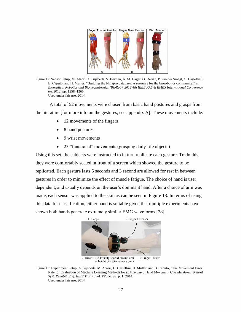
and extensor muscles [11]. The sensor locations can be seen in Figure 12, where 1
represents the equally placed electrodes, 2 are the spare electrodes, 3 corresponds to an
inclinometer and 4 is the Cyberglove II, which includes its own 22 sensors.
27
Figure 12: Sensor Setup, M. Atzori, A. Gijsberts, S. Heynen, A. M. Hager, O. Deriaz, P. van der Smagt, C. Castellini,
B. Caputo, and H. Muller, “Building the Ninapro database: A resource for the biorobotics community,” in
Biomedical Robotics and Biomechatronics (BioRob), 2012 4th IEEE RAS & EMBS International Conference
on, 2012, pp. 1258–1265.
Used under fair use, 2014.
A total of 52 movements were chosen from basic hand postures and grasps from
the literature [for more info on the gestures, see appendix A]. These movements include:
12 movements of the fingers
8 hand postures
9 wrist movements
23 “functional” movements (grasping daily-life objects)
Using this set, the subjects were instructed to in turn replicate each gesture. To do this,
they were comfortably seated in front of a screen which showed the gesture to be
replicated. Each gesture lasts 5 seconds and 3 second are allowed for rest in between
gestures in order to minimize the effect of muscle fatigue. The choice of hand is user
dependent, and usually depends on the user’s dominant hand. After a choice of arm was
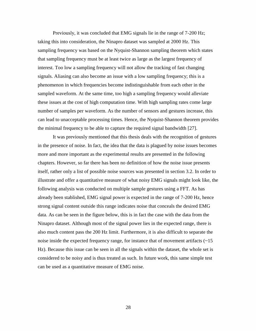
made, each sensor was applied to the skin as can be seen in Figure 13. In terms of using
this data for classification, either hand is suitable given that multiple experiments have
shown both hands generate extremely similar EMG waveforms [28].
Figure 13: Experiment Setup, A. Gijsberts, M. Atzori, C. Castellini, H. Muller, and B. Caputo, “The Movement Error
Rate for Evaluation of Machine Learning Methods for sEMG-based Hand Movement Classification,” Neural
Syst. Rehabil. Eng. IEEE Trans., vol. PP, no. 99, p. 1, 2014.
Used under fair use, 2014.
28
Previously, it was concluded that EMG signals lie in the range of 7-200 Hz;
taking this into consideration, the Ninapro dataset was sampled at 2000 Hz. This
sampling frequency was based on the Nyquist-Shannon sampling theorem which states
that sampling frequency must be at least twice as large as the largest frequency of
interest. Too low a sampling frequency will not allow the tracking of fast changing
signals. Aliasing can also become an issue with a low sampling frequency; this is a
phenomenon in which frequencies become indistinguishable from each other in the
sampled waveform. At the same time, too high a sampling frequency would alleviate
these issues at the cost of high computation time. With high sampling rates come large
number of samples per waveform. As the number of sensors and gestures increase, this
can lead to unacceptable processing times. Hence, the Nyquist-Shannon theorem provides
the minimal frequency to be able to capture the required signal bandwidth [27].
It was previously mentioned that this thesis deals with the recognition of gestures
in the presence of noise. In fact, the idea that the data is plagued by noise issues becomes
more and more important as the experimental results are presented in the following
chapters. However, so far there has been no definition of how the noise issue presents
itself, rather only a list of possible noise sources was presented in section 3.2. In order to
illustrate and offer a quantitative measure of what noisy EMG signals might look like, the
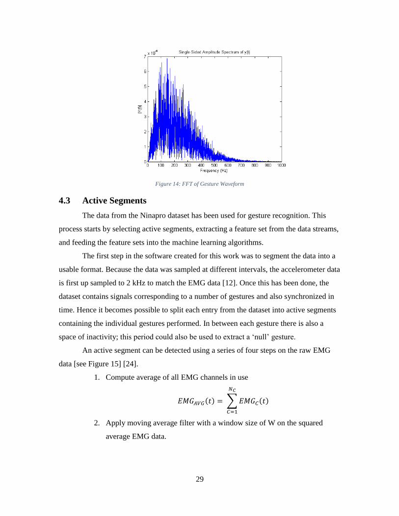
following analysis was conducted on multiple sample gestures using a FFT. As has
already been stablished, EMG signal power is expected in the range of 7-200 Hz, hence
strong signal content outside this range indicates noise that conceals the desired EMG
data. As can be seen in the figure below, this is in fact the case with the data from the
Ninapro dataset. Although most of the signal power lies in the expected range, there is
also much content pass the 200 Hz limit. Furthermore, it is also difficult to separate the
noise inside the expected frequency range, for instance that of movement artifacts (~15
Hz). Because this issue can be seen in all the signals within the dataset, the whole set is
considered to be noisy and is thus treated as such. In future work, this same simple test
can be used as a quantitative measure of EMG noise.
29
Figure 14: FFT of Gesture Waveform
4.3 Active Segments
The data from the Ninapro dataset has been used for gesture recognition. This
process starts by selecting active segments, extracting a feature set from the data streams,
and feeding the feature sets into the machine learning algorithms.
The first step in the software created for this work was to segment the data into a
usable format. Because the data was sampled at different intervals, the accelerometer data
is first up sampled to 2 kHz to match the EMG data [12]. Once this has been done, the
dataset contains signals corresponding to a number of gestures and also synchronized in
time. Hence it becomes possible to split each entry from the dataset into active segments
containing the individual gestures performed. In between each gesture there is also a
space of inactivity; this period could also be used to extract a ‘null’ gesture.
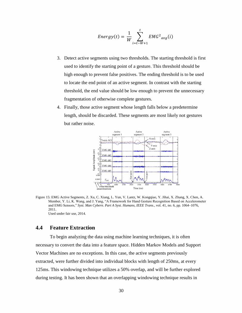
An active segment can be detected using a series of four steps on the raw EMG
data [see Figure 15] [24].
1. Compute average of all EMG channels in use
∑
2. Apply moving average filter with a window size of W on the squared
average EMG data.
30
∑
3. Detect active segments using two thresholds. The starting threshold is first
used to identify the starting point of a gesture. This threshold should be
high enough to prevent false positives. The ending threshold is to be used
to locate the end point of an active segment. In contrast with the starting
threshold, the end value should be low enough to prevent the unnecessary
fragmentation of otherwise complete gestures.
4. Finally, those active segment whose length falls below a predetermine
length, should be discarded. These segments are most likely not gestures
but rather noise.
Figure 15: EMG Active Segments, Z. Xu, C. Xiang, L. Yun, V. Lantz, W. Kongqiao, Y. Jihai, X. Zhang, X. Chen, A.
Member, Y. Li, K. Wang, and J. Yang, “A Framework for Hand Gesture Recognition Based on Accelerometer
and EMG Sensors,” Syst. Man Cybern. Part A Syst. Humans, IEEE Trans., vol. 41, no. 6, pp. 1064–1076,
2011.
Used under fair use, 2014.
4.4 Feature Extraction
To begin analyzing the data using machine learning techniques, it is often
necessary to convert the data into a feature space. Hidden Markov Models and Support
Vector Machines are no exceptions. In this case, the active segments previously
extracted, were further divided into individual blocks with length of 250ms, at every
125ms. This windowing technique utilizes a 50% overlap, and will be further explored
during testing. It has been shown that an overlapping windowing technique results in
31
better performance than a disjointed one [33]. Furthermore, each channel within these
windows is filtered by a Hamming window in order to remove unwanted effects from
edge discontinuities [24]. The size of the window to test is often debated in EMG
literature. The important aspects to remember are that the window size must be long
enough to capture the temporal pattern in the signal, while at the same time being short
enough to maintain the assumption of signal stationarity [34].
Some of the most popular and widely acknowledge features are listed below. They
have been chosen for their ability to differentiate EMG signal based gestures. For
instance, the standard deviation feature has been shown to be a good measure muscle
activity, as it is well correlated to signal energy while remaining invariant to amplitude
differences. Other commonly used features are number of zero crossings, slope sign
change, and waveform length [10]. For a more detailed view into popular EMG features
and their mathematical representation, please see appendix B [35].
1. Integrated EMG (IEMG): Calculated as the summation of the signal’s absolute
value. Often used as an active segment detector [36]
∑
Where x is an EMG signal and N is the length of that signal
2. Mean Absolute Value (MAV): Estimate of the mean absolute value of signal.
Frequently used to mark onset of a gesture [37]
∑
3. Single Square Integral (SSI): Representation of the energy in the EMG signal [36]
∑
4. Variance of EMG (VAR): Estimate of the power content of signal. [7]
32
∑
Where is the signal mean.
5. Root Mean Square (RMS): Estimate of standard deviation of signal. Also
estimates power content of signal. [7]
√
∑
6. Waveform Length (WL): Cumulative length of signal. Contains information about
signal frequency, amplitude, and duration. [7]
∑
7. Willison Amplitude (WAMP): Measures motor unit activity while ignoring noise
as defined by the threshold level. [7]
∑ , {
8. Log Detector (LOG): Provides an estimate of the force exerted by a muscle [35]
[20]
∑
9. Slope Sign Change (SSC): Estimates frequency content of signal. Ignores noise
as defined by threshold value. [7]
∑
Where
{
10. Zero Crossing (ZC): Estimates frequency content of signal. Ignores noise as
defined by threshold value. [7]
∑
33
Where
{
Extracting these features from the dataset was done with custom code based on
the “Myoelectric Control Development Toolbox” put together by Chan et al. This toolbox
is designed to allow researchers to have a common ground for comparison of EMG
classifiers. The toolbox also contains other miscellaneous routines to facilitate filtering of
raw EMG signals, as well as some tools for dimensionality reduction [38].
Three of the features extracted from the data require the previous calculation of a
threshold value. This empirically found value is meant to facilitate the extraction of
signal information whilst ignoring the effects of noise. In order to calculate the optimal
value for this threshold, two tests were performed. The first is a process very similar to
the feature selection wrapper method that will be explored in the feature selection section,
while the second is a method based on the commonly used signal to noise ratio in signal
processing.
For the first pass as the at threshold selection, the classification accuracy based on
an SVM wrapper was used to test different threshold values. Using this method and
averaging over many folds in k-fold cross validation, a consisted pattern could be
extracted. However, the time complexity of this method quickly became apparent and
diminished the ability to test a wide array of thresholds. To overcome the time constraints
of the previous method, the second approach was utilized based on the signal to noise
difference for each feature [7]. This method works by calculating a feature’s average
value during activity(S) and rest (N). Then, for a range of threshold values, the difference
of signal(S) to noise (N) is calculated, with the highest S-N value giving the optimal
threshold.
4.5 Feature Selection
In order to optimize classification accuracy, the extracted features were further
reduced in number using feature selection methods. Ideally, every subset combination of
features would be investigated and the optimum combination chosen. However, even
with the thirteen features this work deals with, an exhaustive search such as this would
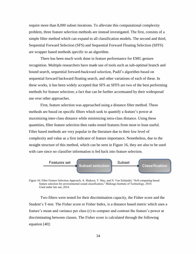
34
require more than 8,000 subset iterations. To alleviate this computational complexity
problem, three feature selection methods are instead investigated. The first, consists of a
simple filter method which can expand to all classification models. The second and third,
Sequential Forward Selection (SFS) and Sequential Forward Floating Selection (SFFS)
are wrapper based methods specific to an algorithm.
There has been much work done in feature performance for EMG gesture
recognition. Multiple researchers have made use of tools such as sub-optimal branch and
bound search, sequential forward-backward selection, Pudil’s algorithm based on
sequential forward backward floating search, and other variations of each of these. In
these works, it has been widely accepted that SFS an SFFS are two of the best performing
methods for feature selection; a fact that can be further accentuated by their widespread
use over other approaches.
First, feature selection was approached using a distance filter method. These
methods are based on specific filters which seek to quantify a feature’s power at
maximizing inter-class distance while minimizing intra-class distance. Using these
quantities, filter feature selection then ranks tested features from most to least useful.
Filter based methods are very popular in the literature due to their low level of
complexity and value as a first indicator of feature importance. Nonetheless, due to the
straight structure of this method, which can be seen in Figure 16, they are also to be used
with care since no classifier information is fed back into feature selection.
Figure 16: Filter Feature Selection Approach, A. Shakoor, T. May, and N. Van Schijndel, “Soft computing based
feature selection for environmental sound classification,” Blekinge Institute of Technology, 2010.
Used under fair use, 2014.
Two filters were tested for their discrimination capacity, the Fisher score and the
Student’s T-test. The Fisher score or Fisher Index, is a distance based metric which uses a
feature’s mean and variance per class (c) to compare and contrast the feature’s power at
discriminating between classes. The Fisher score is calculated through the following
equation [40]:
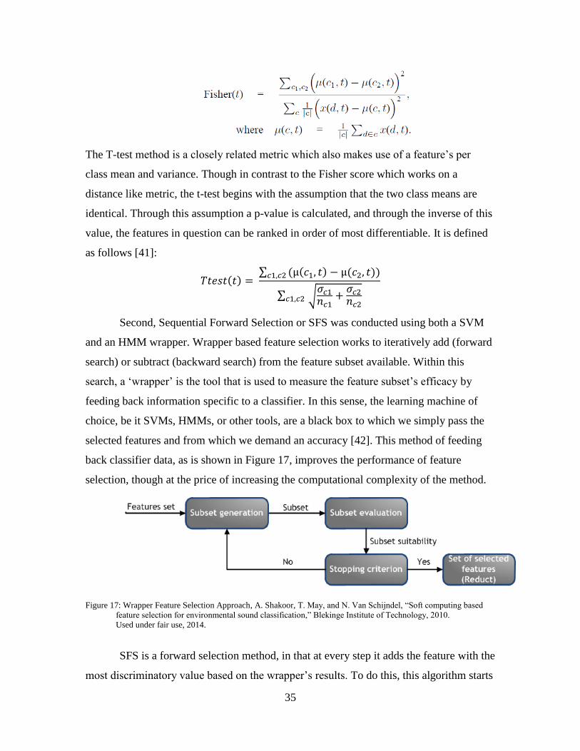
35
The T-test method is a closely related metric which also makes use of a feature’s per
class mean and variance. Though in contrast to the Fisher score which works on a
distance like metric, the t-test begins with the assumption that the two class means are
identical. Through this assumption a p-value is calculated, and through the inverse of this
value, the features in question can be ranked in order of most differentiable. It is defined
as follows [41]:
∑
∑ √
Second, Sequential Forward Selection or SFS was conducted using both a SVM
and an HMM wrapper. Wrapper based feature selection works to iteratively add (forward
search) or subtract (backward search) from the feature subset available. Within this
search, a ‘wrapper’ is the tool that is used to measure the feature subset’s efficacy by
feeding back information specific to a classifier. In this sense, the learning machine of
choice, be it SVMs, HMMs, or other tools, are a black box to which we simply pass the
selected features and from which we demand an accuracy [42]. This method of feeding
back classifier data, as is shown in Figure 17, improves the performance of feature
selection, though at the price of increasing the computational complexity of the method.
Figure 17: Wrapper Feature Selection Approach, A. Shakoor, T. May, and N. Van Schijndel, “Soft computing based
feature selection for environmental sound classification,” Blekinge Institute of Technology, 2010.
Used under fair use, 2014.
SFS is a forward selection method, in that at every step it adds the feature with the
most discriminatory value based on the wrapper’s results. To do this, this algorithm starts
36
with a null subset of features and at every iteration adds and tests every feature not yet in
the final subset through the chosen wrapper and records the average accuracy. It then
picks and adds to the final subset, the feature with the best improvement. By doing this at
every iteration the SFS algorithm ranks the best features and records their classification
power. It then becomes up to the user to either place a limit on how many features to add
to the final subset or at which classification accuracy to break the cycle [19].
Finally, the SFFS wrapper method was also used to automatically extract the
optimum feature subset size. In this case a black box wrapper is also used; though the
choice of stopping criterion is simplified for the user. This method works by combining
the SFS method with a backwards step meant to simplify the model at every iteration.
First, at the beginning of every iteration the method works just like the SFS method. Each
feature not yet in the final subset is added and tested using the selected wrapper. The
feature which offers the maximum improvement is then added to the subset list. At this
point, instead of moving on to the next iteration step, like the SFS method, the SFFS
method also incorporates a backwards step in which every feature is systematically
removed from the subset. If the subset is found to improve by the removal of a feature,
then that feature is permanently removed. By following these two steps at every iteration,
the SFFS method improves on the performance of the SFS method in that the smallest
and most powerful feature subset is chosen without the user having to indicate a number
of features for the final subset [19].
4.6 Hidden Markov Models
Working with HMMs requires fine-tuning certain parameters to optimize
classification. In the case of gesture recognition there are four main parameters this work
investigated:
1. Number of states per model
2. Number of output symbols per model
3. Number of states that the model is allowed to skip over
4. Optimal feature representation
Additionally, two more tests were conducted to further compare the results and optimize
the procedure.
37
5. Discriminatory power for different numbers of classes
6. Minimum number of training observations
4.6.1 Vector Discretization
Because of the choice to use discrete Hidden Markov Models, as opposed to their
continuous counterparts, it is necessary to discretize all observation sequences before
completing any of the desired tests. In order to do this, the feature vectors which result
from feature extraction must be clustered and separated into a number of discrete clusters.
The k-means clustering method is used in this approach in order to divide the set of n
training observation into the desired number of clusters [43]. Next, testing observations
must also be split into these clusters at test time. In order to do this, there are two main
methods available in the literature: the k-nearest neighbor approach and the closest
cluster center approach [17] [44].
K-nearest neighbor (KNN) is a method through which a new observation is placed
in the training feature space and its k-nearest neighbors are studied. These neighbors are
checked for their cluster membership, and the most common membership is applied to
the new datum [45]. In contrast, the closest cluster method makes use of the previously
calculated training cluster centers. A new datum is awarded a cluster membership by
placing it in the training feature space and finding the closest (usually in Euclidian
distance) cluster center to it.
Still, other researchers argue towards refraining from the use of extracted features
and k-means for clustering; arguing that EMG data is already soundly setup for
discretization based on the SAX vector quantization approach [17]. SAX or Symbolic
Aggregate Approximation is a method that alleviates noise issues inherent to k-means.
Furthermore, if desirable SAX quantized data can be further quantized using k-means.
SAX is a process through which a single dimensional time series
, of length L is able to be discretized to a secondary series ,
of length S, where S < L. The new series contains discrete values within a predefined and
finite range [See Figure 18] [17]. In the case where the desired raw input is multi-
dimensional, the SAX algorithm is applied to every dimension separately. Below are the
steps taken for proper SAX discretization:
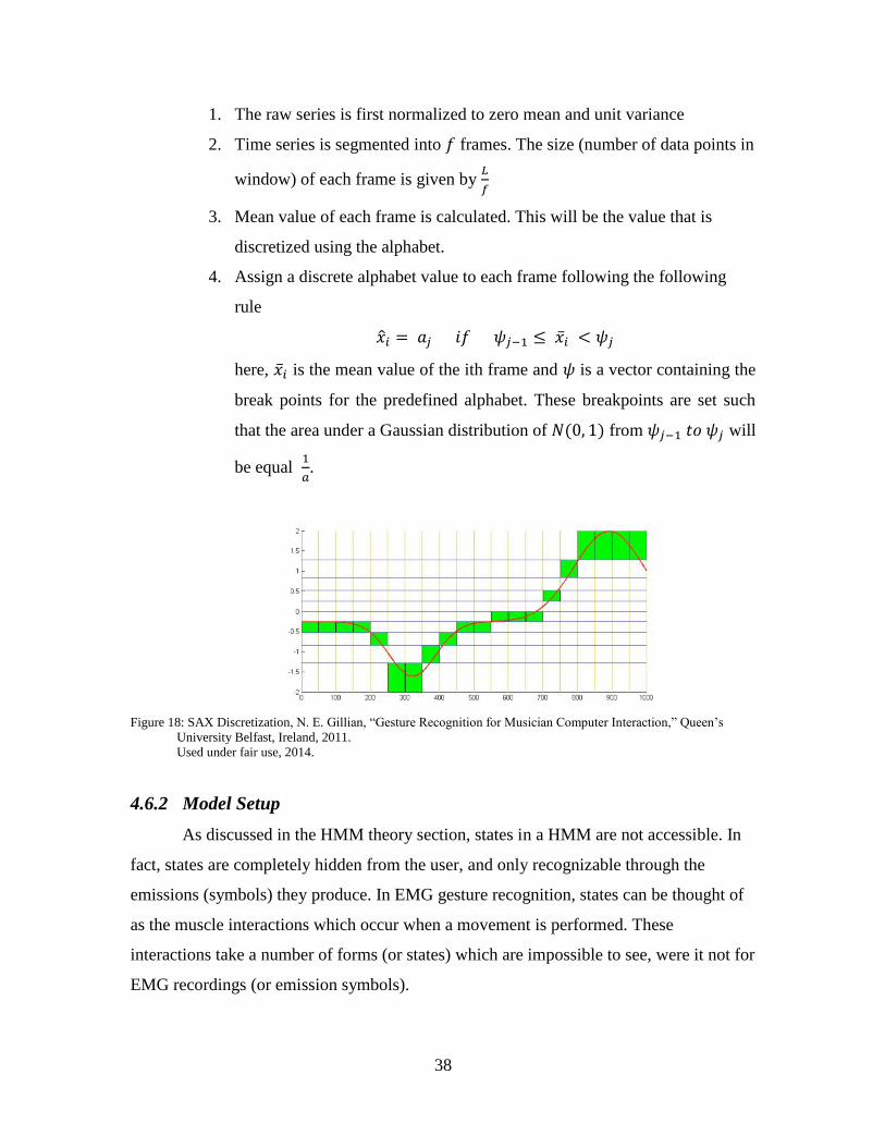
38
1. The raw series is first normalized to zero mean and unit variance
2. Time series is segmented into frames. The size (number of data points in
window) of each frame is given by
3. Mean value of each frame is calculated. This will be the value that is
discretized using the alphabet.
4. Assign a discrete alphabet value to each frame following the following
rule
here, is the mean value of the ith frame and is a vector containing the
break points for the predefined alphabet. These breakpoints are set such
that the area under a Gaussian distribution of from will
be equal
.
Figure 18: SAX Discretization, N. E. Gillian, “Gesture Recognition for Musician Computer Interaction,” Queen’s
University Belfast, Ireland, 2011.
Used under fair use, 2014.
4.6.2 Model Setup
As discussed in the HMM theory section, states in a HMM are not accessible. In
fact, states are completely hidden from the user, and only recognizable through the
emissions (symbols) they produce. In EMG gesture recognition, states can be thought of
as the muscle interactions which occur when a movement is performed. These
interactions take a number of forms (or states) which are impossible to see, were it not for
EMG recordings (or emission symbols).
39
Training an HMM thus requires an estimation of the number of hidden states
present in the real world phenomenon, as well as the number of emissions each state is
viable to produce. In order to gauge the number of states and the number of emissions
necessary for gesture recognition, (where ) models were trained
using a k-fold training method. Each model followed a left-to-right approach, allowing
for a single state to be skipped; each model was also constructed using a nearest cluster
discretization method. For each model an average accuracy was calculated for all folds.
By using a grid search over the number of state and symbols, with states and symbol
ranging from 9 to 27, it was possible to estimate the optimal values for the final
optimized models.
4.6.3 Left to Right vs. Ergodic Models
Even though previous works in gesture and speech recognition have concluded
that a left to right model structure is preferable over an ergodic structure, there have also
been works which speak to the flexibility of each structure [17]. As seen previously, a
left to right structure limits the model from skipping over states during the training phase.
However, strictly enforcing that states have to be sequential might make the model too
rigid for proper generalization.
In order to test this, a series of models were created using a k-fold training method
(where ). Each model iteration allowed an integer number of skipped states,
ranging from 3 to 15. At each iteration, the models’ accuracy were averaged over all
folds.
4.6.4 Effect of Increasing Vocabulary
Depending on the application for which gesture recognition is being applied, a
different number of gestures or classes, are to be needed. For instance, if the task is to
design a simple sign language translator, then a gesture recognition system needs around
26 recognizable classes. If the task is to recognize military hand signals, then a smaller
number would be required.
The number of classes is important to keep in mind considering that detrimental
effect that a large number of classes can have on recognition and classification. A large
number of classes makes the classification problem more difficult and reduces accuracy
40
rates. Thus, when designing a new system, it becomes important to study the maximum
number of classes that the system is capable of handling under acceptable classification
results. To test for this number, a separate test was conducted which calculated the
average cross validation ratio using 10 fold cross validation while varying the number of
classes being tested.
4.6.5 Minimum Required Training Data
Another important parameter of a gesture recognition system is the number of
training instances that are required for optimal results. This parameter, unlike other
parameters being studied, has an effect not only on the eventual results of the system, but
also on the ease of setup. Even if the system resulted in near perfect classification
accuracy, long setup times could prove harmful to the user experience and even deter
possible users from the system. On the other hand, if the system requires little training
data, then it becomes much more transparent and inviting to wide use by the public.
In the case of the current system, a number of tests were completed to identify the
necessary number of training examples. From these tests, an optimal number of training
iterations was identified which maximized accuracy while at the same time minimizing
computation time.
4.6.6 Optimized Model
Finally, a final test was conducted with the previously identified parameters
which optimize gesture identification. Two variations of this test were performed to test
out a final optimization technique. This last parameter has been the source of debate in
the gesture recognition community. It is the difference between using a null gesture
model as is often done in speech recognition with silence models [17] or using a
validation threshold for rejecting null sequences.
While the two approaches differ drastically in their setup and implementation,
they work toward the same end. In both cases, the goal is to recognize when a gesture is
not being performed. For instance, if a subject is simply swinging an arm during a
walking motion, this “gesture” should not be classified as some intentional movement.
Some works have tried to resolve the issue of the null gesture by incorporating a trigger
key into their systems [17]. Using this approach, an end user of the system, would have
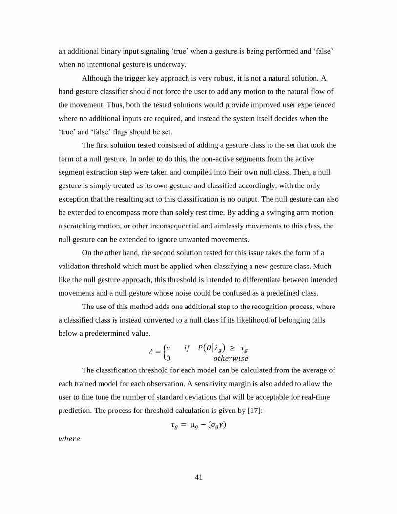
41
an additional binary input signaling ‘true’ when a gesture is being performed and ‘false’
when no intentional gesture is underway.
Although the trigger key approach is very robust, it is not a natural solution. A
hand gesture classifier should not force the user to add any motion to the natural flow of
the movement. Thus, both the tested solutions would provide improved user experienced
where no additional inputs are required, and instead the system itself decides when the
‘true’ and ‘false’ flags should be set.
The first solution tested consisted of adding a gesture class to the set that took the
form of a null gesture. In order to do this, the non-active segments from the active
segment extraction step were taken and compiled into their own null class. Then, a null
gesture is simply treated as its own gesture and classified accordingly, with the only
exception that the resulting act to this classification is no output. The null gesture can also
be extended to encompass more than solely rest time. By adding a swinging arm motion,
a scratching motion, or other inconsequential and aimlessly movements to this class, the
null gesture can be extended to ignore unwanted movements.
On the other hand, the second solution tested for this issue takes the form of a
validation threshold which must be applied when classifying a new gesture class. Much
like the null gesture approach, this threshold is intended to differentiate between intended
movements and a null gesture whose noise could be confused as a predefined class.
The use of this method adds one additional step to the recognition process, where
a classified class is instead converted to a null class if its likelihood of belonging falls
below a predetermined value.
{ ( | )
The classification threshold for each model can be calculated from the average of
each trained model for each observation. A sensitivity margin is also added to allow the
user to fine tune the number of standard deviations that will be acceptable for real-time
prediction. The process for threshold calculation is given by [17]:
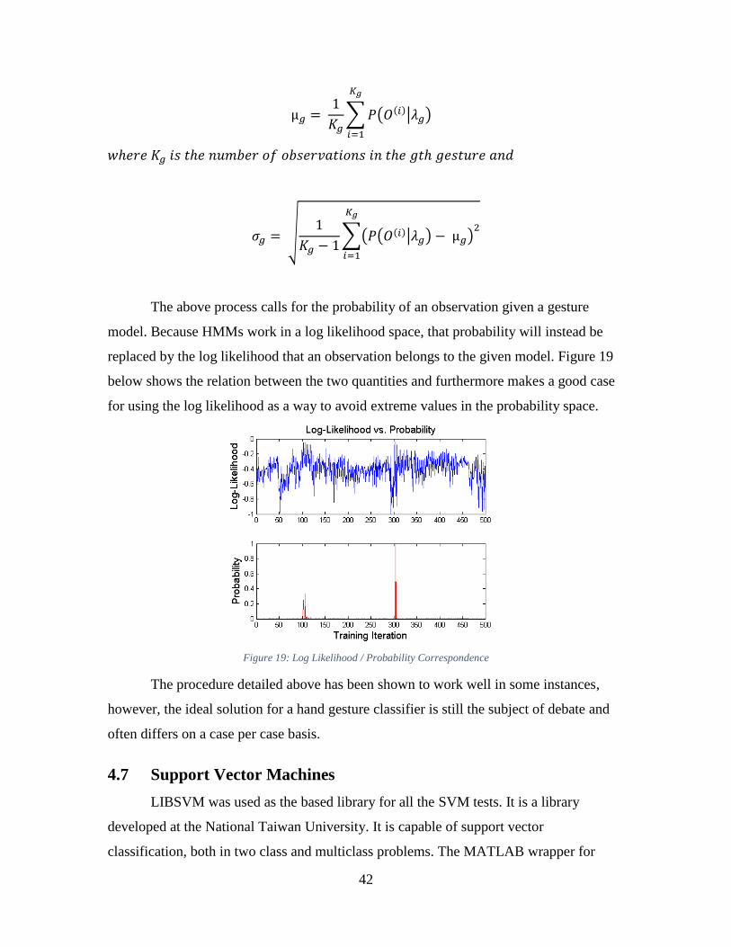
42
∑ ( | )
√
∑( ( | ) )
The above process calls for the probability of an observation given a gesture
model. Because HMMs work in a log likelihood space, that probability will instead be
replaced by the log likelihood that an observation belongs to the given model. Figure 19
below shows the relation between the two quantities and furthermore makes a good case
for using the log likelihood as a way to avoid extreme values in the probability space.
Figure 19: Log Likelihood / Probability Correspondence
The procedure detailed above has been shown to work well in some instances,
however, the ideal solution for a hand gesture classifier is still the subject of debate and
often differs on a case per case basis.
4.7 Support Vector Machines
LIBSVM was used as the based library for all the SVM tests. It is a library
developed at the National Taiwan University. It is capable of support vector
classification, both in two class and multiclass problems. The MATLAB wrapper for
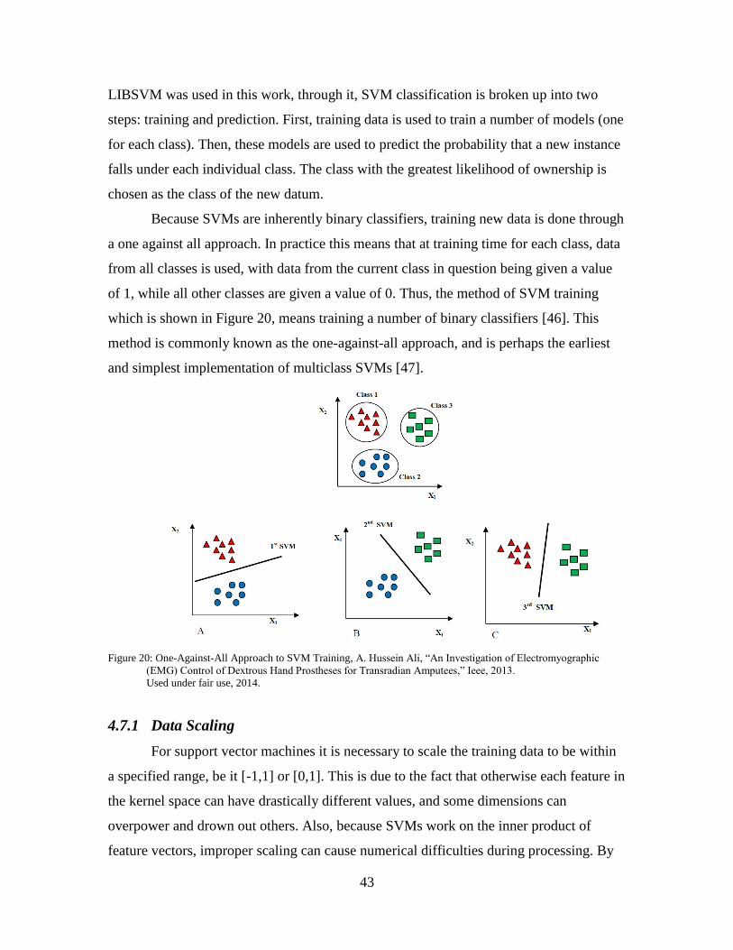
43
LIBSVM was used in this work, through it, SVM classification is broken up into two
steps: training and prediction. First, training data is used to train a number of models (one
for each class). Then, these models are used to predict the probability that a new instance
falls under each individual class. The class with the greatest likelihood of ownership is
chosen as the class of the new datum.
Because SVMs are inherently binary classifiers, training new data is done through
a one against all approach. In practice this means that at training time for each class, data
from all classes is used, with data from the current class in question being given a value
of 1, while all other classes are given a value of 0. Thus, the method of SVM training
which is shown in Figure 20, means training a number of binary classifiers [46]. This
method is commonly known as the one-against-all approach, and is perhaps the earliest
and simplest implementation of multiclass SVMs [47].
Figure 20: One-Against-All Approach to SVM Training, A. Hussein Ali, “An Investigation of Electromyographic
(EMG) Control of Dextrous Hand Prostheses for Transradian Amputees,” Ieee, 2013.
Used under fair use, 2014.
4.7.1 Data Scaling
For support vector machines it is necessary to scale the training data to be within
a specified range, be it [-1,1] or [0,1]. This is due to the fact that otherwise each feature in
the kernel space can have drastically different values, and some dimensions can
overpower and drown out others. Also, because SVMs work on the inner product of
feature vectors, improper scaling can cause numerical difficulties during processing. By
44
scaling each dimension to the same range, these problems can be avoided while ensuring
that all dimensions are weighted equally.
Care must also be taken to properly scale the data during model generation. That
is to say that testing and training data must be scaled in the same manner. This can also
be viewed from the fact that no prior knowledge can be assumed form the testing data.
Thus, the same scaling factors used in the training data must also be used for testing data.
For instance, assume that a training feature with a range of [-100, +100] is to be scaled to
[-1, +1], then if the same feature during testing lies in the range of [-150,+50], it must be
scaled to [-1.5,+0.5] [48].
4.7.2 Kernel Test
In order to optimize the required SVM parameters, a grid search was conducted
using a 10 fold cross validation approach for each grid point. Both the linear and RBF
kernels were tested for classification accuracy, with the linear variant serving as a
comparison step for the more robust and popular RBF kernel. The C and gamma
parameters were varied during in each step as powers of two (for a remainder of what
these terms are, please refer back to chapter 3)[34]. From this search both the most
powerful kernel and its most robust parameters were then extracted for use in the final
SVM classifier.
4.7.3 Effect of Increasing Vocabulary
As was already reviewed with HMM classifiers, there is a need to study the power
of a classifier to a number of different classes. This means studying how the performance
of classification decreases with an increasing number of classes to distinguish. In order to
quantify these changes, a test was conducted which varied the number of classes to
identify from 4 to 18. This test was conducted using the best performing kernel from the
previous experiment, 10 fold cross validation, and a large enough number of training
samples for proper training.
4.7.4 Minimum Required Training Data
The last test necessary before a final method can be put together, is the calculation
of the required amount of training data for proper training. The corresponding test was
45
conducted using a 10 fold cross validation approach for training, as well as being tested
with both the linear and RBF kernels. At each run, a constant number of testing samples
was extracted from the available data in order to minimize any bias which might be
introduced by varying the number of testing samples.
4.7.5 Optimized Model
Once the previous results were consolidated, a final test was conducted for overall
classification accuracy. These test results served as the basis for calculating the average
classification ratio, as well as the overall precision and recall. This test was also used as a
time trial for comparison against the HMM classifier. One aspect that was not included in
this test, was the comparison between the EMG defined null gesture vs. the threshold
nullifying method. This is because, unlike with the HMM classifier, there isn’t a good
metric for determining a class instance’s distance from the model. Instead, the EMG
defined null gesture was used as part of the given class set.
4.8 Dynamic Time Warping
The first step in the process of utilizing the DTW approach consists of the
preparation of the data into a form feasible for the computational complexity that results
from a method involving constant grid searches. Alongside data representation, a useful
number of training examples or iterations must also be finalized. Too many class example
sequences would result in training times that are too long for proper use; on the other
hand, too few class examples might not capture the cleanest version of each class.
Arriving at a proper number of training examples requires some empirical data. It is also
a value very dependent on the amount of computation power and time available. For this
work, 15 iterations were chosen. Any more than this, and the method required too much
processing time for it to be useful.
As has already been seen, implementing DTW in a multiclass classification
setting involves the repeated use of the DTW method over a number of sequences. First,
a number of iteration examples is collected for each gesture class and preprocessed.
Second, these example sequences must be compared against each other in order to
calculate the template gesture. As reviewed in section 3.4.2, the class template is found
by finding the sequence that minimizes the iteration distance for every gesture. This is
46
done by comparing each example sequence for a gesture against every other sequence for
that class and collecting the resulting DTW distances. The iteration that results in the
minimum overall distance is then chosen to represent the class. Another description of
this method might be to think of the template that is chosen as the most general of the
example set. Because it shares the most with its fellow class members, the template can
be considered the iteration with the least amount of noise, and the one which represents
the motion in the way in which it was intended. As a side note of this part of the process,
while a template is being calculated, the values for the overall distance can also be
recorded alongside each individual distance between the template and its fellow class
members. These distances are then used for to find the mean and the standard deviation
of the distance data. The use of these two statistics will be seen shortly.
4.8.1 Data Preparation
Two methods were tested for data preprocessing. The first consists of both down
sampling and low pass filtering the raw data Through this method the sampling rate of a
sequence of data is effectively truncated without adding any aliasing issues to the data
[17]. The second method makes the use of the SAX algorithm, the details of which were
covered in section 4.6.1. As a reminder, the SAX method consists of a way to down
sample data through the grouping of similar terms in both time and amplitude. In both
these approaches the amount of down sampling can be fine-tuned either by choosing a
down sampling factor, or by hardcoding a set number of frames and amplitude range for a
sequence.
4.8.2 Threshold calculation
As with HMM, the classification threshold can be computed at the time of
training with the use of training examples. The threshold value is intended to remove any
classifications which fall below the training standard. In order to do this, a threshold is
calculated at post processing time with the mean and standard deviation data collected
during training time. The threshold is calculated as follows:
Where is a user defined number of standard deviations suitable for classification. The
mean and standard deviations for each training example are calculated through the
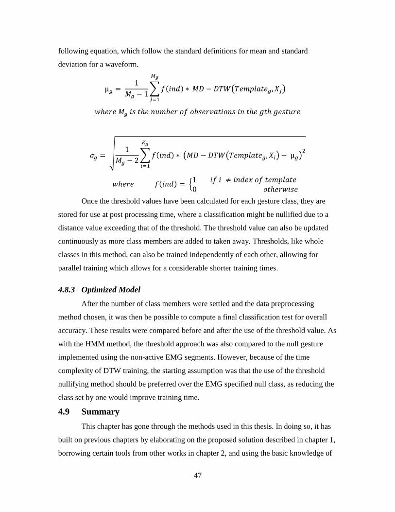
47
following equation, which follow the standard definitions for mean and standard
deviation for a waveform.
∑
( )
√
∑ ( ( ) )
{
Once the threshold values have been calculated for each gesture class, they are
stored for use at post processing time, where a classification might be nullified due to a
distance value exceeding that of the threshold. The threshold value can also be updated
continuously as more class members are added to taken away. Thresholds, like whole
classes in this method, can also be trained independently of each other, allowing for
parallel training which allows for a considerable shorter training times.
4.8.3 Optimized Model
After the number of class members were settled and the data preprocessing
method chosen, it was then be possible to compute a final classification test for overall
accuracy. These results were compared before and after the use of the threshold value. As
with the HMM method, the threshold approach was also compared to the null gesture
implemented using the non-active EMG segments. However, because of the time
complexity of DTW training, the starting assumption was that the use of the threshold
nullifying method should be preferred over the EMG specified null class, as reducing the
class set by one would improve training time.
4.9 Summary
This chapter has gone through the methods used in this thesis. In doing so, it has
built on previous chapters by elaborating on the proposed solution described in chapter 1,
borrowing certain tools from other works in chapter 2, and using the basic knowledge of

48
chapter 3. More importantly this chapter has also covered important implementation
details, such as feature formulations, and libraries uses for machine learning. This chapter
is one of the most important, given that it covers all the aspects that this author thought
important when designing a new gesture recognition system. The experiments which
have been laid out in this chapter will now be further studied in the following chapter
alongside their results and the optimized models which spring forth for each of the three
learning methods.

49
5 Results
5.1 Chapter Summary
Chapter 5 of this work presents the results achieved through the experiments
described in the previous chapter. It begins with studies done on feature selection and
representation, and goes on to test results for each of the three classifiers: DTW, HMMs,
and SVMs.
In order to contrast the three learning approaches it is necessary to stablish a
standard set of parameters that can be calculated across experiments and are
representative of the overall results of each. As such, three classification errors were used
from the work by Gillian, to evaluate the classification and recognition rates for each
algorithm [17]:
Average Cross Validation Ratio: classifier performance across all
participants
∑
Average Precision Ratio: Performance of exactness of classifier for each
gesture over all participants
Average Recall Ratio: Performance of classifier over specific gesture for
all participants
In all of these formulas, K is the number of cross validation folds.
Another tool which will be used to evaluate each classifier’s performance, is the
popularly used confusion matrix. This tool is often used to visually assess a classifier’s
performance since it quickly demonstrates correct and incorrect classifications on a per
class basis. Below is an example of a confusion matrix, the basic idea is to count the
number of outcome classifications per class on the ‘Output’ axis (x-axis) against the
correct classification on the ‘Input’ axis (y-axis). By doing this, a perfect classifier would
have 100% classification count on the main diagonal, and 0% everywhere else. Instead,
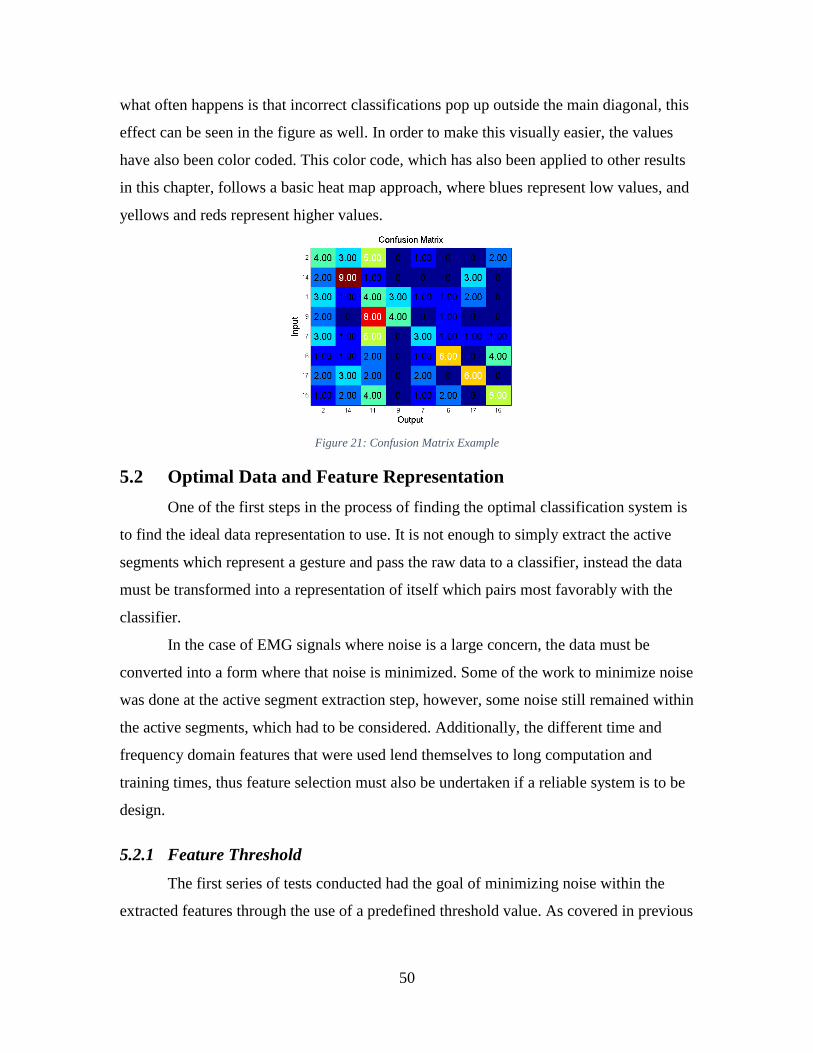
50
what often happens is that incorrect classifications pop up outside the main diagonal, this
effect can be seen in the figure as well. In order to make this visually easier, the values
have also been color coded. This color code, which has also been applied to other results
in this chapter, follows a basic heat map approach, where blues represent low values, and
yellows and reds represent higher values.
Figure 21: Confusion Matrix Example
5.2 Optimal Data and Feature Representation
One of the first steps in the process of finding the optimal classification system is
to find the ideal data representation to use. It is not enough to simply extract the active
segments which represent a gesture and pass the raw data to a classifier, instead the data
must be transformed into a representation of itself which pairs most favorably with the
classifier.
In the case of EMG signals where noise is a large concern, the data must be
converted into a form where that noise is minimized. Some of the work to minimize noise
was done at the active segment extraction step, however, some noise still remained within
the active segments, which had to be considered. Additionally, the different time and
frequency domain features that were used lend themselves to long computation and
training times, thus feature selection must also be undertaken if a reliable system is to be
design.
5.2.1 Feature Threshold
The first series of tests conducted had the goal of minimizing noise within the
extracted features through the use of a predefined threshold value. As covered in previous
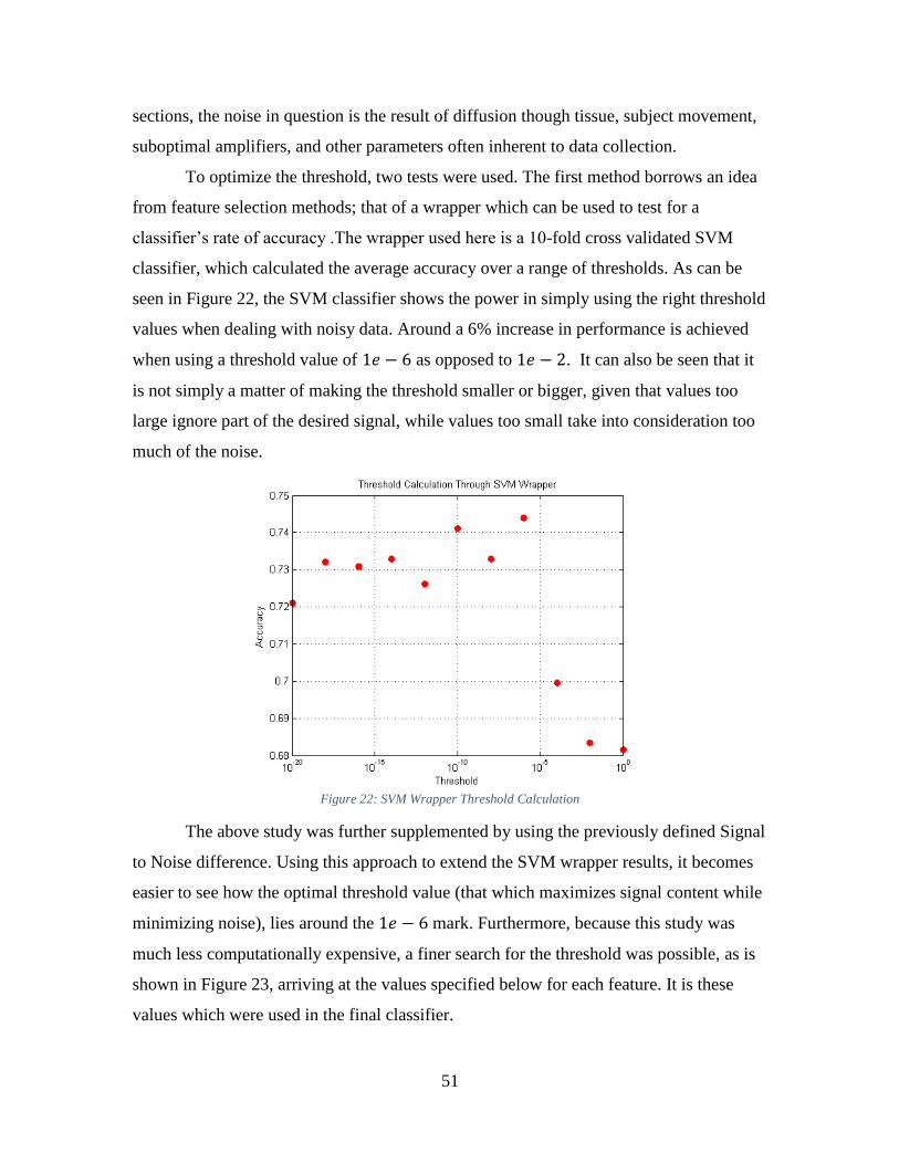
51
sections, the noise in question is the result of diffusion though tissue, subject movement,
suboptimal amplifiers, and other parameters often inherent to data collection.
To optimize the threshold, two tests were used. The first method borrows an idea
from feature selection methods; that of a wrapper which can be used to test for a
classifier’s rate of accuracy .The wrapper used here is a 10-fold cross validated SVM
classifier, which calculated the average accuracy over a range of thresholds. As can be
seen in Figure 22, the SVM classifier shows the power in simply using the right threshold
values when dealing with noisy data. Around a 6% increase in performance is achieved
when using a threshold value of as opposed to . It can also be seen that it
is not simply a matter of making the threshold smaller or bigger, given that values too
large ignore part of the desired signal, while values too small take into consideration too
much of the noise.
Figure 22: SVM Wrapper Threshold Calculation
The above study was further supplemented by using the previously defined Signal
to Noise difference. Using this approach to extend the SVM wrapper results, it becomes
easier to see how the optimal threshold value (that which maximizes signal content while
minimizing noise), lies around the mark. Furthermore, because this study was
much less computationally expensive, a finer search for the threshold was possible, as is
shown in Figure 23, arriving at the values specified below for each feature. It is these
values which were used in the final classifier.
52
Figure 23: Signal to Noise Difference Threshold Calculation
5.2.2 Number of frames
Another part of data representation which must be tested, lies in the number of
frames an active segment must be split into. Splitting a gesture iteration into multiple
segments is necessary for two reasons. First, most of the features being used deal with
overall signal amplitudes. Even though this is exactly what we want, it also means that
extracting features on whole signals can be misleading, as mirrored signals will have the
exact same feature representation. Second, when it comes to gesture recognition, much
like in speech recognition, much of the information that is sought comes from the
temporal variations present in the signal. Because of these two reasons, it is detrimental
to use a whole signal for feature extraction, instead the signal is broken up into a
specified number of frames. In the case of HMMs, the signal is often split into frames of
a certain time duration, however this leads to inconsistent feature vector lengths. On the
other hand, in the case of SVMs which require equal size feature vectors, signals are split
up into a set number of frames.
Once again using an SVM wrapper for average classification, a test was
performed to study the effect of the number of frames in the overall system’s
performance. Figure 24 below show how once again, a simple change can have a
consequential effect on performance. Simply varying the number of frames resulted in a
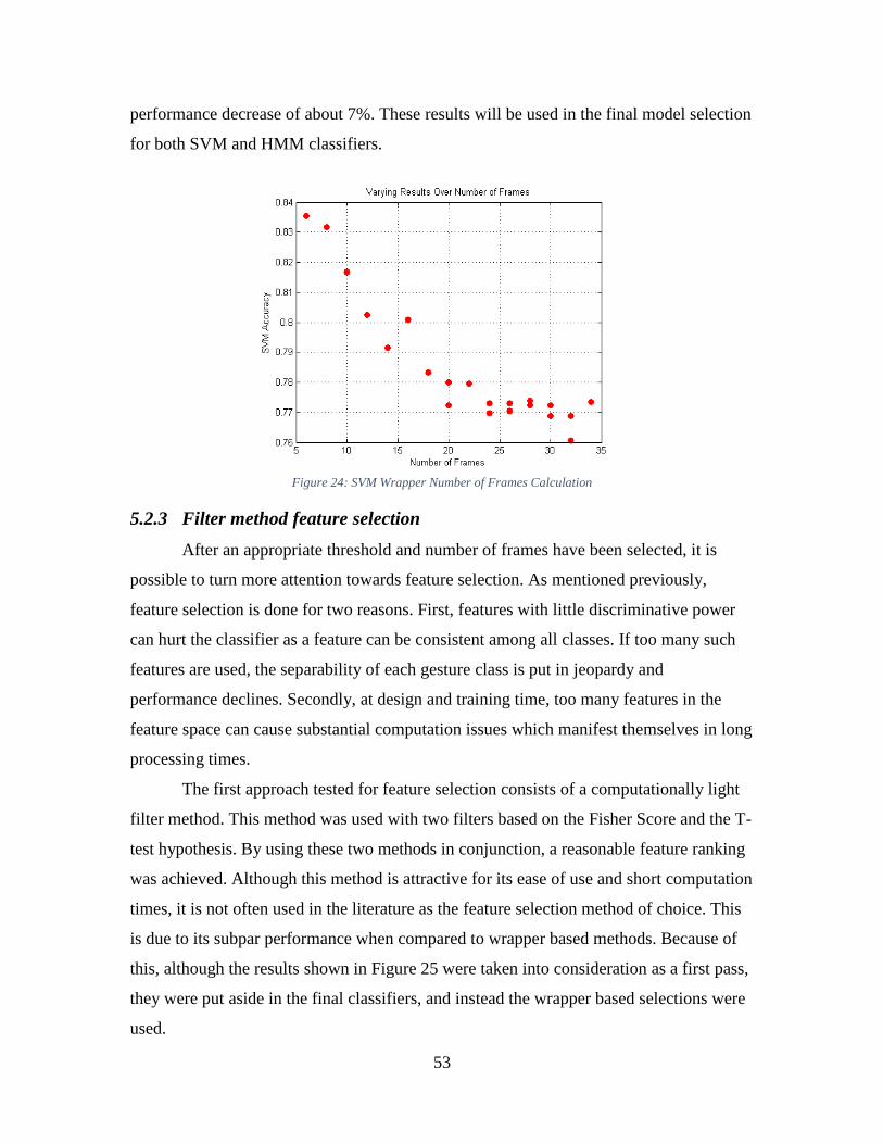
53
performance decrease of about 7%. These results will be used in the final model selection
for both SVM and HMM classifiers.
Figure 24: SVM Wrapper Number of Frames Calculation
5.2.3 Filter method feature selection
After an appropriate threshold and number of frames have been selected, it is
possible to turn more attention towards feature selection. As mentioned previously,
feature selection is done for two reasons. First, features with little discriminative power
can hurt the classifier as a feature can be consistent among all classes. If too many such
features are used, the separability of each gesture class is put in jeopardy and
performance declines. Secondly, at design and training time, too many features in the
feature space can cause substantial computation issues which manifest themselves in long
processing times.
The first approach tested for feature selection consists of a computationally light
filter method. This method was used with two filters based on the Fisher Score and the T-
test hypothesis. By using these two methods in conjunction, a reasonable feature ranking
was achieved. Although this method is attractive for its ease of use and short computation
times, it is not often used in the literature as the feature selection method of choice. This
is due to its subpar performance when compared to wrapper based methods. Because of
this, although the results shown in Figure 25 were taken into consideration as a first pass,
they were put aside in the final classifiers, and instead the wrapper based selections were
used.
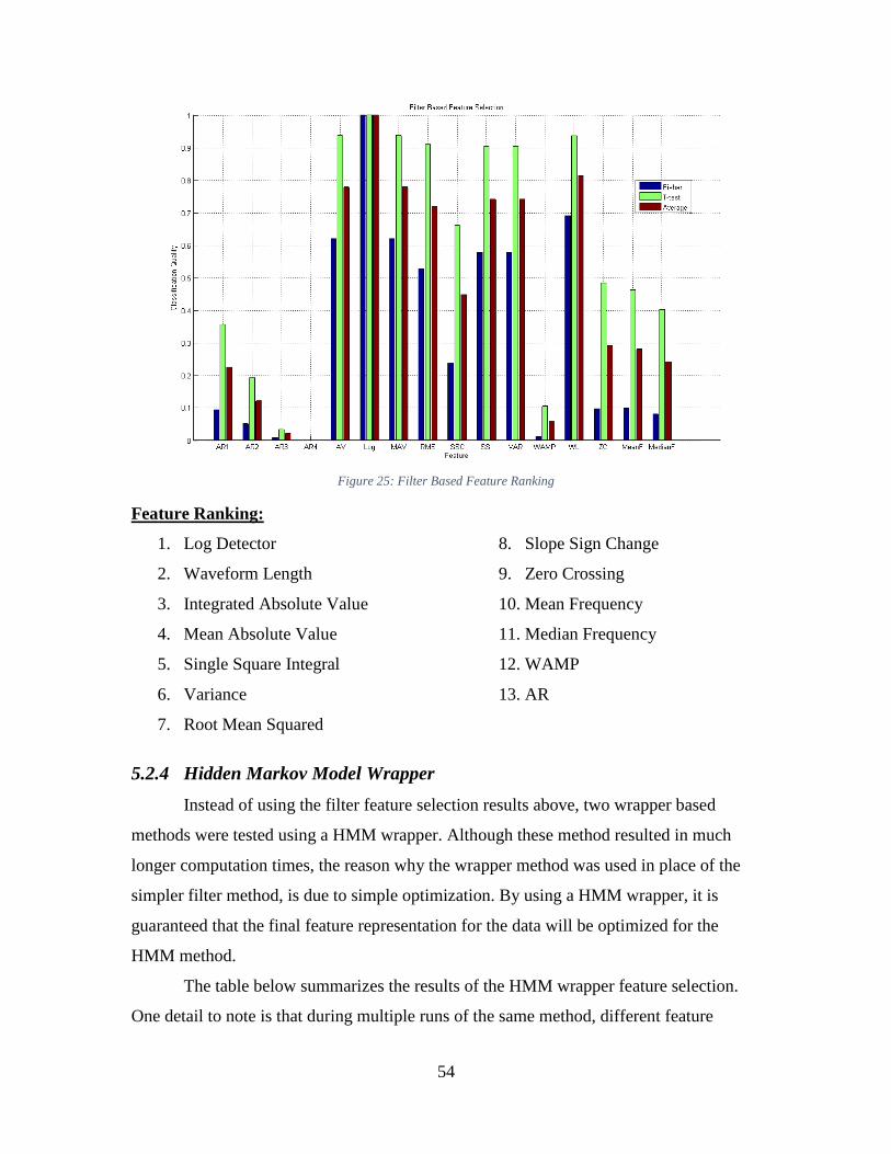
54
Figure 25: Filter Based Feature Ranking
Feature Ranking:
1. Log Detector
2. Waveform Length
3. Integrated Absolute Value
4. Mean Absolute Value
5. Single Square Integral
6. Variance
7. Root Mean Squared
8. Slope Sign Change
9. Zero Crossing
10. Mean Frequency
11. Median Frequency
12. WAMP
13. AR
5.2.4 Hidden Markov Model Wrapper
Instead of using the filter feature selection results above, two wrapper based
methods were tested using a HMM wrapper. Although these method resulted in much
longer computation times, the reason why the wrapper method was used in place of the
simpler filter method, is due to simple optimization. By using a HMM wrapper, it is
guaranteed that the final feature representation for the data will be optimized for the
HMM method.
The table below summarizes the results of the HMM wrapper feature selection.
One detail to note is that during multiple runs of the same method, different feature
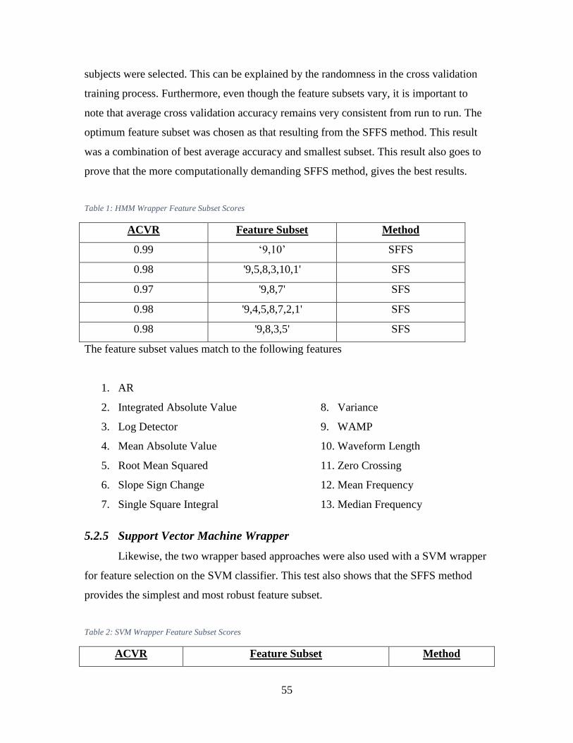
55
subjects were selected. This can be explained by the randomness in the cross validation
training process. Furthermore, even though the feature subsets vary, it is important to
note that average cross validation accuracy remains very consistent from run to run. The
optimum feature subset was chosen as that resulting from the SFFS method. This result
was a combination of best average accuracy and smallest subset. This result also goes to
prove that the more computationally demanding SFFS method, gives the best results.
Table 1: HMM Wrapper Feature Subset Scores
ACVR Feature Subset Method
0.99 ‘9,10’ SFFS
0.98 '9,5,8,3,10,1' SFS
0.97 '9,8,7' SFS
0.98 '9,4,5,8,7,2,1' SFS
0.98 '9,8,3,5' SFS
The feature subset values match to the following features
1. AR
2. Integrated Absolute Value
3. Log Detector
4. Mean Absolute Value
5. Root Mean Squared
6. Slope Sign Change
7. Single Square Integral
8. Variance
9. WAMP
10. Waveform Length
11. Zero Crossing
12. Mean Frequency
13. Median Frequency
5.2.5 Support Vector Machine Wrapper
Likewise, the two wrapper based approaches were also used with a SVM wrapper
for feature selection on the SVM classifier. This test also shows that the SFFS method
provides the simplest and most robust feature subset.
Table 2: SVM Wrapper Feature Subset Scores
ACVR Feature Subset Method
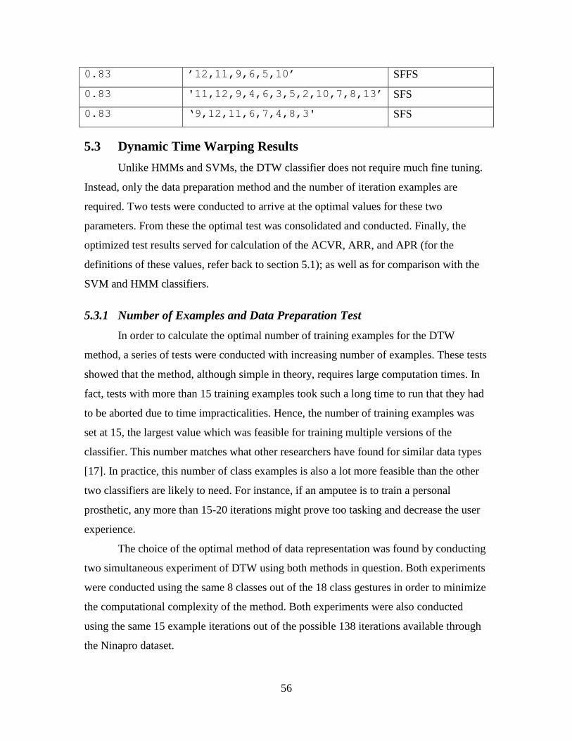
56
0.83 ’12,11,9,6,5,10’ SFFS
0.83 '11,12,9,4,6,3,5,2,10,7,8,13’ SFS
0.83 ‘9,12,11,6,7,4,8,3' SFS
5.3 Dynamic Time Warping Results
Unlike HMMs and SVMs, the DTW classifier does not require much fine tuning.
Instead, only the data preparation method and the number of iteration examples are
required. Two tests were conducted to arrive at the optimal values for these two
parameters. From these the optimal test was consolidated and conducted. Finally, the
optimized test results served for calculation of the ACVR, ARR, and APR (for the
definitions of these values, refer back to section 5.1); as well as for comparison with the
SVM and HMM classifiers.
5.3.1 Number of Examples and Data Preparation Test
In order to calculate the optimal number of training examples for the DTW
method, a series of tests were conducted with increasing number of examples. These tests
showed that the method, although simple in theory, requires large computation times. In
fact, tests with more than 15 training examples took such a long time to run that they had
to be aborted due to time impracticalities. Hence, the number of training examples was
set at 15, the largest value which was feasible for training multiple versions of the
classifier. This number matches what other researchers have found for similar data types
[17]. In practice, this number of class examples is also a lot more feasible than the other
two classifiers are likely to need. For instance, if an amputee is to train a personal
prosthetic, any more than 15-20 iterations might prove too tasking and decrease the user
experience.
The choice of the optimal method of data representation was found by conducting
two simultaneous experiment of DTW using both methods in question. Both experiments
were conducted using the same 8 classes out of the 18 class gestures in order to minimize
the computational complexity of the method. Both experiments were also conducted
using the same 15 example iterations out of the possible 138 iterations available through
the Ninapro dataset.
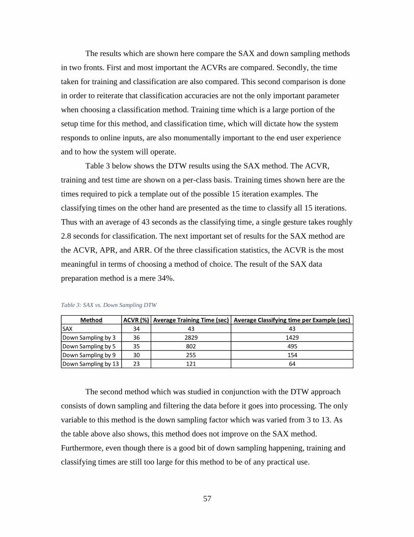
57
The results which are shown here compare the SAX and down sampling methods
in two fronts. First and most important the ACVRs are compared. Secondly, the time
taken for training and classification are also compared. This second comparison is done
in order to reiterate that classification accuracies are not the only important parameter
when choosing a classification method. Training time which is a large portion of the
setup time for this method, and classification time, which will dictate how the system
responds to online inputs, are also monumentally important to the end user experience
and to how the system will operate.
Table 3 below shows the DTW results using the SAX method. The ACVR,
training and test time are shown on a per-class basis. Training times shown here are the
times required to pick a template out of the possible 15 iteration examples. The
classifying times on the other hand are presented as the time to classify all 15 iterations.
Thus with an average of 43 seconds as the classifying time, a single gesture takes roughly
2.8 seconds for classification. The next important set of results for the SAX method are
the ACVR, APR, and ARR. Of the three classification statistics, the ACVR is the most
meaningful in terms of choosing a method of choice. The result of the SAX data
preparation method is a mere 34%.
Table 3: SAX vs. Down Sampling DTW
The second method which was studied in conjunction with the DTW approach
consists of down sampling and filtering the data before it goes into processing. The only
variable to this method is the down sampling factor which was varied from 3 to 13. As
the table above also shows, this method does not improve on the SAX method.
Furthermore, even though there is a good bit of down sampling happening, training and
classifying times are still too large for this method to be of any practical use.
Method ACVR (%) Average Training Time (sec) Average Classifying time per Example (sec)
SAX 34 43 43
Down Sampling by 3 36 2829 1429
Down Sampling by 5 35 802 495
Down Sampling by 9 30 255 154
Down Sampling by 13 23 121 64
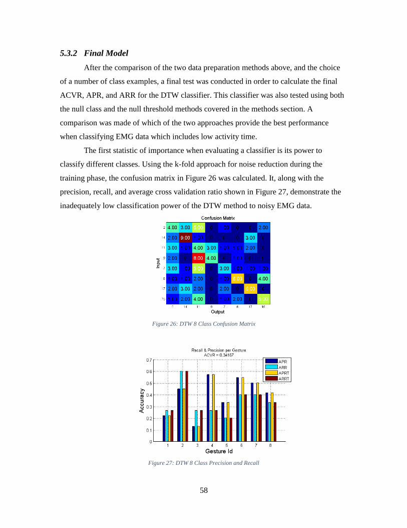
58
5.3.2 Final Model
After the comparison of the two data preparation methods above, and the choice
of a number of class examples, a final test was conducted in order to calculate the final
ACVR, APR, and ARR for the DTW classifier. This classifier was also tested using both
the null class and the null threshold methods covered in the methods section. A
comparison was made of which of the two approaches provide the best performance
when classifying EMG data which includes low activity time.
The first statistic of importance when evaluating a classifier is its power to
classify different classes. Using the k-fold approach for noise reduction during the
training phase, the confusion matrix in Figure 26 was calculated. It, along with the
precision, recall, and average cross validation ratio shown in Figure 27, demonstrate the
inadequately low classification power of the DTW method to noisy EMG data.
Figure 26: DTW 8 Class Confusion Matrix
Figure 27: DTW 8 Class Precision and Recall
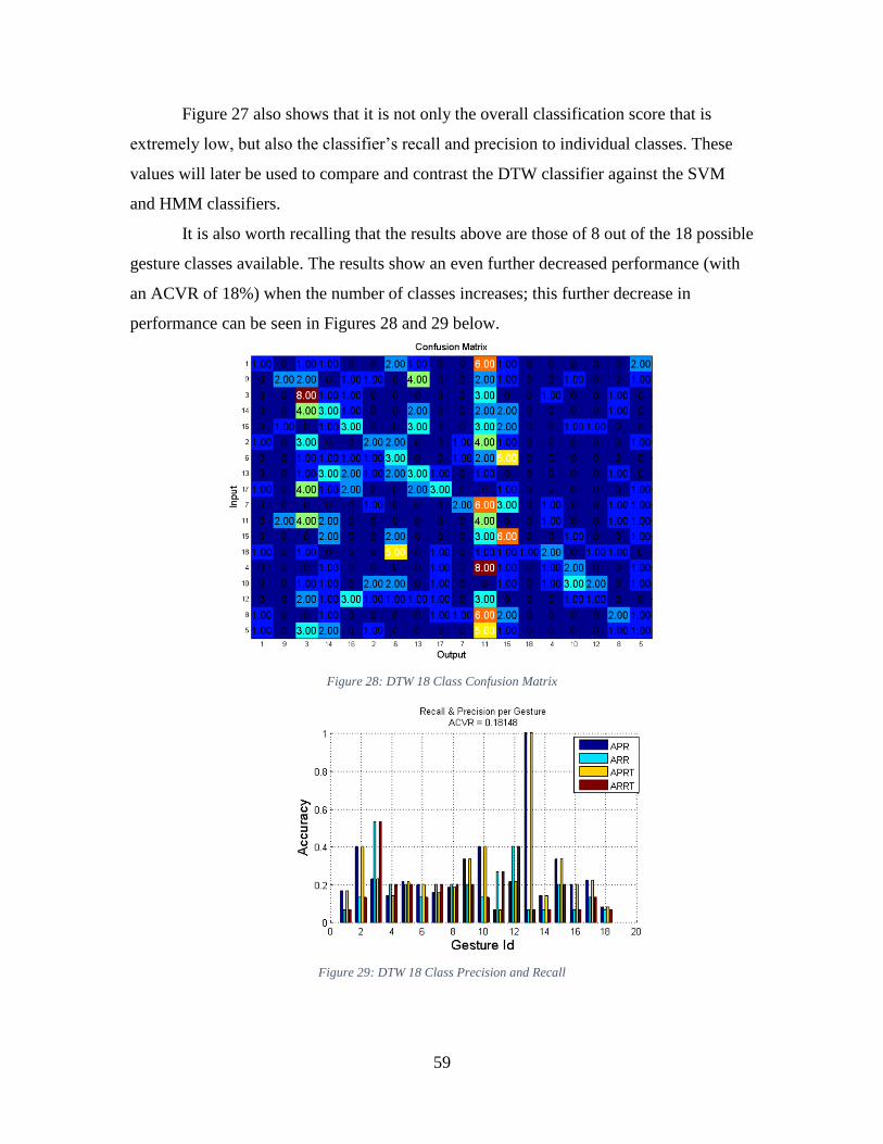
59
Figure 27 also shows that it is not only the overall classification score that is
extremely low, but also the classifier’s recall and precision to individual classes. These
values will later be used to compare and contrast the DTW classifier against the SVM
and HMM classifiers.
It is also worth recalling that the results above are those of 8 out of the 18 possible
gesture classes available. The results show an even further decreased performance (with
an ACVR of 18%) when the number of classes increases; this further decrease in
performance can be seen in Figures 28 and 29 below.
Figure 28: DTW 18 Class Confusion Matrix
Figure 29: DTW 18 Class Precision and Recall
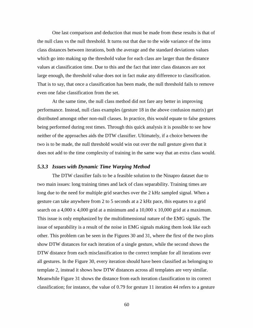
60
One last comparison and deduction that must be made from these results is that of
the null class vs the null threshold. It turns out that due to the wide variance of the intra
class distances between iterations, both the average and the standard deviations values
which go into making up the threshold value for each class are larger than the distance
values at classification time. Due to this and the fact that inter class distances are not
large enough, the threshold value does not in fact make any difference to classification.
That is to say, that once a classification has been made, the null threshold fails to remove
even one false classification from the set.
At the same time, the null class method did not fare any better in improving
performance. Instead, null class examples (gesture 18 in the above confusion matrix) get
distributed amongst other non-null classes. In practice, this would equate to false gestures
being performed during rest times. Through this quick analysis it is possible to see how
neither of the approaches aids the DTW classifier. Ultimately, if a choice between the
two is to be made, the null threshold would win out over the null gesture given that it
does not add to the time complexity of training in the same way that an extra class would.
5.3.3 Issues with Dynamic Time Warping Method
The DTW classifier fails to be a feasible solution to the Ninapro dataset due to
two main issues: long training times and lack of class separability. Training times are
long due to the need for multiple grid searches over the 2 kHz sampled signal. When a
gesture can take anywhere from 2 to 5 seconds at a 2 kHz pace, this equates to a grid
search on a 4,000 x 4,000 grid at a minimum and a 10,000 x 10,000 grid at a maximum.
This issue is only emphasized by the multidimensional nature of the EMG signals. The
issue of separability is a result of the noise in EMG signals making them look like each
other. This problem can be seen in the Figures 30 and 31, where the first of the two plots
show DTW distances for each iteration of a single gesture, while the second shows the
DTW distance from each misclassification to the correct template for all iterations over
all gestures. In the Figure 30, every iteration should have been classified as belonging to
template 2, instead it shows how DTW distances across all templates are very similar.
Meanwhile Figure 31 shows the distance from each iteration classification to its correct
classification; for instance, the value of 0.79 for gesture 11 iteration 44 refers to a gesture
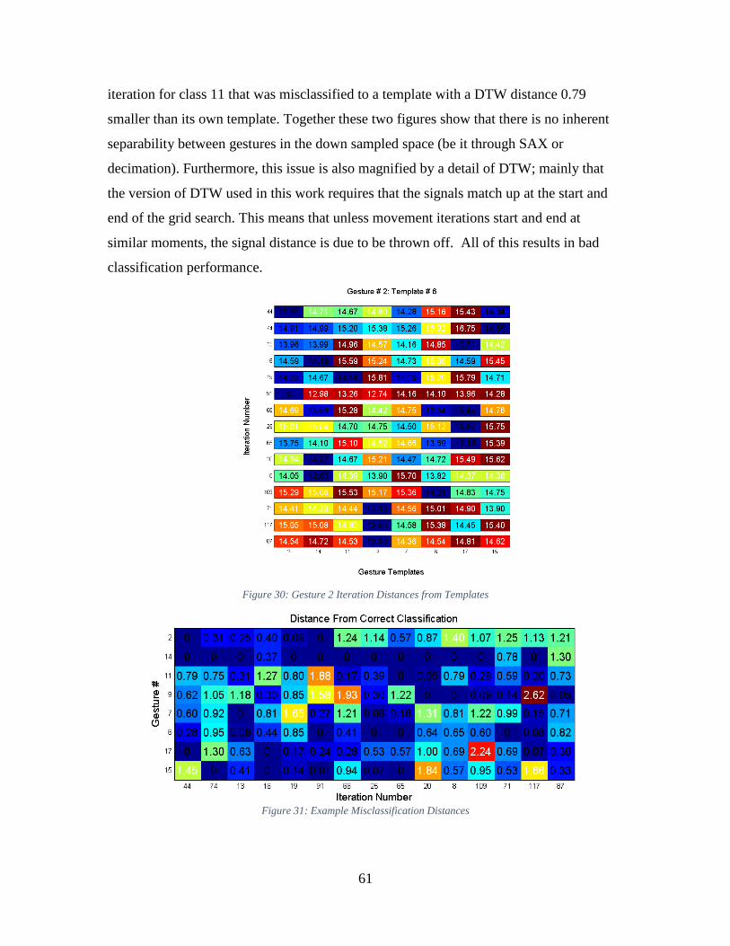
61
iteration for class 11 that was misclassified to a template with a DTW distance 0.79
smaller than its own template. Together these two figures show that there is no inherent
separability between gestures in the down sampled space (be it through SAX or
decimation). Furthermore, this issue is also magnified by a detail of DTW; mainly that
the version of DTW used in this work requires that the signals match up at the start and
end of the grid search. This means that unless movement iterations start and end at
similar moments, the signal distance is due to be thrown off. All of this results in bad
classification performance.
Figure 30: Gesture 2 Iteration Distances from Templates
Figure 31: Example Misclassification Distances

62
A solution to the first issue might be to down sample to data, however, this was
studied in the previous section and found not to produce reliable performance. The reason
for this might be that down sampling was done through decimation. This might also be a
reason why the SAX method performed better than down sampling, since it ‘down
samples’ in a smart way. As for the second problem, a version of DTW might be
presented in which the requirement for a full data grid is relaxed. This might create more
cohesion between class members while distinguishing different classes.
5.4 Hidden Markov Model Results
In order to set the optimal parameters for the HMM gesture classifier, the
following experiments were conducted. Each test is designed to optimize one HMM
parameter. The first, finds the optimal number of states and emission observations for the
model. The second tests the assumption that left to right models are optimal when
compared to ergodic models. The third and fourth test for the classifier’s power to
distinguish between a range of classes, and the minimum amount of information required
for training. Finally, all these tests are combined and tested in unison. The SAX
discretization approach is also tested and compared to the feature extraction approach.
5.4.1 Model Setup
The first test conducted for the HMM classifier aims to find the optimal number
of states and observations for the model. In the case of gestures, a state in a HMM could
also be considered the step during a movement sequence, while an observation is the
EMG data that is collected by the sensors and recorded.
This test while only the first one conducted specifically for HMM, is also one of
the most important. The importance of these two parameters can be seen in Figure 32,
which shows the average cross validation results for the grid search conducted.
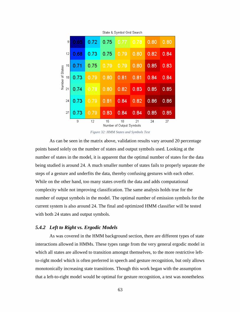
63
Figure 32: HMM States and Symbols Test
As can be seen in the matrix above, validation results vary around 20 percentage
points based solely on the number of states and output symbols used. Looking at the
number of states in the model, it is apparent that the optimal number of states for the data
being studied is around 24. A much smaller number of states fails to properly separate the
steps of a gesture and underfits the data, thereby confusing gestures with each other.
While on the other hand, too many states overfit the data and adds computational
complexity while not improving classification. The same analysis holds true for the
number of output symbols in the model. The optimal number of emission symbols for the
current system is also around 24. The final and optimized HMM classifier will be tested
with both 24 states and output symbols.
5.4.2 Left to Right vs. Ergodic Models
As was covered in the HMM background section, there are different types of state
interactions allowed in HMMs. These types range from the very general ergodic model in
which all states are allowed to transition amongst themselves, to the more restrictive left-
to-right model which is often preferred in speech and gesture recognition, but only allows
monotonically increasing state transitions. Though this work began with the assumption
that a left-to-right model would be optimal for gesture recognition, a test was nonetheless
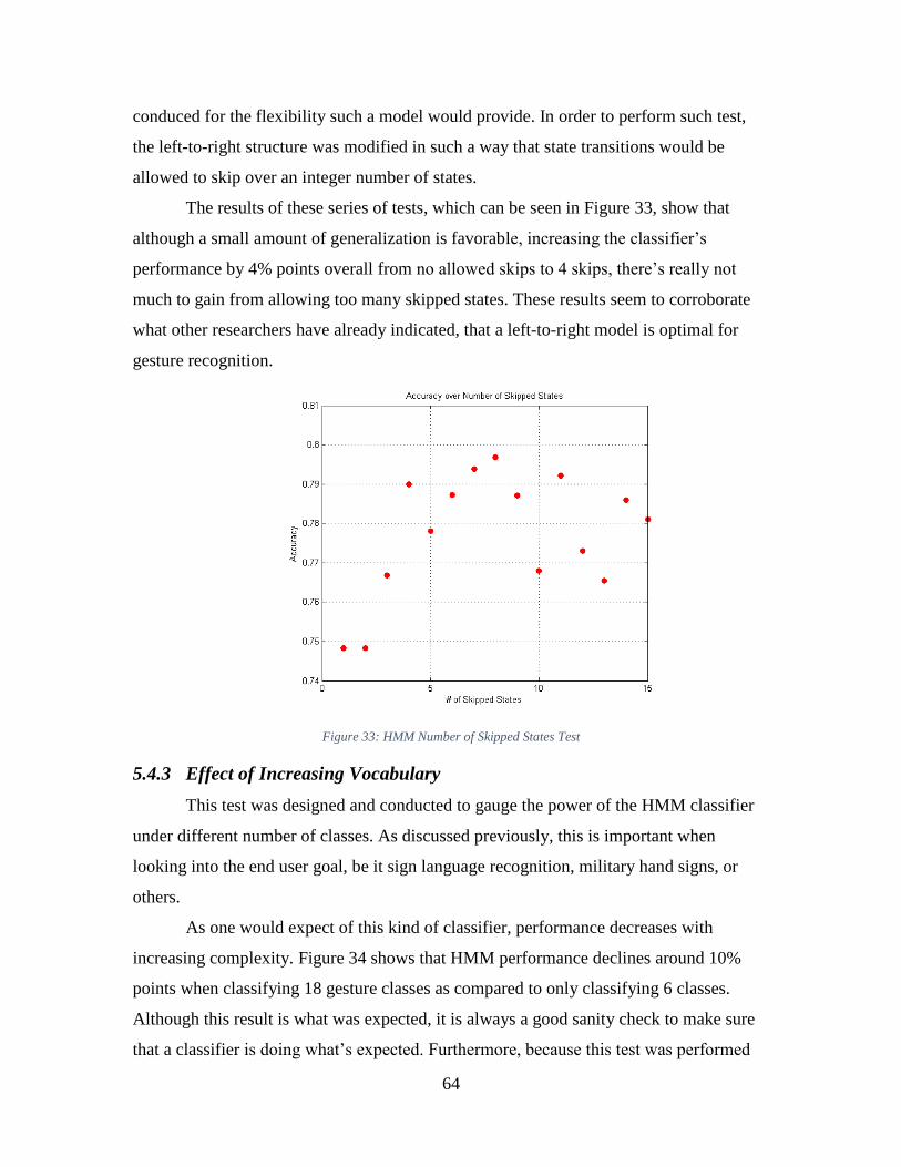
64
conduced for the flexibility such a model would provide. In order to perform such test,
the left-to-right structure was modified in such a way that state transitions would be
allowed to skip over an integer number of states.
The results of these series of tests, which can be seen in Figure 33, show that
although a small amount of generalization is favorable, increasing the classifier’s
performance by 4% points overall from no allowed skips to 4 skips, there’s really not
much to gain from allowing too many skipped states. These results seem to corroborate
what other researchers have already indicated, that a left-to-right model is optimal for
gesture recognition.
Figure 33: HMM Number of Skipped States Test
5.4.3 Effect of Increasing Vocabulary
This test was designed and conducted to gauge the power of the HMM classifier
under different number of classes. As discussed previously, this is important when
looking into the end user goal, be it sign language recognition, military hand signs, or
others.
As one would expect of this kind of classifier, performance decreases with
increasing complexity. Figure 34 shows that HMM performance declines around 10%
points when classifying 18 gesture classes as compared to only classifying 6 classes.
Although this result is what was expected, it is always a good sanity check to make sure
that a classifier is doing what’s expected. Furthermore, because this test was performed

65
with a number of variations, the results also go to show something that has already been
proven, that a 24 state model outperforms a 15 state model in average cross validation.
Figure 34: HMM Accuracy Over Number of Classes
5.4.4 Minimum Required Training Data
The following test was performed for estimating a minimum number of training
observation required for proper HMM operation. Previous works have hinted at around
70 training observations being necessary for training a Hidden Markov model. This
number is consistent with the outcomes of this test, which are depicted below.
As can be seen, a HMM’s performance rapidly increases at small amounts of
training data; increasing the training set from 10 to 20 observations increases
performance by roughly 15% points, and adding another 20 training instances, adds
another 15% points. However, this rate of increased performance is not consistent when
adding more data samples. Instead, the learning curve reaches a semi plateau at around 80
training samples, where much more data improves the classifier’s performance in a
disproportionate rate to the of growth in computational complexity.
Figure 35 shows results for a number of runs of the HMM classifier under
different conditions. These conditions vary not only in the number of training samples,
but also the representation of the data, the feature subset, the number of states and
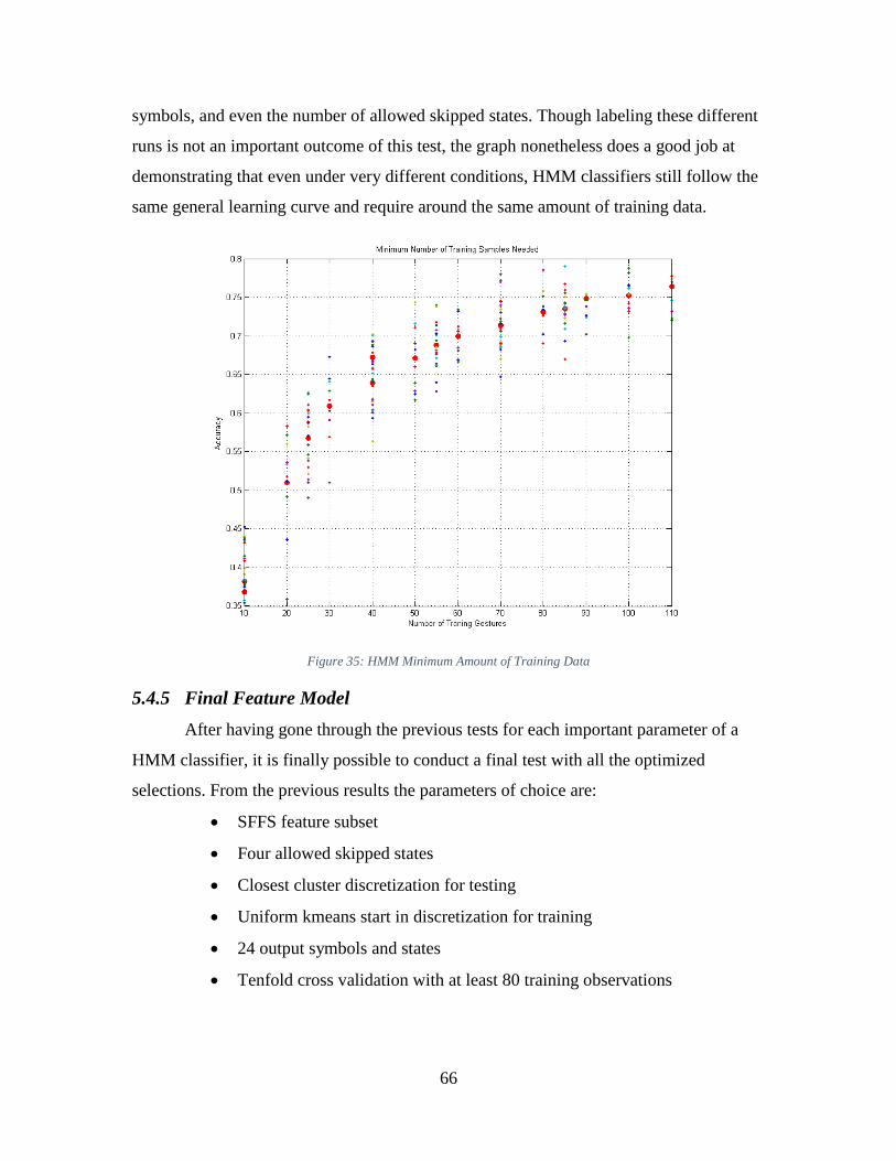
66
symbols, and even the number of allowed skipped states. Though labeling these different
runs is not an important outcome of this test, the graph nonetheless does a good job at
demonstrating that even under very different conditions, HMM classifiers still follow the
same general learning curve and require around the same amount of training data.
Figure 35: HMM Minimum Amount of Training Data
5.4.5 Final Feature Model
After having gone through the previous tests for each important parameter of a
HMM classifier, it is finally possible to conduct a final test with all the optimized
selections. From the previous results the parameters of choice are:
SFFS feature subset
Four allowed skipped states
Closest cluster discretization for testing
Uniform kmeans start in discretization for training
24 output symbols and states
Tenfold cross validation with at least 80 training observations
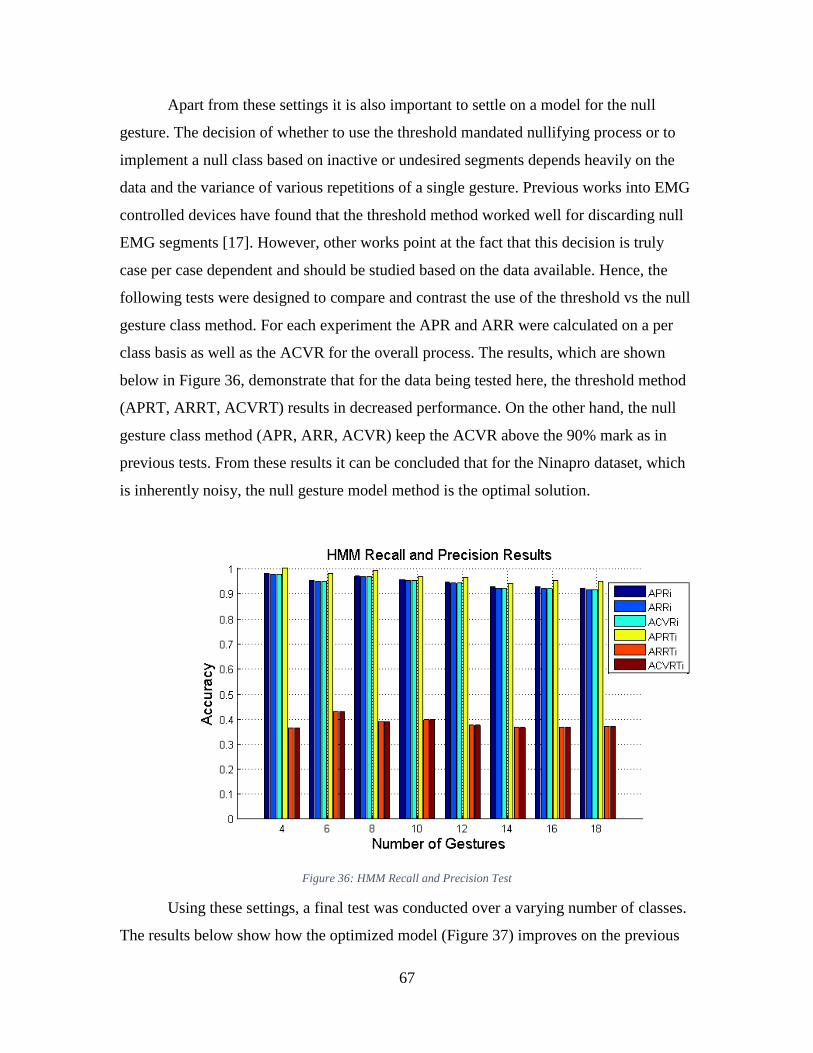
67
Apart from these settings it is also important to settle on a model for the null
gesture. The decision of whether to use the threshold mandated nullifying process or to
implement a null class based on inactive or undesired segments depends heavily on the
data and the variance of various repetitions of a single gesture. Previous works into EMG
controlled devices have found that the threshold method worked well for discarding null
EMG segments [17]. However, other works point at the fact that this decision is truly
case per case dependent and should be studied based on the data available. Hence, the
following tests were designed to compare and contrast the use of the threshold vs the null
gesture class method. For each experiment the APR and ARR were calculated on a per
class basis as well as the ACVR for the overall process. The results, which are shown
below in Figure 36, demonstrate that for the data being tested here, the threshold method
(APRT, ARRT, ACVRT) results in decreased performance. On the other hand, the null
gesture class method (APR, ARR, ACVR) keep the ACVR above the 90% mark as in
previous tests. From these results it can be concluded that for the Ninapro dataset, which
is inherently noisy, the null gesture model method is the optimal solution.
Figure 36: HMM Recall and Precision Test
Using these settings, a final test was conducted over a varying number of classes.
The results below show how the optimized model (Figure 37) improves on the previous
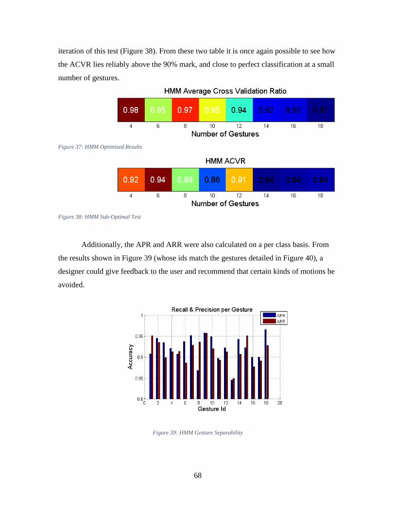
68
iteration of this test (Figure 38). From these two table it is once again possible to see how
the ACVR lies reliably above the 90% mark, and close to perfect classification at a small
number of gestures.
Figure 37: HMM Optimized Results
Figure 38: HMM Sub-Optimal Test
Additionally, the APR and ARR were also calculated on a per class basis. From
the results shown in Figure 39 (whose ids match the gestures detailed in Figure 40), a
designer could give feedback to the user and recommend that certain kinds of motions be
avoided.
Figure 39: HMM Gesture Separability
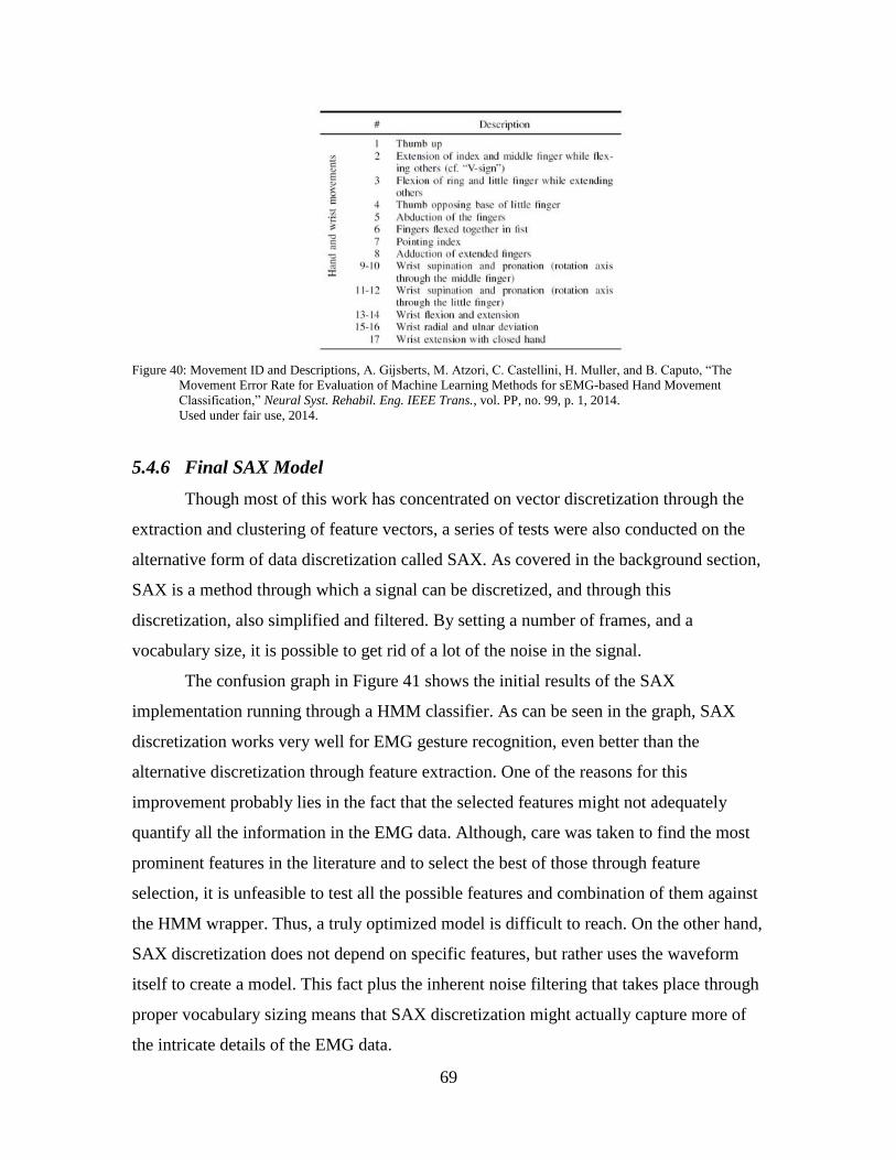
69
Figure 40: Movement ID and Descriptions, A. Gijsberts, M. Atzori, C. Castellini, H. Muller, and B. Caputo, “The
Movement Error Rate for Evaluation of Machine Learning Methods for sEMG-based Hand Movement
Classification,” Neural Syst. Rehabil. Eng. IEEE Trans., vol. PP, no. 99, p. 1, 2014.
Used under fair use, 2014.
5.4.6 Final SAX Model
Though most of this work has concentrated on vector discretization through the
extraction and clustering of feature vectors, a series of tests were also conducted on the
alternative form of data discretization called SAX. As covered in the background section,
SAX is a method through which a signal can be discretized, and through this
discretization, also simplified and filtered. By setting a number of frames, and a
vocabulary size, it is possible to get rid of a lot of the noise in the signal.
The confusion graph in Figure 41 shows the initial results of the SAX
implementation running through a HMM classifier. As can be seen in the graph, SAX
discretization works very well for EMG gesture recognition, even better than the
alternative discretization through feature extraction. One of the reasons for this
improvement probably lies in the fact that the selected features might not adequately
quantify all the information in the EMG data. Although, care was taken to find the most
prominent features in the literature and to select the best of those through feature
selection, it is unfeasible to test all the possible features and combination of them against
the HMM wrapper. Thus, a truly optimized model is difficult to reach. On the other hand,
SAX discretization does not depend on specific features, but rather uses the waveform
itself to create a model. This fact plus the inherent noise filtering that takes place through
proper vocabulary sizing means that SAX discretization might actually capture more of
the intricate details of the EMG data.
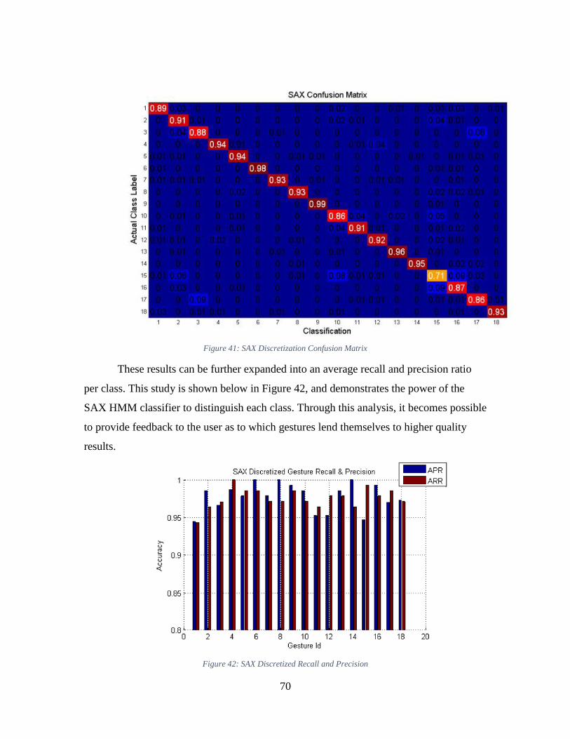
70
Figure 41: SAX Discretization Confusion Matrix
These results can be further expanded into an average recall and precision ratio
per class. This study is shown below in Figure 42, and demonstrates the power of the
SAX HMM classifier to distinguish each class. Through this analysis, it becomes possible
to provide feedback to the user as to which gestures lend themselves to higher quality
results.
Figure 42: SAX Discretized Recall and Precision
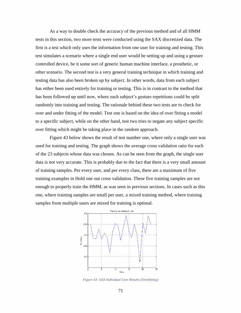
71
As a way to double check the accuracy of the previous method and of all HMM
tests in this section, two more tests were conducted using the SAX discretized data. The
first is a test which only uses the information from one user for training and testing. This
test simulates a scenario where a single end user would be setting up and using a gesture
controlled device, be it some sort of generic human machine interface, a prosthetic, or
other scenario. The second test is a very general training technique in which training and
testing data has also been broken up by subject. In other words, data from each subject
has either been used entirely for training or testing. This is in contrast to the method that
has been followed up until now, where each subject’s gesture repetitions could be split
randomly into training and testing. The rationale behind these two tests are to check for
over and under fitting of the model. Test one is based on the idea of over fitting a model
to a specific subject, while on the other hand, test two tries to negate any subject specific
over fitting which might be taking place in the random approach.
Figure 43 below shows the result of test number one, where only a single user was
used for training and testing. The graph shows the average cross validation ratio for each
of the 23 subjects whose data was chosen. As can be seen from the graph, the single user
data is not very accurate. This is probably due to the fact that there is a very small amount
of training samples. Per every user, and per every class, there are a maximum of five
training examples in Hold one out cross validation. These five training samples are not
enough to properly train the HMM, as was seen in previous sections. In cases such as this
one, where training samples are small per user, a mixed training method, where training
samples from multiple users are mixed for training is optimal.
Figure 43: SAX Individual User Results (Overfitting)
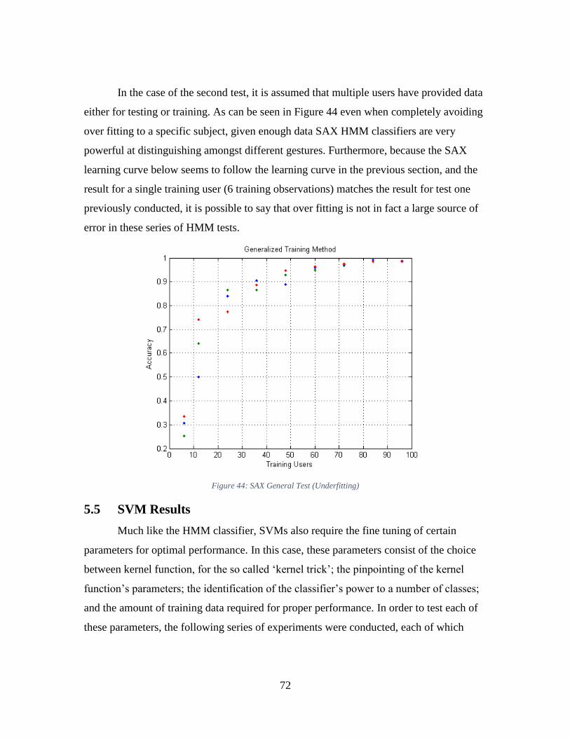
72
In the case of the second test, it is assumed that multiple users have provided data
either for testing or training. As can be seen in Figure 44 even when completely avoiding
over fitting to a specific subject, given enough data SAX HMM classifiers are very
powerful at distinguishing amongst different gestures. Furthermore, because the SAX
learning curve below seems to follow the learning curve in the previous section, and the
result for a single training user (6 training observations) matches the result for test one
previously conducted, it is possible to say that over fitting is not in fact a large source of
error in these series of HMM tests.
Figure 44: SAX General Test (Underfitting)
5.5 SVM Results
Much like the HMM classifier, SVMs also require the fine tuning of certain
parameters for optimal performance. In this case, these parameters consist of the choice
between kernel function, for the so called ‘kernel trick’; the pinpointing of the kernel
function’s parameters; the identification of the classifier’s power to a number of classes;
and the amount of training data required for proper performance. In order to test each of
these parameters, the following series of experiments were conducted, each of which
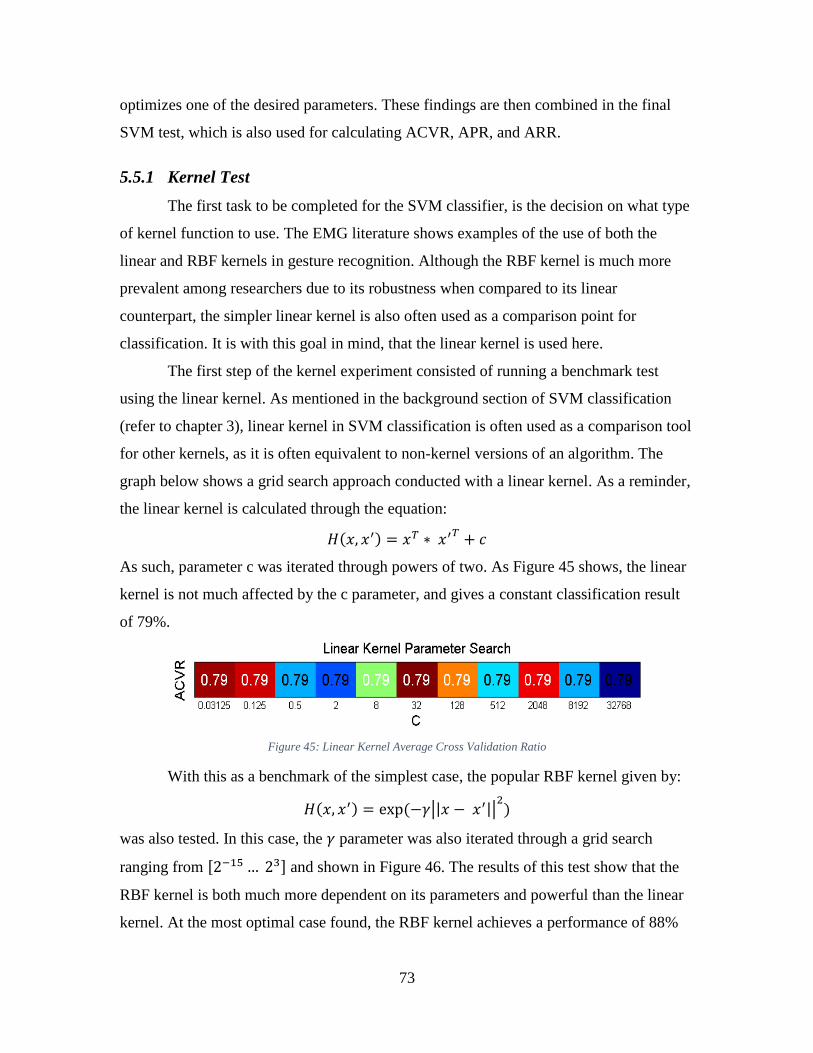
73
optimizes one of the desired parameters. These findings are then combined in the final
SVM test, which is also used for calculating ACVR, APR, and ARR.
5.5.1 Kernel Test
The first task to be completed for the SVM classifier, is the decision on what type
of kernel function to use. The EMG literature shows examples of the use of both the
linear and RBF kernels in gesture recognition. Although the RBF kernel is much more
prevalent among researchers due to its robustness when compared to its linear
counterpart, the simpler linear kernel is also often used as a comparison point for
classification. It is with this goal in mind, that the linear kernel is used here.
The first step of the kernel experiment consisted of running a benchmark test
using the linear kernel. As mentioned in the background section of SVM classification
(refer to chapter 3), linear kernel in SVM classification is often used as a comparison tool
for other kernels, as it is often equivalent to non-kernel versions of an algorithm. The
graph below shows a grid search approach conducted with a linear kernel. As a reminder,
the linear kernel is calculated through the equation:
As such, parameter c was iterated through powers of two. As Figure 45 shows, the linear
kernel is not much affected by the c parameter, and gives a constant classification result
of 79%.
Figure 45: Linear Kernel Average Cross Validation Ratio
With this as a benchmark of the simplest case, the popular RBF kernel given by:
| |
was also tested. In this case, the parameter was also iterated through a grid search
ranging from and shown in Figure 46. The results of this test show that the
RBF kernel is both much more dependent on its parameters and powerful than the linear
kernel. At the most optimal case found, the RBF kernel achieves a performance of 88%
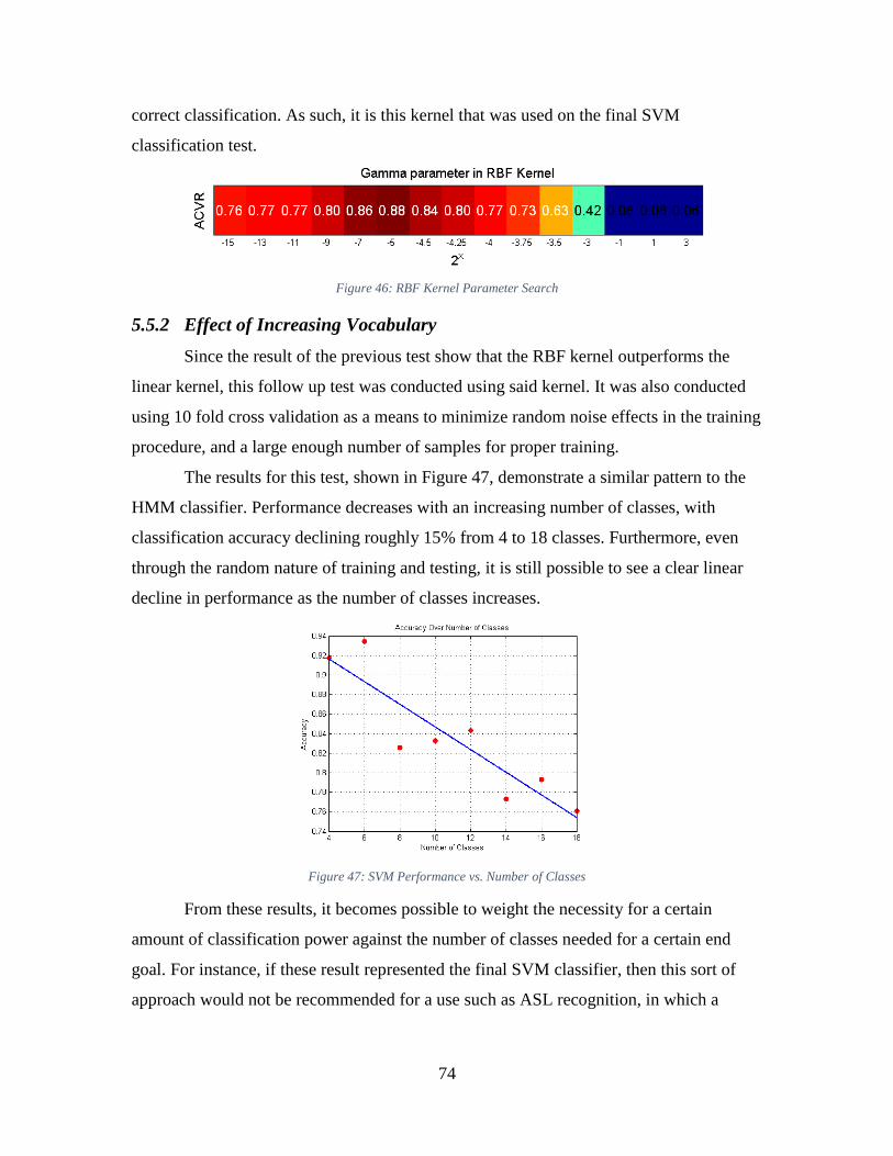
74
correct classification. As such, it is this kernel that was used on the final SVM
classification test.
Figure 46: RBF Kernel Parameter Search
5.5.2 Effect of Increasing Vocabulary
Since the result of the previous test show that the RBF kernel outperforms the
linear kernel, this follow up test was conducted using said kernel. It was also conducted
using 10 fold cross validation as a means to minimize random noise effects in the training
procedure, and a large enough number of samples for proper training.
The results for this test, shown in Figure 47, demonstrate a similar pattern to the
HMM classifier. Performance decreases with an increasing number of classes, with
classification accuracy declining roughly 15% from 4 to 18 classes. Furthermore, even
through the random nature of training and testing, it is still possible to see a clear linear
decline in performance as the number of classes increases.
Figure 47: SVM Performance vs. Number of Classes
From these results, it becomes possible to weight the necessity for a certain
amount of classification power against the number of classes needed for a certain end
goal. For instance, if these result represented the final SVM classifier, then this sort of
approach would not be recommended for a use such as ASL recognition, in which a
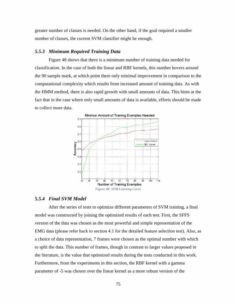
75
greater number of classes is needed. On the other hand, if the goal required a smaller
number of classes, the current SVM classifier might be enough.
5.5.3 Minimum Required Training Data
Figure 48 shows that there is a minimum number of training data needed for
classification. In the case of both the linear and RBF kernels, this number hovers around
the 90 sample mark, at which point there only minimal improvement in comparison to the
computational complexity which results from increased amount of training data. As with
the HMM method, there is also rapid growth with small amounts of data. This hints at the
fact that in the case where only small amounts of data is available, efforts should be made
to collect more data.
Figure 48: SVM Learning Curve
5.5.4 Final SVM Model
After the series of tests to optimize different parameters of SVM training, a final
model was constructed by joining the optimized results of each test. First, the SFFS
version of the data was chosen as the most powerful and simple representation of the
EMG data (please refer back to section 4.1 for the detailed feature selection test). Also, as
a choice of data representation, 7 frames were chosen as the optimal number with which
to split the data. This number of frames, though in contrast to larger values proposed in
the literature, is the value that optimized results during the tests conducted in this work.
Furthermore, from the experiments in this section, the RBF kernel with a gamma
parameter of -5 was chosen over the linear kernel as a more robust version of the
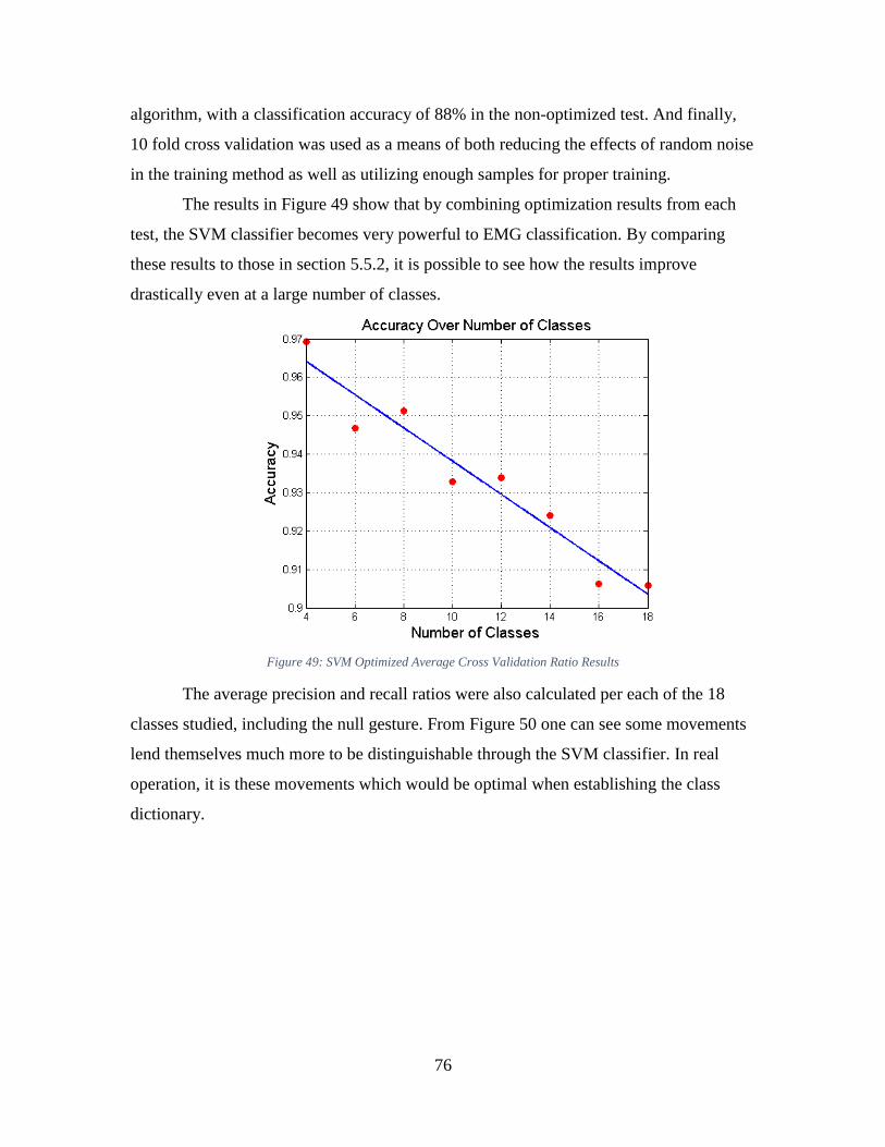
76
algorithm, with a classification accuracy of 88% in the non-optimized test. And finally,
10 fold cross validation was used as a means of both reducing the effects of random noise
in the training method as well as utilizing enough samples for proper training.
The results in Figure 49 show that by combining optimization results from each
test, the SVM classifier becomes very powerful to EMG classification. By comparing
these results to those in section 5.5.2, it is possible to see how the results improve
drastically even at a large number of classes.
Figure 49: SVM Optimized Average Cross Validation Ratio Results
The average precision and recall ratios were also calculated per each of the 18
classes studied, including the null gesture. From Figure 50 one can see some movements
lend themselves much more to be distinguishable through the SVM classifier. In real
operation, it is these movements which would be optimal when establishing the class
dictionary.
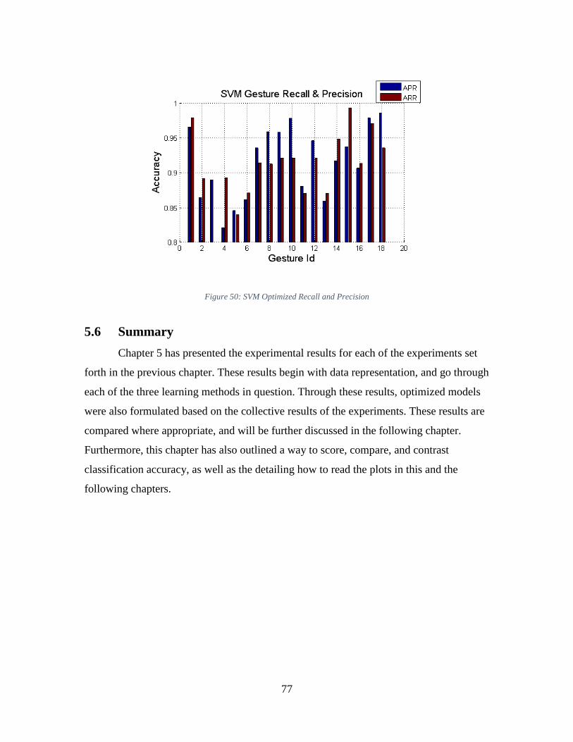
77
Figure 50: SVM Optimized Recall and Precision
5.6 Summary
Chapter 5 has presented the experimental results for each of the experiments set
forth in the previous chapter. These results begin with data representation, and go through
each of the three learning methods in question. Through these results, optimized models
were also formulated based on the collective results of the experiments. These results are
compared where appropriate, and will be further discussed in the following chapter.
Furthermore, this chapter has also outlined a way to score, compare, and contrast
classification accuracy, as well as the detailing how to read the plots in this and the
following chapters.

78
6 Conclusions
6.1 Chapter Summary
After reviewing all test results, it is possible to go back and interpret them in the
context of the initial problem formulation. This thesis deals with the comparison of three
distinct classifiers for human gesture recognition and their optimization for the Ninapro
dataset. This dataset is a new benchmarking tool which continues to gain traction
amongst gesture classification researcher for comparison of different tactics. As such this
chapter will first cover the results offered by other researchers with the same dataset, then
it will compare the three classifiers chosen for optimal operation, it will cover the final
achievement towards gesture classification, and finally will cover future work which
might result from this analysis.
6.2 Previous Ninapro Results
The Ninapro dataset is quickly becoming popular as a tool for comparison. Since
its latest version was released in 2014 with the work entitled “Characterization of a
Benchmark Database for Myoelectric Movement Classification”, multiple researchers
have applied a number of classification tools to the set and reported their results [49].
Although not a comprehensive list, the results taken from the Ninapro website are
detailed below. These results show a sample of the different approaches taken by
researchers, mainly the use of k-nearest neighbors and linear discriminant analysis. The
table also shows that thus far, of the classification results available through the Ninapro
website, the maximum efficiency achieved has been 83.5%. These results will be used
for comparison of the classifiers used in this work.
Table 4: Ninapro Classification Results
For the three classifiers tested here, there are two important aspects which must be
explored. The first consists of the time required for training and classification using each
Classification Mode Procedure Movements Classification Results (%)
Intra Subject Custom Acquisition Procedure All, rest included 83.5
Intra Subject k-nn All, rest included 55
Intra Subject multi k-nn All, without rest 50
Intra Subject multi k-nn All, without rest 52
Intra Subject LDA All, without rest 40
79
method. This parameter is important for two reasons; first, during development time
when multiple methods and versions must be tested, long training times would be
inefficient and reduce the number of possible test iterations, thereby reducing the possible
scenario searchers and possibly occluding the optimal result. Secondly, after a system has
been deployed for consumer use, classification times will mandate the time the system
requires to make a classification, which in turn will mandate the responsiveness of the
system and its ease of use for the subject. The second parameter which will be explored is
the system’s classification accuracy. These results are obviously important given that low
accuracies demonstrate the inability of the algorithm to recognize a gesture.
6.3 Thesis Results
First, let’s take a look at training and classification times for the three classifiers.
Figures 51-53 below demonstrate the performance of the SVM, HMM, and DTW
methods respectively. Due to the time complexity of each method, the results for both the
SVM and HMM classifier are shown as an average over a number of different gestures
from 4 to 18 gesture classes; however, for the DTW method which required the most
training time, results are shown are only for the 8 class set. In order to compare the three
outcomes, it is necessary to compare the SVM and HMM 8 class gesture result, with the
DTW result. These times immediately show how although both the SVM and HMM
classifiers might be possible contenders for real time classification, the DTW method
requires of too much time for training and classification. As covered in the DTW section,
in an ideal situation some of the training burden could be removed through down
sampling, however the Ninapro dataset does not show much improvement even after
down sampling by a factor of 13. These result alone are enough to remove the DTW
method from contingency as a possible classifier for the Ninapro dataset.
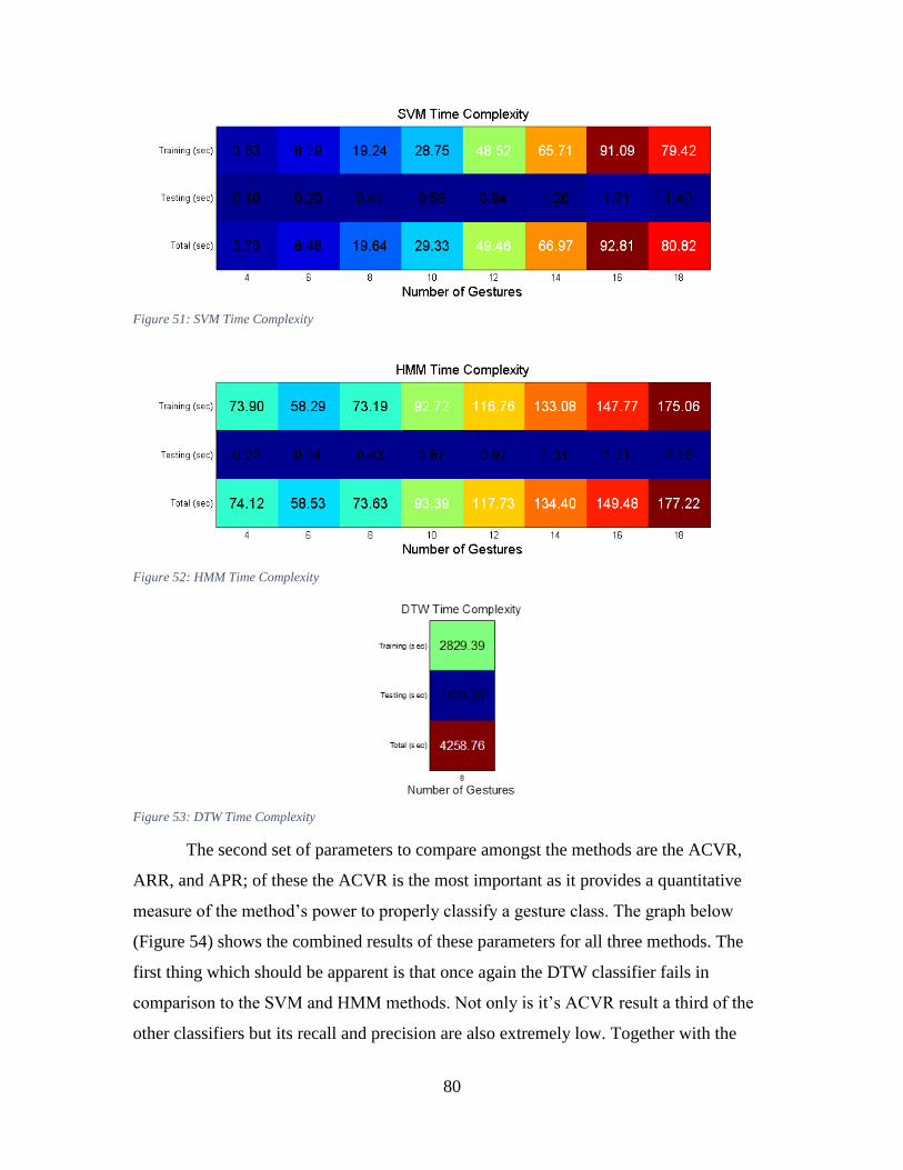
80
Figure 51: SVM Time Complexity
Figure 52: HMM Time Complexity
Figure 53: DTW Time Complexity
The second set of parameters to compare amongst the methods are the ACVR,
ARR, and APR; of these the ACVR is the most important as it provides a quantitative
measure of the method’s power to properly classify a gesture class. The graph below
(Figure 54) shows the combined results of these parameters for all three methods. The
first thing which should be apparent is that once again the DTW classifier fails in
comparison to the SVM and HMM methods. Not only is it’s ACVR result a third of the
other classifiers but its recall and precision are also extremely low. Together with the
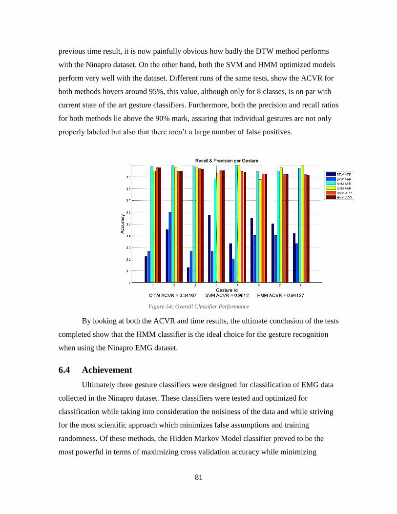
81
previous time result, it is now painfully obvious how badly the DTW method performs
with the Ninapro dataset. On the other hand, both the SVM and HMM optimized models
perform very well with the dataset. Different runs of the same tests, show the ACVR for
both methods hovers around 95%, this value, although only for 8 classes, is on par with
current state of the art gesture classifiers. Furthermore, both the precision and recall ratios
for both methods lie above the 90% mark, assuring that individual gestures are not only
properly labeled but also that there aren’t a large number of false positives.
Figure 54: Overall Classifier Performance
By looking at both the ACVR and time results, the ultimate conclusion of the tests
completed show that the HMM classifier is the ideal choice for the gesture recognition
when using the Ninapro EMG dataset.
6.4 Achievement
Ultimately three gesture classifiers were designed for classification of EMG data
collected in the Ninapro dataset. These classifiers were tested and optimized for
classification while taking into consideration the noisiness of the data and while striving
for the most scientific approach which minimizes false assumptions and training
randomness. Of these methods, the Hidden Markov Model classifier proved to be the
most powerful in terms of maximizing cross validation accuracy while minimizing
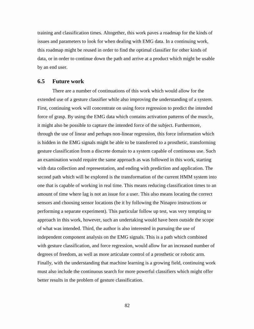
82
training and classification times. Altogether, this work paves a roadmap for the kinds of
issues and parameters to look for when dealing with EMG data. In a continuing work,
this roadmap might be reused in order to find the optimal classifier for other kinds of
data, or in order to continue down the path and arrive at a product which might be usable
by an end user.
6.5 Future work
There are a number of continuations of this work which would allow for the
extended use of a gesture classifier while also improving the understanding of a system.
First, continuing work will concentrate on using force regression to predict the intended
force of grasp. By using the EMG data which contains activation patterns of the muscle,
it might also be possible to capture the intended force of the subject. Furthermore,
through the use of linear and perhaps non-linear regression, this force information which
is hidden in the EMG signals might be able to be transferred to a prosthetic, transforming
gesture classification from a discrete domain to a system capable of continuous use. Such
an examination would require the same approach as was followed in this work, starting
with data collection and representation, and ending with prediction and application. The
second path which will be explored is the transformation of the current HMM system into
one that is capable of working in real time. This means reducing classification times to an
amount of time where lag is not an issue for a user. This also means locating the correct
sensors and choosing sensor locations (be it by following the Ninapro instructions or
performing a separate experiment). This particular follow up test, was very tempting to
approach in this work, however, such an undertaking would have been outside the scope
of what was intended. Third, the author is also interested in pursuing the use of
independent component analysis on the EMG signals. This is a path which combined
with gesture classification, and force regression, would allow for an increased number of
degrees of freedom, as well as more articulate control of a prosthetic or robotic arm.
Finally, with the understanding that machine learning is a growing field, continuing work
must also include the continuous search for more powerful classifiers which might offer
better results in the problem of gesture classification.

83
6.6 Summary
The final chapter of this thesis serves as a conclusion of the work undertaken.
Structuring these concluding remarks has been done by first presenting previous
classification results using the Ninapro dataset, and comparing these results to each of the
three learning methods. Each of these methods were then compared amongst themselves
for accuracy as well as implementation and computational complexity. Ultimately, the
overall achievements were also covered as well as future work which would supplement
and expand this system.
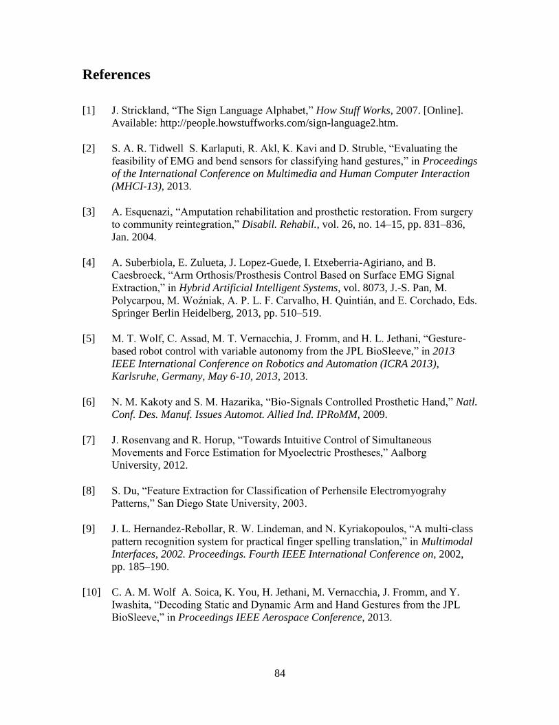
84
References
[1] J. Strickland, “The Sign Language Alphabet,” How Stuff Works, 2007. [Online].
Available: http://people.howstuffworks.com/sign-language2.htm.
[2] S. A. R. Tidwell S. Karlaputi, R. Akl, K. Kavi and D. Struble, “Evaluating the
feasibility of EMG and bend sensors for classifying hand gestures,” in Proceedings
of the International Conference on Multimedia and Human Computer Interaction
(MHCI-13), 2013.
[3] A. Esquenazi, “Amputation rehabilitation and prosthetic restoration. From surgery
to community reintegration,” Disabil. Rehabil., vol. 26, no. 14–15, pp. 831–836,
Jan. 2004.
[4] A. Suberbiola, E. Zulueta, J. Lopez-Guede, I. Etxeberria-Agiriano, and B.
Caesbroeck, “Arm Orthosis/Prosthesis Control Based on Surface EMG Signal
Extraction,” in Hybrid Artificial Intelligent Systems, vol. 8073, J.-S. Pan, M.
Polycarpou, M. Woźniak, A. P. L. F. Carvalho, H. Quintián, and E. Corchado, Eds.
Springer Berlin Heidelberg, 2013, pp. 510–519.
[5] M. T. Wolf, C. Assad, M. T. Vernacchia, J. Fromm, and H. L. Jethani, “Gesture-
based robot control with variable autonomy from the JPL BioSleeve,” in 2013
IEEE International Conference on Robotics and Automation (ICRA 2013),
Karlsruhe, Germany, May 6-10, 2013, 2013.
[6] N. M. Kakoty and S. M. Hazarika, “Bio-Signals Controlled Prosthetic Hand,” Natl.
Conf. Des. Manuf. Issues Automot. Allied Ind. IPRoMM, 2009.
[7] J. Rosenvang and R. Horup, “Towards Intuitive Control of Simultaneous
Movements and Force Estimation for Myoelectric Prostheses,” Aalborg
University, 2012.
[8] S. Du, “Feature Extraction for Classification of Perhensile Electromyograhy
Patterns,” San Diego State University, 2003.
[9] J. L. Hernandez-Rebollar, R. W. Lindeman, and N. Kyriakopoulos, “A multi-class
pattern recognition system for practical finger spelling translation,” in Multimodal
Interfaces, 2002. Proceedings. Fourth IEEE International Conference on, 2002,
pp. 185–190.
[10] C. A. M. Wolf A. Soica, K. You, H. Jethani, M. Vernacchia, J. Fromm, and Y.
Iwashita, “Decoding Static and Dynamic Arm and Hand Gestures from the JPL
BioSleeve,” in Proceedings IEEE Aerospace Conference, 2013.
85
[11] M. Atzori, A. Gijsberts, S. Heynen, A. M. Hager, O. Deriaz, P. van der Smagt, C.
Castellini, B. Caputo, and H. Muller, “Building the Ninapro database: A resource
for the biorobotics community,” in Biomedical Robotics and Biomechatronics
(BioRob), 2012 4th IEEE RAS & EMBS International Conference on, 2012, pp.
1258–1265.
[12] A. Gijsberts, M. Atzori, C. Castellini, H. Muller, and B. Caputo, “The Movement
Error Rate for Evaluation of Machine Learning Methods for sEMG-based Hand
Movement Classification,” Neural Syst. Rehabil. Eng. IEEE Trans., vol. PP, no.
99, p. 1, 2014.
[13] “ThalmicLabs.” [Online]. Available: https://www.thalmic.com/en/myo/.
[Accessed: 04-Aug-2014].
[14] P. Zhou, M. M. Lowery, K. B. Englehart, H. Huang, G. Li, L. Hargrove, J. P. a
Dewald, and T. a Kuiken, “Decoding a new neural machine interface for control of
artificial limbs.,” J. Neurophysiol., vol. 98, no. 5, pp. 2974–82, Nov. 2007.
[15] G. Li, “Electromyography Pattern-Recognition-Based Control of Powered
Multifunctional Upper-Limb Prostheses,” in Advances in Applied
Electromyography, J. Mizrahi, Ed. 2011.
[16] T. Pylv and T. Pylvänäinen, “Accelerometer Based Gesture Recognition Using
Continuous HMMs,” in Pattern Recognition and Image Analysis, vol. 3522, J.
Marques, N. Pérez de la Blanca, and P. Pina, Eds. Springer Berlin Heidelberg,
2005, pp. 639–646.
[17] N. E. Gillian, “Gesture Recognition for Musician Computer Interaction,” Queen’s
University Belfast, Ireland, 2011.
[18] M. Wöllmer, M. Al-Hames, F. Eyben, B. Schuller, and G. Rigoll, “A
multidimensional dynamic time warping algorithm for efficient multimodal fusion
of asynchronous data streams,” Neurocomputing, vol. 73, no. 1–3, pp. 366–380,
2009.
[19] I. Koprinska, “Feature selection for brain-computer interfaces,” New Front. Appl.
Data Min., 2010.
[20] D. Tkach, H. Huang, and T. a Kuiken, “Study of stability of time-domain features
for electromyographic pattern recognition.,” J. Neuroeng. Rehabil., vol. 7, p. 21,
Jan. 2010.
[21] C. Xiang, Z. Xu, Z. Zhang-Yan, Y. Ji-Hai, V. Lantz, W. Kong-Qiao, X. Chen, X.
Zhang, Z.-Y. Zhao, J.-H. Yang, and K.-Q. Wang, “Hand Gesture Recognition
Research Based on Surface EMG Sensors and 2D-accelerometers,” in Wearable
Computers, 2007 11th IEEE International Symposium on, 2007, pp. 11–14.

86
[22] N. S. Rekhi, A. S. Arora, S. Singh, and D. Singh, “Multi-Class SVM Classification
of Surface EMG Signal for Upper Limb Function,” in Bioinformatics and
Biomedical Engineering , 2009. ICBBE 2009. 3rd International Conference on,
2009, pp. 1–4.
[23] M. V Liarokapis, P. K. Artemiadis, P. T. Katsiaris, and K. J. Kyriakopoulos,
“Learning task-specific models for reach to grasp movements: Towards EMG-
based teleoperation of robotic arm-hand systems,” in Biomedical Robotics and
Biomechatronics (BioRob), 2012 4th IEEE RAS & EMBS International Conference
on, 2012, pp. 1287–1292.
[24] Z. Xu, C. Xiang, L. Yun, V. Lantz, W. Kongqiao, Y. Jihai, X. Zhang, X. Chen, A.
Member, Y. Li, K. Wang, and J. Yang, “A Framework for Hand Gesture
Recognition Based on Accelerometer and EMG Sensors,” Syst. Man Cybern. Part
A Syst. Humans, IEEE Trans., vol. 41, no. 6, pp. 1064–1076, 2011.
[25] G. A. Garcia, R. Okuno, and K. Azakawa, “A decomposition algorithm for surface
electrode-array electromyogram,” Eng. Med. Biol. Mag. IEEE, vol. 24, no. 4, pp.
63–72, 2005.
[26] N. Shapiro, “Motor Unit Recruitment Strategies During Deep Muscle Pain,” The
alchemist. [Online]. Available: http://natchem.wordpress.com/2009/11/23/motor-
unit-recruitment-strategies-during-deep-muscle-pain/.
[27] A. Zeghbib, Forearm Surface EMG Signals Recognition and Muscoloskeletal
System Dynamics Identification Using Intelligent Computational Methods. 2007,
p. 229.
[28] J. Kim, S. Mastnik, E. Andr, and #233, “EMG-based hand gesture recognition for
realtime biosignal interfacing,” Proceedings of the 13th international conference
on Intelligent user interfaces. ACM, Gran Canaria, Spain, pp. 30–39, 2008.
[29] G. R. Naik, D. K. Kumar, V. P. Singh, and M. Palaniswami, “Hand gestures for
HCI using ICA of EMG,” Proceedings of the HCSNet workshop on Use of vision
in human-computer interaction - Volume 56. Australian Computer Society, Inc.,
Canberra, Australia, pp. 67–72, 2006.
[30] A. S. Mannini Angelo Maria, A. Mannini, and A. M. Sabatini, “Machine Learning
Methods for Classifying Human Physical Activity from On-Body
Accelerometers,” Sensors, vol. 10, no. 2, pp. 1154–1175, Jan. 2010.
[31] M. Müller, “Dynamic Time Warping,” in Information Retrieval for Music and
Motion, Springer Berlin Heidelberg, 2007, pp. 69–84.
87
[32] C. R. Souza, “Kernel Functions for Machine Learning Applications,” 2010.
[Online]. Available: http://crsouza.blogspot.com/2010/03/kernel-functions-for-
machine-learning.html. [Accessed: 08-Jan-2014].
[33] R. N. Khushaba, S. Kodagoda, M. Takruri, and G. Dissanayake, “Toward
improved control of prosthetic fingers using surface electromyogram (EMG)
signals,” Expert Syst. Appl., vol. 39, no. 12, pp. 10731–10738, 2012.
[34] B. Direito, J. Duarte, and C. Teixeira, “Feature selection in high dimensional EEG
features spaces for epileptic seizure prediction,” Proc. 18th IFAC …, 2011.
[35] R. Chowdhury, M. Reaz, M. Ali, A. Bakar, K. Chellappan, and T. Chang, “Surface
Electromyography Signal Processing and Classification Techniques,” Sensors, vol.
13, no. 9, pp. 12431–12466, 2013.
[36] A. Phinyomark, “A novel feature extraction for robust EMG pattern recognition,”
arXiv Prepr. arXiv …, vol. 1, no. 1, pp. 71–80, 2009.
[37] A. Hussein Ali, “An Investigation of Electromyographic (EMG) Control of
Dextrous Hand Prostheses for Transradian Amputees,” Ieee, 2013.
[38] A. D. C. Chan and G. C. Green, “Myoelectric control development toolbox,” Proc.
30th Conf. Can. Med. Biol. Eng. Soc., vol. 1, pp. M0100–1, 2007.
[39] A. Shakoor, T. May, and N. Van Schijndel, “Soft computing based feature
selection for environmental sound classification,” Blekinge Institute of
Technology, 2010.
[40] S. Chakrabarti, B. Dom, R. Agrawal, and P. Raghavan, “Scalable feature selection,
classification and signature generation for organizing large text databases into
hierarchical topic taxonomies,” VLDB J. Int. J. Very Large Data Bases, vol. 7, no.
3, pp. 163–178, Aug. 1998.
[41] S.-Y. Kung and M.-W. Mak, “Feature Selection for Genomic and Proteomic Data
Mining,” in Machine Learning in Bioinformatics, Y. Pan and A. Y. Zomaya, Eds.
JOHN WILEY & SONS, INC., 2009, pp. 1–46.
[42] I. Guyon, “An Introduction to Variable and Feature Selection,” J. Mach. Learn.
Res., vol. 3, pp. 1157–1182, 2003.
[43] J. B. MacQueen, “Some Methods for classification and Analysis of Multivariate
Observations,” in Proceedings of 5-th Berkeley Symposium on Mathematical
Statistics and Probability, 1967, pp. 281–297.
[44] T. T. Swee, A. K. Ariff, S. H. Salleh, S. Siew Kean, and H. Leong Seng, “Wireless
data gloves Malay sign language recognition system,” in Information,
88
Communications & Signal Processing, 2007 6th International Conference on,
2007, pp. 1–4.
[45] X. Chen and Z. J. Wang, “Pattern recognition of number gestures based on a
wireless surface EMG system,” Biomed. Signal Process. Control, vol. 8, no. 2, pp.
184–192, Mar. 2013.
[46] C. Chang and C. Lin, “LIBSVM: a library for support vector machines,” ACM
Trans. Intell. Syst. …, vol. 2, no. 3, pp. 1–39, 2011.
[47] C.-J. Lin, “Errata to ‘A comparison of methods for multiclass support vector
machines’.,” IEEE Trans. Neural Netw., vol. 13, no. 4, pp. 1026–7, Jan. 2002.
[48] C. Hsu, C. Chang, and C. Lin, “A Practical Guide to Support Vector
Classification,” vol. 1, no. 1, pp. 1–16, 2010.
[49] M. Atzori, “Characterization of a Benchmark Database for Myoelectric Movement
Classification,” Neural Syst. Rehabil. Eng., vol. PP, no. 99, 2014.
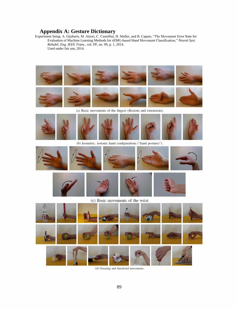
89
Appendix A: Gesture Dictionary Experiment Setup, A. Gijsberts, M. Atzori, C. Castellini, H. Muller, and B. Caputo, “The Movement Error Rate for
Evaluation of Machine Learning Methods for sEMG-based Hand Movement Classification,” Neural Syst.
Rehabil. Eng. IEEE Trans., vol. PP, no. 99, p. 1, 2014.
Used under fair use, 2014.
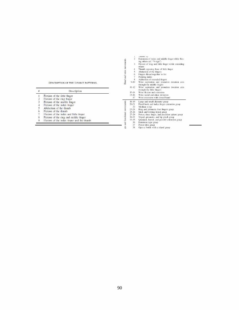
90
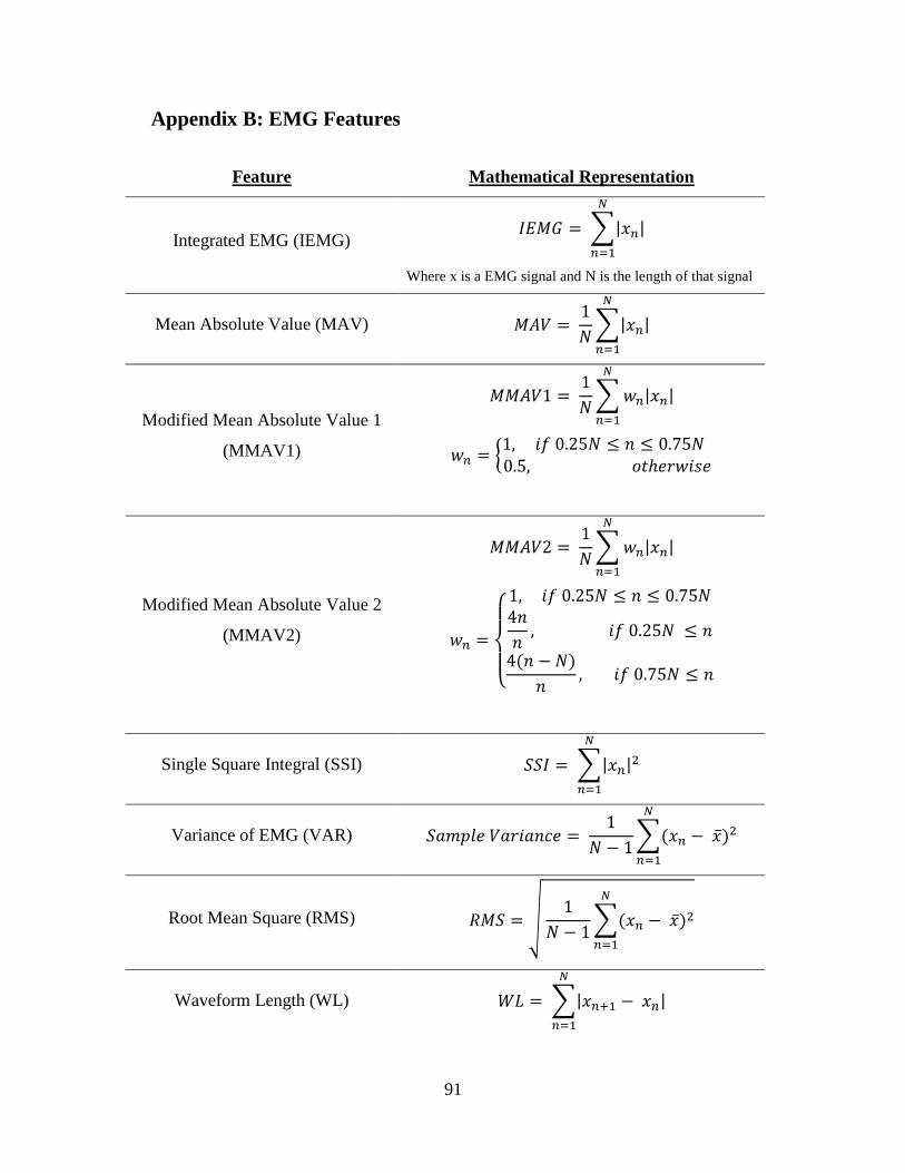
91
Appendix B: EMG Features
Feature Mathematical Representation
Integrated EMG (IEMG) ∑
Where x is a EMG signal and N is the length of that signal
Mean Absolute Value (MAV)
∑
Modified Mean Absolute Value 1
(MMAV1)
∑
{
Modified Mean Absolute Value 2
(MMAV2)
∑
{
Single Square Integral (SSI) ∑
Variance of EMG (VAR)
∑
Root Mean Square (RMS) √
∑
Waveform Length (WL) ∑
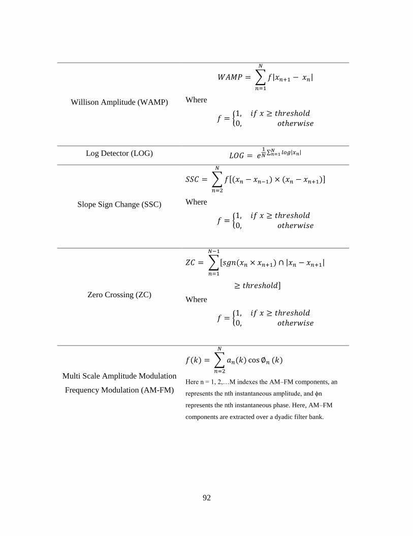
92
Willison Amplitude (WAMP)
∑
Where
{
Log Detector (LOG)
∑
Slope Sign Change (SSC)
∑
Where
{
Zero Crossing (ZC)
∑
Where
{
Multi Scale Amplitude Modulation
Frequency Modulation (AM-FM)
∑
Here n = 1, 2,…M indexes the AM–FM components, an
represents the nth instantaneous amplitude, and ϕn
represents the nth instantaneous phase. Here, AM–FM
components are extracted over a dyadic filter bank.