machine learning techniques for word sense disambiguationescudero/wsd/06-tesi.pdf · machine...
TRANSCRIPT

Thesis Dissertation:
Machine Learning Techniques
for
Word Sense Disambiguation
Gerard Escudero Bakx
Thesis advisors:
Lluıs Marquez Villodre and German Rigau Claramunt
For the obtention of the PhD Degree at the
Universitat Politecnica de Catalunya
Barcelona, May 22, 2006


Abstract
In the Natural Language Processing (NLP) community, Word Sense Disambiguation(WSD) has been described as the task which selects the appropriate meaning (sense)to a given word in a text or discourse where this meaning is distinguishable from othersenses potentially attributable to that word. These senses could be seen as the targetlabels of a classification problem. That is, Machine Learning (ML) seems to be a possibleway to tackle this problem.
This work studies the possible application of the algorithms and techniques of theMachine Learning field in order to handle the WSD task.
The first issue treated has been the adaptation of alternative ML algorithms to dealwith word senses as classes. Then, a comparison of these methods is performed under thesame conditions. The evaluation measures applied to compare the performances of thesemethods are the typical precision and recall, but also agreement rates and kappa statistics.
The second topic explored is the cross-corpora application of supervised MachineLearning systems for WSD to test the generalisation ability across corpora and domains.The results obtained are very disappointing, seriously questioning the possibility ofconstructing a general enough training corpus (labelled or unlabelled), and the way itsexamples should be used to develop a general purpose Word Sense Tagger.
The use of unlabelled data to train classifiers for Word Sense Disambiguation is a verychallenging line of research in order to develop a really robust, complete and accurateWord Sense Tagger. Due to this fact, the next topic treated in this work is the applicationof two bootstrapping approaches on WSD: the Transductive Support Vector Machines andthe Greedy Agreement bootstrapping algorithm by Steven Abney.
During the development of this research we have been interested in the construction andevaluation of several WSD systems. We have participated in the last two editions of theEnglish Lexical Sample task of Senseval evaluation exercises. The Lexical Sample tasks aremainly oriented to evaluate Supervised Machine Learning systems. Our systems achieved
i

a very good performance in both editions of this competition. That is, our systems areamong the state-of-the-art on WSD. As a complementary work of this participation, someother issues have been explored: 1) a comparative study of the features used to representexamples for WSD; 2) the comparison of different feature selection procedures; and 3) anstudy of the results of the best systems of Senseval-2 that shows the real behaviour ofthese systems with respect to the data.
Summarising, this work has: 1) studied the application of Machine Learning to WordSense Disambiguation; and 2) described our participation on the English Lexical Sampletask of both Senseval-2 and Senseval-3 international evaluation exercises. This work hasclarified several open questions which we think will help to understand this complexproblem.
ii

Acknowledgements
We want to specially thank to Victoria Arranz for her help with English writing; to DavidMartınez for their useful comments and discussions; to Adria Gispert for its perl scripts;to Yarowsky’s group for the feature extractor of syntactical patterns; to the referees ofinternational conferences and of the previous version of this document for their helpfulcomments; to Victoria Arranz, Jordi Atserias, Laura Benıtez and Montse Civit for theirfriendship; and to Montse Beseran for its infinity patience and love.
We want to also thank to Lluıs Marquez and German Rigau for all these years ofdedication; to Horacio Rodrıguez for his humanity; to Eneko Agirre for his comments;and to all the members of the TALP Research Centre of the Software Department of theTechnical University of Catalonia for working together.
This research has been partially funded by the European Commission viaEuroWordNet (LE4003), NAMIC (IST-1999-12392) and MEANING (IST-2001-34460)projects; by the Spanish Research Department via ITEM (TIC96-1243-C03-03),BASURDE (TIC98-0423-C06) and HERMES (TIC2000-0335-C03-02); and by the CatalanResearch Department VIA CIRIT’s consolidated research group 1999SGR-150, CREL’sCatalan WordNet project and CIRIT’s grant 1999FI-00773.
iii

iv
Contents
Abstract i
Acknowledgements iii
1 Introduction 1
1.1 Usefulness of WSD . . . . . . . . . . . . . . . . . . . . . . . . . . . . . . . . 2
1.2 Thesis Contributions . . . . . . . . . . . . . . . . . . . . . . . . . . . . . . . 3
1.3 Thesis Layout . . . . . . . . . . . . . . . . . . . . . . . . . . . . . . . . . . . 4
2 State-of-the-Art 7
2.1 The Word Sense Disambiguation Task . . . . . . . . . . . . . . . . . . . . . 8
2.1.1 Knowledge-based Methods . . . . . . . . . . . . . . . . . . . . . . . . 9
2.1.2 Corpus-based Approach . . . . . . . . . . . . . . . . . . . . . . . . . 12
2.1.3 Corpus for training Supervised Methods . . . . . . . . . . . . . . . . 12
2.1.4 Porting across corpora . . . . . . . . . . . . . . . . . . . . . . . . . . 15
2.1.5 Feature selection and parameter optimisation . . . . . . . . . . . . . 16
2.2 Supervised Corpus-based Word Sense Disambiguation . . . . . . . . . . . . 18
2.2.1 Word Sense Disambiguation Data . . . . . . . . . . . . . . . . . . . 18
2.2.2 Representation of Examples . . . . . . . . . . . . . . . . . . . . . . . 21
2.2.3 Main Approaches to Supervised WSD . . . . . . . . . . . . . . . . . 22
2.3 Current Open Issues . . . . . . . . . . . . . . . . . . . . . . . . . . . . . . . 28
v

CONTENTS
2.3.1 Bootstrapping Approaches . . . . . . . . . . . . . . . . . . . . . . . . 28
2.4 Evaluation . . . . . . . . . . . . . . . . . . . . . . . . . . . . . . . . . . . . . 30
2.4.1 Pre-Senseval evaluations . . . . . . . . . . . . . . . . . . . . . . . . . 30
2.4.2 Senseval Evaluation . . . . . . . . . . . . . . . . . . . . . . . . . . . 32
2.5 Further Readings . . . . . . . . . . . . . . . . . . . . . . . . . . . . . . . . . 38
3 A Comparison of Supervised ML Algorithms for WSD 39
3.1 Machine Learning for Classification . . . . . . . . . . . . . . . . . . . . . . . 40
3.1.1 Naive Bayes . . . . . . . . . . . . . . . . . . . . . . . . . . . . . . . . 41
3.1.2 Exemplar-based learning . . . . . . . . . . . . . . . . . . . . . . . . . 42
3.1.3 Decision Lists . . . . . . . . . . . . . . . . . . . . . . . . . . . . . . . 44
3.1.4 AdaBoost . . . . . . . . . . . . . . . . . . . . . . . . . . . . . . . . . 44
3.1.5 Support Vector Machines . . . . . . . . . . . . . . . . . . . . . . . . 48
3.2 Setting . . . . . . . . . . . . . . . . . . . . . . . . . . . . . . . . . . . . . . . 51
3.2.1 Corpora . . . . . . . . . . . . . . . . . . . . . . . . . . . . . . . . . . 51
3.2.2 Basic Features . . . . . . . . . . . . . . . . . . . . . . . . . . . . . . 51
3.3 Adapting Naive-Bayes and Exemplar-Based Algorithms . . . . . . . . . . . 53
3.3.1 Comments about Related Work . . . . . . . . . . . . . . . . . . . . . 53
3.3.2 Description of the Experiments . . . . . . . . . . . . . . . . . . . . . 54
3.3.3 Conclusions . . . . . . . . . . . . . . . . . . . . . . . . . . . . . . . . 59
3.4 Applying the AdaBoost Algorithm . . . . . . . . . . . . . . . . . . . . . . . 59
3.4.1 Description of the Experiments . . . . . . . . . . . . . . . . . . . . . 60
3.4.2 Conclusions . . . . . . . . . . . . . . . . . . . . . . . . . . . . . . . . 65
3.5 Comparison of Machine Learning Methods . . . . . . . . . . . . . . . . . . . 65
3.5.1 Setting of Evaluation . . . . . . . . . . . . . . . . . . . . . . . . . . . 66
3.5.2 Discussion . . . . . . . . . . . . . . . . . . . . . . . . . . . . . . . . . 67
3.6 Conclusions . . . . . . . . . . . . . . . . . . . . . . . . . . . . . . . . . . . . 70
vi

CONTENTS
4 Domain Dependence 73
4.1 Introduction . . . . . . . . . . . . . . . . . . . . . . . . . . . . . . . . . . . . 73
4.2 Setting . . . . . . . . . . . . . . . . . . . . . . . . . . . . . . . . . . . . . . . 74
4.3 First Experiment: Across Corpora evaluation . . . . . . . . . . . . . . . . . 75
4.4 Second Experiment: tuning to new domains . . . . . . . . . . . . . . . . . . 77
4.5 Third Experiment: training data quality . . . . . . . . . . . . . . . . . . . . 77
4.6 Conclusions . . . . . . . . . . . . . . . . . . . . . . . . . . . . . . . . . . . . 81
5 Bootstrapping 83
5.1 Transductive SVMs . . . . . . . . . . . . . . . . . . . . . . . . . . . . . . . . 83
5.1.1 Setting . . . . . . . . . . . . . . . . . . . . . . . . . . . . . . . . . . 84
5.1.2 Experiments with TSVM . . . . . . . . . . . . . . . . . . . . . . . . 86
5.2 Greedy Agreement Bootstrapping Algorithm . . . . . . . . . . . . . . . . . 91
5.2.1 Setting . . . . . . . . . . . . . . . . . . . . . . . . . . . . . . . . . . 92
5.2.2 Experimental Evaluation . . . . . . . . . . . . . . . . . . . . . . . . 94
5.3 Conclusions and Current/Further Work . . . . . . . . . . . . . . . . . . . . 101
6 Evaluation in Senseval Exercises 103
6.1 Senseval Corpora . . . . . . . . . . . . . . . . . . . . . . . . . . . . . . . . . 103
6.2 TALP System at Senseval-2 . . . . . . . . . . . . . . . . . . . . . . . . . . . 104
6.2.1 Feature Set . . . . . . . . . . . . . . . . . . . . . . . . . . . . . . . . 105
6.2.2 Preprocessing and Hierarchical Decomposition . . . . . . . . . . . . 108
6.2.3 Evaluation . . . . . . . . . . . . . . . . . . . . . . . . . . . . . . . . 109
6.3 From Senseval-2 to Senseval-3 . . . . . . . . . . . . . . . . . . . . . . . . . . 111
6.3.1 System Decomposition . . . . . . . . . . . . . . . . . . . . . . . . . . 112
6.3.2 The TalpSVM System . . . . . . . . . . . . . . . . . . . . . . . . . . 116
6.3.3 Global Results . . . . . . . . . . . . . . . . . . . . . . . . . . . . . . 121
6.4 Senseval-3 . . . . . . . . . . . . . . . . . . . . . . . . . . . . . . . . . . . . . 121
vii
CONTENTS
6.4.1 Learning Framework . . . . . . . . . . . . . . . . . . . . . . . . . . . 123
6.4.2 Features . . . . . . . . . . . . . . . . . . . . . . . . . . . . . . . . . . 124
6.4.3 Experimental Setting . . . . . . . . . . . . . . . . . . . . . . . . . . . 124
6.4.4 Evaluation . . . . . . . . . . . . . . . . . . . . . . . . . . . . . . . . 126
6.4.5 Extending the Feature Selection process . . . . . . . . . . . . . . . . 127
6.5 Conclusions . . . . . . . . . . . . . . . . . . . . . . . . . . . . . . . . . . . . 129
7 Conclusions 131
7.1 Summary . . . . . . . . . . . . . . . . . . . . . . . . . . . . . . . . . . . . . 131
7.2 Contributions . . . . . . . . . . . . . . . . . . . . . . . . . . . . . . . . . . . 133
7.3 Publications . . . . . . . . . . . . . . . . . . . . . . . . . . . . . . . . . . . . 134
7.4 Further Work . . . . . . . . . . . . . . . . . . . . . . . . . . . . . . . . . . . 135
Bibliography 137
A Statistical Measures 153
A.1 Evaluation Measures . . . . . . . . . . . . . . . . . . . . . . . . . . . . . . . 153
A.2 Significance Tests . . . . . . . . . . . . . . . . . . . . . . . . . . . . . . . . . 154
A.3 Agreement and Kappa statistic . . . . . . . . . . . . . . . . . . . . . . . . . 154
B Example of the Feature Extractor 155
C Resources and Web References 159
D List of Acronyms 161
viii
Chapter 1
Introduction
Since the appearance of the first computers, in the earlier 50’s, humans have been thinkingin Natural Language Understanding (NLU). Since then, lots of talking computers appearedin fiction novels and films. Humans usually see computers as intelligent devices. However,the pioneers of Natural Language Processing (NLP) underestimated the complexity of thetask. Unfortunately, natural language systems seems to require extensive knowledge aboutthe world which in turn it is not easy to acquire. NLP community has been researchingon NLU for 50 years and satisfactory results have been obtained only for very restricteddomains1.
It is commonly assumed that NLU is related with semantics. NLP community haveapplied different ways to tackle semantics, such as logical formalisms or frames to representthe necessary knowledge. The current usual way to tackle NLP is as a process chain, inwhich each step of the chain is devoted to one Natural Language task; usually tryingto solve a particular Natural Language ambiguity problem. Natural language presentsmany types of ambiguity, ranging from morphological ambiguity to pragmatic ambiguitypassing through syntactic or semantic ambiguities. Thus, most efforts in Natural LanguageProcessing are devoted to solve different types of ambiguities, such as: part-of-speech(POS) tagging –dealing with morphosyntactic categories– or parsing –dealing with syntax.
The work presented here focus on lexical or word sense ambiguity. That is, theambiguity related to the polisemy of words (isolated words are ambiguous). Thedetermination of the meaning of each word of a context seems to be a necessity in orderto understand the language. Lexical ambiguity is a long-standing problem in NLP, whichappears on early references (Kaplan, 1950; Yngve, 1955) on Machine Translation2.
1See Winograd SHRDLU program (Winograd, 1972).2Wikipedia points Word Sense Disambiguation as one of the big difficulties for NLP.
1

1 Introduction
Lexical Ambiguity Resolution or Word Sense Disambiguation (WSD) is the problemof assigning the appropriate meaning (sense) to a given word in a text or discourse wherethis meaning is distinguishable from other senses potentially attributable to that word(Ide and Veronis, 1998). Thus, a WSD or Word Sense Tagging system must be able toassign the correct sense of a given word, for instance age, depending on the context inwhich the word occurs.
Table 1.1 shows, as an example, two of the senses of noun age, their translation intoCatalan and two glosses describing their meaning3. Sense 1 of word age is translatedinto Catalan as edat and sense 2 to the noun era, which indicates a real word sensedistinction. An NLP system trying to capture the intended meaning of the word age inthe two sentences in table 1.2 would performing word sense disambiguation4.
English Catalan glossage 1 edat the length of time something (or someone)
has existedage 2 era a historic period
Table 1.1: Definitions of two of the senses of word age from WordNet 1.5.
sense glossage 1 He was mad about stars at the age of nine .age 2 About 20,000 years ago the last ice age ended .
Table 1.2: Examples from DSO corpus.
1.1 Usefulness of WSD
WSD task is a potential intermediate task (Wilks and Stevenson, 1996) for manyother NLP systems, including mono and multilingual Information Retrieval, InformationExtraction, Machine Translation or Natural Language Understanding.
Resolving the sense ambiguity of words is obviously essential for many NaturalLanguage Understanding applications (Ide and Veronis, 1998). However, current NLUapplications are mostly domain specific (Kilgarriff, 1997; Viegas et al., 1999). Obviously,when restricting the application to a domain we are, in fact, using the “one sense perdiscourse” hypothesis to eliminate most of the semantic ambiguity of polysemous words(Gale et al., 1992b).
3The English information of this table has been extracted from WordNet 1.5 (Miller et al., 1990).4These sentences have been extracted from the DSO corpus (Ng and Lee, 1996).
2

1.2 Thesis Contributions
Furthermore, the need of enhanced WSD capabilities appears in many applicationswhose aim is not language understanding. Among others, we could mention:
• Machine Translation: This is the field in which the first attempts to perform WSDwhere carried out (Weaver, 1955; Yngve, 1955; Bar-Hillel, 1960). There is no doubtthat some kind of WSD is essential for the proper translation of polysemous words.
• Information Retrieval : in order to discard occurrences of words in documentsappearing with inappropriate senses (Salton, 1968; Salton and McGill, 1983; Krovetzand Croft, 1992; Voorhees, 1993; Schutze and Pedersen, 1995).
• Semantic Parsing : Alshawi and Carter (1994) suggest the utility of WSD inrestricting the space of competing parses, especially, for the dependencies, such asprepositional phrases.
• Speech Synthesis and Recognition: WSD could be useful for the correct phonetisationof words in Speech Synthesis (Sproat et al., 1992; Yarowsky, 1997), and for wordsegmentation and homophone discrimination in Speech Recognition (Connine, 1990;Seneff, 1992).
• Acquisition of Lexical Knowledge: many approaches designed to automaticallyacquire large-scale NLP resources such as, selectional restrictions (Ribas, 1995),subcategorisation verbal patterns (Briscoe and Carroll, 1997), translation links(Atserias et al., 1997) have obtained limited success because of the use of limitedWSD approaches.
• Lexicography : Kilgarriff (1997) suggests that lexicographers can be not only suppliersof NLP resources, but also customers of WSD systems.
Unfortunately, the low accuracy results obtained by current state-of-the-art WSDsystems seem to be below practical requirements. Carpuat and Wu (2005) studied theusefulness of WSD to Statistical Machine Translation and, with a few exceptions, noimprovement was achieved in their experiments. They also questioned the current modelsof Statistical MT.
1.2 Thesis Contributions
The main contribution of this thesis is to explore the possible application of algorithmsand techniques of the Machine Learning field to the Word Sense Disambiguation. We havesummarised below the list of contributions we consider most important from this work:
3
1 Introduction
Comparative study: First, we have performed a comparison of the most usedalgorithms in the research literature. During this process, we have clarified some confusinginformation on the literature and developed some improvements on the adaptation ofsome algorithms (in terms of representation of the information and efficiency). We haveempirically demonstrated that the best systems on Word Sense Disambiguation data arethose based on margin-maximisation. We have also seen that accuracy, agreement, andKappa statistics show interesting dimensions when evaluating the systems.
Generalisation across corpora: The experiments of chapter 4 empirically show thedependency of Machine Learning on the training corpora. This issue has to be solved inorder to develop a real and useful Word Sense Tagger. Until knowing the way of buildingfull general corpora or flexible training procedures able to adapt to changing objectivefunctions, the only Word Sense Taggers we can build are those based on restricted domains.
Bootstrapping: The experiments of chapter 5 explore two Bootstrapping techniques:Transductive Support Vector Machines and the greedy agreement Abney’s algorithm. Thefirst approach does not proved to work properly. However, the Abney’s algorithm showedbetter performance. Initial experiments seem to indicate a promising line of research.
International Evaluation Exercises on WSD: We also have participated on theEnglish Lexical Sample task of both Senseval-2 and Senseval-3 competitions with twodifferent systems obtaining very good results. On Senseval-2 our system got the fifthposition at only 4.8% of accuracy from the winner, and on Senseval-3 our system achievedthe seventh position at only 1.6% of accuracy. In both cases, our system proved tobe competitive with state of the art WSD systems. A complementary work has beendeveloped: an study of the sources of the differences among the top performing systemsat Senseval-2.
1.3 Thesis Layout
This section is devoted to overview the contents of the rest of the thesis:
• A survey of the State of the Art on WSD is presented in chapter 2.
• Chapter 3 contains a comparison of the most used Machine Learning algorithmson the Word Sense Disambiguation community. It also reviews other previous
4

1.3 Thesis Layout
comparison works, and explains how the algorithms should be adapted to deal withthe word senses.
• In chapter 4 the cross-corpora application of Machine Learning techniques on WordSense Disambiguation is empirically studied.
• Chapter 5 analyses the usefulness of two bootstrapping techniques on Word SenseDisambiguation.
• Chapter 6 describes our participation in the English Lexical Sample task of bothSenseval-2 and Senseval-3 evaluation exercises. It also shows an study of the bestperforming systems in Senseval-2.
• Finally, the conclusions of our research are presented in chapter 7.
There are four appendixes in this document. The first one shows the formulae ofthe statistical measures applied in all the documents for evaluation purposes. The secondappendix describes in detail (with an example) the output of the feature extractor resultingof this work. The third appendix contains a list of web references of all resources relatedWSD. And the final one contains a list of the acronyms used throughout all the text.
5

1 Introduction
6

Chapter 2
State-of-the-Art
This chapter is devoted to present the state-of-the-art of WSD. Several approaches havebeen proposed for assigning the correct sense to a word in context1, some of them achievingremarkable high accuracy figures. Initially, these methods were usually tested only on asmall set of words with few and clear sense distinctions, e.g. Yarowsky (1995b) reports96% precision for twelve words with only two clear sense distinctions each. Despite thewide range of approaches investigated and the large effort devoted to tackle this problem,it is a fact that to date, no large-scale broad-coverage and highly accurate WSD system hasbeen built. It still remains an open problem if we look at the main conclusions of the ACLSIGLEX Workshop: Tagging Text with Lexical Semantics: Why, What and How? “WSDis perhaps the great open problem at the lexical level of NLP” (Resnik and Yarowsky, 1997)or to the results of the Senseval (Kilgarriff and Rosenzweig, 2000), Senseval-2 (Kilgarriff,2001) and Senseval-3 (Mihalcea et al., 2004) evaluation exercises for WSD; in which noneof the systems presented in these conferences achieved 80% accuracy on both EnglishLexical Sample and All Words tasks. Actually, in the last two competitions the bestsystems achieved accuracy values near 65%.
WSD has been described as an AI-complete problem in the literature, that is, “itssolution requires a solution to all the general Artificial Intelligence (AI) (problems ofrepresenting and reasoning about arbitrary real-world knowledge” (Kilgarriff, 1997) or “aproblem which can be solved only by first resolving all the difficult problems in AI, such asthe representation of common sense and encyclopedic knowledge” (Ide and Veronis, 1998).This fact evinces the hardness of the task and, the large amount of resources needed totackle the problem.
1The most simple approach ignore context and selects for each ambiguous word its most frequent sense
(Gale et al., 1992a; Miller et al., 1994).
7

2 State-of-the-Art
This chapter has been organised as follows: section 2.1 is devoted to describe the task athand and the different ways to address this problem. Then, we focus on the corpus-basedapproach, which is the framework of this thesis. In section 2.2 we extend the corpus-basedexplanation by showing some WSD data, the main corpus-based approaches and the wayWSD data is represented. Section 2.3 is devoted to present a set of promising researchlines in the field, and section 2.4 to several evaluation issues. Finally, section 2.5 containsreferences for extending several issues of the state-of-the-art.
2.1 The Word Sense Disambiguation Task
WSD typically involves two main tasks. On the one hand (1) determining the differentpossible senses (or meanings) of each word, and, on the other hand (2) tagging each wordof a text with its appropriate sense with high accuracy and efficiency.
The former task, that is, the precise definition of a sense, is still under discussionand remains as an open problem within the NLP community. Section 2.2.1 enumeratesthe most important sense repositories used by the Computational Linguistics Community.At the moment, the most used Sense Repository is WordNet. However, many problemsarise mainly related to the granularity of the senses. Contrary to the intuition that theagreement between human annotators should be very high in the WSD task (using aparticular sense repository), some papers report surprisingly low figures. For instance,(Ng et al., 1999) reports an agreement rate of 56.7% and a Kappa value of 0.317 whencomparing the annotation of a subset of the DSO corpus performed by two independentresearch groups2. Similarly, Veronis (1998) reports values of Kappa near to zero whenannotating some special words for the Romanseval corpus3. These reports evince thefragility of existing sense repositories. Humans can not agree in the meaning of a worddue to the subtle and fine distinctions of the sense repositories, lack of clear guidelines,and tight time constraints and limited experience of the human annotators. Moreover,Senseval-3 has shown the dependence of the sense repositories on the accuracy of thesystems. The English Lexical Sample task used as sense repository WordNet and the bestsystem achieved an accuracy of 72.9% (Mihalcea et al., 2004). On the other side, forCatalan and Spanish Lexical Sample tasks, the organisers developed a sense repository
2The Kappa statistic k (Cohen, 1960) (see appendix A) is a good measure for inter-annotator agreement
because reduces the effect of chance agreement. A Kappa value of 1 indicates perfect agreement, while 0.8
is considered as indicating good agreement (Carletta, 1996).3Romanseval is, like Senseval for English, a specific competition between WSD systems for Romance
languages at the moment of first Senseval event. In Senseval-2 and 3 events, Romanseval tasks have become
part of Senseval.
8

2.1 The Word Sense Disambiguation Task
based on coarser grained senses and the best systems achieved respectively 85.8% and84.2% (Marquez et al., 2004b,a). However, the discussion on the most appropriate senserepository for WSD is beyond the scope of the work presented here.
The second task, the tagging of each word with a sense, involves the development ofa system capable of tagging polysemic words in running text with sense labels4. TheWSD community accepts a classification of these systems in two main general categories:knowledge-based and corpus-based methods. All methods build a representation of theexamples to be tagged using some previous information. The difference between themis the source of this information. Knowledge-based methods obtain the informationfrom external knowledge sources such as Machine Readable Dictionaries (MRDs) orlexico-semantic ontologies. This knowledge exists previous to the disambiguation process,and usually have been manually generated (probably not taking into account its intendeduse when developing them). On the contrary, in corpus-based methods the informationis gathered from contexts of previously annotated instances (examples) of the word.These methods extract the knowledge from examples applying Statistical or MachineLearning methods. When these examples are previously hand-tagged we talk aboutsupervised learning, while if the examples do not come with the sense label we talkabout unsupervised learning. Supervised Learning involves a large amount of semanticallyannotated training examples labelled with their correct senses (Ng and Lee, 1996). Onthe contrary, Knowledge-based systems do not require the development of training corpora(Rigau et al., 1997)5. Our work focus on the supervised Corpus-based framework, althoughwe briefly discus knowledge-based methods in the following section.
2.1.1 Knowledge-based Methods
These methods mainly try to avoid the need of large amounts of training materials requiredin supervised methods. Knowledge-based methods can be classified in function of the typeof resources they use: 1) Machine-Readable Dictionaries; 2) Thesauri; or 3) ComputationalLexicons or Lexical Knowledge Bases.
• Machine-Readable Dictionaries (MRDs) provide a ready-made source ofinformation about word senses and knowledge about the world, which could be veryuseful for WSD and NLU. Since the work by Lesk (1986) many researchers haveused MRDs as structured source of lexical knowledge for WSD systems. However,
4Obviously, for monosemous words, content words having a unique sense in the sense repository, the
task is trivial.5This system uses Machine-Readable Dictionaries available as external knowledge resources.
9

2 State-of-the-Art
MRDs contain inconsistencies and are created for human use, and not for machineexploitation. There is a lot of knowledge in a dictionary only really useful whenperforming a complete WSD process on the whole definitions (Richardson, 1997;Rigau, 1998; Harabagiu and Moldovan, 1998). See also the results of the Senseval-3task devoted to disambiguate WordNet glosses (Castillo et al., 2004).
WSD techniques using MRDs can be classified according to: the lexical resourceused (mono or bilingual MRDs); the MRD information exploited by the method(words in definitions, semantic codes, etc); and the similarity measure used to relatewords from context and MRD senses.
Lesk (1986) created a method for guessing the correct word sense counting wordoverlaps between the definitions of the word and the definitions of the context words,and selecting the sense with the greatest number of overlapping words. Although thismethod is very sensitive to the presence or absence of the words in the definition,it has served as the basis for most of the subsequent MRD-based disambiguationsystems. Among others, Guthrie et al. (1991) proposed the use of the subjectsemantic codes of the Longman Dictionary of Contemporary English (LDOCE) toimprove the results. Cowie et al. (1992) improved Lesk’s method by using theSimulated Annealing algorithm. Wilks et al. (1993) and Rigau (1998) used theco-occurrence data extracted from LDOCE and Diccionario General de la LenguaEspanola (DGILE), respectively, to construct word-context vectors.
• Thesauri provide information about relationships among words, speciallysynonymy. Like MRDs, a thesaurus is a resource created for humans and, therefore,is not a source of perfect information about word relations. However, thesauriprovide a rich network of word associations and a set of semantic categoriespotentially valuable for large-scale language processing. Roget’s InternationalThesaurus is the most used thesaurus for WSD. It classifies 60,071 words into 1,000semantic categories (Yarowsky, 1992; Grefenstette, 1993; Resnik, 1995).
Yarowsky (1992) used each occurrence of the same word under different categoriesof a thesaurus as representations of the different senses of that word. The resultingclasses are used to disambiguate new occurrences of a polysemous word. Yarowskynotes that his method concentrates on extracting topical information.
• In the late 80s and throughout 90s, a large effort have been carried out on developingmanually large-scale knowledge bases: WordNet (Miller et al., 1990), CyC (Lenatand Ramanathan, 1990), ACQUILEX (Briscoe, 1991), and Mikrokosmos (Viegaset al., 1999) are examples of such resources. Currently, WordNet is the best-knownand the most used resource for WSD in English. In WordNet the concepts are
10

2.1 The Word Sense Disambiguation Task
defined as synonymy sets called synsets linked one to each other through semanticrelations (hyperonymy, hyponymy, meronymy, antonymy, and so on). Each sense ofa word is linked to a synset.
Considering WordNet as a reference, new WordNets of other languages werestarted within the EuroWordNet framework (Dutch, Italian, Spanish, French, andGerman)6. In this framework all these WordNets are interconnected to the EnglishWordNet by means of an interlingual index.
Taking the WordNet structure as source, some methods using semantic distancemetrics have been developed. Most of these metrics consider only nouns. Sussna’smetric (Sussna, 1993) consists of computing the distance as a function of the length ofthe shortest path between nodes (word senses). It is interesting because he used manyrelations and not only the hyperonymy-hyponymy relation. Conceptual Density, amore complex semantic distance measure between words is defined in (Agirre andRigau, 1995) and tested on the Brown Corpus, as a proposal for WSD in (Agirreand Rigau, 1996). Viegas et al. (1999) illustrate the Mikrokosmos approach to WSDapplying an ontological graph search mechanism, Onto-Search, to check constraints.
Magnini et al. (2001) have studied the influence of the domains in WSD, usingWordNet Domains (Magnini and Cavaglia, 2000). The main aim of the work is toreduce the polisemy of words by selecting first the domain of the text. They obtaineda high precision but low recall at Senseval-2 English Lexical Sample Task (see section2.4). At Senseval-3, domains were used as a component of their complete systemincluding among others a corpus-based module obtaining very good results.
Knowledge-based systems are gaining importance in the All Words tasks of lastSenseval events to tag words with a low number of training examples. Most systemscombine both knowledge-based and corpus-based approaches when all-words datahave to be processed. They learn those words for which labelled examples areavailable; and, apply an unsupervised approach for those words without enoughtraining examples.
The information used as input for corpus-based methods is being called knowledgesources or sources of information by the community (Lee et al., 2004). Some authorsargue that knowledge bases can be seen as sources of information for representingexample features (see as examples section 6.4 and appendix B).
6Currently, several national and international projects are funding the construction and improvement
of WordNets (See Global WordNet Association web page for a complete list of developed WordNets).
11

2 State-of-the-Art
2.1.2 Corpus-based Approach
Corpus-based approaches are those that build a classification model from examples. Thesemethods involve two phases: learning and classification. The learning phase consists oflearning a sense classification model from the training examples. The classification processconsists of the application of this model to new examples in order to assign the outputsenses. Most of the algorithms and techniques to build models from examples come fromthe Machine Learning area of AI. Section 2.2.3 enumerates some of these algorithms thathave been applied to WSD; and section 2.2.1 enumerates the most important corpora usedby the WSD community.
One of the first and most important issues to take into account is the representationof the examples by means of features/attributes. That is, which information could andshould be provided to the learning component from the examples. The representation ofexamples highly affects the accuracy of the systems. It seems to be as or more importantthan the learning method used by the system. Section 2.2.2 is devoted to discuss the mostcommon example representation appearing in the literature.
2.1.3 Corpus for training Supervised Methods
Right-sized training sets for WSD
So far, corpus-based approaches have obtained the best absolute results. However, it is wellknown that supervised methods suffer from the lack of widely available semantically taggedcorpora, from which to construct really broad coverage WSD systems. This is known asthe “knowledge acquisition bottleneck” (Gale et al., 1993). Ng (1997b) estimated that toobtain a high accuracy domain-independent system at least 3,200 words should be taggedwith about 1,000 occurrences each. The necessary effort for constructing such a trainingcorpus is estimated to be 16 person-years, according to the experience of the authors onthe building of the DSO corpus (see section 2.2.1).
Unfortunately, many people think that Ng’s estimate might fall short, as the annotatedcorpus produced in this way is not guaranteed to enable high accuracy WSD. In fact, recentstudies using DSO have shown that: 1) The performance for state of the art supervisedWSD systems continues to be in the 60%-70% for this corpus (see chapter 4), and 2) Somehighly polysemous words get very low performance (20-40% accuracy).
There have been some works exploring the learning curves of each different word toinvestigate the amount of training data required. In (Ng, 1997b), the exemplar-basedlearning LEXAS supervised system was trained for a set of 137 words with at least 500
12

2.1 The Word Sense Disambiguation Task
examples, and for a set of 43 words with at least 1,300 examples. In both situations, theaccuracy of the system in the learning curve was still rising with the whole training data.In an independent work (Agirre and Martınez, 2000), the learning curves of two small setsof words (containing nouns, verbs, adjectives, and adverbs) were studied using differentcorpora (SemCor and DSO). Words of different types were selected, taking into accounttheir characteristics: high/low polysemy, high/low frequency, and high/low skew of themost frequent sense in SemCor. The results reported, using Decision Lists as the learningalgorithm, showed that SemCor data is not enough, but that in the DSO corpus the resultseemed to stabilise for nouns and verbs before using all the training material. The wordset tested in DSO had in average 927 examples per noun, and 1,370 examples per verb.
Selection of training examples
Another important issue is that of the selection and quality of the examples. In mostof the semantically tagged corpora available it is difficult to find a minimum number ofoccurrences per each sense of a word. In order to overcome this particular problem, alsoknown as “knowledge acquisition bottleneck”, four main lines of research are currentlybeing pursued: 1) Automatic acquisition of training examples; 2) Active learning;3) Learning from labelled and unlabelled examples; and 4) Combining training examplesfrom different words.
• In automatic acquisition of training examples, an external lexical source, for instanceWordNet, or a seed sense-tagged corpus is used to obtain new examples from anuntagged very large corpus (or the web).
Leacock et al. (1998) used a pioneering knowledge-based technique to automaticallyextract training examples for each sense from the Internet. WordNet is used to locatemonosemous words semantically related to those word senses to be disambiguated(monosemous relatives).
Following this approach, Mihalcea and Moldovan (1999b) used more informationfrom WordNet (e.g., monosemous synonyms and glosses) to construct queries, whichwere later fed into the Altavista web search engine. Four procedures were usedsequentially, in a decreasing order of precision, but with increasing levels of retrievedexamples. Results were evaluated by hand, finding out that over 91% of the exampleswere correctly retrieved among a set of 1,080 instances of 120 word senses. However,the number of examples acquired did not have to correlate with the frequency ofsenses. Agirre and Martınez (2004c) trained a WSD system with this techniqueshowing its utility.
13

2 State-of-the-Art
In Mihalcea (2002a), a sense tagged corpus (GenCor) is generated using a set of seeds,consisting of sense tagged examples from four sources: SemCor (see section 2.2.1),WordNet examples created with the method described in (Mihalcea and Moldovan,1999b), and hand-tagged examples from other sources (e.g., Senseval-2 corpus). Acorpus with about 160,000 examples was generated from these seeds. A comparisonof the results obtained by their WSD system, when training with the generatedcorpus or with the hand-tagged data provided in Senseval-2, was reported. Sheconcluded that the precision achieved using the generated corpus is comparable, andsometimes better, than learning from hand tagged examples. She also showed thatthe addition of both corpora further improved the results. Their method has beentested in the Senseval-2 framework with remarkable results.
• Active learning is used to choose informative examples for hand tagging, in orderto reduce the acquisition cost. Argamon-Engelson and Dagan (1999) describe twomain types of active learning: membership queries and selective sampling. In thefirst approach, the learner constructs examples and asks a teacher to label them.This approach would be difficult to apply to WSD. Instead, in selective samplingthe learner selects the most informative examples from unlabelled data. Theinformativeness of the examples can be measured using the amount of uncertaintyin their classification, given the current training data. Lewis and Gale (1994) usea single learning model and select those examples for which the classifier is mostuncertain (uncertainty sampling). Argamon-Engelson and Dagan (1999) proposeanother method, called committee-based sampling, which randomly derives severalclassification models from the training set, and the degree of disagreement betweenthem is used to measure the informativeness of the examples. For building a verbdatabase, Fujii et al. (1998) applied selective sampling to the disambiguation of verbsenses, in base to their case fillers. The disambiguation method was based on nearestneighbour classification, and the selection of examples in the notion of trainingutility, which has two criteria: number of neighbours in unsupervised data (i.e.,examples with many neighbours will be more informative in next iterations), anddissimilarity of the example with other supervised examples (to avoid redundancy).A comparison of their method with uncertainty and committee-based sampling wasreported, obtaining significantly better results on the learning curve.
Open Mind Word Expert (Chklovski and Mihalcea, 2002), is a project to collectword sense tagged examples from web users. They select the examples to be taggedapplying a selective sampling method. Two different classifiers are independentlyapplied on untagged data: an instance-based classifier that uses active featureselection, and a constraint-based tagger. Both systems have a low inter-annotation
14

2.1 The Word Sense Disambiguation Task
agreement (54.96%), high accuracy when they agree (82.5%), and low accuracy whenthey disagree (52.4% and 30.09%, respectively). This makes the disagreement casesthe hardest to annotate, being the ones that are presented to the user.
• Some methods have been devised for learning from labelled and unlabelled data,which are also referred to as bootstrapping methods (Abney, 2002). Among them,we can highlight co-training (Blum and Mitchell, 1998) and their derivates (Collinsand Singer, 1999; Abney, 2002). These techniques seem to be very appropriate forWSD and other NLP tasks, because of the wide availability of untagged data, andthe scarcity of tagged data. In a well-known work in the WSD field, (Yarowsky,1995b; Abney, 2004) exploited some discourse properties (see section 2.2.3) in aniterative bootstrapping process, to induce a classifier based on Decision Lists. Witha minimum set of seed (annotated) examples, the system obtained comparable resultsto those obtained by supervised methods in a limited set of binary sense distinctions.Lately, this kind of methods are gaining importance. Section 2.3.1 is devoted toexplain them in more detail.
• Recent works build classifiers for semantic classes, instead of word classifiers.Kohomban and Lee (2005) build semantic classifiers by merging training examplesfrom words in the same semantic class obtaining good results in the application oftheir methods on Senseval-3 data.
2.1.4 Porting across corpora
Porting the WSD systems to new corpora of different genre/domains also presentsimportant challenges. Some studies show that, in practice, the assumptions for supervisedlearning do not hold when using different corpora, even when there are many trainingexamples available. There is a dramatic degradation of performance when training andtesting on different corpora. Sense uses depend very much of the domains. That is whycorpora should be large and diverse, covering many domains and topics in order to provideenough examples for each of the senses.
Chapter 4 is devoted to the study of the performance of four ML algorithms (NaiveBayes, Exemplar-based learning, Decision Lists and AdaBoost) when tested on a differentcorpus than the one used for training, and explores their ability to be adapted to newdomains. We used the DSO corpus for the experiments. This corpus contains sentencesfrom the Wall Street Journal corpus (WSJ, financial domain) and from the Brown Corpus(BC, balanced). We carried out three experiments to test the portability of the algorithms.For the first and second experiments, we collected the sentence examples from WSJ and
15

2 State-of-the-Art
BC forcing the same number of examples per sense in both sets. The results obtainedwhen training and testing across corpora were disappointing for all ML algorithms tested,since significant decreases in performance were observed in all cases (in some of themthe cross-corpus accuracy was even lower than the “most frequent sense” baseline). Theincremental addition of a percentage of supervised training examples from the targetcorpus did not help very much to raise accuracy of the systems. In the best case, theaccuracy achieved was only slightly better than the one obtained by training on the smallsupervised part of the target corpus, making no use of the whole set of examples from thesource corpus. The third experiment showed that WSJ and BC have very different sensedistributions and that relevant features acquired by the ML algorithms are not portableacross corpora, since in some cases they correlated with different senses in different corpora.
In (Martınez and Agirre, 2000), the main reason for the low performance incross-corpora tagging was also attributed to the change in domain and genre. Again, theyused the DSO corpus and a disjoint selection of the sentences from the WSJ and BC parts.In BC, texts are classified according to some predefined categories (Reportage, Religions,Science Fiction, etc.). This fact allowed them to test the effect of the domain and genreon cross-corpora sense tagging. Reported experiments, training on WSJ and testing onBC and vice versa, showed that the performance dropped significantly from the results oneach corpus separately. This happened mainly because there were few common collocations(features were mainly based on collocations), and also because some collocations receivedsystematically different tags in each corpus –a similar observation to that of (Escuderoet al., 2000b). Subsequent experiments were conducted taking into account the category ofthe documents of the BC, showing that results were better when two independent corporashared genre/topic than when using the same corpus with different genre/topic. The mainconclusion is that the “one sense per collocation” constraint does hold across corpora, butthat collocations vary from one corpus to another, following genre and topic variations.They argued that a system trained on a specific genre/topic would have difficulties to adaptto new genres/topics. Besides, methods that try to extend automatically the amount ofexamples for training should also take into account genre and topic variations.
2.1.5 Feature selection and parameter optimisation
Another current trend in WSD and in Machine Learning in general is the automaticselection of features (Hoste et al., 2002b; Daelemans and Hoste, 2002; Decadt et al., 2004).The previous feature selection should be needed for: 1) computational issues; 2) somelearning algorithms are very sensitive to non relevant or redundant features; and 3) theaddition of new attributes not necessary improves the performance.
16

2.1 The Word Sense Disambiguation Task
Some recent works have focused on defining separate feature sets for each word,claiming that different features help to disambiguate different words. For instance,Mihalcea (2002b) applied exemplar-based algorithm to WSD, an algorithm very sensitiveto irrelevant features. In order to overcome this problem she used a forward selectioniterative process to select the optimal features for each word. She ran cross-validationon the training set, adding the best feature to the optimal set at each iteration, untilno improvement was observed. The final system achieved very competitive results in theSenseval-2 competition (see section 2.4.2).
Interesting research has been conducted on parameter optimisation of machine learningalgorithms for Word Sense Disambiguation. Hoste et al. (2002b) observed that althoughthere exists some comparisons between Machine Learning algorithms trying to determinethe best method for WSD, there are large variations on performance depending on threefactors: algorithm parameters, input representation, and interaction between both. Theseobservations question the validity of the results of the comparisons. They claim thatchanging any of these dimensions produces large fluctuations in accuracy, and that anexhaustive optimisation of parameters is required in order to obtain reliable results. Theyargue that there is little understanding of the interaction between these three influentialfactors, and while no fundamental data-independent explanation is found, data-dependentcross-validation can provide useful clues for WSD. In their experiments, they show thatmemory-based WSD benefits from an optimised architecture, consisting of informationsources and algorithmic parameters. The optimisation is carried out using cross-validationon the learning data for each word. In order to tackle this optimisation problem, dueto the computational cost of the search, they use Genetic Algorithms (Daelemans andHoste, 2002; Decadt et al., 2004). They obtained good results in both Senseval-3 EnglishAll-words and in English Lexical Sample tasks.
Martınez et al. (2002) make use of feature selection for high precision disambiguationat the cost of coverage. By using cross-validation on the training corpus, a set of individualfeatures with a discriminative power above a certain threshold was extracted for each word.The threshold parameter allows to adjust the desired precision of the final system. Thismethod was used to train decision lists, obtaining 86% precision for 26% coverage, or 95%precision for 8% coverage on the Senseval-2 data. However, the study do not provided ananalysis of the senses for which the systems performed correctly. One potential use of a highprecision system is the acquisition of almost error-free new examples in a bootstrappingframework.
Finally, Escudero et al. (2004) achieves also good results on Senseval-3 English LexicalSample task by performing per-word feature selection taking as input an initial featureset obtained by a per-POS feature selection over the Senseval-2 English Lexical Sample
17

2 State-of-the-Art
corpus (see section 6.4 for a detailed information).
2.2 Supervised Corpus-based Word Sense Disambiguation
2.2.1 Word Sense Disambiguation Data
Main Sense Repositories
Initially, Machine Readable Dictionaries (MRDs) were used as main repositories of wordsense distinctions to annotate word examples with senses. For instance, LDOCE, LogmanDictionary of Contemporary English (Procter, 1973) was frequently used as a researchlexicon (Wilks et al., 1993) and for tagging word sense usages (Bruce and Wiebe, 1999).
In the first Senseval edition, in 1998, the English lexical-sample task used the HECTORdictionary to label each sense instance. The Oxford University Press and DEC dictionaryresearch project jointly produced this dictionary. However, WordNet (Miller et al., 1990;Fellbaum, 1998) and EuroWordNet (Vossen, 1998) are nowadays becoming the commonknowledge sources for sense discriminations.
WordNet is a Lexical Knowledge Base of English. It was developed by the CognitiveScience Laboratory at Princeton University under the direction of Professor George A.Miller. The version 1.7.1 (year 2003) contains information of more than 129,000 wordswhich are grouped in more than 99,000 synsets (concepts or synonym sets). Synsets arestructured in a semantic network with multiple relations, being the most important thehyponymy relation (class/subclass). WordNet includes most of the characteristics of aMRD, since it contains definitions of terms for individual senses like in a dictionary. Itdefines sets of synonymous words that represent a unique lexical concept, and organisesthem in a conceptual hierarchy similar to a thesaurus. WordNet includes also other typesof lexical and semantic relations (meronymy, antonymy, etc.) that provide the largest andrichest freely available lexical resource. WordNet was designed to be used by programs;therefore, it does not have many of the associated problems of MRDs (Rigau, 1998).
Many corpora have been annotated using WordNet and EuroWordNet. Since version1.4 up to 1.6., Princeton provides also SemCor (Miller et al., 1993)7 (see next sectionfor description of main corpora for WSD). DSO is annotated using a slightly modifiedversion of WordNet 1.5, the same version used for the “line, hard and serve” corpora. TheOpen Mind Word Expert initiative uses WordNet 1.7. The English tasks of Senseval-2
7Rada Mihalcea automatically created SemCor 1.7a from SemCor 1.6 by mapping WordNet 1.6 into
WordNet 1.7 senses.
18

2.2 Supervised Corpus-based Word Sense Disambiguation
were annotated using a preliminary version of WordNet 1.7 and most of the Senseval-2non-English task were labelled using EuroWordNet. Although using different WordNetversions can be seen as a problem for the standardisation of these valuable lexical resources,successful methods have been achieved for providing compatibility across the Europeanwordnets and the different versions of Princeton (Daude et al., 1999, 2000, 2001).
Main Corpora Used
Supervised Machine Learning algorithms use semantically annotated corpora to induceclassification models for deciding which is the appropriate word sense for each particularcontext. The compilation of corpora for training and testing such systems require a largehuman effort since all the words in these annotated corpora have to be manually taggedby lexicographers with semantic classes taken from a particular lexical semantic resource-most commonly WordNet (Miller et al., 1990; Fellbaum, 1998).
Supervised methods suffer from the lack of widely available semantically taggedcorpora, from which to construct really broad coverage systems. And the lack of annotatedcorpora is even worst for languages other than English. This extremely high overhead forsupervision (all words, all languages) explain why the first attempts of using statisticaltechniques for WSD were designed trying to avoid the manual annotation of a trainingcorpus. This was achieved by using pseudo-words (Gale et al., 1992a), aligned bilingualcorpus (Gale et al., 1993) or by working with the related problem of word form restoration(Yarowsky, 1994).
Then, the first systems used bilingual corpus aligned at a word level. These methodsrely on the fact that different senses from a word in a given language are translated usingdifferent words in another language. For example, the Spanish word “partido” translates to“match” in English within the SPORT sense and to “party” within the POLITICAL sense.Therefore, if a corpus is available with a word-to-word alignment, when a translation ofa word like “partido” is made, its English sense is automatically determined as “match”or “party”. Gale et al. (1993) used an aligned French and English corpus for applyingstatistical WSD methods with a precision of 92%. Working with aligned corpora has theobvious limitation that the learned models are able to distinguish only those senses thatare translated into different words in the other language.
The pseudo-words technique is very similar to the previous one. In this method,artificial ambiguities are introduced in untagged corpora. Given a set of words, for instance{“match”, “party”}, a pseudo−word corpus can be created collecting all the examples forboth words maintaining as labels the original words (which act as senses). This techniqueis also useful for acquiring training corpora for the accent restoration problem. In this
19
2 State-of-the-Art
case, the ambiguity corresponds to the same word having or not accent, like the Spanishwords {“cantara”, “cantara”}.
The DSO corpus (Ng and Lee, 1996) is the first medium-big size corpus that wasreally semantically annotated. It contains 192,800 occurrences of 121 nouns and 70 verbs,corresponding to a subset of the most frequent and ambiguous English words. Theseexamples, consisting of the full sentence in which the ambiguous word appears, are taggedwith a set of labels corresponding, with minor changes to the senses of WordNet 1.5 –somedetails in (Ng et al., 1999). Ng and colleagues from the University of Singapore compiledthis corpus in 1996 and, since then, it has been widely used. It is currently available fromthe Linguistic Data Consortium. The DSO corpus contains sentences from two differentcorpora, namely Wall Street Journal (WSJ) and Brown Corpus (BC). The former focusedon financial domain and the second being a general corpus.
Apart from the DSO corpus, there is another major sense-tagged corpora availablefor English, SemCor (Miller et al., 1993), which stands for Semantic Concordance. Itis available from the WordNet web site. Texts that were used to create SemCor wereextracted from the Brown corpus (80%) and a novel, The Red Badge of Courage (20%),and then manually linked to senses from the WordNet lexicon. The Brown Corpus is acollection of 500 documents, which are classified into fifteen categories. The SemCor corpusmakes use of 352 out of the 500 Brown Corpus documents. In 166 of these documents onlyverbs are annotated (totalising 41,525 occurrences). In the remaining 186 documents allopen-class words (nouns, verbs, adjective and adverbs) are linked to WordNet (for a totalof 193,139 occurrences). For an extended description of the Brown Corpus see (Francisand Kucera, 1982).
Several authors have also provided the research community with the corpora developedfor their experiments. This is the case of the “line, hard and serve” corpora with morethan 4,000 examples per word (Leacock et al., 1998). In this cases, the sense repositorywas WordNet 1.5 and the text examples were selected from the Wall Street Journal, theAmerican Printing House for the Blind, and the San Jose Mercury newspaper. Anothersense tagged corpus is the “interest” corpus with 2,369 examples coming from the WallStreet Journal and using the LDOCE sense distinctions.
Furthermore, new initiatives like the Open Mind Word Expert (Chklovski andMihalcea, 2002) appear to be very promising. This system makes use of the Webtechnology to help volunteers to manually annotate sense examples. The system includesan active learning component that automatically selects for human tagging those examplesthat were most difficult to classify by the automatic tagging systems. The corpus is growingdaily and, nowadays, contains more than 70,000 instances of 230 words using WordNet1.7 for sense distinctions. In order to ensure the quality of the acquired examples, the
20
2.2 Supervised Corpus-based Word Sense Disambiguation
system requires redundant tagging. The examples are extracted from three sources: PennTreebank corpus, Los Angeles Times collection (as provided for the TREC conferences),and Open Mind Common Sense. While the two first sources are well known, the OpenMind Common Sense provides sentences that are not usually found in current corpora.They consist mainly in explanations and assertions similar to glosses of a dictionary, butphrased in less formal language, and with many examples per sense. The authors of theproject suggest that these sentences could be a good source of keywords to be used fordisambiguation. They also propose a new task for Senseval-4 based on this resource.
Finally, resulting from Senseval competitions small sets of tagged corpora have beendeveloped for several languages including: Basque, Catalan, Chinese, Czech, English,Estonian, French, Italian, Japanese, Portuguese, Korean, Romanian, Spanish, andSwedish. Most of these resources and/or corpora are available at the Senseval Web page8.
2.2.2 Representation of Examples
Before applying any ML algorithm, all the sense examples of a particular word have to becodified in a way that the learning algorithm can handle them. The most usual way ofcodifying training examples is as feature vectors. In this way, they can be seen as pointsin an n dimensional feature space, where n is the total amount of features used.
Features try to capture information and knowledge about the context and the targetwords to be disambiguated. However, they necessarily codify only a simplification (orgeneralisation) of the word sense examples.
In principle this preprocessing step, in which each example is converted into a featurevector, can be seen as an independent process with respect the ML algorithm to be used.However, there are strong implications between the kind and codification of the featuresand the appropriateness to each learning algorithm (e.g., exemplar-based learning is verysensitive to irrelevant features, decision tree induction does not handle properly attributeswith many values, etc.). In 3.3 it is discussed how the feature representation affects bothto the efficiency and accuracy of two learning systems for WSD. See also (Agirre andMartınez, 2001) for a survey on the types of knowledge sources that could be relevant forcodifying training examples. Also, the WSD problem (as well as other NLP tasks) havesome properties, which become very important when considering the application of MLtechniques: large number of features (thousands); both, the learning instances and thetarget concept to be learned, reside very sparsely in the feature space9; presence of many
8http://www.senseval.org9In (Agirre et al., 2005), we find an example of recent work dealing with the sparseness of data by
means of combining classifiers with different feature spaces.
21

2 State-of-the-Art
irrelevant and highly dependant features; and presence of many noisy examples.
The feature sets most commonly used in the WSD literature can be grouped as follows:
Local features, representing the local context of a word usage. The local contextfeatures comprise bigrams and trigrams of word forms, lemmas, POS tags, and theirpositions with respect the target word. Sometimes, local features include also abag-of-words (or lemmas) in a small window around the target word (the position ofthese words is not taken into account). These features are able to capture knowledgeabout collocations, argument-head relations and limited syntactic cues.
Topic features, representing more general contexts (wide windows of words, othersentences, paragraphs, documents), usually as a bag-of-words.
Syntactic dependencies, at a sentence level, have also been used trying to bettermodel the syntactic behaviour and argument-head relations.
Some authors propose to add some other kind of features. In chapter 6, as anexample, it has been added features generated from domain labels extracted fromdifferent knowledge sources (SUMO, WordNet Domains, WordNet Semantic Files, andEuroWordNet Top Ontology) from the Multilingual Central Repository (Atserias et al.,2004) of the Meaning Project10.
Stevenson and Wilks (2001) propose also the combination of different linguisticknowledge sources. They integrate the answers of three partial taggers based on differentknowledge sources in a feature-vector representation for each sense. The vector iscompleted with information about the sense (including rank in the lexicon), and simplecollocations extracted from the context. The partial taggers apply the following knowledge:(i) Dictionary definition overlap, optimised for all-words by means of simulated annealing;(ii) Selectional preferences based on syntactic dependencies and LDOCE codes; and (iii)Subject codes from LDOCE using the algorithm by Yarowsky (1992).
2.2.3 Main Approaches to Supervised WSD
We can classify the supervised methods according to the induction principle they use foracquiring the classification models or rules from examples. The following classificationdoes not aim to be exhaustive or unique. Of course, the combination of many paradigmsis another possibility that has been applied recently.
10http://www.lsi.upc.es/∼meaning
22
2.2 Supervised Corpus-based Word Sense Disambiguation
Methods Based on Probabilistic Models
Statistical methods usually estimate a set of probabilistic parameters that express theconditional probability of each category given in a particular context (described asfeatures). Then, these parameters can be combined in order to assign the set of categoriesthat maximises its probability on new examples.
The Naive Bayes algorithm (Duda and Hart, 1973) is the simplest algorithm of thistype, which uses the Bayes rule and assumes the conditional independence of featuresgiven the class label. It has been applied to many investigations in WSD with considerablesuccess (Gale et al., 1992b; Leacock et al., 1993; Pedersen and Bruce, 1997; Escudero et al.,2000d; Yuret, 2004). Its main problem is the independence assumption. Bruce and Wiebe(1999) present a more complex model known as “decomposable model” which considersdifferent characteristics dependent to each other. The main drawback of this approach isthe enormous amount of parameters to be estimated, because they are proportional to thenumber of different combinations of the interdependent characteristics. Therefore, thistechnique requires a great quantity of training examples so as to appropriately estimateall the parameters. In order to solve this problem, Pedersen and Bruce (1997) proposean automatic method for identifying the optimal model (high performance and low effortin parameter estimation), by means of the iterative modification of the complexity degreeof the model. Despite its simplicity, Naive Bayes is claimed to obtain state-of-the-artaccuracy on supervised WSD in many papers (Mooney, 1996; Ng, 1997a; Leacock et al.,1998; Yuret, 2004).
The Maximum Entropy approach (Berger et al., 1996) provides a flexible way tocombine statistical evidences from many sources. The estimation of probabilities assumesno prior knowledge of data and it has proven to be very robust. It has been applied tomany NLP problems and it also appears as a competitive alternative in WSD (Suarez andPalomar, 2002; Suarez, 2004).
Methods based on the similarity of the examples
The methods in this family perform disambiguation by taking into account a similaritymetric. This can be done by comparing new examples to a set of prototypes (one for eachword sense) and assigning the sense of the most similar prototype, or by searching into abase of annotated examples which are the most similar.
There are many forms to calculate the similarity between two examples. Assuming theVector Space Model (VSM), one of the simplest similarity measures is to consider the anglethat both example vectors form. Schutze (1992) applied this model codifying each word
23

2 State-of-the-Art
of the context with a word vector representing the frequency of its collocations. In thisway, each target word is represented with a vector, calculated as the sum of the vectorsof the words that are related to the words appearing in the context. Leacock et al. (1993)compared VSM, neural nets, and Naive Bayes methods, and drew the conclusion thatthe two first methods slightly surpass the last one in WSD. Yarowsky et al. (2001) built asystem consisted of the combination of up to six supervised classifiers, which obtained verygood results in Senseval-2. One of the included systems was VSM. For training it, theyapplied a rich set of features (including syntactic information), and weighting of featuretypes (Agirre et al., 2005).
Another representative algorithm of this family and the most widely used is thek-Nearest Neighbour (kNN) algorithm. In this algorithm the classification of a newexample is performed by searching the set of the k most similar examples (or nearestneighbours) among a pre-stored set of labelled examples, and selecting the most frequentsense among them, in order to make the prediction. In the simplest case, the training stepstores all the examples in memory (this is why this technique is called Memory-based,Exemplar-based, Instance-based, or Case-based learning) and the generalisation ispostponed until a new example is being classified (this is why sometimes is also calledlazy learning). A very important issue in this technique is the definition of an appropriatesimilarity (or distance) metric for the task, which should take into account the relativeimportance of each attribute and should be efficiently computable. The combinationscheme for deciding the resulting sense among the k nearest neighbours also leads toseveral alternative algorithms.
First works on kNN for WSD were developed by (Ng and Lee, 1996) on the DSOcorpus. Lately, Ng (1997a) automatically identified the optimal value of k for eachword improving the previously obtained results. Section 3.3 of this document focuseson certain contradictory results in the literature regarding the comparison of NaiveBayes and kNN methods for WSD. The kNN approach seemed to be very sensitive tothe attribute representation and to the presence of irrelevant features. For that reasonalternative representations were developed demonstrating to be more efficient and effective.The experiments demonstrated that kNN was clearly superior to NB when applyingadequate feature representation together with feature and example weighting, and quitesophisticated similarity metrics (see chapter 3). Hoste et al. (2002a) also used a kNNsystem in the English all words task of Senseval-2 (Hoste et al., 2001) and won Senseval-3(Decadt et al., 2004) (see section 2.4). The system was trained on the SemCor corpus,combining different types of ML algorithms like Memory-based learning (TiMBL) and ruleinduction (Ripper), and used several knowledge sources11. Mihalcea and Faruque (2004)
11See appendix C for Web references of both the resources and the systems.
24

2.2 Supervised Corpus-based Word Sense Disambiguation
obtained very good results also in Senseval-3 English all words task with a very interestingsystem that includes kNN as its learning component. Daelemans et al. (1999) provideempirical evidence about the appropriateness of Memory-based learning for general NLPproblems. They show the danger of dropping exception in generalisation processes. But,Memory-based learning has the known drawback that is very sensitive to feature selection.In fact, Decadt et al. (2004) devote a lot of effort to perform feature selection applyingGenetic Algorithms.
Methods based on discursive properties
The methods based on corpus can exploit several discourse properties for WSD: “one senseper discourse” (Gale et al., 1992b), “one sense per collocation” and “attribute redundancy”(Yarowsky, 1995b) properties:
• One sense per discourse. The occurrences of a same word in a discourse (ordocument) usually denote the same sense. For instance, having a business document,it is more likely that the occurrences of the word “company” in the document willdenote <business institution> instead of <military unit>.
• One sense per collocation. There are certain word senses that are completelydetermined by means of a collocation. For example, the word “party” in thecollocation “Communist Party” unambiguously refers to the political sense.
• Attribute redundancy. Although language is highly ambiguous, it is alsohighly redundant. Thus, sophisticated ML algorithms can be devised in order to:1) Learning the main features of a subset of training examples; 2) Use the inducedmodels to label new examples; and 3) Apply a new learning phase in this new corpusthat will be able to capture new characteristics not included in the first training set.This is the base for constructing systems from scratch in a semi-supervised fashion.
Yarowsky (1995b) applied these three properties jointly in an unsupervised WSDalgorithm. This approach almost excludes the manual supervision by means of theautomatic acquisition of training data from an initial set of seed words. With them,an iterative and incremental process of re-training begins. This algorithm looks veryeffective, achieving also a high precision in a limited framework. Nevertheless, Martınezand Agirre (2000) made a set of experiments to verify the first two hypotheses in a domainwith highly polysemous words obtaining far lower results.
25

2 State-of-the-Art
Methods based on discriminating rules
These methods acquire selective rules associated to each word sense. Given a polysemousword, the system selects the sense that verifies some of the rules that determine one of thesenses.
• Methods based on Decision Lists. Decision Lists are ordered lists of rules ofthe form (condition, class, weight). According to (Rivest, 1987) Decision Lists canbe considered as weighted “if-then-else” rules where highly discriminant conditionsappear at the beginning of the list (high weights), the general conditions appear atthe bottom (low weights), and the last condition of the list is a default acceptingall remaining cases. Weights are calculated with a scoring function describing theassociation between the condition and the particular class, and they are estimatedfrom the training corpus. When classifying a new example, each rule in the list istested sequentially and the class of the first rule whose condition matches with theexample is assigned as the result.
Yarowsky (1994) used Decision Lists to solve a particular type of lexical ambiguity,the Spanish and French accent restoration. In another work, Yarowsky (1995b)applied Decision Lists to WSD. In this work, each condition corresponds to a feature,the values are the word senses, and the weights are calculated with a log-likelihoodmeasure indicating the probability of the sense given the feature value.
Some recent experiments suggest that Decision Lists can be also very productive forhigh precision feature selection (Martınez et al., 2002; Agirre and Martınez, 2004b)which could be potentially useful for bootstrapping.
• Methods based on Decision Trees. A Decision Tree is a way to representclassification rules underlying data, with a n-ary branching tree structure thatrecursively partitions the data. Each branch of a decision tree represents a rulethat test a conjunction of basic features (internal nodes) and makes a predictionof the class label in the terminal node. Although decision trees have been used foryears in many classification problems in the Artificial Intelligence area and that manysoftware implementations are freely available, decision trees have not been appliedto WSD so frequently. Mooney (1996) used the C4.5 algorithm (Quinlan, 1993)in a comparative experiment with many ML algorithms for WSD. He concludedthat decision trees are not between the top performing methods. Some factorsthat make decision trees not appropriate for WSD are: 1) The induction algorithmperforms a very high data fragmentation in the presence of features with many values;2) The computational cost is high in very large feature spaces; and 3) Terminal
26
2.2 Supervised Corpus-based Word Sense Disambiguation
nodes corresponding to rules that cover very few training examples do not producereliable estimates of the class label. The first two factors make very difficult for aDT based algorithm to include lexical information about the words in the contextto be disambiguated, while the third problem is especially bad in the presence ofsmall training sets. It has to be noted that part of these problems can be partiallymitigated by using simpler related methods such as decision lists.
• Methods based on rule combination. There are some algorithms specificallydesigned for rule combination. This is the case of AdaBoost (Freund and Schapire,1997).
The main idea of the AdaBoost algorithm is to linearly combine many simple and notnecessarily very accurate classification rules (called weak rules or weak hypotheses)into a strong classifier with an arbitrarily low error rate on the training set. Weakrules are trained sequentially by maintaining a distribution of weights over trainingexamples and by updating it so as to concentrate weak classifiers on the examplesthat were most difficult to classify by the ensemble of the preceding weak rules.AdaBoost has been successfully applied to many practical problems, including severalNLP tasks (Schapire, 2002).
Several experiments on the DSO corpus (Escudero et al., 2000c,a,b) concluded thatthe boosting approach surpasses many other ML algorithms on the WSD task. Wecan mention, among others, Naive Bayes, Exemplar-based learning and DecisionLists. In these experiments, simple decision stumps (rules that make a test on a singlebinary feature) were used as weak rules, and a more efficient implementation of thealgorithm, called LazyBoosting, was used to deal with the large feature set induced.These experiments are presented in sections 3.4 and 6.2 of this document where theAdaBoost algorithm with confidence-rated predictions (Schapire and Singer, 1999)is applied to WSD.
Linear Classifiers and Kernel-based Methods
Linear classifiers have been very popular in the field of Information Retrieval (IR), sincethey have been successfully used as simple and efficient models for text categorisation. Alinear (binary) classifier, is an hyperplane in an n-dimensional feature space that can berepresented with a weight vector w and a bias b indicating the distance of the hyperplaneto the origin: h(x) = <w, x> + b (where <·, ·> stands for the dot product). The weightvector has a component for each feature, expressing the “importance” of this feature in theclassification rule, which can be stated as: f(x) = +1 if h(x) ≥ 0 and f(x) = −1 otherwise.There are many on-line learning algorithms for training such linear classifiers (Perceptron,
27

2 State-of-the-Art
Widrow-Hoff, Winnow, Exponentiated-Gradient, Sleeping Experts, etc.) that have beenapplied to text categorisation –see, for instance (Dagan et al., 1997).
Escudero et al. (2000a) used the SNoW architecture (based on Winnow) in acomparative experiment but obtaining fairly low results. A particular algorithm forlearning linear classifiers has been gaining popularity in the NLP field, recently. Werefer to Support Vector Machines (Cristianini and Shawe-Taylor, 2000), which choosethe hyperplane with maximum margin among all possible hyperplanes that separate thepositive examples from the negatives (that with same distance to positive than to negativeexamples). This learning bias has proven to be very robust and powerful leading to verygood results in many NLP problems.
Regarding kernel-based methods, we find applications of SVMs in (Cabezas et al.,2001; Murata et al., 2001; Lee and Ng, 2002). In the third paper, SVMs achieved thebest results in a comparative study among many machine learning algorithms. Theexperiments reported in this report seem to confirm the superiority of SVMs in the WSDdomain. In Senseval-3 English Lexical Sample Task kernel-based methods obtained verygood results using SVMs (Agirre and Martınez, 2004b; Escudero et al., 2004; Lee et al.,2004; Strapparava et al., 2004), Kernel PCA (Carpuat et al., 2004) and RLSC (Grozea,2004; Popescu, 2004).
One of the biggest advantages of the use of kernels is the design of specific kernels forthe task at hand. We can design a kernel with semantic information from features forthe WSD task. Strapparava et al. (2004) and Popescu (2004) uses a rich combination offeatures using a kernel for each kind of features achieving very good results.
Considering a network of interconnected linear units is a way for training non-linearseparators. Such connectionist methods were broadly used in the late eighties and firstnineties to represent semantic models in the form of networks. More recently, a standardsupervised feed-forward neural network model was presented by (Towell and Voorhees,1998) for disambiguating highly ambiguous words, in a framework including the combineduse of labelled and unlabelled examples.
2.3 Current Open Issues
2.3.1 Bootstrapping Approaches
Steven Abney (2002) defines bootstrapping as a problem setting in which the task is toinduce a classifier from a small set of labelled data and a large set of unlabelled data.In principle, bootstrapping is a very interesting approach for Word Sense Disambiguation
28

2.3 Current Open Issues
due to the availability of a large amount of unlabelled data, and the lacking of labelleddata.
One of the first bootstrapping algorithms applied in Computational Linguistics isthat of (Yarowsky, 1995b) which was applied to WSD. Decision Lists were used as thesupervised base learner. The input of the Yarowsky’s algorithm is a set of labelledexamples, also called seeds, and a set of unlabelled examples, typically about the 90%of the total. The algorithm consists of an iterative process in which a decision list learneris built with the corpus of seeds and applied to the unlabelled data. In the next iterationthe algorithm gets the rules of the seeds plus those of best confidence acquired fromthe unlabelled set and a new learner is built. The process is repeated until reachingsome training parameters. One of the drawbacks of bootstrapping is the difficultness ofguarantee theoretically the learning process. There are few theorems on that issue (Blumand Mitchell, 1998) but they suppose no realistic assumptions.
Co-training (Blum and Mitchell, 1998) is an alternative algorithm appeared threeyears later. It was initially applied to classify Web pages. It considers two views ofthe problem and apply at each learning iteration one of them alternatively. Each viewis a learning classifier focussing on a set of features. The sets of features of both viewshave to be mutually exclusive. Collins and Singer (1999) applied a modification of theYarowsky’s algorithm and co-training to Name Entity Classification obtaining accuraciesover 90%. Co-training has a theoretical analysis by (Dasgupta et al., 2001). It assumes theconditional independence of the two alternative views given the class label. Abney (2002)relaxed the independence rule and implemented the algorithm suggested by Dasgupta et al.(2001). This algorithm is called Greedy Agreement algorithm. It is a very simple iterativeprocess that selects a rule at each iteration which maximises the agreement between thetwo view classifiers on labelled data. Steven Abney also gives a theoretical analysis of thegood performance of co-training and the Yarowsky’s algorithm in (Abney, 2002, 2004).Suarez (2004) achieved moderate results on WSD data using a co-training variant he calledre-training. Mihalcea (2004) proposes a combination of co-training and majority votingthat smoothes the learning curves and improves the average performance. However, thisapproach assumes the same sense distribution in both labelled and unlabelled examplesets.
Another bootstrapping approach is transductive learning. It consists of introducingthe unlabelled data in the learning process. It begins by learning by the usual inductiveapproach from labelled data. Then it adjust the separating hyperplane by guessing theclass of the unlabelled examples. Joachims (1999) used Transductive Support VectorMachines (TSVMs) to bootstrap examples of text categorisation. He reports goodperformance on the Reuters Text Categorisation corpus. He used a few set of examples as
29

2 State-of-the-Art
seeds obtaining better results than using inductive SVMs. Unfortunately, Escudero andMarquez (2003) report very irregular and bad performance using the DSO WSD corpus(see chapter 5).
However, bootstrapping is one of the most promising research lines to open theknowledge acquisition bottleneck in Word Sense Disambiguation, due to the lack of labelleddata and the availability of a huge amount of unlabelled data. The research communityis dedicating a lot of effort to this issue. Recently, Ando and Zhang (2005) have improveda system by using unlabelled examples to create auxiliary problems in learning structuraldata from CoNLL’00 (syntactical chunking) and CoNLL’03 (named entity chunking) tasks.Unfortunately, to date neither theoretical nor experimental evidences of the usefulness ofbootstrapping techniques to WSD have been shown.
2.4 Evaluation
In the WSD field there have been a inflexion point since the organisation of the Sensevalevaluation exercises. This section describes the evaluation in the WSD field before andafter this point.
2.4.1 Pre-Senseval evaluations
There have been very few direct comparisons between alternative methods for WSDbefore the Senseval era. It was commonly stated that Naive Bayes, Neural Networksand Exemplar-based learning represented state-of-the-art accuracy on supervised WSD(Mooney, 1996; Ng, 1997a; Leacock et al., 1998; Fujii et al., 1998; Pedersen and Bruce,1998). There were two well-known comparisons between Naive Bayes and Exemplar-basedmethods: the works by Mooney (1996) and by Ng (1997a). The first comparison usedmore algorithms but on a small set of words. The second comparison used fewer numberof algorithms but on more words and more examples per word.
Mooney’s paper showed that the Bayesian approach was clearly superior to theExemplar-based approach. Although it was not explicitly said, the overall accuracy ofNaive Bayes was about 16 points higher than that of the Example-based algorithm,and the latter was only slightly above the accuracy that a Most Frequent Classifier.In the Exemplar-based approach, the algorithm applied for classifying new exampleswas a standard k -Nearest-Neighbour (kNN), using the Hamming distance for measuringcloseness. Neither example weighting nor attribute weighting were applied, k was set to3, and the number of attributes used was said to be almost 3,000.
30

2.4 Evaluation
The second paper compared the Naive Bayes approach with PEBLS (Cost andSalzberg, 1993), a more sophisticated Exemplar-based learner especially designed fordealing with examples having symbolic features. This paper showed that, for a largenumber of nearest-neighbours, the performance of both algorithms was comparable, whileif cross-validation was used for parameter setting, PEBLS slightly outperformed NaiveBayes. It has to be noted that the comparison was carried out in a limited setting,using only 7 feature types, and that the attribute/example-weighting facilities providedby PEBLS were not used. The author suggests that the poor results obtained in Mooney’swork were due to the metric associated to the kNN algorithm, but he did not test if theModified Value Difference Metric (MVDM), proposed by Cost and Salzberg (1993), usedin PEBLS was superior to the standard Hamming distance or not.
Another surprising result that appears in Ng’s paper is that the accuracy resultsobtained were 1-1.6% higher than those reported by the same author one year before (Ngand Lee, 1996), when running exactly the same algorithm on the same data, but using alarger and richer set of attributes. This apparently paradoxical difference is attributed,by the author, to the feature pruning process performed in the older paper.
Apart from the contradictory results obtained by the previous papers, somemethodological drawbacks of both comparisons should also be pointed out. On the onehand, Ng applies the algorithms on a broad-coverage corpus but reports the accuracyresults of a single testing experiment, providing no statistical tests of significance. On theother hand, Mooney performs thorough and rigorous experiments, but he compares thealternative methods on a limited domain consisting of a single word with a reduced set ofsix senses. Obviously, this extremely specific domain does not guarantee the reaching ofreliable conclusions about the relative performances of alternative methods when appliedto broad-coverage domains.
Section 3.3 clarifies some of the contradictory information in both previous papersand proposes changes in the representation of features to better fit Naive Bayes andExemplar-based algorithms on WSD data. Section 3.4 is devoted to the adaptation ofAdaBoost algorithm to WSD data and compares it with both previous algorithms showinga better performance of AdaBoost.
Lee and Ng (2002) compared different algorithms and showed the importance andinfluence of the knowledge sources, that is, how we represent and provide examples tothe machine learning algorithms. They pointed Support Vector Machines to be the bestoption. They obtained very good results on Senseval-3 English Lexical Sample task.
Chapter 4 reports bad experimental results when training and testing across corpora.The best performance is achieved by margin-based classifiers. Finally, section 3.5 is
31
2 State-of-the-Art
devoted to perform a comparison taking into account not only the typical accuracymeasures, but also test measures like kappa values and agreement rates. It shows thebest performance for Support Vector Machines when small training set is available andfor AdaBoost when we have large amount of examples.
2.4.2 Senseval Evaluation
Since 1998 a broad-coverage comparison have been performed on the Senseval evaluationexercise (Kilgarriff, 1998a; Kilgarriff and Rosenzweig, 2000). Under the auspices ofACL-SIGLEX and EURALEX, Senseval is attempting to run ARPA-like comparisonsbetween WSD systems. Like other international competitions of the style of thosesponsored by the American government, MUC or TREC, Senseval was designed tocompare, within a controlled framework, the performance of different approaches andsystems for Word Sense Disambiguation. The goal of Senseval is to evaluate the powerand the weakness of WSD programs with respect to different words, different languages anddifferent tasks. Typically, in an “all words” task, the evaluation consists of assigning thecorrect sense to almost all the words of a text. In a “lexical sample” task, the evaluationconsists of assigning the correct sense to different occurrences of the same word. In a“translation task”, senses correspond to distinct translations of a word in another language.
Basically, Senseval classifies the systems into two different types: supervised andunsupervised systems. However, there are systems difficult to classify. In principle,knowledge-based systems (mostly unsupervised) can be applied to all three tasks,whereas exemplar-based systems (mostly supervised) can participate preferably in thelexical-sample and translation tasks.
The first Senseval edition (hereinafter Senseval-1) was carried out during summer of1998 and it was designed for English, French and Italian, with 25 participating systems.It included only the lexical sample task. Up to 17 systems participated in the Englishlexical-sample task (Kilgarriff and Rosenzweig, 2000), and the best results (all supervised)achieved 75-80% accuracy. Although senses were based on the HECTOR dictionary mostsystems were based on WordNet senses. These systems were in severe disadvantage dueto the mappings of senses.
The second Senseval contest (hereinafter Senseval-2) was made in July 2001 andincluded tasks for 12 languages: Basque, Czech, Dutch, English, Estonian, Chinese,Danish, Italian, Japanese, Korean, Spanish and Swedish (Edmonds and Cotton, 2001).About 35 teams participated, presenting up to 94 systems. Some teams participatedin several tasks allowing the analysis of the performance across tasks and languages.Furthermore, some words for several tasks were selected to be “translation-equivalents” to
32

2.4 Evaluation
some English words to perform further experiments after the official competition. All theresults of the evaluation and data are now in the public domain including: results (systemscores and plots), data (system answers, scores, training and testing corpora, and scoringsoftware), system descriptions, task descriptions and scoring criteria. About 26 systemstook part in the English lexical-sample task, and the best results achieved 60-65% precision(see table 2.1). After Senseval-2, (Lee and Ng, 2002; Florian and Yarowsky, 2002) havereported 65.4% and 66.5% accuracy results, respectively. The first one focussed in thestudy of the features and the second work on the combination of classifiers. Table 2.2shows the accuracy of the best systems on the All Words task of Senseval-2 event. Thebest system achieved an accuracy of 69%.
system fine accuracyJHU(R) .64SMUIs .63KUNLP .62Stanford-CS224N .61Sinequa-LIA SCT .61TALP .59Duluth-3 .57UMD-SST .57UNED LS-T .50
Table 2.1: Senseval-2 English Lexical Sample Task Results
An explanation for these low results, with respect to Senseval-1, is the change of thedictionary and the addition of new senses. In Senseval-1, the English lexical-sample taskwas made using the HECTOR dictionary, whereas in Senseval-2 a preliminary version ofWordNet 1.7 was used. In the first case, also manual connections to WordNet 1.5 and 1.6were provided. The second factor is the addition of many proper nouns, phrasal verbs,multiwords to the different tasks.
system precisionSMUaw- .69AVe-Antwerp .64LIA-Sinequa-AllWords .62david-fa-UNED-AW-T .58david-fa-UNED-AW-U .56
Table 2.2: Senseval-2 All Words Task Results
33

2 State-of-the-Art
It is very difficult to make a direct comparison among the Senseval systems becausethey differ very much in the methodology, the knowledge used, the task in whichthey participated, and the measurement that they wanted to optimise (“coverage” or“precision”). Instead, we prefer to briefly describe some of the top-ranked supervisedsystems that participated in Senseval-2. With respect to the English-all-words task wedescribe SMUaw (Mihalcea and Moldovan, 2001) and Antwerp (Hoste et al., 2001, 2002a)systems. Regarding the English lexical-sample we describe JHU-English (Yarowsky et al.,2001) and TALP (Escudero et al., 2001) systems.
The SMUaw system acquired patterns and rules from the SemCor corpus and WordNet,via a set of heuristics. The semantic disambiguation of a word was performed by meansof its semantic relations with respect to the surrounding words in the context. Thesesemantic relations were extracted from GenCor, a large corpus of 160,000 sense annotatedword pairs. This corpus was obtained from SemCor and WordNet. As this initial systemhad not full coverage, afterwards a new method was applied to propagate the senses ofthe disambiguated words to the rest of ambiguous words in the context. For those wordsremaining ambiguous, the most frequent sense of WordNet was applied. The performanceof this system was 63.8% precision and recall.
The Antwerp system also used SemCor. This system applied ML classifiers. Thesystem combined, using a voting scheme, different types of learning algorithms: MBL(TiMBL) and rule induction (Ripper). They learnt a classifier for each word (a wordexpert) choosing the best option after an optimisation process. The performance of thissystem was of 64% precision and recall.
The JHU-English system integrated 6 supervised subsystems. The final result wasobtained combining the output of all the classifiers. The six subsystems were based on:decision lists (Yarowsky, 2000), error-driven transformation-based learning (Brill, 1995;Ngai and Florian, 2001), a vector space model, decision trees, and two Naive Bayesprobabilistic models (one trained on words and the other on lemmas). Each subsystemwas trained using a set of words in a fixed context window, its morphologic analysis, avariety of syntactic features like direct subjects, objects, circumstantial complements andseveral modifiers. These syntactic features were obtained using a set of heuristics based onpatterns (Ngai and Florian, 2001). The output of each subsystem was combined by meansof a meta-classifier. Results achieved by this system were 64.2% precision and recall and66.5% in a extended version (Florian and Yarowsky, 2002).
The TALP system used the LazyBoosting algorithm to classify the senses of the wordsusing a rich set of attributes, including domain codes associated to the WordNet synsets(Magnini and Cavaglia, 2000). Like other systems, the examples were preprocessed (forexample eliminating the collocations) to decrease the degree of polysemy. The system also
34

2.4 Evaluation
used a hierarchical model in the style of (Yarowsky, 2000) although it was seen that thisdecomposition was counter-productive. The method itself produced a combination of weakrules (decision stumps) without explicitly combine the different outputs. The performanceachieved by this system was 59.4% of precision and recall. Further description of the TALPsystem can be found in section 6.2 of this document.
Section 6.3 is devoted to systematically study the outputs of the best six systemsof Senseval-2 English Lexical Sample task. This study aims at understanding thecharacteristics and influences of the different components of these systems on the finalperformance. Some interesting conclusions are drawn from this study pointing out theimportance of the preprocessing of the data and the treatment of special cases, such asname-entities or phrasal verbs.
Senseval-3
The third edition of Senseval (hereinafter Senseval-3) was made in July 2004. 27 teamsparticipated in the English Lexical Sample task, presenting 47 systems (Mihalcea et al.,2004); and 16 teams in the All-Words task, presenting 26 systems (Snyder and Palmer,2004). Senseval is growing in interest as shown by the large number of participants. Thebest systems obtained 72.9% and 65.2% accuracy for both tasks respectively. A remarkableresult was that the first 17 systems in the Lexical Sample Task achieves a very similaraccuracy (with a maximum difference of 3.8%).
It seems that in the English Lexical Sample task there were no qualitativeimprovements, comparing with previous editions of the task. There is an increment of10% of accuracy from Senseval-2 to Senseval-3, but is probably due to the decrease in thenumber of senses. In Senseval-3 English Lexical Sample there are not multiwords, phrasalverbs and these kind of satellite senses. Table 2.3 shows the results of the best systemof each team. The results of this event evidence a clear dependence of the knowledge(features) and not the Machine Learning algorithm applied. Another important issueis how features are combined. The most used algorithms are those based in Kernels.Carpuat et al. (2004); Agirre and Martınez (2004b) perform a combination of several MLcomponents. Lee et al. (2004); Escudero et al. (2004) use SVMs as learning methodsfocussing the attention on the feature set. The former has a fine tuned set of features(taking special attention to the syntactical features) and the later has a huge set of themand performs feature selection and multiclass binarisation selection (between one-vs-alland constraint classification approaches). Strapparava et al. (2004) also use SVMs butdeveloping latent Semantic Kernels for the different classes of features. They obtained thesecond position in the ranking achieving an accuracy of 72.6%. Popescu (2004); Grozea
35

2 State-of-the-Art
(2004) used RLSC learning algorithm. The first used an standard feature set; and thesecond extends the feature set, converting the classification problem to a regression one.A postprocess on the output tries to correct the tendency to vote the most frequency senseby taking into account the prior distribution of senses in the training data. This systemwon the task achieving an accuracy of 72.9%. The most novel aspects of these systemswere: the postprocessing of the output weights by (Grozea, 2004); the use of kernels inthe SVMs for the different classes of features by (Strapparava et al., 2004); and the studyof the features used by (Lee et al., 2004; Escudero et al., 2004; Decadt et al., 2004).
system fine accuracyhtsa3 (U. Bucharest) 72.9IRST-Kernels (ITC-IRST) 72.6nusels (N.U. Singapure) 72.4BCU comb (Basque C. U.) 72.3rlsc-comb (U. Bucharest) 72.2GLTC HKUST all (HKUST) 71.4TALP (UPC) 71.3MC-WSD (Brown U.) 71.1NRC-Fine (NRC) 69.4GAMBL (U. Antwerp) 67.4SinequaLex (Sinequa Labs) 67.2CLaC1 (Concordia U.) 67.2UMD SST4 (U. Maryland) 66.0Prob1 (Cambridge U.) 65.1SyntaLex-3 (U. Toronto) 64.6UNED (UNED) 64.1Duluth-ELSS (U. Minnesota) 61.8UJAEN (U. Jaen) 61.3
Table 2.3: Senseval-3 English Lexical Sample Task Results (in %)
Table 2.4 shows the results of the English All-Words task (Snyder and Palmer, 2004).The best system achieved an accuracy of 65.2% (Decadt et al., 2004). This system isthe continuation of that presented in Senseval-2 plus a feature and parameter selectionperformed using Genetic Algorithms. They developed a supervised system based onmemory-based learning, taking as training data all available corpora: Semcor (thatincluded in WordNet 1.7.1); those of the previous editions of Senseval (lexical sample andall-words); the line-, hard - and serve- corpora; and the examples of WordNet 1.7.1. They
36

2.4 Evaluation
tuned the features and parameters of the system with a Genetic Algorithm. They appliedthe same system to the English Lexical Sample task but they did not achieve so goodresults. The second best-performing system (Mihalcea and Faruque, 2004) achieved anaccuracy of 64.6%. It was composed by two components: a regular memory-based classifierwith a small set of features focussing on syntactical dependencies and an interestinggeneralisation learner. This last component learns, through syntactical dependencies andWordNet hierarchies, generalisation patterns that could be applied to disambiguate unseenwords12 . Next system (Yuret, 2004) used Naive Bayes with the standard set of featuresand studied the size of the context. (Vazquez et al., 2004; Villarejo et al., 2004) perform acombination of multiple systems from different research teams. The most interesting issuepresented in this task is that of the generalisation learner for the treatment of the unseenwords (Mihalcea and Faruque, 2004).
system precisionGAMBL-AW-S 65.2SenseLearner-S 64.6Koc University-S 64.1R2D2: Enlish-all-words 64.1Meaning-allwords-S 62.4upv-shmm-eaw-S 60.9LCCaw 60.7UJAEN-S 59.0IRST-DDD-00-U 58.3University of Sussex-Prob5 57.2DFA-Unsup-AW-U 54.8KUNLP-Eng-All-U 50.0merl.system3 45.8autoPS-U 43.6clr04-aw 43.4DLSI-UA-all-Nosu 28.0
Table 2.4: Senseval-3 All Words Task Results (in %)
12This component is capable to disambiguate take tea from a training example containing drink water,
by using the WordNet hierarchy and the dependency verb-object.
37

2 State-of-the-Art
2.5 Further Readings
During the compilation of this state of the art, we benefited from a number of good papersand surveys. These references represent an excellent starting point to begin the researchin both WSD and ML fields. Most of them are included in the following list:
• Word Sense Disambiguation: (Ide and Veronis, 1998), (Kilgarriff, 1998a),(Rigau, 1998), (Kilgarriff and Rosenzweig, 2000), and (Agirre and Edmonds, 2006).
• Machine Learning: (Dietterich, 1997), (Mitchell, 1997), (Cardie and Mooney,1999), (Marquez, 1999), and (Manning and Schutze, 1999).
• Word Sense Disambiguation and Machine Learning: (Martınez, 2004), and(Suarez, 2004), and (Marquez et al., 2006).
38

Chapter 3
A Comparison of Supervised ML
Algorithms for WSD
This chapter presents a comparison between Machine Learning Algorithms whenapplied the Word Sense Disambiguation. In particular we work with: Naive Bayes,Exemplar-based, Decision Lists, AdaBoost, and Support Vector Machines. They areexplained in detail in section 3.1. First, we adapt the algorithms to the Word SenseDisambiguation setting. The standard datasets used typically by the Machine Learningcommunity in the 90’s are represented as matrices of few columns (attributes) and possiblymany rows (examples). On the contrary, Word Sense Disambiguation available datasetsare represented as matrices of many columns (attributes) and usually few rows (examples)with lots of zeros (sparse information). The codification lexical information implies thetreatment of a large number of features or alternatively features with lots of values(since thousands of different words appear in a training set). Both the concepts and therepresentation appears very sparsely and there are few examples. These characteristics ofthe data implie that not all algorithms work well on this problem. So, the first issue is toadapt the algorithms to the Word Sense Disambiguation data and to find an appropriaterepresentation of the information. The computational cost is also a very important issueto take into account.
Section 3.3 analyses how to represent the information for Naive-Bayes andExemplar-Based algorithms, and compares both algorithms under the same framework.The proposed data representation is also used later on Decision Lists.
Section 3.4 explains an adaptation of the AdaBoost.MH boosting algorithm (thisadaptation has been also applied to the last algorithm, Support Vector Machines). This
39

3 A Comparison of Supervised ML Algorithms for WSD
work contains also some ways of speeding up the algorithm by reducing the feature spaceto explore. The best variant has been called LazyBoosting.
The final section contains a comparison of the preceding algorithms under the sameconditions: Naive-Bayes, Exemplar-Based, Decision Lists, AdaBoost, and Support VectorMachines. The comparison not only takes into account the typical precision-recallmeasures, but also the kappa statistic, and agreement ratio. The t-Student measure ofsignificance has been applied to check the statistical significance of the differences observed.See appendix A for all the formulae.
3.1 Machine Learning for Classification
The goal in supervised learning for classification consists of inducing an approximation(or hypothesis) h of an unknown function f defined from an input space X to a discreteunordered output space Y = {1, . . . , K}, given a training set S (if the output space iscontinuous the problem is called regression instead of classification).
The training set contains n training examples, s = {(x1, y1), . . . , (xn, yn)}, which arepairs (x, y) where x belongs to X and y = f(x). The x component of each exampleis typically a vector x = (x1, . . . , xn), whose components, called attributes (or features),are discrete- or real-valued and describe the relevant information/properties about theexample. The values of the output space Y associated to each training example are calledclasses (or categories). Therefore, each training example is completely described by a setof attribute-value pairs, and a class label.
In the Statistical Learning Theory field (Vapnik, 1998), the function f is viewed asa probability distribution P (X,Y ) and not as a deterministic mapping, and the trainingexamples are considered as a set being i.i.d. generated from this distribution. Additionally,X is usually identified as <n, and each example x as a point in <n with one real-valuedfeature for each dimension. All along this document we will try to maintain the descriptionsand notation compatible with both approaches.
Given a training set S, a learning algorithm induces a classifier, denoted h, which isan hypothesis about the true function f . In doing so, the learning algorithm can chooseamong a set of possible functions H, which is referred to as the space of hypotheses.Learning algorithms differ in which space of hypotheses take into account (e.g., linearfunctions, domain partitioning by axis parallel hyperplanes, radial basis functions, etc.),in the representation language used (e.g., decision trees, sets of conditional probabilities,neural networks, etc.), and in the bias they use for choosing the best hypothesis among
40

3.1 Machine Learning for Classification
several that can be compatible with the training set (e.g., simplicity, maximal margin,etc.).
Given new x vectors, h is used to predict the corresponding y values, i.e., to classifythe new examples, and it is expected to be coincident with f in the majority of the cases,or, equivalently, to perform a small number of errors.
The measure of the error rate on unseen examples is called generalisation (or true)error. It is obvious that generalisation error cannot be directly minimised by the learningalgorithm since the true function f , or the distribution P (X,Y ), is unknown. Therefore,an inductive principle is needed. The most common way to proceed is to directly minimisethe training (or empirical) error, that is, the number of errors on the training set. Thisprinciple is known as Empirical Risk Minimisation, and gives a good estimation of thegeneralisation error in the presence of many training examples. However, in domains withfew training examples, forcing a zero training error can lead to overfit the training data andto generalise badly. A notion of complexity of the induced functions is also related to therisk of overfitting –see again (Vapnik, 1998)– and this risk is increased in the presenceof outliers and noise (i.e., very exceptional and wrongly classified training examples,respectively). This tradeoff between training error and complexity of the induced classifieris something that has to be faced in any experimental setting in order to guarantee a lowgeneralisation error.
Finally, we would like to briefly comment a terminology issue that can be ratherconfusing in the WSD literature. Recall that, in machine learning, the term supervisedlearning refers to the fact that the training examples are annotated with the class labels,which are taken from a pre-specified set. Instead, non supervised learning refers to theproblem of learning from examples when there is no set of pre-specified class labels. Thatis, the learning consists of acquiring the similarities between examples to form clusters thatcan be later interpreted as classes (this is why it is usually referred to as clustering). Inthe WSD literature, the term unsupervised learning is used with another meaning, whichis the acquisition of disambiguation models or rules from non-annotated examples andexternal sources of information (e.g., lexical databases, aligned corpora, etc.). Note thatin this case the set of class labels (which are the senses of the words) are also specified inadvance.
3.1.1 Naive Bayes
Naive Bayes (NB) is the simplest representative of probabilistic learning methods. Ithas been used in its most classical setting (Duda and Hart, 1973), in which, assumingindependence of features, it classifies a new example x = (x1, . . . , xm) by assigning the
41

3 A Comparison of Supervised ML Algorithms for WSD
sense k that maximises the conditional probability of the sense given the observed sequenceof feature of that example. That is,
arg maxk
P (k|x1, . . . , xm) = arg maxk
P (x1, . . . , xm|k)P (k)P (x1, . . . , xm)
≈ arg maxk
P (k)m∏
i=1
P (xi|k)
where P (k) and P (xi|k) are estimated from the training set, using relative frequencies(maximum likelihood estimation). To avoid the effects of zero counts when estimatingthe conditional probabilities of the model, a very simple smoothing technique, proposedin (Ng, 1997a), has been used. It consists in replacing zero count of P (xi|k) with P (k)/n
where n is the number of training examples.
3.1.2 Exemplar-based learning
We will use a k-Nearest Neighbour (kNN) algorithm as a representative of exemplar-basedlearning. kNN-based learning is said to be the best option for WSD in (Ng, 1997a). Otherauthors (Daelemans et al., 1999) argue that exemplar-based methods tend to be superiorin NLP problems because they do not forget exceptions.
In kNN, all examples are stored in memory during training and the classification ofa new example is based on the senses of the k most similar stored examples. In orderto obtain the set of nearest neighbours, the example to be classified x = (x1, . . . , xm) iscompared to each stored example xi = (xi1 , . . . , xim), and the distance between them iscalculated. The most basic metric (also called Hamming distance), defined as follows:
∆(x,xi) =m∑
j=1
wjδ(xj , xij )
where wj is the weight of the j-th feature and δ(xj ,xij ) is the distance between two values,which is 0 if xj = xij and 1 otherwise.
In the implementation tested in these experiments, we used Hamming distance tomeasure closeness and the Gain Ratio measure (Quinlan, 1993) for estimating featureweights. For k′s greater than 1, the resulting sense is the weighted majority sense of thek nearest neighbours -where each example votes its sense with a strength proportional toits closeness to the test example. The kNN algorithm is run several times using differentnumber of nearest neighbours (1, 3, 5, 7, 10, 15, 20 and 25) and the results correspondingto the best choice for each word are reported1.
1In order to construct a real kNN-based system for Word Sense Disambiguation, the k parameter
should have been estimated by cross-validation using only the training set (Ng, 1997a), however, in our
case, this cross-validation inside the cross-validation involved in the testing process would have introduced
a prohibitive overhead.
42

3.1 Machine Learning for Classification
One of the main issues of section 3.3 is the adaptation of NB and kNN to the WSD.In order to test some of the hypotheses about the differences between Naive Bayes (NB)and Exemplar-based (EBh,k
2) approaches, some variants of the basic kNN algorithm havebeen implemented:
• Example weighting. This variant introduces a simple modification in the votingscheme of the k nearest neighbours, which makes the contribution of each exampleproportional to their importance. When classifying a new test example, each exampleof the set of nearest neighbours votes for its class with a weight proportional to itscloseness to the test example. In the related section, this variant will be referred toas EBh,k,e.
• Attribute weighting. This variant consists of ranking all attributes by relevanceand making them contribute to the distance calculation with a weight proportionalto their importance. The attribute weighting has been done using the RLMdistance measure by Lopez de Mantaras (1991). This measure, belonging tothe distance/information-based families of attribute selection functions, has beenselected because it showed better performance than seven other alternatives in anexperiment of decision tree induction for POS tagging (Marquez, 1999). In therelated section, this variant will be referred to as EBh,k,a.
When both modifications are put together, the resulting algorithm will be referred toas EBh,k,e,a. Finally, we have also investigated the effect of using an alternative metric.
• Modified Value Difference Metric (MVDM ), proposed by Cost and Salzberg(1993), allows making graded guesses of the match between two different symbolicvalues. Let v1 and v2 be two values of a given attribute a. The MVDM distancebetween them is defined as:
d(v1, v2) =m∑
i=1
|P (Ci|v1)− P (Ci|v2)| ≈m∑
i=1
∣∣∣N1,i
N1− N2,i
N2
∣∣∣
where m is the number of classes, Nx,i is the number of training examples with valuevx of attribute a that are classified as class i in the training corpus and Nx is thenumber of training examples with value vx of attribute a in any class. Hereinafter,this variant will be referred to as EBcs,k. This algorithm has also been used withthe example-weighting option (EBcs,k,e).
TiMBL3 is an available software that implements this method with all the optionsexplained in this section (Daelemans et al., 2001).
2h stands for hamming distance and k for the number of nearest neighbours.3http://ilk.kub.nl/software.html
43

3 A Comparison of Supervised ML Algorithms for WSD
3.1.3 Decision Lists
A decision list consists of a set of ordered rules of the form (feature-value, sense, weight).In this setting, the decision lists algorithm works as follows: the training data is usedto estimate the features, which are weighted with a log-likelihood measure (Yarowsky,1995b) indicating the likelihood of a particular sense given a particular feature value. Thelist of all rules is sorted by decreasing values of this weight; when testing new examples,the decision list is checked, and the feature with highest weight that is matching the testexample selects the winning word sense.
The original formula in (Yarowsky, 1995b) can be adapted in order to handleclassification problems with more than two classes. In this case, the weight of sensek
when featurei occurs in the context is computed as the logarithm of the probability ofsensek given featurei divided by the sum of the probabilities of the other senses givenfeaturei. That is:
weight(sensek, featurei) = Log(P (sensek|featurei)∑
j 6=kP (sensej |featurei)
)
These probabilities can be estimated using the maximum likelihood estimate, andsome kind of smoothing to avoid the problem of 0 counts. There are many approachesfor smoothing probabilities –see, for instance, (Chen, 1996). In these experiments a verysimple solution has been adopted, which consists of replacing the denominator by 0.1 whenthe frequency is zero.
3.1.4 AdaBoost
AdaBoost (AB) is a general method for obtaining a highly accurate classification ruleby combining many weak classifiers, each of which may be only moderately accurate.A generalised version of the AdaBoost algorithm, which combines weak classifierswith confidence-rated predictions (Schapire and Singer, 1999), has been used in theseexperiments. This algorithm is able to work efficiently in very high dimensional featurespaces, and has been applied, with significant success, to a number of practical problems.
The weak hypotheses are learned sequentially, one at a time, and, conceptually, ateach iteration the weak hypothesis is biased to classify the examples which were mostdifficult to classify by the ensemble of preceding weak hypotheses. AdaBoost maintainsa vector of weights as a distribution Dt over examples. At round t, the goal of the weaklearner algorithm is to find a weak hypothesis, ht : X → <, with moderately low error
44

3.1 Machine Learning for Classification
with respect to the weight distribution Dt. In this setting, weak hypotheses ht(x) makereal-valued confidence-rated predictions. Initially, the distribution D1 is uniform, but aftereach iteration, the boosting algorithm exponentially increases (or decreases) the weightsDt(i) for which ht(xi) makes a bad (or good) prediction, with a variation exponentiallydependant to the confidence |ht(xi)|. The final combined hypothesis, ht : X → <,computes its predictions using a weighted vote of the weak hypotheses,
f(x) =T∑
t=1
αt · ht(x)
For each example x, the sign of f(x) is interpreted as the predicted class (the basicAdaBoost works only with binary outputs, -1 or +1), and the magnitude |f(x)| isinterpreted as a measure of confidence in the prediction. Such a function can be usedeither for classifying new unseen examples or for ranking them according to the confidencedegree.
WSD defines multi-class classification problems, instead of binary. We have usedthe AdaBoost.MH algorithm (the pseudo-code is presented in figure 3.1) that generalisesAdaBoost to multiclass multilabel classification (Schapire and Singer, 2000).
Let S = {(x1, Y1), . . . , (xm, Ym)} be the set of m training examples, where each instancexi belongs to an instance space X and each Yi is a subset of a finite set of labels or classesY. The size of Y is denoted by k = |Y|. AdaBoost.MH maintains an m × k matrix ofweights as a distribution D over m examples and k labels. The goal of the WeakLearneralgorithm is to find a weak hypothesis with moderately low error with respect to theseweights. Initially, the distribution D1 is uniform, but the boosting algorithm updates theweights on each round to force the weak learner to concentrate on the pairs (example,label) which are hardest to predict.
More precisely, let Dt be the distribution at round t, and ht : X × Y → < the weakrule acquired according to Dt. The sign of ht(x, l) is interpreted as a prediction of whetherlabel l should be assigned to example x or not. The magnitude of the prediction |ht(x, l)| isinterpreted as a measure of confidence in the prediction. In order to understand correctlythe updating formula this last piece of notation should be defined. Thus, given Y ⊆ Yand l ∈ Y, let Y [l] be +1 if l ∈ Y and −1 otherwise.
Now, it becomes clear that the updating function increases (or decreases) the weightsDt(i, l) for which ht makes a good (or bad) prediction, and that this variation isproportional to |ht(x, l)|.
Note that WSD is not a multi-label classification problem since a unique sense isexpected for each word in context. In our implementation, the algorithm runs exactly in
45

3 A Comparison of Supervised ML Algorithms for WSD
procedure AdaBoost.MH
Input: S = {(xi, Yi), ∀i = 1..m}### S is the set of training examples
### Initialize distribution D1
### m is the number of training examples
### k is the number of classes
D1(i, l) = 1mk ,∀i = 1..m,∀l = 1..k
### Perform T rounds:
for t := 1 to T do### Get the weak hypothesis ht : X × Y → <ht = WeakLearner(X,Dt)
### Update distribution Dt
Dt+1(i, l) = Dt(i,l)exp(−Yi[l]ht(xi,l))Zt
, ∀i = 1..m, ∀l = 1..k
### Zt is a normalisation factor
###(chosen so that Dt+1 will be a distribution)
end for
return the combined hypothesis: f(x, l) =T∑
t=1
ht(x, l)
end AdaBoost.MH
Figure 3.1: The AdaBoost.MH algorithm
the same way as explained above, except that sets Yi are reduced to a unique label, andthat the combined hypothesis is forced to output a unique label, which is the one thatmaximises f(x, l).
Up to now, it only remains to be defined the form of the WeakLearner. Schapire andSinger (1999) prove that the Hamming loss of the AdaBoost.MH algorithm on the training
set4 is at mostT∏
t=1Zt, where Zt is the normalisation factor computed on round t. This
upper bound is used in guiding the design of the WeakLearner algorithm, which attemptsto find a weak hypothesis ht that minimises:
Zt =m∑
i=1
∑
l∈YDt(i, l)exp(−Yi[l]ht(x, l))
As in (Abney et al., 1999), very simple weak hypotheses are used to test the value of aboolean predicate and make a prediction based on that value. The predicates used are ofthe form “f = v”, where f is a feature and v is a value (e.g.: “previous word = hospital”).
4i.e. the fraction of training examples i and labels l for which the sign of f(xi, l) differs from Yi[l].
46

3.1 Machine Learning for Classification
Formally, based on a given predicate p, our interest lies on weak hypotheses h which makepredictions of the form:
h(x, l) =
{c0l if p holds in x
c1l otherwise
where the cjl’s are real numbers.
For a given predicate p, and bearing the minimisation of Zt in mind, values cjl shouldbe calculated as follows. Let X1 be the subset of examples for which the predicate p holdsand let X0 be the subset of examples for which the predicate p does not hold. Let [[π]],for any predicate π, be 1 if π holds and 0 otherwise. Given the current distribution Dt,the following real numbers are calculated for each possible label l, for j ∈ {0, 1}, and forb ∈ {+1,−1}:
W jlb =
m∑
i=1
Dt(i, l)[[xi ∈ Xj ∧ Yi[l] = b]]
That is, W jl+1 (W jl
−1) is the weight (with respect to distribution Dt) of the trainingexamples in partition Xj which are (or not) labelled by l.
As it is shown in (Schapire and Singer, 1999), Zt is minimised for a particular predicateby choosing:
cjl =12ln(
W jl+1
W jl−1
)
These settings imply that:
Zt = 2∑
j∈{0,1}
∑
l∈Y
√W jl
+1Wjl−1
Thus, the predicate p chosen is that for which the value of Zt is smallest.
Very small or zero values for the parameters W jlb cause cjl predictions to be large or
infinite in magnitude. In practice, such large predictions may cause numerical problemsto the algorithm, and seem to increase the tendency to overfit. As suggested in (Schapireand Singer, 1999), smoothed values for cjl have been used.
A simple modification of the AdaBoost algorithm, which consists of dynamicallyselecting a very reduced feature set at each iteration, has been used to significantly increasethe efficiency of the learning process with no loss in accuracy (see section 3.4 for the detailsabout Lazy Boosting and how to set the number of rounds when learning.). This varianthas been called LazyBoosting.
47

3 A Comparison of Supervised ML Algorithms for WSD
3.1.5 Support Vector Machines
Support Vector Machines (SVM) were introduced by (Boser et al., 1992), but they haveonly recently been gaining popularity in the machine learning community since 1996.Nowadays, SVM have been successfully applied to a number of problems related to patternrecognition in bioinformatics and image recognition. Regarding text processing, SVM haveobtained the best results to date in text categorisation (Joachims, 1998) and they are beingused in more and more NLP-related problems, e.g., chunking (Kudo and Matsumoto,2001), parsing (Collins, 2002), or WSD (Murata et al., 2001; Lee and Ng, 2002; Escuderoet al., 2004; Lee et al., 2004).
SVM are based on the Structural Risk Minimisation principle from the StatisticalLearning Theory (Vapnik, 1998) and, in their basic form, they learn a linear hyperplanethat separates a set of positive examples from a set of negative examples with maximummargin (the margin γ is defined by the distance of the hyperplane to the nearest of thepositive and negative examples). This learning bias has proved to have good properties interms of generalisation bounds for the induced classifiers. The linear classifier is definedby two elements: a weight vector w (with one component for each feature), and a biasb which stands for the distance of the hyperplane to the origin: h(x) = <x,w> + b (seefigure 3.2). The classification rule f(x) assigns +1, to a new example x, when h(x) =≥ 0,and −1 otherwise. The positive and negative examples closest to the (w, b) hyperplaneare called support vectors.
Figure 3.2: Example of margin γ and hyperplane <x,w> + b
48

3.1 Machine Learning for Classification
Learning the maximal margin hyperplane (w, b) can be simply stated as a convexquadratic optimisation problem with a unique solution, consisting of (primal formulation):
minimize : ||w||
subject to : yi(<w, xi> + b) ≥ 1, ∀ 1 ≤ i ≤ N
where N is the number of training examples.
It is possible to obtain a dual formulation in which the solution is denoted as al linealcombination of the training examples (as vectors):
maximize :N∑
i=1
αi − 12
N∑
i,j=1
yiyjαiαj<xi, xj>
subject to :N∑
i=1
yiαi = 0, αi ≥ 0, ∀ 1 ≤ i ≤ N
From this formulation, the orthogonal vector to the hyperplane rests defined as:
h(x) = <w, x> + b = b +N∑
i=1
yiαi<xi, x>
where αi 6= 0 for all training examples in the margin (support vectors) and αi = 0 for theothers. “f(x) = +1 when h(x) ≥ 0 and −1 otherwise” defines the classifier from the dualformulation.
Despite the linearity of the basic algorithm, SVM can be transformed into a dual form(in which the training examples only appear inside dot product operations), allowing theuse of kernel functions to produce non-linear classifiers. The kernel functions make SVM towork efficiently and implicitly in very high dimensional feature spaces, where new featurescan be expressed as combinations of many basic features (Cristianini and Shawe-Taylor,2000). If we suppose we have a non lineal transformation Φ from <D to some Hilbert space=, then we can define a dot product using a kernel function like K(x, y) = <Φ(x), Φ(y)>and obtain a dual formulation:
maximize :N∑
i=1
αi − 12
N∑
i,j=1
yiyjαiαjK(xi, xj)
subject to :N∑
i=1
yiαi = 0, αi ≥ 0, ∀ 1 ≤ i ≤ N
and obtain the orthogonal vector to the hyperplane as:
49

3 A Comparison of Supervised ML Algorithms for WSD
h(x) = <w,Φ(x)> + b = b +N∑
i=1
yiαiK(xi, x)
Sometimes, training examples are not linearly separable or, simply, it is no desirableto obtain a perfect hyperplane. In these cases it is preferable to allow some errors inthe training set so as to maintain a “better” solution hyperplane (see figure 3.3). This isachieved by a variant of the optimisation problem, referred to as soft margin, in which thecontribution to the objective function of the margin maximisation and the training errorscan be balanced through the use of a parameter called C. This parameter affects to theslack variables ξi in the function (see figure 3.3). This problem can be formulated as:
minimize :12<w,w> + C
N∑
i=1
ξi
subject to : yi(<w, xi> + b) ≥ 1− ξi, ξi ≥ 0, ∀ 1 ≤ i ≤ N
Figure 3.3: Example of soft margin with slack variables ξi
In the experiments presented below, the SV M light software5 has been used. We haveworked only with linear kernels, performing a tuning of the C parameter directly on theDSO corpus. It has to be noted that no significant improvements were achieved by usingnon-linear kernels (polynomial or Gaussian).
5See appendix C for the web reference of this freely available implementation.
50

3.2 Setting
3.2 Setting
The comparison of algorithms has been performed in series of controlled experiments usingexactly the same training and test sets for each method. The experimental methodologyconsisted of a 10-fold cross-validation. All accuracy/error rate results have been averagedover the results of the 10 folds. The statistical tests of significance have been performedusing a 10-fold cross validation paired Student’s t-test (Dietterich, 1998) with a confidencevalue of: t9,0.975 = 2.262.
3.2.1 Corpora
In our experiments, all approaches have been evaluated on the DSO corpus, a semanticallyannotated corpus containing 192,800 occurrences of 121 nouns and 70 verbs correspondingto the most frequent and ambiguous English words. These examples, consisting of thefull sentence in which the ambiguous word appears, are tagged with a set of labelscorresponding, with minor changes, to the senses of WordNet 1.5 (Miller et al., 1990).This corpus was collected by Ng and colleagues (Ng and Lee, 1996) and it is availablefrom the Linguistic Data Consortium6.
In the experiments reported in sections 3.3 and 3.4 a smaller group of 10 nouns (age,art, car, child, church, cost, head, interest, line and work) and 5 verbs (fall, know,set,speak and take) which frequently appear in the WSD literature has been selected. Sinceour goal is to acquire a classifier for each word, each word represents a classificationproblem. Table 3.1 shows these words with their number of classes (senses), the numberof training examples and the accuracy of a naive Most Frequent Sense classifier (MFS).
3.2.2 Basic Features
Two sets of attributes have been used, which will be referred to as SetA and SetB,respectively. Let “. . . w−3 w−2 w−1 w w+1 w+2 w+3 . . .” be the context of consecutivewords around the word w to be disambiguated. Attributes refer to this context as follows.
• SetA contains the seven following attributes: w−2, w−1, w+1, w+2, (w−2, w−1),(w−1, w+1), and (w+1, w+2), where the last three correspond to collocations of twoconsecutive words. These attributes, which are exactly those used in (Ng, 1997a),represent the local context of the ambiguous word and they have been proven tobe very informative features for WSD. Note that whenever an attribute refers to a
6http://www.ldc.upenn.edu/Catalog/LDC97T12.html
51

3 A Comparison of Supervised ML Algorithms for WSD
word.pos senses examples attributes MFS
age.n 4 493 1662 62.1art.n 5 405 1557 46.7car.n 5 1381 4700 95.1child.n 4 1068 3695 80.9church.n 4 373 1420 61.1cost.n 3 1500 4591 87.3fall.v 19 1500 5063 70.1head.n 14 870 2502 36.9interest.n 7 1500 4521 45.1know.v 8 1500 3965 34.9line.n 26 1342 4387 21.9set.v 19 1311 4396 36.9speak.v 5 517 1873 69.1take.v 30 1500 5181 35.6work.n 7 1469 4923 31.7nouns 8.6 1040.1 3978.5 57.4verbs 17.9 1265.6 4431.9 46.6all 12.1 1115.3 4150.0 53.3
Table 3.1: Set of 15 reference words
position that falls beyond the boundaries of the sentence for a certain example, adefault value “ ” is assigned.
Let p±i be the part-of-speech tag7 of word w±i, and c1, . . . , cm the unordered set of openclass words appearing in the sentence.
• SetB enriches the local context: w−1, w+1, (w−2, w−1), (w−1, w+1), (w+1, w+2),(w−3, w−2, w−1), (w−2, w−1, w+1), (w−1, w+1, w+2) and (w+1, w+2, w+3), with thepart-of-speech information: p−3, p−2, p−1, p+1, p+2, p+3, and, additionally, itincorporates broad context information: c1 . . . cm. SetB is intended to represent amore realistic set of attributes for WSD8. Note that ci attributes are binary-valued,denoting the the presence or absence of a content word in the sentence context.
7We have used the FreeLing tagger (Atserias et al., 2006) to get those tags. See appendix C for Web
references.8Actually, it incorporates all the attributes used in (Ng and Lee, 1996), with the exception of the
morphology of the target word and the verb-object syntactic relation.
52

3.3 Adapting Naive-Bayes and Exemplar-Based Algorithms
There is an important issue to comment, SetA has a constant number of attributes(7), while for SetB this number depends on the concrete word (it ranges from 2,641 to6,428 with an average of 5,036.6 for the 15 words of the DSO corpus selected for section3.3).
3.3 Adapting Naive-Bayes and Exemplar-Based Algorithms
This section describes an experimental comparison between two standard supervisedlearning methods, namely Naive Bayes and Exemplar-based classification, on the WordSense Disambiguation problem. The aim of the work is twofold. First, it attempts tocontribute to clarify some confusing information about the comparison between bothmethods appearing in the related literature. Thus, several directions have been explored,including: testing several modifications of the basic learning algorithms and varying thefeature space. Second, an improvement of both algorithms is proposed, in order to dealwith large attribute sets. This modification, which basically consists of using only thepositive information appearing in the examples, allows to greatly improve the efficiency ofthe methods, with no loss in accuracy. Results show that the Exemplar-based approachto Word Sense Disambiguation is generally superior to the Bayesian approach, especiallywhen a specific metric for dealing with symbolic attributes is used.
3.3.1 Comments about Related Work
Regarding the comparison between Naive Bayes and Exemplar-based methods, theworks by Mooney (1996) and Ng (1997a) will be the ones basically referred in thissection. Mooney’s paper claims that the Bayesian approach is clearly superior to theExemplar-based approach. Although it is not explicitly said, the overall accuracy ofNaive Bayes is about 16 points higher than that of the Example-based algorithm, andthe latter is only slightly above the accuracy that a Most Frequent Sense Classifierwould obtain. In the Exemplar-based approach, the algorithm applied for classifyingnew examples was a standard k -NN, using the Hamming distance for measuring closeness.Neither example weighting nor attribute weighting are applied, k is set to 3, and thenumber of attributes used is said to be almost 3,000. The second paper compares theNaive Bayes approach with PEBLS (Cost and Salzberg, 1993), an Exemplar-based learnerespecially designed for dealing with symbolic features. This paper shows that, for a largenumber of nearest-neighbours, the performance of both algorithms is comparable, while ifcross-validation is used for parameter setting, PEBLS slightly outperforms Naive Bayes.It has to be noted that the comparison was carried out in a limited setting, using only
53

3 A Comparison of Supervised ML Algorithms for WSD
7 feature types, and that the attribute/example-weighting facilities provided by PEBLSwere not used. The author suggests that the poor results obtained in Mooney’s work weredue to the metric associated to the k -NN algorithm, but he did not test if the MVDMmetric used in PEBLS is superior to the standard Hamming distance or not.
Another surprising result that appears in Ng’s paper is that the accuracy resultsobtained were 1-1.6% higher than those reported by the same author one year before (Ngand Lee, 1996), when running exactly the same algorithm on the same data, but using alarger and richer set of attributes. This apparently paradoxical difference is attributed, bythe author, to the feature pruning process performed in the older paper. Apart from thecontradictory results obtained by the previous two papers, some methodological drawbacksof both comparisons should also be pointed out. On the one hand, Ng applies thealgorithms on a broad-coverage corpus but reports the accuracy results of a single testingexperiment, providing no statistical tests of significance. On the other hand, Mooneyperforms thorough and rigorous experiments, but he compares the alternative methodson a limited domain consisting of a single word with a reduced set of six senses. Thus,it is our claim that this extremely specific domain does not guarantee reliable conclusionsabout the relative performances of alternative methods when applied to broad-coveragedomains. Consequently, the aim of this section is twofold: 1) To study the source of thedifferences between both approaches in order to clarify the contradictory and incompleteinformation. 2) To empirically test the alternative algorithms and their extensions on abroad-coverage sense tagged corpus, in order to estimate which is the most appropriatechoice.
3.3.2 Description of the Experiments
Both Naive Bayes and Exemplar-based (during this section EBh,k) classifiers have beenused as they are explained in section 3.1. All settings of the experiments have been alreadydescribed in section 3.2.
Using SetA: Local Features
This experiment is devoted to test the Naive Bayes and all the variants of Exemplar-basedalgorithm on a simple and commonly used set of local features. Table 3.2 shows theresults of all methods and variants tested on the 15 reference words, using the SetA setof attributes: Most Frequent Sense (MFS), Naive Bayes (NB), Exemplar-based usingHamming distance (EBh variants, 4th to 8th columns), and Exemplar-based approachusing the MVDM metric (EBcs variants, 9th to 11th columns) are included. The best
54

3.3 Adapting Naive-Bayes and Exemplar-Based Algorithms
EBh EBcs
word MFS NB 1 7 15, e 7, a 7, e, a 1 10 10, e
age.n 62.1 73.8 71.4 69.4 71.0 74.4 75.9 70.8 73.6 73.6art.n 46.7 54.8 44.2 59.3 58.3 58.5 57.0 54.1 59.5 61.0car.n 95.1 95.4 91.3 95.5 95.8 96.3 96.2 95.4 96.8 96.8child.n 80.9 86.8 82.3 89.3 89.5 91.0 91.2 87.5 91.0 90.9church.n 61.1 62.7 61.9 62.7 63.0 62.5 64.1 61.7 64.6 64.3cost.n 87.3 86.7 81.1 87.9 87.7 88.1 87.8 82.5 85.4 84.7fall.v 70.1 76.5 73.3 78.2 79.0 78.1 79.8 78.7 81.6 81.9head.n 36.9 76.9 70.0 76.5 76.9 77.0 78.7 74.3 78.6 79.1interest.n 45.1 64.5 58.3 62.4 63.3 64.8 66.1 65.1 67.3 67.4know.v 34.9 47.3 42.2 44.3 46.7 44.9 46.8 45.1 49.7 50.1line.n 21.9 51.9 46.1 47.1 49.7 50.7 51.9 53.3 57.0 56.9set.v 36.9 55.8 43.9 53.0 54.8 52.3 54.3 49.7 56.2 56.0speak.v 69.1 74.3 64.6 72.2 73.7 71.8 72.9 67.1 72.5 72.9take.v 35.6 44.8 39.3 43.7 46.1 44.5 46.0 45.3 48.8 49.1work.n 31.7 51.9 42.5 43.7 47.2 48.5 48.9 48.5 52.0 52.5nouns 57.4 71.7 65.8 70.0 71.1 72.1 72.6 70.6 73.6 73.7verbs 46.6 57.6 51.1 56.3 58.1 56.4 58.1 55.9 60.3 60.5all 53.3 66.4 60.2 64.8 66.2 66.1 67.2 65.0 68.6 68.7
Table 3.2: Accuracy results of all algorithms on the set of 15 reference words using SetA.
result for each word is printed in boldface. From these figures, several conclusions can bedrawn:
• All methods significantly outperform the MFS classifier.
• Referring to the EBh variants, EBh,7 performs significantly better than EBh,1,confirming the results of Ng (Ng, 1997a) that values of k greater than one areneeded in order to achieve good performance with the kNN approach. Additionally,both example weighting (EBh,15,e) and attribute weighting (EBh,7,a) significantlyimprove EBh,7. Further, the combination of both (EBh,7,e,a) achieves an additionalimprovement
• The MVDM metric is superior to Hamming distance. The accuracy of EBcs,10,e
is significantly higher than those of any EBh variant. Unfortunately, the use ofweighted examples does not lead to further improvement in this case. A drawback ofusing the MVDM metric is the computational overhead introduced by its calculation.
55

3 A Comparison of Supervised ML Algorithms for WSD
NB PNB EBh,15,e PEBh,7,e PEBh,7,a PEBcs,10,e
SetA 00:07 00:08 00:11 09:56SetB 16:13 00:12 06:04 00:25 03:55 49:43
Table 3.3: CPU-time elapsed on the set of 15 words (“hh:mm”).
POS MFS NB PNB EBh,15
nouns 57.4 72.2 72.4 64.3verbs 46.6 55.2 55.3 43.0all 53.3 65.8 66.0 56.2
PEBh PEBcs
POS 1 7 7, e 7, a 10, e, a 1 10 10, e
nouns 70.6 72.4 73.7 72.5 73.4 73.2 75.4 75.6verbs 54.7 57.7 59.5 58.9 60.2 58.6 61.9 62.1all 64.6 66.8 68.4 67.4 68.4 67.7 70.3 70.5
Table 3.4: Results of all algorithms on the set of 15 reference words using SetB.
Table 3.3 shows that EBh is fifty times faster than EBcs using SetA9.
• The Exemplar-based approach achieves better results than the Naive Bayesalgorithm. This difference is statistically significant when comparing the EBcs,10
and EBcs,10,e against NB.
Using SetB: Local and Topical Features
The aim of the experiments with SetB is to test both methods with a realistic large set offeatures. Table 3.4 summarises the results of these experiments10. Let’s now consider onlyNB and EBh (65.8 and 56.2 accuracy). A very surprising result is observed: while NB
achieves almost the same accuracy that in the previous experiment, the exemplar-basedapproach shows a very low performance. The accuracy of EBh drops 8.6 points (from 66.0to 56.2 accuracy) and is only slightly higher than that of MFS.
The problem is that the binary representation of the broad-context attributes is notappropriate for the kNN algorithm. Such a representation leads to an extremely sparsevector representation of the examples, since in each example only a few words, among all
9The programs were implemented using PERL-5.003 and they ran on a Sun UltraSPARC-2 machine
with 192Mb of RAM.10Detailed results for each word are not included.
56

3.3 Adapting Naive-Bayes and Exemplar-Based Algorithms
possible, are observed. Thus, the examples are represented by a vector of about 5,000 0’sand only a few 1’s. In this situation two examples will coincide in the majority of the valuesof the attributes (roughly speaking in “all” the zeros) and will differ in those positionscorresponding to 1’s with high probability. This fact wrongly biases the similarity measure(and, thus, the classification) in favour of that stored examples which have less 1’s, thatis, those corresponding to the shortest sentences.
This situation could explain the poor results obtained by the kNN algorithm inMooney’s work, in which a large number of attributes was used. Moreover, it could explainwhy the results of Ng’s system working with a rich attribute set (including binary-valuedcontextual features) were lower than those obtained with a simpler set of attributes11.
In order to address this limitation we propose to reduce the attribute space bycollapsing all binary attributes c1, . . . , cm in a single set-valued attribute c that contains,for each example, all content words that appear in the sentence. In this setting, thesimilarity S between two values Vi = {wi1 , wi2 , . . . , win} and Vj = {wj1 , wj2 , . . . , wjm} canbe redefined as: S(Vi, Vj) = ||Vi ∩ Vj ||, that is, equal to the number of words shared12.
This approach implies that a test example is classified taking into account theinformation about the words it contains (positive information), but no the informationabout the words it does not contain. Besides, it allows a very efficient implementation,which will be referred to as PEB (standing for Positive Exemplar-Based).
In the same direction, we have tested the Naive Bayes algorithm combining only theconditional probabilities corresponding to the words that appear in the test examples13.This variant is referred to as PNB. The results of both PEB and PNB are included intable 3.4, from which the following conclusions can be drawn.
• The PEB approach reaches good results, improving by 10.6 accuracy points of EB
(from 56.2 to 66.8 accuracy). Further, the results obtained significantly outperformthose obtained using SetA, indicating that the careful addition of richer attributesleads to more accurate classifiers. Additionally, the behaviour of the differentvariants is similar to that observed when using SetA, with the exception that theaddition of attribute-weighting to the example-weighting (PEBh,10,e,a) seems nolonger useful.
11Authors attributed the bad results to the absence of attribute weighting and to the attribute pruning,
respectively.12This measure is usually known as the matching coefficient (Manning and Schutze, 1999). More complex
similarity measures, e.g. Jaccard or Dice coefficients, have not been explored.13In this case, efficiency is the improvement.
57

3 A Comparison of Supervised ML Algorithms for WSD
accuracy (%) CPU-time (hh:mm)POS MFS PNB PEBh PEBcs PNB PEBh PEBcs
nouns 56.4 68.7 68.5 70.2SetA verbs 48.7 64.8 65.3 66.4 00:33 00:47 92:22
all 53.2 67.1 67.2 68.6nouns 56.4 69.2 70.1
SetB verbs 48.7 63.4 67.0 - 01:06 01:46 -all 53.2 66.8 68.8
Table 3.5: Global results on the 191-word corpus.
• PNB algorithm is at least as accurate as NB. Table 3.3 shows that the positiveapproach increases greatly the efficiency of the algorithms. The acceleration factor is80 for NB and 15 for EBh (the calculation of EBcs variants was simply not feasibleworking with the attributes of SetB).
• NB do not performs better with SetB than with SetA. The addition of new featuresto a NB classifier should be done carefully, due to its sensitiveness to redundantfeatures.
• The Exemplar-based approach achieves better results than the Naive Bayesalgorithm. Furthermore, the accuracy of PEBh,7,e is now significantly higher thanthat of PNB.
Global Results
In order to ensure that the results obtained so far also hold on a realistic broad-coveragedomain, the PNB and PEB algorithms have been tested on the whole sense-taggedcorpus, using both sets of attributes. This corpus contains about 192,800 examples of 121nouns and 70 verbs. The average number of senses is 7.2 for nouns, 12.6 for verbs, and9.2 overall. The average number of training examples is 933.9 for nouns, 938.7 for verbs,and 935.6 overall.
The results obtained are presented in table 3.5. It has to be noted that the results ofPEBcs using SetB were not calculated due to the extremely large computational effortrequired by the algorithm (see table 3.3). Results are coherent to those reported previously,that is:
• Using SetA, the Exemplar-based approach using the MVDM metric is significantlysuperior to the rest.
58

3.4 Applying the AdaBoost Algorithm
• Using SetB, the Exemplar-based approach using Hamming distance and exampleweighting significantly outperforms the Bayesian approach. Although the use ofthe MVDM metric could lead to better results, the current implementation iscomputationally prohibitive.
• Contrary to the Exemplar-based approach, Naive Bayes does not improve accuracywhen moving from SetA to SetB, that is, the simple addition of attributes does notguarantee accuracy improvements in the Bayesian framework.
3.3.3 Conclusions
This section has focused on clarifying some contradictory results obtained when comparingNaive Bayes and Exemplar-based approaches to Word Sense Disambiguation. Differentalternative algorithms have been tested using two different attribute sets on a largesense-tagged corpus. The experiments carried out show that Exemplar-based algorithmshave generally better performance than Naive Bayes, when they are extended withexample/attribute weighting, richer metrics, etc. The experiments reported also show thatthe Exemplar-based approach is very sensitive to the representation of a concrete type ofattributes, frequently used in Natural Language problems. To avoid this drawback, analternative representation of the attributes has been proposed and successfully tested.Furthermore, this representation also improves the efficiency of the algorithms, whenusing a large set of attributes. The test on the whole corpus allows us to estimatethat, in a realistic scenario, the best tradeoff between performance and computationalrequirements is achieved by using the Positive Exemplar-based algorithm, both local andtopical attributes, Hamming distance, and example-weighting.
3.4 Applying the AdaBoost Algorithm
In this section Schapire and Singer’s AdaBoost.MH boosting algorithm has been applied toWord Sense Disambiguation. Initial experiments on a set of 15 selected polysemous wordsshow that the boosting approach surpasses Naive Bayes and Exemplar-based approaches.In order to make boosting practical for a real learning domain of thousands of words,several ways of accelerating the algorithm by reducing the feature space are studied. Thebest variant, which we call LazyBoosting, is tested on the DSO corpus. Again, boostingcompares favourably to the other benchmark algorithms.
59

3 A Comparison of Supervised ML Algorithms for WSD
3.4.1 Description of the Experiments
The setting details of the experiments reported in this section are those of section 3.2.The data applied are the 15 words selected from the DSO corpus and the feature setis that called SetA. AdaBoost.MH has been compared to Naive Bayes (NB) andExemplar-Based (EBh,15,e) algorithms, using them as baselines (see sections 3.2 and 3.3).
Comparing AdaBoost.MH with the Baselines
Figure 3.4 shows the error rate curve of AdaBoost.MH, averaged over the 15 referencewords, and for an increasing number of weak rules per word. This plot shows that theerror obtained by AdaBoost.MH is lower than those obtained by NB and EB for a numberof rules above 100. It also shows that the error rate decreases slightly and monotonically,as it approaches the maximum number of rules reported14.
30
35
40
45
50
0 100 200 300 400 500 600 700 800
Err
or r
ate
(%)
# Weak Rules
MFSNaive Bayes
Exemplar BasedAdaBoost.MH
Figure 3.4: Error rate of AdaBoost.MH related to the number of weak rules
According to the plot in figure 3.4, no overfitting is observed while increasing thenumber of rules per word. Although it seems that the best strategy could be “learn asmany rules as possible”, the number of rounds must be determined individually for each
14The maximum number of rounds considered is 750.
60
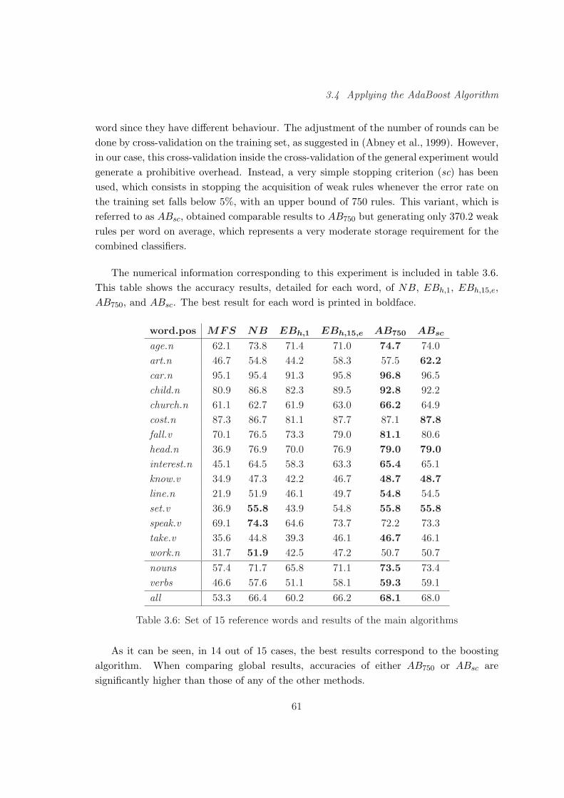
3.4 Applying the AdaBoost Algorithm
word since they have different behaviour. The adjustment of the number of rounds can bedone by cross-validation on the training set, as suggested in (Abney et al., 1999). However,in our case, this cross-validation inside the cross-validation of the general experiment wouldgenerate a prohibitive overhead. Instead, a very simple stopping criterion (sc) has beenused, which consists in stopping the acquisition of weak rules whenever the error rate onthe training set falls below 5%, with an upper bound of 750 rules. This variant, which isreferred to as ABsc, obtained comparable results to AB750 but generating only 370.2 weakrules per word on average, which represents a very moderate storage requirement for thecombined classifiers.
The numerical information corresponding to this experiment is included in table 3.6.This table shows the accuracy results, detailed for each word, of NB, EBh,1, EBh,15,e,AB750, and ABsc. The best result for each word is printed in boldface.
word.pos MFS NB EBh,1 EBh,15,e AB750 ABsc
age.n 62.1 73.8 71.4 71.0 74.7 74.0art.n 46.7 54.8 44.2 58.3 57.5 62.2car.n 95.1 95.4 91.3 95.8 96.8 96.5child.n 80.9 86.8 82.3 89.5 92.8 92.2church.n 61.1 62.7 61.9 63.0 66.2 64.9cost.n 87.3 86.7 81.1 87.7 87.1 87.8fall.v 70.1 76.5 73.3 79.0 81.1 80.6head.n 36.9 76.9 70.0 76.9 79.0 79.0interest.n 45.1 64.5 58.3 63.3 65.4 65.1know.v 34.9 47.3 42.2 46.7 48.7 48.7line.n 21.9 51.9 46.1 49.7 54.8 54.5set.v 36.9 55.8 43.9 54.8 55.8 55.8speak.v 69.1 74.3 64.6 73.7 72.2 73.3take.v 35.6 44.8 39.3 46.1 46.7 46.1work.n 31.7 51.9 42.5 47.2 50.7 50.7nouns 57.4 71.7 65.8 71.1 73.5 73.4verbs 46.6 57.6 51.1 58.1 59.3 59.1all 53.3 66.4 60.2 66.2 68.1 68.0
Table 3.6: Set of 15 reference words and results of the main algorithms
As it can be seen, in 14 out of 15 cases, the best results correspond to the boostingalgorithm. When comparing global results, accuracies of either AB750 or ABsc aresignificantly higher than those of any of the other methods.
61

3 A Comparison of Supervised ML Algorithms for WSD
Accelerating Boosting for WSD
Up to now, it has been seen that AdaBoost.MH is a simple and competitive algorithmfor the WSD task. It achieves an accuracy performance superior to that of the NaiveBayes and Exemplar-based baselines. However, AdaBoost.MH has the drawback of itscomputational cost, which makes the algorithm not scale properly to real WSD domainsof thousands of words.
The space and time-per-round requirements of AdaBoost.MH are O(mk) (recall thatm is the number of training examples and k the number of senses), not including the callto the weak learner. This cost is unavoidable since AdaBoost.MH is inherently sequential.That is, in order to learn the (t+1)-th weak rule it needs the calculation of the t-th weakrule, which properly updates the matrix Dt. Further, inside the WeakLearner, there isanother iterative process that examines, one by one, all attributes so as to decide whichis the one that minimises Zt. Since there are thousands of attributes, this is also a timeconsuming part, which can be straightforwardly speed up either by reducing the numberof attributes or by relaxing the need to examine all attributes at each iteration.
Four methods have been tested in order to reduce the cost of searching for weak rules.The first three, consisting of aggressively reducing the feature space, are frequently appliedin Text Categorisation. The fourth consists in reducing the number of attributes that areexamined at each round of the boosting algorithm.
• Frequency filtering (Freq): This method consists of simply discarding thosefeatures corresponding to events that occur less than N times in the training corpus.The idea beyond that criterion is that frequent events are more informative thanrare ones and unfrequent features may lead to overfitting.
• Local frequency filtering (LFreq): This method works similarly to Freq butconsiders the frequency of events locally, at the sense level. More particularly, itselects the N most frequent features of each sense and merging.
• RLM ranking: This third method consists in making a ranking of all attributesaccording to the RLM distance measure (de Mantaras, 1991) and selecting the N
most relevant features. This measure has been commonly used for attribute selectionin decision tree induction algorithms15.
15RLM distance belongs to the distance-based and information-based families of attribute selection
functions. It has been selected because it showed better performance than seven other alternatives in an
experiment of decision tree induction for POS tagging (Marquez, 1999).
62

3.4 Applying the AdaBoost Algorithm
• LazyBoosting: The last method does not filter out any attribute but reduces thenumber of those that are examined at each iteration of the boosting algorithm.More specifically, a small proportion p of attributes are randomly selected and thebest weak rule is selected among them. The idea behind this method is that if theproportion p is not too small, probably a sufficiently good rule can be found at eachiteration. Besides, the chance for a good rule to appear in the whole learning processis very high. Another important characteristic is that no attribute needs to bediscarded and so we avoid the risk of eliminating relevant attributes. This approachhas a main drawback: boosting changes the weight distribution at each iteration.Perhaps a good feature will loose importance at the iteration is selected due to thisweight distribution. Because this feature can be not important to the exampleswith highest weight. This method will be called LazyBoosting in reference to thework by Samuel and colleagues (Samuel, 1998). They applied the same techniquefor accelerating the learning algorithm in a Dialogue Act tagging system.
The four methods above have been compared for the set of 15 reference words. Figure3.5 contains the average error-rate curves obtained by the four variants at increasinglevels of attribute reduction. The top horizontal line corresponds to the MFS error rate,while the bottom horizontal line stands for the error rate of AdaBoost.MH working withall attributes. The results contained in figure 3.5 are calculated running the boostingalgorithm 250 rounds for each word.
The main conclusions that can be drawn are the following:
• All methods seem to work quite well since no important degradation is observed inperformance for values lower than 95% in rejected attributes. This may indicatethat there are many irrelevant or highly dependent attributes in our domain; andthat concepts depend only on a small set of features. All attribute filtering methodscapture the really important features.
• LFreq is slightly better than Freq, indicating a preference to make frequency countsfor each sense rather than globally.
• The more informed RLM ranking performs better than frequency-based reductionmethods Freq and LFreq.
• LazyBoosting is better than all other methods, confirming our expectations: it isworth keeping all information provided by the features. In this case, acceptableperformance is obtained even if only 1% of the attributes is explored when lookingfor a weak rule. The value of 10%, for which LazyBoosting still achieves the same
63

3 A Comparison of Supervised ML Algorithms for WSD
32
34
36
38
40
42
44
46
48
86 88 90 92 94 96 98 100
Err
or r
ate
(%)
Rejected attributes (%)
FreqLFreqRLM
LazyBoosting
Figure 3.5: Error rate obtained by the four methods, at 250 weak rules per word, withrespect to the percentage of rejected attributes
performance and runs about 7 times faster than AdaBoost.MH working with allattributes, will be selected for the experiments in next section.
Evaluating LazyBoosting
The LazyBoosting algorithm has been tested on the full DSO (all 191 words) with p = 10%and the same stopping criterion described above, which will be referred to as ABl10sc.
The ABl10sc algorithm learned an average of 381.1 rules per word, and took about4 days of cpu time to complete16. It has to be noted that this time includes thecross-validation overhead. Eliminating it, it is estimated that 4 cpu days would be thenecessary time for acquiring a word sense disambiguation boosting-based system coveringabout 2,000 words.
The ABl10sc has been compared again to the benchmark algorithms using the 10-foldcross-validation methodology described in section 3.2. The average accuracy results arereported in the upper-side of table 3.7. The best figures correspond to the LazyBoosting
16The implementation was written in PERL-5.003 and it was run on a SUN UltraSparc2 machine with
194Mb of RAM.
64
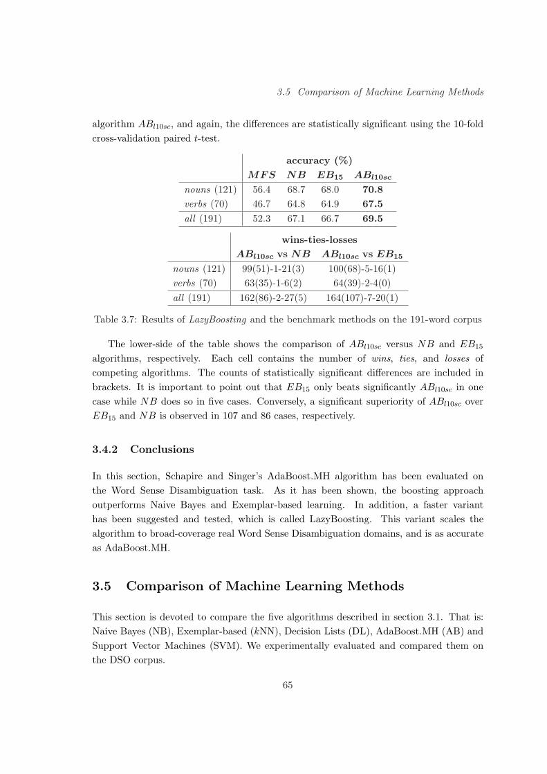
3.5 Comparison of Machine Learning Methods
algorithm ABl10sc, and again, the differences are statistically significant using the 10-foldcross-validation paired t-test.
accuracy (%)MFS NB EB15 ABl10sc
nouns (121) 56.4 68.7 68.0 70.8verbs (70) 46.7 64.8 64.9 67.5all (191) 52.3 67.1 66.7 69.5
wins-ties-lossesABl10sc vs NB ABl10sc vs EB15
nouns (121) 99(51)-1-21(3) 100(68)-5-16(1)verbs (70) 63(35)-1-6(2) 64(39)-2-4(0)all (191) 162(86)-2-27(5) 164(107)-7-20(1)
Table 3.7: Results of LazyBoosting and the benchmark methods on the 191-word corpus
The lower-side of the table shows the comparison of ABl10sc versus NB and EB15
algorithms, respectively. Each cell contains the number of wins, ties, and losses ofcompeting algorithms. The counts of statistically significant differences are included inbrackets. It is important to point out that EB15 only beats significantly ABl10sc in onecase while NB does so in five cases. Conversely, a significant superiority of ABl10sc overEB15 and NB is observed in 107 and 86 cases, respectively.
3.4.2 Conclusions
In this section, Schapire and Singer’s AdaBoost.MH algorithm has been evaluated onthe Word Sense Disambiguation task. As it has been shown, the boosting approachoutperforms Naive Bayes and Exemplar-based learning. In addition, a faster varianthas been suggested and tested, which is called LazyBoosting. This variant scales thealgorithm to broad-coverage real Word Sense Disambiguation domains, and is as accurateas AdaBoost.MH.
3.5 Comparison of Machine Learning Methods
This section is devoted to compare the five algorithms described in section 3.1. That is:Naive Bayes (NB), Exemplar-based (kNN), Decision Lists (DL), AdaBoost.MH (AB) andSupport Vector Machines (SVM). We experimentally evaluated and compared them onthe DSO corpus.
65
3 A Comparison of Supervised ML Algorithms for WSD
3.5.1 Setting of Evaluation
From the 191 words represented in the DSO corpus, a group of 21 words which frequentlyappear in the WSD literature has been selected to perform the comparative experiment.These words are 13 nouns (age, art, body, car, child, cost, head, interest, line, point, state,thing, work) and 8 verbs (become, fall, grow, lose, set, speak, strike, tell) and they havebeen treated as independent classification problems. The number of examples per wordranges from 202 to 1,482 with an average of 801.1 examples per word (840.6 for nouns and737.0 for verbs). The level of ambiguity is quite high in this corpus. The number of sensesis between 3 and 25, with an average of 10.1 senses per word (8.9 for nouns and 12.1 forverbs).
This comparison has SetB as feature set (see section 3.2.2). The different methodstested translate this information into features in different ways. The AdaBoost and SVMalgorithms require binary features. Therefore, local context attributes have to be binarisedin a preprocess, while the topical context attributes remain as binary tests about thepresence or absence of a concrete word in the sentence. As a result of this binarisation,the number of features is expanded to several thousands (from 1,764 to 9,900 dependingon the particular word).
The binary representation of features is not appropriate for Naive Bayes and kNNalgorithms. Therefore, the 15 local-context attributes are considered straightforwardly.Regarding the binary topical-context attributes, the variants described in section 3.3 areconsidered. For kNN, the topical information is codified as a single set-valued attribute(containing all words appearing in the sentence) and the calculation of closeness is modifiedso as to handle this type of attributes. For Naive Bayes, the topical context is conservedas binary features, but when classifying new examples only the information of wordsappearing in the example (positive information) is taken into account.
Regarding to kNN, we do not use MVDM here for simplicity reasons. Itsimplementation has a very serious computational overhead and the difference inperformance is reduced when using the Hamming distance jointly with feature and exampleweighting, as we do in this setting (see section 3.3).
We have performed a 10-fold cross-validation experiment in order to estimate theperformance of the systems. The accuracy figures reported below are (micro) averagedover the results of the 10 folds and over the results on each of the 21 words. We have applieda statistical test of significance, which is a paired Student’s t-test with a confidence valueof t9,0.995=3.250 (see appendix A for all the formulae about evaluation). When classifyingtest examples, all methods are forced to output a unique sense, resolving potential tiesbetween senses by choosing the most frequent sense among all those tied.
66
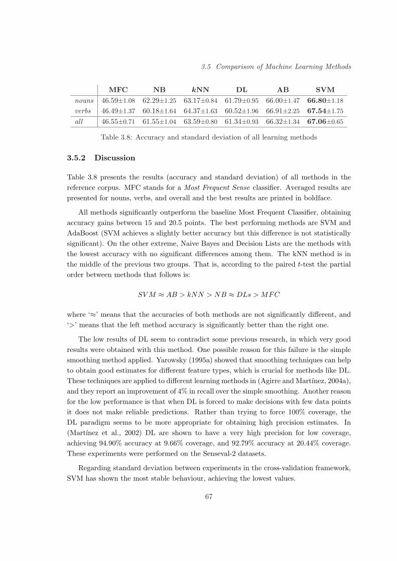
3.5 Comparison of Machine Learning Methods
MFC NB kNN DL AB SVMnouns 46.59±1.08 62.29±1.25 63.17±0.84 61.79±0.95 66.00±1.47 66.80±1.18
verbs 46.49±1.37 60.18±1.64 64.37±1.63 60.52±1.96 66.91±2.25 67.54±1.75
all 46.55±0.71 61.55±1.04 63.59±0.80 61.34±0.93 66.32±1.34 67.06±0.65
Table 3.8: Accuracy and standard deviation of all learning methods
3.5.2 Discussion
Table 3.8 presents the results (accuracy and standard deviation) of all methods in thereference corpus. MFC stands for a Most Frequent Sense classifier. Averaged results arepresented for nouns, verbs, and overall and the best results are printed in boldface.
All methods significantly outperform the baseline Most Frequent Classifier, obtainingaccuracy gains between 15 and 20.5 points. The best performing methods are SVM andAdaBoost (SVM achieves a slightly better accuracy but this difference is not statisticallysignificant). On the other extreme, Naive Bayes and Decision Lists are the methods withthe lowest accuracy with no significant differences among them. The kNN method is inthe middle of the previous two groups. That is, according to the paired t-test the partialorder between methods that follows is:
SV M ≈ AB > kNN > NB ≈ DLs > MFC
where ‘≈’ means that the accuracies of both methods are not significantly different, and‘>’ means that the left method accuracy is significantly better than the right one.
The low results of DL seem to contradict some previous research, in which very goodresults were obtained with this method. One possible reason for this failure is the simplesmoothing method applied. Yarowsky (1995a) showed that smoothing techniques can helpto obtain good estimates for different feature types, which is crucial for methods like DL.These techniques are applied to different learning methods in (Agirre and Martınez, 2004a),and they report an improvement of 4% in recall over the simple smoothing. Another reasonfor the low performance is that when DL is forced to make decisions with few data pointsit does not make reliable predictions. Rather than trying to force 100% coverage, theDL paradigm seems to be more appropriate for obtaining high precision estimates. In(Martınez et al., 2002) DL are shown to have a very high precision for low coverage,achieving 94.90% accuracy at 9.66% coverage, and 92.79% accuracy at 20.44% coverage.These experiments were performed on the Senseval-2 datasets.
Regarding standard deviation between experiments in the cross-validation framework,SVM has shown the most stable behaviour, achieving the lowest values.
67

3 A Comparison of Supervised ML Algorithms for WSD
<35 35-60 60-120 120-200 >200AB 60.19% 57.40% 70.21% 65.23% 73.93%SVM 63.59% 60.18% 70.15% 64.93% 72.90 %
Table 3.9: Overall accuracy of AB and SVM classifiers by groups of words of increasingaverage number of examples per sense
In this corpus subset, the average accuracy values achieved for nouns and verbs arevery close, being the baseline MFC results almost identical (46.59% for nouns and 46.49%for verbs). This is quite different from the results reported in many papers taking intoaccount the whole set of 191 words of the DSO corpus. For instance, differences between3 and 4 points can be observed in favour of nouns in previous section. This is due to thesingularities of the subset of 13 nouns studied here, which are particularly difficult. Notethat in the whole DSO corpus the MFC over nouns (56.4%) is fairly higher than in thissubset (46.6%) and that an AdaBoost-based system is able to achieve 70.8% on nounsin previous section compared to the 66.0% in this section. Also, the average number ofsenses per noun is higher than in the entire corpus. Despite this fact, a difference betweentwo groups of methods can be observed regarding the accuracy on nouns and verbs. Onthe one hand, the worst performing methods (NB and DLs) do better on nouns than onverbs. On the other hand, the best performing methods (kNN, AB, and SVM) are able tobetter learn the behaviour of verb examples, achieving an accuracy value around 1 pointhigher than for nouns.
Some researchers, Schapire (2002) for instance, argue that the AdaBoost algorithm mayperform very poorly when training using small samples. In order to verify this statementin the present study we calculated the accuracy obtained by AdaBoost in several groupsof words sorted by increasing size of training set. The size of a training set is taken as theratio between the number of examples and the number of senses of that word, that is, theaverage number of examples per sense. Table 3.9 shows the results obtained, includinga comparison with the SVM method. As expected, the accuracy of SVM is significantlysuperior than that of AdaBoost for small training sets (up to 60 examples per sense). Onthe contrary, AdaBoost outperforms SVM in the large training sets (over 120 examplesper sense). Recall that the overall accuracy is comparable in both classifiers (see table3.8).
In absolute terms, the overall results of all methods can be considered quite low(61-67%). We do not claim that these results can not be improved by using richer featurerepresentations, by a more accurate tuning of the systems, or by the addition of moretraining examples. Additionally, it is known that the DSO words included in this study areamong the most polysemous English words and that WordNet is a very fine-grained sense
68

3.5 Comparison of Machine Learning Methods
DSO MFC NB kNN DL AB SVMDSO – 46.6 61.5 63.6 61.3 66.3 67.1MFC -0.19 – 73.9 58.9 64.9 54.9 57.3NB 0.24 -0.09 – 75.2 76.7 71.4 76.7kNN 0.39 -0.15 0.43 – 70.2 72.3 78.0DL 0.31 -0.13 0.39 0.40 – 69.9 72.5AB 0.44 -0.17 0.37 0.50 0.42 – 80.3SVM 0.44 -0.16 0.49 0.61 0.45 0.65 –
Table 3.10: Kappa statistic (below diagonal) and percentage of agreement (above diagonal)between all pairs of systems on the DSO corpus
repository. Supposing that we had enough training examples for every ambiguous word inthe language, it is reasonable to think that a much more accurate all-words system couldbe constructed based on the current supervised technology. However, this assumption istotally unrealistic and, actually, the best current supervised systems for English all-wordsdisambiguation achieve figures around 65% (see Senseval-3 results). Our opinion is thatstate-of-the-art supervised systems still have to be qualitatively improved in order to bereally practical.
Apart from accuracy figures, the observation of the predictions made by the classifiersprovides interesting information about the comparison between methods. Table 3.10presents the percentage of agreement and the Kappa statistic between all pairs of systemson the test sets. ‘DSO’ stands for the annotation of the DSO corpus, which is taken asthe correct annotation. Therefore, the agreement rates with respect to DSO contain theaccuracy results previously reported. The Kappa statistic (Cohen, 1960) is a measureof inter-annotator agreement, which reduces the effect of chance agreement, and whichhas been used for measuring inter-annotator agreement during the construction of somesemantically annotated corpora (Veronis, 1998; Ng et al., 1999). A Kappa value of1 indicates perfect agreement, values around 0.8 are considered to indicate very goodagreement (Carletta, 1996), and negative values are interpreted as systematic disagreementon non-frequent cases.
NB obtains the most similar results with regard to MFC in agreement rate and Kappavalue. A 73.9% of agreement means that almost 3 out of 4 times it predicts the mostfrequent sense (which is correct in less than half of the cases). SVM and AB obtain themost similar results with regard to DSO (the manual annotation) in agreement rate andKappa values, and they have the less similar Kappa and agreement values with regard toMFC. This indicates that SVM and AB are the methods that best learn the behaviour ofthe DSO examples. It is also interesting to note that the three highest values of kappa
69

3 A Comparison of Supervised ML Algorithms for WSD
(0.65, 0.61, and 0.50) are between the top performing methods (SVM, AB, and kNN), andthat, despite NB and DLs achieve a very similar accuracy on the corpus, their predictionsare quite different, since the Kappa value between them is one of the lowest (0.39).
The Kappa values between the methods and the DSO annotation are very low. But,as it is suggested in (Veronis, 1998), evaluation measures should be computed relative tothe agreement between the human annotators of the corpus and not to a theoretical 100%.It seems pointless to expect more agreement between the system and the reference corpusthan between the annotators themselves. Contrary to the intuition that the agreementbetween human annotators could be very high in the Word Sense Disambiguation task,some papers report surprisingly low figures. For instance, Ng et al. (1999) report anaccuracy rate of 56.7% and a Kappa value of 0.317 when comparing the annotation ofa subset of the DSO corpus performed by two independent research groups. Similarly,Veronis (1998) reports values of Kappa near to zero when annotating some special wordsfor the ROMANSEVAL17 corpus.
From this point of view, the Kappa value of 0.44 achieved by SVM and AB could beconsidered pretty high result. Unfortunately, the subset of the DSO corpora treated inthis work does not coincide to that in (Ng et al., 1999) and, therefore, a direct comparisonis not possible.
3.6 Conclusions
In section 3.5 a comparison between five of the State-of-the-Art algorithms used in theWord Sense Disambiguation task have been performed. The systems’ performance hasbeen compared in terms of accuracy, but other measures, agreement and kappa valuesbetween each pair of methods, have been used to compare systems’ outputs. With allthis data a deeper study of the behaviour of the algorithms is possible. Among thefive algorithms compared, the best performing algorithms (in terms of accuracy andbehaviour on all senses to be learned) for the Word Sense Disambiguation task are bothAdaBoost.MH and Support Vector Machines: SVM for training sets with small numberof examples per sense (up to 60) and AdaBoost for larger sets (over 120). Up to now,there is no large sense-tagged corpus available. So, probably the best system could be acombination of both systems, depending on the number of examples per sense for eachword. That is, train each word with one of the algorithms depending on the number ofexamples per sense.
17http://www.lpl.univ-aix.fr/projectes/romanseval
70
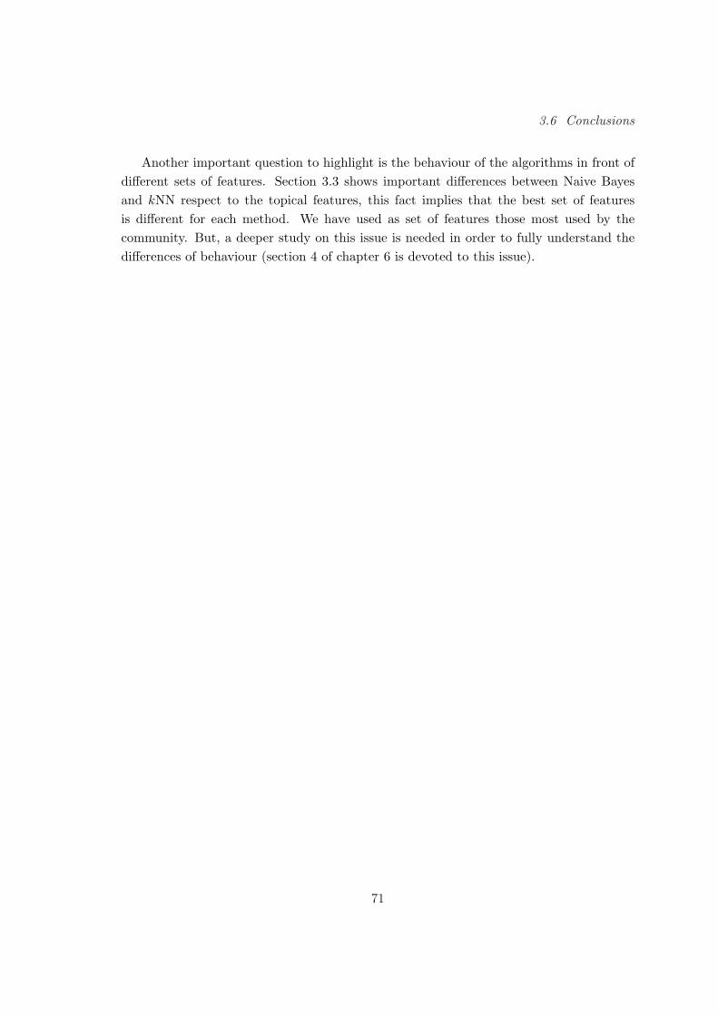
3.6 Conclusions
Another important question to highlight is the behaviour of the algorithms in front ofdifferent sets of features. Section 3.3 shows important differences between Naive Bayesand kNN respect to the topical features, this fact implies that the best set of featuresis different for each method. We have used as set of features those most used by thecommunity. But, a deeper study on this issue is needed in order to fully understand thedifferences of behaviour (section 4 of chapter 6 is devoted to this issue).
71

3 A Comparison of Supervised ML Algorithms for WSD
72

Chapter 4
Domain Dependence
This chapter describes a set of experiments carried out to explore the domain dependenceof alternative supervised Word Sense Disambiguation algorithms. The aim of the work is:studying the performance of these algorithms when tested on a different corpus from thatthey were trained on; and exploring their ability to tune to new domains. As we will see,the domain dependence of Word Sense Disambiguation systems seems very strong andsuggests that some kind of adaptation or tuning is required for cross-corpus applications.
4.1 Introduction
Supervised learning assumes that the training examples are somehow reflective of the taskthat will be performed by the trainee on other data. Consequently, the performance ofsuch systems is commonly estimated by testing the algorithm on a separate part of theset of training examples (say 10-20% of them), or by N -fold cross-validation, in whichthe set of examples is partitioned into N disjoint sets (or folds), and the training-testprocedure is repeated N times using all combinations of N−1 folds for training and 1fold for testing. In both cases, test examples are different from those used for training,but they belong to the same corpus, and, therefore, they are expected to be quite similar.Although this methodology could be valid for certain NLP problems, such as EnglishPart-of-Speech tagging, we think that there exists reasonable evidence to say that, inWSD, accuracy results cannot be simply extrapolated to other domains (contrary to theopinion of other authors Ng (1997b)): On the one hand, WSD is very dependant to thedomain of application Gale et al. (1992a) –see also Ng and Lee (1996); Ng (1997a), inwhich quite different accuracy figures are obtained when testing an exemplar-based WSDclassifier on two different corpora. On the other hand, it does not seem reasonable to
73

4 Domain Dependence
think that the training material can be large and representative enough to cover “all”potential types of examples. We think that an study of the domain dependence of WSD–in the style of other studies devoted to parsing Sekine (1997)– is needed to assess thevalidity of the supervised approach, and to determine to which extent a tuning process isnecessary to make real WSD systems portable to new corpora. In order to corroborate theprevious hypotheses, this chapter explores the portability and tuning of four different MLalgorithms (previously applied to WSD) by training and testing them on different corpora.Additionally, supervised methods suffer from the “knowledge acquisition bottleneck” Galeet al. (1992b). Ng (1997b) estimates that the manual annotation effort necessary to builda broad coverage semantically annotated English corpus is about 16 person-years. Thisoverhead for supervision could be much greater if a costly tuning procedure is requiredbefore applying any existing system to each new domain.
Due to this fact, recent works have focused on reducing the acquisition cost as wellas the need for supervision in corpus-based methods. It is our belief that the research byLeacock et al. (1998); Mihalcea and Moldovan (1999b)1 provide enough evidence towardsthe “opening” of the bottleneck in the near future. For that reason, it is worth furtherinvestigating the robustness and portability of existing supervised ML methods to betterresolve the WSD problem. It is important to note that the focus of this work will be on theempirical cross-corpus evaluation of several ML supervised algorithms. Other importantissues, such as: selecting the best attribute set, discussing an appropriate definition ofsenses for the task, etc., are not addressed in this chapter.
4.2 Setting
The set of comparative experiments has been carried out on a subset of 21 words of theDSO corpus. Each word is treated as a different classification problem. They are 13 nouns(age, art, body, car, child, cost, head, interest, line, point, state, thing, work) and 8 verbs(become, fall, grow, lose, set, speak, strike, tell)2. The average number of senses per wordis close to 10 and the number of training examples is close to 1,000.
The DSO corpus contains sentences from two different corpora. The first is Wall StreetJournal (WSJ), which belongs to the financial domain and the second is Brown Corpus(BC) being a general corpora of English usage. Therefore, it is easy to perform experimentsabout the portability of alternative systems by training them on the WSJ part (A part,hereinafter) and testing them on the BC part (B part, hereinafter), or vice-versa.
1In the line of using lexical resources and search engines to automatically collect training examples from
large text collections or the Web.2This set of words is the same used in the final comparison of the previous chapter (section 3.5).
74

4.3 First Experiment: Across Corpora evaluation
Two kinds of information are used to train classifiers: local and topical context. Theformer consists of the words and part-of-speech tags appearing in a window of ± 3 itemsaround the target word, and collocations of up to three consecutive words in the samewindow. The latter consists of the unordered set of content words appearing in the wholesentence3.
The four methods tested (Naive Bayes, Exemplar-Based, Decision Lists, andLazyBoosting) translate this information into features in different ways. LazyBoostingalgorithm requires binary features. Therefore, local context attributes have to be binarisedin a preprocess, while the topical context attributes remain as binary tests about thepresence/absence of a concrete word in the sentence. As a result the number of attributesis expanded to several thousands (from 1,764 to 9,900 depending on the particularword). The binary representation of attributes is not appropriate for Naive Bayesand Exemplar-Based algorithms. Therefore, the 15 local-context attributes are takenstraightforwardly. Regarding the binary topical-context attributes, we have used thevariants described in chapter 3. For Exemplar-Based, the topical information is codifiedas a single set-valued attribute (containing all words appearing in the sentence) and thecalculation of the closeness measure is modified so as to handle this type of attribute. ForNaive Bayes, the topical context is conserved as binary features, but when classifying newexamples only the information of words appearing in the example (positive information)is taken into account.
4.3 First Experiment: Across Corpora evaluation
The comparison of algorithms has been performed in series of controlled experiments usingexactly the same training and test sets. There are 7 combinations of training-test setscalled: A+B→A+B, A+B→A, A+B→B, A→A, B→B, A→B, and B→B, respectively. Inthis notation, the training set is placed at the left hand side of symbol “→”, while the testset is at the right hand side. For instance, A→B means that the training set is corpus A andthe test set is corpus B. The symbol “+” stands for set union, therefore A+B→B meansthat the training set is A union B and the test set is B. When comparing the performanceof two algorithms, two different statistical tests of significance have been applied dependingon the case. A→B and B→A combinations represent a single training-test experiment.In this cases, the McNemar’s test of significance is used (with a confidence value of:χ2
1,0.95 = 3.842), which is proven to be more robust than a simple test for the difference oftwo proportions. In the other combinations, a 10-fold cross-validation was performed in
3This set of features is the SetB defined in section 3.2.2.
75

4 Domain Dependence
order to prevent testing on the same material used for training. The associated statisticaltests of significance is a paired Student’s t-test with a confidence value of: t9,0.975 = 2.262(see appendix A for evaluation formulae).
The four algorithms, jointly with a naive Most-Frequent-sense Classifier (MFC), havebeen tested on 7 different combinations of training-test sets. Accuracy figures, averagedover the 21 words, are reported in table 4.1. The comparison leads to the followingconclusions:
MFC NB EB DL LBA+B→A+B 46.55±0.71 61.55±1.04 63.01±0.93 61.58±0.98 66.32±1.34
A+B→A 53.90±2.01 67.25±1.07 69.08±1.66 67.64±0.94 71.79±1.51
A+B→B 39.21±1.90 55.85±1.81 56.97±1.22 55.53±1.85 60.85±1.81
A→A 55.94±1.10 65.86±1.11 68.98±1.06 67.57±1.44 71.26±1.15
B→B 45.52±1.27 56.80±1.12 57.36±1.68 56.56±1.59 58.96±1.86
A→B 36.40 41.38 45.32 43.01 47.10B→A 38.71 47.66 51.13 48.83 51.99∗
Table 4.1: Accuracy results (± standard deviation) of the methods on all training-testcombinations
• LazyBoosting outperforms all other methods in all cases. Additionally, thissuperiority is statistically significant, except when comparing LazyBoosting to theExemplar-Based approach in 5 of the 21 cases.
• Surprisingly, LazyBoosting in A+B→A (or A+B→B) does not achieve substantialimprovement to the results of A→A (or B→B). Actually, the first variation isnot statistically significant and the second is only slightly significant. That is, theaddition of extra examples from another domain does not necessarily contribute toimprove the results on the original corpus.
• Regarding the portability of the systems, very disappointing results are obtained.Restricting to LazyBoosting results, we observe that the accuracy obtained in A→B is47.1% while the accuracy in B→B (which can be considered an upper bound forLazyBoosting in B corpus) is 59.0%, that is, a drop of 12 points. Furthermore,47.1% is only slightly better than the most frequent sense in corpus B, 45.5%. Thecomparison in the reverse direction is even worse: a drop from 71.3% (A→A) to52.0% (B→A), which is lower than the most frequent sense of corpus A, 55.9%.
76

4.4 Second Experiment: tuning to new domains
4.4 Second Experiment: tuning to new domains
The previous experiment shows that classifiers trained on the A corpus do not work wellon the B corpus, and vice-versa. Therefore, it seems that some kind of tuning processis necessary to adapt supervised systems to each new domain. This experiment exploresthe effect of a simple tuning process consisting of adding to the original training set arelatively small sample of manually sense tagged examples of the new domain. The sizeof this supervised portion varies from 10% to 50% of the available corpus in steps of 10%(the remaining 50% is kept for testing). This set of experiments will be referred to asA+%B→B, or conversely, B+%A→A.
In order to determine to which extent the original training set contributes to accuratelydisambiguate in the new domain, we also calculate the results for %A→A (and %B→B),that is, using only the tuning corpus for training.
Figure 4.1 graphically presents the results obtained by all methods. Each plot containsX+%Y→Y and %Y→Y curves, and the straight lines corresponding to the lower boundMFC, and to the upper bounds Y→Y and X+Y→Y .
As expected, the accuracy of all methods grows (towards the upper bound) as moretuning corpus is added to the training set. However, the relation between X+%Y→Y and%Y→Y reveals some interesting facts. In plots 1b, 2a, and 3b the contribution of theoriginal training corpus is almost negligible. Furthermore, in plots 1a, 2b, and 3a adegradation on the accuracy performance is observed. Summarising, these six plots showthat for Naive Bayes, Exemplar-Based and Decision Lists methods it is not worth keepingthe original training examples. Instead, a better (but disappointing) strategy would besimply using the tuning corpus.
However, this is not the situation of LazyBoosting (plots 4a and 4b), for whicha moderate (but consistent) improvement of accuracy is observed when retaining theoriginal training set. Therefore, LazyBoosting shows again a better behaviour than theircompetitors when moving from one domain to another.
4.5 Third Experiment: training data quality
The bad results about portability may be explained by, at least, two reasons: 1) CorpusA and B have a very different distribution of senses, and, therefore, different a-prioribiases; 2) Examples of corpus A and B contain different information, and, therefore, thelearning algorithms acquire different (and non interchangeable) classification cues fromboth corpora.
77

4 Domain Dependence
(1a) NB on A (1b) NB on B
40
42
44
46
48
50
52
54
56
58
0 5 10 15 20 25 30 35 40 45 50
Acc
urac
y ra
te (
%)
MFSB-B
A+B-BA+%B-B
%B-B
54
56
58
60
62
64
66
68
70
72
0 5 10 15 20 25 30 35 40 45 50
Acc
urac
y ra
te (
%)
MFSA-A
A+B-AA+%B-A
%A-A
(2a) EB on A (2b) EB on B
44
46
48
50
52
54
56
58
0 5 10 15 20 25 30 35 40 45 50
Acc
urac
y ra
te (
%)
MFSB-B
A+B-BA+%B-B
%B-B
54
56
58
60
62
64
66
68
70
72
0 5 10 15 20 25 30 35 40 45 50
Acc
urac
y ra
te (
%)
MFSA-A
A+B-AA+%B-A
%A-A
(3a) DL on A (3b) DL on B
42
44
46
48
50
52
54
56
58
0 5 10 15 20 25 30 35 40 45 50
Acc
urac
y ra
te (
%)
MFSB-B
A+B-BA+%B-B
%B-B
54
56
58
60
62
64
66
68
70
72
0 5 10 15 20 25 30 35 40 45 50
Acc
urac
y ra
te (
%)
MFSA-A
B+A-AB+%A-A
%A-A
(4a) LB on A (4b) LB on B
44
46
48
50
52
54
56
58
60
62
0 5 10 15 20 25 30 35 40 45 50
Acc
urac
y ra
te (
%)
MFSB-B
A+B-BA+%B-B
%B-B
54
56
58
60
62
64
66
68
70
72
0 5 10 15 20 25 30 35 40 45 50
Acc
urac
y ra
te (
%)
MFSA-A
A+B-AA+%B-A
%A-A
Figure 4.1: Results of the tuning experiment
78

4.5 Third Experiment: training data quality
The first hypothesis is confirmed by observing the bar plots of figure 4.2, which containthe distribution of the four most frequent senses of some sample words in the corpora A andB, respectively. In order to check the second hypothesis, two new sense-balanced corporahave been generated from the DSO corpus, by equilibrating the number of examples ofeach sense between A and B parts. In this way, the first difficulty is artificially overridedand the algorithms should be portable if examples of both parts are quite similar. Table4.2 shows the results obtained by LazyBoosting on these new corpora.
Figure 4.2: Distribution of the four most frequent senses for two nouns (head, interest)and two verbs (fall, grow). Black bars = A corpus; Grey bars = B corpus
Regarding portability, we observe a significant accuracy decrease of 7 and 5 pointsfrom A→A to B→A, and from B→B to A→B, respectively. This loss in accuracy is not asimportant as in the first experiment, due to the simplification provided by the balancingof sense distributions. That is, even when the same distribution of senses is conservedbetween training and test examples, the portability of the supervised WSD systems isnot guaranteed. These results imply that examples have to be largely different from onecorpus to another.
The observation of the rules acquired by LazyBoosting also could help improving dataquality. It is known that misslabelled examples resulting from annotation errors tend tobe hard examples to classify correctly, and, therefore, tend to have large weights in thefinal distribution. Abney et al. (1999) applied this idea from AdaBoost to PoS tagging,improving the data quality. This observation allows both to identify the noisy examplesand use LB as a way to improve the training corpus. An experiment has been carried
79

4 Domain Dependence
MFC LBA+B→A+B 48.55±1.16 64.35±1.16
A+B→A 48.64±1.04 66.20±2.12
A+B→B 48.46±1.21 62.50±1.47
A→A 48.62±1.09 65.22±1.50
B→B 48.46±1.21 61.74±1.18
A→B 48.70 56.12B→A 48.70 58.05
Table 4.2: Accuracy results (± standard deviation) of LazyBoosting on the sense-balancedcorpora
out in this direction by studying the rules acquired by LB from the training examples ofword state. The manually inspection of the 50 highest scored rules allowed us to identify ahigh number of noisy training examples -there were 11 tagging errors-, and, additionally,17 examples not coherently tagged, probably due to the too fine grained or not so cleardistinctions between the senses involved in these examples. Thus, there were 28 of 50examples with some kind of problem among the best scored.
See, for instance, the two rules presented in table 4.3, acquired from corpus A and B
respectively, which account for the collocation state court. For each rule and each sensethere are two real numbers, which are the rule outputs when the feature holds in theexample and when it does not, respectively. The sign of real numbers is interpreted as aprediction as to whether the sense should or should not be assigned to the example. Themagnitude of the prediction is interpreted as a measure of confidence in the prediction.Therefore, according to the first rule, the presence of the collocation state court givespositive evidence to the sense number 3 and negative to the rest of senses. On the contrary,according to the second rule the presence of such collocation would contribute to sensenumber 5 and negatively to all the rest (including sense number 3).
sensessource 0 1 2 3 4 5
rule 1 A -0.5064 -1.0970 -0.6992 1.2580 -1.0125 -0.47210.0035 0.0118 0.0066 -0.0421 0.0129 0.0070
rule 2 B -0.0696 -0.2988 -0.1476 -1.1580 -0.5095 1.2326-0.0213 0.0019 -0.0037 0.0102 0.0027 -0.0094
Table 4.3: Example of WeakRule: it is referred to the collocation state court
It has to be noted that these rules are completely coherent with the senses assigned
80

4.6 Conclusions
to the examples containing state court in both corpora, and therefore, the contradictioncomes from different information that characterise examples of both corpora.
4.6 Conclusions
This work has pointed out some difficulties regarding the portability of supervised WSDsystems, a very important issue that has been paid little attention up to the present.According to our experiments, it seems that the performance of supervised sense taggersis not guaranteed when moving from one domain to another (e.g. from a balanced corpus,such as BC, to an economic domain, such as WSJ). These results implies that somekind of adaptation is required for cross-corpus application. Furthermore, these resultsare in contradiction with the idea of “robust broad-coverage WSD” introduced by Ng(1997b), in which a supervised system trained on a large enough corpora (say a thousandexamples per word) should provide accurate disambiguation on any corpora (or, at leastsignificantly better than MFS). Consequently, it is our belief that a number of issuesregarding portability, tuning, knowledge acquisition, etc., should be thoroughly studiedbefore stating that the supervised ML paradigm is able to resolve a realistic WSD problem.Regarding the ML algorithms tested, the contribution of this work consist of empiricallydemonstrating that the LazyBoosting algorithm outperforms other three supervised MLmethods for WSD. Furthermore, this algorithm is proven to have better properties whenis applied to new domains.
81

4 Domain Dependence
82

Chapter 5
Bootstrapping
As we have seen in previous chapters, supervised systems are one of the most promisingapproaches to Word Sense Disambiguation. The most important drawback with them isthe need of a large quantity of labelled examples to train classifiers. One of the mostimportant open lines of research in the field is the use of bootstrapping techniques to takeadvantage of the unlabelled examples in learning classifiers. It is usually easy to obtainunlabelled examples from large resources, such as the Web or large text collections. Themain aim of this chapter is to explore the usefulness of unlabelled examples in SupervisedWord Sense Disambiguation systems. We explore in this chapter two approaches of thosedescribed in section 2.3.1: the transductive learning for SVMs (Joachims, 1999) and thebootstrapping algorithm proposed by Abney (2002, 2004).
5.1 Transductive SVMs
The Transductive approach (Vapnik, 1998) consists of training a system with labelledand unlabelled examples at a time. Specifically, the transductive approach for SupportVector Machines begins by learning a usual SVM from the labelled examples and ends byadjusting the separating hyperplane by means of an iterative process, guessing the classof the unlabelled examples. The proportion of examples for each class is being maintainedthroughout all iterations.
Joachims (1999) suggested the utility of the transductive approach for TextCategorisation. The experiments show the viability of training with a small set of labelledexamples and a large set of “cheap” unlabelled examples.
Word Sense Disambiguation and Text Categorisation share some importantcharacteristics: high dimensional input space, sparse example vectors and few irrelevant
83

5 Bootstrapping
features. The transductive approach seems to work well in Text Categorisation becausedocuments usually share words (treated as features) of the domain. That is, each domainor category has some typical words associated and the documents of the same categoryusually contain a subset of them. Once identifies with one of the categories, the unlabelledexamples are used to generalise the classification model with other complementary featuresnot included in the labelled set. See details at (Joachims, 1998, 1999). This section reportsthe experiment of Joachims (1999) ported to the Word Sense Disambiguation problem,using as data the DSO corpus.
5.1.1 Setting
The experiment have been carried out using the SV M light implementation of the Inductive(SV M) and Transductive (TSV M) Support Vector Machines. This software, developedby Thorsten Joachims (1999), is publicly available and open source.
For this work, eight words of the DSO corpus (Ng and Lee, 1996) have been selected.Seven of them have the higher number of examples in the DSO corpus. The other, art,has been selected because of the availability of a large unlabelled corpus for this word.They are 4 nouns (art, law, state, and system) and 4 verbs (become, leave, look, and think).Table 5.1 shows, as a reference, the number of examples, and the 10 fold cross-validationaccuracy of the naive Most Frequent Classifier and the implementation of AdaBoost.MHdescribed in section 3.4. The English version of FreeLing part-of-speech tagger have beenused for tagging (Atserias et al., 2006). The accuracy improvement over the MFC baselineis 21.7 points, comparable to those obtained in previous chapters.
Two partitions of examples have been generated. One of 10 folds (hereinafter PA)used for parameter tuning and one of 20 folds (hereinafter PB) for the main experiment.The examples have been randomly selected maintaining the proportion of the examplesper sense for each fold.
Feature Set
Let “. . . w−3 w−2 w−1 w w+1 w+2 w+3 . . .” be the context of consecutive words aroundthe word w to be disambiguated, and p±i (−3≤i≤3) be the part-of-speech tag of wordw±i. The feature patterns referring to local context are the following: w, p−3, p−2, p−1,p+1, p+2, p+3, w+3, w−2, w−1, w+1, w+2 and w+3.
The features referring to topical context consist of: the unordered set of open-classwords appearing in the sentence, all bigrams of open-class words (after deleting the
84

5.1 Transductive SVMs
word.pos #exs mfc boostart.n 388 46.7 61.0law.n 1,489 29.6 60.7state.n 1,438 33.7 46.5system.n 1,491 26.0 38.5become.v 1,455 40.5 68.2leave.v 1,471 29.7 50.1look.v 1,450 51.0 77.3think.v 1,442 46.1 69.5nouns 4,806 31.1 49.6verbs 5,818 41.8 66.2all 10,624 37.0 58.7
Table 5.1: Number of examples and accuracy results of the two baseline systems (in %)
closed-class words of the sentence), and, finally, all the word bigrams appearing in thesentence (including open- and closed-class words).
This feature set is a small modification of SetB in section 3.2.2. Local trigrams havebeen deleted and the topical bigrams added. This decision has been motivated due toexperimental results of Senseval exercises (see chapter 6).
Parameter Tuning
As in the previous chapters, one of the first things to decide when using the SupportVector Machines is the kernel. Simple linear SVMs have been used, since the use of morecomplex kernels (polynomials, gaussian functions, etc.) did not lead to better results insome exploratory experiments.
There is another parameter to estimate, the C value. This parameter measures thetrade-off between training error and margin maximisation. Table 5.2 contains the C valuefor the SVMs and TSVMs estimated in a 10–fold cross-validation experiment (over the PA
partition), by selecting the values maximising accuracy. The values ranged from 0 and 2.5in steps of 0.05. In previous experiments we have seen that good values for the parameterapplied to WSD data are those near to 0. In the SV M case, 9 folds are considered astraining set and 1 fold as testing set each time, while in the TSV M case, 1 fold is takenas the training set and the remaining 9 as test set, in order to better resemble the realusage scenario.
In performing the parameter tuning, there is another possible improvement to test.
85

5 Bootstrapping
C valueword SVM TSVMart.n 0.1 1.35law.n 0 0.05state.n 0 2.05system.n 0.05 1.25become.v 0.1 0.05leave.v 0.05 0.05look.v 0.05 0.05think.v 0 1.1
Table 5.2: Optimum values of parameter C
SV M light is a binary implementation of SVM. That is, it can not directly deal with amulticlass classification problem (see section 6.4 for some binarisation examples). In orderto provide a classifier for that kind of problems, a binarisation process have to be done.Thus, the parameter tuning can be done at the level of each of binary problem. However,first results in this direction showed no significant improvements.
5.1.2 Experiments with TSVM
There are two main experiments in Joachims (1999): the first one aiming to show theeffect of the training set size (fixing the size of the test set) and the other one to see theeffect of the test set size (fixing the training set to a small size).
Both experiments reported a better accuracy for the transductive approach than theinductive one, but not for all the classes. The first experiment showed largest differenceswhen using very small training sets, tending to disappear when increasing the numberof training examples. The second experiment showed a logarithmic-like accuracy curve,always over the accuracy result of the inductive approach.
Main Experiment
This section is devoted to translate experiments in (Joachims, 1999) to the Word SenseDisambiguation domain. It consists of carrying out two experiments for each problem.In this case, the PB partition of the corpus has been used. This experiment (hereinafterVarTrain) tries to show the effect of the number of examples in the training set, fixingthe test set; and, the second (hereinafter VarTest) the effect of the number of examplesin test set, fixing the training set.
86

5.1 Transductive SVMs
Figure 5.1 shows the results of these experiments for the 4 nouns considered, and figure5.2 for the 4 verbs. Left plots of both figures show the results of the VarTrain experiment,and right plots show the VarTest results. For better understanding, table 5.3 shows thefolds used as training and test sets in both experiments. VarTrain outputs a learningcurve in which the test set are always folds from 10 to 19 and the training set is variable.In the first iteration the training set is fold 0, in the second iteration, the training arefolds 0 and 1 and so on until using for training folds from 0 to 9. VarTest has the samebehaviour but fixing training set to fold 0, and varying test set from the use of only fold1, to the use of folds form 1 to 19.
VarTrain VarTestTraining Set Folds 0, 0-1, . . . , 0-9 Fold 0Testing Set Folds 10-19 Folds 1, 1-2, . . . , 1-19
Table 5.3: Number of folds used as training and test sets in each experiment
The learning curves are very disappointing. All VarTrain plots show worse performancefor TSVM than for SVM. Only in the case of the verb become the accuracy is comparable.VarTest plots show a very irregular behaviour, that in many cases tends to decrease theaccuracy when using TSVM. There is only a case (verb become) in which the results aresimilar to those observed in the Text Categorisation problem by Joachims.
Second Experiment
A second experiment has been conducted in order to test the integrity of the transductivemodels. It consists of running SVM and TSVM under the same conditions and with a smallnumber of examples in the test set (9 folds for training a 1 fold for test), for minimisingthe effect of the transductive examples.
The results of this experiment are shown in table 5.4. It can be seen that when using thetransductive approach the accuracy of the system decreases in all words. The parametershave been tuned over the inductive approach, but this is not a plausible reason for thecomparative low results of TSVM. In the experiments of Joachims (1999) the accuracyof TSVM is always higher than that of SVM. This fact is an evidence of the differencesbetween Text Categorisation and Word Sense Disambiguation problems.
Another evidence is the nature of examples in both problems. In Text Categorisationthe examples are documents and their representation usually consists of the words of thedocument, and the problem is to assign one or more labels to the document. In Word SenseDisambiguation the examples are sentences where a word has to be tagged with a sense
87

5 Bootstrapping
VarTrain VarTest
art.n
40
45
50
55
60
65
70
75
80
1 2 3 4 5 6 7 8 9 10
Acc
urac
y (%
)
Number of Training Folds
SVMTSVM
35
40
45
50
55
60
0 2 4 6 8 10 12 14 16 18 20
Acc
urac
y (%
)
Number of Transductive Folds
SVMTSVM
law.n
40
45
50
55
60
65
70
75
80
1 2 3 4 5 6 7 8 9 10
Acc
urac
y (%
)
Number of Training Folds
SVMTSVM
35
40
45
50
55
60
0 2 4 6 8 10 12 14 16 18 20
Acc
urac
y (%
)
Number of Transductive Folds
SVMTSVM
state.n
20
25
30
35
40
45
50
55
60
1 2 3 4 5 6 7 8 9 10
Acc
urac
y (%
)
Number of Training Folds
SVMTSVM
30
35
40
45
50
55
0 2 4 6 8 10 12 14 16 18 20
Acc
urac
y (%
)
Number of Transductive Folds
SVMTSVM
system.n
20
25
30
35
40
45
50
55
60
1 2 3 4 5 6 7 8 9 10
Acc
urac
y (%
)
Number of Training Folds
SVMTSVM
20
25
30
35
40
45
0 2 4 6 8 10 12 14 16 18 20
Acc
urac
y (%
)
Number of Transductive Folds
SVMTSVM
Figure 5.1: Main TSVM experiment on nouns
88

5.1 Transductive SVMs
VarTrain VarTest
become.v
50
55
60
65
70
75
80
85
90
1 2 3 4 5 6 7 8 9 10
Acc
urac
y (%
)
Number of Training Folds
SVMTSVM
55
60
65
70
75
80
0 2 4 6 8 10 12 14 16 18 20
Acc
urac
y (%
)
Number of Transductive Folds
SVMTSVM
leave.v
30
35
40
45
50
55
60
65
1 2 3 4 5 6 7 8 9 10
Acc
urac
y (%
)
Number of Training Folds
SVMTSVM
20
25
30
35
40
45
0 2 4 6 8 10 12 14 16 18 20
Acc
urac
y (%
)
Number of Transductive Folds
SVMTSVM
look.v
50
55
60
65
70
75
80
85
90
1 2 3 4 5 6 7 8 9 10
Acc
urac
y (%
)
Number of Training Folds
SVMTSVM
50
55
60
65
70
75
0 2 4 6 8 10 12 14 16 18 20
Acc
urac
y (%
)
Number of Transductive Folds
SVMTSVM
think.v
50
55
60
65
70
75
80
85
90
1 2 3 4 5 6 7 8 9 10
Acc
urac
y (%
)
Number of Training Folds
SVMTSVM
50
55
60
65
70
75
0 2 4 6 8 10 12 14 16 18 20
Acc
urac
y (%
)
Number of Transductive Folds
SVMTSVM
Figure 5.2: Main TSVM experiment on verbs
89
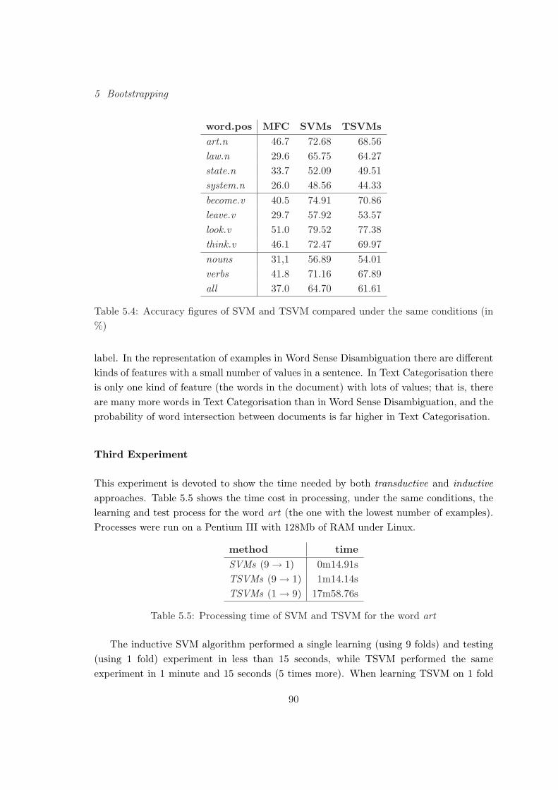
5 Bootstrapping
word.pos MFC SVMs TSVMsart.n 46.7 72.68 68.56law.n 29.6 65.75 64.27state.n 33.7 52.09 49.51system.n 26.0 48.56 44.33become.v 40.5 74.91 70.86leave.v 29.7 57.92 53.57look.v 51.0 79.52 77.38think.v 46.1 72.47 69.97nouns 31,1 56.89 54.01verbs 41.8 71.16 67.89all 37.0 64.70 61.61
Table 5.4: Accuracy figures of SVM and TSVM compared under the same conditions (in%)
label. In the representation of examples in Word Sense Disambiguation there are differentkinds of features with a small number of values in a sentence. In Text Categorisation thereis only one kind of feature (the words in the document) with lots of values; that is, thereare many more words in Text Categorisation than in Word Sense Disambiguation, and theprobability of word intersection between documents is far higher in Text Categorisation.
Third Experiment
This experiment is devoted to show the time needed by both transductive and inductiveapproaches. Table 5.5 shows the time cost in processing, under the same conditions, thelearning and test process for the word art (the one with the lowest number of examples).Processes were run on a Pentium III with 128Mb of RAM under Linux.
method timeSVMs (9 → 1) 0m14.91sTSVMs (9 → 1) 1m14.14sTSVMs (1 → 9) 17m58.76s
Table 5.5: Processing time of SVM and TSVM for the word art
The inductive SVM algorithm performed a single learning (using 9 folds) and testing(using 1 fold) experiment in less than 15 seconds, while TSVM performed the sameexperiment in 1 minute and 15 seconds (5 times more). When learning TSVM on 1 fold
90

5.2 Greedy Agreement Bootstrapping Algorithm
and testing over 9 folds the time requirements grow up to 18 minutes. As expected, theTSVM is very time consuming when a large amount of unlabelled examples are includedin the training process.
The high cost of TSVM is due to the need of retraining at every classificationof an unlabelled example. This cost could be alleviated by an incremental (on-line)implementation of the SVM paradigm, which is by now not available in the SV M light
software.
5.2 Greedy Agreement Bootstrapping Algorithm
This section describes an experiment carried out to explore the bootstrapping algorithm,described in (Abney, 2002, 2004), applied to Word Sense Disambiguation (see section2.3.1 for a discussion of the different bootstrapping algorithms). It consists of learningtwo views (independent classifiers) called F and G, respectively, and it is assumed thatboth are conditionally independent given a target label. In practice, both views F andG are classifiers that learn with the same ML algorithms but with different feature set.The bootstrapping algorithm is an iterative process (figure 5.3 shows its pseudo-code) thatlearns an atomic rule for one of the views at each iteration alternatively. The algorithmneeds as input a set of seeds, that is, an initial set of atomic rules with a very highprecision, but low coverage. The result of the learning process consists of two classifiers,one for each view, which may be combined to classify new instances.
procedure Greedy Agreement
Input: seed rules F, G
loopforeach atomic rule H
G′ := G + H
evaluate cost of (F, G′)keep lowest-cost G′
if G′ is worse than G, quit
swap F, G′
return F and G
end Greedy Agreement
Figure 5.3: The Greedy Agreement algorithm
Classifiers F and G induced from both views can abstain when predicting: F (x) = ⊥
91

5 Bootstrapping
or G(x) = ⊥. The cost function needed by the algorithm is defined in (Abney, 2002) as:
cost(F, G) =cost(F ) + cost(G)
2
wherecost(F ) =
δ
µ− δ× lab(F ) + unlab(F )
where δ = Pr[F 6= G|F, G 6= ⊥], µ = minuPr[F = u|F 6= ⊥], lab(F ) is the numberof predictions of classifier F , and unlab(F ) is the number of times classifier F abstains.cost(G) is computed in the same way.
Each atomic rule corresponds to test the value of a unique feature and emit aclassification decision. This algorithm does not delete atomic rules. That is, an atomicrule could be selected more than one time. This fact allows to assign some kind of “weight”to the atomic rules (or features).
Finally, the combination of both views, in order to get a final classification, is nota trivial issue due to the fact that both views could abstain or predict a label. Wehave implemented several alternatives that are tested in the subsequent experiments. Allvariants we tried are summarised in table 5.6 together with a brief explanation of eachstrategy.
5.2.1 Setting
Four words of the DSO corpus have been selected. These words have the highest numberof examples for their two most frequent senses. They are two nouns (law and system)and two verbs (become and think). Table 5.7 shows the two most frequent senses and thenumber of examples for each of these senses. The experiment has been performed takinginto account only these two most frequent senses for each word. Abney (2002) applied itsalgorithm to Name Entity Recognition and for that task he had available a very large dataset. In WSD there are not such a large annotated corpora. This is why we have selectedonly the two most frequent senses from those words with more examples.
Table 5.8 shows the set of features selected for each view and a short description ofeach feature. Considering the assumption of conditionally independence of the views, wehave chosen three local features for view F and three topical features for view G.
A random partition of examples in 10 folds has been generated. These folds have beennumbered from 0 to 9. Tables 5.9 and 5.10 show the results (precision, recall, F1 andcoverage) calculated to serve as baselines for nouns and verbs respectively. “0 → (1− 8)”stands for fold 0 as training data and folds from 1 to 8 as test data. “0 → 9” stands for
92

5.2 Greedy Agreement Bootstrapping Algorithm
key definitionSTRICT AGREE the final classifier only predicts a label (as output) if both
classifiers (F and G) have a prediction and the label is thesame
RELAX AGREE the final classifier predicts a label e if both classifiers F andG predict the same label e or if one predicts e and the otherabstains
PRIORITY X the final classifier predicts a label e if one or both predict e;but if both labels are different, it predicts that of view X;where X ∈ {F, G}
STRICT VOTING the final classifier only predicts a label when both classifiershave a prediction; then it gets the highest scoring label; elseabstains
RELAX VOTING STRICT VOTING but if one of the views abstains, the finalclassifier takes the label from the non abstaining view
ONLY VOTING the predicted label is the highest scoring label from bothclassifiers and all classes
Table 5.6: Description of the ways of combining both views
senses exampleslaw.n 14:00 10:00 444 361system.n 06:00 09:02 417 141become.v 30:00 42:00 606 532think.v 31:01 31:00 690 429
Table 5.7: Senses and number of examples for each word selected from DSO corpus
view feature descriptionF bigsf all word form bigrams in the sentenceF fcomb word forms of all pairs (consecutive or not) of the
open-class-words in the sentenceF top f bag of word forms of the sentenceG f loc all word forms and its position in a ±3-word-windowG form word form of the target wordG p loc part-of-speech of the relative words in a ±3-word-window
together with their position to the target word
Table 5.8: Description of the features for each view
93

5 Bootstrapping
fold 0 as training data and fold 9 as test data. The distribution of the folds has been doneto be comparable with the experiments in next subsection. In this experiment, fold 0 isused to generate the set of seeds; folds from 1 to 8 are used as unlabelled training set; andfold 9 as test set. MFC, DLs, and LB stands respectively for Most Frequent Classifier,Decision Lists, and LazyBoosting (see chapter 3 for a description of these algorithms). Inprevious chapters DLs had a coverage of 100% and now it is lower. This is due to the factthat we were using the Most Frequent Sense when DL abstained or ties were observed.Instead, in this experiment ties and abstentions are not solved. Here, we will be using DLsto generate the set of seeds. In all three cases the training set contains only the examplesof fold 0.
0 → (1 − 8)law.n system.n
prec rec F1 cov prec rec F1 covMFC 55.16 55.16 55.16 100.00 74.73 74.73 74.73 100.00DLs 59.87 42.40 49.64 70.81 60.59 46.19 52.42 76.23LB 59.75 59.75 59.75 100.00 62.33 62.33 62.33 100.00
0 → 9law.n system.n
prec rec F1 cov prec rec F1 covMFC 55.16 55.16 55.16 100.00 74.73 74.73 74.73 100.00DLs 52.73 38.16 44.28 72.37 71.43 51.28 59.70 71.79LB 64.47 64.47 64.47 100.00 71.79 71.79 71.79 100.00
Table 5.9: Baseline accuracies for nouns (precision - recall - F1 - coverage) in %
The main conclusions that arise from this results are the following: The results arelower for nouns than for verbs. The classifiers learn the behaviour of verbs with only fold0 as a training set. Finally, note that the accuracies obtained by DL for noun law and byboth methods for noun system are under the most frequent .
5.2.2 Experimental Evaluation
We started a set of controlled experiments using the bootstrapping algorithm by measuringthe effect of the threshold for selecting the initial set of seed rules. We have trained aDecision List on fold 0 to obtain the most confident rules as seed rules for the Abney’salgorithm. Tables 5.11, 5.12 and 5.13 show the results (precision, recall, F1 and coverage)corresponding to three different sets of seeds resulting from thresholds 3.0, 2.5 and 2.0,
94

5.2 Greedy Agreement Bootstrapping Algorithm
0 → (1 − 8)become.v think.v
prec rec F1 cov prec rec F1 covMFC 53.25 53.25 53.25 100.00 61.66 61.66 61.66 100.00DLs 85.17 80.81 82.93 94.87 89.54 85.14 87.28 95.08LB 87.24 87.24 87.24 100.00 87.15 87.15 87.15 100.00
0 → 9become.v think.v
prec rec F1 cov prec rec F1 covMFC 53.25 53.25 53.25 100.00 61.66 61.66 61.66 100.00DLs 83.50 78.90 81.13 94.50 86.36 84.07 85.20 97.35LB 85.32 85.32 85.32 100.00 86.73 86.73 86.73 100.00
Table 5.10: Baseline accuracies for verbs (precision - recall - F1 - coverage) in %
respectively. These values have been selected to evaluate the trade-off between accuracyand coverage during the bootstrapping process.
The first line of each table (Iterations) shows the total number of iterations applied.The bootstrapping algorithm stops when the addition of the best rule selected for the nextiteration is not able to improve the cost function. For instance, the number of iterationsfor the noun system in table 5.13 (threshold 2.0) is 0 because for this threshold no furtherrules where included into the bootstrapping process. For comparison purposes, in alltables, section seed stands for the results of applying directly the seed rules learned fromfold 0 on the test folds 1-8 and fold 9; and the Abney section for the results of applyingthe bootstrapping algorithm using folds 1-8 as bootstrapping examples on the same testfolds. Thus, 0 → (1 − 8) → (1 − 8) stands for extracting the seed rules from fold 0,performing the bootstrapping process on folds (1-8) and testing also on folds (1-8); while0 → (1− 8) → 9 provides the tests on fold 9.
As expected, we obtain very different results depending on the threshold selected. Itseems that the Abney’s algorithm heavily depends on the initial set of seeds as shown bythe final number of iterations and the accuracy figures on both (1-8) and 9 test sets. Thatis, the optimal threshold appears to be different for each word.
We also obtain very different performances depending on the way of combining bothviews. The best results are obtained by priority F, priority G and only voting. Alsoas expected, Abney’s algorithm obtains generally better figures than the initial seedalgorithm. This is not the case for think.v using threshold 3.0 and using as test folds1-8, for both verbs using threshold 2.5 in both test sets and with the verb become using
95

5 Bootstrapping
law.n system.n become.v think.vIterations 71 63 93 79
Seed (0 → (1 − 8)) (pre. rec. F1 cov.)F 66.2 14.4 23.7 21.8 65.0 22.0 32.9 33.8 80.4 30.0 43.7 37.3 76.8 24.0 36.6 31.3G 74.2 11.1 19.3 14.9 73.1 8.6 15.3 11.7 89.7 68.9 77.9 76.9 93.8 75.9 83.9 81.0strict agree 78.1 4.9 9.3 6.3 83.9 3.9 7.4 4.6 96.3 25.4 40.2 26.4 99.5 21.3 35.1 21.5relax agree 68.4 20.0 30.9 29.2 65.8 25.9 37.1 39.3 88.4 68.2 77.0 77.1 91.8 73.0 81.3 79.4priority F 67.5 20.1 31.0 29.8 65.7 26.3 37.6 40.1 83.7 69.0 75.7 82.4 86.4 73.5 79.4 85.1priority G 68.6 20.4 31.5 29.8 65.3 26.2 37.4 40.1 88.1 72.6 79.6 82.4 91.7 78.1 84.4 85.1strict voting 78.1 4.9 9.3 6.3 84.4 4.0 7.7 4.8 94.0 27.5 42.5 29.2 95.8 22.9 37.0 23.9relax voting 68.4 20.0 30.9 29.2 65.9 26.0 37.3 39.5 87.9 70.2 78.1 79.9 91.0 74.5 82.0 81.9only voting 68.4 20.0 30.9 29.2 65.8 25.9 37.1 39.3 88.0 70.5 78.3 80.0 91.0 74.5 82.0 81.9
Abney (0 → (1 − 8) → (1 − 8)) (pre. rec. F1 cov.)F 60.3 58.2 59.2 96.6 51.7 51.7 51.7 100 86.8 72.5 79.0 83.5 83.1 83.0 83.1 99.9G 61.0 58.7 59.8 96.2 50.7 42.5 46.2 83.7 85.7 84.0 84.8 98.0 83.7 82.1 82.9 98.1strict agree 60.9 56.5 58.7 92.8 50.7 42.5 46.2 83.7 88.0 71.7 79.0 81.5 86.3 75.8 80.7 87.8relax agree 60.4 60.4 60.4 100 51.7 51.7 51.7 100 84.9 84.6 84.8 99.7 83.1 83.0 83.1 99.9priority F 60.4 60.4 60.4 100 51.7 51.7 51.7 100 84.7 84.6 84.7 99.9 83.1 83.0 83.1 99.9priority G 60.4 60.4 60.4 100 51.7 51.7 51.7 100 84.9 84.8 84.9 99.9 83.1 83.0 83.1 99.9strict voting 60.9 56.5 58.7 92.8 50.7 42.5 46.2 83.7 87.7 71.7 78.9 81.7 86.3 75.8 80.7 87.8relax voting 60.4 60.4 60.4 100 51.7 51.7 51.7 100 84.7 84.6 84.7 99.9 83.1 83.0 83.1 99.9only voting 60.4 60.4 60.4 100 51.7 51.7 51.7 100 84.8 84.6 84.7 99.8 83.1 83.0 83.1 99.9
Seed (0 → 9) (pre. rec. F1 cov.)F 58.8 13.2 21.5 22.4 80.0 30.8 44.5 38.5 91.3 38.5 54.2 42.2 68.6 21.2 32.4 31.0G 76.9 13.2 22.5 17.1 83.3 12.8 22.2 15.4 83.3 64.2 72.5 77.1 93.4 75.2 83.3 80.5strict agree 83.3 6.6 12.2 7.9 100 7.7 14.3 7.7 100 29.4 45.4 29.4 91.7 19.5 32.1 21.2relax agree 63.6 18.4 28.6 29.0 79.4 34.6 48.2 43.6 86.1 67.9 75.9 78.9 87.5 74.3 80.4 85.0priority F 60.9 18.4 28.3 30.3 80.0 35.9 49.6 44.9 82.6 69.7 75.6 84.4 84.9 74.3 79.3 87.6priority G 65.2 19.7 30.3 30.3 77.1 34.6 47.8 44.9 84.8 71.6 77.6 84.4 87.9 77.0 82.1 87.6strict voting 83.3 6.6 12.2 7.9 100 7.7 14.3 7.7 97.1 31.2 47.2 32.1 92.0 20.4 33.3 22.1relax voting 63.6 18.4 28.6 29.0 79.4 34.6 48.2 43.6 85.4 69.7 76.8 81.7 87.6 75.2 81.0 85.8only voting 63.6 18.4 28.6 29.0 79.4 34.6 48.2 43.6 85.4 69.7 76.8 81.7 87.6 75.2 81.0 85.8
Abney (0 → (1 − 8) → 9) (pre. rec. F1 cov.)F 69.8 57.9 63.3 82.9 54.7 52.6 53.6 96.2 88.3 62.4 73.1 70.6 84.7 73.5 78.7 86.7G 68.7 60.5 64.4 88.2 51.8 37.2 43.3 71.8 85.7 71.6 78.0 83.5 91.1 81.4 86.0 89.4strict agree 72.7 52.6 61.1 72.4 52.7 37.2 43.6 70.5 91.4 48.6 63.5 53.2 93.8 67.3 78.4 71.7relax agree 69.8 57.9 63.3 82.9 54.0 52.6 53.3 97.4 90.4 78.0 83.7 86.2 89.2 80.5 84.7 90.3priority F 68.1 61.8 64.8 90.8 54.0 52.6 53.3 97.4 88.2 82.6 85.3 93.6 83.6 81.4 82.5 97.4priority G 68.1 61.8 64.8 90.8 54.0 52.6 53.3 97.4 86.3 80.7 83.4 93.6 89.1 86.7 87.9 97.4strict voting 70.7 54.0 61.2 76.3 52.7 37.2 43.6 70.5 86.2 51.4 64.4 59.6 94.1 70.8 80.8 75.2relax voting 68.2 59.2 63.4 86.8 54.0 52.6 53.3 97.4 87.1 80.7 83.8 92.7 89.6 84.1 86.8 93.8only voting 68.2 59.2 63.4 86.8 54.0 52.6 53.3 97.4 88.9 80.7 84.6 90.8 87.9 83.2 85.2 94.7
Table 5.11: Results of Abney’s algorithm with a seed threshold of 3 (in %)
96
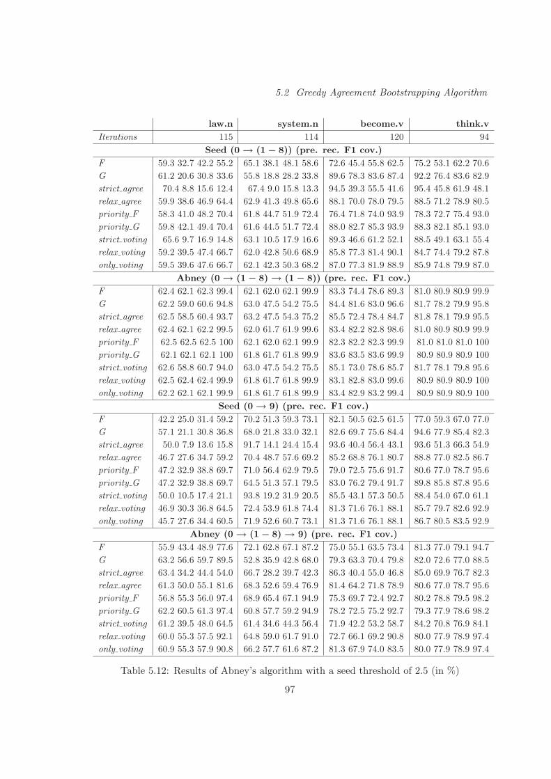
5.2 Greedy Agreement Bootstrapping Algorithm
law.n system.n become.v think.vIterations 115 114 120 94
Seed (0 → (1 − 8)) (pre. rec. F1 cov.)F 59.3 32.7 42.2 55.2 65.1 38.1 48.1 58.6 72.6 45.4 55.8 62.5 75.2 53.1 62.2 70.6G 61.2 20.6 30.8 33.6 55.8 18.8 28.2 33.8 89.6 78.3 83.6 87.4 92.2 76.4 83.6 82.9strict agree 70.4 8.8 15.6 12.4 67.4 9.0 15.8 13.3 94.5 39.3 55.5 41.6 95.4 45.8 61.9 48.1relax agree 59.9 38.6 46.9 64.4 62.9 41.3 49.8 65.6 88.1 70.0 78.0 79.5 88.5 71.2 78.9 80.5priority F 58.3 41.0 48.2 70.4 61.8 44.7 51.9 72.4 76.4 71.8 74.0 93.9 78.3 72.7 75.4 93.0priority G 59.8 42.1 49.4 70.4 61.6 44.5 51.7 72.4 88.0 82.7 85.3 93.9 88.3 82.1 85.1 93.0strict voting 65.6 9.7 16.9 14.8 63.1 10.5 17.9 16.6 89.3 46.6 61.2 52.1 88.5 49.1 63.1 55.4relax voting 59.2 39.5 47.4 66.7 62.0 42.8 50.6 68.9 85.8 77.3 81.4 90.1 84.7 74.4 79.2 87.8only voting 59.5 39.6 47.6 66.7 62.1 42.3 50.3 68.2 87.0 77.3 81.9 88.9 85.9 74.8 79.9 87.0
Abney (0 → (1 − 8) → (1 − 8)) (pre. rec. F1 cov.)F 62.4 62.1 62.3 99.4 62.1 62.0 62.1 99.9 83.3 74.4 78.6 89.3 81.0 80.9 80.9 99.9G 62.2 59.0 60.6 94.8 63.0 47.5 54.2 75.5 84.4 81.6 83.0 96.6 81.7 78.2 79.9 95.8strict agree 62.5 58.5 60.4 93.7 63.2 47.5 54.3 75.2 85.5 72.4 78.4 84.7 81.8 78.1 79.9 95.5relax agree 62.4 62.1 62.2 99.5 62.0 61.7 61.9 99.6 83.4 82.2 82.8 98.6 81.0 80.9 80.9 99.9priority F 62.5 62.5 62.5 100 62.1 62.0 62.1 99.9 82.3 82.2 82.3 99.9 81.0 81.0 81.0 100priority G 62.1 62.1 62.1 100 61.8 61.7 61.8 99.9 83.6 83.5 83.6 99.9 80.9 80.9 80.9 100strict voting 62.6 58.8 60.7 94.0 63.0 47.5 54.2 75.5 85.1 73.0 78.6 85.7 81.7 78.1 79.8 95.6relax voting 62.5 62.4 62.4 99.9 61.8 61.7 61.8 99.9 83.1 82.8 83.0 99.6 80.9 80.9 80.9 100only voting 62.2 62.1 62.1 99.9 61.8 61.7 61.8 99.9 83.4 82.9 83.2 99.4 80.9 80.9 80.9 100
Seed (0 → 9) (pre. rec. F1 cov.)F 42.2 25.0 31.4 59.2 70.2 51.3 59.3 73.1 82.1 50.5 62.5 61.5 77.0 59.3 67.0 77.0G 57.1 21.1 30.8 36.8 68.0 21.8 33.0 32.1 82.6 69.7 75.6 84.4 94.6 77.9 85.4 82.3strict agree 50.0 7.9 13.6 15.8 91.7 14.1 24.4 15.4 93.6 40.4 56.4 43.1 93.6 51.3 66.3 54.9relax agree 46.7 27.6 34.7 59.2 70.4 48.7 57.6 69.2 85.2 68.8 76.1 80.7 88.8 77.0 82.5 86.7priority F 47.2 32.9 38.8 69.7 71.0 56.4 62.9 79.5 79.0 72.5 75.6 91.7 80.6 77.0 78.7 95.6priority G 47.2 32.9 38.8 69.7 64.5 51.3 57.1 79.5 83.0 76.2 79.4 91.7 89.8 85.8 87.8 95.6strict voting 50.0 10.5 17.4 21.1 93.8 19.2 31.9 20.5 85.5 43.1 57.3 50.5 88.4 54.0 67.0 61.1relax voting 46.9 30.3 36.8 64.5 72.4 53.9 61.8 74.4 81.3 71.6 76.1 88.1 85.7 79.7 82.6 92.9only voting 45.7 27.6 34.4 60.5 71.9 52.6 60.7 73.1 81.3 71.6 76.1 88.1 86.7 80.5 83.5 92.9
Abney (0 → (1 − 8) → 9) (pre. rec. F1 cov.)F 55.9 43.4 48.9 77.6 72.1 62.8 67.1 87.2 75.0 55.1 63.5 73.4 81.3 77.0 79.1 94.7G 63.2 56.6 59.7 89.5 52.8 35.9 42.8 68.0 79.3 63.3 70.4 79.8 82.0 72.6 77.0 88.5strict agree 63.4 34.2 44.4 54.0 66.7 28.2 39.7 42.3 86.3 40.4 55.0 46.8 85.0 69.9 76.7 82.3relax agree 61.3 50.0 55.1 81.6 68.3 52.6 59.4 76.9 81.4 64.2 71.8 78.9 80.6 77.0 78.7 95.6priority F 56.8 55.3 56.0 97.4 68.9 65.4 67.1 94.9 75.3 69.7 72.4 92.7 80.2 78.8 79.5 98.2priority G 62.2 60.5 61.3 97.4 60.8 57.7 59.2 94.9 78.2 72.5 75.2 92.7 79.3 77.9 78.6 98.2strict voting 61.2 39.5 48.0 64.5 61.4 34.6 44.3 56.4 71.9 42.2 53.2 58.7 84.2 70.8 76.9 84.1relax voting 60.0 55.3 57.5 92.1 64.8 59.0 61.7 91.0 72.7 66.1 69.2 90.8 80.0 77.9 78.9 97.4only voting 60.9 55.3 57.9 90.8 66.2 57.7 61.6 87.2 81.3 67.9 74.0 83.5 80.0 77.9 78.9 97.4
Table 5.12: Results of Abney’s algorithm with a seed threshold of 2.5 (in %)
97

5 Bootstrapping
law.n system.n become.v think.vIterations 93 0 137 101
Seed (0 → (1 − 8)) (pre. rec. F1 cov.)F 56.1 48.5 52.1 86.5 63.5 54.9 58.9 86.4 69.0 58.9 63.5 85.4 71.7 63.9 67.6 89.2G 59.4 42.6 49.6 71.6 55.0 37.5 44.6 68.2 88.0 80.0 83.8 91.0 87.7 76.8 81.9 87.5strict agree 65.5 25.7 36.9 39.2 68.6 25.1 36.8 36.6 91.1 50.4 64.9 55.3 90.4 55.5 68.8 61.5relax agree 58.2 42.6 49.2 73.1 61.6 44.0 51.3 71.3 87.0 65.9 75.0 75.7 84.2 67.8 75.1 80.6priority F 55.5 53.3 54.4 96.0 61.3 58.0 59.6 94.6 71.2 70.0 70.6 98.4 71.9 70.4 71.2 97.9priority G 57.0 54.7 55.8 96.0 56.2 53.2 54.7 94.6 85.8 84.4 85.1 98.4 84.4 82.6 83.5 97.9strict voting 59.8 35.0 44.2 58.5 63.6 35.7 45.7 56.2 76.8 56.7 65.3 73.8 79.5 60.7 68.8 76.3relax voting 56.2 51.9 54.0 92.5 60.0 54.6 57.2 90.9 76.6 72.2 74.3 94.2 76.5 73.0 74.7 95.4only voting 57.8 51.5 54.4 89.1 60.0 52.8 56.2 87.9 82.4 75.8 79.0 91.9 80.1 74.4 77.2 92.9
Abney (0 → (1 − 8) → (1 − 8)) (pre. rec. F1 cov.)F 60.1 59.9 60.0 99.7 - 79.0 77.8 78.4 98.5 85.3 85.1 85.2 99.8G 61.7 47.8 53.9 77.4 - 83.2 79.1 81.1 95.0 87.8 84.5 86.1 96.2strict agree 62.7 45.0 52.4 71.7 - 83.7 73.9 78.5 88.3 88.1 82.2 85.1 93.3relax agree 60.6 57.3 58.9 94.6 - 82.0 77.8 79.8 94.9 87.1 84.6 85.8 97.1priority F 60.1 60.1 60.1 100 - 78.8 78.8 78.8 100 85.4 85.3 85.3 99.9priority G 59.9 59.9 59.9 100 - 81.8 81.8 81.8 100 86.8 86.7 86.8 99.9strict voting 61.9 47.6 53.8 77.0 - 81.7 75.7 78.6 92.6 87.1 83.4 85.2 95.8relax voting 60.0 59.9 60.0 99.9 - 80.2 79.5 79.9 99.1 86.1 85.7 85.9 99.6only voting 60.3 59.6 60.0 98.8 - 81.0 80.2 80.6 98.9 86.6 86.0 86.3 99.3
Seed (0 → 9) (pre. rec. F1 cov.)F 55.7 51.3 53.4 92.1 73.5 64.1 68.5 87.2 76.8 67.0 71.6 87.2 75.5 65.5 70.1 86.7G 71.2 48.7 57.8 68.4 63.0 43.6 51.5 69.2 82.1 71.6 76.5 87.2 91.8 79.7 85.3 86.7strict agree 77.8 27.6 40.8 35.5 79.3 29.5 43.0 37.2 88.9 51.4 65.1 57.8 93.9 54.9 69.3 58.4relax agree 64.2 44.7 52.7 69.7 76.4 53.9 63.2 70.5 84.6 70.6 76.9 83.5 89.4 74.3 81.2 83.2priority F 58.1 56.6 57.3 97.4 74.3 70.5 72.4 94.9 76.2 76.2 76.2 100 77.7 77.0 77.3 99.1priority G 62.2 60.5 61.3 97.4 64.9 61.5 63.2 94.9 81.7 81.7 81.7 100 88.4 87.6 88.0 99.1strict voting 66.0 40.8 50.4 61.8 72.3 43.6 54.4 60.3 83.1 58.7 68.8 70.6 82.7 59.3 69.1 71.7relax voting 60.3 57.9 59.1 96.1 72.6 68.0 70.2 93.6 81.0 78.0 79.4 96.3 81.7 78.8 80.2 96.5only voting 57.4 51.3 54.2 89.5 73.1 62.8 57.6 85.9 81.3 79.8 80.6 98.2 81.5 77.9 79.6 95.6
Abney (0 → (1 − 8) → 9) (pre. rec. F1 cov.)F 65.7 57.9 61.5 88.2 - 78.4 69.7 73.8 89.0 81.3 77.0 79.1 94.7G 75.4 56.6 64.7 75.0 - 81.0 74.3 77.5 91.7 89.0 78.8 83.6 88.5strict agree 81.8 35.5 49.6 43.4 - 85.1 57.8 68.9 67.9 93.3 62.0 74.5 66.4relax agree 78.4 52.6 63.0 67.1 - 84.2 73.4 78.4 87.2 92.6 77.0 84.1 83.2priority F 66.2 61.8 64.0 93.4 - 79.8 79.8 79.8 100 82.3 82.3 82.3 100priority G 74.7 69.7 72.1 93.4 - 79.8 79.8 79.8 100 88.5 88.5 88.5 100strict voting 62.3 43.4 51.2 69.7 - 82.6 65.1 72.8 78.9 81.9 68.1 74.4 83.2relax voting 64.8 60.5 62.6 93.4 - 82.2 80.7 81.5 98.2 83.2 83.2 83.2 100only voting 66.7 60.5 63.5 90.8 - 84.1 82.6 83.3 98.2 85.6 84.1 84.8 98.2
Table 5.13: Results of Abney’s algorithm with a seed threshold of 2 (in %)
98

5.2 Greedy Agreement Bootstrapping Algorithm
threshold 2.0 in both test sets.
In fact, for three words (law.n, become.v and think.v) the greedy agreement algorithmobtains better figures than the three baselines (MFC, Decision Lists and LazyBoostingtrained only using fold 0, see also tables 5.9 and 5.10). For instance, for noun law usingthreshold 3.0 and testing on fold 9 and using priority F and priority G achieves an F1measure of 64.8, while the LazyBoosting baseline obtains 64.5. The same also holds fortest on folds 1-8 and five combination rules achieving 60.4 instead of 59.8 F1 measure ofthe LazyBoosting baseline.
Regarding the best parameters for each word when testing on fold 9 (a new corpora notused during the bootstrapping), the best results for noun law are obtained when applyingpriority G combination rule and threshold 2.0 achieving an F1 measure of 72.1, whichrepresents an improvement of 7.6 points over the best baseline (LB). For the verb become,the best results are achieved when applying priority F combination rule and threshold 3.0obtaining the same figures than the best baseline (an F1 measure of 85.3 for LB). For theverb think.v, the best results are obtained when applying priority G combination rule andthreshold 2.0 achieving an F1 measure of 88.5, which represents an improvement of 1.8points over the best baseline (also LB).
However, for the noun system, none of the parameter combinations obtain betterperformance than the best baseline. The best results in this case are obtained whenusing threshold 3.0 and F and priority F rule combinations achieving an F1 measure of67.1, which is 7.6 points below the best baseline for this word (MFC). In fact, the othertwo Machine Learning algorithms (DL and LB) are not able to beat the MFC (with an F1measure of 74.7), which possibly denotes a biased sense distribution and a very difficulttask. It could be also the case that the whole set of features (and also possibly the twoviews) do not characterise appropriately the examples of this word.
It should be also noted that these results are obtained covering almost the whole fold9 (over 93% coverage).
Now, if we consider folds 1-8 for testing, only for the noun law the greedy agreementalgorithm obtains better F1 figures than the three baselines.
Regarding the best parameters for each word when testing on folds 1-8 (the samecorpora used for the bootstrapping), the best results for noun law are obtained whenapplying priority F combination rule and threshold 2.5 achieving an F1 measure of 62.5,which represents an improvement of 2.7 points over the best baseline (LB obtains an F1of 59.8). The best results for the noun system are obtained when using threshold 2.5 andF and priority F combination rules achieving an F1 measure of 62.1, which is 12.6 pointsbelow the best baseline for this word (again the MFC), but only 0.2 points below the best
99

5 Bootstrapping
Machine Learning algorithm (LB with an F1 of 62.3). For the verb become, the best resultsare achieved when applying priority G combination rule and threshold 3.0 achieving anF1 measure of 84.9, which is 2.3 points below the best baseline for this word (LB). Finally,for the verb think, the best results are achieved when applying priority G combinationrule and threshold 2.0 achieving an F1 measure of 86.8, which is 0.4 points below the bestbaseline for this word (LB).
Summarising, the threshold parameter affects directly the initial coverage andprecision. Obviously, the higher is the threshold, the higher the initial precision, and lowerthe initial coverage, which not surprisingly has a direct relationship with the behaviour ofthe bootstrapping algorithm. The best results are obtained using priority F or priority Gcombination rules. When performing the test on fold 9 (not seen by the bootstrappingalgorithm), three of the four words, the Abney’s algorithm is able to obtain betterperformances than the baselines. However, when using folds 1-8 for testing (those used bythe bootstrapping algorithm) only one word is able to outperform the baselines.
There are at least two points in which these experiments are different from thosepreviously reported for the Named Entity Recognition task (Collins and Singer, 1999).The first one is the amount of unlabelled examples used for the bootstrapping. Theexperiments on Named Entity Recognition used around 90,000 unlabelled examples (twoorders of magnitude higher than those reported here, which consist on about 500 unlabelledexamples). The second substantial difference is the high precision rates of the initial seeds.The Collins and Singer’s work report rules of almost 100% precision while we are reportingprecisions in the range of 60% to 90%.
Thus, our next steps on this research will consist on evaluating the performancesof non absolute thresholds. Instead, we plan to use relative thresholds associated toprecision, recall, coverage or F1 measures. We also plan to use a larger number ofunlabelled examples gathered from the British National Corpus. For instance, in BNCthere are 19,873 examples for the noun “law”, 40,478 examples for noun “system”, 53,844occurrences of the verb “become” and 86,564 examples for verb “think”. After this initialset of experiments, we also plan to use a more realistic evaluation scenario. We plan to useall the senses of the words (7 for law.n, 8 for system.n, 4 for become.v and 8 for think.v)and their whole set of labelled examples from the DSO (around 1,500) as a bootstrappingcorpora (750 examples) and as test corpora (750 examples).
100

5.3 Conclusions and Current/Further Work
5.3 Conclusions and Current/Further Work
The use of unlabelled data to train classifiers for Word Sense Disambiguation is a verychallenging line of research in order to develop a really robust, complete and accurateWord Sense Tagger (Agirre et al., 2005). Looking at the results of the experiments of thefirst section of this chapter, we can conclude that, at this moment, the use of unlabelledexamples with the transductive approach is not useful for Word Sense Disambiguation.At this point, there is a line of research to explore; to further study on the differencesand similarities between Text Categorisation and Word Sense Disambiguation models, inorder to develop a Word Sense Disambiguation model “compatible” with the transductiveapproach.
The second section of this chapter explores the application of the Greedy Agreementalgorithm of Abney (2002) to Word Sense Disambiguation. It consists of the previoususe of Decision Lists in order to obtain the seeds. The atomic rules of Decision Lists aresimilar to those of Abney’s algorithm. We have applied it to only 2 senses of 4 wordsof the DSO corpus in order to deal with a big amount of examples per sense. Then wehave compared the results to a naive Most Frequent Classifier, Decision Lists and LazyBoosting, and obtained comparable or higher results (in accuracy). This approximationseems to be useful in order to apply bootstrapping to the Word Sense Disambiguationdata.
Since the bootstrapping algorithm on this setting is providing interesting but notconclusive results, we plan to continue the study of the behaviour of this approach on amore realistic scenario. It should consist of:
• testing the framework with all word senses (not only with 2 of them),
• increasing the feature sets of the views with those described in appendix B1,
• optimising the threshold see extraction for each word by applying cross-validation,
• and finally, testing the Greedy Agreement algorithm using large sets of unlabelleddata extracted from the British National Corpus; enlarging both the training setand the set used for the extraction of the seed rules.
1One of the difficulties when applying the greedy agreement algorithm is the use of a limited number of
features in the views. So, the results of the views are far below than when using the complete feature set.
101

5 Bootstrapping
102

Chapter 6
Evaluation in Senseval Exercises
This chapter is devoted to explain our participation in the international evaluations onWord Sense Disambiguation. Concretely, we have participated in the English LexicalSample task of both Senseval-2 (Kilgarriff, 2001) and Senseval-3 (Mihalcea et al., 2004)events. We start this chapter with a description of the English Lexical Sample task data forboth Senseval-2 and Senseval-3. Section 6.2 explains the system presented at Senseval-2and section 6.3 shows the results of a comparative study of the best six methods onSenseval-2 English Lexical Sample task. Section 6.4 is devoted to present the architectureof the system presented at Senseval-3 and section 6.3.2 shows further experiments onfeatures with the system.
6.1 Senseval Corpora
This section explains in detail the Senseval English Lexical Sample data1. Senseval-2corpus consists of 8,611 training and 4,328 test examples of 73 words. These exampleswere extracted from the British National Corpus2. Figure 6.1 shows an example fromthe Senseval-2 corpus. It corresponds to the instance art.40012, which has been labelledwith two senses: P and arts%1:09:00::. Most of the examples have only a sense but thereare exceptions with two or three senses. The word to be disambiguated is marked by the<head> label and is always located in the last sentence of the context. The Senseval-2 senseinventory is a prerelease of WordNet 1.7. Table 6.1 shows the noun art in that inventory.For each word the corpus has some extra “sense labels”: label P for proper-names; andlabel U for unassignable. Unassignable stands for examples in which human annotators
1http://www.senseval.org2http://www.natcorp.ox.ac.uk
103

6 Evaluation in Senseval Exercises
had problems in labelling. Nouns and adjectives can be also monosemous multiwords–such as art class%1:04:00:: or art collection%1:14:00:: for the word art–; and verbs canbe polysemous phrasal verbs –such as work on%2:41:00:: for the verb work. Phrasal verbshave been tagged. So, they should be treated as independent words (see figure 6.2 for anexample). Senseval providers referred to the sense labels of the examples as keys and thelabels provided by the participants as system votes.
sense word pos descriptorart%1:04:00:: art noun creationart%1:06:00:: art noun artworksart%1:09:00:: art noun skillart%1:10:00:: art noun inabook
Table 6.1: Sense Inventory for the noun art in Senseval-2 corpus
Senseval-3 corpus consists of 7,860 training and 3,944 test examples of 57 words. Nounsand adjectives of Senseval-3 data have been annotated using the WordNet 1.7.1 senseinventory, and verbs with labels based on Wordsmyth definitions3 (see appendix C forWeb references to both resources). Senseval-3 sense inventory has neither multiwords, norphrasal verbs, nor proper-nouns. That is, the senses used are only the senses like those oftable 6.1 and the unassignable U label. This corpus has a large number of examples withmore than one sense assigned. Figure 6.3 shows and example from Senseval-3 corpus.
6.2 TALP System at Senseval-2
This section describes the architecture and results of the TALP system presented at theSenseval-2 exercise for the English Lexical Sample task. The system was developed onthe basis of LazyBoosting (Escudero et al., 2000c), the boosting-based approach for WordSense Disambiguation explained in section 3.4. In order to better fit the Senseval-2 domain,some improvements were made, including: (1) features that take into account domaininformation, (2) an specific treatment of multiwords, and (3) a hierarchical decompositionof the multiclass classification problem, similar to that of Yarowsky (2000). All theseissues will be briefly described in the following sections.
3A mapping between Wordsmyth and WordNet verb senses was provided.
104
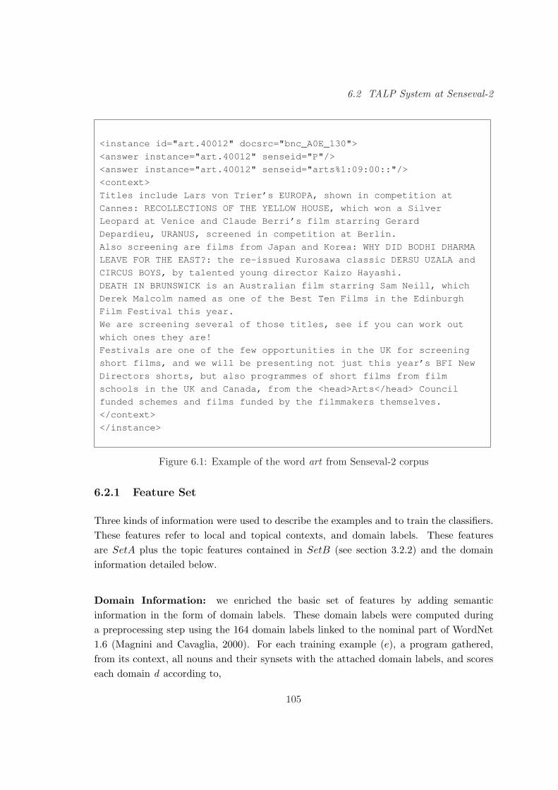
6.2 TALP System at Senseval-2
<instance id="art.40012" docsrc="bnc_A0E_130">
<answer instance="art.40012" senseid="P"/>
<answer instance="art.40012" senseid="arts%1:09:00::"/>
<context>
Titles include Lars von Trier’s EUROPA, shown in competition at
Cannes: RECOLLECTIONS OF THE YELLOW HOUSE, which won a Silver
Leopard at Venice and Claude Berri’s film starring Gerard
Depardieu, URANUS, screened in competition at Berlin.
Also screening are films from Japan and Korea: WHY DID BODHI DHARMA
LEAVE FOR THE EAST?: the re-issued Kurosawa classic DERSU UZALA and
CIRCUS BOYS, by talented young director Kaizo Hayashi.
DEATH IN BRUNSWICK is an Australian film starring Sam Neill, which
Derek Malcolm named as one of the Best Ten Films in the Edinburgh
Film Festival this year.
We are screening several of those titles, see if you can work out
which ones they are!
Festivals are one of the few opportunities in the UK for screening
short films, and we will be presenting not just this year’s BFI New
Directors shorts, but also programmes of short films from film
schools in the UK and Canada, from the <head>Arts</head> Council
funded schemes and films funded by the filmmakers themselves.
</context>
</instance>
Figure 6.1: Example of the word art from Senseval-2 corpus
6.2.1 Feature Set
Three kinds of information were used to describe the examples and to train the classifiers.These features refer to local and topical contexts, and domain labels. These featuresare SetA plus the topic features contained in SetB (see section 3.2.2) and the domaininformation detailed below.
Domain Information: we enriched the basic set of features by adding semanticinformation in the form of domain labels. These domain labels were computed duringa preprocessing step using the 164 domain labels linked to the nominal part of WordNet1.6 (Magnini and Cavaglia, 2000). For each training example (e), a program gathered,from its context, all nouns and their synsets with the attached domain labels, and scoreseach domain d according to,
105

6 Evaluation in Senseval Exercises
<instance id="work.097">
<answer instance="work.097" senseid="work_on%2:41:00::"/>
<context>
How could anyone know what to do with an assortment like that ? ?
Perhaps he had better have someone help him put up the pegboard and
build the workbench - someone who knew what he was about .
Then at least he would have a place to hang his tools and something
to <head sats="work_on.097:0">work</head>
<sat id="work_on.097:0">on</sat> .
</context>
</instance>
Figure 6.2: Example of phrasal verb work on from Senseval-2 corpus
<instance id="argument.n.bnc.00066601" docsrc="BNC">
<answer instance="argument.n.bnc.00066601"
senseid="argument%1:09:00::"/>
<answer instance="argument.n.bnc.00066601"
senseid="argument%1:10:02::"/>
<answer instance="argument.n.bnc.00066601" senseid="U"/>
<context>
The whole system was ill - conceived from the outset . That some very
large companies should have lost a great deal of money on their
little experiment shows only how unwise their decision to pursue the
technology was . Look at the <head>arguments</head> . Since calls
must be made close to a node , then why not simply find a
telephone kiosk must work these days and the cost will only be at
the standard rate . Then there is the absurd lack of ability to
receive calls .
</context>
</instance>
Figure 6.3: Example of noun argument from Senseval-3 corpus
106

6.2 TALP System at Senseval-2
Weight(d) =ContextDomains(d)DomainFreqWN(d)
· LabelsDomain
where LabelsDomain is the ratio of the total number of labelled WordNet synsets over thetotal number of domain labels; DomainFreqWN(d) is the frequency of the domain d onWordNet; and ContextDomains(d) is,
ContextDomains(d) =∑
w∈nouns(e)
WordDomains(w, d)SumWeights(w)
where
WordDomains(w, d) =∑
{s∈Synsets(w)|s∈d}
(1− Position(w, s)− 1
|Synsets(w)|)
and
SumWeights(w) =∑
s∈Synsets(w)
|Domains(s)| ·(
1− Position(w, s)− 1|Synsets(w)|
)
where Position(w,s) is the frequency position relative to WordNet of the synset s in theword w (e.g., 2 stands for the second most frequent sense of the word); |Synsets(w)| standsfor the number of synsets of the word w ; and |Domains(s)| is referred to the number ofdomains to which synset s is connected.
This function assigns to each example a set of domains labels depending on the numberof domain labels assigned to each noun and their relative frequencies in the whole WordNet.Each domain label of the example is ranked by a weight, and the list of domains is prunedby a threshold. That is, the result of this procedure is the set of domain labels thatachieve a score higher than a threshold of 0.04, which are incorporated as regular featuresfor describing the example. Figure 6.4 shows a text example and the domains extractedapplying the algorithms with their corresponding weights4. We used this information tobuilt a bag of domains.
4The example has been applied using not only nouns, but also verbs, adjectives and adverbs. At
Senseval-2 time, there were available domains for nouns only.
107

6 Evaluation in Senseval Exercises
ExampleA new art fair will take place at theG-Mex Centre , Manchester from 18 to 21March . Paintings , drawings and sculpturefrom every period of art during the last 350years will be on display ranging from a Tudorportrait to contemporary British art .
domain weightpainting 7.07art 6.79time period 1.64anthropology 1.39sociology 1.21quality 0.25factotum 0.16
Figure 6.4: Text example with its corresponding domains
6.2.2 Preprocessing and Hierarchical Decomposition
As an initial experiment we selected a representative sample, containing the most frequentwords of the Senseval-2 training data, and applied the LazyBoosting system (see section3.4) straightforwardly on this sample. The results achieved after a 10-fold cross-validationprocedure were extremely bad, mainly due to the fact that most of the words containtoo many senses and too few examples per sense to induce reliable classifiers. With theaim of improving the performance of the learning algorithm, two different simplificationswere carried out. Firstly, training examples consisting of a multiword have been processedseparately. During training, multiwords have been saved into a separate file. At test time,all examples found in this multiword file are automatically tagged as multiwords. As anexample, the word bar appears in the training set with 22 labels. But only the 10 sensesshowed in the left table of figure 6.5 are single words. The remaining 12 are multiwordswhich are considered unambiguous. In the official competition, labels ‘U’ and ‘P’ werecompletely ignored by our system. Thus, the examples labelled with these classes have notbeen considered during the training, and no test examples have been tagged with them.
Secondly, we have reduced the sense granularity, by hierarchically decomposing thelearning process into two steps, following the work of Yarowsky (2000). At the firstlevel, the learning algorithm was trained to classify among the labels corresponding tothe WordNet semantic files, and, additionally, the semantic file labels with less than 10training examples were automatically discarded. If less than two senses remain, no trainingis performed and the Most-frequent-sense Classifier is applied at testing time. As anexample, for the word ‘bar’, in this first step the system is trained to classify betweenthe labels of the top-right table of figure 6.55. Note that senses bar%1:04, bar%1:23 andbar%1:17 have been discarded out because there are not enough training examples. At thesecond level, one classifier is trained for each of the resulting semantic-file labels of the first
5Numbers 06, 14, 10, 04, 23, and 17 correspond to the WordNet Lexicographical Files.
108
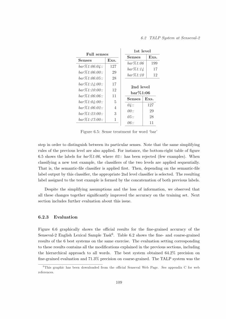
6.2 TALP System at Senseval-2
Full sensesSenses Exs.bar%1:06:04:: 127bar%1:06:00:: 29bar%1:06:05:: 28bar%1:14:00:: 17bar%1:10:00:: 12bar%1:06:06:: 11bar%1:04:00:: 5bar%1:06:02:: 4bar%1:23:00:: 3bar%1:17:00:: 1
1st levelSenses Exs.bar%1:06 199bar%1:14 17bar%1:10 12
2nd levelbar%1:06
Senses Exs.04:: 12700:: 2905:: 2806:: 11
Figure 6.5: Sense treatment for word ‘bar’
step in order to distinguish between its particular senses. Note that the same simplifyingrules of the previous level are also applied. For instance, the bottom-right table of figure6.5 shows the labels for bar%1:06, where 02:: has been rejected (few examples). Whenclassifying a new test example, the classifiers of the two levels are applied sequentially.That is, the semantic-file classifier is applied first. Then, depending on the semantic-filelabel output by this classifier, the appropriate 2nd level classifier is selected. The resultinglabel assigned to the test example is formed by the concatenation of both previous labels.
Despite the simplifying assumptions and the loss of information, we observed thatall these changes together significantly improved the accuracy on the training set. Nextsection includes further evaluation about this issue.
6.2.3 Evaluation
Figure 6.6 graphically shows the official results for the fine-grained accuracy of theSenseval-2 English Lexical Sample Task6. Table 6.2 shows the fine- and coarse-grainedresults of the 6 best systems on the same exercise. The evaluation setting correspondingto these results contains all the modifications explained in the previous sections, includingthe hierarchical approach to all words. The best system obtained 64.2% precision onfine-grained evaluation and 71.3% precision on coarse-grained. The TALP system was the
6This graphic has been downloaded from the official Senseval Web Page. See appendix C for web
references.
109

6 Evaluation in Senseval Exercises
sixth of 21 supervised systems and the difference from the first was of only 4.8% and 4.2%in fine-grained and coarse-grained precision, respectively.
Figure 6.6: Senseval-2 Results
After the Senseval-2 event, we added a very simple Named-entity Recogniser to thepart-of-speech tagger that was not finished at the time of the event, but the systemcontinued completely ignoring the ‘U’ label. We also evaluated which parts of the systemcontributed most to the improvement in performance. Figure 6.7 shows the accuracyresults of the four combinations resulting from using (or not) domain-label featuresand hierarchical decomposition. These results have been calculated over the test set ofSenseval-2.
On the one hand, it becomes clear that enriching the feature set with domain labelssystematically improves the results in all cases, and that this difference is especiallynoticeable in the case of nouns (over 3 points of improvement). On the other hand,the use of the hierarchies is unexpectedly useless in all cases. Although it is productivein some particular words (3 nouns, 12 verbs and 5 adjectives) the overall performance issignificantly lower. A fact that can explain this situation is that the first-level classifiersdo not succeed at classifying semantic-file labels with high precision levels (the averageaccuracy of first-level classifiers is only slightly over 71%) and that this important error is
110
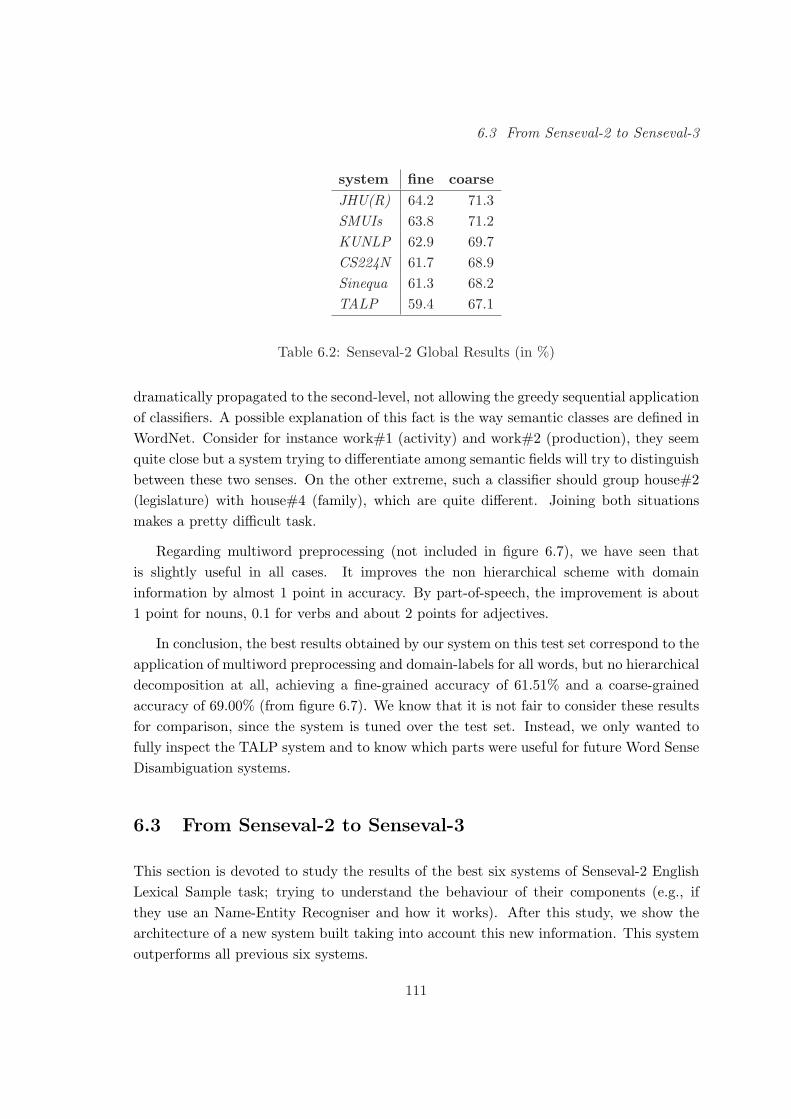
6.3 From Senseval-2 to Senseval-3
system fine coarseJHU(R) 64.2 71.3SMUIs 63.8 71.2KUNLP 62.9 69.7CS224N 61.7 68.9Sinequa 61.3 68.2TALP 59.4 67.1
Table 6.2: Senseval-2 Global Results (in %)
dramatically propagated to the second-level, not allowing the greedy sequential applicationof classifiers. A possible explanation of this fact is the way semantic classes are defined inWordNet. Consider for instance work#1 (activity) and work#2 (production), they seemquite close but a system trying to differentiate among semantic fields will try to distinguishbetween these two senses. On the other extreme, such a classifier should group house#2(legislature) with house#4 (family), which are quite different. Joining both situationsmakes a pretty difficult task.
Regarding multiword preprocessing (not included in figure 6.7), we have seen thatis slightly useful in all cases. It improves the non hierarchical scheme with domaininformation by almost 1 point in accuracy. By part-of-speech, the improvement is about1 point for nouns, 0.1 for verbs and about 2 points for adjectives.
In conclusion, the best results obtained by our system on this test set correspond to theapplication of multiword preprocessing and domain-labels for all words, but no hierarchicaldecomposition at all, achieving a fine-grained accuracy of 61.51% and a coarse-grainedaccuracy of 69.00% (from figure 6.7). We know that it is not fair to consider these resultsfor comparison, since the system is tuned over the test set. Instead, we only wanted tofully inspect the TALP system and to know which parts were useful for future Word SenseDisambiguation systems.
6.3 From Senseval-2 to Senseval-3
This section is devoted to study the results of the best six systems of Senseval-2 EnglishLexical Sample task; trying to understand the behaviour of their components (e.g., ifthey use an Name-Entity Recogniser and how it works). After this study, we show thearchitecture of a new system built taking into account this new information. This systemoutperforms all previous six systems.
111

6 Evaluation in Senseval Exercises
nounsno dom. with dom.
fine coar. fine coar.no hier. 64.3 72.4 67.9 75.6hier. 63.0 71.1 64.3 71.5
verbsno dom. with dom.
fine coar. fine coar.no hier. 51.6 61.6 52.1 62.6hier. 50.3 60.8 51.1 62.0
adjectivesno dom. with dom.
fine coar. fine coar.no hier. 66.2 66.2 68.9 68.9hier. 65.4 65.4 68.2 68.2
Figure 6.7: Fine/coarse-grained evaluation (in %) for different settings and part-of-speech
6.3.1 System Decomposition
The Senseval-2 sense labels could be classified in different groups. These groups of labelscould be tackled with different modules.
Table 6.3 shows the overall results of the six best systems of Senseval-2: jhu(r)(Yarowsky et al., 2001), smuis (Mihalcea and Moldovan, 2001), kunlp (Seo et al., 2001),cs224n (Ilhan et al., 2001), sinequa (Crestan et al., 2001) and talp (Escudero et al.,2001). The columns stands, respectively, for the fine-grained accuracy, the number ofcorrect labelled examples in the test sample (in fine-grained evaluation), the coarse-grainedaccuracy and the number of examples correctly classified. There are 4,328 test examplesin the corpus. All examples were treated by all systems (coverage = 100%). So, precisionand recall are the same. Throughout all this study we have used the scorer of Senseval-27.A difference of only 5 points in fine-grained and of 4 points in coarse-grained accuracy canbe observed between the first and the last system.
Table 6.4 shows the agreement and kappa values between every pair of systems. Cellsabove the diagonal are the agreement between every pair of systems and those below thediagonal contain the kappa values. The maximum difference between pairs of systemsis of 8% of agreement (from 0.60 to 0.68). The low agreements (65%) of all pairs show
7Available at the web site (see appendix C).
112

6.3 From Senseval-2 to Senseval-3
system fine ok coarse okJHU(R) 64.2 2,780 71.3 3,086SMUIs 63.8 2,763 71.2 3,080KUNLP 62.9 2,724 69.7 3,016CS224N 61.7 2,670 68.9 2,981Sinequa 61.3 2,653 68.2 2,953TALP 59.4 2,571 67.1 2,903
Table 6.3: Senseval-2 Global Results (in %)
the big differences in the outputs of the systems. The kappa values differ more thansimple agreement (from 0.22 to 0.35). This measure shows evidence of a large differencein performance among some of the systems.
jhu smuis kunlp cs224n sinequa talpjhu - 0.62 0.67 0.65 0.64 0.61smui 0.34 - 0.66 0.60 0.64 0.60kunlp 0.35 0.34 - 0.68 0.67 0.64cs224n 0.29 0.22 0.31 - 0.67 0.65sinequa 0.28 0.31 0.31 0.25 - 0.64talp 0.27 0.27 0.30 0.25 0.26 -
Table 6.4: Agreement (above diagonal) and kappa (below diagonal) values between everypair of systems
Now we try to decompose the systems output (outcomes) in order to understand theirresults and the source of the differences among them. First, we clustered the test examplesas follows: P stands for Proper-names, mw for Multiwords, pv for Phrasal Verbs, U forUnassignable and ml for the set of examples with regular senses (e.g., sense bar%1:06:04::of the noun bar).
Table 6.5 shows the performance of the six systems taking into account only the Plabel. To do that, all files (both keys and system votes) were pruned, and only P labelsremained for testing. There are 146 P test examples in the corpus. This table shows,respectively, precision (pr), recall (rc), F1, number of correct labelled examples (ok), andnumber of examples attempted (att). Both fine-grained and coarse-grained results arethe same, due to the fact that label P has no hierarchy. Two of these systems (kunlpand talp) had no Name-Entity Recogniser. Two of them detected proper nouns with highprecision but a very poor recall, Sinequa and CS2224N (probably they tackled proper
113

6 Evaluation in Senseval Exercises
nouns as another label of the learning problem). And finally, the two best systems had acomponent to preprocess proper nouns. SMUIs had the best .
system pr rc F1 ok attJHU(R) 54.8 34.9 42.6 51 93SMUIs 81.6 48.6 60.9 71 87KUNLP N/A 0 N/A 0 0CS224N 66.7 1.4 2.7 2 3Sinequa 88.9 5.5 10.4 8 9TALP N/A 0 N/A 0 0
Table 6.5: Senseval-2 results on Proper-Names (in %)
Table 6.6 shows multiword treatment and has the same format of table 6.5. Thereare 170 multiword test examples in the corpus. Multiwords appeared only for nouns andadjectives, but not for verbs. In this group there is again a significant difference betweenthe two best system and the rest. They had the best multiword processor.
system pr rc F1 ok attJHU(R) 85.8 74.7 79.9 127 148SMUIs 88.8 68.0 77.0 151 222KUNLP 53.9 48.8 51.2 83 154CS224N 78.4 34.1 47.5 58 74Sinequa 90.3 54.7 68.1 93 103TALP 89.3 64.1 74.6 109 122
Table 6.6: Senseval-2 results on Multiwords (in %)
Table 6.7 has the same format as the previous two. It shows the results on the set ofphrasal verbs. There are 182 phrasal verbs test examples in the corpus. Phrasal verb labelswere in a hierarchy. For this reason this table contains fine-grained and coarse-grainedresults. Again, there are big differences. They ranged from 43.0% to 66.5% on precisionand from 26.9% to 65.4% of recall.
Next, table 6.8 shows the behaviour on the U -labelled examples. This label has nohierarchy. Only 3 systems treated this label, and they achieved very low recall results.There are 160 U test examples in the corpus.
Finally, the results on the core ml set of examples are shown in table 6.9. Thereare 3.733 ml test examples in the corpus. The results for nouns (1,412 examples), verbs
114

6.3 From Senseval-2 to Senseval-3
fine coarsesystem pr rc F1 ok pr rc F1 ok attJHU(R) 66.5 65.4 66.0 119 71.5 70.3 70.9 128 179SMUIs 58.0 57.7 57.9 105 65.7 65.4 65.6 119 181KUNLP 49.8 58.8 53.9 107 53.5 63.2 58.0 115 215CS224N 43.0 26.9 33.1 49 50.9 31.9 39.2 58 114Sinequa 59.5 42.9 49.9 78 65.6 47.3 55.0 86 131TALP 45.5 39.0 42.0 71 55.1 47.3 50.9 86 156
Table 6.7: Senseval-2 results on Phrasal Verbs (in %)
system pr rc F1 ok attJHU(R) 70.4 23.7 35.5 38 54SMUIs N/A 0 N/A 0 0KUNLP N/A 0 N/A 0 0CS224N 55.8 15.0 23.6 24 43Sinequa 61.5 10.0 17.2 16 26TALP N/A 0 N/A 0 0
Table 6.8: Senseval-2 results on the U label examples (in %)
(1,630 examples), and adjectives (691 examples) are presented by tables 6.10, 6.11 and6.12, respectively.
From these results, the first system in the competition, JHU(R), is not the bestsystem (from the machine learning perspective) for nouns and verbs -and nouns and verbsrepresented more than the half part of the test set. The main reason for obtaining thebest results resides in performing a better preprocessing of examples and treatment ofU, phrasal verbs, multiwords and proper-nouns cases. That is, it treated better than therest multiword, phrasal verbs, proper-nouns and the U label; maintaining a competitiveperformance on the ml set. There are no overall ml significant differences. SMUIs andKUNLP are better in verbs, and SMUIs in nouns; but JHU(R) is extremely good withadjectives.
The interaction between all components of the systems makes difficult to compare theMachine Learning algorithms. For this reason, we have extracted the intersection set ofall the examples in which every system have output a regular sense. This set has 3,520examples. The results are shown in table 6.13. Here, we can see that the four best systemshave very similar performance being KUNLP slightly better than the rest.
115
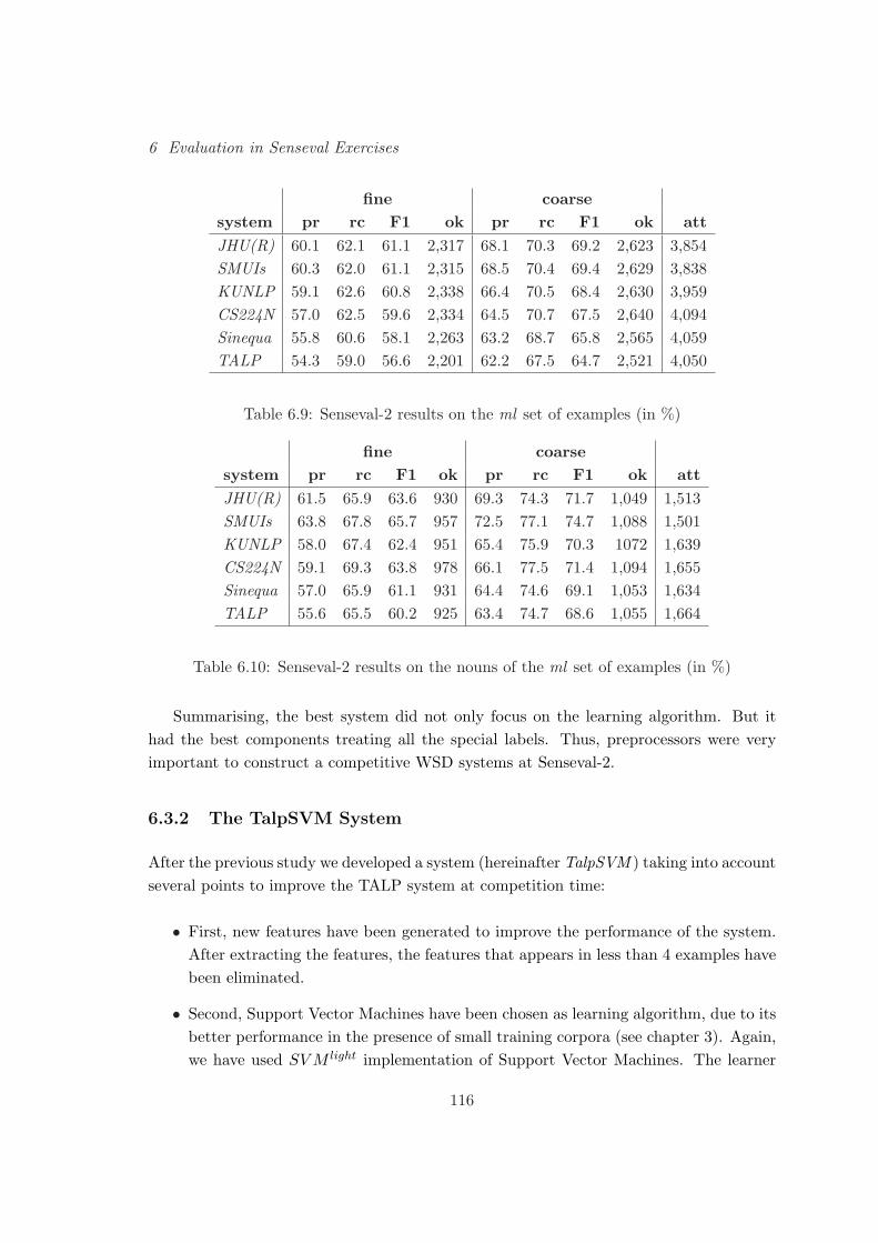
6 Evaluation in Senseval Exercises
fine coarsesystem pr rc F1 ok pr rc F1 ok attJHU(R) 60.1 62.1 61.1 2,317 68.1 70.3 69.2 2,623 3,854SMUIs 60.3 62.0 61.1 2,315 68.5 70.4 69.4 2,629 3,838KUNLP 59.1 62.6 60.8 2,338 66.4 70.5 68.4 2,630 3,959CS224N 57.0 62.5 59.6 2,334 64.5 70.7 67.5 2,640 4,094Sinequa 55.8 60.6 58.1 2,263 63.2 68.7 65.8 2,565 4,059TALP 54.3 59.0 56.6 2,201 62.2 67.5 64.7 2,521 4,050
Table 6.9: Senseval-2 results on the ml set of examples (in %)
fine coarsesystem pr rc F1 ok pr rc F1 ok attJHU(R) 61.5 65.9 63.6 930 69.3 74.3 71.7 1,049 1,513SMUIs 63.8 67.8 65.7 957 72.5 77.1 74.7 1,088 1,501KUNLP 58.0 67.4 62.4 951 65.4 75.9 70.3 1072 1,639CS224N 59.1 69.3 63.8 978 66.1 77.5 71.4 1,094 1,655Sinequa 57.0 65.9 61.1 931 64.4 74.6 69.1 1,053 1,634TALP 55.6 65.5 60.2 925 63.4 74.7 68.6 1,055 1,664
Table 6.10: Senseval-2 results on the nouns of the ml set of examples (in %)
Summarising, the best system did not only focus on the learning algorithm. But ithad the best components treating all the special labels. Thus, preprocessors were veryimportant to construct a competitive WSD systems at Senseval-2.
6.3.2 The TalpSVM System
After the previous study we developed a system (hereinafter TalpSVM ) taking into accountseveral points to improve the TALP system at competition time:
• First, new features have been generated to improve the performance of the system.After extracting the features, the features that appears in less than 4 examples havebeen eliminated.
• Second, Support Vector Machines have been chosen as learning algorithm, due to itsbetter performance in the presence of small training corpora (see chapter 3). Again,we have used SV M light implementation of Support Vector Machines. The learner
116

6.3 From Senseval-2 to Senseval-3
fine coarsesystem pr rc F1 ok pr rc F1 ok attJHU(R) 54.9 54.8 54.9 894 66.4 66.3 66.4 1,081 1,627SMUIs 55.5 55.3 55.4 902 66.8 66.6 66.7 1,085 1,625KUNLP 58.3 56.9 57.6 927 69.0 67.4 68.2 1,098 1,591CS224N 52.4 54.4 53.4 887 63.7 66.1 64.9 1,077 1,692Sinequa 52.4 53.9 53.1 878 63.2 64.9 64.0 1,058 1,675TALP 51.4 52.0 51.7 848 62.9 63.7 63.3 1,038 1,650
Table 6.11: Senseval-2 results on the verbs of the ml set of examples (in %)
fine coarsesystem pr rc F1 ok pr rc F1 ok attJHU(R) 69.0 71.3 70.1 493 69.0 71.3 70.1 493 714SMUIs 64.0 66.0 65.0 456 64.0 66.0 65.0 456 712KUNLP 63.1 66.6 64.8 460 63.1 66.6 64.8 460 729CS224N 62.8 67.9 65.3 469 62.8 67.9 65.3 469 747Sinequa 60.5 65.7 63.0 454 60.5 65.7 63.0 454 750TALP 58.2 61.9 60.0 428 58.2 61.9 60.0 428 736
Table 6.12: Senseval-2 results on the adjectives of the ml set of examples (in %)
takes as input all the examples of the training set that are not tagged as P, U,multiword neither phrasal verb, and label U has not been considered in the trainingstep neither in the test step.
• Third, the addition of new examples from other corpora have been tried tocompensate for the small number of examples of Senseval-2 corpora.
• And finally, we have tried to improve all preprocessing components.
Each example is labelled with 3 linguistic processors8: the FreeLing Part-of-Speechtagger (Atserias et al., 2006), from which the system extracts the lemmas of the words andthe Part-of-Speech tag; the Minipar parser (Lin, 1998), from which the syntactical relationsare extracted as features for the learners; and, finally, the TnT tagger (Brants, 1997), fromwhich the system extract the P tag (it is the target word tagged as Named-Entity by thetagger).
8See appendix C for web references of these 3 linguistics processors.
117
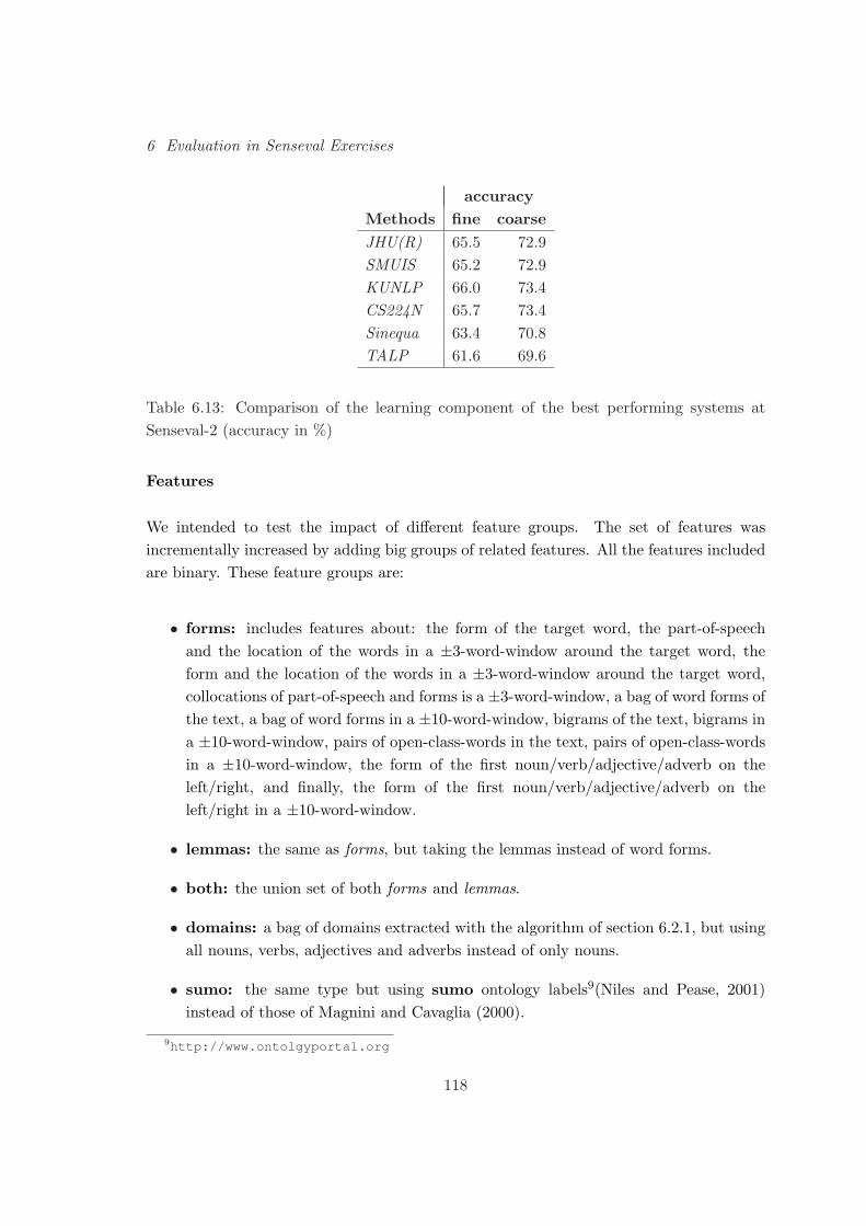
6 Evaluation in Senseval Exercises
accuracyMethods fine coarseJHU(R) 65.5 72.9SMUIS 65.2 72.9KUNLP 66.0 73.4CS224N 65.7 73.4Sinequa 63.4 70.8TALP 61.6 69.6
Table 6.13: Comparison of the learning component of the best performing systems atSenseval-2 (accuracy in %)
Features
We intended to test the impact of different feature groups. The set of features wasincrementally increased by adding big groups of related features. All the features includedare binary. These feature groups are:
• forms: includes features about: the form of the target word, the part-of-speechand the location of the words in a ±3-word-window around the target word, theform and the location of the words in a ±3-word-window around the target word,collocations of part-of-speech and forms is a ±3-word-window, a bag of word forms ofthe text, a bag of word forms in a ±10-word-window, bigrams of the text, bigrams ina ±10-word-window, pairs of open-class-words in the text, pairs of open-class-wordsin a ±10-word-window, the form of the first noun/verb/adjective/adverb on theleft/right, and finally, the form of the first noun/verb/adjective/adverb on theleft/right in a ±10-word-window.
• lemmas: the same as forms, but taking the lemmas instead of word forms.
• both: the union set of both forms and lemmas.
• domains: a bag of domains extracted with the algorithm of section 6.2.1, but usingall nouns, verbs, adjectives and adverbs instead of only nouns.
• sumo: the same type but using sumo ontology labels9(Niles and Pease, 2001)instead of those of Magnini and Cavaglia (2000).
9http://www.ontolgyportal.org
118

6.3 From Senseval-2 to Senseval-3
• minipar: a bag of syntactical relations extracted from the Minipar parser. Weconsidered also a feature that only has the syntactical relations of the target word.
Table 6.14 shows the result of the system using the different sets of features. As wecan see, all features sets seems to improve the performance of the system.
system fine coarseforms 62.6 69.7lemmas 63.9 70.5both 63.8 70.5both+sumo 63.8 70.7both+domains 64.3 71.0both+minipar 63.7 70.7both+all 64.6 71.2
Table 6.14: TalpSVM results using different feature sets (in %)
New Examples
Table 6.16 shows the effect of the addition of training examples from other corpora. wnestands for the examples in WordNet glosses; wng for the definitions in WordNet glosses;sc stands for sentences in the Semcor corpus10; and se2 represents the original Senseval-2English Lexical Sample task corpus. Table 6.15 shows the amount of examples extractedfrom each of these corpora.
source acr. number of examplesWN Examples wne 549WN Glosses wng 3,115Semcor sc 7,193
Table 6.15: Number of examples extracted from other corpora
Surprisingly, the addition of examples from other sources implies a decrease in accuracyresults (see table 6.16). This could be caused by the difference in the format of theexamples in the corpora.
10See appendix C for Web references.
119

6 Evaluation in Senseval Exercises
system fine coarsese2 63.6 70.5se2+wne 63.4 70.3se2+wng 62.3 69.5se2+sc 62.4 70.2all 62.0 70.0
Table 6.16: TalpSVM results adding different example sets (accuracy in %)
Preprocess
Table 6.17 shows the results of the proper-name component. Every row representsrespectively: the use of the P label, the use of the ml corresponding label, and the use ofboth labels for each example. The best option corresponds to ml that shows the lack ofutility of the component and evincing that a better Name-Entity Recogniser is needed.
system fine coarseP 64.6 71.2ml 64.8 71.7P+ml 64.7 71.4
Table 6.17: TalpSVM results using a Name-Entity Recogniser (accuracy in %)
The multiword component takes the information provided by Senseval-2 organisers(a list of the multiwords of appearing in the corpus plus its corresponding sense). Thismultiword list have been indexed and compared with the test examples in order to detectthem. Table 6.18 shows the behaviour of this component. mw stands for the use ofmultiwords component labels and ml for the Machine Learning classifier. The use of thiscomponent increases the fine-grained accuracy in 3.6% (from 61.6 to 64.8). The last rowrepresents the vote of both the multiword and that of the classifier.
system fine coarsemw 64.8 71.7ml 61.6 68.6mw+ml 63.2 70.2
Table 6.18: TalpSVM and multiword (in %)
Phrasal verbs have been tagged with the most frequent sense of the training set; or,
120

6.4 Senseval-3
if they did not appear in training set, with the most frequent sense of WordNet. Thebehaviour of the system including this component is shown in table 6.19. An increase of2% in accuracy is observed when using the phrasal verbs component.
system fine coarsepv 64.8 71.7ml 62.7 69.3pv+ml 63.2 69.8
Table 6.19: TalpSVM and phrasal verbs (in %)
6.3.3 Global Results
After the development, TalpSVM has been compared with the six best systems ofSenseval-2 competition. Tables 6.20 and 6.21 contain the results of the system to becompared with those in tables from 6.3 to 6.13. P stands for the use of P label in testand noP for ignoring it, respectively. TalpSVM.P outperforms all six systems in bothaccuracy, fine and coarse grained (table 6.2). The same applies for TalpSVM.noP. Also,it is the most similar (tables 6.4 and 6.21) to JHU(R), the winner, and to KUNLP, thebest learning system. Table 6.20 (proper names) shows a high recall of the TalpSVM intagging P labels but a very low precision, that means that the proper-names componentis overassigning P labels to test examples. This component is counterproductive. Themultiword component works very well (tables 6.6 and 6.20). It achieves the best precisionand a very high recall. Phrasal verbs have been tagged with the most frequent sense. Thiscomponent works as the average of the systems. It is one of the candidates to be improved.And finally, tables from 6.10 to 6.13 show that TalpSVM.noP has the best precision onnouns, verbs, and overall. This, seems to be caused by the Support Vector Machinesalgorithm. It works pretty well with small sets of training examples and is very robust infront of different kind of features. We must remark, that the final system outperforms allthe systems presented at Senseval-2.
6.4 Senseval-3
This section describes the TALP system on the English Lexical Sample task of theSenseval-3 event (Mihalcea et al., 2004). The system is fully supervised and relies alsoon Support Vector Machines. It does not use extra examples than those provided by
121
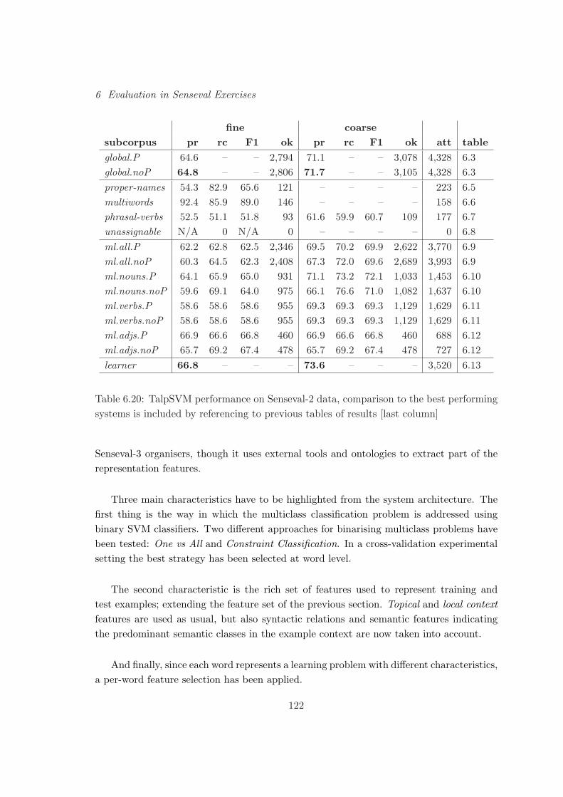
6 Evaluation in Senseval Exercises
fine coarsesubcorpus pr rc F1 ok pr rc F1 ok att tableglobal.P 64.6 – – 2,794 71.1 – – 3,078 4,328 6.3global.noP 64.8 – – 2,806 71.7 – – 3,105 4,328 6.3proper-names 54.3 82.9 65.6 121 – – – – 223 6.5multiwords 92.4 85.9 89.0 146 – – – – 158 6.6phrasal-verbs 52.5 51.1 51.8 93 61.6 59.9 60.7 109 177 6.7unassignable N/A 0 N/A 0 – – – – 0 6.8ml.all.P 62.2 62.8 62.5 2,346 69.5 70.2 69.9 2,622 3,770 6.9ml.all.noP 60.3 64.5 62.3 2,408 67.3 72.0 69.6 2,689 3,993 6.9ml.nouns.P 64.1 65.9 65.0 931 71.1 73.2 72.1 1,033 1,453 6.10ml.nouns.noP 59.6 69.1 64.0 975 66.1 76.6 71.0 1,082 1,637 6.10ml.verbs.P 58.6 58.6 58.6 955 69.3 69.3 69.3 1,129 1,629 6.11ml.verbs.noP 58.6 58.6 58.6 955 69.3 69.3 69.3 1,129 1,629 6.11ml.adjs.P 66.9 66.6 66.8 460 66.9 66.6 66.8 460 688 6.12ml.adjs.noP 65.7 69.2 67.4 478 65.7 69.2 67.4 478 727 6.12learner 66.8 – – – 73.6 – – – 3,520 6.13
Table 6.20: TalpSVM performance on Senseval-2 data, comparison to the best performingsystems is included by referencing to previous tables of results [last column]
Senseval-3 organisers, though it uses external tools and ontologies to extract part of therepresentation features.
Three main characteristics have to be highlighted from the system architecture. Thefirst thing is the way in which the multiclass classification problem is addressed usingbinary SVM classifiers. Two different approaches for binarising multiclass problems havebeen tested: One vs All and Constraint Classification. In a cross-validation experimentalsetting the best strategy has been selected at word level.
The second characteristic is the rich set of features used to represent training andtest examples; extending the feature set of the previous section. Topical and local contextfeatures are used as usual, but also syntactic relations and semantic features indicatingthe predominant semantic classes in the example context are now taken into account.
And finally, since each word represents a learning problem with different characteristics,a per-word feature selection has been applied.
122
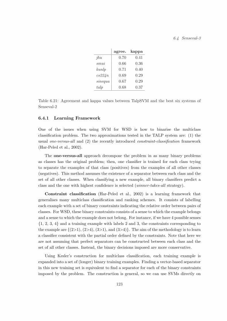
6.4 Senseval-3
agree. kappajhu 0.70 0.41smui 0.66 0.36kunlp 0.71 0.40cs224n 0.69 0.29sinequa 0.67 0.29talp 0.68 0.37
Table 6.21: Agreement and kappa values between TalpSVM and the best six systems ofSenseval-2
6.4.1 Learning Framework
One of the issues when using SVM for WSD is how to binarise the multiclassclassification problem. The two approximations tested in the TALP system are: (1) theusual one-versus-all and (2) the recently introduced constraint-classification framework(Har-Peled et al., 2002).
The one-versus-all approach decompose the problem in as many binary problemsas classes has the original problem; then, one classifier is trained for each class tryingto separate the examples of that class (positives) from the examples of all other classes(negatives). This method assumes the existence of a separator between each class and theset of all other classes. When classifying a new example, all binary classifiers predict aclass and the one with highest confidence is selected (winner-takes-all strategy).
Constraint classification (Har-Peled et al., 2002) is a learning framework thatgeneralises many multiclass classification and ranking schemes. It consists of labellingeach example with a set of binary constraints indicating the relative order between pairs ofclasses. For WSD, these binary constraints consists of a sense to which the example belongsand a sense to which the example does not belong. For instance, if we have 4 possible senses{1, 2, 3, 4} and a training example with labels 2 and 3, the constraints corresponding tothe example are {(2>1), (2>4), (3>1), and (3>4)}. The aim of the methodology is to learna classifier consistent with the partial order defined by the constraints. Note that here weare not assuming that perfect separators can be constructed between each class and theset of all other classes. Instead, the binary decisions imposed are more conservative.
Using Kesler’s construction for multiclass classification, each training example isexpanded into a set of (longer) binary training examples. Finding a vector-based separatorin this new training set is equivalent to find a separator for each of the binary constraintsimposed by the problem. The construction is general, so we can use SVMs directly on
123

6 Evaluation in Senseval Exercises
the expanded training set to solve the multiclass problem. See Har-Peled et al. (2002) fordetails.
6.4.2 Features
The basic feature set is that detailed in section 6.3.2, with a few extensions. Local and topicfeatures are the same. Knowledge-based features have been extended by using the formulain section 6.2.1 to other semantic resources into the Multilingual Central Repository (Mcr)(Atserias et al., 2004) of the Meaning Project: Sumo labels, WordNet Lexicographic Files,and EuroWordNet Top Ontology. Also, it has been extended with features codifying theoutput of Yarowsky’s dependency pattern extractor11.
Appendix B details part of the output of the feature extractor for an example ofSenseval-2 corpus.
Since the set of features is highly redundant, a selection process has been applied. Itis detailed in the next section.
6.4.3 Experimental Setting
For each binarisation approach, we performed a feature selection process consisting of twoconsecutive steps:
• Feature selection by PoS: Using the Senseval-2 corpus, an exhaustive selection ofthe best set of features for each particular Part-of-Speech has been performed. Thesefeature sets are taken as the initial sets in the feature selection process of Senseval-3.Table 6.22 shows which features have been selected for each Part-of-Speech (seeappendix B for an explanation of the labels of the first two columns of the table).
• Feature selection by word: We applied a forward(selection)-backward(deletion)two step procedure to obtain the best feature selection per word. For eachword, the process starts with the best feature set obtained in the previous stepaccording to its Part-of-Speech. In the selection part, we consider those featuresnot selected during feature selection by PoS, adding all features which producesome improvement. During deletion, we consider only those features selectedduring feature selection by PoS, removing all features whose deletion produces someimprovement. Although this addition-deletion procedure could be iterated untilachieving no further improvements, we only performed a unique iteration becauseits computational overhead.
124

6.4 Senseval-3
feature feature group nouns verbs adjsform form X X -all locat X X Xpos coll - X Xform coll X - -lemma coll X X Xall coll2 X X Xform noun/verb first sent. - X -form adj first sent. - X Xlemma noun/verb/adv first sent. X X Xlemma adj first sent. X - Xform noun/verb/adv first ±10w X X Xform adj first ±10w X X -lemma first ±10w X X Xform topic sent. - - Xlemma topic sent. X X -all topic ±10w - - Xform sbig sent. - X Xlemma sbig sent. - - Xall sbig ±10w X X Xform comb sent. - X -form comb ±10w - X -lemma comb ±10w X X X- f sumo X X X- a sumo X X X- f semf - X -- a semf X X X- f tonto X - -- a tonto X X X- f magn X X X- a magn X X X- tgt mnp X X X- rels mnp X X Xall yar * X X X
Table 6.22: Selected Features per Part-of-Speech.
125

6 Evaluation in Senseval Exercises
The result of this preprocess is the selection of the best binarisation approach with itsbest feature set for each word.
Regarding the implementation details of the system, we used again SVMlight (Joachims,2002). A simple lineal kernel with a regularisation C value of 0.1 was applied. Thisparameter was empirically decided on the basis of our previous experiments on theSenseval-2 corpus. Again, previous tests using non-linear kernels did not provide betterresults. The selection of the best feature set and the binarisation scheme per worddescribed above, have been performed using 5-fold cross-validation on the Senseval-3training set. The five partitions of the training set were obtained maintaining, as muchas possible, the initial distribution of examples per sense (using the stratified samplingscheme).
After several experiments considering the U label as an additional regular class, wefound that we obtained better results by simply ignoring it. Then, if a training examplewas tagged only with this label, it was removed from the training set. If the examplewas tagged with this label and others, the U label was also removed from the learningexample. In that way, the TALP system do not assigns U labels to the test examples.Due to lack of time, the TALP system presented at the competition time did not includea complete model selection for the constraint classification binarisation setting. Moreprecisely, 14 words were processed within the complete model selection framework, and43 were adjusted with only the one-vs-all approach with feature selection but not theconstraint classification approach. After the competition was closed, we implemented theconstraint classification setting more efficiently and we reprocessed again the data.
6.4.4 Evaluation
Table 6.23 shows the accuracy obtained in the training set by 5 fold cross-validation.OVA(base) stands for the results of the one-versus-all approach on the starting featureset; CL(base) for the constrain-classification on the starting feature set; and OVA(best)and CL(best) mean one-versus-all and constraint-classification with their respective featureselection. Final stands for the full architecture on the training set and SE3 for the resultsobtained at competition time12.
Globally, feature selection consistently improves the accuracy in 3 points (both inOVA and CL). Constraint-classification is slightly better than one-vs-all approach; butthe Final (the full architecture) results shows that it is not true for all the words. Finally,the combined feature selection increases the accuracy in half a point.
11This software was kindly provided by David Yarowsky’s group, from Johns Hopkins University.12Only 14 words where processed at competition time due to lack of time.
126

6.4 Senseval-3
method acc.OVA(base) 72.38CL(base) 72.28OVA(best) 75.27CL(best) 75.70SE3 75.62Final 76.02
Table 6.23: Results on the Senseval-3 5 fold cross-validation training set (accuracy in%)
Table 6.24 shows the official results of the system. SE3 means the official result13,Final means the complete architecture, and Best means the winner of the competition.
measure SE3 Final Bestfine 71.3 71.6 72.9coarse 78.2 78.2 79.3
Table 6.24: Official Senseval-3 Results (accuracy in%)
However, when testing the complete architecture on the official test set, we obtainedan accuracy decrease of more than 4 points. Nevertheless, the system obtained highcompetitive results: ranking in the 7th team position, at only 1.3 points on fine-grainedaccuracy and by 1.1% on coarse-grained accuracy below the winner.
6.4.5 Extending the Feature Selection process
This section presents the results of the application of three new feature selection methodsusing the Senseval-3 corpora.
The first method is a greedy iterative process (hereinafter bf ) in which the best feature(in accuracy) is selected at each step. The initial features of this method is the empty set.This approximation is local and greedy. Sometimes, a pair of features would be selectedin order to improve the overall. And once a feature is selected it can not be deleted. Avariant of this method consisting of using as initial set those in table 6.22 has been calledwbf.
The third process, hill climbing (hereinafter hc), aims to avoid the problem of selectinga bad feature. It is also a greedy iterative process. First and second steps are like the
13Only 14 words were processed with the full architecture.
127

6 Evaluation in Senseval Exercises
previous one. That is, the process selects the best two features in two iterations. From thethird step further, each step looks for the best feature (in accuracy) to add and the bestto delete (if it exists a feature that increases the accuracy in being deleted). The initialset of this method is also the empty set.
Evaluation
Table 6.25 shows the result of the three feature selection methods on the Senseval-3 corporafor nouns, verbs, adjectives and overall. The first method (wrd) is the one we presentedto the Senseval-3 event, achieving a fine-grained accuracy of 71.6 and a coarse one of 78.2.Although every procedure achieves the best performance on some words, the best overallsystem is wrd. That is, none of feature selection methods improved the original results.
pos wrd bf hc wbfnouns 71.9 72.1 70.8 69.2 72.0verbs 72.3 73.0 72.1 72.3 72.8adjectives 50.3 49.1 49.7 44.0 49.1all 71.2 71.6 70.6 69.8 71.5
Table 6.25: Fine-grained Results.
The basic aim of table 6.26 is showing the impact on accuracy of the feature selectionprocedures for the seven first words of Senseval-3 English Lexical Sample corpus. ova-wrdstands for one versus all binarisation plus wrd feature selection procedure, cc-wrd forconstraint classification plus wrd selection, and so on. top, loc, dom and syn standsrespectively for topical, local, domain and syntactical features. So, the four first columnsof the table show the number of words for which the method has selected some of thosefeatures. The last column (avg) shows the average number of features selected by themethod.
It seems that generally one versus all selects more features than constrain classification.wrd and wbf feature selection procedures gather much more features (around 50 types ofthem) than the others (less than 20). While wrd and wbf methods start with a largefeature set (approximately 40 feature types depending of the part-of-speech), bf and hcbegin with the empty set. This explains the differences between them. Furthermore, bfselects the double number of features than hc because hc deletes features in its iterativeprocess.
Regarding the 4 clusters of features, all methods have selected local features for all the
128

6.5 Conclusions
loc top dom syn avgova-wrd 7 7 7 7 49.7cc-wrd 7 7 7 7 48.6ova-bf 7 7 4 4 16.1cc-bf 7 4 4 3 9.9ova-hc 7 6 5 4 17.7cc-hc 7 2 3 3 10.4ova-wbf 7 7 7 7 48.6cc-wbf 7 7 7 7 49.9
Table 6.26: Features Selection Information.
words. The domain features from the MCR are equally selected as topical features andselected more often than syntactical features.
6.5 Conclusions
We have participated in the English Lexical Sample task of last two editions of Sensevalinternational evaluation exercises. Our systems have achieved a very high position in bothcompetitions. That is, they are part of the State-of-the-Art in supervised WSD systems.
At Senseval-2, we proposed a system based on LazyBoosting, an improved versionof the AdaBoost.MH. We enriched the typical local and topical context with domaininformation. After the exercise, we have studied the outputs of the six best system andproposed a new system based on SVM that outperformed all the six systems presented atthe competition.
At Senseval-3, we proposed and tested a supervised system in which the examples arerepresented through a very rich and redundant set of feature (using the information contentintegrated within the Multilingual Central Repository of the Meaning project), and whichperforms some specialised selection of features and multiclass binarisation process foreach word. All these features lead to a better system able to be automatically configuredfor every word. The main drawback of the approach presented in this work is the highcomputational overhead of the feature selection process for every word.
The system based on Support Vector Machines and a rich set of features has a veryhigh competitive performance. The features based on domains bring new complementaryand useful information.
This work suggests some promising lines to be studied in detail: 1) Searching new waysof representing the examples: for instance, the learning algorithms could use the output
129

6 Evaluation in Senseval Exercises
information of unsupervised systems as features; and 2) improving the per-word featureselection: for instance, some other procedures should be tested, such as descendent hillclimbing14.
Finally, there are some open questions: 1) Which set of features better represent eachsense of each word? 2) How do we have to binarise the multiclass problem? And 3) Howdo we have to treat examples with more than one possible sense (multilabel assignments)?
14That is, starting from the full feature set and deleting features at each iteration.
130

Chapter 7
Conclusions
7.1 Summary
Word Sense Disambiguation is one of the tasks for dealing with NLP semantics. Firstreferences on Lexical Ambiguity are sixty years old. Despite the work devoted to theproblem, it can be said that no large-scale broad-coverage accurate WSD system has beenbuilt up to date (Kilgarriff and Rosenzweig, 2000). Therefore, WSD is one of the mostimportant open problems in NLP, with current state-of-the-art accuracy in the 60-70%range. Machine Learning classifiers are effective, but, due to the knowledge acquisitionbottleneck, they will not be feasible until reliable methods for acquiring large sets oftraining examples with a minimum human annotation effort will be available. Theseautomatic methods for helping in the collection of examples should be robust to noisy dataand changes in sense frequency distributions and corpus domain (or genre). The adequateML algorithms used to induce the WSD classifiers should be also noise-tolerant (both inclass-label and feature values), easy to adapt to new domains, robust to overfitting, andefficient for learning thousands of classifiers in very large training sets and feature spaces.
Many NLP researchers consider word sense ambiguity as a central problem forseveral Human Language Technology applications, (e.g., Machine Translation, InformationExtraction and Retrieval, etc.). This is also the case for most of the associated sub-tasks,for instance, reference resolution and parsing. For this reason, many international researchgroups have been actively working on WSD during last years, using a wide range ofapproaches. This can be noticed throughout the recent publications in the main NLPconferences and journals (including special issues on the WSD task), the organisation ofspecialised conferences on this topic, a number of current NLP research projects includingWSD among their goals, and the increasing number of participants in the different editions
131

7 Conclusions
of the Senseval international competitions.
The Senseval international evaluation exercises (organised by the ACL SIGLEX)introduced two main evaluation approaches on Word Sense Disambiguation. The LexicalSample proposes to disambiguate only a word in a sentence. Typically these words arethe most polysemous and difficult to solve and the Senseval organisers provide a set oftraining examples for each word. The All Words task proposes the evaluation on all theopen-class words of a text, and the Senseval organisers do not provide training examples.
The Best Systems at the English Lexical Sample task on the last Senseval editionsobtained accuracy results lower than 75%. Obviously, this figures are not useful forpractical purposes. We think that the best way to improve the current systems is to exploitthe representation of the examples with linguistic knowledge that is not currently availablein wide-coverage lexical knowledge bases. We refer, for instance, to sub-categorisationframes, syntactic structure, selectional preferences, and domain information. That is, anin depth study of the features is needed (the better we represent examples, the betterlearning systems will be obtained). One of the biggest problems of this approach is thedependency of the classifiers on the training corpora. We need an in depth study on thedependency on the corpora and a way to develop general corpora or effective and simpleways to adapt to new application domains.
The Best Systems at the All-words task on last Senseval edition obtained accuracyresults near 65%. Following the supervised approach, we need a large amount of labelledcorpora to build a broad coverage Word Sense Tagger; which are very expensive. Themost promising line to tackle this problem is the application of bootstrapping techniquesto profit from unlabelled examples. This is one of the interesting current research lineson Word Sense Disambiguation field and other NL-related tasks. Moreover, future WSDsystems will need to automatically detect and collapse spurious sense distinctions, as wellas to discover, probably in an on-line learning setting, occurrences of new senses in runningtext.
We also think that it might be very useful to develop more complex systems dealingwith Semantics from several points of view, like systems based on Semantic Parsing.
Finally, we think that there are some general outstanding problems within Word SenseDisambiguation dealing with semantics. The most important one is the demonstration, ona real application, of the usefulness of Word Sense Disambiguation. Another open issue isthe utility of WSD in semantics to develop Natural Language Understanding Systems.
132

7.2 Contributions
7.2 Contributions
This section summarises the main contributions of the thesis. We have grouped thembased on the same chapters of this document:
Comparison of supervised ML algorithms for WSD: First, we have performed adirect comparison of the most used algorithms by the community. As a complementaryissue, we have clarified some confusing information on the literature and developed someimprovements on the adaptation (representation of the information and efficiency) ofsome algorithms. We have empirically showed that the best systems on Word SenseDisambiguation data are those based on margin maximisation. This evaluation is basednot only on accuracy values, but also on agreement and Kappa statistics.
Cross-corpora evaluation and adaptation to new domains: The experiments ofchapter 4 have empirically shown the dependency of the classifiers based on MachineLearning to the training corpora. This issue has to be solved in order to develop a realand useful Supervised Word Sense tagger. This is an important issue because until knowingthe way of building full general corpora, training less dependant classifiers, or adaptingclassifiers to new domains; the only taggers we can build are those based on particulardomains.
Data scarceness, bootstrapping: The contributions here are the application ofTransductive Support Vector Machines and the Greedy Agreement bootstrappingalgorithm to Word Sense Disambiguation. The first approach does not seem to workon this problem appropriately. Instead, the Greedy Agreement algorithm shows betterperformance. The first experiments seem to indicate a promising future line of research.
International evaluation exercises: We have participated to the English LexicalSample task of both Senseval-2 and 3 competitions obtaining fairly good results. AtSenseval-2 our system got the fifth position at 4.8% of accuracy from the first one, andat Senseval-3 it got the seventh position at only 1.6% of accuracy. In both cases oursystem was within the set of best performing systems. That is, our systems are among theState-of-the-Art systems on Word Sense Disambiguation. Improving the systems involvedin Senseval exercises have produced: a comparative study of the six best systems fromSenseval-2, and some improvements of the learning systems presented at competition time:1) the addition of new useful features, such as those based on domain information; 2) the
133

7 Conclusions
application of feature selection procedures, and the comparison between them; and 3)the application of different ways of binarising the multiclass problem when using binaryclassifiers, such as SVM.
7.3 Publications
This section lists the publications ordered by the contribution topics of the previoussection:
Comparison of supervised ML algorithms for WSD:
G. Escudero, L. Marquez, and G. Rigau. Boosting Applied to Word SenseDisambiguation. In Proceedings of the 12th European Conference onMachine Learning, ECML, 2000. Explained in section 3.4.
G. Escudero, L. Marquez, and G. Rigau. Naive Bayes and Exemplar-BasedApproaches to Word Sense Disambiguation Revisited. In Proceedingsof the 14th European Conference on Artificial Intelligence, ECAI, 2000.Explained in section 3.3.
L. Marquez, G. Escudero, D. Martınez, and G. Rigau. Machine LearningMethods for WSD. chapter of the book Word Sense Disambiguation:Algorithms, Applications, and Trends. E. Agirre and P. Edmonds, editors.Kluwer, 2006. Explained in section 3.5.
Cross-corpora evaluation and adaptation to new domains:
G. Escudero, L. Marquez, and G. Rigau. A Comparison between SupervisedLearning Algorithms for Word Sense Disambiguation. In Proceedings of the4th Computational Natural Language Learning Workshop, CoNLL, 2000.Explained in chapter 4.
G. Escudero, L. Marquez, and G. Rigau. An Empirical Study of theDomain Dependence of Supervised Word Sense Disambiguation Systems.In Proceedings of the joint SIGDAT Conference on Empirical Methods inNatural Language Processing and Very Large Corpora, EMNLP/VLC, 2000.Explained in chapter 4.
134

7.4 Further Work
Data scarceness: bootstrapping:
G. Escudero and L. Marquez. Transductive Approach using Support VectorMachines on Labelled and Unlabelled Data. Deliverable WP6.5 of theMEANING Project (IST-2001-34460), 2003. Explained in section 5.1.
International evaluation exercises:
G. Escudero, L. Marquez, and G. Rigau. Using Lazy Boosting for WordSense Disambiguation. In Proceedings of the 2nd International Workshopan Evaluating Word Sense Disambiguation Systems, Senseval-2, 2001.Explained in section 6.2.
G. Escudero, L. Marquez, and G. Rigau. TALP System for the EnglishLexical Sample Task. In Proceedings of the 3rd International Workshopan Evaluating Word Sense Disambiguation Systems, Senseval-3, 2004.Explained in section 6.4.
Lexical/semantic resources for NLP:
L. Villarejo, J. Atserias, G. Escudero and G. Rigau. First Release ofthe Multilingual Central repository of MEANING. In Proceedings of theSEPLN, 2003.
L. Benıtez, S. Cervell, G. Escudero, M. Lopez, G. Rigau and M. Taule.Methods and tools for building the Catalan WordNet. In LREC Workshop:Language Resources for European Minority Languages, 1998.
L. Benıtez, S. Cervell, G. Escudero, M. Lopez, G. Rigau and M. Taule. WebWordNet Interface (Un sistema para el desarrollo de WordNets a traves dela Web). In Proceedings of the SEPLN, 1998.
7.4 Further Work
This section is devoted to explain the current work and further research lines that we planto address:
• First, the representation of the examples. Which is the best way to represent theexamples? Which is the best feature selection procedure?
135

7 Conclusions
• The second research line is the application of bootstrapping techniques to WordSense Disambiguation in order to increase, in a simple way, the amount of trainingexamples; alleviating the data scarceness problem. We also are interested in on-linelearning classifiers able to adapt to new domains.
• The third line is the integration of Semantic Parsing models within Word SenseDisambiguation classifiers in order to develop a better and complementary hybridsystem to deal with both tasks.
• And finally, we want to continue participating in next editions of Sensevalcompetitions, in both Lexical Sample and All-word tasks, for English, Catalan andSpanish languages.
136

Bibliography
S. Abney. Bootstrapping. In Proceedings of the Annual Meeting of the Association forComputational Linguistics, ACL, 2002.
S. Abney. Understanding the Yarowsky Algorithm. Computational Linguistics, 30(3),2004.
S. Abney, R. E. Schapire, and Y. Singer. Boosting Applied to Tagging and PP–attachment.In Proceedings of the SIGDAT Conference on Empirical Methods and Very LargeCorpora, EMNLP/VLC, 1999.
E. Agirre, O. Lopez de Lacalle Lekuona, and D. Martınez. Exploring feature spaceswith SVD and unlabeled data for Word Sense Disambiguation. In Proceedings of theInternational Conference: Recent Advances in Natural Language Processing, RANLP,2005.
E. Agirre and P. Edmonds, editors. Word Sense Disambiguation: Algoristhms,Applications, and Trends. Kluwer, 2006.
E. Agirre and D. Martınez. Exploring Automatic Word Sense Disambiguation withDecision Lists and the Web. In Proceedings of the COLING workshop: SemanticAnnotation and Intelligent Annotation, 2000.
E. Agirre and D. Martınez. Knowledge Sources for WSD. In Proceedings of theInternational TSD Conference, 2001.
E. Agirre and D. Martınez. Smoothing and Word Sense Disambiguation. In Proceedingsof Espana for Natural Language Processing (EsTAL), 2004a.
E. Agirre and D. Martınez. The Basque Country University system: English and Basquetasks. In Proceedings of the International Workshop on the Evaluation of Systems forthe Semantic Analysis of Text, Senseval–3, 2004b.
137
BIBLIOGRAPHY
E. Agirre and D. Martınez. Unsupervised WSD based on automatically retrieved examples:The importance of bias. In Proceedings of the International Conference on EmpiricalMethods in Natural Language Processing, EMNLP, 2004c.
E. Agirre and G. Rigau. A Proposal for Word Sense Disambiguation using ConceptualDistance. In Proceedings of the International Conference: Recent Advances in NaturalLanguage Processing, RANLP, 1995.
E. Agirre and G. Rigau. Word Sense Disambiguation Using Conceptual Density. InProceedings of the International Conference on Computational Linguistics, COLING,1996.
H. Alshawi and D. Carter. Training and scaling preference functions for disambiguation.Computational Linguistics, 20(4), 1994.
R. K. Ando and T. Zhang. A High–Performance Semi–Supervised Learning Methodfor Text Chunking. In Proceedings of the Annual Meeting of the Association forComputational Linguistics, ACL, 2005.
S. Argamon-Engelson and I. Dagan. Committee–based Sample Selection for ProbabilisticClassifiers. Journal of Artificial Intelligence Research, 11, 1999.
J. Atserias, B. Casas, E. Comelles, M. Gonzalez, L. Padro, and M. Padro. FreeLing 1.3:Syntactic and semantic services in an open-source NLP library. In Proceedings of the5th International Conference on Language Resources and Evaluation, LREC, 2006.
J. Atserias, S. Climent, J. Farreras, G. Rigau, and H. Rodrıguez. Combining MultipleMethods for the Automatic Construction of Multilingual WordNets. In Proceedings ofConference on Recent Advances in Natural Language Processing, RANLP, 1997.
J. Atserias, L. Villarejo, G. Rigau, E. Agirre, J. Carroll, B. Magnini, and P. Vossen.The MEANING Multilingual Central Repository. In Proceedings of the InternationalWordNet Conference, 2004.
Y. Bar-Hillel. The present status of automatic translation of languages. In F. L. Alt,editor, Advances in Computers. Academic Press, 1960.
E. Bauer and R. Kohavi. An Empirical Comparison of Voting Classification Algorithms:Bagging, Boosting and Variants. Machine Learning Journal. Special issue on IMLM forImproving and Scaling Machine Learning Algorithms, 1999.
A. Berger, S. Della Pietra, and V. Della Pietra. A Maximum Entropy Approach to NaturalLanguage Processing. Computational Linguistics, 22(1), 1996.
138

BIBLIOGRAPHY
A. Blum and T. Mitchell. Combining labeled and unlabeled data with co–training. InProceedings of the Workshop on Computational Learning Theory, COLT, 1998.
B. Boser, I. Guyon, and V. Vapnik. A Training Algorithm for Optimal Margin Classifiers.In Proceedings of the Workshop on Computational Learning Theory, COLT , 1992.
T. Brants. Internal and external tagsets in part-of-speech tagging. In Proceedings ofEuroSpeech, 1997.
L. Breiman. Arcing Classifers. The Annals of Statistics, 26(1), 1998.
E. Brill. Transformation–based Error–Driven Learning and Natural Language Processing:A Case Study in Part–of–Speech Tagging. Computational Linguistics, 21(4), 1995.
E. Briscoe and J. Carroll. Automatic extraction of subcategorization from corpora. InProceedings of the ACL Conference on Applied Natural Language Processing, 1997.
E. J. Briscoe. Lexical issues in natural language processing. In E. H. Klein andF. Veltman, editors, Natural Language and Speech Proceedings of the Symposium onNatural Language and Speech. Springer–Verlag, Berlin, 1991.
R. F. Bruce and J. M. Wiebe. Decomposable Modeling in Natural Language Processing.Computational Linguistics, 25(2), 1999.
C. Cabezas, P. Resnik, and J. Stevens. Supervised Sense Tagging using Support VectorMachines. In Proceedings of the International Workshop on Evaluating Word SenseDisambiguation Systems, 2001.
C. Cardie and R. J. Mooney. Guest Editors’ Introduction: Machine Learning and NaturalLanguage. Machine Learning (Special Issue on Natural Language Learning), 34, 1999.
J. Carletta. Assessing Agreement on Classification Tasks: the Kappa Statistic.Computational Linguistics, 22(2), 1996.
M. Carpuat, W. Su, and D. Wu. Augmenting Ensemble Classification for Word SenseDisambiguation with a Kernel PCA Model. In Proceedings of the InternationalWorkshop on the Evaluation of Systems for the Semantic Analysis of Text, Senseval–3,2004.
M. Carpuat and D. Wu. Word Sense Disambiguation vs. Statistical Machine Translation.In Proceedings of the Annual Meeting of the Association for Computational Linguistics,ACL, 2005.
139

BIBLIOGRAPHY
M. Castillo, F. Real, J. Atserias, and G. Rigau. The TALP Systems for DisambiguatingWordNet Glosses. In Proceedings of the International Workshop on the Evaluation ofSystems for the Semantic Analysis of Text, Senseval–3, 2004.
S. F. Chen. Building Probabilistic Models for Natural Language. PhD thesis, Center forResearch in Computing Technology. Harvard University, 1996.
T. Chklovski and R. Mihalcea. Building a Sense Tagged Corpus with Open Mind WordExpert. In Proceedings of the ACL workshop: Word Sense Disambiguation: RecentSuccesses and Future Directions, 2002.
J. Cohen. A coefficient of agreement for nominal scales. Educational and PsychologicalMeasurement, 20, 1960.
M. Collins. Parameter Estimation for Statistical Parsing Models: Theory and Practice ofDistribution–Free Methods. In To appear as a book chapter, 2002. Available at the webaddress: www.ai.mit.edu/people/mcollins.
M. Collins and Y. Singer. Unsupervised models for named entity classification. InProceedings of the joint SIGDAT Conference on Empirical Methods in Natural LanguageProcessing and Very Large Corpora, EMNLP/VLC, 1999.
C. Connine. Effects of sentence context and lexical knowledge in speech processing. InG. T. Altmann, editor, Cognitive models in speech processing. MIT Press, 1990.
S. Cost and S. Salzberg. A Weighted Nearest Neighbor Algorithm for Learning withSymbolic Features. Machine Learning, 10, 1993.
J. Cowie, J. Guthrie, and L. Guthrie. Lexical disambiguation using simulated annealing.In Proceedings of the International Conference on Computational Linguistics, COLING,1992.
E. Crestan, M. El-Beze, and C. de Loupy. Improving WSD with Multi–Level View ofContext Monitored by Similarity Measure. In Proceedings of the International Workshopon evaluating Word Sense Disambiguation Systems, 2001.
N. Cristianini and J. Shawe-Taylor. An Introduction to Support Vector Machines.Cambridge University Press, 2000.
W. Daelemans and V. Hoste. Evaluation of Machine Learning Methods for NaturalLanguage Processing Tasks. In Proceedings of the International Conference on LanguageResources and Evaluation, LREC, 2002.
140

BIBLIOGRAPHY
W. Daelemans, A. van den Bosch, and J. Zavrel. Forgetting Exceptions is Harmful inLanguage Learning. Machine Learning (Special Issue on Natural Language Learning),34, 1999.
W. Daelemans, J. Zavrel, K. van der Sloot, and A. van den Bosch. Timbl: Tilburg memorybased learner, version 4.0, reference guide. Technical Report, University of Antwerp,2001.
I. Dagan, Y. Karov, and D. Roth. Mistake–Driven Learning in Text Categorization. InProceedings of the Conference on Empirical Methods in Natural Language Processing,EMNLP, 1997.
S. Dasgupta, M. Littman, and D. McAllester. PAC generalization bounds for co–training.In Advances in Neural Infomation Processing Systems, NIPS, 2001.
J. Daude, L. Padro, and G. Rigau. Mapping Multilingual Hierarchies using RelaxationLabelling. In Proceedings of the Joint SIGDAT Conference on Empirical Methods innatural Language Processing and Very Large Corpora, EMNLP/VLC, 1999.
J. Daude, L. Padro, and G. Rigau. Magpping WordNets using Structural Information.In Proceedings of the Annual Meeting of the Association for Computational Linguistics,ACL, 2000.
J. Daude, L. Padro, and G. Rigau. A complete WN1.5 to WN1.6 Mapping. In Proceedingsof the NAACL Workshop: WordNet and Other Lexical Resources: Applications,Extensions and Customizations, 2001.
R. Lopez de Mantaras. A Distance–Based Attribute Selection Measure for Decission TreeInduction. Machine Learning, 6(1), 1991.
B. Decadt, V. Hoste, W. Daelemans, and A. van den Bosch. GAMBL, Genetic AlgorithmOptimization of Memory–Based WSD. In Proceedings of the International Workshopan Evaluating Word Sense Disambiguation Systems, Senseval–3, 2004.
T. G. Dietterich. Machine Learning Research: Four Current Directions. AI Magazine, 18(4), 1997.
T. G. Dietterich. Aproximate Statistical Tests for Comparing Supervised ClassificationLearning Algorithms. Neural Computation, 10(1), 1998.
T. G. Dietterich. An Experimental Comparison of Three Methods for ConstructingEnsembles of Decision Trees: Bagging, Boosting, and Randomization. MachineLearning, 40(2), 2000.
141

BIBLIOGRAPHY
R. O. Duda and P. E. Hart. Pattern Classification and Scene Analysis. John Wiley &Sons, 1973.
P. Edmonds and S. Cotton. Senseval–2: Overview. In Proceedings of the InternationalWorkshop on Evaluating Word Sense Disambiguation Systems, 2001.
S. Engelson and I. Dagan. Minimizing Manual Annotation Cost in SupervisedTraining from Corpora. In Proceedings of the Annual Meeting of the Association forComputational Linguistics, ACL, 1996.
G. Escudero and L. Marquez. Transductive Approach using Support Vector Machines onLabeled and Unlabeled Data. Technical report, Deliverable WP6.5 of the MEANINGProject (IST–2001–34460), 2003.
G. Escudero, L. Marquez, and G. Rigau. A Comparison between Supervised LearningAlgorithms for Word Sense Disambiguation. In Proceedings of the ComputationalNatural Language Learning Workshop, CoNLL, 2000a.
G. Escudero, L. Marquez, and G. Rigau. An Empirical Study of the Domain Dependenceof Supervised Word Sense Disambiguation Systems. In Proceedings of the joint SIGDATConference on Empirical Methods in Natural Language Processing and Very LargeCorpora, EMNLP/VLC, 2000b.
G. Escudero, L. Marquez, and G. Rigau. Boosting Applied to Word Sense Disambiguation.In Proceedings of the European Conference on Machine Learning, ECML, 2000c.
G. Escudero, L. Marquez, and G. Rigau. Naive Bayes and Exemplar–Based Approachesto Word Sense Disambiguation Revisited. In Proceedings of the European Conferenceon Artificial Intelligence, ECAI, 2000d.
G. Escudero, L. Marquez, and G. Rigau. Using Lazy Boosting for Word SenseDisambiguation. In Proceedings of the International Workshop an Evaluating WordSense Disambiguation Systems, Senseval–2, 2001.
G. Escudero, L. Marquez, and G. Rigau. TALP System for the English LexicalSample Task. In Proceedings of the International Workshop an Evaluating Word SenseDisambiguation Systems, Senseval–3, 2004.
C. Fellbaum, editor. WordNet. An Electronic Lexical Database. The MIT Press, 1998.
R. Florian, S. Cucerzam, C. Schafer, and D. Yarowsky. Combining Classifiers for WordSense Disambiguation. Natural Language Engineering, Special Issue on Evaluating WordSense Disambiguation Systems, 8(4), 2003.
142

BIBLIOGRAPHY
R. Florian and D. Yarowsky. Modelling consensus: Classifier combination for word sensedisambiguation. In Proceedings of the Conference on Empirical Methods in NaturalLanguage Processing, EMNLP, 2002.
W. N. Francis and H. Kucera. Frequency Analysis of English Usage: Lexicon andGrammar. Houghton Mifflin Company, 1982.
Y. Freund and R. E. Schapire. Experiments with a New Boosting Algorithm. InProceedings of the 13th International Conference on Machine Learning, ICML, 1996.
Y. Freund and R. E. Schapire. A Decision–theoric Generalization of On–line Learning andan Application to Boosting. Journal of Computer and System Sciences, 55(1), 1997.
A. Fujii, K. Inui, T. Tokunaga, and H. Tanaka. Selective Sampling for Example-BasedWord Sense Disambiguation. Computational Linguistics, 24(4), 1998.
W. Gale, K. W. Church, and D. Yarowsky. Estimating Upper and Lower Bounds on thePerformance of Word Sense Disambiguation. In Proceedings of the Annual Meeting ofthe Association for Computational Linguistics, ACL, 1992a.
W. Gale, K. W. Church, and D. Yarowsky. One Sense Per Discourse. In Proceedings ofthe DARPA Speech and Natural Language Workshop, 1992b.
W. Gale, K. W. Church, and D. Yarowsky. A Method for Disambiguating Word Senses ina Large Corpus. Computers and the Humanities, 26(5), 1993.
G. Grefenstette. Evaluation Techniques for Automatic Semantic Extraction: ComparingSyntatic and Window–based Approaches. In Proceedings of the ACL SIGLEX Workshopon Acquisition of Lexical Knowledge from Text, 1993.
C. Grozea. Finding optimal parameter settings for high performance word sensedisambiguation. In Proceedings of the International Workshop on the Evaluation ofSystems for the Semantic Analysis of Text, Senseval–3, 2004.
J. Guthrie, L. Guthrie, Y. Wilks, and H. Aidinejad. Subject–dependent Cooccurrence andWord Sense Disambiguation. In Proceedings of the Annual Meeting of the Associationfor Computational Linguistics, ACL, 1991.
S. Har-Peled, D. Roth, and D. Zimak. Constraint Classification for MulticlassClassification and Ranking. In Proceedings of the Workshop on Neural InformationProcessing Systems, 2002.
143
BIBLIOGRAPHY
S. M. Harabagiu and D. I. Moldovan. Knowledge Processing on an Extended WordNet.In C. Fellbaum, editor, WordNet: An Electronic Lexical Database and some of itsApplications. MIT Press, 1998.
V. Hoste, W. Daelemans, I. Hendrickx, and A. van den Bosch. Evaluating the Results ofa Memory–Based Word–Expert Approach to Unrestricted Word Sense Disambiguation.In Proceedings of the Workshop on Word Sense Disambiguation: Recent Successes andFuture Directions, 2002a.
V. Hoste, I. Hendrickx, W. Daelemans, and A. van den Bosch. Parameter Optimizationfor Machine–Learning of Word Sense Disambiguation. Natural Language Engineering,8(4), 2002b.
V. Hoste, A. Kool, and W. Daelemans. Classifier Optimization and Combination in theEnglish All Words Task. In Proceedings of the International Wordshop on EvaluatingWord Sense Disambiguation Systems, 2001.
N. Ide and J. Veronis. Introduction to the Special Issue on Word Sense Disambiguation:The State of the Art. Computational Linguistics, 24(1), 1998.
H. T. Ilhan, S. D. Kamvar, D. Klein, C. D. Manning, and K. Toutanova. CombiningHeterogeneous Classifiers for Word–Sense Disambiguation. In Proceedings of theInternational Workshop on evaluating Word Sense Disambiguation Systems, 2001.
T. Joachims. Text Categorization with Support Vector Machines: Learning with ManyRelevant Features. In Proceedings of the European Conference on Machine Learning,ECML, 1998.
T. Joachims. Transductive Inference for Text Classification using Support VectorMachines. In Proceedings of the Internacional Conference on Machine Learning, ICML,1999.
T. Joachims. Learning to Classify Text Using Support Vector Machines. Kluwer, 2002.
A. Kaplan. An Experimental Study of Ambiguity and Context. Mechanical Translation,2(2), 1950.
A. Kilgarriff. What is Word Sense Disambiguation Good For? In Proceedings of NLPPacific Rim Symposium, 1997.
A. Kilgarriff. Gold Standard Datasets for Evaluating Word Sense DisambiguationPrograms. Computer Speech and Language, Special Issue on Evaluation, 12(4), 1998a.
144

BIBLIOGRAPHY
A. Kilgarriff. SENSEVAL: An Exercise in Evaluating Word Sense DisambiguationPrograms. In Proceedings of the 1st Conference on Language Resources and Evaluation,LREC, 1998b.
A. Kilgarriff. English Lexical Sample Task Description. In Proceedings of the InternationalWorkshop on Evaluating Word Sense Disambiguation Systems, Senseval–2, 2001.
A. Kilgarriff and J. Rosenzweig. English SENSEVAL: Report and Results. In Proceedingsof the International Conference on Language Resources and Evaluation, LREC, 2000.
U. S. Kohomban and W. S. Lee. Learning semantic classes for word sense disambiguation.In Proceedings of the Annual Meeting of the Association for Computational Linguistics,ACL, 2005.
R. Krovetz and W. B. Croft. Lexical Ambiguity and Information Retrieval. ACMTransactions on Information Systems, 10(2), 1992.
T. Kudo and Y. Matsumoto. Chunking with Support Vector Machines. In Proceedingsof the Meeting of the North American Chapter of the Association for ComputationalLinguistics, NAACL, 2001.
C. Leacock, M. Chodorow, and G. A. Miller. Using Corpus Statistics and WordNetRelations for Sense Identification. Computational Linguistics, 24(1), 1998.
C. Leacock, G. Towell, and E. Voorhes. Towards Building Contextual Representationsof Word Sense Using Statistical Models. In Proceedings of SIGLEX Workshop onAcquisition of Lexical Knowledge from Text, 1993.
Y. K. Lee and H. T. Ng. An Empirical Evaluation of Knowledge Sources and LearningAlgorithms for Word Sense Disambiguation. In Proceedings of the Conference onEmpirical Methods in Natural Language Processing, EMNLP, 2002.
Y. K. Lee, H. T. Ng, and T. K. Chia. Supervised Word Sense Disambiguation with SupportVector Machines and Multiple Knowledge Sources. In Proceedings of the InternationalWorkshop on the Evaluation of Systems for the Semantic Analysis of Text, Senseval–3,2004.
D. B. Lenat and V. G. Ramanathan, editors. Building Large Knowledge–based Systems.Addison–Wesley, Reading, MA, US, 1990.
M. Lesk. Automated sense disambiguation using machine–readable dictionaries: How totell a pine cone from an ice cream cone. In Proceedings of the SIGDOC Conference,1986.
145

BIBLIOGRAPHY
D. Lewis and W. Gale. Training Text Classifiers by Uncertainty Sampling. In Proceedingsof the International ACM Conference on Research and Development in InformationRetrieval, 1994.
D. Lin. Dependency-based Evaluation of MiniPar. In Proceedings of Workshop on hteEvaluation of Parsing Systems, 1998.
B. Magnini and G. Cavaglia. Integrating Subject Field Codes into WordNet. In Proceedingsof the International Conference on Language Resources and Evaluation, LREC, 2000.
B. Magnini, C. Strapparava, G. Pezzulo, and A. Gliozzo. Using Domain Informationfor Word Sense Disambiguation. In Proceedings of the International Workshop onEvaluating Word Sense Disambiguation Systems, Senseval–2, 2001.
C. Manning and H. Schutze. Foundations of Statistical Natural Language Processing. TheMIT Press, 1999.
L. Marquez. Part–of–Speech Tagging: A Machine–Learning Approach based on DecisionTrees. PhD thesis, Departament de Llenguatges i Sistemes Informatics. UniversitatPolitecnica de Catalunya, 1999.
L.. Marquez, G. Escudero, D. Martınez, and G. Rigau. Word Sense Disambiguation:Algorithms, Applications and Trends, chapter Machine Learning Methods. Kluwer,2006.
L. Marquez, M. Taule, A. Martı, N. Artigas, M. Garcıa, F. Real, and D. Ferres. Senseval–3:The Spanish lexical sample task. In Proceedings of the International Workshop on theEvaluation of Systems for the Semantic Analysis of Text, Senseval–3, 2004a.
L. Marquez, M. Taule, A. Martı, M. Garcıa, F. Real, and D. Ferres. Senseval–3: TheSpanish lexical sample task. In Proceedings of the International Workshop on theEvaluation of Systems for the Semantic Analysis of Text, Senseval–3, 2004b.
D. Martınez. Supervised Word Sense Disambiguation: Facing Current Challenges. PhDthesis, Lengoaia eta Sistema Informatikoak Saila. Euskal Herriko Univertsitatea, 2004.
D. Martınez and E. Agirre. One Sense per Collocation and Genre/Topic Variations. InProceedings of the Joint SIGDAT Conference on Empirical Methods in Natural LanguageProcessing and Very Large Corpora, EMNLP/VLC, 2000.
D. Martınez, E. Agirre, and L. Marquez. Syntactic Features for High Precision WordSense Disambiguation. In Proceedings of International Conference on ComputationalLinguistics, COLING, 2002.
146

BIBLIOGRAPHY
R. Mihalcea. Bootstrapping Large Sense Tagged Corpora. In Proceedings of theInternational Conference on Languages Resources and Evaluation, LREC, 2002a.
R. Mihalcea. Instance Based Learning with Automatic Feature Selection Applied to WordSense Disambiguation. In Proceedings of the International Conference on ComputationalLinguistics, COLING, 2002b.
R. Mihalcea. Co–training and Self–training for Word Sense Disambiguation. In Proceedingsof the Conference on Natural Language Learning, CoNLL, 2004.
R. Mihalcea, T. Chklovski, and A. Kilgarriff. The Senseval–3 English Lexical SampleTask. In Proceedings of the International Workshop on the Evaluation of Systems forthe Semantic Analysis of Text, Senseval–3, 2004.
R. Mihalcea and E. Faruque. SenseLearner: Minimally Supervised Word SenseDisambiguation for All Words in Open Text. In Proceedings of the InternationalWorkshop on the Evaluation of Systems for the Semantic Analysis of Text, Senseval–3,2004.
R. Mihalcea and D. Moldovan. Pattern Learning and Active Feature Selection for WordSense Disambiguation. In Proceedings of the International Workshop on EvaluatingWord Sense Disambiguation Systems, Senseval–2, 2001.
R. Mihalcea and I. Moldovan. A Method for Word Sense Disambiguation of UnrestrictedText. In Proceedings of the 37th annual meeting of the Association for ComputationalLinguistics, ACL, 1999a.
R. Mihalcea and I. Moldovan. An Automatic Method for Generating Sense TaggedCorpora. In Proceedings of the Conference of the American Association for ArtificialIntelligence, AAAI, 1999b.
G. A. Miller, R. Beckwith, C. Fellbaum, D. Gross, and K. Miller. Five Papers on WordNet.Special Issue of International Journal of Lexicography, 3(4), 1990.
G. A. Miller, M. Chodorow, S. Landes, C. Leacock, and R. G. Thomas. Using a semanticconcordance for sense identification. In Proceedings of the ARPA Human LanguageTechnology Workshop, 1994.
G. A. Miller, C. Leacock, R. Tengi, and R. T. Bunker. A Semantic Concordance. InProceedings of the ARPA Workshop on Human Language Technology, 1993.
T. M. Mitchell. Machine Learning. McGraw Hill, 1997.
147

BIBLIOGRAPHY
R. J. Mooney. Comparative Experiments on Disambiguating Word Senses: An Illustrationof the Role of Bias in Machine Learning. In Proceedings of the Conference on EmpiricalMethods in Natural Language Processing, EMNLP, 1996.
M. Murata, M. Utiyama, K. Uchimoto, Q. Ma, and H. Isahara. Japanese Word SenseDisambiguation Using the Simple Bayes and Support Vector Machine Methods. InProceedings of the International Workshop an Evaluating Word Sense DisambiguationSystems, Senseval–2, 2001.
H. T. Ng. Exemplar-Base Word Sense Disambiguation: Some Recent Improvements. InProceedings of the Conference on Empirical Methods in Natural Language Processing,EMNLP, 1997a.
H. T. Ng. Getting Serious about Word Sense Disambiguation. In Proceedings of the ACLSIGLEX Workshop: Standardizing Lexical Resources, 1997b.
H. T. Ng and H. B. Lee. Integrating Multiple Knowledge Sources to Disambiguate WordSense: An Exemplar–based Approach. In Proceedings of the Annual Meeting of theAssociation for Computational Linguistics, ACL, 1996.
H. T. Ng, C. Y. Lim, and S. K. Foo. A Case Study on Inter–Annotator Agreement for WordSense Disambiguation. In Proceedings of the ACL SIGLEX Workshop: StandardizingLexical Resources, 1999.
G. Ngai and R. Florian. Transformation–based Learning in the Fast Lane. In Proceedingsof the Meeting of the North American Chapter of the Association for ComputationalLinguistics, NAACL, 2001.
I. Niles and A. Pease. Towards a Standard Upper Ontology. In Proceedings of the 2ndInternational Conference on Formal Ontology in Information Systems, FOILS’2001,2001.
T. Pedersen. A Decision Tree of Bigrams is an Accurate Predictor of Word Sense.In Proceedings of the North American Chapter of the Association for ComputationalLinguistics, NAACL, 2001.
T. Pedersen and R. Bruce. A New Supervised Learning Algorithm for Word SenseDisambiguation. In Proceedings of the National Conference on Artificial Intelligence,AAAI, 1997.
T. Pedersen and R. Bruce. Knowledge Lean Word–Sense Disambiguation. In Proceedingsof the Conference of the American Association for Artificial Intelligence, AAAI, 1998.
148

BIBLIOGRAPHY
M. Popescu. Regularized Least–Squares Classification for Word Sense Disambiguation.In Proceedings of the International Workshop on the Evaluation of Systems for theSemantic Analysis of Text, Senseval–3, 2004.
P. Procter. Longman’s Dictionary of Contemporary English. Longmans, Harlow, 1973.
J. R. Quinlan. C4.5 : Programs for Machine Learning. Morgan Kaufman, 1993.
J. R. Quinlan. Bagging, Boosting and C4.5. In Proceedings of the 13th AmericanConference on Artificial Intelligence, AAAI, 1996.
P. Resnik. Disambiguating noun groupings with respect to WordNet. In Proceedings ofthe ACL Workshop on Very Large Corpora, VLC’95, 1995.
P. Resnik and D. Yarowsky. A Perspective on Word Sense Disambiguation Methods andtheir Evaluation. In Proceedings of the SIGLEX Workshop: Tagging Text with LexicalSemantics: Why, What and How?, 1997.
F. Ribas. On Acquiring Appropriate Selectional Restrictions from Corpora Using aSemantic Taxonomy. PhD thesis, Departament de Llenguatges i Sistemes Informatics.Universitat Politecnica de Catalunya, 1995.
S. Richardson. Determining Similarity and Inferring Relations in a Lexical KnowledgeBase. PhD thesis, The City University of New York, New York, 1997.
G. Rigau. Automatic Acquisition of Lexical Knowledge from MRDs. PhD thesis,Departament de Llenguatges i Sistemes Informatics. Universitat Politecnica deCatalunya, 1998.
G. Rigau, J. Atserias, and E. Agirre. Combining Unsupervised Lexical Knowledge Methodsfor Word Sense Disambiguation. In Proceedings of the Annual Meeting of the Associationfor Computational Linguistics, Joint ACL/EACL, 1997.
R. L. Rivest. Learning Decision Lists. Machine Learning, 2, 1987.
G. Salton. Automatic Information Retrieval. McGraw Hill, 1968.
G. Salton and M. McGill. Introduction to Modern Information Retrieval. McGraw Hill,1983.
K. Samuel. Lazy Transformation–Based Learning. In Proceedings of the 11th InternationalFlorida AI Research Symposium Conference, 1998.
R. E. Schapire. The Boosting Approach to Machine Learning: An Overview. In MSRIWorkshop on Nonlinear Estimation and Classification, 2002.
149

BIBLIOGRAPHY
R. E. Schapire and Y. Singer. Improved Boosting Algorithms Using Confidence–ratedPredictions. Machine Learning, 37(3), 1999.
R. E. Schapire and Y. Singer. Boostexter: A Boosting–based System for TextCategorization. Machine Learning, 39(2/3), 2000.
H. Schutze. Dimensions of Meaning. In Proceedings of Supercomputing, 1992.
H. Schutze and J. Pedersen. Information retrieval based on word senses. In Proceedingsof SDAIR, 1995.
S. Sekine. The Domain Dependence of Parsing. In Proceedings of the 5th of AppliedNatural Language Processing, ANLP, 1997.
S. Seneff. TINA, A natural language system for spoken language applications.Computational Linguistics, 18(1), 1992.
H. Seo, S. Lee, H. Rim, and H. Lee. KUNLP system using Classification InformationModel at Senseval–2. In Proceedings of the International Workshop on evaluating WordSense Disambiguation Systems, Senseval–2, 2001.
B. Snyder and M. Palmer. The English All–Words Task. In Proceedings of the InternationalWorkshop on the Evaluation of Systems for the Semantic Analysis of Text, Senseval–3,2004.
R. Sproat, J. Hirschberg, and D. Yarowsky. A corpus–based synthesizer. In Proceedingsof the International Conference on Spoken Language Processing, 1992.
M. Stevenson and Y. Wilks. The Interaction of Knowledge Sources in Word SenseDisambiguation. Computational Linguistics, 27(3):321–349, 2001.
C. Strapparava, A. Gliozzo, and C. Giuliano. Pattern Abstraction and Term Similarity forWord Sense Disambiguation: IRST at Senseval–3. In Proceedings of the InternationalWorkshop on the Evaluation of Systems for the Semantic Analysis of Text, Senseval–3,2004.
A. Suarez. Resolucion de la ambiguedad semantica de las palabras mediante modelos deprobabilidad de maxima entropıa. PhD thesis, Departamento de Lenguajes y SistemasInformaticos. Universidad de Alicante, 2004.
A. Suarez and M. Palomar. A Maximum Entropy–based Word Sense DisambiguationSystem. In Proceedings of the International Conference on computational Linguistics,COLING, 2002.
150

BIBLIOGRAPHY
M. Sussna. Word sense disambiguation for gree–text indexing using a massive semanticnetwork. In Proceedings of the International Conference on Information and KnowledgeBase Management, CIKM, 1993.
G. Towell and E. M. Voorhees. Disambiguating Highly Ambiguous Words. ComputationalLinguistics, 24(1), 1998.
V. N. Vapnik. Statistical Learning Theory. John Wiley, 1998.
S. Vazquez, R. Romero, A. Suarez, A. Montoyo, M. Garcıa, M. T. Martın, M. A. Garcıa,and L. A. Urena. The R2D2 team at Senseval–3. In Proceedings of the InternationalWorkshop on the Evaluation of Systems for the Semantic Analysis of Text, Senseval–3,2004.
J. Veronis. A study of polysemy judgements and inter–annotator agreement. In Programmeand advanced papers of the Senseval workshop, 1998.
E. Viegas, K. Mahesh, S. Nirenburg, and S. Beale. Semantics in Action. In P. Saint-Dizier,editor, Predicative Forms in Natural Language and in Lexical Knowledge Bases. KluwerAcademic Press, 1999.
L. Villarejo, L. Marquez, E. Agirre, D. Martınez, B. Magnini, C. Strapparava,D. McCarthy, A. Montoyo, and A. Suarez. The “Meaning” system on the Englishall–words task. In Proceedings of the International Workshop on the Evaluation ofSystems for the Semantic Analysis of Text, Senseval–3, 2004.
E. Voorhees. Using WordNet to disambiguate word senses for text retrieval. In Proceedingsof the Annual International ACM SIGDIR Conference on Research and Developmentin Information Retrieval, 1993.
P. Vossen, editor. EuroWordNet. A Multilingual Database with Lexical Semantic Networks.Kluwer Academic Publishers, 1998.
W. Weaver. Translation. Machine Translation of Languages, 1955.
Y. Wilks, D. Fass, C. Guo, J. McDonald, T. Plate, and B. Slator. Providing MachineTractable Dictionary Tools. In J. Pustejowsky, editor, Semantics and the Lexicon.Dordrecht, Kluwer Academic Publishers, 1993.
Y. Wilks and M. Stevenson. The Grammar of Sense: Is word–sense tagging much morethan part–of–speech tagging? Technical Report CS-96-05, University of Sheffield,Sheffield, UK, 1996.
T. Winograd. Understanding Natural Language. Academic Press, 1972.
151

BIBLIOGRAPHY
D. Yarowsky. Word sense disambiguation using statistical models of Roget’s categoriestrained on large corpora. In Proceedings of the International Conference onComputational Linguistics, COLING, 1992.
D. Yarowsky. Decision Lists for Lexical Ambiguity Resolution: Application to AccentRestoration in Spanish and French. In Proceedings of the Annual Meeting of theAssociation for Computational Linguistics, ACL, 1994.
D. Yarowsky. Three Machine Learning Algorithms for Lexical Ambiguity Resolution. PhDthesis, Department of Computer and Information Sciences. University of Pennsylvania,1995a.
D. Yarowsky. Unsupervised Word Sense Disambiguation Rivaling Supervised Methods.In Proceedings of the Annual Meeting of the Association for Computational Linguistics,ACL, 1995b.
D. Yarowsky. Homograph Disambiguation in Text–to–speech Synthesys. In J. P. OliveJ. T. H. van Santen, R. Sproat and J. Hirschberg, editors, Progress in Speech Synthesis.Springer–Verlag, 1997.
D. Yarowsky. Hierarchical Decision Lists for Word Sense Disambiguation. Computers andthe Humanities, 34(2), 2000.
D. Yarowsky, S. Cucerzan, R. Florian, C. Schafer, and R. Wicentowski. The JohnsHopkings Senseval–2 System Descriptions. In Proceedings of the International Workshopon evaluating Word Sense Disambiguation Systems, Senseval–2, 2001.
V. Yngve. Syntax and the Problem of Multiple Meaning. Machine Translation ofLanguages, 1955.
D. Yuret. Some Experiments with a Naive Bayes WSD System. In Proceedingsof the International Workshop an Evaluating Word Sense Disambiguation Systems,Senseval–3, 2004.
152
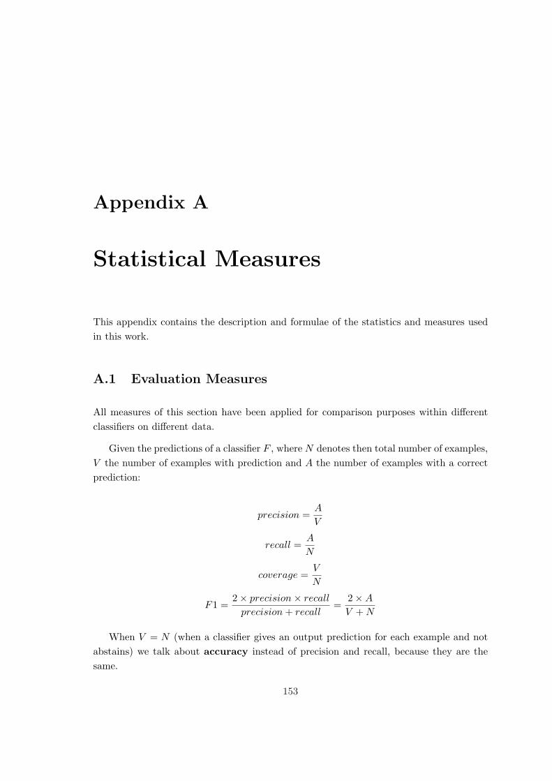
Appendix A
Statistical Measures
This appendix contains the description and formulae of the statistics and measures usedin this work.
A.1 Evaluation Measures
All measures of this section have been applied for comparison purposes within differentclassifiers on different data.
Given the predictions of a classifier F , where N denotes then total number of examples,V the number of examples with prediction and A the number of examples with a correctprediction:
precision =A
V
recall =A
N
coverage =V
N
F1 =2× precision× recall
precision + recall=
2×A
V + N
When V = N (when a classifier gives an output prediction for each example and notabstains) we talk about accuracy instead of precision and recall, because they are thesame.
153
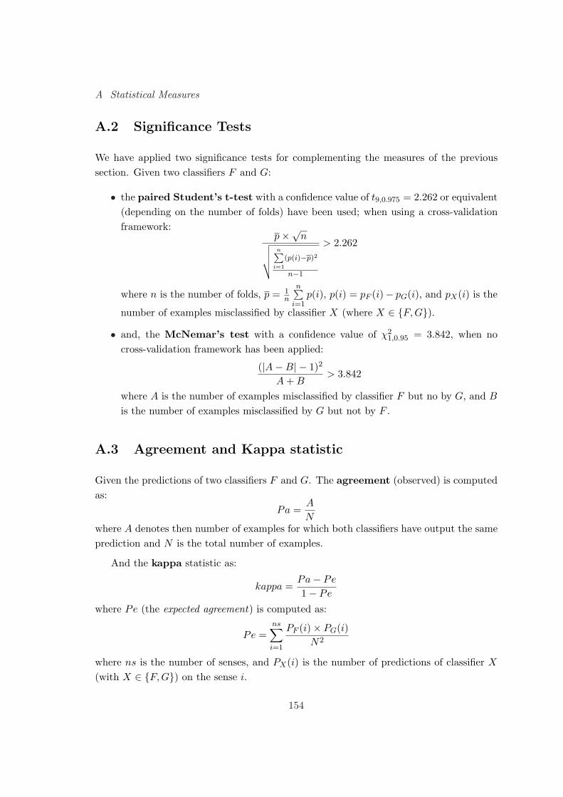
A Statistical Measures
A.2 Significance Tests
We have applied two significance tests for complementing the measures of the previoussection. Given two classifiers F and G:
• the paired Student’s t-test with a confidence value of t9,0.975 = 2.262 or equivalent(depending on the number of folds) have been used; when using a cross-validationframework:
p×√n√√√√n∑
i=1
(p(i)−p)2
n−1
> 2.262
where n is the number of folds, p = 1n
n∑i=1
p(i), p(i) = pF (i)− pG(i), and pX(i) is the
number of examples misclassified by classifier X (where X ∈ {F,G}).• and, the McNemar’s test with a confidence value of χ2
1,0.95 = 3.842, when nocross-validation framework has been applied:
(|A−B| − 1)2
A + B> 3.842
where A is the number of examples misclassified by classifier F but no by G, and B
is the number of examples misclassified by G but not by F .
A.3 Agreement and Kappa statistic
Given the predictions of two classifiers F and G. The agreement (observed) is computedas:
Pa =A
Nwhere A denotes then number of examples for which both classifiers have output the sameprediction and N is the total number of examples.
And the kappa statistic as:
kappa =Pa− Pe
1− Pe
where Pe (the expected agreement) is computed as:
Pe =ns∑
i=1
PF (i)× PG(i)N2
where ns is the number of senses, and PX(i) is the number of predictions of classifier X
(with X ∈ {F, G}) on the sense i.
154
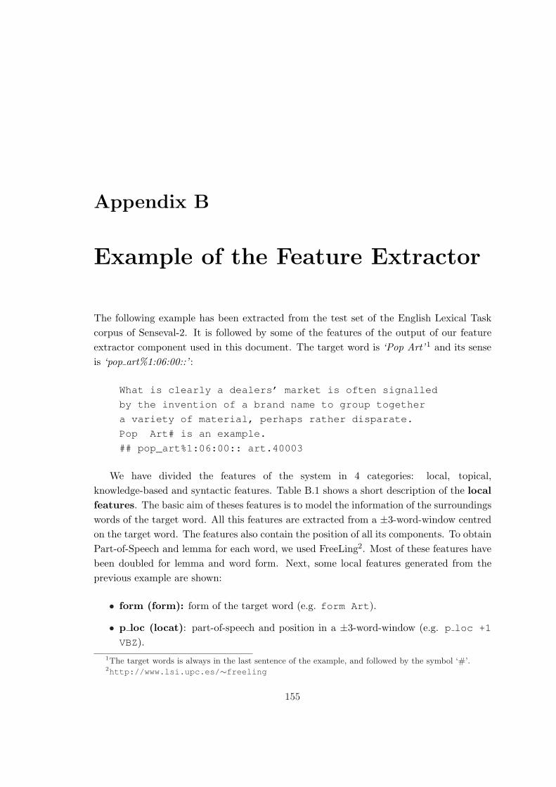
Appendix B
Example of the Feature Extractor
The following example has been extracted from the test set of the English Lexical Taskcorpus of Senseval-2. It is followed by some of the features of the output of our featureextractor component used in this document. The target word is ‘Pop Art’ 1 and its senseis ‘pop art%1:06:00::’ :
What is clearly a dealers’ market is often signalled
by the invention of a brand name to group together
a variety of material, perhaps rather disparate.
Pop Art# is an example.
## pop_art%1:06:00:: art.40003
We have divided the features of the system in 4 categories: local, topical,knowledge-based and syntactic features. Table B.1 shows a short description of the localfeatures. The basic aim of theses features is to model the information of the surroundingswords of the target word. All this features are extracted from a ±3-word-window centredon the target word. The features also contain the position of all its components. To obtainPart-of-Speech and lemma for each word, we used FreeLing2. Most of these features havebeen doubled for lemma and word form. Next, some local features generated from theprevious example are shown:
• form (form): form of the target word (e.g. form Art).
• p loc (locat): part-of-speech and position in a ±3-word-window (e.g. p loc +1
VBZ).1The target words is always in the last sentence of the example, and followed by the symbol ‘#’.2http://www.lsi.upc.es/∼freeling
155

B Example of the Feature Extractor
feat. descriptionform form of the target wordlocat all part-of-speech/forms/lemmas in the local contextcoll all collocations of two part-of-speech/forms/lemmascoll2 all collocations of a form/lemma and a part-of-speech (and
the reverse)first form/lemma of the first noun/verb/adjective/adverb on the
left/right of the target word
Table B.1: Local Feature Set
• f loc (locat): form and position in a ±3-word-window (i.e. f loc +1 is).
• l loc (locat): lemma and position in a ±3-word-window (e.g. l loc +1 be).
• ppcol (coll): part-of-speech collocations of every two words in a ±3-word-window(e.g. ppcol -1 NN +2 DT).
• ffcol (coll): form collocations of every two words (continuous or not) in a±3-word-window (e.g. ffcol -1 Pop +1 is).
• fpcol (coll2): form–part-of-speech collocations of every two words (continuous ornot) in a ±3-word-window (e.g. fpcol -1 Pop +1 VBZ).
• pfcol (coll2): part-of-speech–form collocations of every two words (continuous ornot) in a ±3-word-window (e.g. pfcol +1 VBZ +3 example).
• f fln (first): the form of the first noun on the left of the target word (e.g. f fln
Pop).
• l frv (first): the lemma of the first verb on the right of the target word (e.g. l frv
be).
Three types of topical features are shown in table B.2. Topical features try to obtainnon-local information from the words of the context. For each type, two overlapping setsof redundant topical features are considered: one extracted from a ±10-word-window andanother considering all the example. Next, it is shown some topical features generatedfrom previous example:
• f top (topic): bag of forms of the open-class-words in the example (e.g. f top
market).
156
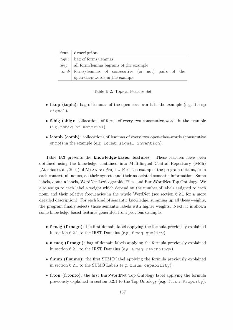
feat. descriptiontopic bag of forms/lemmassbig all form/lemma bigrams of the examplecomb forms/lemmas of consecutive (or not) pairs of the
open-class-words in the example
Table B.2: Topical Feature Set
• l top (topic): bag of lemmas of the open-class-words in the example (e.g. l top
signal).
• fsbig (sbig): collocations of forms of every two consecutive words in the example(e.g. fsbig of material).
• lcomb (comb): collocations of lemmas of every two open-class-words (consecutiveor not) in the example (e.g. lcomb signal invention).
Table B.3 presents the knowledge-based features. These features have beenobtained using the knowledge contained into Multilingual Central Repository (Mcr)(Atserias et al., 2004) of Meaning Project. For each example, the program obtains, fromeach context, all nouns, all their synsets and their associated semantic information: Sumolabels, domain labels, WordNet Lexicographic Files, and EuroWordNet Top Ontology. Wealso assign to each label a weight which depend on the number of labels assigned to eachnoun and their relative frequencies in the whole WordNet (see section 6.2.1 for a moredetailed description). For each kind of semantic knowledge, summing up all these weights,the program finally selects those semantic labels with higher weights. Next, it is shownsome knowledge-based features generated from previous example:
• f mag (f magn): the first domain label applying the formula previously explainedin section 6.2.1 to the IRST Domains (e.g. f mag quality).
• a mag (f magn): bag of domain labels applying the formula previously explainedin section 6.2.1 to the IRST Domains (e.g. a mag psychology).
• f sum (f sumo): the first SUMO label applying the formula previously explainedin section 6.2.1 to the SUMO Labels (e.g. f sum capability).
• f ton (f tonto): the first EuroWordNet Top Ontology label applying the formulapreviously explained in section 6.2.1 to the Top Ontology (e.g. f ton Property).
157

B Example of the Feature Extractor
feat. descriptionf sumo first sumo labela sumo all sumo labelsf semf first wn semantic file labela semf all wn semantic file labelsf tonto first ewn top ontology labela tonto all ewn top ontology labelsf magn first domain labela magn all domain labels
Table B.3: Knowledge-based Feature Set
feat. descriptiontgt mnp syntactical relations of the target word from miniparrels mnp all syntactical relations from miniparyar noun NounModifier, ObjectTo, SubjectTo for nounsyar verb Object, ObjectToPreposition, Preposition for verbsyar adjs DominatingNoun for adjectives
Table B.4: Syntactical Feature Set
• f smf (f semf): the first WordNet Semantic File label applying the formulapreviously explained in section 6.2.1 to the Semantic Files (e.g. f smf 42).
Finally, table B.4 describes the syntactic features which contains features extractedusing two different tools: Dekang Lin’s Minipar and Yarowsky’s dependency patternextractor. Next, it is shown some local features generated from previous example:
• mptgt (tgt mnp): minipar dependency relation to or from the target word (e.g.mptgt s:be).
• mprls (rels mnp): minipar dependency relations of the example (e.g. mprls
dealer:nn:market).
• NounModifier (yar noun): noun modifier (e.g. mosd NounModifier
Pop/NN).
• SubjectTo (yar noun): subject to (e.g. mosd SubjectTo is/VBZ).
158

Appendix C
Resources and Web References
1. Altavista Web Search Engine
http://www.altavista.com
2. British National Corpus
http://www.natcorp.ox.ac.uk
3. DSO Corpus
http://www.ldc.upenn.edu/Catalog/LDC97T12.html
4. EuroWordNet
http://www.illc.uva.nl/EuroWordNet/
5. FreeLing
http://garraf.epsevg.upc.es/freeling
6. Global WordNet Association
http://www.globalwordnet.org
7. hard, line and serve corpora
http://www.d.umn.edu/∼tpederse/data.html
8. interest corpus
http://crl.nmsu.edu/cgi-bin/Tools/CLR/clrcat#I9
9. LazyBoosting
http://www.lsi.upc.es/∼escudero
10. Linguistic Data Consortium (LDC)
http://www.ldc.upenn.edu
159
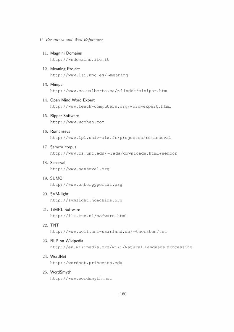
C Resources and Web References
11. Magnini Domains
http://wndomains.itc.it
12. Meaning Project
http://www.lsi.upc.es/∼meaning
13. Minipar
http://www.cs.ualberta.ca/∼lindek/minipar.htm
14. Open Mind Word Expert
http://www.teach-computers.org/word-expert.html
15. Ripper Software
http://www.wcohen.com
16. Romanseval
http://www.lpl.univ-aix.fr/projectes/romanseval
17. Semcor corpus
http://www.cs.unt.edu/∼rada/downloads.html#semcor
18. Senseval
http://www.senseval.org
19. SUMO
http://www.ontolgyportal.org
20. SVM-light
http://svmlight.joachims.org
21. TiMBL Software
http://ilk.kub.nl/sofware.html
22. TNT
http://www.coli.uni-saarland.de/∼thorsten/tnt
23. NLP on Wikipedia
http://en.wikipedia.org/wiki/Natural language processing
24. WordNet
http://wordnet.princeton.edu
25. WordSmyth
http://www.wordsmyth.net
160
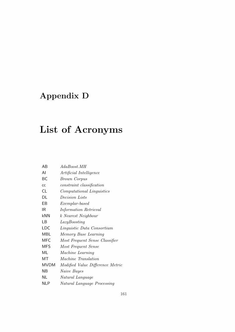
Appendix D
List of Acronyms
AB AdaBoost.MHAI Artificial IntelligenceBC Brown Corpuscc constraint classificationCL Computational LinguisticsDL Decision ListsEB Exemplar-basedIR Information RetrievalkNN k Nearest NeighbourLB LazyBoostingLDC Linguistic Data ConsortiumMBL Memory Base LearningMFC Most Frequent Sense ClassifierMFS Most Frequent SenseML Machine LearningMT Machine TranslationMVDM Modified Value Difference MetricNB Naive BayesNL Natural LanguageNLP Natural Language Processing
161

D List of Acronyms
NLU Natural Language Understandingova one versus allP Proper name label in Senseval corporaPEB Positive Exemplar-basedPNB Positive Naive BayesPoS Part-of-SpeechSVM Support Vector MachinesTC Text CategorisationTSVM Transductive Support Vector MachinesU Unassignable label in Senseval corporaVSM Vector Space ModelWSD Word Sense DisambiguationWST Word Sense TaggingWSJ Wall Street Journal corpus
162