Machine Learning to explore fish species interaction in the Northern gulf of St Lawrence Dr Allan TuckerCentre for Intelligent Data AnalysisBrunel UniversityWest LondonUK

Talk Outline Introduce myself and research group Introduce Machine Learning Describe Bayesian network models Document some preliminary results on fish population data Conclusions

Who Am I? Research Lecturer at Brunel University, West London Member of Centre for IDA (est 1994)

X

What is the ? Over 25 members (academics, postdocs, and PhDs) with diverse backgrounds (e.g. maths, statistics, computing, biology, engineering) Over 140 journal publications & a dozen research council grants since 2001 Many collaborating partners in UK, Europe, China and USA Bi Annual Symposia in Europe

Some Previous Work in Machine Learning and Temporal Analysis Oil Refinery ModelsForecastingExplanation Medical Data: Retinal (Visual Field)Screening Forecasting Bioinformatics:Gene ClustersGene Regulatory Networks

Some Previous Work in

What is Machine Learning?Part 1

What is Machine Learning? (and why not statistics?) Data oriented Extracting useful info from data As automated as possible Useful when lots of data and little theory Making predictions about the future

What Can we do with ML? Classification and Clustering Feature Selection Prediction and Forecasting Identifying Structure in Data

E.g. Classification Given some labelled data (supervised) Build a model to allow us to classify other unlabelled data e.g. A doctor diagnosing a patient based upon previous cases

Classification e.g. medical Scatterplot of patients 2 variables:Measurement of expression of 2 genes

Classification How do we classify them? Nearest Neighbour / Linear / Complex Fn?

Classification Trivial case with Cod and Shrimp Data

Chart2

2.0451.843

1.9890.691

2.1750.1472

1.4110.334

1.1890.2737

1.7750.2446

1.0290.5867

0.6029

0.7027

0.5349

0.6292

0.3127

0.6799

0.1519

0.4414

Pre 1990

Post 1990

Shrimp

Cod

Sheet1

Class27438

11.1332.045

10.76571.989

10.26112.175

10.63961.411

10.71481.189

10.31151.775

10.77451.029

20.17451.843

20.27480.691

20.090190.1472

20.042690.334

20.50660.2737

20.040380.2446

20.093230.5867

20.048320.6029

20.052550.7027

20.1710.5349

20.091310.6292

20.10030.3127

20.096740.6799

20.12740.1519

20.20720.4414

Sheet1

Pre 1990

Post 1990

Shrimp

Cod

Sheet2

Sheet3

The Data Northern Gulf (region a)Two ships (Needler and Hammond) combined by normalising according to overlap yearMultivariate Spatial Time Series (short)Missing Data

Background Northern Gulf considered to be one ecosystem / fish community Quite heavily fished until about 1990 Most fish populations collapsed since Some say that moved to an alternative stable state and unlikely to come back to cod dominated community without some chance event beyond human control. Lots of speculation: cold water large increases in population of predators. Examine nature and strength of interactions between species in the two periods. Ask what if ? questions:For other parts of community to recover, we would need cod to have X strength of interaction with Y number of other species?

ML for Northern Gulf Data Network buildingknowledge and data of interactions Feature Selection for Classification of relevant species to the cod collapse State Space / Dynamic models for predicting populations Hidden variable analysis

Bayesian Networks for Machine LearningPart 2

Bayesian Networks Method to model a domain using probabilities Easily interpreted by non-statisticians Can be used to combine existing knowledge with data Essentially use independence assumptions to model the joint distribution of a domain

Bayesian Networks Simple 2 variable Joint Distribution

can use it to ask many useful questions but requires kN probabilities

Species2 Species2 Species10.890.01 Species1 0.030.07P(Collapse1, Collapse2)

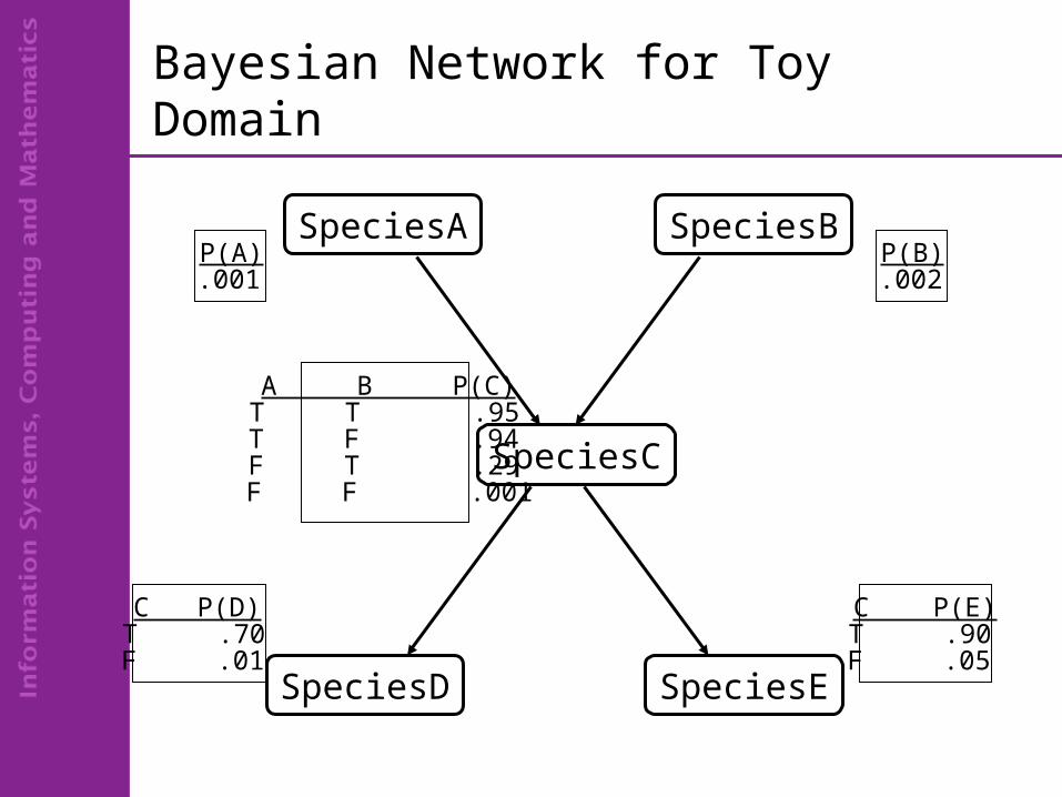
Bayesian Network for Toy DomainSpeciesCSpeciesDSpeciesEP(A)P(B).001.002A B P(C)T T .95T F .94F T .29F F .001C P(E)C P(D)T .70F .01T .90F .05SpeciesASpeciesB

Bayesian Networks Bayesian Network Demo [Species_Net] Use algorithms to learn structure and parameters from data Or build by hand (priors) Also continuous nodes (density functions)

Informative Priors To build BNs we can also use prior structures and probabilities These are then updated with data Usually uniform (equal probability) Informative Priors used to incorporate existing knowledge into BNs

Bayesian Networks for Classification & Feature Selection Node that represents the class label attached to the data

Dynamic Bayesian Networks for Forecasting

Nodes represent variables at distinct time slices Links between nodes over time Can be used to forecast into the future[Species_Dynamic_Net]

Hidden Markov ModelsLike a DBN but with hidden nodes:

Often used to model sequencesHT-1HTOT-1OT

Typical Algorithms for HMMs Given an observed sequence and a model, how do we compute its probability given the model? Given the observed sequence and the model, how do we choose an optimal hidden state sequence? How do we adjust the model parameters to maximise the probability of the observed sequence given the model?

Summary Different learning tasks can be used to solve real world problems Machine Learning techniques useful when lots of data and lots of gaps in knowledge Bayesian Networks: probabilistic framework that can perform most key ML tasks Also transparent & can incorporate expert knowledge

Some Preliminary Results on Northern Gulf DataPart 3

Expert Knowledge Ask marine biologists to generate matrices of expected relationships Can be used to compare models learnt from data Also to be used as priors to improve model quality

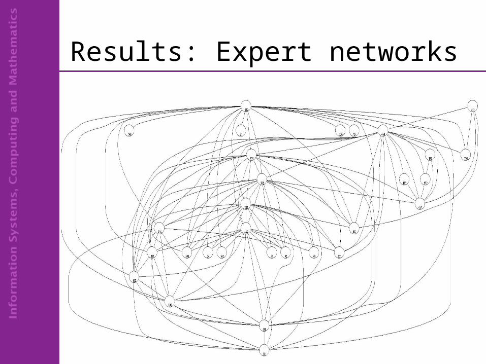
Results: Expert networks

Results: Data networks (BN from correlation) 85% conf. imputed from 70% data

Warning: data quality, spurious relationsCodHaddockWitch FlounderShrimp(Lumpfish)(Silver Hake)(Atlantic soft pout / Bristlemouths)(Eel pout / Ocean Sun Fish)

Example DBN Lets look at an example DBN [NGulfDynamic - range] Structure Encoded by knowledge Updated by data Explore with queries Supported by previous knowledge:In the Northern gulf of st. Lawrence, cod (code 438) and redfish (792,793,794,795,796) collapsed to very low levels in the mid 1990s. Subsequently the shrimp (8111) increased greatly in biomass so one will see this signal in the data. It is hypothesised that these are exclusive community states where you never get high abundance of both at the same time owing to predatory interactions.

Feature Selection Given that we know that from 1990 the cod population collapsed

Can we apply Feature Selection to see what species characterise this collapse

[Learn BN and apply CV]

Results 7: Feature Selection with BootstrapWrapper method using BNsFilter method using Log LikelihoodRedfish

Chart4

-36.5564189799

-37.3316582121

-37.5326895759

-37.9626205356

-38.0331424642

-38.3125407541

-39.9497392547

-40.4576665159

-40.5617131986

-40.6349436003

-40.8780666356

-41.3795512009

-41.5769545061

-42.1324446291

-42.2365944398

-42.3787338697

-42.5592419824

-42.5613224744

-42.5802634215

-42.586722187

-42.6207796689

-43.1770677446

-43.2347050764

-43.2993031199

-43.351442117

-43.5276588939

-44.0645779225

-44.1488270168

-44.4228045865

-44.5445747055

-44.7694816522

-44.7968659676

-44.8636211186

-44.8778249295

-44.8975067025

-44.9293756824

-45.0320310134

-45.1532559396

-45.180354309

-45.3273497095

-45.3668805595

-45.3789295849

-45.4639782337

-45.4749551049

-45.5028529795

-45.5282433626

-45.5345956723

-45.5432893369

-45.5976323711

-45.6351646581

-45.6415628655

-45.7831833953

-45.7903192138

-45.8070805423

-45.8304134011

-46.018729707

-46.1770700279

-46.2660244895

NaN

Sheet1

IDFilterLogLikIDBNWrapper

438NaN438NaN

890-36.55641897994410.76

447-37.33165821214470.7

441-37.53268957598900.34

449-37.9626205356120.32

90-38.0331424642900.3

8135-38.31254075414490.28

320-39.94973925471930.26

12-40.45766651593200.24

859-40.56171319864610.24

745-40.63494360034440.14

27-40.8780666356270.12

478-41.37955120097210.12

461-41.576954506181350.12

193-42.13244462911500.1

730-42.23659443984260.1

849-42.37873386979660.1

187-42.55924198241870.08

8217-42.56132247445720.08

8111-42.58026342157000.08

444-42.5867221877920.06

4753-42.62077966898590.06

8196-43.177067744647530.06

150-43.234705076480570.06

721-43.299303119981120.06

8213-43.3514421174430.04

844-43.52765889397010.04

24-44.06457792257170.04

443-44.14882701687450.04

966-44.422804586581380.04

451-44.544574705581960.04

792-44.769481652282170.04

426-44.7968659676240.02

726-44.86362111864780.02

700-44.87782492957260.02

809-44.89750670257300.02

9995-44.92937568248080.02

893-45.03203101348090.02

819-45.15325593968920.02

8112-45.18035430980930.02

8178-45.327349709581110.02

889-45.3668805595910

814-45.37892958494510

572-45.46397823377110

808-45.47495510497160

836-45.50285297958120

8138-45.52824336268140

711-45.53459567238190

8218-45.54328933698350

4894-45.59763237118360

701-45.63516465818440

716-45.64156286558490

892-45.78318339538890

835-45.79031921388930

812-45.807080542348940

8057-45.830413401181780

91-46.01872970782130

717-46.177070027982180

8093-46.266024489599950

Sheet1

NaN

Sheet2

NaN

Sheet3

Chart3

0.76

0.7

0.34

0.32

0.3

0.28

0.26

0.24

0.24

0.14

0.12

0.12

0.12

0.1

0.1

0.1

0.08

0.08

0.08

0.06

0.06

0.06

0.06

0.06

0.04

0.04

0.04

0.04

0.04

0.04

0.04

0.02

0.02

0.02

0.02

0.02

0.02

0.02

0.02

0.02

0

0

0

0

0

0

0

0

0

0

0

0

0

0

0

0

0

0

NaN

Sheet1

IDFilterLogLikIDBNWrapper

438NaN438NaN

890-36.55641897994410.76

447-37.33165821214470.7

441-37.53268957598900.34

449-37.9626205356120.32

90-38.0331424642900.3

8135-38.31254075414490.28

320-39.94973925471930.26

12-40.45766651593200.24

859-40.56171319864610.24

745-40.63494360034440.14

27-40.8780666356270.12

478-41.37955120097210.12

461-41.576954506181350.12

193-42.13244462911500.1

730-42.23659443984260.1

849-42.37873386979660.1

187-42.55924198241870.08

8217-42.56132247445720.08

8111-42.58026342157000.08

444-42.5867221877920.06

4753-42.62077966898590.06

8196-43.177067744647530.06

150-43.234705076480570.06

721-43.299303119981120.06

8213-43.3514421174430.04

844-43.52765889397010.04

24-44.06457792257170.04

443-44.14882701687450.04

966-44.422804586581380.04

451-44.544574705581960.04

792-44.769481652282170.04

426-44.7968659676240.02

726-44.86362111864780.02

700-44.87782492957260.02

809-44.89750670257300.02

9995-44.92937568248080.02

893-45.03203101348090.02

819-45.15325593968920.02

8112-45.18035430980930.02

8178-45.327349709581110.02

889-45.3668805595910

814-45.37892958494510

572-45.46397823377110

808-45.47495510497160

836-45.50285297958120

8138-45.52824336268140

711-45.53459567238190

8218-45.54328933698350

4894-45.59763237118360

701-45.63516465818440

716-45.64156286558490

892-45.78318339538890

835-45.79031921388930

812-45.807080542348940

8057-45.830413401181780

91-46.01872970782130

717-46.177070027982180

8093-46.266024489599950

Sheet1

NaN

Sheet2

NaN

Sheet3

Results : Feature Selection Change in Correlation of interactions between cod and high ranking species before and after 1990:

Chart2

0.37066995510.3495395732

0.14144041280.1610910182

0.1297695368-0.3051676038

0.6612700760.4350176057

-0.58003523060.3907450991

0.3528178170.0459166222

0.34551652790.6154142485

-0.35723547510.2332149257

-0.5374458998-0.1179199749

pre 1990 correlation

post 1990 correlation

Sheet1

pre 90post90pre 1990 correlationpost 1990 correlation

120.37066995510.3495395732white hake0.37066995510.349539573212white hakeUrophycis tenuis

24-0.4222590092-0.0139235787thorny skate0.14144041280.161091018290thorny skateAmblyraja radiata

27-0.2081447127-0.1057748952sea raven0.1297695368-0.3051676038320sea ravenHemitripterus americanus

900.14144041280.1610910182haddock0.6612700760.4350176057441haddockMelanogrammus aeglefinus

91-0.753221550.4009819183white hake-0.58003523060.3907450991447white hakeUrophycis tenuis

150-0.4609864394-0.1510233633silver hake0.3528178170.0459166222449silver hakeMerluccius bilinearis

1870.18084000390.1680898651witch flounder0.34551652790.6154142485890witch flounderGlyptocephalus cynoglossus

193-0.3338545374-0.344478486redfish*-0.35723547510.2332149257792

3200.1297695368-0.3051676038shrimp*-0.5374458998-0.11791997498111

426-0.6980991635-0.1338940721

4410.6612700760.4350176057

4430.2822837644-0.5644773614

444-0.23786317150.3074223492

447-0.58003523060.3907450991

4490.3528178170.0459166222

4510.6734159957-0.2742618724

461-0.28450222760.0681090425

4780.0306269028-0.2278689811

572-0.66974634430.3493657921

700-0.7383421838-0.2919316427

7010.6634773306-0.1635767821

711-0.5721417324-0.4777842184

716-0.4737570426-0.4348755415

717-0.5726933449-0.6384393546

721-0.7638557754-0.3587563312

726-0.45655618920.3196667832

7300.43787956840.0640002301

7450.57352394-0.3026726781

792-0.35723547510.2332149257

808-0.61922697580.3112109633

8090.3835075484-0.4600289539

812-0.44014455240.2901187777

814-0.2645512063-0.4094937806

8190.5089207144-0.4985525354

8350.14176096620.0496341378

836-0.4119734170.1698328398

8440.5195978596-0.1910841268

8490.33334742890.1285411531

8590.0335278698-0.0987958955

889-0.04430713170.5360750363

8900.34551652790.6154142485

8920.47558402030.0509279898

8930.4396211304-0.0680518719

966-0.2841761436-0.604453909

47530.0797362762-0.097116562

4894-0.5307580478-0.3757597184

8057-10.1861906686

80931-0.3815856512

8111-0.5374458998-0.1179199749

8112-1-0.0491881636

813510.3794762569

8138-1-0.3990574726

81780.593840903-0.1011763657

8196-0.6159174238-0.4327924872

8213-0.0408136207-0.1217855432

8217-0.6677242963-0.033252965

82180.29107542470.0654612811

9995-0.79891816010.6166102403

Sheet1

pre 1990 correlation

post 1990 correlation

Sheet2

Sheet3

Dynamic Models Given that the data is a time-series Can we build dynamic models to forecast future states? Can we use HMM to classify the time-series?

Multivariate Time Series N Gulf is process measured over time Autoregressive Correlation Function (here cod) Cross Correlation Function (here hake to cod)ACFCCF

Chart1

1

0.674

0.564

0.371

0.227

0.232

0.083

-0.013

-0.148

-0.205

-0.199

-0.219

-0.179

-0.248

Time Lag

Correlation

Sheet1

Sheet2

Sheet3

Chart1

0.071

0.216

0.244

0.463

0.683

0.686

0.791

0.561

0.46

0.392

0.317

Time Lag

Correlation

temp

CODACF

012345678910111213

10.6740.5640.3710.2270.2320.083-0.013-0.148-0.205-0.199-0.219-0.179-0.248

CODHAKECCF

-5-4-3-2-1012345

0.0710.2160.2440.4630.6830.6860.7910.5610.460.3920.317

temp

Time Lag

Correlation

Time Lag

Correlation

Results 3: Fitting Dynamic ModelsHMM Expert with CCF > 0.3 (maxlag = 5)LSS = 8.3237

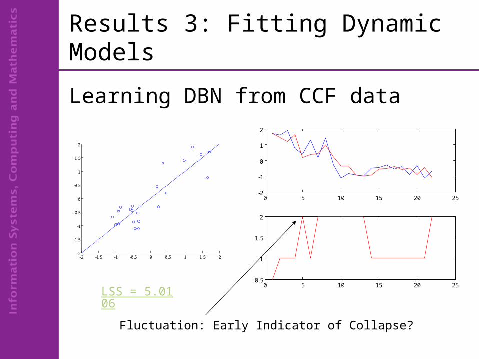
Results 3: Fitting Dynamic ModelsLearning DBN from CCF dataLSS = 5.0106Fluctuation: Early Indicator of Collapse?

Results 4: Examining DBN NetData only Dynamic Links:CodHakesHaddockWhite HakeRedfishWitch FlounderShrimpThorny Skate

Results 5: Fitting Dynamic ModelsLearning DBN from Expert biased CCF data CCF > 0.5 (maxlag=5)LSS = 6.1326

Results 6: Examining DBN NetData Biased Expert Dynamic Links:CodWitch FlounderHerringMackerel / Capelin

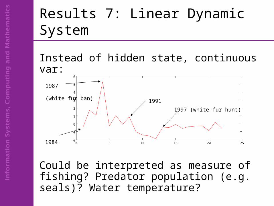
Results 7: Linear Dynamic SystemInstead of hidden state, continuous var:

Could be interpreted as measure of fishing? Predator population (e.g. seals)? Water temperature?198419911987 (white fur ban)1997 (white fur hunt)

Conclusions Hopefully conveyed the broad idea of machine learning Shown how it can be used to help analyse data like fish population data Potentially applicable to other data studied here at MLI

Potential ProjectsSpatio-Temporal AnalysisUse Spatio-Temporal BNs to model fish stock data. Nodes would represent species in specific regionsCombining Expert Knowledge and Data for improved PredictionLooking for Un/Stable States and the factors that influence themFunctional Analysis of Data from Multiple Locations

E.G. Spatial Analysis Spatial Bayesian Network Analysis [NGulfCodSpatial]

E.G. Functional Models Functional Models to assimilate data from different oceans...

Acknowledgements:

Daniel DupliseaPanayiota Apostolaki

Any Questions?

************************************************