machine teaching - tu darmstadt publication...
TRANSCRIPT

Machine TeachingA Machine Learning Approach to Technology Enhanced Learning
Dissertation
Zur Erlangung des akademischen Gradeseines Doktor-Ingenieur (Dr.-Ing.)
Eingereicht vonDiplom Wirtschaftsinformatiker Markus Weimergeb. in Hadamar
Angenommen vom Fachbereich Informatikder Technischen Universitat Darmstadt
Gutachter: Prof. Dr. Max Muhlhauser (TU Darmstadt)
Prof. Dr. Alexander J. SmolaAustralian National University, Canberra, AustralienYahoo! Research, Santa Clara, CA, USA
Prof. Dr. Petra Gehring (TU Darmstadt)
Tag der Einreichung: 14.07.2009Tag der Disputation: 24.09.2009
Darmstadter Dissertationen, D17 Erschienen in 2010 in Darmstadt.

Abstract
Many applications of Technology Enhanced Learning are based on strong assump-tions: Knowledge needs to be standardized, structured and most of all externalizedinto learning material that preferably is annotated with meta-data for efficient re-use.A vast body of valuable knowledge does not meet these assumptions, including infor-mal knowledge such as experience and intuition that is key to many complex activities.
We notice that knowledge, even if not standardized, structured and externalized, canstill be observed through its application. We refer to this observable knowledge as PRAC-TICED KNOWLEDGE. We propose a novel approach to Technology Enhanced Learningnamed MACHINE TEACHING to convey this knowledge: Machine Learning techniquesare used to extract machine models of Practiced Knowledge from observational data.These models are then applied in the learner’s context for his support.
We identify two important subclasses of machine teaching, General and DetailedFeedback Machine Teaching. GENERAL FEEDBACK MACHINE TEACHING aims to pro-vide the learner with a “grade-like” numerical rating of his work. This is a direct ap-plication of supervised machine learning approaches. DETAILED FEEDBACK MACHINE
TEACHING aims to provide the learner with in-depth support with respect to his activ-ities. An analysis showed that a large subclass of Detailed Feedback Machine Teachingapplications can be addressed through adapted recommender systems technology.
The ability of the underlying machine learning techniques to capture structure andpatterns in the observational data is crucial to the overall applicability of MachineTeaching. Therefore, we study the feasibility of Machine Teaching from a machinelearning perspective.
Following this goal, we evaluate the General Feedback Machine Teaching approachusing state-of-the-art machine learning techniques: The exemplary Machine Teachingsystem is sought to provide the learner with quality estimations of his writing as judgedby an online community. The results obtained in this evaluation are supportive of theapplicability of Machine Teaching to this domain.
To facilitate Detailed Feedback Machine Teaching, we present a novel matrix factor-ization model and algorithm. In addition to addressing the needs of Machine Teaching,it is also a contribution to the recommender systems field as it facilitates ranking esti-mation. An Evaluation in a Detailed Feedback Machine Teaching scenario for softwareengineers supports the feasibility of Machine Teaching in that domain.
We therefore conclude that machine learning models capable of capturing importantaspects of practiced knowledge can be found in both, General and Detailed FeedbackMachine Teaching. Machine Teaching does not assume the knowledge to be external-ized, but to be observable and therefore adds another body of knowledge to Technol-ogy Enhanced Learning not amenable to traditional Technology Enhanced Learningapproaches.
3

4

Zusammenfassung
Viele erfolgreiche E-Learning Systeme basieren auf strengen Annahmen: Das zu vermit-telnde Wissen muss strukturiert und standardisiert in Lerninhalte externalisiert sein.Diese wiederum sollten mit Metadaten angereichert sein, um ihre Wiederverwendungzu ermoglichen. Diese strikten Anforderungen verhindern es, fur viele Aktivitaten ent-scheidendes informelles Wissen, also unter anderem Erfahrung und Intuition, zu ver-mitteln.
Wissen, auch wenn es weder standardisiert, strukturiert noch externalisiert wurde,manifestiert sich in Aktivitaten seiner Trager. Wir nennen dieses beobachtbare WissenPRAKTIZIERTES WISSEN. In dieser Dissertation wird MACHINE TEACHING eingefuhrt,ein neuer Ansatz zum E-Learning, der diese Tatsache wie folgt ausnutzt: Aus Beobach-tungsdaten werden mit Methoden des maschinellen Lernens Modelle extrahiert, diedann im Kontext des Lerners zu seiner Unterstutzung eingesetzt werden.
Innerhalb dieses Ansatzes werden zwei wichtige Teilaufgaben eines Machine Tea-ching Systems identifiziert: Generelles und Detailliertes Feedback. Ziel von MachineTeaching fur Generelles Feedback ist es, die Arbeit des Lerners zu bewerten, etwa durch,,Zensuren”. Dies kann durch aktuelle Verfahren des uberwachten maschinellen Lernengeleistet werden. Machine Teaching fur Detailliertes Feedback soll den Lerner hinge-gen mit feingranularen Hinweisen zu seiner Arbeit unterstutzen. Wir zeigen, dass eingroßer Anteil dieser Aufgabe mittels angepasster Recommender Systems Technologiebearbeitet werden kann.
Die Nutzlichkeit zukunftiger Machine Teaching Systeme wird vor allem davon ab-hangen, wie gut es mittels maschineller Lernverfahren moglich ist, das Praktizierte Wis-sen in Form von Mustern und Strukturen aus den Beobachtungsdaten zu extrahieren.Folglich wird in dieser Dissertation untersucht, ob und in wie weit dies moglich ist.
Die erste Evaluation hierzu erfolgt am Beispiel eines Machine Teaching Systems furgenerelles Feedback. Es wird ein System evaluiert, das Texte automatisch bewertet.Dies geschieht auf Basis vergangener Bewertungen anderer Texte durch eine InternetCommunity. Aus der Leistung des Systems bei dieser Aufgabe folgt, dass Machine Te-aching fur generelles Feedback hier erfolgreich eingesetzt werden kann.
Um Machine Teaching fur detailliertes Feedback zu ermoglichen, stellen wir ein neu-es Modell fur Recommender Systeme vor. Dieses Modell stellt eine Erweiterung desMatrixfaktorisierungsansatzes dar. Neben seiner Ausrichtung auf Machine Teachingist der Algorithmus der erste, der Reihenfolgevorhersagen fur Recommender Syste-me ermoglicht. Wir evaluieren ihn in einem Machine Teaching Ansatz fur detaillier-tes Feedback im Bereich Softwareentwicklung. Basierend auf einer Quelltextdatenbanksoll dieser auf fehlende Aufrufe hinweisen. Auch hier lassen die empirischen Ergebnis-se schliessen, dass Machine Teaching in dieser Domane anwendbar ist.
Machine Teaching stellt also eine machbare Erweiterung des E-Learning dar, dessenEinsatzbreite mit dem Fortschritt des maschinellen Lernens wachst. Es erweitert bishe-rige Ansatze um beobachtbares und damit eben auch informelles Wissen, das bisher imE-Learning nur schwer vermittelbar ist.
5

Acknowledgements
This work would not have been possible without the support and encouragement ofmy advisors, colleagues and fellow PhD students. I am grateful to all those who con-tributed to the outcome of this thesis.
First and foremost, I would like to thank my advisors Max Muhlhauser (TU Darm-stadt) and Alex Smola (Australian National University, Yahoo! Research). They sup-ported me with sharing their respective expertise in Technology Enhanced Learningand Machine Learning, but even more so with excellent advice on research in general.
My work in the past three years has been defined by fruitful and intense collabora-tions: The most influential has been with Alexandros Karatzoglou who I worked withas if he shared an office with me, despite the fact that he held several different positionsat TU Vienna (Austria), CIRO (Sydney, Australia) and INRIA (Rouen, France) duringour collaboration. I am also thankful for the collaboration with and advice from MarcelBruch(TU Darmstadt) and Quoc Viet Le (Stanford University), Choon-Hui Theo (Aus-tralian National University) and my colleagues at NICTA (Canberra, Australia) andYahoo! Research (Santa Clara, California) during my respective visits.
I am grateful for having been a member of the interdisciplinary postgraduate school“eLearning” at TU Darmstadt, the context in which my work was funded. I thank alladvisors and all Ph.D. students of the postgraduate school for providing an inspiringatmosphere and hosting cross-disciplinary discussions. In particular, Andreas Kamin-ski and Petra Gehring have been of tremendous help in sharpening many of the argu-ments in the present thesis by asking the right, tough questions before and in the reviewprocess.
Many thanks are due to all present and former members of the Telecooperation groupat TU Darmstadt. They provided a very friendly place to work and supported thisthesis in many respects. I am also grateful for the support by the Frankfurt Center forScientific Computing in running many of the experiments reported in this thesis.
Last but not least, I am very grateful to my family which always supported me.
7


Contents
1 Introduction 171.1 Motivation: The need for Machine Teaching . . . . . . . . . . . . . . . . . 181.2 Approach taken . . . . . . . . . . . . . . . . . . . . . . . . . . . . . . . . . 211.3 Organization of this Thesis . . . . . . . . . . . . . . . . . . . . . . . . . . . 221.4 Contributions of this Thesis . . . . . . . . . . . . . . . . . . . . . . . . . . 23
2 The Machine Teaching Approach 272.1 Preliminaries: A Brief Introduction to Machine Learning . . . . . . . . . 28
2.1.1 Machine Learning Problems . . . . . . . . . . . . . . . . . . . . . . 282.1.2 Machine Learning Models . . . . . . . . . . . . . . . . . . . . . . . 302.1.3 Machine Learning Methods . . . . . . . . . . . . . . . . . . . . . . 312.1.4 The Kernel Trick . . . . . . . . . . . . . . . . . . . . . . . . . . . . 34
2.2 Introducing Machine Teaching . . . . . . . . . . . . . . . . . . . . . . . . 352.2.1 Definition . . . . . . . . . . . . . . . . . . . . . . . . . . . . . . . . 352.2.2 High-Level Example of a Machine Teaching Scenario . . . . . . . 372.2.3 Machine Teaching Properties . . . . . . . . . . . . . . . . . . . . . 372.2.4 Machine Teaching Assumptions . . . . . . . . . . . . . . . . . . . 39
2.3 Major Components of a Machine Teaching System . . . . . . . . . . . . . 392.3.1 Dynamics of a Machine Teaching System . . . . . . . . . . . . . . 422.3.2 Focus of this Thesis . . . . . . . . . . . . . . . . . . . . . . . . . . . 44
2.4 General Feedback Machine Teaching . . . . . . . . . . . . . . . . . . . . . 452.5 Detailed Feedback Machine Teaching . . . . . . . . . . . . . . . . . . . . 472.6 Conclusion . . . . . . . . . . . . . . . . . . . . . . . . . . . . . . . . . . . . 51
3 General Feedback Machine Teaching for Web Forum Authors 533.1 Introduction . . . . . . . . . . . . . . . . . . . . . . . . . . . . . . . . . . . 54
3.1.1 Example domain . . . . . . . . . . . . . . . . . . . . . . . . . . . . 543.2 State of the Art . . . . . . . . . . . . . . . . . . . . . . . . . . . . . . . . . . 55
3.2.1 Automatic Essay Scoring . . . . . . . . . . . . . . . . . . . . . . . 563.2.2 Data Characteristics . . . . . . . . . . . . . . . . . . . . . . . . . . 563.2.3 Feature Inspirations . . . . . . . . . . . . . . . . . . . . . . . . . . 56
3.3 Feature Engineering . . . . . . . . . . . . . . . . . . . . . . . . . . . . . . 573.3.1 Surface Features . . . . . . . . . . . . . . . . . . . . . . . . . . . . 583.3.2 Lexical Features . . . . . . . . . . . . . . . . . . . . . . . . . . . . . 583.3.3 Syntactic Features . . . . . . . . . . . . . . . . . . . . . . . . . . . . 593.3.4 Forum Specific Features . . . . . . . . . . . . . . . . . . . . . . . . 59
9

Contents
3.3.5 Similarity features . . . . . . . . . . . . . . . . . . . . . . . . . . . 593.4 Evaluation Procedure . . . . . . . . . . . . . . . . . . . . . . . . . . . . . . 60
3.4.1 Data Set and Pre-processing . . . . . . . . . . . . . . . . . . . . . . 603.4.2 Method . . . . . . . . . . . . . . . . . . . . . . . . . . . . . . . . . . 61
3.5 Evaluation Results and Discussion . . . . . . . . . . . . . . . . . . . . . . 623.5.1 Results . . . . . . . . . . . . . . . . . . . . . . . . . . . . . . . . . . 623.5.2 Performance Analysis . . . . . . . . . . . . . . . . . . . . . . . . . 63
3.6 Conclusion . . . . . . . . . . . . . . . . . . . . . . . . . . . . . . . . . . . . 68
4 Generalized Matrix Factorization 694.1 Introduction . . . . . . . . . . . . . . . . . . . . . . . . . . . . . . . . . . . 704.2 State of the Art . . . . . . . . . . . . . . . . . . . . . . . . . . . . . . . . . . 714.3 Regularized Matrix Factorization . . . . . . . . . . . . . . . . . . . . . . . 734.4 Loss Functions . . . . . . . . . . . . . . . . . . . . . . . . . . . . . . . . . . 76
4.4.1 Element Based Loss Functions . . . . . . . . . . . . . . . . . . . . 764.4.2 Row Based Loss Functions . . . . . . . . . . . . . . . . . . . . . . 794.4.3 A faster Ordinal Regression Loss Function . . . . . . . . . . . . . 804.4.4 An NDCG Loss Function for Matrix Factorization . . . . . . . . . 854.4.5 Conclusion . . . . . . . . . . . . . . . . . . . . . . . . . . . . . . . 92
4.5 Optimization . . . . . . . . . . . . . . . . . . . . . . . . . . . . . . . . . . . 924.5.1 Optimization over the Row Matrix R . . . . . . . . . . . . . . . . 954.5.2 Optimization over the Row Matrix C . . . . . . . . . . . . . . . . 954.5.3 New Row Optimization . . . . . . . . . . . . . . . . . . . . . . . . 96
4.6 Extensions to the Regularized Matrix Factorization Model . . . . . . . . 964.6.1 Row and Column Biases . . . . . . . . . . . . . . . . . . . . . . . . 964.6.2 Adaptive Regularization . . . . . . . . . . . . . . . . . . . . . . . . 974.6.3 Structure Exploitation with a Graph Kernel . . . . . . . . . . . . . 984.6.4 Row and Column Features . . . . . . . . . . . . . . . . . . . . . . 98
4.7 Conclusion . . . . . . . . . . . . . . . . . . . . . . . . . . . . . . . . . . . . 99
5 Evaluation on Recommender Systems Data 1015.1 Evaluation Setup . . . . . . . . . . . . . . . . . . . . . . . . . . . . . . . . 102
5.1.1 Evaluation Measures . . . . . . . . . . . . . . . . . . . . . . . . . . 1025.1.2 Evaluation Procedure . . . . . . . . . . . . . . . . . . . . . . . . . 1035.1.3 Data Sets . . . . . . . . . . . . . . . . . . . . . . . . . . . . . . . . . 104
5.2 Results and Discussion . . . . . . . . . . . . . . . . . . . . . . . . . . . . . 1055.2.1 Model Extensions . . . . . . . . . . . . . . . . . . . . . . . . . . . . 1055.2.2 Ranking Losses . . . . . . . . . . . . . . . . . . . . . . . . . . . . . 106
5.3 Conclusion . . . . . . . . . . . . . . . . . . . . . . . . . . . . . . . . . . . . 109
6 Detailed Feedback Machine Teaching for Software Engineers 1116.1 Introduction . . . . . . . . . . . . . . . . . . . . . . . . . . . . . . . . . . . 112
6.1.1 Application Domain: Programming with Frameworks . . . . . . 1126.2 Related Work . . . . . . . . . . . . . . . . . . . . . . . . . . . . . . . . . . 114
10

Contents
6.3 Matrix Factorization Modeling . . . . . . . . . . . . . . . . . . . . . . . . 1166.4 Evaluation Setup . . . . . . . . . . . . . . . . . . . . . . . . . . . . . . . . 116
6.4.1 Method . . . . . . . . . . . . . . . . . . . . . . . . . . . . . . . . . . 1176.4.2 Data Set . . . . . . . . . . . . . . . . . . . . . . . . . . . . . . . . . 1186.4.3 Baseline System . . . . . . . . . . . . . . . . . . . . . . . . . . . . . 120
6.5 Evaluation Results and Discussion . . . . . . . . . . . . . . . . . . . . . . 1216.6 Conclusion . . . . . . . . . . . . . . . . . . . . . . . . . . . . . . . . . . . . 126
7 Conclusions 1297.1 Summary . . . . . . . . . . . . . . . . . . . . . . . . . . . . . . . . . . . . . 1307.2 Future Work . . . . . . . . . . . . . . . . . . . . . . . . . . . . . . . . . . . 132
Bibliography 139
11


List of Algorithms
1 Ordinal Regression in O(m2) . . . . . . . . . . . . . . . . . . . . . . . . . 82
2 Ordinal Regression in O (m log m) . . . . . . . . . . . . . . . . . . . . . . 843 Alternate Subspace Descent for Matrix Factorization . . . . . . . . . . . . 934 Optimization over R with fixed C . . . . . . . . . . . . . . . . . . . . . . . 955 Efficient computation of ∂CL . . . . . . . . . . . . . . . . . . . . . . . . . . 96
13


List of Figures
1.1 Visualization of Machine Teaching as an alternative to the traditionaltechnology enhanced learning approach. . . . . . . . . . . . . . . . . . . 21
1.2 Structure of this thesis . . . . . . . . . . . . . . . . . . . . . . . . . . . . . 22
2.1 Underfitting . . . . . . . . . . . . . . . . . . . . . . . . . . . . . . . . . . . 322.2 Overfitting . . . . . . . . . . . . . . . . . . . . . . . . . . . . . . . . . . . . 332.3 Major components of a Machine Teaching system . . . . . . . . . . . . . 402.4 Mockup of the user interface of a Machine Teaching System for program-
mers. . . . . . . . . . . . . . . . . . . . . . . . . . . . . . . . . . . . . . . . 42
4.1 Machine Teaching and Recommender System data as a matrix . . . . . . 714.2 The fast procedure to compute the ordinal regression loss. . . . . . . . . 834.3 Visualization of the sensitivity of DCG to different errors . . . . . . . . . 864.4 A convex function (solid) is bounded from below by Taylor approxima-
tions of first order (dashed). Adding more terms improves the bound. . 94
6.1 Mockup of the user interface of a Detailed Feedback Machine Teachingsystem for software engineers. . . . . . . . . . . . . . . . . . . . . . . . . 113
6.2 Representing call relations in source code as a sparse matrix when usingclasses as the context. . . . . . . . . . . . . . . . . . . . . . . . . . . . . . . 117
6.3 Histogram of the number of calls to SWT per class in Eclipse . . . . . . . 1196.4 Histogram of the number of calls per SWT method . . . . . . . . . . . . . 1206.5 F1, precision and recall results for the Method and Class data for the rule
based approach and matrix factorization using the soft margin and theregression loss functions. . . . . . . . . . . . . . . . . . . . . . . . . . . . . 122
6.6 F1, precision and recall for the matrix factorization system with a softmargin loss for different value of the weight parameter (on a natural logscale) . . . . . . . . . . . . . . . . . . . . . . . . . . . . . . . . . . . . . . . 124
6.7 Results for F1, precision and recall obtained with the matrix factorizationsystem with a soft margin loss and different values for the number offactors parameter . . . . . . . . . . . . . . . . . . . . . . . . . . . . . . . . 125
15


1 Introduction
Contents1.1 Motivation: The need for Machine Teaching . . . . . . . . . . . . . . . 181.2 Approach taken . . . . . . . . . . . . . . . . . . . . . . . . . . . . . . . . 211.3 Organization of this Thesis . . . . . . . . . . . . . . . . . . . . . . . . . 221.4 Contributions of this Thesis . . . . . . . . . . . . . . . . . . . . . . . . 23
17

1 Introduction
1.1 Motivation: The need for Machine Teaching
Today, Technology Enhanced Learning is applied in many instances. Most commonlyknown to students are Learning Management Systems (LMS). A learning managementsystem is used to support the processes in a formal learning setting such as withinuniversities by providing means for content distribution, communication and collabo-ration. Well known examples include the open source packages Moodle [Com09a] andSakai [Com09b] as well as commercial products, e.g. the Blackboard system [Bla09]used by universities worldwide.
Tools like Power Trainer [QABC09] and Lecturnity [AG09] support the teachers increating the content to be made available through the learning management systems.There are even mature content standards such as the Sharable Content Object ReferenceModel (SCORM) [Lea09] and the ones set by the IMS Global Learning Consortium1.These standards facilitate the use of sophisticated meta-data schemes that describe thecontent to support the mix-and-match of content from different authors.
Adaptive hypermedia approaches such as AHA! [DBSS06] build upon these systemsand standards to allow the teacher to build adaptive content by expressing rules like“To understand concept X, the student shall know concept A, B and C”. These rules arethen used to support the student’s navigation in the content.
Despite these successful applications of technology enhanced learning, there is agrowing interest in what is called “eLearning 2.0” to overcome the inherent limits ofthe dominant approaches to technology enhanced learning, including those mentionedso far. This thesis contributes to this movement by introducing a machine learningbased approach to technology enhanced learning.
Before presenting a critique of the traditional technology enhanced learning approa-ches, we introduce the following notation:
Notation 1 (Learner). We use the term “learner” throughout this thesis deliberately insteadof “student”, as the proposed approach is primarily aimed at informal learning and not limitedto formal learning scenarios like those found in university courses.
Assumptions of Traditional Technology Enhanced Learning
The approach presented in this thesis departs from traditional technology enhancedlearning by overcoming certain limiting assumptions regarding the knowledge and thelearners which shall be argued below:
Assumptions with respect to Knowledge
We argue that knowledge in traditional technology enhanced learning approaches isassumed to be standardized, externalized and structured: Content authoring for tech-nology enhanced learning is costly. Thus, there is a focus on standardized knowledgethat applies to a wide audience. By its very definition, technology enhanced learning
1http://www.imsglobal.org
18

1.1 Motivation: The need for Machine Teaching
enforces the knowledge to be externalized into content, also frequently called learningmaterial, e. g. in the form of web based training material.
Lastly, one can observe a tendency towards structured knowledge or representationsthereof. Standards like the aforementioned SCORM [Lea09] represent the spearhead ofthis movement: They facilitate the exchange of learning materials between courses bystandardizing meta data regarding the sequence of that material.
(Slightly) Exaggerated Conclusion: If one follows this line of thought to the extreme,content and therefore knowledge is treated like source code to facilitate automated pro-cesses upon this content such as re-purposing content from one course to another. Themeta-data to support these processes is to be created by the content authors in additionto the content itself.
Assumptions with respect to Learners
Following their focus on formal learning settings, e. g. in higher education, traditionaltechnology enhanced learning approaches frequently assume the learner to be a stu-dent. Students can be assumed to be motivated to learn and to be focused on learningwithout distraction.
Following this strong assumption, elaborate models from cognitive science have beenapplied to model and even predict the student’s behavior as he uses the technology en-hanced learning system. One example is the cognitive architecture ACT-R that has beenapplied to technology enhanced learning as described e. g. in [AG01] and [LMA87]. Theuse of a cognitive architecture allows a system following these approaches to model thecognition of the learner from his interaction with the system.
(Slightly) Exaggerated Conclusion: If one follows this line of thinking to the extreme,the learner is thought of as a computer, whose behavior can be modeled and thereforepredicted by a technology enhanced learning system.
Challenging the Assumptions
These assumptions regarding the content and learner in a technology enhanced learn-ing scenario are far from unexpected: In fact, their prevalence follows best practicesin computer science, where each of its application domains is typically modeled in asimilar manner to the one described above to facilitate its handling through comput-ers. However, the aforementioned assumptions are not always met in many instanceswhere technology enhanced learning could be applied.
First and foremost, not all knowledge can be standardized, nor can it always be exter-nalized in a structured way. The prime example is implicit knowledge such as experience,intuition and “know-how”. Many activities are based upon implicit knowledge in ad-dition to explicit knowledge. In an informal way, explicit knowledge can be defined astextbook, formal, objective or standardized knowledge. Implicit knowledge, on theother hand, is subjective, vague and informal.
19

1 Introduction
Consider the following examples of activities where implicit knowledge is an impor-tant aspect:
Example 1 (Cases of Implicit Knowledge).
Bike Riding: Studying the physics of a bike is not sufficient to be able to successfully ride one.
Programming: Programming can only be taught to some extend explicitly through books anduniversity courses. An important aspect in programming is the experience and intuitionof the programmer. Additionally, the question of what “elegant code” exactly is, willprobably never be answered in an explicit form.
Game Play: The rules for games can be spelled out in great detail and very explicitly. How-ever, the skills of winning the game are inherently hard to convey explicitly. Instead, thisknowledge is built by making experiences with the game.
In addition to implicit knowledge that is impossible to externalize in a standardized,structured way, that process is hard or undesirable in other instances for the followingreasons:
Externalizations are costly: Externalizing knowledge is a time consuming and there-fore expensive process. Thus, it is frequently omitted for knowledge that is notneeded in a similar fashion by a large audience.
Externalizations are easily outdated If the knowledge changes quickly, its externaliza-tions are frequently outdated. Constant updates of the externalizations only addto the cost of creating and maintaining them.
The second assumptions of the learner being a student restricts technology enhancedlearning approaches to formal, explicit learning scenarios such as courses in highereducation institutions. This restriction excludes important aspects of life long learning,most importantly learning-while-doing.
However, the implicit and hard to externalize knowledge is typically transferred inlearning-while-doing scenarios in traditional learning, namely through the apprentice-ship. Thus, the exclusion of this knowledge from traditional technology enhancedlearning and an its assumptions about the learner being as student as opposed to anapprentice are congruent.
Therefore, we define the following problem to be discussed in this thesis:Problem Statement: The field of technology enhanced learning is faced witha large body of important and valuable knowledge that is not amenable to thecurrent technology enhanced learning methodology as it is not externalized in away suitable to traditional approaches in the field.
20
1.2 Approach taken
Authoring
Author
Consume
Learner
Traditional technology Enhanced Learning
Machine Teaching
Learner
Support
Machine LearningModels
Observation
Practicioners
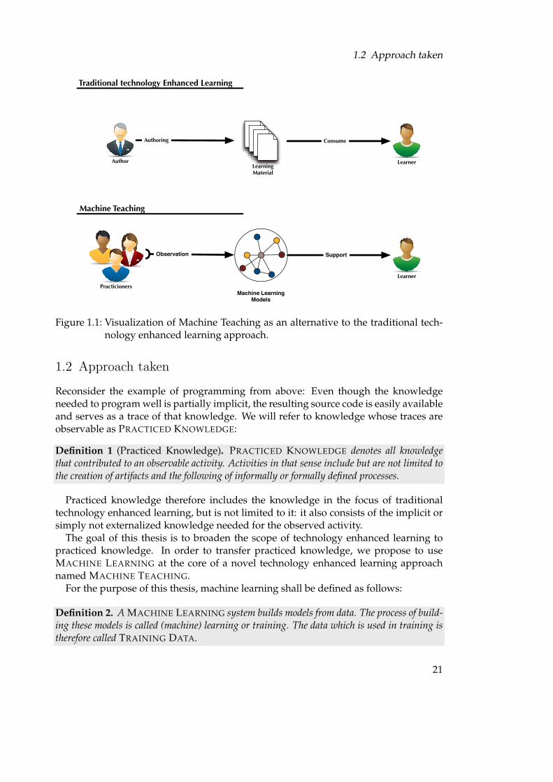
LearningMaterial
Figure 1.1: Visualization of Machine Teaching as an alternative to the traditional tech-nology enhanced learning approach.
1.2 Approach taken
Reconsider the example of programming from above: Even though the knowledgeneeded to program well is partially implicit, the resulting source code is easily availableand serves as a trace of that knowledge. We will refer to knowledge whose traces areobservable as PRACTICED KNOWLEDGE:
Definition 1 (Practiced Knowledge). PRACTICED KNOWLEDGE denotes all knowledgethat contributed to an observable activity. Activities in that sense include but are not limited tothe creation of artifacts and the following of informally or formally defined processes.
Practiced knowledge therefore includes the knowledge in the focus of traditionaltechnology enhanced learning, but is not limited to it: it also consists of the implicit orsimply not externalized knowledge needed for the observed activity.
The goal of this thesis is to broaden the scope of technology enhanced learning topracticed knowledge. In order to transfer practiced knowledge, we propose to useMACHINE LEARNING at the core of a novel technology enhanced learning approachnamed MACHINE TEACHING.
For the purpose of this thesis, machine learning shall be defined as follows:
Definition 2. A MACHINE LEARNING system builds models from data. The process of build-ing these models is called (machine) learning or training. The data which is used in training istherefore called TRAINING DATA.
21

1 Introduction
Chapter 1: Motivation
Chapter 2: Introduction and Analysis of the Machine Teaching approach
Chapter 3General Feedback Machine Teaching for
Web Forums
Chapter 4A Matrix Factorization based Algorithm for
Machine Teaching
Chapter 5Evaluation on Recommender Systems Data
Chapter 6Detailed Feedback Machine Teaching for
Software Engineers
Chapter 7: Conclusions and Future Research
Figure 1.2: Structure of this thesis
The key idea of our approach is to use the observations of successful activities as thetraining data of machine learning systems. Therefore, a model is built that capturesthe structure of these observations. This model is then brought into the context of thelearner to retrieve feedback, suggestions or general support from it.
One way of visualizing the relationship between traditional technology enhancedlearning approaches and Machine Teaching is depicted in Figure 1.1: Where traditionaltechnology enhanced learning presents the learner (student) learning material authoredfor this purpose, Machine Teaching resorts to automatically learned models build fromdata about the activity of practitioners.
Research Question: We hypothesize that machine learning models are capableof thereby transferring practiced knowledge. The validity of this hypothesisshall be the topic of this thesis.
1.3 Organization of this Thesis
Figure 1.2 visualizes the structure of this thesis. Chapter 2 introduces the MachineTeaching approach to technology Enhanced Learning more formally, after a brief intro-duction to machine learning.
The definition of the approach is followed by an theoretical analysis of its properties
22

1.4 Contributions of this Thesis
and possible applications in the same chapter. An analysis of the major components ofa hypothetical technology enhanced learning system following this approach is used toidentify research results needed in order to facilitate the realization of such a system:
Sensors that allow the Machine Teaching system to monitor both the learners and ex-perts.
Machine Learning Models capable of capturing the knowledge from the sensor data inorder to provide the learner with meaningful feedback.
For the purpose of this thesis, the sensors are tied to the artifacts created by the learn-ers and experts alike. The remainder of the thesis thus focuses on investigating anddeveloping machine learning models for Machine Teaching.
Machine Learning for Machine Teaching
The first step in this study is presented in Chapter 3, where a system is presented thatsupports the learner with automated ratings of her web forum posts. These ratings arecomputed based upon a machine learning model built from web forum posts that havebeen rated by the users of that web forum. From a machine learning perspective, sucha system is built using state-of-the-art supervised machine learning methods.
The good results of machine learning on that task encourage the analysis performedin the Chapters 4, 5 and 6 where detailed feedback in Machine Teaching is investigated.There, the goal is to support the learner with feedback regarding her artifact instead ofmerely rating it.
Chapter 4 presents a novel matrix factorization based machine learning model and al-gorithm equally suited for this task and the more broadly known task of RecommenderSystems. The algorithm is evaluated in Chapter 5 on data sets from the recommendersystems literature with promising results.
In Chapter 6, this model and algorithm are applied to build a Detailed Feedback Ma-chine Teaching approach for software engineers. Empirical evaluations show that thesystem is indeed capable of supporting a software engineer with meaningful sugges-tions.
Based on results presented in Chapter 6 and Chapter 3 it is safe to conclude thatmachine learning can in fact be used to build Machine Teaching systems.
1.4 Contributions of this Thesis
This thesis investigates using machine learning to help convey implicit knowledge. Itthereby makes the following contributions to the state of the art in machine learningand technology enhanced learning.
23

1 Introduction
Scientific Contributions
Machine Teaching Approach: This thesis presents a novel approach to technology en-hanced learning that facilitates the transfer of implicit knowledge. The approachtakes into account different scenarios of general and detailed learner feedback.
Automatic Quality Assessment of Text: The ability to write appropriately for a com-munity is a skill that cannot be transferred to explicit knowledge and thus is notamenable to the traditional technology enhanced learning methodology. How-ever, it is shown that the quality judgment of a community can be replicated bya machine in order to facilitate the self-learning of this skill. This work has beenpublished in [WG07] and [WGM07]; the feature extraction software developed aspart of this has been described in [GMM+07].
A generalized Matrix Factorization Method: Many instances of the Machine Teachingapproach can be encoded into matrix factorization problems, much like recom-mender systems. Where the latter suggest items to users, the former suggest ac-tions to take or attributes of artifacts to be created. This thesis introduces a newmodel and algorithm for this task and makes the following contributions to thisfield:
1. A generalization of matrix factorization models to per-row loss functionsand
2. an optimization procedure to do so efficiently.
3. A procedure for the direct optimization of the Normalized Discounted Cu-mulative Gain (NDCG) ranking score.
4. An algorithm for the computation of the ordinal regression loss inO (n log n)time as opposed to the algorithms of O
(n2) time complexity that have been
previously known in the literature.
5. An extension of the matrix factorization approach to hybrid recommendersthat can use features in addition to the user-item interaction data used incollaborative filtering recommender systems.
6. Adaptive regularization for matrix factorization.
7. The integration of a graph kernel to model the binary interaction e.g. be-tween users and movies in addition to the ratings provided by the users.
The algorithm has been evaluated on recommender systems data with favorableresults. The model, algorithm and extensions have been published in [WKLS08],[WKS08b], [WKS08c] and [WKS08a]. The first version of the system with theNDCG loss function was presented at NIPS 2007 under the name CofiRank inthe paper [WKLS08]. It was the first collaborative filtering system capable of pre-dicting rankings as opposed to ratings and will be presented in the PreferenceLearning book [KW10]. The recent paper [WKB09] at the ACM Recommender
24

1.4 Contributions of this Thesis
Systems Conference presents the results of the application of the Machine Teach-ing approach to the software development domain.
A machine teaching approach for programming: Learning to program with a new codelibrary is a challenging task for software developers. It is shown that a code rec-ommender system can be built for this task based on the matrix factorization al-gorithm introduced above that is capable of easing this process.
Data and Software Contributions
During this thesis, the following additional contributions have been made to the scien-tific community:
Software: An implementation of the matrix factorization algorithm in C++ has beenfound to be one of the fastest available. It has been released as Open SourceSoftware and is available from the project website http://cofirank.org fordownload.
Data Sets: Most of the experiments reported in this thesis were conducted on publiclyavailable data sets. Following this example, the data set used for the evaluationin the software engineering application has been released on the project website,too. The data set is described in detail in Section 6.4 and consists of caller-calleerelations mined from the Eclipse source code calling the SWT user interface frame-work.
25

2 The Machine Teaching Approach
Contents2.1 Preliminaries: A Brief Introduction to Machine Learning . . . . . . . 28
2.1.1 Machine Learning Problems . . . . . . . . . . . . . . . . . . . . . 282.1.2 Machine Learning Models . . . . . . . . . . . . . . . . . . . . . . 302.1.3 Machine Learning Methods . . . . . . . . . . . . . . . . . . . . . 312.1.4 The Kernel Trick . . . . . . . . . . . . . . . . . . . . . . . . . . . 34
2.2 Introducing Machine Teaching . . . . . . . . . . . . . . . . . . . . . . . 352.2.1 Definition . . . . . . . . . . . . . . . . . . . . . . . . . . . . . . . 352.2.2 High-Level Example of a Machine Teaching Scenario . . . . . . 372.2.3 Machine Teaching Properties . . . . . . . . . . . . . . . . . . . . 372.2.4 Machine Teaching Assumptions . . . . . . . . . . . . . . . . . . 39
2.3 Major Components of a Machine Teaching System . . . . . . . . . . 392.3.1 Dynamics of a Machine Teaching System . . . . . . . . . . . . . 422.3.2 Focus of this Thesis . . . . . . . . . . . . . . . . . . . . . . . . . . 44
2.4 General Feedback Machine Teaching . . . . . . . . . . . . . . . . . . . 452.5 Detailed Feedback Machine Teaching . . . . . . . . . . . . . . . . . . . 472.6 Conclusion . . . . . . . . . . . . . . . . . . . . . . . . . . . . . . . . . . 51
27

2 The Machine Teaching Approach
The goal of this chapter is two-fold: First, MACHINE TEACHING is introduced as anew technology enhanced learning approach which emphasizes on conveying prac-ticed knowledge. Second, this chapter also presents the research focus of this thesiswithin the broader approach of Machine Teaching.
The chapter is therefore structured as follows: Machine Learning is introduced in Sec-tion 2.1 to facilitate the discussion in subsequent sections. Machine Teaching is then for-mally defined and its properties are analyzed based upon that definition in Section 2.2.The major components of a Machine Teaching system are described in Section 2.3, in-cluding the relation between machine learning as an enabling technology and MachineTeaching. The remainder of this chapter, namely the Sections 2.4 and 2.5, introducetwo levels of feedback a Machine Teaching system can provide, general and detailedfeedback.
2.1 Preliminaries: A Brief Introduction to Machine Learning
In this section, we present a brief overview of machine learning to facilitate further dis-cussion of the Machine Teaching approach in subsequent parts of this thesis. Therefore,it is decidedly high-level. For a more detailed description of machine learning see e. g.the books [Bis06], [SS02], and [WF05].
Recall the definition of machine learning as introduced in Chapter 1:
Definition 3. A MACHINE LEARNING system builds models from data. The process of build-ing these models is called (machine) learning or training. The data which is used in training istherefore called TRAINING DATA.
Machine Learning as a field of research therefore concerns itself with the study ofproblems to be addressed through machine learning, the development of machine learn-ing models and methods to learn these models from data. Below, we will give a briefoverview of these aspects to machine learning.
2.1.1 Machine Learning Problems
Machine learning is applied to a wide range of problems where an explicit, hand codedsolution is hard or undesirable to obtain. This section provides a classification of themajor machine learning problems to show the breadth of the approach and thereforehint towards the range of practiced knowledge it can be applied to in Machine Teaching.
The most basic categorization of machine learning problems in that of supervised vs.unsupervised learning:
Supervised Learning: In this case, a model of an input – output relation is sought.Given training data consisting of a set of pairs (xi, yi) of samples xi ∈ X andtheir labels yi ∈ Y, a model is learned that can predict the label y j for a previouslyunseen sample x j.
28

2.1 Preliminaries: A Brief Introduction to Machine Learning
An ubiquitous example of a supervised machine learning system is that of a emailspam filter: Given sufficient data about spam and ham (not spam) messages, amodel is sought to predict the label (spam or ham) for new email messages.
Unsupervised Learning: The goal of unsupervised learning systems is to uncover pat-terns in raw data, e.g. by clustering the samples xi.
Unsupervised learning is often applied to data mining applications such as busi-ness intelligence.
For the purpose of Machine Teaching, supervised learning settings are the more im-portant ones, as we seek to apply the models to convey mined knowledge betweenusers while an unsupervised machine learning system is primarily used to deduce newinsights from data.
Machine learning approaches have been developed for a wide range of problems.Some prominent examples shall be introduced below:
Regression: In this case, the labels yi are real numbers, yi ∈ R. Thus, the machinelearning system effectively learns a function f : X → R such that f (x j) is a pre-diction of the true value of y j.
One Class Classification: All samples given to the system are proper examples. Thegoal is then to build a model from these examples that is capable of identifyingsamples that do not “fit in” with the standard set by these examples.
A typical application domain for one class classification arises as a machine learn-ing problem is the detection of credit card fraud: The majority of the transactionsis assumed to be valid and one can therefore build a model from them. If a newtransaction is inexplicable through the model, it may raise concerns.
Classification: In this case, the labels yi are taken from a set of possible classes. In thespam filter example, these classes would be Y = SPAM, HAM. The modelsought of a machine learning system in this case can be equated again to a func-tion. The function value f (x j) is the predicted class of x j.
Ranking: In this problem, the goal is to rank items based upon ranked training sam-ples. This problem is sometimes also referred to as ordinal classification or ordi-nal regression, stemming from the fact that the ranking of the items is typicallyexpressed on a ordinal scale.
An obvious application of ranking systems are search engines which can be per-sonalized by learning the ranking function for each user or group of users byobserving their past interactions with the search results.
Sequence Prediction: In many instances, the data consists of sequences, e. g. the se-quence of web pages visited by a user. A model of such data can be used topredict the likely next step, given the previous steps. Typically, Markov Modelsare used in this context, where a Markov Model of order k uses the last k steps topredict the next step in the sequence.
29

2 The Machine Teaching Approach
Recommender Systems: In this problem, the known data consists of past interactionsbetween users and items. The goal is to predict future interactions between yetunseen user – item pairs.
Depending on the nature of the underlying data, these interactions can give rise toany of the above problems. In shopping basket analysis, the recorded interactionsare binary: Whether or not an item has been bought by a user. In the movierecommender systems scenario, the interactions are usually recorded as ratingsgiven on a discrete, ordinal scale.
Density Estimation: In many applications, one is interested in (conditional) probabili-ties of variables within the data. Failure analysis of complex systems is a popularexample: The producer of e. g. a car is often interested in the relationship betweendifferent sensory data about a car and the likely cause of a breakdown. Thus, theprobability of a breakdown given that sensory data is sought.
Each of these cases has possible applications in Machine Teaching: Regression andClassification approaches can e. g. be used to model quality judgments to supportlearners with an estimation of the quality of their work. See Section 2.4 below for moredetails. Recommender systems and density estimation allow a Machine Teaching sys-tem to build models of the detailed structure or properties of activities. These modelscan then be used to support the learner with detailed feedback with respect to his workas introduced in more detail below in Section 2.5.
2.1.2 Machine Learning Models
Above, we gave an introduction to some of the most important problems machinelearning is applied to. However, we did not introduce the actual models used for theseinstances. To facilitate a concise, yet detailed discussion of important aspects of MLmodels, we restrict ourselves to the example of linear models for binary classificationbelow. Much of the description also applies to other linear models such as those formulti-class classification and regression. A more broad description of machine learningmodels can be found in [Bis06].
Linear Models
Linear models in general assume the label y to be a linear function of the sample x.The samples are represented by real valued feature vectors (X = Rn). The process ofturning samples into these vectors is called feature extraction: Each dimension of thesamples x refers to one feature (attribute) of the sample.
30

2.1 Preliminaries: A Brief Introduction to Machine Learning
Example 2. When dealing with text samples (documents), the so called bag of words is a basicfeature vector. For each document, a vector is constructed where each dimension represents thenumber of times a certain word is present.
The text “This is an example within an example.” results in a feature vector where the valuein the dimensions for “This”, “is” and “within” is 1. The ones for “example” and “an” assumethe value of 2.
Given these feature vectors x, the model then consists of a weight vector of equal di-mension, typically denoted by w ∈ Rn. In any linear model, the predicted label ypred
iis then computed as a function h of the scalar (or inner) product between w and thesample xi:
ypredi = h (〈w, xi〉) = h
(k=n
∑k=1
wkxi,k
)
Linear Models for Binary Classification
In the case of binary classification problems, the labels y are encoded to be either 1 or−1, that is Y = +1,−1. This allows us to define the function h from above to be thesign of its argument:
sign (x) =
1 x >= 0−1 else
Putting it all together, a linear model for binary classification consists of a weightvector w that is applied to parametrize the prediction function f :
ypredi = fw(xi) = sign (〈w, xi〉)
2.1.3 Machine Learning Methods
Until now, we did not introduce the process of actually finding the model, given train-ing data. The techniques for this part of a machine learning system are referred toas MACHINE LEARNING METHODS. Again, there are many options, even for the onemodel and problem. We will thus introduce the general concept using the same exam-ple as above, linear models for binary classification.
Training a machine learning model can be seen as picking the right function out ofa class of possible functions. Given the linear models above, that function class wouldencompass all linear functions of the n features. And in that case, picking the rightfunction amounts to choosing the weights w as a linear function can be identified withits weight vector.
To choose the “right” function, one needs to define the notion of “right” more for-mally. The goal of a the training of a machine learning system is to obtain good perfor-mance on yet unseen data, as measured by a LOSS FUNCTION l : Y×Y→ R. The loss
31

2 The Machine Teaching Approach
100 1 2 3 4 5 6 7 8 9
5
0
1
2
3
4
Feature 1
Feat
ure
2
100 1 2 3 4 5 6 7 8 9
5
0
1
2
3
4
Feature 1
Feat
ure
2
Figure 2.1: Underfitting: In the left graph with only one feature, the two classes cannotbe separated by a linear function. If another feature is added, as in the rightfigure, that linear separator can be found as depicted.
function l determines the discrepancy between the predicted label f and its true valuey. Section 4.4 presents a number of loss functions in detail. For binary models, the lossfunction shall indicate the errors made by the model:
l( f , y) =
1 sign( f ) 6= sign(y)0 sign( f ) = sign(y)
Obviously, this future data is not available at training time. Hence, one resorts tominimizing the loss on the available training data. This quantity is referred to as EM-PIRICAL RISK and the process therefore as EMPIRICAL RISK MINIMIZATION. The Em-pirical Risk of the model w is computed as the sum of the losses of the model on thetraining data X:
Remp(w, X) = ∑xinX
l( fw(x), y)
In the Empirical Risk Minimization, one faces the following two problems:
Underfitting: In this case, the model cannot capture the fidelity of the underlying data.This often is the result of missing features in the data.
Example: Spam emails can partially be labeled based on the colors used in theemail (spam often uses red, while legitimate email doesn’t). If the colors used inthe text are not part of the features extracted, the machine learning model cannotcapture this information and will suffer from poor performance.
32
2.1 Preliminaries: A Brief Introduction to Machine Learning
100 1 2 3 4 5 6 7 8 9
10
0
1
2
3
4
5
6
7
8
9
Feature 1
Feat
ure
2
Future Data
Overfi
tting S
epara
tor
100 1 2 3 4 5 6 7 8 9
10
0
1
2
3
4
5
6
7
8
9
Feature 1
Feat
ure
2
Future Data
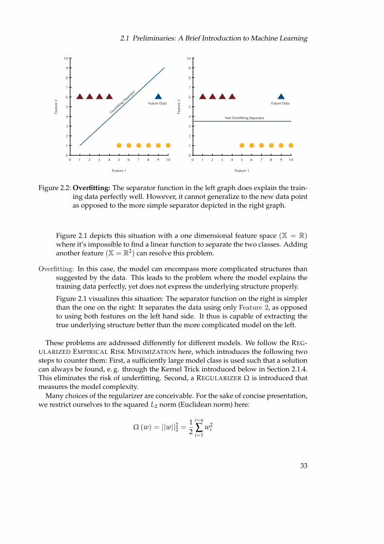
Not Overfitting Separator
Figure 2.2: Overfitting: The separator function in the left graph does explain the train-ing data perfectly well. However, it cannot generalize to the new data pointas opposed to the more simple separator depicted in the right graph.
Figure 2.1 depicts this situation with a one dimensional feature space (X = R)where it’s impossible to find a linear function to separate the two classes. Addinganother feature (X = R2) can resolve this problem.
Overfitting: In this case, the model can encompass more complicated structures thansuggested by the data. This leads to the problem where the model explains thetraining data perfectly, yet does not express the underlying structure properly.
Figure 2.1 visualizes this situation: The separator function on the right is simplerthan the one on the right: It separates the data using only Feature 2, as opposedto using both features on the left hand side. It thus is capable of extracting thetrue underlying structure better than the more complicated model on the left.
These problems are addressed differently for different models. We follow the REG-ULARIZED EMPIRICAL RISK MINIMIZATION here, which introduces the following twosteps to counter them: First, a sufficiently large model class is used such that a solutioncan always be found, e. g. through the Kernel Trick introduced below in Section 2.1.4.This eliminates the risk of underfitting. Second, a REGULARIZER Ω is introduced thatmeasures the model complexity.
Many choices of the regularizer are conceivable. For the sake of concise presentation,we restrict ourselves to the squared L2 norm (Euclidean norm) here:
Ω (w) = ||w||22 =12
i=n
∑i=1
w2i
33

2 The Machine Teaching Approach
Optimization
The training process of a machine learning model is an optimization problem: The empir-ical risk as well as the regularizer are minimized in a joint objective function:
O(w, X) = Remp (w, X) + λ Ω (w) (2.1)
= Remp (w, X) +λ
2
i=n
∑i=1
w2i (2.2)
Here, λ is a constant that defines the relative trade-off between the model complexityand the loss on the training data. An intuitive explanation of this observation can begiven as follows: A model is sought which agrees with the observed training data asmuch as possible (as measured through the empirical risk), but which on the other handis as simple as possible (as measured through the regularizer). This follows OCCAM’S
RAZOR which states that the simplest explanation that agrees with reality is the mostlikely one.
The result of the minimization is the model w which minimizes the objective functionO(w, X):
w = argminw (O (w, X)) (2.3)= argminw
(Remp (w, X) + λ Ω (w)
)(2.4)
To facilitate efficient optimization, the loss function is (re-)formulated as a convexfunction in the prediction f to facilitate efficient optimization. If the loss function isconvex in the prediction f , it is also convex in w for linear models. As the L2 normis convex in w, too, the whole training process then amounts to minimizing a convexfunction to find the model w which minimized the objective function (2.1).
In the binary classification case, the loss function is typically formulated as the HINGE
LOSS:
lHinge ( f , y) = max (0, 1− f y)This loss vanishes if the prediction f and the truth y agree. Additionally, the Hinge
Loss is a linear and therefore convex function in f . See Section 4.4.1 for a detaileddescription of the hinge loss. In Section 4.4 within the same Chapter, more examples ofloss functions are given, in particular for regression and ranking problems.
Given a convex loss function, the process of training the machine learning modelhas therefore been identified with that of optimizing a convex function. Numerousalgorithms are available for this task.
2.1.4 The Kernel Trick
The linear models above are of rather limiting expressiveness: If the data can only belinearly separated based upon the joint observation of two or more features, no linearmodel can be found that separates the data.
34

2.2 Introducing Machine Teaching
To heal this, one would have to define an additional feature that encodes the co-occurrence of the two other features to make the data linearly separable. The featureengineering therefore encodes non-linear features of the domain into dimensions of thefeature space to facilitate a linear model. This obviously is undesirable as it introducesa huge number of features of questionable relevance.
The concept of a kernel based algorithm as described e. g. in [SS02, Vap95, VGS97,Vap98] generalizes this idea to effectively turn most linear models to non-linear models.The process is commonly referred to as the KERNEL TRICK. To apply it to a linearmodel, one follows these steps:
1. One needs a formulation of the prediction rule as well as the optimization algo-rithm that does not operate on the samples x directly, but instead only uses innerproducts
⟨xi, x j
⟩between samples.
The inner products can be regarded as a measure of similarity between the sam-ples. Example: Let xi and x j be bag-of-words representations of texts as in theexample above. The inner product
⟨xi, x j
⟩then increases if xi and x j share more
words. It assumes the value of 0 if the texts do not share any word.
2. The invocation of the inner products⟨
xi, x j⟩
are then replaced with those of aKERNEL FUNCTION k(xi, x j). This function gives rise to a gram matrix Ki, j =k(xi, x j
). If that matrix is positive semi-definite
(xKx> ≥ 0 ∀x ∈ Rn), it can be
shown that the kernelized algorithm can be equated to a linear algorithm operat-ing in a space induced by that kernel.
The net effect of the application of this trick is: Many models that are linear in thesamples x can be transformed into models that are not linear in these samples. Thus,the trick has been applied to a wide variety of models to broaden their applicability.Major implementations can e. g. be found in the software package kernlab [KSH09,KSHZ04].
2.2 Introducing Machine Teaching
Building upon the general idea introduced in Chapter 1, Machine Teaching in the broad-est sense shall be defined as follows:
2.2.1 Definition
Definition 4 (Machine Teaching). MACHINE TEACHING conveys PRACTICED KNOWL-EDGE through machine learning models built from observational data of the application of thatknowledge.
It follows immediately from this definition that any machine learning model andmethod can be applied to in this sense. Consider the following hypothetical examplesof Machine Teaching applications:
35

2 The Machine Teaching Approach
Craft: A sequence prediction model can be built from observing experienced crafts-men. That model contains the knowledge about work sequences and can be ap-plied to support other craftsmen by providing hints on possible “next steps” intheir work.
Photography: Given the exposure data and e. g. light sensor input of a corpus of im-ages, a regression model can be trained to reflect the common exposure settingsused in certain light.
Writing in Novel Text Genres: Many genres of text found e. g. in communities on theworld wide web expose new styles of writing, spelling and even grammar. A ma-chine learned structure model of this grammar can be applied to support peoplenew to the community in writing for it.
Machine Programming: Many machines nowadays are controlled by computers andare therefore programmed for each product. Creating these programs requiresskill, experience and intuition. The performance of the programs is, however,rather explicit: The time it takes to produce the desired product, the amount ofwear and tear the production induced, etc. A machine learning model of theseprograms can be used to support new programmers and to foster the reuse ofknowledge from successful programs.
These examples show how broad the applicability of the approach is. In this thesis,we focus on a subset of the possible applications where the machine learning model isused to provide feedback to the learner in a way similar to the master in an apprentice-ship or master-student situation:
Definition 5 (Apprenticeship Machine Teaching). An APPRENTICESHIP MACHINE
TEACHING system supports learners during activities by providing ratings of and / or sugges-tions regarding these activities. It follows the concept of an apprenticeship where the apprenticeis offered ratings of and / or suggestions regarding her work from one or several experiencedpractitioners.
To provide these ratings and suggestions, a Machine Teaching system needs a machinemodel of the activity in question which captures the knowledge needed for this activity. Themodels are extracted from past observations of the same or similar activities by more experiencedpeople by means of machine learning.
Based upon these models and observational data about the activity of a learner, the MachineTeaching system generates ratings and / or suggestions and presents them to this learner.
Note that the term learning is overloaded in this thesis. It may either refer to thehuman learning or to the learning in the machine learning sense. Thus, we define:
36

2.2 Introducing Machine Teaching
Definition 6 (Learning). To distinguish between the two meanings of learning, we use thefollowing terms wherever the meaning is not clear from the context:
Learning denotes the learning of the humans, frequently called learners.
Machine Learning denotes the model building through a machine learning algorithm.
The same nomenclature is applied to the verb “to learn”, where we introduce the form “to ma-chine learn”.
2.2.2 High-Level Example of a Machine Teaching Scenario
Consider the following example taken from Chapter 6 to illustrate the idea of MachineTeaching:
Many of the practices in a team of programmers are never written down. Assumethat the practices include:
Whenever something is written to the database, we put an entry to the logfile starting with “Database Access:”.
A programmer new to the team will most probably hear about this practice onceshe fails to adhere to it: The fellow programmers will point out that mistake and theprogrammer will adhere to this practice in the future.
The latter process, pointing out the error, is where Machine Teaching is introduced:Given enough code, a model of that code can be machine learned. This model en-compasses the practice quoted above. Then, by observation of the code of the newprogrammer, the system can point out instances where the code does not match themachine learned model and thereby the practices formed by the team.
In this process, the Machine Teaching system assumes the role of the fellow program-mers in the current process. It is also apparent that the Machine Teaching system doesnot require the programming team to define or otherwise externalize their practices.Nor do the programmers have to provide the system with “model code” to learn from.Instead, the Machine Teaching system analyzed the code they already produced. Thissignificantly lowers the effort needed to deploy this Machine Teaching system whencompared to a more traditional technology enhanced learning system.
2.2.3 Machine Teaching Properties
Now that Machine Teaching has been defined, this and the following section providean analysis of the approach which follows from these definitions. In this section, theproperties of such a system are discussed, also contrasting them to those of a tradi-tional technology enhanced learning system. The section thereafter will explicate theassumptions regarding the learner and the scenario that underlie the Machine Teachingdefinition above.
It immediately follows from its definition that a Machine Teaching system is not de-pendent on externalized knowledge. The following paragraphs will introduce and discuss
37

2 The Machine Teaching Approach
additional important properties of any Machine Teaching system that falls within thescope of the definition above, while subsequent sections give insights on more specificinstances of Machine Teaching systems.
Machine Teaching can operate on non standardized knowledge: Machine Teaching ex-tracts the model from observational data. Thus, the knowledge that is needed toperform the observed activities needs not to be standardized. Depending on themachine learning model used and the amount of data available, even conflictingobservations can be co-existing in a Machine Teaching system.
Machine Teaching is focused on the practice, not the ideal: A Machine Teaching systemoperates on observations of activities and therefore has no access to the ideal wayof performing these activities. Such an ideal view would typically be found intraditional teaching materials such as textbooks and instructional videos.
Thus, a Machine Teaching system captures and subsequently teaches a differentquality of the activities when compared to traditional learning material: Howthey are done as opposed to how they should be done.
Machine Teaching is geared towards long-time use: Typical technology enhanced learn-ing tools such as an online course are focused on teaching the needed knowledgein a comparatively short period of time. Machine Teaching, on the other hand, ismore suitable in a long term setting: It provides feedback to the learner based onher activities. As these change over time, a Machine Teaching system can accom-pany the learner through different learning tasks, possibly even with an ambientlearning setting.
Depending on the use of a Machine Teaching system, it may constantly machinelearn by updating its model to the observed practices, too. Thus, not only thehuman learning is long-term, the machine learning is, too.
A Machine Teaching system makes mistakes: Even if the used machine learning mod-els capture the observed activities perfectly and make no mistakes (an unlikelycondition), these activities need not be executed perfectly at all. Thus, mistakesof a Machine Teaching system are to be expected just as mistakes of the humansobserved are to be expected, too.
However, these mistakes do not inhibit learning: The Machine Teaching systemmakes these mistakes based upon vast amounts of observations of past activities.Therefore, even if the Machine Teaching system makes an objectively false sug-gestion, it may still provide the learner with the information that her current ac-tivity is different from the mainstream as extracted from these observations. Thatinformation alone can therefore trigger important reflections within the learner.
Given these properties, it becomes apparent that Machine Teaching not only doesaway with the dependence on externalized, possibly structured knowledge but alsoexhibits teaching qualities which are new to the field of technology enhanced learning,such as being more suitable to teaching the practice as opposed to the ideal.
38

2.3 Major Components of a Machine Teaching System
It also became clear from this analysis that the performance of any future MachineTeaching system is crucially dependent on the quality of the available machine learningmodels and methods.
2.2.4 Machine Teaching Assumptions
In addition to these attributes of a Machine Teaching system, its definition also exhibitscertain assumptions regarding its applicability:
Data availability: Departing from traditional technology enhanced learning, MachineTeaching does not require externalized or even formalized knowledge. Instead,it requires observational data to build its machine model. Thus, it can only beapplied to domains where that data is available or can be gathered easily.
Availability of suitable machine learning techniques: As Machine Teaching relies on ma-chine learning models and methods at its core, only practiced knowledge thatcan be represented in those models can be conveyed through Machine Teachingsystem. However, any advance in the breadth and depth of available machinelearning techniques also adds new potential to the Machine Teaching approach.
Example: Machine translation is one active field of research in machine learn-ing. However, the techniques to machine learn to translate texts from pairs oftranslated texts have not matured enough to be considered for a Machine Teach-ing system. Once substantial progress is made in this field, a Machine Teachingsystem could be built that supports the education of human translators.
Learner Experience: An Apprenticeship Machine Teaching system provides ratings ofand / or suggestions regarding activities of the learner as observed by the system.It follows immediately that the learner needs to be capable at least of an attemptof the said activity. Otherwise, the Machine Teaching system will be unable toprovide meaningful feedback. Thus, the learners who use a Machine Teachingsystem cannot be complete novices of the field.
Situations where observational data is easily available and where learners have atleast minimal experience are plentiful, especially in the envisioned long-term usagescenarios.
2.3 Major Components of a Machine Teaching System
Departing from the rather abstract level of the definition and theoretical analysis ofMachine Teaching, a more systems-oriented perspective is taken in this section. Thefollowing introduces the major components of a concrete Machine Teaching system andtheir relations. This will not only facilitate a more detailed discussion in the remainderof this chapter but also provide the basis for an analysis of the research needed in orderto make Machine Teaching feasible.
39

2 The Machine Teaching Approach
Model Application
Machine Learning Method
Feedback Presentation
Expertsperforming an activity
Learnerperforming an activity
Trainingof the Machine Teaching System
Applicationof the Machine Teaching System
Legend:
: Sensors
Feedback
Machine Model
Figure 2.3: Major components of a Machine Teaching system. Note that the distinctionof users into Experts and Learners is introduced for clarity of presentationonly.
40

2.3 Major Components of a Machine Teaching System
Here, the components of a Machine Teaching system are introduced in two steps:First, they are described by themselves. Second, their dynamic interplay will be dis-cussed. Figure 2.3 shows the major components of a Machine Teaching system:
The Experts: These are the people that are observed by the system in order to machinelearn a model of the activity observed. The assumption regarding the experts isthat they perform the observed activity well enough to serve as an example forthe learner.
How to choose these experts in an application of Machine Teaching is specific tothat application. In the software engineering example above, the experts are thefellow programming team members of the learner as they have expert knowledgeon the practices established by that team.
The Learner: As introduced above, the learner is able to perform the activity to someextent, but requests or is presented assistance regarding her current activity. Thus,the learner may either be in an active role with respect to the Machine Teachingsystem or in the role of a consumer.
Note regarding these roles: Note that these two roles – experts and learners – arenot mutually exclusive. In fact, a learner may very well contribute to the system as anexpert, too. This may either be the case if the users of the system are experts in one partof the practiced knowledge and learners in another. Or, more interestingly, the MachineTeaching system could be used to accelerate consent-finding within a group of peers:All activities of all users contribute to the machine model of the practiced knowledge.And all users receive feedback from the system based upon that model which will yieldconsensual behavior of the users group.
The Sensors: Both the experts and the learner are monitored through these in order toprovide the Machine Teaching system with the observational data. The sensorsneed to be able to capture those attributes of the activity needed to perform thekind of assistance sought of the Machine Teaching system. While the sensorsexternalize data about the activity, this data hardly resembles knowledge.
Note that the sensors need not to be physical: In the Software Engineering exam-ple above, the sensors are formed by code analysis software.
The Machine Learning Method and Model: These two components are inter-dependentand thus are presented together. Given the sensor input, the machine learningmethod is used to learn the machine learning model. A chosen machine learningmodel can only be machine learned by a certain set of machine learning methods,hence the interdependence between the two.
The machine learning model (or machine model) is in principle chosen separatelyfor each application of Machine Teaching. However, we will introduce two majorclasses of Machine Teaching scenarios below, namely general and detailed feed-back, as well as appropriate machine model choices for both of them.
41

2 The Machine Teaching Approach
WorldDom.javaTest.javaDB.java
Editor
Others called log() in similar situations
Figure 2.4: Mockup of the user interface of a Machine Teaching System for program-mers.
Machine Teaching and machine learning are connected, as the abilities of the ma-chine learning method and model define the abilities of a Machine Teaching sys-tem. Any progress made regarding the accuracy, speed and expressive power ofthe underlying machine learning techniques directly reflects upon the same prop-erties of Machine Teaching approaches built upon these techniques.
The Feedback Generation Module: In this module, the observational data of the learner’sactivity is analyzed in order to provide ratings of and/or suggestions regardingthis activity. This module can be thought of as a two layered system:
The lower level consists of the application logic of the machine learning model tonew data. This level gets the sensor data as input and provides the higher levelwith its output, namely predicted rating of and / or suggestions regarding theobserved activity.
The higher level is responsible of presenting this information to the user. In thesoftware development example above, this could e. g. happen through a subtlehint as envisioned in Figure 2.4.
After describing the components of a Machine Teaching system, the following willintroduce the dynamic interplay of these components.
2.3.1 Dynamics of a Machine Teaching System
There are two phases to be considered in the analysis of the dynamics of a MachineTeaching system: The training phase and the application phase.
42

2.3 Major Components of a Machine Teaching System
Training Phase
In this phase, the system is presented observational data to machine learn a model ofthese observations. To do so, the sensory input first needs to be made accessible to theunderlying machine learning model and method. Subsequently, the actual training ofthe machine learning model through the machine learning method can occur, either inwhat is called offline or online learning:
Depending on the nature of the application of Machine Teaching, the observationaldata may either be available as one batch to train the system or arrive as a constantstream of data. The first case is called offline or batch learning in the machine learningliterature. The second case refers to online learning, which makes it possible for thesystem to constantly update its model upon the arrival of new data.
Obviously, the feedback generated by the Machine Teaching system cannot be en-sured to be constant and therefore predictable by the learner in the online learningcase. In fact, the system may very well contradict itself after machine learning fromnew data. These inconsistencies could inhibit the learning process. On the other hand,an online method facilitates a more current tracking of the practices observed by theMachine Teaching system which would lead to fewer inconsistencies between the feed-back provided by the Machine Teaching system to the learner and her observation ofthe practices of experts. Thus, the designer of a specific Machine Teaching system facesa trade-off between constant, predictable feedback and current feedback.
Application Phase
In this phase, the Machine Teaching system is presented observational data of thelearner’s activity and is sought to provide suggestions regarding and/or ratings of thisactivity. This can be thought of as a two-step process:
1. Potential feedback is derived from the machine learning model.
2. This feedback is presented to the learner.
The first step is again dependent upon the chosen machine learning model. But inaddition to this dependence, it also poses new requirements above the mere applicationof a machine learned model to new data: The learner needs instantaneous feedbackwhile in many other applications of machine learning, the results of the application ofthe model can be precomputed.
The second step does in principle not differ from the same step in a system wherethe feedback is not build upon machine learned models, but upon formalized knowl-edge embodied in the system. Example: In the software engineering example, it doesnot matter to the presentation layer whether the desired co-occurrence of logging anddatabase access is machine learned from data or hand coded as rules.
Performance of a Machine Teaching system: It became apparent not only from thesystems-oriented view above but also from the analysis provided earlier in this chapter
43

2 The Machine Teaching Approach
that the performance of a Machine Teaching system is largely determined by the per-formance of the machine learning method and model that supports it. All other factorssuch as user interface, data availability etc. being equal, a machine learning methodyielding higher accuracy, less error or better predictions in general will also yield amore satisfying Machine Teaching performance. Therefore, it is prudent to evaluatemachine learning models in Machine Teaching using the same or very similar tech-niques to those used in other machine learning applications.
2.3.2 Focus of this Thesis
So far, we have introduced Machine Teaching as a new approach to technology en-hanced learning. The remainder of this thesis presents a first step in investigating thisnew approach by studying its feasibility from a technological point of view.
To do so, we restrict ourselves to a critical set of components of a Machine Teachingsystem to study: We use the artifacts created by learners and experts as sensors andomit the feedback presentation layer from the analysis in the remainder of this thesis.The main research question in this thesis then is whether suitable machine learningmodels can be found or developed to support Machine Teaching systems in the future.The following paragraphs present the reasons for these choices.
Presentation of the feedback
The only component introduced above which is not discussed below is the presentationof the feedback to the learner. As mentioned earlier, this component does not differsignificantly from the very same component in systems where the suggestions givenby the system are hand-coded. Thus, it is safe to assume that such a module is easilydevised for a concrete Machine Teaching system.
The Sensors
For the purpose of this thesis, the sensors shall monitor the activities of users, learn-ers and experts alike, through their artifacts. While other sensor setups that monitorprocesses are conceivable, they also introduce severe challenges of their own that dis-tract from the research challenges of Machine Teaching addressed in this thesis. Thetechnology to reliably monitor human actions and correctly label those observationswith activities is still in the realm of research itself, dealing with challenges in sensortechnology, ambiguity in human action and not the least privacy concerns of the users.See e. g. [BMRC09] for an approach to classify group activities and e. g. [ZWS09] for anapproach to classify the activity of a single user based on sensors worn by that user.
Using artifacts to monitor the users does not suffer these drawbacks. For manydecades, whole areas of computer science such as computer vision, natural languageprocessing and speech analysis are devoted to the analysis of artifacts. Thus, a MachineTeaching system can tap into the results of these fields as a resource for the analysis ofthe artifacts.
44

2.4 General Feedback Machine Teaching
Many artifacts are created to serve a purpose. This also means that the extent towhich they serve this purpose, their quality, can be used as a factor to choose the arti-facts to train the Machine Teaching System on.
Additionally, artifacts can serve as an anchor in a multi-disciplinary collaboration:When people from different disciplines of expertise contribute to an artifact, the arti-fact and therefore the model machine learned from it contains representations of theknowledge from all these people and their respective disciplines. If that model is thenapplied to a situation where one or more of the disciplines are missing, the model canprovide important pointers to knowledge from other fields.
Machine Learning Method and Model
The main open question in studying the feasibility of Machine Teaching is whether ornot a machine learning model can capture the knowledge embodied in the artifacts.Following the task of a Machine Teaching system as defined above, we distinguishtwo levels of Machine Teaching: General Feedback Machine Teaching which aims atproviding grade-like ratings of the artifact and Detailed Feedback Machine Teachingwhich aims at providing suggestions regarding the artifacts.
The separation not only follows the two tasks of a Machine Teaching system, it is alsojustified from the state-of-the art of machine learning. As we will show below, generalfeedback can be devised using state-of-the-art machine learning techniques while theprovision of detailed feedback is more of a challenge to that field. Thus, general feed-back can serve as a testbed for Machine Teaching while detailed feedback needs furtherresearch regarding the machine learning techniques used.
The following two sections will describe these two levels of feedback in MachineTeaching in detail, including appropriate machine learning methods and models. Bothof these sections conclude with the identified research questions in there respective areato form the agenda of the remainder of this thesis.
2.4 General Feedback Machine Teaching
Closely following the definition of Machine Teaching, General Feedback Machine Teach-ing is defined as:
Definition 7 (General Feedback Machine Teaching). A GENERAL FEEDBACK MACHINE
TEACHING system provides the learner with “grade-like” numerical ratings of her artifact.To provide these ratings, a General Feedback Machine Teaching system extracts a model of theratings from similar artifacts rated by humans. Based upon this model and the artifact presentedto the system by the learner, the General Feedback Machine Teaching system generates ratingsand presents them to the learner.
It is important to note the difference between a system matching this definition andalready known systems: Computers have long been capable of rating artifacts, e. g.by matching them against a fixed set of rules. The spell checking facility found in
45

2 The Machine Teaching Approach
just about any modern desktop application is a good example of such a system. Ma-chine Teaching differs from these systems, as the rating computed is no longer basedon knowledge embodied in the system, but on models machine learned from ratedartifacts.
Appropriate Machine Learning Models
In this section, we identify machine learning technology needed to build a GeneralFeedback Machine Teaching system. From a machine learning perspective, the goal ofa General Feedback Machine Teaching system can be rephrased as: Given a set of ratedartifacts, find a model that is capable of predicting the rating for a yet unseen, unratedartifact.
This is virtually identical to the task of supervised machine learning systems as intro-duced above in Section 2.1. Depending on the type of the ratings, different approachessuch as classification or regression are appropriate.
Feature Engineering
Supervised machine learning approaches need a digital representation (denoted by x inthe definition above) of the artifacts. Typically, FEATURE VECTORS are used: One vectorrepresents one artifact. Each dimension of the vector refers to one feature (property,attribute) of the artifact and contains the value of that feature for this artifact.
Consider the following example from the field of Natural Language Processing (NLP):
Example 3. When dealing with text, the so called bag of words is a commonly used featurevector. For each document, a vector is constructed where each dimension represents the numberof times a certain word is present.
The text “This is an example within an example.” results in a feature vector where the valuein the dimensions for “This”, “is” and “within” is 1. The ones for “example” and “an” assumethe value of 2.
The process of determining the feature values for an artifact is called FEATURE EX-TRACTION, while FEATURE ENGINEERING refers to the finding, development and def-inition of the features. Much research in fields such as Natural Language Processingand Computer Vision resulted in a multitude of available features in their respectivedomains.
Key to the prediction performance of a supervised machine learning system andtherefore a General Feedback Machine Teaching system is to find appropriate featuresof the artifacts. In the worst case, where there is no relation between the artifact featuresextracted and its label, a supervised machine learning system cannot find a function tocompute the label from these features.
46

2.5 Detailed Feedback Machine Teaching
Research Questions
It also follows that the appropriateness of a feature is task-dependent: A feature thatis very successful in systems for one task does not necessarily perform equally well insystems built for other tasks.
As General Feedback Machine Teaching is a new task from the perspective of super-vised machine learning, the main research question can be phrased as:
Can features be found that allow a supervised machine learning system tobe part of a General Feedback Machine Teaching system?
This question is addressed via an example in Chapter 3. In that Chapter, features areproposed and evaluated for the task of estimating the rating of web forum posts. It willbe shown that features in fact can be found for this task.
To conclude, General Feedback Machine Teaching systems can be built and thus it isprudent to discuss the more ambitious goal of providing the learner with suggestionsregarding her artifact through a Detailed Feedback Machine Teaching system.
2.5 Detailed Feedback Machine Teaching
Again, we start the description of Detailed Feedback Machine Teaching with its defini-tion, closely following that of Machine Teaching in general:
Definition 8 (Machine Teaching). A DETAILED FEEDBACK MACHINE TEACHING systemsupports learners in the creation of artifacts by providing suggestions regarding these artifacts.
To provide these suggestions, a Detailed Feedback Machine Teaching system needs a ma-chine model of the artifact in question which captures structure of the kind of artifact in ques-tion. These models are extracted from similar artifacts created by more experienced people bymeans of machine learning.
Based upon these models and the artifact presented to the system by the learner, the MachineTeaching system generates suggestions and presents them to this learner.
The remainder of this section discusses the possible choices regarding a machinelearning model for this task. We will thereby identify open research questions thatare summarized at the end of this section.
Machine Learning Models
To provide suggestions regarding an artifact, a Detailed Feedback Machine Teachingsystem needs a grasp of the artifact’s structure. Similarly to the artifact features intro-duced above, this structure of the artifact is represented by structural elements of theartifact, which we define as:
47

2 The Machine Teaching Approach
Definition 9 (Structural Element). A STRUCTURAL ELEMENT of an artifact is a feature ofthe artifact that is mutable by the user, respectively learner of the system.
Structural elements are typed just as features are. Common types include binary, realvalued and one-out-of-n.
One artifact may be represented by a vector x of these structural elements, where eachdimension corresponds to one structural element. The value of the vector of one artifact inthat dimension is the value of the structural element. As an artifact is not required to have allstructural elements, the vector may be sparse.
The goal of Detailed Feedback Machine Teaching can then be stated as: Given thestructural elements of an artifact, suggest changes to the values of these or additionalstructural elements. Thus, the main difference to the goal of General Feedback MachineTeaching from a machine learning perspective is that instead of predicting a label y fora given sample x, the system is now asked to predict changes to the sample x.
In contrast to General Feedback Machine Teaching, this task does not map directly toone specific machine learning technique. In fact, one could design a statistical modelfor each artifact type and fit that model to the available data in principle. Graphicalmodels as introduced e. g. in [Bis06] (Chapter 8) provide the conceptual framework tobuild these models and henceforth machine learning algorithms for them.
The Connection to Recommender Systems
While the task of designing a model for each artifact type seems daunting, the followingobservation allows us to provide a machine learning model in a large set of DetailedFeedback Machine Teaching settings:
Observation: The process of suggesting (values of) structural elements ofartifacts is strikingly similar to that of suggesting products or services tousers in a Recommender System.
Recommender Systems are the enabling technology for many e-commerce vendorsand have found great research interest. The term “Recommender System” is often onlyimplicitly defined. For the sake of precision, the term shall be defined as follows for theremainder of this thesis:
Definition 10 (Recommender System). A RECOMMENDER SYSTEM suggests items tousers. The goal is to suggest those items to a user she is likely to like.
The recommendations are based upon available data about the user and the items, includinginteraction data between the users and items, e. g. in the form of user-supplied ratings.
In most cases, a recommendation is computed by first estimating the preference of the userfor the items and then presenting those with the highest estimates to the user. This core predic-tion logic of the system shall be referred to as RECOMMENDER ALGORITHM.
Following this definition, the observation above allows us to define Recommenderbased Machine teaching as:
48

2.5 Detailed Feedback Machine Teaching
Definition 11 (Recommender based Machine Teaching System). A RECOMMENDER
BASED MACHINE TEACHING SYSTEM suggests values of structural elements for artifacts.The goal is to suggest those values that fit the artifact well.
The suggestions are based upon available data about the structural elements and the arti-facts, including in particular similar artifacts as represented by their structural elements.
Requirements of a Recommender System
Despite this striking similarity, a Recommender based Machine Teaching system posesa specific set of requirements on the underlying recommender algorithm:
R1: Accurate solutions for partial artifacts: In its application, the Machine Teachingsystem needs to suggest values for structure elements based on partial artifactsas it is to support the learner during the creation of the artifact. Every time thelearner changes the artifact in ways that alter the structural elements, the systemneeds to compute new or adapted recommendations.
This is similar to the “new user” problem discussed in the Recommender Systemsliterature: A new user who has rated just a few items expects meaningful sugges-tions from the recommender system. The presence of new artifacts in this sense isthe norm in Machine Teaching scenarios, while it is the exception in a eCommercerecommender system.
R2: Interactive Performance: The Machine Teaching System shall be deployed suchthat it can provide accurate suggestions just-in-time: The Machine Teaching sys-tem must keep up with the speed the learner manipulates the artifact or, at least,the rate at which she demands suggestions from the system.
This is often less of a concern for commercial recommender systems, as the rate atwhich people buy items is considerably lower than the rate at which learners canmanipulate artifacts.
R3: Recommendation Coherence: The recommendations given by the Machine Teach-ing System may be subject to coherence restrictions such as in the following ex-ample:
Example 4. In the programming example in Section 2.2.2, the system should only recommendan operation on a String object if an object of that type is either present or its creation is alsosuggested.
Note that coherence requirements may be formalized in some cases, while in themore general case they are to be inferred from the data.
R4: Easy Adaptation to Multiple types of prediction: The structure elements of arti-facts may be of various types. Thus, the Machine Teaching System needs to beeasily adaptable to these changing types. Recommender algorithms, in contrast,are most often developed solely to predict the numerical rating a user would at-tach to a given item.
49

2 The Machine Teaching Approach
Available Recommender Algorithms
The Recommender Systems literature, e. g. in the survey paper [AT05] distinguishestwo different approaches: Memory based Recommender Systems and Model basedRecommender Systems.
Memory based Recommender Systems:1 To compute the predicted ratings, these sys-tems search for the users which are most similar to the one the prediction is madefor. The notion of similarity can be based on features as defined above, e. g. theirage or address, or it is based on past purchase data. Given those similar users, thepredictions is computed as the, potentially weighted, average of the labels givento the item in question by those users.
The same approach can be applied from an item perspective: A list of items isretrieved that are similar to the one in question. The weighted average over thelabels “given” to the user in question is the prediction of the system.
Model based Recommender Systems: Given past data, these systems build a model ofthe function that associates a user-item pair with a label. One approach to do sois to derive a function from the features of the users and items to the label. Asfor Memory based Recommender Systems, the model may also be defined on thepast purchase data of this and other users. Systems in that category are referredto as Collaborative Filtering Systems. Systems that make use of both user and itemfeatures and the collaborative information are referred to as Hybrid RecommenderSystems.
We will now investigate the suitability of these classes of Recommender Systems inthe light of the requirements described above.
Memory based recommender systems need to perform a search for similar artifactswhenever the learner requests assistance. In the desirable case where the MachineTeaching system can draw upon a large database of artifacts, this search considerablylimits the real time applicability of the system, violating requirement R2. We thereforeexclude memory based recommender systems from further analysis.
As stated in R1, a Machine Teaching System is frequently faced with new artifacts.These artifacts have only very few values for their structural elements and thereforeprovide little input to the recommender system to build its recommendation upon. Itis thus desirable to use a hybrid recommender system which is capable of using addi-tional features of the artifact and the structural element to enhance its prediction accu-racy.
Remaining Research Questions
However, to the best of our knowledge there is no model based hybrid recommendersystem that meets all of the requirements above. In Chapter 4, we present a novelrecommender algorithm that meets these requirements. The application of this newalgorithm to a Detailed Feedback Machine Teaching System for Software Engineers issubsequently presented in Chapter 6.
50

2.6 Conclusion
2.6 Conclusion
In this chapter, we introduced Machine Teaching as a new approach to Technology En-hanced Learning in which the knowledge formalization and externalization required intraditional Technology Enhanced Learning approaches is replaced with machine learn-ing: A machine learning model is built from observation of experts which is henceforthused to provide feedback to learners.
An analysis of the major components of a hypothetical Machine Teaching systemallowed us to determine a critical set of components needed to build such a system.This critical set of components and therefore the feasibility of a Machine Teaching isstudied in the remainder of this thesis from a technical perspective.
The remainder of this chapter presented two sub-categories of Machine Teaching sys-tems: Those providing a grade-like rating to the learner and those aiming at giving sug-gestions regarding the learner activity. The reason for this distinction lies not only in thetask but also, as we have shown, in the available machine learning techniques: Generalfeedback can be provided by supervised machine learning techniques, given suitablefeatures of the artifact. Detailed feedback, however, in principle requires specializedmachine learning models for each Machine Teaching task. But as we have shown, alarge subset of these tasks can be tackled using enhanced Recommender Systems tech-nology.
Next steps in this thesis: The remainder of this thesis is structured based upon thisobservation: In Chapter 3, we present a application of supervised machine learning tothe Machine Teaching task of rating web forum posts. Based upon the encouragingresults on this task, the Chapters 4 and 5 introduce a recommender systems model andalgorithm capable of meeting the Machine Teaching requirements outlined above. Thismodel and algorithm are then evaluated in the Machine Teaching task of providingsoftware engineers with detailed feedback in Chapter 6.
51

3 General Feedback Machine Teaching for WebForum Authors
Contents3.1 Introduction . . . . . . . . . . . . . . . . . . . . . . . . . . . . . . . . . . 54
3.1.1 Example domain . . . . . . . . . . . . . . . . . . . . . . . . . . . 543.2 State of the Art . . . . . . . . . . . . . . . . . . . . . . . . . . . . . . . . 55
3.2.1 Automatic Essay Scoring . . . . . . . . . . . . . . . . . . . . . . 563.2.2 Data Characteristics . . . . . . . . . . . . . . . . . . . . . . . . . 563.2.3 Feature Inspirations . . . . . . . . . . . . . . . . . . . . . . . . . 56
3.3 Feature Engineering . . . . . . . . . . . . . . . . . . . . . . . . . . . . . 573.3.1 Surface Features . . . . . . . . . . . . . . . . . . . . . . . . . . . 583.3.2 Lexical Features . . . . . . . . . . . . . . . . . . . . . . . . . . . . 583.3.3 Syntactic Features . . . . . . . . . . . . . . . . . . . . . . . . . . . 593.3.4 Forum Specific Features . . . . . . . . . . . . . . . . . . . . . . . 593.3.5 Similarity features . . . . . . . . . . . . . . . . . . . . . . . . . . 59
3.4 Evaluation Procedure . . . . . . . . . . . . . . . . . . . . . . . . . . . . 603.4.1 Data Set and Pre-processing . . . . . . . . . . . . . . . . . . . . . 603.4.2 Method . . . . . . . . . . . . . . . . . . . . . . . . . . . . . . . . . 61
3.5 Evaluation Results and Discussion . . . . . . . . . . . . . . . . . . . . 623.5.1 Results . . . . . . . . . . . . . . . . . . . . . . . . . . . . . . . . . 623.5.2 Performance Analysis . . . . . . . . . . . . . . . . . . . . . . . . 63
3.6 Conclusion . . . . . . . . . . . . . . . . . . . . . . . . . . . . . . . . . . 68
53

3 General Feedback Machine Teaching for Web Forum Authors
3.1 Introduction
In this chapter, the computational elements of a General Feedback Machine Teachingapproach are implemented and evaluated. The goal of a General Feedback MachineTeaching system is to provide the learner with “grade-like” ratings of her activity. Asintroduced earlier, we focus on observing the learner and the experts alike through theirartifacts.
From a machine learning point of view, General Feedback Machine Teaching is anapplication of the supervised learning techniques, as discussed in Section 2.4. In thesame section, we also identified feature engineering as the main challenge in buildinga General Feedback Machine Teaching system.
The remainder of this Chapter investigates the feasibility of a General Feedback Ma-chine Teaching system based on an example. The goal is not to present the best possiblesolution to the machine learning problems involved, but to show that building such asystem is indeed feasible. The chosen example domain, namely rating web forum posts,is introduced in Section 3.1.1. As there is no directly related or more so prior work, Sec-tion 3.2 presents prior research on useful features for this domain. Section 3.4 describesthe evaluation procedure and Section 3.5 presents the evaluation results on a real dataset.
3.1.1 Example domain
The example chosen for this evaluation is that of providing ratings of web forum posts.The goal of a General Feedback Machine Teaching system in this example can be phrasedas:
Given a set of human-rated forum posts, a machine model is learned that iscapable of predicting a rating for a yet unseen post.
We will now address the question why this is an interesting domain to apply MachineTeaching to. We will do so in three steps: First, we will introduce the example domainin greater detail to motivate it. Second, we will discuss the kind of knowledge involvedto motivate the inappropriateness of current technology enhanced learning systems.And lastly, we will present arguments why Machine Teaching should be applicable tothis task
Challenges in Teaching to Write for Web Forums
However, the posting habits between different web forums vary greatly. Thus, theknowledge needed to write posts that are regarded highly by the community of a givenforum cannot be (easily) transferred to another forum and thereby community. Thus,the task of teaching this knowledge through current technology enhanced learning ishard for the reasons discussed in Chapter 1.
54

3.2 State of the Art
Requirements for Machine Teaching to Write for Web Forums
In order to apply Machine Teaching, we need reliable data consisting of human-ratedweb forum posts, a machine learning technique to learn from this data and featureextraction procedures to make the data available to the machine learning algorithm.We will now briefly show that each of these requirements can be met in this domain:
Data Availability: Many websites such as Google Groups1, Yahoo! Groups2 and Nab-ble3 offer their users the possibility to rate forum posts in order to filter them.These ratings can be exploited by a Machine Teaching system.
Machine Learning Technique: As introduced earlier, we are facing a supervised ma-chine learning problem. As the field is well researched, the choice of a concretetechnique from this realm largely depends upon the type of rating in the data andsought from the Machine Teaching system.
Feature Engineering: Text has long been an application domain for machine learning,e.g. for SPAM filters, automatic text categorization or information retrieval sys-tems. Additionally, the natural language processing community has come upwith a countless amount of feature extraction procedures. Thus, we can tap intothis resource during feature engineering for the Machine Teaching system.
We can thus conclude the description of the example, Machine Teaching to write webforum posts, faithfully: It is a worthwhile example that poses serious challenges tocurrent technology enhanced learning technology but where all the requirements foran application of Machine Teaching are met.
Below, we will first introduce related research in Section 3.2 before devoting Sec-tion 3.3 to feature engineering. The Sections 3.4 and 3.5 present the evaluation proce-dure and results obtained with these.
3.2 State of the Art
To the best of our knowledge, there is no approach described in the literature that offersexactly the functionality sought in this chapter. There is, however, influential work inthe following areas that shall be discussed here:
• Approaches that have a similar goal to the one of Machine Teaching, but operateusing fixed rules, namely Automatic essay scoring systems.
• Works that investigate the characteristics of the collaborative rating data.
• Research that provides pointers to features to be extracted for the task at hand.
1http://groups.google.com2http://groups.yahoo.com3http://www.nabble.com
55

3 General Feedback Machine Teaching for Web Forum Authors
3.2.1 Automatic Essay Scoring
The automatic grading of texts has been investigated for quite some time in the researcharea of automatic essay scoring systems. Numerous systems and approaches have beendiscussed in the literature, e.g. in [CB04] and [AB06]. Valenti et al. present an overviewof the state-of-the-art in [VNC03].
These systems are based on the observation that there exists a fairly well defined no-tion of what a “good” essay is and how this manifests itself in detectable features ofthe essay. Additionally, essays tend to follow a very similar structure, at least thosethat are written to be graded by a teacher. The systems then detect these features of theessay as well as its structure using various heuristics and deduct a grade from these.So in essence, the grading function is not learned from data, but designed based on spec-ifications. This obviously is impossible in the web scenario, where each topic, websitesometimes each single web forum have distinct, implicit quality standards.
3.2.2 Data Characteristics
A question regarding the available data is whether the typically relatively few ratingsfrom a subset of the community can be assumed to be indicative of the community’sopinion at large. There is no data available on this subject for web forums, presumablydue to the high cost of obtaining it.
However, other websites, most prominently the IT news site Slashdot4, employ asophisticated meta-rating scheme that adds a pee-review of the ratings to the systemto ensure consistent ratings. Based on data from this peer review process from Slash-dot, Lampe and Resnick showed in their empirical study [LR04] that the rating data isindeed consistent: Disputes of the original rating are very rare events.
Whether or not this result can be transferred to web forums is hard to say, as theaudience of Slashdot, mostly IT students and professionals, is hardly representativefor Web users at large. This result does, however, show that consistent ratings areattainable. And as we will see later, we are able to predict the rating quite well whichfurther substantiates the conclusion that the ratings of posts found in web forums areconsistent.
3.2.3 Feature Inspirations
A track of research studies the behavior of students in web forums in conjunction withtheir academic success. In [KSF+06] it was found that there is a strong relation betweenstudent’s posting habits and their final grade even to the point that the grade can bepredicted from the posting habits. This supports our claim that writing well in forumsis an worthwhile skill to learn. The main features used in the grade prediction are thenumber of posts, the average post length and the average number of replies to postsof the student. Thus, it is worthwhile to investigate the same features for the MachineTeaching task at hand.
4http://www.slashdot.org
56

3.3 Feature Engineering
Kim et al. present a method to predict product review helpfulness in [KPCP06]. Inmany web shops, customers can review products both in text as well as formally usinga rating scale. Sites like Amazon also allow for the reviewing of these reviews to assurethe quality of the reviews submitted to the site. Readers of a review are asked “Wasthis review helpful to you?” with the answer choices “Yes” or “No”. These ratings arevery explicit and very standardized, as each reviewer is asked to rate the review basedon the same quality of the review, namely its helpfulness. Kim’s system than makesuse of the explicit content of the review in order to predict its helpfulness with greataccuracy. However, such a system is not easily transferable to the domain at hand fora number of reasons. The ratings a Machine Teaching System operates on cannot beassumed to be about the same quality dimension, with helpfulness being merely one ofthe choices as opposed to being the sole dimension of quality. Additionally, the systempresented in [KPCP06] gains much of its performance from the explicit content of areview, such as the numerical rating of the product discussed in the review. Clearly,such information cannot be assumed to be available in all Machine Teaching instances.The study [KPCP06] does, however, show that such structured data is very useful andshould be used whenever possible.
Summary: The related work suggests that the task of rating texts is possible, as ithas been done by human-designed systems before, albeit with an inherently limitedscope when compared to the aim of the approach presented in this chapter. The ratingdata underlying a machine learning approach can be assumed to be consistent with thecommunity, albeit the available data on that point is sparse. Lastly, we have briefly dis-cussed other machine learning based approaches operating on similar data to provideus with feature ideas for the task at hand.
The next step in investigating the feasibility of a General Feedback Machine Teach-ing system in the text domain is to present the features developed for the system inSection 3.3 before presenting the evaluation procedure and results in the Sections 3.4and 3.5
3.3 Feature Engineering
As mentioned earlier, feature engineering is the crucial step to the success of a super-vised machine learning application: While we can resort to an off-the-shelve supervisedmachine learning algorithm, feature engineering needs to be done for each applicationdomain separately.
In this section, the feature extraction procedures developed for the Machine Teachingsystem are described. As introduced in Section 2.4, the input data which consists ofunstructured text needs to be converted into vectors. This process is commonly referredto as feature extraction. Designing and implementing features for this task is mainly amanual process, which is guided by prior work and experience and intuition. Thus,feature engineering adds a systematic bias to the machine learning process at large, butone that is believed to aid in the learning task. For the system at hand, feature extractors
57

3 General Feedback Machine Teaching for Web Forum Authors
from five different classes have been built: Surface, Lexical, Syntactic, Forum specific andSimilarity features. The features and their extraction procedure are now described indetail.
3.3.1 Surface Features
The first class of features deals with properties of the text that are extractable on thecharacter level of the posts.
Length: It is hypothesized that the length of a post can have an influence on the qualityof it according to community standards. Thus, this feature captures the numberof tokens as reported by the tokenizer supplied by the Java SDK.
Question Frequency: The fraction of sentences ending with a question mark “?”. De-pending on the community, the presence or absence of questions and their fre-quency may be indicative of the perceived quality of the post.
Exclamation Frequency: The fraction of sentences ending with and exclamation mark “!”.Frequent use of exclamation marks is often considered rude in web forums.
Capitalized Word Frequency: The fraction of words spelled all CAPITALIZED. Wordsspelled like this are commonly associated with shouting in the conversation andare thus indicative of rude behavior.
3.3.2 Lexical Features
This class of features is concerned with the actual wording of the posts.
Spelling Error Frequency: It is commonly agreed that texts with a high fraction of mis-spelled words are considered bad. Thus, this feature detects the percentage ofwords that are not spelled correctly. In the experiments, the Jazzy spell checkingengine5 was used together with an English dictionary, as only English texts wereanalyzed.
Swear Word Frequency: This feature extractor stems from the same line of thought asthe extractors for the exclamation frequency and the capital word frequency: Rude-ness in the text might indicate poor quality according to the community stan-dards. Here, rudeness is detected rather directly by determining the percentageof words that are on a list of swear words. The list of swear words was compiledfrom public resources like WordNet and the Wikipedia. This swear word list con-tains more than eighty words like “asshole”, but also common transcriptions like“f*ckin” which occur frequently in web forum posts.
5http://jazzy.sourceforge.net
58

3.3 Feature Engineering
3.3.3 Syntactic Features
This class for feature extractors is concerned with the syntactic level of the texts ana-lyzed. To do so, the texts are annotated with part-of-speech tags as defined in the PENNTreebank tag set, see [MSM94].
To do so, the TreeTagger [Sch95] was used, parametrized by the parameter files forEnglish texts supplied with it. The fraction of each part-of-speech is then stored as onedimension in the resulting feature vector.
3.3.4 Forum Specific Features
The texts analyzed here stem from web forums, a genre of text that exhibits certainfeatures not present in other forms of text. The presence or absence of these specificfeatures may have an influence on the quality of the posts as perceived by the fellowusers of the same forum. The following features were extracted:
IsHTML: The users of a forum are usually offered some means to style their posts.In the case of the Nabble data used below, this was done using standard HTMLmarkup. This feature thus encodes whether or not the author of the post madeuse of this offering.
IsMail: Nabble also bridges mailing lists into web forums and vice verse. This featurecaptures the origin of a specific post, namely whether it is originally an email. Ifnot, the post has been entered through the web interface of Nabble.com.
Quote Fraction: When authoring a post, the user may choose to quote another post,e. g. to answer to a specific question raised in that other post. This is often con-sidered good style. However, some posts quote much without an obvious benefitto the post. This feature thus captures the fraction of characters within quotes ofa post to allow the machine learning model to capture this property.
Path and URL Counts: In forums where users help one another, a direct pointer to fur-ther information may be considered to be a good aspect of a post. In the experi-ments, two special kinds of pointers are considered: UNIX path names and URLs.Their number is counted and forms a feature in the feature vector.
3.3.5 Similarity features
Web forums are typically organized by topic. Posts which do not match the topic arecalled “off topic” and are usually considered to be bad posts. In order to capture therelatedness of a post to the topic it is posted in, the cosine between the word vector ofthe post and the word vector of the topic is used as an additional feature.
Note that this list of features is just an example of the feature engineering processrequired in the application of the Machine Teaching Process for general feedback. Inevery application, the set of features to extract needs to be re-evaluated.
59

3 General Feedback Machine Teaching for Web Forum Authors
Next steps: The remainder of this Chapter will focus on the evaluation of these fea-tures for the task of rating web forum posts, starting with describing the procedurefor doing so in Section 3.4. The following section will then present results from thatevaluation and present conclusions thereof.
3.4 Evaluation Procedure
In this section, we will describe the evaluation process used to evaluate the viability ofa General Feedback Machine Teaching system for rating web forum post. We describethe evaluation process in several steps:
• The data used for the evaluation is described and descriptive statistics of it arediscussed in Section 3.4.1. That section also goes into detail of the pre-processingand filtering of the data for the experiments reported in this chapter.
• The evaluation method is described in Section 3.4.2, including the cross-validationsetup and the choice of the supervised machine learning algorithm and imple-mentation thereof.
The results obtained using this experimental setup are presented in Section 3.5.
3.4.1 Data Set and Pre-processing
The data to evaluate the system was kindly provided by Nabble6. Nabble is a website that hosts forums for a wide range of communities and also mirrors mailing listconversations onto web forums. Below both kinds of content will be referred to as webforums.
The web forums hosted by Nabble are placed in a hierarchy, organized by their topic.Each forum is placed into exactly one category within this hierarchy. The discussionsin reach forum are further subdivided into conversation threads. All the posts in replyto the same post are part of one thread. As these posts may again attract replies, theforums forum a tree with posts and their respective answers as edges and leaves.
Posts at Nabble can be rated on a five star scale by the users, with five stars being thehighest rating. Analysis of the data showed that most of the rated posts are within the“Software” category7. To analyze the influence of the topic and thus the community onthe quality standards, the data was analyzed in three data sets:
ALL: All rated posts in the database. This is the broadest of all data sets.
SOFT: All rated posts of forums that are in the software category. These are posts thatconcern closely related.
6http://www.nabble.com7http://www.nabble.com/Software-f94.html
60

3.4 Evaluation Procedure
Stars Label ALL SOFT MISC? Poor 1928 45% 1251 63% 677 29%?? Below Avg. 120 3% 44 2% 76 3%
? ? ? Average 185 4% 69 4% 116 5%? ? ?? Above Avg 326 8% 183 9% 143 6%
? ? ? ? ? Excellent 1732 40% 421 21% 1311 56%
Table 3.1: Categories and their usage frequency at Nabble.
MISC: All posts that are in ALL, but not in SOFT. This data set is very diverse intopic, even more so than ALL, as half of ALL are posts from SOFT. Topics rangefrom discussions amongst Wikipedia community members to discussions of mo-tor bikes.
Table 3.1 shows the distribution of average ratings on the five star scale employedby Nabble. From this statistics, it becomes evident that users at Nabble prefer extremeratings. Therefore, the task of predicting the post quality can be considered as a binaryclassification task. Posts with less than three stars are rated as “bad”. Posts with morethan three stars are “good”.
Data Pre-processing
The goal of data preprocessing was to clean the data to a point where the label only con-tains variance stemming from the preceived quality of the forum posts. To do so, ostswith an average rating of exactly 3 were removed, as they cannot be attributed to anyof the binary classes. Manual analysis of posts with contradicting votes on the binaryscale revealed that they were mostly spam, which was voted high for commercial inter-est by account associated with the poster and voted down for being spam. Thus, theseposts were removed, too. We also filtered out the posts that did not contain any text,but only attachments like pictures and program files as the quality of these posts cannotbe attributed to the textual content. Finally, we removed non-English posts using a sim-ple heuristics: Posts that contained a certain percentage of words above a pre-definedthreshold, which are non-English according to an English dictionary, were consideredto be non-English.
The upper part of Table 3.2 shows how many posts were removed from the threedata sets. Note that we did the filtering independently for each filter. Thus, posts thatmatched several filtering criteria contribute more than once to the statistics. The lowerpart of that table shows the distribution of good and bad posts after filtering.
3.4.2 Method
Using the feature extractors described above, we compiled a feature vector for eachpost. Feature values that were not normalized by definition were scaled to the range
61

3 General Feedback Machine Teaching for Web Forum Authors
ALL SOFT MISCUnfiltered Posts 4291 1968 2323
All ratings three stars 135 3% 61 3% 74 3%Contradictory ratings 70 2% 14 1% 56 2%
No text 56 1% 30 2% 26 1%Non-English 668 15% 361 18% 307 13%
Remaining 3418 80% 1532 78% 1886 81%
Good Posts 1829 54% 947 62% 1244 66%Bad Posts 1589 46% 585 38% 642 34%
Table 3.2: Number of posts filtered out in the different data sets.
[0.0, . . . , 1.0]. To classify the posts, we use support vector machines. In particular, weused a SVM with a Gaussian kernel as implemented in the LibSVM module in the YALEtoolkit [MWK+06] in all experiments.
We perform stratified ten-fold cross validation for performance evaluation. The datais split into ten sub sets where each exhibits the same class distribution as the full dataset. The system is then trained on nine of these sub sets and evaluated on the last. Wereport the mean results of all ten evaluations.
Several randomly chosen experiments were repeated using the leave one out eval-uation scheme. There, the system is trained on all but one post and evaluated on theremaining one. The average over all runs over all data points is returned as the per-formance metric. These experiments yielded comparable results to the ones obtainedusing cross validation. Thus, we only report the latter.
3.5 Evaluation Results and Discussion
In this section, we present and discuss the evaluation results obtained through the pro-cedure introduced in the previous section. We first present the empirical results inSection 3.5.1. In Section 3.5.2, we discuss the errors the system makes to allow us todraw the conclusions presented in Section 3.6.
3.5.1 Results
Table 3.3 shows the average cross validation accuracy for all combinations of featureand data sets when compared to a baseline system. Note that we did not perform pa-rameter tuning for the different feature sets but kept the parameters fixed8 and thereforeminor performance gains may still be possible.
8The parameters where fixed to λ = 0.1 and σ = 0.1.
62

3.5 Evaluation Results and Discussion
Baseline: A baseline system is a simple system that serves as a plausibility check ofthe results obtained. In our case, we employ a majority-class classifier as the baseline:Such a classifier always predicts the class which had the majority of instances in thetraining data. Example: If 70 % of the posts in the training data are labeled as goodposts, the majority class classifier labels all unseen posts as good. Clearly, any moresophisticated machine learning system should outperform this baseline.
As shown in Table 3.3 , all results but one (SIM/ALL) are equal to or better than thebaseline. The usage of all features results in the best or close to best performance for alldata sets. The results on the MISC data set are only slightly better than the baseline. Thegains on the SOFT and ALL data sets over the baseline are significant. Naively, one maythink that the performance on the ALL data set is the average between the performanceon MISC and SOFT, as both form approximately one half of the data in ALL. The resultsare different, and the performance on ALL is comparable to the performance on SOFT.Thus, the system is able to learn how to classify posts in MISC from posts in SOFT. Itis thus plausible to assume that the rating structure in some posts of the MISC data setis very close to the SOFT data set, while the overall rating structure is too diverse to becaptured correctly by the system.
The difference in rating structure also shows in the analysis of the best performingfeature categories, which are different for each data set. For MISC, the surface featuresperform best. For SOFT, the forum specific features work best, when only one featurecategory is used.
It is useful to have a look at the performance of all other feature categories, whenthe single best one is not present to assess the influence of the best feature category onthe overall performance. For MISC, this leads to a performance on the baseline level.For SOFT, the drop in performance is much smaller, yet still measurable. For ALL, theeffects are the smallest, being almost zero for the removal of the lexical features.
To evaluate the features in more detail, additional experiments were performed onthe SOFT data set with only the features from the best performing category, namelythe Forum specific features. Table 3.4 shows that IsMail and Quote Fraction are thedominant features. This is noteworthy, as those features are not based on the domainof discussion.
3.5.2 Performance Analysis
In addition to the numerical evaluation presented above, we will now present a moredetailed analysis of the performance of the system.
The first step to do so is to investigate more closely what kind of errors contributedto the average accuracy presented above through confusion tables. In a second step,we present a qualitative evaluation of frequent mistakes of the system. Besides point-ing out open issues in the currently implemented system, the latter allows us to drawconclusions regarding the inherent limits of the approach.
63

3 General Feedback Machine Teaching for Web Forum Authors
SUF LEX SYN FOR SIM ALL SOFT MISC√ √ √ √ √77.53% (1.45) 89.10% (1.44) 71.95% (1.09)√
– – – – 64.72% (1.21) 61.82% (1.00) 71.31% (1.08)–
√– – – 74.08% (1.38) 71.82% (1.16) 65.96% (1.00)
– –√
– – 69.18% (1.29) 82.64% (1.34) 66.70% (1.01)– – –
√– 74.08% (1.38) 85.05% (1.36) 65.96% (1.00)
– – – –√
46.49% (0.87) 62.01% (1.00) 65.96% (1.00)–
√ √ √ √75.92% (1.42) 89.10% (1.44) 66.60% (1.01)√
–√ √ √
77.39% (1.45) 89.36% (1.46) 72.00% (1.09)√ √–
√ √76.27% (1.43) 85.03% (1.38) 70.03% (1.06)√ √ √
–√
72.82% (1.36) 82.90% (1.34) 71.74% (1.08)√ √ √ √– 76.83% (1.44) 88.97% (1.44) 72.43% (1.10)
Baseline 53.51% (1.00) 61.82% (1.00) 65.96% (1.00)
Table 3.3: Accuracy with different feature sets. SUF: Surface, LEX: Lexical, SYN: Syntax,FOR: Forum specific, SIM: similarity. The baseline results from a majority classclassifier.
Confusion Tables
Confusion tables present the performance of a system in more detail by showing thenumber of all four performance relevant cases of a binary classifier:
True Positives: These are posts that are labeled as good by the users and are predictedto be good posts by the system.
True Negatives: Posts which are labeled and correctly predicted to be bad.
False Positives: The system incorrectly predicted a good label for these posts, whilethe users labeled it as bad.
False Negatives: In the last case, the system predicted a bad label while the users actu-ally labeled the post as good.
Depending on the system evaluated, a balanced or unbalanced rate of false positivesand false negatives may be desired. Example: In the case of an email spam filter, onetypically wants to minimize the number of emails that are falsely labeled as spam bythe system, even if that means to compromise the rate of spam caught by the filter.
In Machine Teaching, a balanced performance is more desirable to allow the learnerto draw her own conclusions from the rating presented to her.
Tables 3.5, 3.6 and 3.7 contain the confusion tables for the system using all featureson the three different data sets. The system produces approximately an equal amountof false positives and false negatives on the ALL and SOFT data sets. However, it hasa tendency towards false positives on the MISC data set. This indicates that systems
64

3.5 Evaluation Results and Discussion
ISM ISH QFR URL PAC Avg. accuracy√ √ √ √ √85.05%√
– – – – 73.30%–
√– – – 61.82%
– –√
– – 73.76%– – –
√– 61.29%
– – – –√
61.82%–
√ √ √ √74.41%√
–√ √ √
85.05%√ √–
√ √73.30%√ √ √
–√
85.05%√ √ √ √– 85.05%√
–√
– – 84.99%√ √ √– – 85.05%
Table 3.4: Accuracy with different forum specific features. ISM: IsMail, ISH: IsHTML,QFR: QuoteFraction, URL: URLCount, PAC: PathCount.
should be trained separately for different topics of discussion and therefore user com-munities.
Qualitative Analysis of important System Errors
Below, we will give descriptions of common errors of our system as well as some ex-amples from the data. We will also provide conclusions on how to improve the currentsystem to overcome the errors where possible and indicate errors which exemplify theinherent limits of the approach.
Ratings based on domain knowledge: The following post from the SOFT data setshows no apparent reason to be rated badly. The human rating of this post seems to bedependent on deep domain knowledge, which cannot be represented in the MachineTeaching System easily. Thus, these posts are part of the inherit limits of the approach.
65

3 General Feedback Machine Teaching for Web Forum Authors
true good true bad sumpred. good 1517 456 1973
pred. bad 312 1133 1445sum 1829 1589 3418
Table 3.5: Confusion matrix for the system using all features on the ALL data sets.
true good true bad sumpred. good 490 72 562
pred. bad 95 875 970sum 585 947 1532
Table 3.6: Confusion matrix for the system using all features on the SOFT data sets.
true good true bad sumpred. good 1231 516 1747
pred. bad 13 126 139sum 1244 642 1886
Table 3.7: Confusion matrix for the system using all features on the MISC data sets.
Example 1.> Thank You for the fast response, but I’m not> sure if I understand you right. INTERRUPTs can> be interrupted (by other interrupts or signals) and> SIGNALS not.
Yup. And I responded faster than my brain could shift gearsand got my INTERRUPT and SIGNAL crossed.
> All my questions still remain!
Believe J"org addressed everything in full. That thecompiler simply can’t know that other routines have leftzero reg alone and the compiler expects to find zero there.
As for SREG, no telling what another routine was doing with thestatus bits so it too has to be saved and restored before anyof its contents possibly get modified. CISC CPUs do this foryou when stacking the IRQ, and on RTI.
66

3.5 Evaluation Results and Discussion
Automatically generated mails: Sometimes, automatically generated mails like errormessages end up on the mailing lists mirrored by Nabble. These mails can be writtenvery nicely and are thus misclassified by the system as good posts, while they are badposts from the point of view of the users. These errors are conceptually easy to avoidby pre-processing. In fact, these posts should never be used for a Machine Teachingsystem, as there is little to learn from them.
Non-textual content: Especially the SOFT data set contains posts that mainly consistof non-textual parts like source code, digital signatures and log messages from pro-grams. This content confuses our system to miss-classify these posts as bad posts eventhough the sheer presence of these parts may be very useful to the reader.
To overcome this problem, the non-textual parts need to be marked. They can thenbe ignored in the quality assessment of the textual content. Additionally, the presenceand the amount of non-textual content can be used as an additional feature. A DetailedFeedback Machine Teaching system could then even suggest to the learner to attachsupporting material to make their post more valuable to the readers.
Very short posts: Posts which contain only a few words show up as false positives andfalse negatives equally, as for example a simple “yes” from the grand master of a certainfield might be regarded as a very good post, while a short insult in another forum mightbe regarded as a very bad post. For Machine Teaching, it thus seems advisable not torate very short posts at all, as the system is very likely to rate the post wrong and thusto confuse the learner.
Opinion based ratings: Some ratings do not rate the quality of a post, but the expressedopinion. In these cases, the rating is an alternative to posting a reply to the messagesaying “I do not agree with you”.
Take for example the following post which is part of a discussion amongst Wikipediacommunity members from the MISC data which has been misclassified as a bad post:
Example 2.> But you would impose US law even in a country where> smoking weed is legalGiven that most of our users and most significant presscoverage is American, yes. That is why I drew the line there.Yes, I know it isn’t perfect. But it’s better than anythingelse I’ve seen.
Such posts form a hard challenge for automatic systems. However, they may alsoform the upper bound for this task: Humans are unlikely to predict these ratings cor-rectly without additional knowledge about the rater, either.
67

3 General Feedback Machine Teaching for Web Forum Authors
3.6 Conclusion
We studied the machine learning aspects of a General Feedback Machine Teaching sys-tem for web forum post writing in this chapter. The goal of this study was to answerthe question whether suitable features can be found that allow a supervised machinelearning method to rate the forum posts well.
The quantitative evaluation presented in this chapter suggests that such featureshave indeed been found as the system achieves an average accuracy of up to 90 %.The qualitative study also substantiates the claim that proper feature engineering is thekey factor for the predictive performance of the system.
The qualitative analysis of the results also suggest important considerations and lim-its for Machine Teaching:
• Not all ratings given by humans can be predicted by a machine. The examplesfound in the qualitative study are ratings that express opinions and those whichrequire deep domain knowledge to be given.
• Data pre-processing for Machine Teaching should be done in addition to the pre-processing done to allow the machine learning system to perform well. The studyin this chapter follows machine learning best practices when it comes to pre-processing such as filtering ambiguously rated posts. The quantitative analysis ofthe system’s performance however revealed additional need for pre-processing:The data contained artifacts such as automatically generated content that shouldnot be part of the training data for a machine teaching system.
• The accuracy of the system on short posts is to low, even if above random, tojustify presenting the predicted ratings to the learner.
Besides the hard limits in machine predictability of human behavior inherent to theapproach, all of these considerations can be addressed through engineering.
Thus, and given the good overall performance of the system, it is safe to concludethat the state-of-the-art machine learning techniques as well as the best practices in thefield can be applied to build General Feedback Machine Teaching systems.
Next steps in this thesis: Given this conclusion, the remainder of this thesis departsfrom General Feedback Machine Teaching and focuses on the task of Detailed FeedbackMachine Teaching. As this task is more ambitious from a machine learning perspective,Chapter 4 presents an algorithm that forms the foundation for addressing this task.Chapter 5 leaves the field of Machine Teaching in order to evaluate that algorithm onwell established Recommender Systems tasks. This allows us to compare the algorithmperformance to that of the state-of-the-art in that field. In Chapter 6, a similar study tothe one in the present chapter is described, albeit for the Detailed Feedback MachineTeaching case.
68

4 Generalized Matrix Factorization
Contents4.1 Introduction . . . . . . . . . . . . . . . . . . . . . . . . . . . . . . . . . . 704.2 State of the Art . . . . . . . . . . . . . . . . . . . . . . . . . . . . . . . . 714.3 Regularized Matrix Factorization . . . . . . . . . . . . . . . . . . . . . 734.4 Loss Functions . . . . . . . . . . . . . . . . . . . . . . . . . . . . . . . . 76
4.4.1 Element Based Loss Functions . . . . . . . . . . . . . . . . . . . 764.4.2 Row Based Loss Functions . . . . . . . . . . . . . . . . . . . . . 794.4.3 A faster Ordinal Regression Loss Function . . . . . . . . . . . . 804.4.4 An NDCG Loss Function for Matrix Factorization . . . . . . . . 854.4.5 Conclusion . . . . . . . . . . . . . . . . . . . . . . . . . . . . . . 92
4.5 Optimization . . . . . . . . . . . . . . . . . . . . . . . . . . . . . . . . . 924.5.1 Optimization over the Row Matrix R . . . . . . . . . . . . . . . 954.5.2 Optimization over the Row Matrix C . . . . . . . . . . . . . . . 954.5.3 New Row Optimization . . . . . . . . . . . . . . . . . . . . . . . 96
4.6 Extensions to the Regularized Matrix Factorization Model . . . . . . 964.6.1 Row and Column Biases . . . . . . . . . . . . . . . . . . . . . . . 964.6.2 Adaptive Regularization . . . . . . . . . . . . . . . . . . . . . . . 974.6.3 Structure Exploitation with a Graph Kernel . . . . . . . . . . . . 984.6.4 Row and Column Features . . . . . . . . . . . . . . . . . . . . . 98
4.7 Conclusion . . . . . . . . . . . . . . . . . . . . . . . . . . . . . . . . . . 99
69

4 Generalized Matrix Factorization
4.1 Introduction
This chapter introduces a novel model and algorithm for the problem of matrix factor-ization. Before doing so, it is shown how both the Recommender System problem andmany Machine Teaching settings can be rephrased into matrix factorization instances.
We will first show that the available data in both Recommender Systems and Ma-chine Teaching can be thought of as a sparse matrix Y for which a dense approximationis sought. The entries at the formerly sparse points of this approximation constitutethe prediction. This view on the data is visualized in Figure 4.1 and described in thefollowing paragraphs:
Machine Teaching with Matrix Factorization: In a Machine Teaching setting, each rowin Y corresponds to one artifact. The columns of Y contain the values of the struc-ture elements of this artifacts. This matrix is typically sparse, as not all artifactsexhibit all structure elements. To give detailed feedback for the learner, the Ma-chine Teaching System needs to deduct a model from the data which can computea dense matrix F which contains predictions for the sparse points in Y. In contrastto the recommender system setting, the Machine Teaching system may not onlymake use of the predictions for the sparse entries of Y but also of the discrepancybetween the known entries in Y and those in the model F, e. g. to correct thelearner.
Recommender Systems with Matrix Factorization: In Recommender Systems, Y hasas many rows as there are users and as many columns as there are item. Theentries Yi, j of this matrix are the label given to item j by user i. The type of theseentries depends on the kind of label available in the specific data set. Note thatthis matrix is very sparse. In a typical movie recommender scenario, there are inthe order of twenty thousand movies and thus columns in Y. Not many usershave watched and rated all these movies. The goal for the recommender systembased on this sparse matrix Y is to find a dense matrix F of equal dimensions thatcontains predictions for the user-item pairs not present in Y.
The algorithm described in this chapter is applicable to both scenarios: MachineTeaching and Recommender Systems. This is due to the fact that it operates on therather abstract level of matrices as opposed to their real world correspondences of arti-facts, structural elements, users and items.
Honoring this aspect and to facilitate a broad view on the algorithm, the remainderof this chapter is written in an application-agnostic manner. We will give examplesfrom both the Machine Teaching and the Recommender Systems perspective whereappropriate.
In this application-agnostic notation, the goal of the algorithm can be phrased as:Given a potentially sparse input matrix Y ∈ Tr×c find a dense matrix F ∈ Tr×c thatexplains Y well and predicts entries for the sparse elements in Y.
70

4.2 State of the Art
Struc
tural
Elemen
t A
1 – 1 3 …
– 0 7 – …… … … … ……
…
Y
Struc
tural
Elemen
t B
Struc
tural
Elemen
t C
Struc
tural
Elemen
t D
Artifact 1Artifact 2Artifact 3Artifact 4Artifact 5Artifact 6
Item A
2 1 5 – …
0 – 3 1 …… … … … ……
…
Y
Item B
Item C
Item D
User 1User 2User 3User 4User 5User 6
Machine Teaching Recommender Systems
Figure 4.1: Modeling the available data in a Detailed Feedback Machine Teaching Sys-tem (left) and in a Recommender System (right) as a sparse matrix Y. Thesymbol “–” indicates a sparse point (missing value)
4.2 State of the Art
The development of factor models and in particular matrix factorization methods are anactive field of research. Factor models have shown remarkable performance in manyinstances, especially in the context of the Netflix prize challenge where all of the topcontenders use factor model based approaches.
In matrix factorization methods, the data is assumed to be contained in a sparse ma-trix Y ∈ Tr×c (Yi, j in Recommender Systems typically indicates the rating of item j byuser i). The basic idea of matrix factorization is to fit this matrix Y with a low rank ap-proximation F. Here, F is computed as F = RC> where R ∈ Rr×d and C ∈ Rc×d. Morespecifically, the goal is to find an approximation that minimizes a loss measure such asthe sum of the squared distances between the known entries in Y and their predictionsin F.
Below, we introduce major means of finding the approximation F, starting with Sin-gular Value Decomposition before discussing the Regularized Matrix Factorization tech-nique that the algorithm presented here is built upon. The last part of this section willbe devoted to the related work on seemingly binary input matrices Y.
Singular Value Decomposition One way of doing this is to compute a Singular ValueDecomposition of Y and to use only a small number of the vectors obtained by thisprocedure. In the information retrieval literature, this numerical operation is commonlyreferred to as Latent Semantic Indexing as introduced in [Hul94].
Note, however, that this method does not do justice to the way Y was formed as Y issparse. This fact is ignored by the SVD and depending on the specific implementation,
71

4 Generalized Matrix Factorization
the sparse elements in Y are assumed to be 0 or are replaced with averages in order tocompute the SVD. Both approaches potentially misinterpret the data. If e. g. a user didnot rate an item this may correspond to a variety of reasons that cannot be capturedby these assumptions. Many rating schemes assume lower ratings to be worse, andfilling in the sparse elements with ratings of 0 assumes that the user did not like thesemovies. The filling with (per user) averages fares slightly better, but that assumption isquestionable in many instances, too.
The filling poses even more of a problem in Machine Teaching where each value of astructure element may have an impact on the artifact quality. Both 0 and the the averagevalue of the remaining elements are likely completely unrelated to a reasonable valueto be filled in. Even worse, this approach ignores the fact that the sparse elements in Yare the requested output of the algorithm and should thus not be used as input.
Regularized Matrix Factorization In [SJ03], an alternative approach is suggested whichaims to find a factorization of Y in two matrices R ∈ Rr×d and C ∈ Rc×d such thatF = RC> with the goal to approximate the observed entries in Y rather than approxi-mating all entries at the same time. This approach has been shown to work well on e. g.rating data from users on movies such as in the Netflix price competition.
Minimizing the rank of F is intractable in practice for all but the smallest problems.Instead. the question of capacity control of the resulting predictor has been addressedin [RS05] and [SRJ05] by means of matrix norms on F. It has been shown in [SS05]that the Frobenius norm on R and C is a proper norm on F and can thus be used forcapacity control. In addition, they proposed a multi-class version of the hinge lossfunction that together with the Frobenius norm induces a large margin solution. Theterm Maximum Margin Matrix Factorization (MMMF) has thus been coined for this ap-proach in [SRJ05]. Similar ideas based on matrix factorization have also been proposedin [TPNT07] and in [SM08, BKV07] which mainly focus on improving performance onthe Netflix data set. In [SG08] an integration of these different approaches into onemodel is presented. Note that all these methods are colloquially referred to as “SVD”or “SVD-style”, even though they do not use a SVD in the strict sense.
None of these approaches address the problem of a prediction that needs to be con-sistent per-row as required in the Machine Teaching setting.
Binary data In many instances, the data is seemingly binary, for example when build-ing a Machine Teaching System for software engineering:
Example 5. We will later model code as a matrix of caller-callee relations. An entry of Yi, j = 1in this matrix indicates a call of caller i to callee j. However, the opposite entry cannot beattributed to a single cause. The absence of a call can e. g. be attributed to a conscious decisionof the programmer or a bug. Any of these cases will be encoded as a sparse and thus missingentry in Y, as the true reason typically is unknown.
Note that the same effect also occurs in commercial Recommender Systems that op-erate on shopping basket data: There, it is only known for sure whether a customer
72

4.3 Regularized Matrix Factorization
bought an item. The information that a customer did not buy an item can be attributedto a variety of reasons, including being unaware of the item. In that case, a recommen-dation should be considered for the item. Thus, it is not advisable to equate the absenceof a buy with a dismissal of the item by the customer.
We refer to seemingly binary data like this as dyadic interaction data. It can be rep-resented as a sparse matrix where Yi, j = 1 indicates that an interaction between rowi and column j was recorded. In Machine Teaching such an entry indicates that theartifact i has the structural element j. In a Recommender System it indicates that user iinteracted with item j, e. g. by renting the movie j.
Traditionally, rule and memory based systems have been applied in these situations(see e. g. [AT05]). As discussed in Section 2.5, one of the shortcomings of memory basedsystems is that the prediction time scales super linearly with the number of trainingsamples. This poses a serious restriction, as these systems cannot be used interactivelyany more when the number of available training data rises which poses a serious limita-tion on the applicability of these systems to Machine Teaching scenarios where instantfeedback is required.
Several approaches have been introduced under the term “binary matrix factoriza-tion”, see e. g. [ZDLZ07]. In these systems, R and C are assumed to be binary, too. How-ever, this drastically limits the applicability, as finding these matrices then amounts tosolving combinatorial optimization problems. Other approaches based on binary latentfactors [MGNR06] and Gaussian processes [YC07] extract binary factors as well whichinduce constrains that would not be particularly useful in the recommender settingwe are considering and provide little control over the treatment of unlabeled values ornegative examples in the data.
Conclusion: The state of the art provides a solid theoretical and empirical base formatrix factorization approaches. However, most systems do not make use of features,even though their addition is rather straight forward as we will discuss below. Usingfeatures is crucial for a Machine Teaching System and helps considerably in overcomingthe new user and new item problems in Recommender Systems.
None of the approaches can deal with per-row predictions as they arise in MachineTeaching and ranking prediction in Recommender Systems. Binary data provides aformidable and essentially unsolved challenge.
4.3 Regularized Matrix Factorization
In this section, the notion of Regularized Matrix Factorization is presented in greaterdetail to allow us to use it as a framework in which to present our algorithm.
As noted earlier, the algorithm presented here is based on the idea of Factor Models:Each known entry Yi, j is hypothesized to be explainable by a linear combination of drow factors Ri ∈ Rd and d columns factors C j ∈ Rd:
Fi, j := 〈Ri, CJ〉 (4.1)
73

4 Generalized Matrix Factorization
Symbol Type DescriptionY Tr×c The sparse input matrixF Tr×c The dense prediction matrixR Rr×d The dense matrix of row factorsC Rc×d The dense matrix of column factorsr N The number of rows in Yc N The number of columns in Yn N The number of entries in YT – The entry type in Y and F
L(F, Y) Tr×c ×Tr×c → R The loss functionΩ(F) Tr×c → R The regularizer
λr, R The regularization parameter for Rλc R The regularization parameter for CS 0, 1r×c Si, j = 1 for values present in Y and 0 otherwise.
g(y) R The weight associated with the label y in theweighted loss functions.
y, f Tc Dense versions of a row in Y and F where thesparse elements of Y have been omitted.
Table 4.1: Symbols used
Matrix Factorization models built upon this idea by noting that in effect, F is con-structed as the multiplication of two matrices R ∈ Rr×d and C ∈ Rc×d:
F := RC> (4.2)
While this model allows to compute the prediction matrix F, it does not indicate howto compute the prediction matrix F from the input data Y. A very obvious requirementfor F is that it should be “close” to Y. In this thesis as well as in the literature, theterm loss function is used for the measure of closeness. This measure is denoted asL(F, Y) : Tr×c × Tr×c → R in formulas. The value of it will be called loss value or loss.Different choices of L(F, Y) facilitate different goals in the prediction. In Section 4.4,several possible loss functions will be discussed.
This notation enables a more formal definition of the goal: The prediction F shouldbe the one with minimal loss:
F := argminF
L(
F, Y)
(4.3)
As per the prediction rule (4.2), we can rephrase this objective function as:
F := argminF=R,C
(L(
RC′, Y))
(4.4)
In other words, we are searching for the model consisting of the matrices R and Cthat approximates the known entries in Y best. However, only minimizing the loss will
74

4.3 Regularized Matrix Factorization
yield poor performance due to the well known tendency of overfitting: If d is assumedto be large enough, it is probable that we can find R and C such that the prediction Fperfectly matches the input data Y. However, such a predictor is known to generalizebadly, as it performs badly on unseen data.
Machine Learning theory shows that limiting the capacity of the prediction functionovercomes this problem. In intuitive terms, limiting the capacity of the learning ma-chine ensures that the learned model is simple and explains the known data well. Thisfollows the intuition that the most simple model is the one that captures most of thestructure of the problem and thus generalizes well to future, yet unseen data points.
Following this argument, the objective function is extended by a regularizer Ω(F).Additionally, a regularization parameter λ is introduced to control the trade-off be-tween model complexity and loss:
F := argminF
(L(
F, Y)
+ λΩ(
F))
(4.5)
As above, this objective function can be reformulated in terms of the factor matricesR and C:
F := argminF=R,C
(L(
RC′, Y)
+ Ω(
RC′))
(4.6)
As with the loss, many different choices of the regularizer Ω are possible. Thealgorithm presented in this thesis follows the Maximum Margin Matrix Factorization(MMMF) approach as introduced in [SRJ05]. In MMMF, the L2 or Frobenius norms of Rand C are used as the regularizer:
||X||F =√
∑i, j
X2i, j (4.7)
This leads to an optimization problem similar to the margin maximization interpre-tation of support vector machines:
F := argminF=R,C
L(RC′, Y) + λr||R||2F + λc||C||2F (4.8)
Here λr and λc are constants that model the trade-off between the model accuracyand its complexity.
The formulation in equation 4.8 is not only the base for the algorithm presented herebut also found in similar forms in the literature. The remainder of this chapter willdescribe the unique contributions of the algorithm presented in this thesis:
The following sections will describe how to find C and R by means of optimizationin Section 4.5 and the choice of loss function in Section 4.4. The main contribution thereis to use a state-of-the-art recommender and to introduce row based loss functions.The net effect of these improvements is that now essentially all loss functions knownin supervised machine learning are transferable to matrix factorization. Additionally,
75
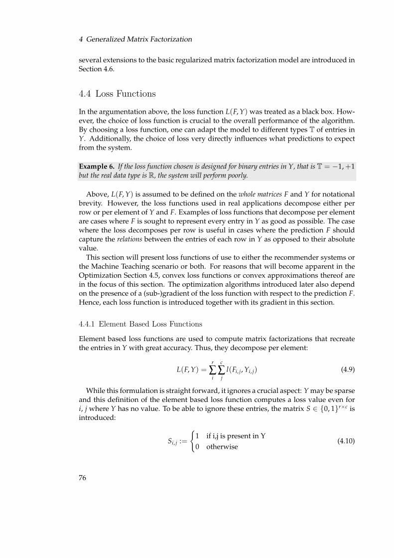
4 Generalized Matrix Factorization
several extensions to the basic regularized matrix factorization model are introduced inSection 4.6.
4.4 Loss Functions
In the argumentation above, the loss function L(F, Y) was treated as a black box. How-ever, the choice of loss function is crucial to the overall performance of the algorithm.By choosing a loss function, one can adapt the model to different types T of entries inY. Additionally, the choice of loss very directly influences what predictions to expectfrom the system.
Example 6. If the loss function chosen is designed for binary entries in Y, that is T = −1, +1but the real data type is R, the system will perform poorly.
Above, L(F, Y) is assumed to be defined on the whole matrices F and Y for notationalbrevity. However, the loss functions used in real applications decompose either perrow or per element of Y and F. Examples of loss functions that decompose per elementare cases where F is sought to represent every entry in Y as good as possible. The casewhere the loss decomposes per row is useful in cases where the prediction F shouldcapture the relations between the entries of each row in Y as opposed to their absolutevalue.
This section will present loss functions of use to either the recommender systems orthe Machine Teaching scenario or both. For reasons that will become apparent in theOptimization Section 4.5, convex loss functions or convex approximations thereof arein the focus of this section. The optimization algorithms introduced later also dependon the presence of a (sub-)gradient of the loss function with respect to the prediction F.Hence, each loss function is introduced together with its gradient in this section.
4.4.1 Element Based Loss Functions
Element based loss functions are used to compute matrix factorizations that recreatethe entries in Y with great accuracy. Thus, they decompose per element:
L(F, Y) =r
∑i
c
∑j
l(Fi, j, Yi, j) (4.9)
While this formulation is straight forward, it ignores a crucial aspect: Y may be sparseand this definition of the element based loss function computes a loss value even fori, j where Y has no value. To be able to ignore these entries, the matrix S ∈ 0, 1r×c isintroduced:
Si, j :=
1 if i,j is present in Y0 otherwise
(4.10)
76

4.4 Loss Functions
This facilitates the following definition of a element based loss function that ignoresentries where Y does not contain a value:
L(F, Y) =r
∑i
c
∑j
Si, jl(Fi, j, Yi, j) (4.11)
As a consequence of this decomposition, the gradient of L(F, Y) with respect to Fdecomposes per element, too:
∂FL(F, Y)i, j = Si, j∂Fi, j l(Fi, j, Yi, j) (4.12)
Given both equation (4.11) and equation (4.12), it is sufficient to describe the actualloss functions in terms of l(Fi, j, Yi, j) and ∂Fi, j l(Fi, j, Yi, j).
Squared Error
The squared error is computed as the squared distance between the true value Yi, j andthe prediction: Fi, j
lsquared(Fi, j, Yi, j) =12
(Fi, j −Yi, j)2 (4.13)
Using this loss results in a regularized least squares regression model. In recom-mender systems, this loss is often used when the entries in Y are ratings. However,ratings are typically not given on a real valued scale but as a one out of n selection. InMachine Teaching, the squared error can be used when the value type of the structureelements is R.
The gradient of the Squared Error with respect to Fi, j can be derived as:
∂Fi, j lsquared(Fi, j, Yi, j) = Fi, j −Yi, j (4.14)
ε-insensitive Regression
In many cases, a prediction Fi, j does not need to be exact but instead needs only to bewithin ε of the exact value. This thought led to the introduction of the ε-insensitive lossfunction as presented in [VGS97]:
lε(Fi, j, Yi, j) = max(0, |Fi, j −Yi, j| −ε) (4.15)
Its gradient can be computed as:
∂Fi, j lε(Fi, j, Yi, j) =
0 |Fi, j −Yi, j| ≤ ε
sign(Fi, j −Yi, j) else(4.16)
Note that this formulation of the loss function is not smooth and that a smooth ap-proximation thereof has been introduced in [DSSS05]. However, the bundle methodoptimizer used here can optimize non-smooth loss functions.
77

4 Generalized Matrix Factorization
Hinge Loss
When dealing with binary data in Y, that is T = −1, +1, the most natural loss to useis the so called zero-one loss:
l01(Fi, j, Yi, j) =
1 Fi, j 6= Yi, j
0 else(4.17)
However, this loss function obviously is not convex in Fi, j as it is piecewise constant.Hence, a convex relaxation of this loss function, the so called Hinge Loss, is commonlyused in machine learning:
lHinge(Fi, j, Yi, j) = max(0, 1− Fi, jYi, j) (4.18)
If the prediction is correct, that is Fi, j = Yi, j, then the product Fi, jYi, j is 1 and the lossvalue is zero. The same is true whenever the sign of Fi, j and Yi, j are equal with theabsolute value of Fi, j ≥ 1, thanks to the max. The loss is effectively unbound for thecase where the sign of Fi, j and Yi, j are not equal. In order to keep the predictions Fi, jwithin T = −1, +1, a prediction rule is used in practice: Whenever Fi, j is less thanzero, the prediction is −1 and else 1.
The resulting function is convex in F and its gradient is computed as:
∂Fi, j lHinge(Fi, j, Yi, j) =
0 Fi, jYi, j ≥ 11 otherwise
(4.19)
Weighted variant: In many real world scenarios, the data set is not balanced betweenthe two classes. In a typical Recommender System, the number of items bought by auser is typically very small compared to the number of items she could buy. In Chap-ter 6, an example from the Machine Teaching scenario will be discussed in depth whichexposes this characteristic.
In that respect, the matrix factorization problem arising has some similarities withthe supervised machine learning from positive and unlabeled data settings addressedin [LL03] and [EN08].
In these cases, it is convenient to attach a weight g to the positive labels. This leadsto the following loss function:
lWHinge(Fi, j, Yi, j) = g(Yi, j) max(0, 1− Fi, jYi, j
)(4.20)
where
g(y) =
g+ y > 01 else
Inclusion of the weight into the gradient computations leads to:
78

4.4 Loss Functions
∂Fi, j lWHinge(Fi, j, Yi, j) =
0 Fi, jYi, j ≥ 1g(Yi, j) otherwise
(4.21)
In [PS09], a solution to a similar problem is proposed based in the work presentedin [HKV08]. However, that solution is limited to the Least Squares loss function.
Logistic Regression
In many instances, one is interested in the probability of a 1 than in its prediction. Forinstance, a Machine Teaching system can only present a limited amount of suggestionsto the learner. The predicted probability can be used to filter that list of predictions andalso provide the learner with a sense of importance of the suggestions.
To predict this probability, one can resort to the logistic regression loss function asintroduced in [CSS00]:
llogistic(Fi, j, Yi, j) = log(1 + exp(−Fi, jYi, j)) (4.22)
Its gradient is computed as:
∂Fi, j llogistic(Fi, j, Yi, j) =−Yi, j
1 + exp(Fi, jYi, j)(4.23)
Weighted variant: The same reasoning presented for the hinge loss can be applied tothe Logistic Regression, too. The
lWlogistic(Fi, j, Yi, j) = g(Yi, j) log(1 + exp(−Fi, jYi, j)) (4.24)
Inclusion of the weight into the gradient computations leads to:
∂Fi, j lWlogistic(Fi, j, Yi, j) =−g(Yi, j)−Yi, j
1 + exp(Fi, jYi, j)(4.25)
4.4.2 Row Based Loss Functions
The loss functions introduced so far compute a loss value per element of the matricesY and F. Optimizing the objective function (4.8) thus yields to predictions in F that aregood on average over all elements. This does not ensure that the predictions are coherentas such, e. g. per row.
However, there are important use cases where per-row coherence is important inthe predictions. Examples include the need to learn inherent per-artifact coherence re-quirements from the data in Machine Teaching. In recommender systems, the need forper-row losses stems from the observation that the output of the recommender systemis often used to compute a ranked list of recommendations for each user.
79
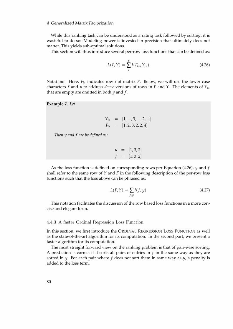
4 Generalized Matrix Factorization
While this ranking task can be understood as a rating task followed by sorting, it iswasteful to do so: Modeling power is invested in precision that ultimately does notmatter. This yields sub-optimal solutions.
This section will thus introduce several per-row loss functions that can be defined as:
L(F, Y) =r
∑i
l(Fi∗, Yi∗) (4.26)
Notation: Here, Fi∗ indicates row i of matrix F. Below, we will use the lower casecharacters f and y to address dense versions of rows in F and Y. The elements of Yi∗that are empty are omitted in both y and f .
Example 7. Let
Yi∗ = [1,−, 3,−, 2,−]Fi∗ = [1, 2, 3, 2, 2, 4]
Then y and f are be defined as:
y = [1, 3, 2]f = [1, 3, 2]
As the loss function is defined on corresponding rows per Equation (4.26), y and fshall refer to the same row of Y and F in the following description of the per-row lossfunctions such that the loss above can be phrased as:
L(F, Y) = ∑f ,y
l( f , y) (4.27)
This notation facilitates the discussion of the row based loss functions in a more con-cise and elegant form.
4.4.3 A faster Ordinal Regression Loss Function
In this section, we first introduce the ORDINAL REGRESSION LOSS FUNCTION as wellas the state-of-the-art algorithm for its computation. In the second part, we present afaster algorithm for its computation.
The most straight forward view on the ranking problem is that of pair-wise sorting:A prediction is correct if it sorts all pairs of entries in f in the same way as they aresorted in y. For each pair where f does not sort them in same way as y, a penalty isadded to the loss term.
80
4.4 Loss Functions
In a more formal way, this loss, which was described in [HGO00] can be described asfollows: For a given pair of entries (u, v) we consider them to be ranked correctly when-ever yu > yv implies that also fu > fv. A loss of is incurred whenever this implicationdoes not hold:
lord( f , y) = ∑yu>yv
C(yu, yv) fu ≤ fv (4.28)
Here C(yu, yv) denotes the cost of confusing an entry of yu with one of value yv and fu ≤ fv is a comparator function:
fu ≤ fv =
1 fu ≤ fv
0 otherwise(4.29)
This comparator function obviously is not convex. Thus, we apply the same softmargin trick as in the hinge loss function introduced in Section 4.4.1:
lord( f , y) = ∑yu>yv
C(yu, yv) max(0, 1− fu + fv). (4.30)
If fu is less or equal than fv, the penalty will be at least 1. If fu is bigger than fv,the penalty will be at most 1 and it vanishes for values of fu that are greater or equalthan fv + 1. Thus, the step in the original comparator fu ≤ fv is replaced by a linearincrease in the loss value around the comparison boundary.
Finally, the value of the loss as defined now is also determined by the number ofentries in y. This clearly is an undesirable property, as the loss value on different rowsof the matrices Y and F is now no longer comparable. Thus, the loss function needs tobe normalized by the number of terms in the sum.
Assume that y is of length m containing m j entries of value j, that is ∑ j m j = m.There are m2 comparisons possible between m entries. However, comparisons betweenentries with equal value don’t fulfill the comparison, hence we need to subtract these∑ j m2
j comparisons. Finally, only half of the comparisons are true. Thus, the number ofterms in the sum can be computed as:
s =12
[m2 −∑
jm2
j
](4.31)
Plugging this constant s into the loss formulation in equation (4.30) yields the follow-ing normalized and convex differentiable ordinal regression loss function:
lord( f , y) =1s ∑
yu>yv
C(yu, yv) max(0, 1− fu + fv). (4.32)
81

4 Generalized Matrix Factorization
Computing the gradient: Each element of f appears as fu and fv in the loss func-tion (4.32). In each case, the loss function is a linear function in this fu or fv. Thisobservation allows us to compute the gradient of the loss function with respect to f ina straight forward fashion:
[∂ f lord( f , y)
]i =
1s
(∑
(yu>yi)∧( fu≤ fi)C(yu, yi)− ∑
(yi>yv)∧( fi≤ fv)C(yi, yv)
)(4.33)
Runtime Performance: Computing the loss involves iterating over all pairs of ele-ments in y and f . Thus, it is a computation of complexity O
(m2), with m being the
length of y. The computation of the gradient, if naively implemented following Equa-tion (4.33), would be a O
(m3) operation, as the computation iterates over all m2 pairs
for all m entries in f . However, both the computation of the loss and the gradient canbe folded into one O
(m2) operation as shown in Algorithm 4.4.3.
Algorithm 1 Computation of the ordinal regression loss lord( f , y) and its gradient∂ f lord( f , y) in O
(m2) time.
input Vectors f and y score matrix Coutput Loss l := l( f , y) and gradient g := ∂ f l( f , y)m = length(y)m j = Number of elements of value j in y
n = 12
[m2 − ∑ j m2
j
]set l := 0set g := 0for i = 1 to m do
for j = 1 to m doif yi < y j ∧ fi ≥ f j then
l = l + Cyi ,y j (1 + fi − f j)gi = gi + Cyi ,y j
g j = g j − Cyi ,y j
end ifend for
end forl = l/ng = g/nreturn l,g
82

4.4 Loss Functions
1 1-1 111
1 1-1 111
1 1-1 111
1 1-1 111
count(1) = 5
count(1) = 4
count(1) = 3
loss += count(1)=3
1 1-1 111 …
Y sorted by F
Figure 4.2: The fast procedure to compute the ordinal regression loss.
Fast Ordinal Regression
In many real world recommender systems, an algorithm that scales quadratic in thenumber of items is unacceptable. These systems often have millions, sometimes hun-dreds of millions of users and in the order of hundreds of thousands of items. Forexample, the subset of the data released by Netflix, a commercial movie rental ser-vice, as part of the Netflix Prize consists of data about more than seventeen thousandmovies and roughly half a million users. When learning to order artifact elements foran instance of the Machine Teaching approach, a quadratic algorithm might be a majorhurdle when delivering real time predictions to the learner.
Therefore, this section presents a novel algorithm to compute the ordinal regressionloss and its gradient that overcomes this limitation. Its time complexity will be shownto scale in O (m log (m)) of the input length y, which presents a major increase in per-formance over the state-of-the-art. First, an intuitive explanation and visualization ofthe main idea of the new algorithm will be given. This is followed by the presentationof the actual algorithm in more formal terms.
Intuition: Given y and f , one can copy y as z. This vector z is then ordered by theorder induced by sorting f . This is can be done in O (m log (m)) time. Additionally,the number of elements with value j in y, denoted my m j can be computed in onelinear sweep over y. Given the results of both of these operations, the loss value can becomputed in a single pass over z my decreasing m j for each visited element in z. Thecounters m j for entries smaller than the current one should all be 0. If not, their sum isadded to the loss value. The main computational cost of this procedure is the sorting off . Thus, the whole process takes O (m log (m)) time.
Figure 4.2 visualizes this intuition for only two possible labels in y, T = −1, 1.First, we compute the number of elements with rating 1 as count(1). Then, in one passover the data, we decrease count(1) if the current value is 1. If it is −1, we know thatthis −1 is part of count(1) wrong orderings in f . Thus, we can increase the loss valueaccordingly. This idea was first presented in [Joa06].
83

4 Generalized Matrix Factorization
Algorithm: This observation is used to form the novel Algorithm 4.4.3. Note thatthe first loop, beginning in line 5, would be sufficient to compute the loss, but not thegradient. It follows from the gradient in Equation (4.33) that each element in f appearstwice in the sums: Once for potentially being too big, and once for being potentially toosmall in each comparison. The second loop, beginning in line 13, thus computes theremaining contributions to the gradient.
The main computational cost stems from line 3, where the argsort of f is computed,a O (m log (m)) operation. The two following loops, are both linear in m and do notchange the complexity of the algorithm. Thus, Algorithm 4.4.3 is of time complexityO (m log (m)).
Algorithm 2 Computation of the ordinal regression loss lord( f , y) and its gradient∂ f lord( f , y) in O (m log m) time
1: input Vectors f and y ∈ 1, ..., z score matrix C2: output Loss l := l( f , y) and gradient g := ∂ f l( f , y)3: Initialize l := 0, g := 0, m := length(y), p := argsort( f )
// Test for items placed too early:4: m j := Number of elements of value j in y5: for i = 1 to m do6: z := yp[i], mz := mz − 17: for k := 1 to z− 1 do8: l := l + mkC(z, k)9: gp[i] := gp[i] + mkC (z, k)
10: end for11: end for
// Test for items placed too late:12: m j := Number of elements of value j in y13: for i := m to 1 do14: z := yp[i], mz =: mz − 115: for k := z + 1 to max(z) do16: gp[i] := gp[i] −mkC (z, k)17: end for18: end for
// Normalization:19: s := 1
2
[m2 − ∑ j m2
j
]20: return l
s , gs
84

4.4 Loss Functions
Conclusion: The presented algorithm presents a significant improvement in run-timecomplexity. Therefore, the use of the logistic regression loss function is now possible inareas where the problem size prohibited to do so before.
4.4.4 An NDCG Loss Function for Matrix Factorization
In many scenarios where a ranking is ultimately sought from the recommender system,ranking measures are used to evaluate the ranking performance of the system, givenknown rankings given by the user. These measures are formed based on an under-standing of what a good ranking is in the specific domain. One common paradigm inthese ranking measures is a weight decay of the ranking importance: Elements rankedhighly are more important than elements ranked low on the final list. This follows theobservation that users are only willing to consider a certain number of items on a listpresented to them and that they scan the list from the top.
In this section, a novel ranking loss function based on one measure, namely the Nor-malized Discounted Cumulative Gain (NDCG) is introduced. First, the measure itselfis described and some important properties are discussed. In the second part of thissection, the conversion of this measure to a loss function as well as a convex upperbound on it will be introduced. Finally, the equations for computing its gradient arederived.
Notation
In order to define this measure, several notations need to be introduced. Throughoutthis section, subscripts (e. g. ai) and array notation (e. g. a[i]) are used interchangeablyto allow for a clear and concise presentation.
Definition 12 (Permutation Vector). A PERMUTATION VECTOR π is a vector which con-tains the indices of another vector, here denoted by a. If the vector a is permuted by π , π [i] isthe index of the element in a that appears at position i after the permutation.
Example 8. πs is a permutation that sorts a decreasingly. Then, the following is true:
a[[πs[i]] ≥ a[πs[i + 1]]∀i ∈ 0 . . . n− 2
aπ shall denote the vector a, permuted by π such that the following is true:
aπ [i] = a[π [i]] ∀a, π
The NDCG measure:
The Normalized Discounted Cumulative Gain (NDCG) is a measure commonly usedin Information Retrieval settings to evaluate the ranking performance of a retrievalsystem [Voo01]. It is appropriate to evaluate recommender systems, too, as the rec-ommender system will retrieve a set of items, given the user as a query. The NDCG
85

4 Generalized Matrix Factorization
∑
44.72 13.65 5.05 1.86 0.56 65.84
Perfect permutation
Contribution to the DCG
∑
10.10 13.65 22.36 1.86 0.56 48.53
First wrong
Contribution to the DCG
∑
44.72 13.65 0.72 1.86 3.91 64.85
Last wrong
Contribution to the DCG
Figure 4.3: Visualization of the sensitivity of DCG to different errors. Note that the“perfect permutation” might not always be obtainable in real data due toties.
formulation is based on the following desirable properties for a performance measurein this context:
• Mistakes at the beginning of the ranked list shall be punished more than those atthe end of the list. More formally, there should be decay of the loss induced overthe length of the list.
• The users of a real system are only willing to consider k items, typically in theorder of 10. Thus, the measure has a cutoff parameter, after which mistakes arenot considered any more.
• The measure shall be independent of the type T of y.
Based on these informal requirements, the DCG and subsequently the NDCG can bedefined:
Definition 13 (DCG). The DISCOUNTED CUMULATIVE GAIN (DCG) with cut-off k isdefined on a sequence y and a permutation π and can be computed as:
DCG(y, k, π) =k−1
∑i=0
2yπ [i] − 1log2(i + 2)
(4.34)
Equation (4.34) is maximized for a permutation πs that sorts y decreasingly. Thedenominator assures that small values at the beginning and large values at the end ofyπ are yielding little gain. The sum in the numerator of Equation (4.34) runs over k andthus removes the influence of elements permuted to positions after k.
86

4.4 Loss Functions
Example 9. Figure 4.3 shows three computations of the DCG. The first row depicts the perfectpermutation. The second row shows that an error in the first half of the permutation has astronger influence on the outcome as the error shown in the last row that occurred in the secondhalf of the permuted list.
However, the formulation of the DCG is not invariant to scaling y. In fact, DCG(l ∗y, k, π) = l ∗ DCG(y, k, π). Thus, predictions for users who prefer to rate items highlywill be evaluated better than those who rate items using lower labels. To overcome this,the Normalized DCG (NDCG) is introduced:
Definition 14. The NORMALIZED DISCOUNTED CUMULATIVE GAIN (NDCG) of a vectory, permutation π and cutoff k is defined as:
NDCG(y, k, π) =DCG(y, k, π)DCG(y, k, πs)
(4.35)
where πs is the permutation which sorts Y decreasingly.
The NDCG is maximized for the permutation π that sorts y decreasingly. Addition-ally, the NDCG is bounded between 0.0 and 1.0. Thus, the NDCG fulfills the last of thedesirable properties outlined above.
Construction of a convex loss function for NDCG
The remainder of this section shows how to derive a convex differentiable loss functionfrom the NDCG in Equation (4.35). This derivation draws inspiration from [TJHA05,TGK04] and is presented in the following steps:
1. Conversion of the gain NDCG into a loss.
2. Construction of a convex upper bound on the so-found loss function.
Finally, it is shown how to compute the loss function value and its gradient by reduc-ing it to a linear assignment problem.
Step 1: Loss conversion
To convert the gain function in Equation (4.35) into a loss function, we rely on the factthat it is bounded from above by 1.0. Thus, the loss function for NDCG for a givencutoff k can be defined as:
∆(π , y) = 1− NDCG(y, k, π) (4.36)
This loss function assumes the value of 0 for the permutation πs that sorts y decreas-ingly. Note that this function is not convex in π . In fact, it is piecewise constant.
87

4 Generalized Matrix Factorization
Step 2: Derivation of the upper bound
Definition 15. Let c be a decreasingly sorted, non-negative vector and f be the prediction.Then we define:
l( f , y, π) = maxπ
[∆(π , y) + 〈c, fπ − f 〉] (4.37)
It will now be shown that l( f , y, π) as defined in Equation (4.37) is a convex upperbound on ∆(π , y) (4.36).
Lemma 1. The function (4.37) is convex in f and an upper bound to the loss function (4.36).
Proof. The proof is done in two phases. First, the convexity of (4.37) in f is shown.Second, the fact that (4.37) is an upper bound to (4.36) is proven.
Convexity: The argument of the maximization over the permutations π is linear andthus a convex function in f . Taking the maximum over a set of convex functionsis convex itself, which proves the first claim.
Upper Bound: In order to proof that (4.37) is an upper bound to (4.36), we apply theinsight that the inner product between two vectors is maximized if both vectorsare sorted by the same criterion.
Let π∗ := argsort(− f ) be the ranking induced by f and c be a decreasinglysorted, non negative vector. To see that it is an upper bound, we use the factthat
l( f , y) ≥ ∆(π∗, y) + 〈c, fπ∗ − f 〉 ≥ ∆(π∗, y). (4.38)
The second inequality follows from the fact that π∗ maximizes 〈c, fπ∗〉 by thePolya-Littlewood-Hardy inequality.
Thus, it can be concluded that (4.37) is convex in f and an upper bound to the lossfunction (4.36), which proofs the claim.
Step 3: Derivation of the gradient
For optimization purposes, the gradient of l( f , y, π) with respect to f needs to be de-rived. The fist step in this derivation is based upon the fact that the gradient is definedon the maximizer π of l( f , y, π):
∂ f l( f , y, π) = ∂ f maxπ
[∆(π , y) + 〈c, fπ − f 〉]
= ∂ f 〈c, fπ − f 〉+ ∂ f ∆(π , y)= ∂ f 〈c, fπ − f 〉+ 0= ∂ f 〈c, fπ − f 〉
88

4.4 Loss Functions
The sum in the inner product can be decomposed, leaving us with:
∂ f 〈c, fπ − f 〉 = ∂ f 〈c, fπ 〉 − ∂ f 〈c, f 〉= ∂ f 〈c, fπ 〉 − c
To solve the gradient ∂ f 〈c, fπ 〉, we use the insight that 〈a, bπ 〉 = 〈aπ−1 , b〉, where π−1
denotes the inverse permutation to π :
∂ f 〈c, fπ − f 〉 = ∂ f 〈cπ−1 , f 〉 − c= cπ−1 − c
Therefore, we can compute the final gradient as:
∂ f l( f , y, π) = cπ−1 − c (4.39)
Computation of the loss
Computing the value of the loss function (4.37) and its gradient (4.39) is a challenge,as the maximizing permutation π is needed which in worst case may mean that allpossible permutations have to be considered. Below, it is shown that the solution forthis maximization can be found by solving a linear assignment problem with a costmatrix specific to this problem.
Lemma 2. The solution of Equation (4.37) can be found by solving the following linear assign-ment problem:
min ∑i
∑j
Ci, j ∗ Xi, j
subject to:
∑i
Xi, j = 1 ∀ j
∑j
Xi, j = 1 ∀i
Xi, j ≥ 0 ∀i, j
with a cost matrix:
Ci, j = κi2y[ j] − 1
DCG(y, k, πs)log2(i + 2)− ci f j
The solution to the linear assignment problem is integral, as the constraint matrix X is totallyunimodular. This means that Xi, j is either 1 or 0 for all i, j. Thus, we can transform the solutionX back into a permutation π by setting π [i] = the j for which Xi, j is 1. This π is the solutionto Equation (4.37).
89

4 Generalized Matrix Factorization
Proof. Recall
l( f , y, π) = maxπ
[∆(π , y) + 〈c, fπ − f 〉] (4.40)
where ∆(π , y) = 1− NDCG(y, k, π) for some arbitrary but fixed k. f is the currentprediction and fπ is the current prediction permuted by π . Using this notation, thefollowing derivations are possible:
l( f , y, π) = maxπ
[1− NDCG(y, k, π) + 〈c, fπ − f 〉]
= maxπ
[〈c, fπ − f 〉 − NDCG(y, k, π)] + 1
= maxπ
[〈c, fπ 〉 − NDCG(y, k, π)] + 1− 〈c, f 〉
= maxπ
[〈c, fπ 〉 −
DCG(y, k, π)DCG(y, k, πs)
]+ 1− 〈c, f 〉
The π which maximizes this equation also maximizes the following one, as 1− 〈c, f 〉are independent of π :
maxπ
[〈c, fπ 〉 −
DCG(y, k, π)DCG(y, k, πs)
]= max
π
[〈c, fπ 〉 −
1DCG(y, k, πs)
k−1
∑i=0
2y[π [i]] − 1log2(i + 2)
]
= maxπ
[〈c, fπ 〉 −
k−1
∑i=0
1DCG(y, k, πs)
2y[π [i]] − 1log2(i + 2)
]
= maxπ
[〈c, fπ 〉 −
2y[π [i]] − 1DCG(y, k, πs)log2(i + 2)
]
Defining
Xi, j =
1 if π [i] = j,0 otherwise
and κi =
1 if i < k,0 otherwise
allows us the following reformulation:
90

4.4 Loss Functions
maxπ
[〈c, fπ 〉 −
k−1
∑i=0
2y[π [i]] − 1DCG(y, k, πs)log2(i + 2)
]
= maxX
[∑
i∑
jci f jXi, j −∑
j
k−1
∑i=0
Xi, j2y[ j] − 1
DCG(y, k, πs)log2(i + 2)
]
= maxX
[∑
i∑
jci f jXi, j −∑
i∑
jκi
Xi, j(2y[ j] − 1)DCG(y, k, πs)log2(i + 2)
]
= maxX
[∑
i∑
jci f jXi, j −κi
Xi, j(2y[ j] − 1)DCG(y, k, πs)log2(i + 2)
]
= maxX
[∑
i∑
jXi, j(ci f j −κi
2y[ j] − 1DCG(y, k, πs)log2(i + 2)
]
Thus, the problem can be solved using the following linear assignment problem for-mulation:
min ∑i
∑j
Ci, j ∗ Xi, j
subject to:
∑i
Xi, j = 1 ∀ j
∑j
Xi, j = 1 ∀i
Xi, j ≥ 0 ∀i, j
with:
Ci, j = −(
ci f j −κi2y[ j] − 1
DCG(y, k, πs)log2(i + 2)
)
= κi2y[ j] − 1
DCG(y, k, πs)log2(i + 2)− ci f j
The solution to this linear assignment problem is integral, Xi, j is either 1 or 0 for alli, j. Thus, we can transform the solution X back into a permutation π by setting π [i] =the j for which Xi, j is 1. Using this permutationπ , the value of Equation (4.37) can becomputed, which proofs the claim.
91

4 Generalized Matrix Factorization
4.4.5 Conclusion
In this section, we presented several choices regarding the loss function to be used.In addition to transferring some well-known element based loss functions from su-pervised machine learning to matrix factorization, we introduced the concept of rowbased loss functions. Two loss functions have been discussed in this context: We de-rived a faster algorithm for the computation of the ordinal regression loss function anddeveloped a loss function which can be used to directly optimize the prediction for theNDCG evaluation measure.
We did not yet, however, present how to actually optimize the objective function (4.8).The next section presents an optimization procedure to do so.
4.5 Optimization
Now that suitable choices for the loss function have been discussed, the only part of aworking matrix factorization algorithm which we did not present yet is the optimiza-tion procedure used to minimize the objective function (4.8).
This procedure is described in this section. As briefly mentioned when introducingthe loss functions above, we assume the loss function to be convex and differentiablein f , or at least sub-differentiable. However, this assumption does not guarantee thatthe objective function (4.8) is jointly convex in C and R. In fact, the contrary is true:Equation (4.8) is not jointly convex in C and R:
Lemma 3. Equation (4.8) is not guaranteed to be jointly convex in C and R.
Proof. Let us assume a very simple case of Matrix Factorization: C, R ∈ R1 and the leastsquares loss function. Then, the loss function becomes:
L(F, Y) = ((F)−Y)2 = (RC>)2 − 2RC>Y + Y2
A function is convex if its hessian is positive semi-definite. The hessian of this losscan be computed based on the following partial derivatives:
LU(F, Y) = 2RC>2 − 2C>YLM(F, Y) = 2R2C> − 2RY
LUU(F, Y) = 2C>2
LMM(F, Y) = 2R2
LUM(F, Y) = 4RC> − 2YLMU(F, Y) = 4RC> − 2Y
This leads to the following hessian:
H = 2(
C>2 2RC> −Y2RC> −Y R2
)
92
4.5 Optimization
If H is were semi-definite, the function L was jointly convex in R and C. A matrix ispositive semi-definite if its determinant is positive. However, the determinant of H is:
det(H) = 2(C>2R2 − (2RC> −Y)2)= 2(C>2R2 − 4R2C>2 + 4RC>Y−Y2)= 2(−3R2C>2 + 4RC>Y−Y2)= 8RC>Y− 6R2C>2 − 2Y2
It is easy to see that for every fixed Y, there will be R and C such that 6R2C>2 willbe bigger than 8RC>Y which renders the determinant negative. Thus, the objectivefunction (4.8) is not guaranteed to be jointly convex in R and C for a simple specialcase, which proofs the claim.
Efficient optimization of non-convex functions is challenging and multiple differ-ent approaches such as Stochastic Gradient Descent [Bot04], Semi-Definite Program-ming [SRJ05] and Subspace Gradient Descent [RS05] have been proposed to find thesolution for factor models. Semi-Definite Programming as described in [RS05] is theo-retically the most elegant solution, as it is guaranteed to find a globally optimal solu-tion. However, the computational requirements of doing so a prohibitive for all but thesmallest problems.
The Stochastic Gradient Descent methods are computationally elegant as they canbe implemented in an online algorithm that optimizes in multiple linear sweeps overthe data. However, they are based on the assumption of a per-element loss functionwhich, for the reasons outlined above, is not desirable in the Machine Teaching andsome important Recommender Systems scenarios.
Thus, an algorithm based on Subspace Gradient Descent is presented here. The keyinsight behind Subspace Gradient Descent is the fact that the objective function (4.8) isconvex in C if R is kept fixed and convex in R if C is kept fixed. Thus, we can optimizeby alternating between optimization steps over R and C as shown in Algorithm 3.
Algorithm 3 Alternate Subspace Descent for Matrix FactorizationInitialize R and C randomlyrepeat
For fixed C minimize (4.8) with respect to R.For fixed R minimize (4.8) with respect to C.
until no more progress is made or a maximum iteration count is reached.
Note that as the overall optimization problem is still non-convex this procedure can-not be guaranteed to converge to a global optimum. However, experimental evalu-ations show that an implementation of this procedure consistently finds solutions ofequal quality, if not the same solution when minimizing the objective function on thesame data set but different random initializations of R and C.
93
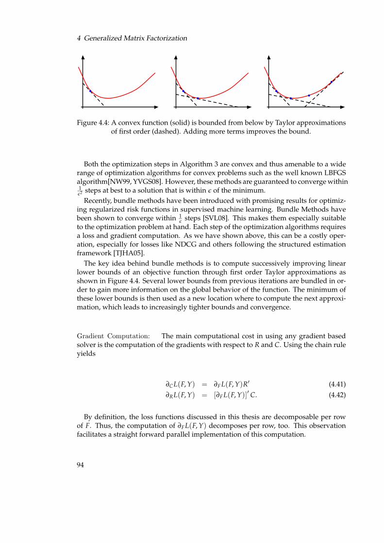
4 Generalized Matrix Factorization
Figure 4.4: A convex function (solid) is bounded from below by Taylor approximationsof first order (dashed). Adding more terms improves the bound.
Both the optimization steps in Algorithm 3 are convex and thus amenable to a widerange of optimization algorithms for convex problems such as the well known LBFGSalgorithm[NW99, YVGS08]. However, these methods are guaranteed to converge within1ε2 steps at best to a solution that is within ε of the minimum.
Recently, bundle methods have been introduced with promising results for optimiz-ing regularized risk functions in supervised machine learning. Bundle Methods havebeen shown to converge within 1
εsteps [SVL08]. This makes them especially suitable
to the optimization problem at hand. Each step of the optimization algorithms requiresa loss and gradient computation. As we have shown above, this can be a costly oper-ation, especially for losses like NDCG and others following the structured estimationframework [TJHA05].
The key idea behind bundle methods is to compute successively improving linearlower bounds of an objective function through first order Taylor approximations asshown in Figure 4.4. Several lower bounds from previous iterations are bundled in or-der to gain more information on the global behavior of the function. The minimum ofthese lower bounds is then used as a new location where to compute the next approxi-mation, which leads to increasingly tighter bounds and convergence.
Gradient Computation: The main computational cost in using any gradient basedsolver is the computation of the gradients with respect to R and C. Using the chain ruleyields
∂CL(F, Y) = ∂FL(F, Y)R′ (4.41)∂RL(F, Y) = [∂FL(F, Y)]′ C. (4.42)
By definition, the loss functions discussed in this thesis are decomposable per rowof F. Thus, the computation of ∂FL(F, Y) decomposes per row, too. This observationfacilitates a straight forward parallel implementation of this computation.
94

4.5 Optimization
4.5.1 Optimization over the Row Matrix R
The same observation can be applied to the optimization of (4.8) over R for a fixed C.Not only does the loss function decompose per row, but so does the Frobenius normused as the regularizer. Thus, the optimization over R decomposes into r convex opti-mization problems, one per row of Y and F. This observation is used in Algorithm 4 toform an efficient optimization procedure for the first step in Algorithm 3, the optimiza-tion over R. Note that in fact, each of the per-row optimization problems is a standardregularized risk minimization problem as discussed in the supervised machine learn-ing literature. Example: When choosing the Hinge loss function, the problem is exactlythat of a linear support vector machine.
Algorithm 4 Optimization over R with fixed Cinput Parameter matrices R and C, data matrix Youtput Matrix Rfor i = 1 to r do
Select idx as the nonzero set of Yi∗Initialize w = Ri∗Ri,idx = argminw l(wCidx,∗, Yi,idx) + λr
2 ‖w‖2
end for
4.5.2 Optimization over the Row Matrix C
The optimization over C is not amenable to the same treatment, as the loss function,by design, does not decompose per column of Y and F. Thus, the complete gradientand loss over C needs to be computed. As introduced earlier, the computations of theloss value and its gradient with respect to F can still be decomposed per row. The maincomputational bottleneck then becomes the final multiplication to compute:
∂CL(F, Y) = R′∂FL(F, Y) (4.43)
This formulation, if implemented naively, poses a serious challenge regarding thememory consumption. Recall that ∂FL(F, Y) is of the same size of F and that the lat-ter is never constructed in memory, as it is too large in many Recommender Systemsinstances which have millions of rows (users) and thousands of columns (items). There-fore, the construction of ∂FL(F, Y) in memory should also be avoided.
However, special care can be taken when implementing this multiplication to re-duce the memory consumption of this procedure by iteratively computing the entriesof ∂CL(F, Y) in one pass over all rows of F and Y. Algorithm 5 is build upon this notion.
95

4 Generalized Matrix Factorization
Algorithm 5 Efficient computation of ∂CLinput Parameter matrices R and C, data matrix Youtput Gradient of the loss function L w.r.t C: ∂CLinitialize with 0: ∂CL← 0c×d
for i = 1 to r doFind index idx where Yi∗ 6= 0D← ∂FL(Ri∗C′idx,∗, Yi,idx)∂CL← ∂CL + R′D
end forreturn ∂CL
4.5.3 New Row Optimization
In many scenarios, the system needs to react to new lines in Y. In Recommender Sys-tems, these new lines correspond to new users joining the system. In Machine Teaching,new lines in Y are the default case: Each new line in Y corresponds to a new, partiallyfinished artifact. The system is then asked to perform predictions on this partial artifactto support the learner.
For a large number of rows present in Y, one more is likely to have little influence onC. Additionally, the optimization with respect to R decomposes per row of Y. Theseobservations enable minimizing the objective function (4.8) with respect to this one newrow in Y for a fixed C in order to obtain a new row in R and thus a prediction for thisnew row.
Note that this is similar to the regularized risk minimization formulation of super-vised machine learning. The main difference is that the known features of the super-vised scenario, typically denoted by X, are replaced here with the learned features of thecolumns contained in C.
4.6 Extensions to the Regularized Matrix Factorization Model
Given the previous sections, a matrix factorization model can be constructed for manyMachine Teaching and Recommender Systems scenarios. In this section, several exten-sions to this model are introduced that facilitate better prediction performance. It is alsodiscussed how to integrate these extensions to the optimization procedure described inSection 4.5.
4.6.1 Row and Column Biases
Each row and each column of Y may carry an individual bias. In Recommender Sys-tems, this bias may be the result of the individual user’s rating habits for the rows.The columns may be biased by a universal quality associated with a certain item. Forinstance, ’Plan 9 from Outer Space’ will probably not attract lots of high ratings whileother movies may prove universally popular. Similar biases are conceivable in Machine
96

4.6 Extensions to the Regularized Matrix Factorization Model
Teaching scenarios where a certain structure element value almost always is around aspecific value. That value may then be used as the offset in the sense of this extension.
Biases like this can be introduced into the model by expanding the prediction func-tion from Equation (4.1) with two more terms: The row bias ri and the column bias c j:This can be taken into account by means of an offset per movie. This can be incorpo-rated via
Fi, j =⟨
Ri∗, C j∗⟩
+ ri + c j. (4.44)
Incorporation of these bias terms into the optimization procedure is done by extend-ing R and C by two columns each: One for the bias vector, and one with a constantvalue of 1.
In this form no algorithmic modification for the R and C optimization is needed. Thecomputational cost of this extension can be neglected, as the number of factors d isincreased by only 2.
Note that this offset is different from a simple normalization of the input data andis not meant to replace pre-processing procedures altogether. The offset is learned forthe loss function in use and for each row and column, while it would be tricky to find anormalization that does cater for both appropriately at the same time.
4.6.2 Adaptive Regularization
In many cases, the rows and columns of Y are not evenly filled. In a movie recom-mender scenario, some users rated thousands of movies while others only a few. Thus,a universal regularization parameter for all these rows is not advisable, as rows withmany entries should be allowed a more ’complicated’ model than those with only afew. The same argument holds for the columns in Y. For example in a Coding MachineTeaching System where some methods are universally popular and thus get called of-ten.
Those issues can be dealt with by sample-size adaptive regularization for both columnsand rows. Denote by Dr and Dc diagonal matrices corresponding to rows and columnsof Y. Setting Dr
ii = n−αi and Dr
j j = m−αj where ni denotes the number of entries in row i
and m j denotes the number of entries in column j, we obtain a sample size dependentregularizer as follows:
minU,M
L(F, Y) +λc
2tr C>DcC +
λr
2tr R>DrR.
In our experiments (reported in Chapter 5) we found that α = 0.5 provides bestgeneralization performance. This is equivalent to the regularization scales provided ina maximum a posteriori setting where the log-prior is fixed whereas the evidence scaleslinearly with the number of observations.
As the computation for this scaling can be done in advance, the computational costof the adaptive regularizer is not significant when compared to the overall run time.The needed statistics can even be pre-computed and reused in many experiments.
97

4 Generalized Matrix Factorization
4.6.3 Structure Exploitation with a Graph Kernel
In many instances, the sheer presence of an entry in the matrix Y carries importantinformation in addition to the actual value stored at that point in Y, e. g. in the movierecommender domain. The fact that a user bothered to watch and subsequently rate amovie is an important piece of information that is genuinely distinct from the numericalvalue of the rating given. After all, renting, watching and labeling a movie representsa substantial effort, which the user presumably only invests into movies she is likely tolike.
Example 10. Knowing that a user rated ’Die Hard’, ’Die Hard 2’, and ’Top Gun’ makes itlikely that this user is interested in action movies.
One would expect that we should be able to take advantage of this structural infor-mation in addition to the actual scores. One possibility, proposed in [BH04] is to usethe inner product between two rows of Y as a kernel for comparing two different rows.In this case they define the kernel between the rows i and i′ to be 〈Si∗, Si′∗〉. It is wellknown that such a model is equivalent to using a linear model with row-features givenby S.
The main drawback of this approach is that one needs to compute this kernel functionbetween all users which scales quadratic in their number. Instead, one can use anotherformulation which uses the same insight, the importance of the binary aspects of Yin a computationally more efficient framework. To do so, we introduce an additionalparameter matrix A ∈ Rc×d to replace R with R + SA, which leads to the followingprediction function:
F = (R + SA) C> = RC> + SAC> (4.45)
In this formulation, A controls a mixture of column features to be assigned to eachrow. In the movie recommender example above, every user now partially assumesfeatures of the movie she watched based on the mixing coefficients stored in A. Or, inother words, the proposed solution is based upon the assumption that “we are whatwe watch” up to a level encoded in A. We can optimize over A in a straight-forwardmanner by introducing a third step into the subspace descent described in Algorithm 3.
A similar approach has been proposed in [SM08], whereas a row-normalized ver-sion of S is used. In [WKS08c], it has been shown that all three approaches (the onepresented here, the one in [SM08] and the one in [BH04]) are in fact equivalent.
4.6.4 Row and Column Features
Depending on the application scenario, features of both the rows and the columns maybe available. In a Recommender System, demographic information is often knownabout the users and the items can be described by a set of features, too. In [ABEV06],the integration of features is proposed by defining a kernel between rows and columnsthat integrates features. Another way of introducing features is to use them as a priorfor the factors, as studied in [AC09].
98

4.7 Conclusion
Here, we present a integration of features to our matrix factorization framework byadding several linear supervised learning models: Following common supervised ma-chine learning notation, the rows of XR ∈ Rr×dR shall contain the dR feature vectors forthe rows of Y. The rows of XC ∈ Rc×dC contain those dC features of the columns of Y.
Using these two new matrices, the prediction function from Equation (4.1) can beextended to use column features:
Fi, j =⟨
Ri∗, C j∗⟩
+⟨
WRi∗, XC
j∗
⟩(4.46)
Here, WR ∈ Rr×dC is a matrix whose rows are the weight vectors for the columnfeatures per row. The very same idea can be applied to row features as well:
Fi, j =⟨
Ri∗, C j∗⟩
+⟨
WRi∗, XC
j∗
⟩+⟨
WCi∗, XR
j∗
⟩(4.47)
The matrix WM ∈ Rc×dU encodes the weight vector for each column.As with the offsets, the features can be integrated into the algorithmic procedure
described above without any changes. To do so, one would extend C with the featuresfrom XC, R with the features from XR. These new entries are masked from optimizationand regularization such that their value stays fixed.
To learn the parameters, R is extended by WR and C by WC. The optimization over Rand C includes these new entries. This yields the parameter vectors WR and WC. Pleasenote that the Frobenius norm decomposes per entry in R and C. Thus, the newly in-troduced parameters are regularized as if there would be a L2 norm imposed on them.This essentially recovers a regularized risk minimization problem for these weight vec-tors.
4.7 Conclusion
In this chapter, a generalized matrix factorization model and algorithm has been pre-sented. As shown at the beginning of this chapter (Section 4.1 on page 70), the modelunderlying this approach can be applied both to recommender systems and MachineTeaching applications. The presented approach is a generalization of the state-of-the-artin several respects.
Regularizer: While this thesis focuses on the Frobenius norm as the model regularizer,many more choices such as the L1-norm are possible without leaving the frame-work presented here. The adaptive regularization can be applied to a wide rangeof regularizers, too.
Loss Functions: The model and algorithm here can be used with a wide range of lossfunctions known in the supervised machine learning community.
Especially notable is the possibility to use non-smooth loss functions due to theuse of the bundle method solver. Even more so, the applicability of matrix factor-ization to per-row loss functions is a major contribution as it facilitates the opti-mization of ranking losses in recommender systems. To this end, one novel loss
99

4 Generalized Matrix Factorization
function to directly optimize for the NDCG score and a substantially faster ver-sion of the ordinal regression loss function have been presented. Per-row lossesalso are a crucial ingredient in making matrix factorization a viable method for alarge class of Machine Teaching systems.
Hybrid Approach: The inclusion of features as described above extends matrix factor-ization to be what is known as a “hybrid recommender system”: One that can useboth the collaborative effect of users interacting on the same set of items as well asexplicitly known features of the users and items. This is an important step in ad-dressing the new user problem, which, as we have shown earlier, arises naturallyin Machine Teaching.
The graph kernel and the adaptive regularization make it possible to use additionalknowledge embodied in the rating matrix or the matrix representation of an artifact inthe Machine Teaching setting.
The approach presented in this chapter provides a solid base for the construction ofMachine Teaching systems for detailed feedback, as the prediction of suggestions for anew or changed artifact is fast and, as shall be shown below, very accurate. The widerange of possible loss functions allow the system to be used in a multitude of MachineTeaching scenarios and the possibility to use features of the artifact or the structuralelements thereof can further increase this performance.
Next steps in this thesis: Before applying the algorithm in a Detailed Feedback Ma-chine Teaching approach in Chapter 6, we first evaluate it on well established Recom-mender Systems data sets to compare its performance to the state-of-the-art in that fieldin Chapter 5.
100

5 Evaluation on Recommender Systems Data
Contents5.1 Evaluation Setup . . . . . . . . . . . . . . . . . . . . . . . . . . . . . . . 102
5.1.1 Evaluation Measures . . . . . . . . . . . . . . . . . . . . . . . . . 1025.1.2 Evaluation Procedure . . . . . . . . . . . . . . . . . . . . . . . . 1035.1.3 Data Sets . . . . . . . . . . . . . . . . . . . . . . . . . . . . . . . . 104
5.2 Results and Discussion . . . . . . . . . . . . . . . . . . . . . . . . . . . 1055.2.1 Model Extensions . . . . . . . . . . . . . . . . . . . . . . . . . . . 1055.2.2 Ranking Losses . . . . . . . . . . . . . . . . . . . . . . . . . . . . 106
5.3 Conclusion . . . . . . . . . . . . . . . . . . . . . . . . . . . . . . . . . . 109
101

5 Evaluation on Recommender Systems Data
5.1 Evaluation Setup
This chapter presents empirical evaluation results of the algorithm discussed so farin the Recommender Systems scenario before moving on to the application of the al-gorithm to a Detailed Feedback Machine Learning example in the next chapter. Thereason for evaluating on Recommender Systems data lies in the fact that this field ofresearch is well established:
• Data sets are readily available.
• The evaluation method including the evaluation measure is widely agreed uponin the field.
• Thus, it is possible to assess the performance of an algorithm in comparison to therelated work.
Obviously, none of this is true for the Machine Teaching area. The purpose of theevaluation presented in this chapter therefore is to assure the general performance ofthe algorithm before depending upon both – the algorithm and its performance – insubsequent steps.
Similar to the evaluation presented in Chapter 3, the evaluation is discussed in twosteps: First, the evaluation method including the used measures and the data and thepre-processing thereof are introduced. The remainder of this chapter then presentsempirical results and their discussion for the two main questions to be evaluated:
1. Do the model extensions proposed in Section 4.6 add to the performance of theRecommender System?
2. Do the per-row losses improve the ranking performance of the system?
5.1.1 Evaluation Measures
In order to evaluate the predictive performance of the different variants of the model –rating and ranking prediction – we resort to two evaluation measures.
Rating Performance: Following the majority of the literature, the rating performanceis evaluated with the root mean squared error (RMSE) measure:
RMSE(F, Y) =1
2n
r
∑i=0
c
∑j=0
Si, j(Fi, j −Yi, j)2 (5.1)
Where the binary matrix S indicates whether or not a user rated an item:
Si, j =
1 if user i rated item j0 otherwise
102

5.1 Evaluation Setup
and n is the number of those ratings in Y, e.g.:
n =r
∑i=0
c
∑j=0
Si, j
Ranking Performance: In order to evaluate the ranking performance of the system, weresort to the Normalized Discounted Cumulative Gain (NDCG) measure as introduced inSection 4.4.4. The NDCG of a vector y, permutation π and cutoff k is defined as:
NDCG(y, k, π) =DCG(y, k, π)DCG(y, k, πs)
(5.2)
The permutation π is computed as the argsort of the predicted values: π = argsort( f ).The perfect permutation πs is the argsort of the true ratings given by the user: πs =argsort(y). A NDCG of 1.0 indicates that the model sorts the items in the same order asthe user. The parameter k is a cut-off beyond which the actual ranking does no longermatter. This follows the intuition that typical recommender systems can only present alimited amount of items to the user. In all our experiments, we evaluated using k = 10,which is commonly referred to as NDCG@10. We report the average NDCG@10 overall users below.
5.1.2 Evaluation Procedure
We distinguish two different evaluation scenarios: strong and weak generalization.
Weak generalization: This is the scenario commonly discussed in the literature: Foreach user, a number n of ratings is sampled from the known data. The system isthen trained on these ratings and evaluated on the remaining items. We presentresults for n = 10, 20, 50. This evaluation resembles a system with an establisheduser base that recommendations are generated for.
Strong generalization: As discussed earlier, the Machine Teaching scenario is depen-dent on fast and accurate solutions to what is referred to as the new user problemin Recommender Systems research: Given a fully trained model, predict for a userthat was not part of the initial training phase of the system.
To simulate this scenario, we follow the procedure suggested in [YYTK06]: Movieswith less than 50 ratings are discarded. The 100 users with the most rated moviesare selected as the test set and the methods are trained on the remaining users. Inevaluation, 10, 20 or 50 ratings are sampled from the test users. We then use theseratings to learn a new user feature matrix Rstrong by performing a single iterationof the optimization over R as described in Section 4.5.3. The remaining ratingsare used as the test set.
Note that sampling a small number of ratings for the training set mimics a real worldrecommender setting where ratings are very scarce compared to the total number ofmovies.
103

5 Evaluation on Recommender Systems Data
Data set Users Movies Ratings Rating ScaleMovieLens 983 1682 100000 1-5 StarsEachMovie 61265 1623 2811717 1-6 Stars
Netflix 480189 17770 100480507 1-5 Stars
Table 5.1: Data set statistics
In all experiments, the regularization parameters λr and λc were fixed and not for-mally tuned. The dimension of R and C was set to d = 10 for the evaluation of theextensions and to d = 100 for the evaluation of the different losses. We did not observesignificant performance fluctuations when comparing the performance of the systemusing d = 30 in [SM08]. This is an interesting observation in its own right: The prefer-ences of a user for movies can be described by a relatively small number (in the orderof 10) of factors.
All experiments were performed ten times with different random draws of the trainand test set from the data sets. In total, we report results from more than 5000 experi-ments.
5.1.3 Data Sets
Evaluations have been conducted on three data sets that are well known in the recom-mender systems literature:
MovieLens: The MovieLens data stems from the research movie recommender of thesame name1 of the GroupLens research group2 in the Department of ComputerScience and Engineering at the University of Minnesota.
EachMovie: EachMovie was a recommender run by HP/Compaq Research (formerlyDEC Research). The data set became available when the recommender was shutdown and it has since been used in numerous recommender systems publications.However, the data set was retired in October 2004 and is since no longer availablefor download.
Netflix: The Netflix data set was collected and published by the online movie rentalservice Netflix3 as part of their Netflix Prize challenge4.
The data sets are of very different sizes, their descriptive statistics can be found intable 5.1.
1http://movielens.umn.edu/2http://www.grouplens.org/3http://netflix.com4http://www.netflixprize.com/
104

5.2 Results and Discussion
Method N=10 N=20 N=50EachMovie Plain 0.625± 0.000 0.639± 0.000 0.641± 0.000
Offset 0.646± 0.000 0.653± 0.000 0.647± 0.000GraphKernel 0.583± 0.000 0.585± 0.000 0.590± 0.001OffsetGK 0.576± 0.000 0.597± 0.000 0.580± 0.001
MovieLens Plain 0.657± 0.000 0.658± 0.000 0.686± 0.000Offset 0.678± 0.000 0.680± 0.000 0.701± 0.000GraphKernel 0.624± 0.001 0.644± 0.000 0.682± 0.000OffsetGK 0.670± 0.001 0.681± 0.000 0.682± 0.000
Table 5.2: The NGDC@10 accuracy over ten runs and the standard deviation for theweak generalization evaluation.
Method N=10 N=20 N=50EachMovie Plain 0.859± 0.000 0.731± 0.000 0.627± 0.000
Offset 0.859± 0.000 0.734± 0.000 0.631± 0.000GraphKernel 0.837± 0.000 0.693± 0.000 0.553± 0.001OffsetGK 0.832± 0.000 0.689± 0.000 0.587± 0.001All 0.836± 0.000 0.702± 0.000 0.585± 0.000
MovieLens Plain 0.875± 0.000 0.750± 0.000 0.673± 0.000Offset 0.886± 0.000 0.764± 0.000 0.703± 0.001GraphKernel 0.845± 0.000 0.720± 0.001 0.667± 0.000OffsetGK 0.882± 0.000 0.773± 0.000 0.703± 0.000All 0.869± 0.000 0.730± 0.002 0.645± 0.005
Table 5.3: The NGDC@10 accuracy over ten runs and the standard deviation for theinverted weak generalization evaluation.
5.2 Results and Discussion
5.2.1 Model Extensions
To evaluate the model extensions, we performed experiments for each combination ofthe extensions as it cannot be guaranteed that the combination of all extensions per-forms best. As we are interested in the performance of the extensions, all experimentsare done with a single loss function, namely the least squares loss.
Weak generalization: Table 5.2 contains the results of the weak generalization scenarioexperiments. We observe that adding the offset terms yields significant improve-ments in the performance of the model. On the other hand, enabling the GraphKernel does not significantly improve performance. This can be attributed to thefact that the regularization factors were not tuned. Enabling the Graph Kerneladds a large set of additional parameters to the model which might lead to over-
105

5 Evaluation on Recommender Systems Data
fitting without the adjustment of the regularization parameters. Nonetheless, theGraph Kernel did add further improvements together with the offsets.
Inverted weak generalization: Note that due to the weak generalization proceduredefinition, the adaptive regularization extension cannot have an influence, as allexperiments are done on 10, 20 or 50 movies per user. Thus, we use the same dataset split reversed for evaluating the adaptive regularizer: For each user, 10, 20 or50 movies are used as the test set, with all the remaining movies being the trainingset.
The results of this set of experiments can be found in Table 5.3. They again confirmour observations in the previous setting. The offset term combined with the graphkernel brings significant performance gains.
Strong generalization: For the strong generalization setting, the matrix factorizationmodels were compared to Gaussian Process Ordinal Regression (GPOR) [CG05]Gaussian Process Regression (GPR), their collaborative extensions (CPR, CGPOR)as well as the original MMMF implementation [YYTK06]. Table 5.4 shows theresults for the generalized MMMF models compared to the ones from [YYTK06].
For the Movielens data, the model with the offset and graph kernel extensionsoutperforms the other systems. Additionally, the system with both extensionsperforms consistently better than the ones with only one extension. On the Each-Movie data, the model performs the best with the offset extension enabled. Itappears that the Graph Kernel in the EachMovie data set does not improve theperformance but again this could be attributed to a poor choice of the regulariza-tion parameters for this data set.
The matrix factorization model performance is particularly convincing in the strongevaluation setting. This is especially notable as the systems we compare to do useexternal features of the movies. These features can be obtained by crawling theInternet Movie Database (IMDB) for information on these movies.
The good performance of the matrix factorization model can be attributed to thefact that the system performs alternate convex optimization steps over item anduser features. Once a “good” set of item features is obtained, there is reason to be-lieve that it is a good representation of the items, even for new users. We believethat this is an important benefit of matrix factorization models in many applica-tions, as it enables fast accurate predictions for new users without the need toretrain the whole system.
5.2.2 Ranking Losses
To compare the performance of the different loss functions, the system was trainedwithout the extensions to facilitate the analysis of the loss function’s impact in isolation.Experiments were performed with the NDCG, Ordinal Regression and Least Squares
106

5.2 Results and Discussion
Method N=10 N=20 N=50EachMovie Plain 0.615± 0.000 0.633± 0.000 0.636± 0.000
Offset 0.641± 0.000 0.647± 0.000 0.644± 0.000GraphKernel 0.574± 0.000 0.581± 0.000 0.596± 0.000OffsetGK 0.568± 0.000 0.594± 0.000 0.579± 0.000GPR 0.4558± 0.015 0.4849± 0.0066 0.5375± 0.0089CGPR 0.5734± 0.014 0.5989± 0.0118 0.6341± 0.0114GPOR 0.3692± 0.002 0.3678± 0.0030 0.3663± 0.0024CGPOR 0.3789± 0.011 0.3781± 0.0056 0.3774± 0.0041MMMF 0.4746± 0.034 0.4786± 0.0139 0.5478± 0.0211
MovieLens Plain 0.587± 0.001 0.644± 0.001 0.630± 0.001Offset 0.583± 0.000 0.444± 0.000 0.690± 0.000GraphKernel 0.613± 0.000 0.634± 0.000 0.637± 0.001OffsetGK 0.684± 0.000 0.691± 0.000 0.692± 0.000GPR 0.4937± 0.0108 0.5020± 0.0089 0.5088± 0.0141CGPR 0.5101± 0.0081 0.5249± 0.0073 0.5438± 0.0063GPOR 0.4988± 0.0035 0.5004± 0.0046 0.5011± 0.0051CGPOR 0.5053± 0.0047 0.5089± 0.0044 0.5049± 0.0035MMMF 0.5521± 0.0183 0.6133± 0.0180 0.6651± 0.0190
Table 5.4: The NGDC@10 accuracy over ten runs and the standard deviation for thestrong generalization evaluation.
Regression loss functions. In addition, we also report results obtained with the originalMATLAB implementation of the MMMF model where possible5.
Weak generalization: Table 5.5 contains the results of the experiments. The Ordinal Re-gression loss performs best overall with some exceptions where the Least SquaresRegression Loss performs slightly better.
Strong generalization For the strong generalization setting, the NDCG scores are com-pared to those reported in [YYTK06] (table 5.6).
The model with the NDCG loss performs strongly compared to most of the othertested methods. Particularly in the strong generalization setting, it outperformsthe existing methods in almost all of the settings. Again, note that all methodsexcept MMMF use additional extracted features which are either provided withthe data set or extracted from the IMDB.
5The implementation did not scale to the bigger data sets EachMovie and Netflix.
107

5 Evaluation on Recommender Systems Data
Method N=10 N=20 N=50EachMovie NDCG 0.6562± 0.0012 0.6644± 0.0024 0.6406± 0.0040
Ordinal 0.6727± 0.0309 0.7240± 0.0018 0.7214± 0.0076Regression 0.6114± 0.0217 0.6400± 0.0354 0.5693± 0.0428
MovieLens NDCG 0.6400± 0.0061 0.6307± 0.0062 0.6076± 0.0077Ordinal 0.6233± 0.0039 0.6686± 0.0058 0.7169± 0.0059Regression 0.6420± 0.0252 0.6509± 0.0190 0.6584± 0.0187MMMF 0.6061± 0.0037 0.6937± 0.0039 0.6989± 0.0051
Netflix NDCG 0.6081 0.6204Regression 0.6082 0.6287
Table 5.5: Results for the weak generalization experiments. We report the NDCG@10 accuracyfor various numbers of training ratings used per user. For most results, we reportthe mean over ten runs and the standard deviation. We also report the p-values forthe best vs. second best score.
Method N=10 N=20 N=50EachMovie NDCG 0.6367± 0.001 0.6619± 0.0022 0.6771± 0.0019
GPR 0.4558± 0.015 0.4849± 0.0066 0.5375± 0.0089CGPR 0.5734± 0.014 0.5989± 0.0118 0.6341± 0.0114GPOR 0.3692± 0.002 0.3678± 0.0030 0.3663± 0.0024CGPOR 0.3789± 0.011 0.3781± 0.0056 0.3774± 0.0041MMMF 0.4746± 0.034 0.4786± 0.0139 0.5478± 0.0211
MovieLens NDCG 0.6237± 0.0241 0.6711± 0.0065 0.6455± 0.0103GPR 0.4937± 0.0108 0.5020± 0.0089 0.5088± 0.0141CGPR 0.5101± 0.0081 0.5249± 0.0073 0.5438± 0.0063GPOR 0.4988± 0.0035 0.5004± 0.0046 0.5011± 0.0051CGPOR 0.5053± 0.0047 0.5089± 0.0044 0.5049± 0.0035MMMF 0.5521± 0.0183 0.6133± 0.0180 0.6651± 0.0190
Table 5.6: The NGDC@10 accuracy over ten runs and the standard deviation for the stronggeneralization evaluation.
108

5.3 Conclusion
5.3 Conclusion
To evaluate the matrix factorization model and algorithm described in Chapter 4, ithas been applied to well known data sets from the recommender systems domain. Ithas been shown that the algorithm outperforms the state-of-the-art in RecommenderSystems in many instances. Especially noteworthy is the performance in the rankingtask, where the presented algorithm is the first one able to directly optimize for that inthe Recommender Systems area.
The model extensions have shown their capability to increase the performance of thesystem. And, as has been noted above, careful parameter optimization in the appli-cation domain probably would lead to even better performance with high probability.This is especially true when using the graph kernel which adds an additional set ofparameters to be learned.
The variance over the ten runs on different data samples in all experiments is verylow, especially given the fact that a non convex function is optimized. The same is truefor the variance on the objective function. The low variance may mean that the samelocal minimum is always reached or that this minimum is indeed a global one. From auser’s point of view, this means that the system presents consistent recommendationsthat are stable against small changes in the data set.
The strong performance when using the per-row loss functions is promising goodresults for the Machine Teaching scenario. This is even more true for the strong gener-alization setting. Good performance in this scenario is crucial for the application of anyrecommender system technology to be applied to the Machine Teaching scenario. Theresults for the matrix factorization model are an order of magnitude better than thosereported for other systems in the literature which makes it especially suitable for theMachine Teaching task.
Next steps in this thesis: Given these promising results, the next chapter will buildupon the same algorithm to assess the viability of a Detailed Feedback Machine Teach-ing system for software engineering.
109


6 Detailed Feedback Machine Teaching forSoftware Engineers
Contents6.1 Introduction . . . . . . . . . . . . . . . . . . . . . . . . . . . . . . . . . . 112
6.1.1 Application Domain: Programming with Frameworks . . . . . 1126.2 Related Work . . . . . . . . . . . . . . . . . . . . . . . . . . . . . . . . . 1146.3 Matrix Factorization Modeling . . . . . . . . . . . . . . . . . . . . . . . 1166.4 Evaluation Setup . . . . . . . . . . . . . . . . . . . . . . . . . . . . . . . 116
6.4.1 Method . . . . . . . . . . . . . . . . . . . . . . . . . . . . . . . . . 1176.4.2 Data Set . . . . . . . . . . . . . . . . . . . . . . . . . . . . . . . . 1186.4.3 Baseline System . . . . . . . . . . . . . . . . . . . . . . . . . . . . 120
6.5 Evaluation Results and Discussion . . . . . . . . . . . . . . . . . . . . 1216.6 Conclusion . . . . . . . . . . . . . . . . . . . . . . . . . . . . . . . . . . 126
111

6 Detailed Feedback Machine Teaching for Software Engineers
6.1 Introduction
In this chapter, we will apply the algorithm introduced in Chapter 4 to Detailed Feed-back Machine Teaching. The goal of a Detailed Feedback Machine Teaching system asdefined in Section 2.5 on page 47 is to provide the learner with detailed feedback re-garding the artifacts she presents to the system. That feedback shall be based upon amachine learned model of the artifact structure that has been built based upon a data-base of artifacts created by experts.
The goal of this chapter is to evaluate whether the algorithm presented in Chapter 4can be used as the core of such a system. This study is presented as follows: Sec-tion 6.1.1 introduces the chosen example domain, software engineering, and Section 6.2presents the learning tools available in that area. In Section 6.3 we will show how amatrix factorization model can be used in this domain. Section 6.4 then presents theevaluation procedure used and the results obtained therewith to assess the suitabilityof the algorithm to this Detailed Feedback Machine Teaching task.
6.1.1 Application Domain: Programming with Frameworks
We chose to apply the Detailed Feedback Machine Teaching approach and the matrixfactorization algorithm to the domain of software engineering with source code as theartifact. We did so for the following reasons.
Source code is easy to mine: The source code of a program needs to be parsed by amachine in order to be run on a computer. This prerequisite of source code makesit conceptually easy to analyze it.
Source code contains mine-able structure: Additional, source code needs to be syntac-tically correct in order to be useful. Therefore, source code is highly structuredand thus allows us to assume that its structure can be uncovered through ma-chine learning.
Software Engineering knowledge is often not externalized: Despite the fact the sourcecode is a very structured and formalized artifact, the knowledge that is needed towrite it is often not externalized, is comprises not only text book knowledge, butalso experience and skill. Nevertheless, this knowledge settles as sediment in thesource code.
Within the broad area of software engineering, we investigate the use of softwareframeworks by programmers. Software frameworks such as the SWT user interfaceframework facilitate reuse not only of the functionality contained within them, but alsoof usage patterns for that functionality. Reuse is a major goal in software development.Properly implemented, it leads to lowered costs, faster time to market and increasedquality. Software frameworks are a major facilitator for software reuse.
Thus, learning to use software frameworks properly is an important task for softwareengineers. And as the knowledge needed to use a framework is often not external-ized, assisting programmers in learning to use them is a suitable application of Detailed
112

6.1 Introduction
WorldDom.javaTest.javaDB.java
Editor
Others called log() in similar situations
Figure 6.1: Mockup of the user interface of a Detailed Feedback Machine Teaching sys-tem for software engineers.
Feedback Machine Teaching. As described above, source code is well structured andtherefore rather directly amenable to machine learning methods. Additionally, manyexamples of proper framework use exist that can be assumed to adhere to the inher-ent rules of the framework in question. In fact, developers frequently resort to codeexamples from other developers when learning.
The Machine Teaching instance described in this chapter focuses on a subset of theproblem of learning to code with and withing software frameworks: The proper co-occurrence of calls within a context. Prominent examples include opened files or data-base transactions that need to be closed. Another example is code that creates userinterfaces, as there are certain rules inherent to those as well, such as the need to linkrelated check boxes and their label.
Figure 6.1 depicts the vision of such a tool. Given the source code currently present ina method, it recommends additional calls typically co-occurring with the ones alreadypresent.
More formally, we expect the Machine Teaching System to recommend additionalmethod calls to a user when presented with a context in which the recommended callsshall be inserted. This context can be of different granularity, e. g. the method body sur-rounding the possible insertion of the call. Additionally, the system is provided withdata about this context. At the very least, other calls present within the same contextare available, while more detailed data is subject to an in-depth feature extraction pro-cess. As the aim of this work is broad applicability, the following focuses only on othermethod calls as available data.
113

6 Detailed Feedback Machine Teaching for Software Engineers
6.2 Related Work
Today, programmers learning to use a software framework can resort to a number oftools and resources. This Section shall give an overview of these and discusses howthey support the learning of software framework use.
Manual techniques
First and foremost, software developers rely on manually created resources in theirwork. Descriptive techniques such as cookbooks, tutorials, examples, and pattern lan-guages document how to use a framework to accomplish a specific task [GM96, Joh92].
Other work is directed to the documentation of a framework’s architecture, so thatusers understand the rationale behind the design [BJ94] while there also have beenefforts to standardize the framework documentation [BKM00]. In [HHG90], techniquesthat focus on the documentation of interactions between specific sets of collaboratingclasses are introduced.
Finally, frameworks are usually shipped with minimal examples specially written todemonstrate specific functionality of a framework.
Conclusions for Machine Teaching: While all these techniques help in learning to use asoftware framework, much effort has to be spend to create and maintain correspondingdocumentation. Hence, often such documentation does not exist or is outdated. Incontrast to these approaches, Machine Teaching promises to support the learner withautomated feedback during her coding. The underlying models of this feedback canalso be updated constantly to provide up-to-date help to the learner.
Example finding tools
Another category of tools enable users to find instantiation examples in code reposi-tories. Several tools treat code like regular text documents and apply information re-trieval technology to find code examples. Systems like this include [FN87] and GoogleCode Search[goo]. Software exploration tools like Sextant[SEHM06] or modern IDEslike Eclipse[Fou09] provide queries to search for code elements based on structuralproperties. However, such approaches require users to have a precise idea of theirinformation need and to be familiar with the vocabulary used. CodeFinder[Hen91] ad-dresses situations where this is not the case. It enables users to iteratively refine theirqueries based on the results of previous executions.
Some tools feature implicit queries, i.e., the user is no more required to write a query,but the latter is generated from the current context. For instance, Codebroker[YFR00]uses signature information and comments to actively present similar program elementsin its repository. Strathcona[HM05] uses the structural context of the code under devel-opment, e. g. , the super type, method calls, or overridden methods, and finds exampleswith a high similarity to this context.
114

6.2 Related Work
As shown in[SLB00], source code examples are useful for understanding a frame-work and the use of existing code bases imposes no additional effort. However, insteadof providing the framework specific knowledge only, the developers also have to readirrelevant code, i.e., code specific to a single instantiation, which may complicate theunderstanding process.
Conclusions for Machine Teaching: Example finding tools can be an important aug-mentation for a Machine Teaching system. Given a suggestion by the Machine Teachingsystem, the learner may request examples to justify these suggestions.
Mining-based tools
We will now present related approaches where data mining and machine learning toolshave been applied to source code before to analyze their limits.
One problem when using frameworks is to derive the exact sequence of calls neededto obtain an instance of a given framework type. This problem is addressed by toolslike Prospector[MXBK05] which traverses an API call graph to find possible methodsequences that return an instance of the framework type in question. For building therecommendations, Prospector uses different heuristics like shortest paths in the graphto rate the relevance of the sequences found.
Another problem is to find temporal constraints between method calls. Systems suchas Jadet[WZL07] and MAPO[XP06] use sequence mining to find frequent method callsequences. This approach is well suited to mine usage patterns within one frameworktype. However, recommending framework usage that involve several framework typesis unlikely to work well since temporal constraints between calls to these types typicallyexist in a few cases only.
A related area of research is automated bug detection. Tools like PR-Miner[LZ05a]and Dynamine[LZ05b] use association rule mining to find implicit programming rulesin code and classify violations of these rules as potential bugs. FrUiT[BSM06] andCodeWeb[Mic00] use association rule mining to find programming rules in existingcode.
Parallel to this thesis, the paper [BMM09] was published which also presents a ma-chine learned approach to code recommendations. However, that approach focusses onrecommending additional calls per object as opposed to per context as described here.
Conclusions for Machine Teaching: All of these approaches are limited, either to aspecific type code such as object instantiation in the case of Prospector or to patternsthat are bound to a single type as opposed to interactions between objects of differenttypes.
These interactions between different types are, however, an important aspect of frame-work use. And as we shall see in the next section, patterns of those can be found by amatrix factorization model.
115

6 Detailed Feedback Machine Teaching for Software Engineers
6.3 Matrix Factorization Modeling
This section describes how to transfer the task of Machine Teaching in the context offramework learning to a matrix factorization problem instance amenable to the treat-ment presented in Chapter 4. First, the mapping of calling relations in code into amatrix will be shown. The second and final step in building the matrix factorizationproblem is to choose an appropriate loss function.
Data Representation
The code used for training the system as well as the partial code written by a learner istransferred to a matrix Y by assigning one row of Y for each context.
Here, we distinguish between the method in which the call shall be placed (method-level) and the surrounding class (class-level). Other levels of granularity such as mod-ules, code blocks and user defined code groups are conceivable.
Each column in the input matrix Y then represents a callable method. These calls arethen recorded into the matrix Y where Yi, j = 1 indicates that a call to method j wasfound in context i.
That representation is illustrated in Figure 6.2 for the following example:
Example 11. class A is used as the context. In this class, four methods are called. Each ofthese calls is recorded in the row of Y that corresponds to class A. The matrix also shows a hy-pothetical class B that contains only two calls to methods. See Figure 6.2 for a visualizationof this mapping.
Loss Function
Each entry Yi, j encodes whether or not method j has been called in context i. Thus, thedata is inherently binary. Candidates for the loss function in that case are the Hingeloss function as well as the logistic regression loss.
However, the positive and negative class are heavily imbalanced: Each class andmethod only calls a very small percentage of the methods present in the software frame-work. Thus, the rows of Y encode far fewer calls than “non-calls”. Hence, the weightedvariants of these loss functions as introduced in Section 4.4.1 and Section 4.4.1 are used.
6.4 Evaluation Setup
This section provides details on the empirical evaluation conducted on real data fromthe software engineering domain. The evaluation focuses on the question of how muchof the hidden and implicit knowledge embodied in source code a Matrix Factorizationmodel can capture. This is a crucial step towards the actual integration into the softwaredevelopment work flow, e. g. as depicted in Figure 6.1.
116

6.4 Evaluation Setup
class A
void foo() Button b = new Button(); b.setText("text"); Text t = new Text(..); t.setText(..); ..
Button.<init>()
Button.setText()
Text.setText()
Text.<init>()
1 1 1 1 …
0 0 1 1 …
… … … … …
class A
class B
…
Y
Figure 6.2: Representing call relations in source code as a sparse matrix when usingclasses as the context.
6.4.1 Method
Evaluation Procedure
The system was evaluated based on the simulation of a novice programmer: In each con-text, half the calls are presented to the system. Then, the system is asked to recommendadditional calls. In order to build the initial model, the system is trained on 90 % of thecontexts in the data. The resulting matrix C is then used according to Section 4.5.3 topredict the remaining calls for a user.
The remaining 10 % of the available data is then used for the actual simulation. Thesystem is presented one context at a time that contains 50 % the actual calls in thatcontext. Then, the objective function (4.8) is optimized for this one row in Y. Theprediction F for this row is then evaluated against the known truth. We repeated thisprocedure 10 times for different random samplings of the train data.
Evaluation measure: The system can be thought of a special case of an informationretrieval system: Given the calls already present in a context, it retrieves additionalcandidates for inclusion in the program code. These candidates may or may not berelevant in the context. Thus, the evaluation of the system can be done by drawingupon well established information retrieval performance measures, namely:
Definition 16. The precision of the system is the fraction of the recommended calls that arerelevant in the context:
precision =| relevant calls | ∩ | recommended calls |
| recommended calls |
117

6 Detailed Feedback Machine Teaching for Software Engineers
Definition 17. The recall of the system is the fraction of the relevant calls in the context thesystem was able to suggest:
recall =| relevant calls | ∩ | recommended calls |
| relevant calls |
It is commonly known in the information retrieval community that there is a trade-off between precision and recall: A system that recommends all possible calls will scorea recall of 1.0 while it will not fare well in terms of precision. On the other hand, asystem can achieve almost perfect precision by recommending only very few, but verylikely calls. This problem is addressed by the so called F-measure:
Definition 18. The F-score of a system is the weighted mean of its precision and recall:
Fβ =(1 + β2) ∗ precision ∗ recall
β2 ∗ precision + recall
Here, we focus β = 1 which is commonly referred to as the F1 measure. It is computed asthe harmonic mean between precision and recall:
F1 =2 ∗ precision ∗ recall
precision + recall
6.4.2 Data Set
The system is evaluated on data gathered from the source code of the Eclipse IntegratedDevelopment Environment. To be more specific, the evaluation focuses on calls fromthe Eclipse Code to the Standard Widget Toolkit (SWT), the User Interface (UI) Frame-work used in Eclipse. This scenario was chosen for the following reasons:
• UI frameworks are amongst the most commonly used.
• Typically, the use of these frameworks involves several method calls on differentframework objects. When creating graphical user interfaces, a large number offramework objects like text fields, buttons and labels collaborate with each other.This means that there are mine-able usage patterns for SWT.
• SWT is developed for Eclipse. Hence, we can assume that the calls from Eclipseto SWT follow the proper usage patterns for SWT.
• Eclipse is a sufficiently large code base to perform meaningful analysis on.
• SWT is used in many more projects and thus training a recommender on theEclipse code base could be beneficial to a greater target audience of developers.
118

6.4 Evaluation Setup
Data extraction:
As mentioned above, we perform experiments for two possible contexts of recommen-dation: Classes and Methods. To extract the calls from each method and class in Eclipseto SWT, the WALA toolkit1 was used. WALA is an open source software package fromIBM’s T. J. Watson research center which provides functions for the static analysis ofcode running on the Java Virtual Machine.
Data characteristics:
We found 1, 557 methods in SWT that were called from Eclipse. We found 5, 642 meth-ods in Eclipse that called at least one method in SWT and 2, 733 classes in Eclipse thatdo so. The method data contains 52, 895 calls, for the class data we recorded 41, 369calls.
80
100
120
140
CA
LLS
0
20
40
60
0 300 600 900 1200 1500 1800 2100 2400 2700
# C
ECLIPSE CLASSES USING SWT
Figure 6.3: Histogram of the number of calls to SWT per class in Eclipse
Figure 6.3 shows the distribution of the number of calls per class. The data for themethod context shows the same long tail distribution: We observe both a few classeswith many calls to SWT and many classes with only a few calls to SWT. 24% of theclasses in Eclipse call only a single SWT method and two thirds of the classes invoke
1http://wala.sf.net
119

6 Detailed Feedback Machine Teaching for Software Engineers
less than 15 SWT methods. These properties can be attributed to the way modern objectoriented software is constructed which favors small components with small responsi-bilities. However, there exist more complex classes in Eclipse that use up to 130 dif-ferent methods from the SWT framework and unless their developers have a preciseunderstanding of the framework their application is unlikely to function properly.
Figure 6.4 shows the call frequency distribution in this data set. The data shows along tail of methods that have been called very infrequently. On the other hand, 2.5 %of the methods amount to 50 % of all the recorded calls. A qualitative analysis revealedthat the more frequently called methods represent the core of the SWT framework suchas the UI classes.
900
1000
700
800
500
600
CA
LLS
300
400
500
# C
100
200
300
0
100
0 300 600 900 1200 15000 300 600 900 1200 1500
SWT METHODS
Figure 6.4: Histogram of the number of calls per SWT method
6.4.3 Baseline System
Now that the data set used for the evaluation has been presented, we now present thebaseline system implemented. The baseline system serves as a lower bound for theperformance to be expected by the matrix factorization algorithm.
Following the literature, a baseline recommender system based on the ideas pre-sented in [BSM06, Mic00] was implemented to compare the matrix factorization ap-proach with. These systems are based on association rule mining.
120

6.5 Evaluation Results and Discussion
Method λr λc factors g+
Class context Softmargin 10 1 45 10Logistic 20 20 30 10
Method context Softmargin 10 1 30 10Logistic 10 10 30 10
Table 6.1: Parameter settings used in the software engineering experiments
The problem of mining association rules is to find all rules A → B that associate oneset of method calls with another set. Hereby, A is referred to as the antecedent and Bas the consequent of the rule. Two measures for the relevance of a rule exist. The sup-port specifies how often the method calls appear together. The confidence measures howfrequently they conditionally appear, in our case how many rows in the matrix thatcontain the method calls of the antecedent also contain all method calls of the conse-quent. To limit the result to most likely meaningful rules, a maximum antecedent size,a minimum support and a minimum confidence is specified for the mining process.
For mining the association rules, a freely available Apriori rule miner2 is used. Inorder to obtain a reasonable baseline for our approach, we run a set of experiments withdifferent thresholds for minimum confidence and minimum support, namely five min-imum confidence values (0.01, 0.2, 0.5, 0.7 & 0.9 ) and three different absolute supportthresholds (5, 20 & 40). Furthermore, we used the rule miner’s built-in statistical sig-nificance pruning with standard settings. We restricted the antecedent size of the asso-ciation rules to one. We selected these parameters based on results reported in [BSM06]for the FrUiT code recommender system. Experiments showed that an absolute sup-port threshold of 5 and a minimum confidence threshold of 0.9 lead to the best resultsaccording to the F1 measure.
6.5 Evaluation Results and Discussion
For both the class and the method context, parameter tuning on one of the ten datasplits for optimal F1 score was performed. Table 6.1 contains these best parametersfound.
Figure 6.5 shows the performance for the two loss functions used in the evaluationas well as the results obtained with the baseline system. Table 6.2 contains the precisenumerical results. Note that the unanswered cases, the cases for which the systemsdon’t suggest any call, are generally fewer for the matrix factorization system. Thisallows the system to help the learning programmer in more cases, a generally desirableproperty.
2http://www.borgelt.net/software.html
121
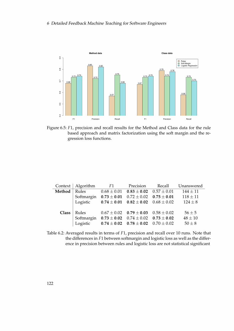
6 Detailed Feedback Machine Teaching for Software Engineers
F1 Precision Recall
RulesSoft MarginLogistic Regression
Class data
0.67
0.73 0.74
0.79
0.74
0.78
0.58
0.73
0.70
F1 Precision Recall
Method data
0.4
0.5
0.6
0.7
0.8
0.9
0.68
0.73 0.74
0.83
0.72
0.82
0.57
0.75
0.68
Figure 6.5: F1, precision and recall results for the Method and Class data for the rulebased approach and matrix factorization using the soft margin and the re-gression loss functions.
Context Algorithm F1 Precision Recall UnansweredMethod Rules 0.68± 0.01 0.83± 0.02 0.57± 0.01 144± 11
Softmargin 0.73± 0.01 0.72± 0.02 0.75± 0.01 118± 11Logistic 0.74± 0.01 0.82± 0.02 0.68± 0.02 124± 8
Class Rules 0.67± 0.02 0.79± 0.03 0.58± 0.02 56± 5Softmargin 0.73± 0.02 0.74± 0.02 0.73± 0.02 48± 10Logistic 0.74± 0.02 0.78± 0.02 0.70± 0.02 50± 8
Table 6.2: Averaged results in terms of F1, precision and recall over 10 runs. Note thatthe differences in F1 between softmargin and logistic loss as well as the differ-ence in precision between rules and logistic loss are not statistical significant
122

6.5 Evaluation Results and Discussion
We observe that the matrix factorization algorithm with a logistic regression loss per-forms best in terms of the F1 score, closely matched by the soft margin loss. Matrix fac-torization overall performs significantly better than the rule based approach in terms ofthe F1 score. However, both loss functions show very different performance character-istics: For the logistic regression loss, recall and precision differ significantly while theperformance of the soft margin loss function is more balanced.
Influence of the weight
Note that precision and recall are very sensitive to the value of g+, the positive weight.Thus, a desired balance between the two measures can be easily achieved by tweakingthis value.
Figure 6.6 depicts the relation between the performance measures and the weight pa-rameter for the matrix factorization system with a soft margin loss. As to be expected,the value of precision decreases as the positive weight increases. The recall behaves inan inverse manner and increases as the weight goes up. The optimal value of the F1 isreached for the weight value 10 (2.3 in the log plot). The weight parameter thus pro-vides a convenient way of adjusting the performance of the system to the requirementsof the particular situation.
Influence of the number of factors:
Another interesting parameter to study is the number of factors and its impact on sys-tem performance. The run-time performance of the system is almost only determinedby its value.
Figure 6.7 depicts the values of F1, precision and recall for different numbers of fac-tors for the soft margin loss function. We observe that for about 30 factors the systemreaches an almost optimal performance while further increases do not affect the perfor-mance in terms of the F1 score in a significant way.
Runtime performance
Training the initial model takes about 7 minutes for the class context data and 25 min-utes for the method context data using the logistic loss function. Based on this model,the system can predict calls in a few milliseconds in the current scenario. This is fastenough to implement the algorithm within an interactive environment.
The main memory needed is the one for C, as R can be discarded after initial training.C for 45 factors needs 1557 ∗ 45 ∗ 8 Bytes = 547 kBytes of memory. This also is easilyavailable on a developer workstation.
123

6 Detailed Feedback Machine Teaching for Software Engineers
0 2 4 6 8
0.0
0.2
0.4
0.6
0.8
1.0
log(weight)
F1PrecisionRecall
Figure 6.6: F1, precision and recall for the matrix factorization system with a soft mar-gin loss for different value of the weight parameter (on a natural log scale)
124

6.5 Evaluation Results and Discussion
0 50 100 150 200 250
0.2
0.3
0.4
0.5
0.6
0.7
0.8
0.9
Number of factors
F1PrecisionRecall
Figure 6.7: Results for F1, precision and recall obtained with the matrix factorizationsystem with a soft margin loss and different values for the number of factorsparameter
125

6 Detailed Feedback Machine Teaching for Software Engineers
6.6 Conclusion
We presented an application of the Detailed Machine Teaching approach in this chapter.As before, the focus was on the question whether a machine learning model, namelythe matrix factorization approach described in Chapter 4 can be applied to the task ofgenerating detailed feedback for learners.
We chose the software engineering domain for this evaluation, as source code is natu-rally digital and well structured. Both of which render source code analysis suitable forthis evaluation. In addition to this easy availability and interpret-ability of the artifacts,the knowledge needed to create them is usually not externalized. These observationsmake software engineering a suitable target for an evaluation of the Detailed FeedbackMachine Teaching approach.
The results, which were obtained based upon a simulated programmer, indicate thatthe machine learning model is indeed capable of capturing important knowledge fromthe provided expert code. This is especially noteworthy, as we did not perform anyadaptations of the model and algorithm as introduced in Chapter 4: The main designdecision was to decide for the structural elements to operate on and for a loss function.Both decisions are inevitable and do not form a special case for the application in thischapter.
Thus, the argument from Section 2.5 on page 47 proofed itself to be true in this ex-ample: Even if one could design a machine learning model for each kind of artifact, itis not always necessary for sufficient performance. Future work should investigate thesuitability of the algorithm presented in Chapter 4 to further substantiate that claim.
The results also show empirically that the algorithm meets the requirements set outfor a recommender system to be used in Machine Teaching in Section 2.5 on page 49 inthis application domain, namely:
R1: Accurate solutions for partial artifacts: As we have described, the system is capa-ble of predicting well given 50 % of structural elements, in this case of the calls ina context.
R2: Interactive Performance: Prediction generally took only a few milliseconds. Obvi-ously, this is fast enough for interactive use of the system, where a response timesof up to 0.1 seconds are generally considered to be unnoticeable (see e. g. [Mil68]and [NL06], Chapter 5).
This performance, coupled with the low memory footprint, also facilitates furtherapplication of the approach to the multi-framework case where the number ofpotential callees rises significantly.
R3: Recommendation Coherence: This again follows from the evaluation results: Thesystem achieved high precision scores in the order of 0.75 which indicate that itwas indeed capable of providing coherent suggestions to the user. This is espe-cially notable as the system showed a far higher recall than the baseline system.
126

6.6 Conclusion
R4: Easy Adaptation to Multiple Types of Prediction: Through choosing the weightedvariants of the logistic and hinge loss functions, we adapted the system to the typeor prediction necessary in this case.
Even though specialized models may outperform the application of the rather gen-eral matrix factorization framework done here, it is thus safe to conclude that the ma-chine learning aspect of Detailed Feedback Machine Teaching can be provided by ma-trix factorization models, especially by the one introduced in Chapter 4 of this thesis.The predictions generated are accurate and quickly available, even in the case wherechanged artifacts occur frequently.
127


7 Conclusions
129

7 Conclusions
7.1 Summary
Problem Statement By its very design, current Technology Enhanced learning sys-tems cannot convey knowledge that is not standardized, structured and most of all ex-ternalized. However, important knowledge such as intuition, experience or more gen-erally speaking implicit knowledge does not meet these requirements. Additionally,the structured externalization of knowledge in the form of electronic learning materialis often impossible for economic reasons, as its creation is costly.
In traditional education, the apprenticeship with its master-student relationship isused to convey this knowledge. In this setting, the master explains to, discusses withand corrects the learner in a situation centered around the learned activity. This ap-proach is very effective. Yet, it by design requires the availability of a master in the fieldto the learner.
Approach MACHINE TEACHING is proposed in this thesis to overcome these limita-tions: We notice that knowledge, even if not standardized, structured and externalized,can still be observed through its application. We refer to this observable knowledgeas PRACTICED KNOWLEDGE. Machine Teaching is build upon this notion: MachineLearning techniques are used to extract machine models of Practiced Knowledge fromobservational data. The models thus capture traces of the Practiced Knowledge thatwent into the artifacts and processes, be it implicit or explicit. These models are thenapplied in the learner’s context for his support.
It is important to note that the people creating the artifacts or following the processesneed not to be aware of their role in the system: They are not teachers, they are prac-titioners. Therefore, Machine Teaching focuses on the practice, not the ideal, just as theapprenticeship.
While both processes and artifacts can be the anchor in a Machine Teaching scenario,the automatic detection of processes still is an open field of research. As this is a pre-condition to a successful implementation of a Machine Teaching system, the thesis putsa focus on artifacts.
Levels of Feedback
We identified two important sub-classes of Machine Teaching: General and DetailedFeedback Machine Teaching.
General Feedback Machine Teaching General feedback in a way is like the gradesgiven at school: Given an artifact, the Machine Teaching system determines its qual-ity. This is a straight-forward application of techniques from the field of supervisedmachine learning and the main effort in building a specific Machine Teaching Systemlies in deriving appropriate feature extraction procedures. Thus, General Feedback Ma-chine Teaching is readily applicable to a wide range of scenarios where the featureengineering task is either straight-forward or has been studied to great extend. This in-cludes tasks related to text, images and of course artifacts which exhibit feature-vector
130

7.1 Summary
structure themselves. The application presented in this thesis, learning to write for aspecific community, shows that the approach is viable and that the predicted quality ofthe artifact can in fact be very close to the one perceived by the community.
Detailed Feedback Detailed Feedback Machine Teaching aims at providing feedbackregarding the attributes of the artifact to the learner. To do so, the machine learningmodel needs to have a notion of these artifact and their relations. This, in principle,provokes the creation of a specific machine learning model for each detailed feedbackapplication of Machine Teaching. However, it has been shown in this thesis that De-tailed Feedback Machine Teaching often exhibits a striking similarity to the task of arecommender system. Where the latter suggests items to customers, the former “sug-gests” attributes to artifacts. Despite this obvious similarity, Machine Teaching posesadditional requirements onto the underlying algorithm not usually occurring in Rec-ommender Systems. These include a greater variety in the attributes of artifacts, thefrequent prediction upon yet unseen artifacts and the real-time nature of a MachineTeaching system. Last but not least, Detailed Feedback Machine Teaching imposes con-sistency requirements for one artifact as a whole, while a Recommender System is usu-ally focused on predicting the rating a user would associate with a single item.
Matrix Factorization Model and Method This thesis presented a novel model and al-gorithm based on factor models that substantially generalizes the state-of-the-art inthis field to address these requirements uniquely found in Machine Teaching. The al-gorithm is a valuable contribution to the field of Recommender Systems in its own rightas it is the first to be able to predict rankings as opposed to ratings. Additionally, it formsa hybrid Recommender System that can use known features of the user (artifacts) anditems (structural elements) in addition to the collaborative effect present in such data.The base algorithm as well as the extensions thereof proposed in this thesis have shownfavorable performance on standard Recommender Systems evaluation data sets avail-able. It is important to note that the algorithm excels especially in what is called thenew-user problem in Recommender Systems: Given a new, yet unseen user with somerated items and a trained model based on other users, the goal is to predict well for thisnew user. While this situation is the exception in Recommender Systems, it is the normin Machine Teaching: every time the learner presents the system with an artifact, thatartifact constitutes a “new user”. Thus, excellent predictive performance on this task iscrucial for Machine Teaching.
Machine Teaching for Software Engineering The domain of learning to program wellwithin a software framework is modeled as a task for Detailed Feedback MachineTeaching by forming a caller-callee matrix of representative code. This matrix storesevery call to the software framework from the code analyzed, where each row repre-sents one method or class of the analyzed code and each column represents a possiblycallable method of the framework. The goal of a Machine Teaching system when con-fronted with a partial row is to predict missing calls. As we have shown in the empirical
131

7 Conclusions
evaluation, the model is capable of capturing the structure in this matrix and can there-fore compute meaningful feedback for the learning programmer.
This application exemplifies the expressive power of the factor model presented inthis thesis, as the model was applied to the problem in a straight-forward manner. Soeven while purpose-built models are likely to perform even better, the factor modelcan serve as the underlying model for a wide range of Machine Teaching applications.It therefore provides Detailed Feedback Machine Teaching with a foundation just assupervised machine learning forms the base of General Feedback Machine Teaching.
7.2 Future Work
In this thesis, it was successfully demonstrated that machine learning models can mineartifacts to compute feedback for learners. Future work can build upon this result toaddress additional challenges of a Machine Teaching System.
Open Questions in Machine Teaching
The User Interface: The feedback computed following the methodology introducedin this thesis needs to be presented to the learner in a useful way. For the softwaredevelopment scenario, we hypothesized that the presentation could be done sim-ilarly to that of compiler warning and errors as depicted in Figure 6.1 on page 113.
For many other domains, this question of the user interface is essentially open.Further studies should reveal if and how much the feedback user interface forMachine Teaching differs from traditional systems where the underlying modelis designed as opposed to machine learned.
User Studies: Given a user interface, the next step would be a user study. MachineTeaching, especially when used without the distinction between Learners and Ex-perts, may give rise to new or adapted use patterns. One question to study wouldbe whether experts use a Machine Teaching system differently from novices andif both use cases lead to learning.
Feature Engineering for Detailed Feedback: As introduced above, the matrix factor-ization algorithm can make use of row and column features if they are available.While the software engineering system obtained good results without them, fur-ther improvements are possible. In the software engineering domain, these fea-tures can be extracted using static code analysis.
Matrix Factorization Improvements
Factor models are an active field of research and the model presented in Chapter 4 pro-vides a solid framework to integrate current results from the field as well as upcomingresearch directions such as:
132

7.2 Future Work
Use of Hierarchies: In many instances, the rows or columns of the input matrix forma hierarchy. In Recommender Systems, these hierarchies can be the result of e. g.movie sequels, editions or, for the users, the hierarchy induced by the addressesof the users. Hierarchies almost naturally occur in the software engineering ap-plication of the Machine Teaching approach:
• Statements are part of methods; methods are part of classes and they them-selves are organized into packages, name spaces or modules.
• Programmers belong to a team which belongs to a department which is partof a larger institution. The coding style and conventions can be assumed tobe increasingly detailed from the top to the base of this hierarchy.
Using these and other hierarchies can not only increase the predictive perfor-mance of a factor model, it can also allow it to fail in a more grateful mannerby suggesting at least a movie from the right genre if failing to suggest the mostlikely movie. In Machine Teaching, a system could e. g. fail to suggest the rightcall, yet be able to predict that a call on a certain object is missing.
There are currently no systems that can make use of this information in the factormodels realm. The topic is, however, in the focus of a track of research in super-vised machine learning under the term “feature hierarchies“. Further researchcould investigate the transfer, adaptation and augmentation of these results tofactor models.
Fixed Memory Factor Models: Many Recommender Systems are faced with millionsof items and users. Another large-scale problem, which Collaborative Filter-ing has been recently applied to, is advertisement placement, where one essen-tially deals with as many “users” as the number of websites as described e. g.in [ABC+07]. Storing the matrices R and C in main memory is infeasible for thesescenarios.
There is a growing interest in what is called hash models in machine learning thatcompress the model by depending on the collisions of a hash function. Follow-ing [WDA+09], this idea can be transferred to factor models by defining a hashfunction on the rows and columns. Depending on the application, the collisions ofthis hash function may either be entirely random, or based upon features knownabout the rows and columns. One can then scale the memory requirement byfixing the hash function to output only a certain number of results to escape thelinear scaling of factor models.
Note that this is not the same application of hash functions as in feature hashingas used e. g. by Vowpal Wabbit as described in [LLS07]. In these on-line learningapproaches, the number of features in the input domain is reduced to a fixed sizein order to gain computational efficiency. In our terms, that would be similar toreducing the number of factors d by means of hashing. In our approach, this isunnecessary as d is a parameter in our case, while it is fixed in normal classifica-tion or regression problems where it represents the number of features. In these
133

7 Conclusions
types of problems that number can be huge, e. g. when dealing with text wherethe presence of every word is typically treated as a feature.
Online Learning: As introduced above, the factor model is trained in offline mode:Given the data matrix Y, the system finds the model matrices C and R. In manycases, an online training is more appropriate where the model is built from aconstant stream of new entries in Y. As we have seen in Section 4.5.3 on page 96,the model can be adapted to new rows easily. The same idea cannot be extendedto new columns under the assumptions of Chapter 4, as we explicitly supportper-row loss functions.
If one assumes element-wise losses, it is well known that Factor Models can bebuilt in an online fashion using algorithms such as the Stochastic Gradient De-scent. Future research is necessary to investigate possible approximations or for-mulations of the model with per-row losses that facilitate online updates.
Factor Models with Context Aware Biases: Recently, a factor model was proposed forthe field of Recommender Systems that explicitly models the temporal effect ofa Recommender System by essentially making the row and column biases timedependent in [Kor09]. The reasoning for Recommender Systems is that the pref-erences of users change over time and that the overall preference changes overtime, too, e. g. because of a successful product placement in a national TV show.
As hinted above, this proposal can be integrated into the framework of this thesisby having different column and row biases for different times.
In a broader view, this recent development hints at context-aware factor mod-els. In the example above, time served as the context and as such linked the rowand column biases. It would be interesting to extend this concept to features ofthe matrix elements. In Recommender Systems, that would be features of a rat-ing and the premier example of such a feature is the time at which the rating isgiven or asked to be predicted. Other useful sources of context for e. g. the movieRecommender System would be the intended audience of the movie as the rec-ommendations in e. g. a family should differ depending on whether a movie issought for just the parents or the whole family.
In Machine Teaching, such a system opens additional avenues for tailoring thesuggestions to the user by using the user features as context. Informally, the sys-tem would no longer form predictions like “In other instances, people also didA.” to more personalized ones like “In other instances, people like you also didA.” This raises subsequent questions in the application domain such as how todefine a similarity measure on learners and under which circumstances a person-alization helps or hinders the learning.
Sequence Prediction: In many Machine Teaching scenarios, ordered entries in the rowsoccur naturally, e. g. in the software engineering domain where a file needs to beclosed after it has been opened. One naive way of supporting this is to encode inYi, j the position at which call j was made in context i. Then, the ordinal regression
134

7.2 Future Work
loss function can be used to build a model that can predict these orderings. How-ever, this approach is rather ad-hoc and is rather impractical for the followingreasons:
• There is no principled way to deal with repetitions which frequently occurin real data.
• Such a model can only predict the ordering of the calls, but not the presenceof them. This could be solved by yet another ad-hoc fix by building a secondmodel e. g. based on the logistic regression loss.
Thus, a more principled solution to this task is needed. Markov Models probablycan serve as an inspiration in finding one. A solution would likely be based onthe following idea: The prediction rule of the model needs to be extended suchthat a prediction Fi, j depends not only on Ri and C j but also a number of those Ckwhich occurred prior to Yi, j in Yi,∗. It is plausible that a model around this notioncan be build by extending the one presented here.
As we have shown, Machine Teaching opens a wide range of research questions in itsapplication but also poses new challenges to the underlying machine learning models.
135


7.2 Future Work
Wissenschaftlicher Werdegang des Autors
2007 und 2008: Forschungsaufenthalte in Australien. Mitarbeit in der Gruppe ,,Sta-tistical Machine Learning” von NICTA, Canberra unter Leitung von Prof. AlexSmola.
2006, 2007 und 2008: Teilnahme an den Machine Learning Summer Schools in Can-berra (Australien), Tubingen und Kioloa(Australien).
2005: Abschluss des Diplomstudiengangs Wirtschaftsinformatik an der TU Darmstadtmit Auszeichnung.
2005: Diplomarbeit ,,Genetic Mineplanning – a genetic algorithm approach to mineplanning” bei Prof. Karsten Weihe.
2004: Studienaufenthalt am Centre for Complex Dynamic Systems and Control at TheUniversity Of Newcastle (Australien) zur Erstellung der Studienarbeit ,,Optimiz-ing Flexibility – a new approach to cope with uncertainty in the mining industryand beyond”. Betreuer: Prof. Karsten Weihe und Prof. Wolfgang Domschke.
2002: Studienarbeit ,,Entwicklung eines Mechatronik-Frameworks fur das Projekt Laufer”bei Prof. Sorin Huss, TUD.
1999: Aufnahme des Diplomstudiengangs Wirtschaftsinformatik an der TU Darmstadt
1998: Abitur an der Furst-Johann-Ludwig Schule in Hadamar in den LeistungskursenMathematik und Physik.
137


Bibliography
[AB06] Yigal Attali and Jill Burstein. Automated essay scoring with e-rater v.2. TheJournal of Technology, Learning, and Assessment, 4(3), February 2006.
[ABC+07] Deepak Agarwal, Andrei Z. Broder, Deepayan Chakrabarti, Dejan Diklic,Vanja Josifovski, and Mayssam Sayyadian. Estimating rates of rare eventsat multiple resolutions. In Proceedings of the 13th ACM SIGKDD InternationalConference on Knowledge Discovery and Data Mining. ACM Press, 2007.
[ABEV06] Jacob Abernethy, Francis Bach, Theodoros Evgeniou, and Jean-Philippe Vert. Low-rank matrix factorization with attributes. CoRR,abs/cs/0611124, 2006.
[AC09] Deepak Agarwal and Bee-Chung Chen. Regression-based latent factormodels. In KDD ’09: Proceedings of the 15th ACM SIGKDD internationalconference on Knowledge discovery and data mining, pages 19–28, New York,NY, USA, 2009. ACM.
[AG01] John Robert Anderson and Kevin A. Gluck. What role do cognitive architec-tures play in intelligent tutoring systems?, pages 227–262. Erlbaum, 2001.
[AG09] IM-C AG. Lecturnity. http://www.lecturnity.com, August 2009.
[AT05] Gediminas Adomavicius and Alexander Tuzhilin. Toward the next genera-tion of recommender systems: A survey of the state-of-the-art and possibleextensions. IEEE Transactions on Knowledge and Data Engineering, 17(6):734–749, June 2005.
[BH04] Justin Basilico and Thomas Hofmann. Unifying collaborative and content-based filtering. In Proceedings of the International Conference on Machine Lear-ing, pages 65–72, New York, NY, 2004. ACM Press.
[Bis06] Christopher M. Bishop. Pattern Recognition and Machine Learning. Informa-tion Science and Statistics. Springer, 2006.
[BJ94] Kent Beck and Ralph E. Johnson. Patterns generate architectures. In Pro-ceedings of the European Conference on Object-Oriented Programming, pages139–149. Springer, 1994.
[BKM00] Greg Butler, Rudolf K. Keller, and Hafedh Mili. A framework for frame-work documentation. ACM Computing Surveys, 32(1):15–21, 2000.
139

Bibliography
[BKV07] Robert Bell, Yehuda Koren, and Chris Volinsky. The bellkor so-lution to the neflix prize. Technical report, AT&T Labs, 2007.http://www.netflixprize.com/assets/ProgressPrize2007 KorBell.pdf.
[Bla09] Blackboard. Blackboard. http://www.blackboard.com, August 2009.
[BMM09] Marcel Bruch, Martin Monperrus, and Mira Mezini. Learning from exam-ples to improve code completion systems. In Proceedings of 17th ACM SIG-SOFT Symposium on the Foundations of Software Engineering, August 2009.
[BMRC09] Oliver Brdiczka, Jerome Maisonnasse, Patrick Reignier, and James L.Crowley. Detecting small group activities from multimodal observations.Applied Intelligence, 30(1):47–57, 2009.
[Bot04] Leon Bottou. Stochastic learning. In Olivier Bousquet and Ulrike vonLuxburg, editors, Advanced Lectures on Machine Learning, Lecture Notes inArtificial Intelligence, LNAI 3176, pages 146–168. Springer Verlag, Berlin,2004.
[BSM06] Marcel Bruch, Thorsten Schafer, and Mira Mezini. FrUiT: IDE supportfor framework understanding. In Proceedings of the OOPSLA Workshop onEclipse Technology Exchange, pages 55–59. ACM Press, 2006.
[CB04] Martin Chodorow and Jill Burstein. Beyond essay length: Evaluating e-raters performance on toefl essays. Technical report, ETS, 2004.
[CG05] Wei Chu and Zoubin Ghahramani. Gaussian processes for ordinal regres-sion. Journal of Machine Learning Research, 6:1019–1041, 2005.
[Com09a] The Moodle Community. Moodle. http://moodle.org, August 2009.
[Com09b] The Sakai Community. Sakai. http://sakaiproject.org, August2009.
[CSS00] Michael Collins, Robert E. Schapire, and Yoram Singer. Logistic regres-sion, AdaBoost and Bregman distances. In Proc. 13th Annu. Conference onComput. Learning Theory, pages 158–169. Morgan Kaufmann, San Francisco,2000.
[DBSS06] Paul De Bra, David Smits, and Natalia Stash. The design of aha! In HY-PERTEXT ’06: Proceedings of the seventeenth conference on Hypertext and hy-permedia, pages 133–134, New York, NY, USA, 2006. ACM.
[DSSS05] Ofer Dekel, Shai Shalev-Shwartz, and Yoram Singer. Smooth ε-insensitiveregression by loss symmetrization. Journal of Machine Learning Research,6:711–741, 2005.
140

Bibliography
[EN08] Charles Elkan and Keith Noto. Learning classifiers from only positive andunlabeled data. In Proceedings of the ACM Conference on Knowledge Discoveryand Data Mining (KDD). ACM, 2008.
[FN87] W.B. Frakes and B.A. Nejmeh. Software reuse through information re-trieval. SIGIR Forum, 21(1-2):30–36, 1987.
[Fou09] The Eclipse Foundation. The eclipse ide. http://www.eclipse.org,August 2009.
[GM96] Dipayan Gangopadhyay and Subrata Mitra. Design by framework com-pletion. Automated Software Engineering, 3(3/4):219–237, 1996.
[GMM+07] Iryna Gurevych, Max Muhlhauser, Christof Muller, Jurgen Steimle,Markus Weimer, and Torsten Zesch. Darmstadt Knowledge ProcessingRepository Based on UIMA. In Proceedings of the First Workshop on Unstruc-tured Information Management Architecture at Biannual Conference of the So-ciety for Computational Linguistics and Language Technology, Tubingen, Ger-many, April 2007.
[goo] Google code search. http://www.google.com/codesearch.
[Hen91] Scott Henninger. Retrieving software objects in an example-based pro-gramming environment. In Proceedings of the SIGIR International Conferenceon Research and Development in Information Retrieval, pages 251–260. ACMPress, 1991.
[HGO00] Ralf Herbrich, Thore Graepel, and Klaus Obermayer. Large margin rankboundaries for ordinal regression. In Alexander J. Smola, P. L. Bartlett,B. Scholkopf, and D. Schuurmans, editors, Advances in Large Margin Classi-fiers, pages 115–132, Cambridge, MA, 2000. MIT Press.
[HHG90] Richard Helm, Ian M. Holland, and Dipayan Gangopadhyay. Contracts:Specifying behavioral compositions in object-oriented systems. In Proceed-ings of the Conference on Object-Oriented Programming, Systems, Languages,and Applications and the European Conference on Object-Oriented Programming,pages 169–180. ACM Press, 1990.
[HKV08] Yifan Hu, Yehuda Koren, and Chris Volinsky. Collaborative filtering forimplicit feedback datasets. In Proceedings of the IEEE International Conferenceon Data Mining (ICDM), 2008.
[HM05] Reid Holmes and Gail C. Murphy. Using structural context to recommendsource code examples. In Proceedings of the International Conference on Soft-ware Engineering, pages 117–125. ACM Press, 2005.
[Hul94] David Hull. Improving text retrieval for the routing problem using latentsemantic indexing. In SIGIR ’94: Proceedings of the 17th annual international
141

Bibliography
ACM SIGIR conference on Research and development in information retrieval,pages 282–291, New York, NY, USA, 1994. Springer-Verlag New York, Inc.
[Joa06] Thorsten Joachims. Training linear SVMs in linear time. In Proceedings ofthe ACM Conference on Knowledge Discovery and Data Mining (KDD). ACM,2006.
[Joh92] Ralph E. Johnson. Documenting frameworks using patterns. In Proceedingsof the Conference on Object-oriented Programming, Systems, Languages, and Ap-plications, pages 63–72. ACM Press, 1992.
[Kor09] Yehuda Koren. Collaborative filtering with temporal dynamics. In Proceed-ings of the 15th ACM SIGKDD Conference on Knowledge Discovery and DataMining (KDD), 2009.
[KPCP06] Soo-Min Kim, Patrick Pantel, Tim Chklovski, and Marco Penneacchiotti.Automatically assessing review helpfulness. In Proceedings of the Conferenceon Empirical Methods in Natural Language Processing (EMNLP), pages 423 –430, Sydney, Australia, July 2006.
[KSF+06] Jihie Kim, Erin Shaw, Donghui Feng, Carole Beal, and Eduard Hovy. Mod-eling and assessing student activities in on-line discussions. In Proceedingsof the Workshop on Educational Data Mining at the conference of the AmericanAssociation of Artificial Intelligence (AAAI-06), Boston, MA, 2006.
[KSH09] Alexandros Karatzoglou, Alexander J. Smola, and Kurt Hornik. Cran pack-age kernlab 0.9-8 - kernel-based machine learning, 2009.
[KSHZ04] Alexandros Karatzoglou, Alexander J. Smola, Kurt Hornik, and AchimZeileis. kernlab – an S4 package for kernel methods in R. Journal of Sta-tistical Software, 11(9):1–20, 2004.
[KW10] Alexandros Karatzoglou and Markus Weimer. Collaborative PreferenceLearning, chapter (to appear). Springer Verlag, 2010.
[Lea09] Advanced Distributed Learning. Scorm. http://www.adlnet.gov/Technologies/scorm/, August 2009.
[LL03] Wee Sun Lee and Bing Liu. Learning with positive and unlabeled examplesusing weighted logistic regression. In Proceedings of the 20th InternationalConference on Machine Learning (ICML 2003). AAAI Press, 2003.
[LLS07] John Langford, Lihong Li, and Alex Strehl. Vowpal wabbit online learningproject. Technical report, Yahoo! Research, 2007. http://hunch.net/?p=309.
[LMA87] Matthew W. Lewis, Robert Milson, and John R. Anderson. The teacher’sapprentice: Designing an intelligent authoring system for high schoolmathematics. pages 269–301, 1987.
142

Bibliography
[LR04] Cliff Lampe and Paul Resnick. Slash(dot) and burn: Distributed modera-tion in a large online conversation space. In Proceedings of ACM CHI 2004Conference on Human Factors in Computing Systems, Vienna Austria, pages543–550, 2004.
[LZ05a] Zhenmin Li and Yuanyuan Zhou. PR-Miner: Automatically extracting im-plicit programming rules and detecting violations in large software code.In Proceedings of the European Software Engineering Conference, pages 306–315. ACM Press, 2005.
[LZ05b] Benjamin Livshits and Thomas Zimmermann. Dynamine: finding com-mon error patterns by mining software revision histories. In Proceedings ofthe ACM SIGSOFT International Symposium on Foundations of Software Engi-neering, pages 296–305. ACM Press, 2005.
[MGNR06] Edward Meeds, Zoubin Ghahramani, Radford Neal, and Sam Roweis.Modeling dyadic data with binary latent factors. In Advances in NeuralInformation Processing Systems 20, Cambridge, MA, 2006. MIT Press.
[Mic00] Amir Michail. Data mining library reuse patterns using generalized asso-ciation rules. In Proceedings of the International Conference on Software Engi-neering, pages 167–176. ACM Press, 2000.
[Mil68] R. B. Miller. Response time in man-computer conversational transactions.In Proceedings of the AFIPS Fall Joint Computer Conference, volume 33, 1968.
[MSM94] Mitchell P. Marcus, Beatrice Santorini, and Mary Ann Marcinkiewicz.Building a Large Annotated Corpus of English: The Penn Treebank. Com-putational Linguistics, 19(2):313–330, 1994.
[MWK+06] Ingo Mierswa, Michael Wurst, Ralf Klinkenberg, Martin Scholz, and TimmEuler. YALE: Rapid prototyping for complex data mining tasks. In KDD’06: Proceedings of the 12th ACM SIGKDD international conference on Knowl-edge discovery and data mining, pages 935–940, New York, NY, USA, 2006.ACM Press.
[MXBK05] David Mandelin, Lin Xu, Rastislav Bodık, and Doug Kimelman. Jungloidmining: helping to navigate the api jungle. In Proceedings of the ACMSIGPLAN Conference on Programming Language Design and Implementation,pages 48–61. ACM Press, 2005.
[NL06] Jakob Nielsen and Hoa Loranger. Prioritizing web usability. New Riders,Berkeley, California, 2006.
[NW99] J. Nocedal and S. J. Wright. Numerical Optimization. Springer Series inOperations Research. Springer, 1999.
143

Bibliography
[PS09] Rong Pan and Martin Scholz. Mind the gaps: Weighting the unknown inlarge-scale one-class collaborative filtering. In Proceedings of the 15th ACMSIGKDD Conference on Knowledge Discovery and Data Mining (KDD), 2009.
[QABC09] LLC Quality Alliance Business Consultants. Power trainer. http://www.powertrainer.net, August 2009.
[RS05] Jasson D. M. Rennie and Nathan Srebro. Fast maximum margin matrixfactorization for collaborative prediction. In ICML ’05: Proceedings of the22nd international conference on Machine learning, pages 713–719, New York,NY, USA, 2005. ACM.
[Sch95] Helmut Schmid. Probabilistic Part-of-Speech Tagging Using DecisionTrees. In International Conference on New Methods in Language Processing,Manchester, UK, 1995.
[SEHM06] Thorsten Schafer, Michael Eichberg, Michael Haupt, and Mira Mezini. TheSEXTANT software exploration tool. IEEE Transactions on Software Engi-neering, 32(9):753–768, 2006.
[SG08] Ajit P. Singh and Geoff J. Gordon. A unified view of matrix factorizationmodels. In Machine Learning and Knowledge Discovery in Databases, EuropeanConference (ECML/PKDD), 2008. ECML/PKDD-2008.
[SJ03] N. Srebro and T. Jaakkola. Weighted low-rank approximations. In Proceed-ings of the 20th International Conference on Machine Learning (ICML 2003),pages 720 – 727. AAAI Press, 2003.
[SLB00] Forrest Shull, Filippo Lanubile, and Victor R. Basili. Investigating readingtechniques for object-oriented framework learning. IEEE Transactions onSoftware Engineering, 26(11):1101–1118, 2000.
[SM08] Ruslan Salakhutdinov and Andriy Mnih. Probabilistic matrix factorization.In J.C. Platt, D. Koller, Y. Singer, and S. Roweis, editors, Advances in NeuralInformation Processing Systems 20, volume 20, pages 1257–1264, Cambridge,MA, 2008. MIT Press.
[SRJ05] Nathan Srebro, Jason D. M. Rennie, and Tommi S. Jaakkola. Maximum-margin matrix factorization. In Lawrence K. Saul, Yair Weiss, and LeonBottou, editors, Advances in Neural Information Processing Systems 17, pages1329–1336. MIT Press, Cambridge, MA, 2005.
[SS02] Bernhard Scholkopf and Alexander J. Smola. Learning with Kernels. MITPress, Cambridge, MA, 2002.
[SS05] Nathan Srebro and Adi Shraibman. Rank, trace-norm and max-norm. InP. Auer and R. Meir, editors, Proceedings of the Annual Conference on Compu-tational Learning Theory, number 3559 in Lecture Notes in Artificial Intelli-gence, pages 545–560. Springer-Verlag, June 2005.
144

Bibliography
[SVL08] Alexander J. Smola, S.V.N. Vishwanathan, and Quoc Viet Le. Bundle meth-ods for machine learning. In Advances in Neural Information Processing Sys-tems 20, Cambridge, MA, 2008. MIT Press.
[TGK04] B. Taskar, C. Guestrin, and D. Koller. Max-margin Markov networks. InS. Thrun, L. Saul, and B. Scholkopf, editors, Advances in Neural InformationProcessing Systems 16, pages 25–32, Cambridge, MA, 2004. MIT Press.
[TJHA05] Ioannis Tsochantaridis, Thorsten Joachims, Thomas Hofmann, andYasemin Altun. Large margin methods for structured and interdependentoutput variables. Journal Of Machine Learning Research, 6:1453–1484, 2005.
[TPNT07] G. Takacs, I. Pilaszy, B. Nemeth, and D. Tikk. Major components of thegravity recommendation system. SIGKDD Explorations Newsletter, 9(2):80–83, 2007.
[Vap95] Vladimir Vapnik. The Nature of Statistical Learning Theory. Springer, NewYork, 1995.
[Vap98] Vladimir Vapnik. Statistical Learning Theory. John Wiley and Sons, NewYork, 1998.
[VGS97] Vladimir Vapnik, Steven E. Golowich, and Alexander J. Smola. Supportvector method for function approximation, regression estimation, and sig-nal processing. In M. C. Mozer, M. I. Jordan, and T. Petsche, editors,Advances in Neural Information Processing Systems 9, pages 281–287, Cam-bridge, MA, 1997. MIT Press.
[VNC03] Salvatore Valenti, Francesca Neri, and Alessandro Cucchiarelli. Anoverview of current research on automated essay grading. Journal of In-formation Technology Education, 2:319–329, 2003.
[Voo01] E. Voorhees. Overview of the TRECT 2001 question answering track. InTREC, 2001.
[WDA+09] Kilian Weinberger, Anirban Dasgupta, Josh Attenberg, John Langford, andAlexander J. Smola. Feature hashing for large scale multitask learning. InProceedings of International Conference on Machine Learning (ICML), 2009.
[WF05] Ian H. Witten and Eibe Frank. Data Mining: Practical machine learning toolsand techniques. Morgan Kaufmann, San Francisco, 2 edition, 2005.
[WG07] Markus Weimer and Iryna Gurevych. Predicting the perceived quality ofweb forum posts. In Proceedings of the Conference on Recent Advances in Nat-ural Language Processing (RANLP), pages 643–648, 2007.
[WGM07] Markus Weimer, Iryna Gurevych, and Max Muhlhauser. Automatically as-sessing the post quality in online discussions on software. In Proceedings of
145
Bibliography
the 45th Annual Meeting of the Association for Computational Linguistics Com-panion Volume Proceedings of the Demo and Poster Sessions, pages 125–128,Prague, Czech Republic, June 2007. Association for Computational Lin-guistics.
[WKB09] Markus Weimer, Alexandros Karatzoglou, and Marcel Bruch. Maximummargin code recommendation. In RecSys ’09: Proceedings of the 2009 ACMconference on Recommender systems (to appear), 2009.
[WKLS08] Markus Weimer, Alexandros Karatzoglou, Quoc Viet Le, and Alexander J.Smola. Cofi rank - maximum margin matrix factorization for collaborativeranking. In J.C. Platt, D. Koller, Y. Singer, and S. Roweis, editors, Advancesin Neural Information Processing Systems 20, pages 1593–1600. MIT Press,Cambridge, MA, 2008.
[WKS08a] Markus Weimer, Alexandros Karatzoglou, and Alexander J. Smola. Adap-tive collaborative filtering. In RecSys ’08: Proceedings of the 2008 ACM con-ference on Recommender systems, pages 275–282, New York, NY, USA, 2008.ACM.
[WKS08b] Markus Weimer, Alexandros Karatzoglou, and Alexander J. Smola. Im-proving maximum margin matrix factorization. In Walter Daelemans, BartGoethals, and Katharina Morik, editors, Machine Learning and KnowledgeDiscovery in Databases, volume 5211 of LNAI, pages 14–14. Springer, 2008.
[WKS08c] Markus Weimer, Alexandros Karatzoglou, and Alexander J. Smola.Improving maximum margin matrix factorization. Machine Learning,72(3):263–276, 2008.
[WZL07] Andrzej Wasylkowski, Andreas Zeller, and Christian Lindig. Detectingobject usage anomalies. In Proceedings of the ACM SIGSOFT InternationalSymposium on Foundations of Software Engineering, pages 35–44. ACM Press,2007.
[XP06] Tao Xie and Jian Pei. MAPO: mining api usages from open source reposi-tories. In Proceedings of the International Workshop on Mining Software Repos-itories, pages 54–57. ACM Press, 2006.
[YC07] Kai Yu and Wei Chu. Gaussian process models for link analysis and trans-fer learning. In Advances in Neural Information Processing Systems 20, Cam-bridge, MA, 2007. MIT Press.
[YFR00] Yunwen Ye, Gerhard Fischer, and Brent Reeves. Integrating active informa-tion delivery and reuse repository systems. In Proceedings of the ACM SIG-SOFT International Symposium on Foundations of Software Engineering, pages60–68. ACM Press, 2000.
146

Bibliography
[YVGS08] Jin Yu, S. V. N. Vishwanathan, Simon Gunter, and Nicol N. Schraudolph.A quasi-newton approach to non-smooth convex optimization. In ICML’08: Proceedings of the 25th international conference on Machine learning, pages1216–1223, New York, NY, USA, 2008. ACM.
[YYTK06] Shipeng Yu, Kai Yu, Volker Tresp, and Hans-Peter Kriegel. Collaborativeordinal regression. In ICML ’06: Proceedings of the 23rd international con-ference on Machine learning, pages 1089–1096, New York, NY, USA, 2006.ACM.
[ZDLZ07] Zhongyuan Zhang, C. Ding, Tao Li, and Xiangsun Zhang. Binary matrixfactorization with applications. In Data Mining, 2007. ICDM 2007. SeventhIEEE International Conference on, pages 391–400, 2007.
[ZWS09] Andreas Zinnen, Christian Wojek, and Bernt Schiele. Multi activity recog-nition based on bodymodel-derived primitives. In Proceedings of the 4th In-ternational Symposium on Location and Context Awareness (LoCA), May 2009.
147

Bibliography
148