macroeconomic forecasting with independent component - repec

Macroeconomic Forecasting with Independent ComponentAnalysis

Ruey Yau

Department of Economics

Fu-Jen Catholic University

Taipei 242, Taiwan

ABSTRACT

This paper considers a factor model in which independent component analysis (ICA) is

employed to construct common factors out of a large number of macroeconomic time se-

ries. The ICA has been regarded as a better method to separate unobserved sources that

are statistically independent to each other. Two algorithms are employed to compute the

independent factors. The first algorithm takes into account the kurtosis feature contained

in the sample. The second algorithm accommodates the time dependence structure in the

time series data. A straightforward forecasting model using the independent factors is then

compared with the forecasting models using the principal components in Stock and Watson

(2002). The results of this research can help us to gain more knowledge about the underlying

economic sources and their impacts on the aggregate variables. The empirical findings sug-

gest that the independent component method is a powerful method of macroeconomic data

compression. Whether the ICA method is superior over the principal component method in

forecasting the U.S. real output and inflation variables is however inconclusive.

JEL classification: C32; C53; E60

Keywords: forecast, dynamic factors, independent component analysis, principal componentanalysis

1

1 Introduction

In the last two decades, enormous effort and progress have been made on the development

of small-scale macroeconometric models. Both stationary univariate autoregressions and

vector autoregressions (VARs) are standard benchmarks used to evaluate economic policies

or forecasts. These models include only a small number of variables while economic theories

usually suggest large categories of variables, such as output, money, interest rates, wages,

stock prices, etc. The choice of a specific subset of variables then becomes a statistical

problem (known as variable-selection problem).

As opposed to small-scale models, large-scale models explicitly incorporate information

from a large number of macroeconomic variables, again suggested by economic theory, into

a formal statistical framework. The large-model approach is more appealing in real world

practice because practical forecasters and policymakers find it useful to extract information

from many more series than are typically included in a VAR model. One advantage of the

large-model approach over the small-model approach is argued by Leeper et al. (1996) that

there may be substantial forecasting improvement as the number of variables increases from,

say 18 to 50 or to 100. Therefore, a VAR model with variables arbitrarily chosen might

have large biases associated with it. Furthermore, Watson (2000) shows empirical evidence

in support of the large model approach that there are many non-zero regression coefficients

in such models.1

One particular class of the large-scale model is known as factor models. Classical factor

models were initiated by Sargent and Sims (1977) and Geweke (1977) and had been consid-

ered in Singleton (1980), Engle and Watson (1981), Chamberlain and Rothschild (1983), and

Quah and Sargent (1983). More recent studies of this approach include Forni and Reichlin

(1996, 1998), Forni et al. (2000), and Stock and Watson (1998, 2002).

The intuition behind macroeconomic factor models is that the comovement in economic

time series is arising largely from a relatively few key economic factors, such as productivity,

monetary policy, oil shock, and so forth. In the literature, various methods have been

proposed to construct these common economic driving forces. Among them, the simplest

1A detailed discussion on the relative merits of the small and large model approaches can be found inWatson (2000).

2

method of constructing latent factors is the principal component analysis (PCA) introduced

by Stock and Watson (2002).2

Although economists have accumulated a vast amount of experiences and knowledge in

the theories of estimation, inferences and identification in a stationary VAR framework, there

are practical and theoretical questions applied to the large models need to be answered. In

particular, the problem of efficient estimation in large models remains an open question.

Naturally, the construction of the common economic factors would be crucial in determining

the forecasting performance of a factor model. While Stock and Watson’s method is readily

applied, their results also show that model selection procedures can be improved.

As an alternative to PCA, independent component analysis (ICA) is proposed in this

study to obtain economic factors. The reasons to advocate ICA are twofold. First, many

macroeconomic time series have fat tails in distribution and thus are non-Gaussian dis-

tributed. According to the central limit theorem, this implies that the latent economic

forces are farther away from being Gaussian distributed than the observed economic series.

While the ICA could construct factors that are non-Gaussian distributed, the PCA would

totally omit this possibility. Second, assumptions, such as orthogonality and stationarity,

are often made to identify latent factors. However, a researcher might be more interested in

factors that are statistically independent of each other. While the PCA is designed to sep-

arate factors that are uncorrelated, the ICA is able to separate factors that are statistically

independent.

We experimented with two different ICA algorithms in this paper. The basic ICA algo-

rithm is known as FastICA. The results suggest that the basic ICA is a powerful technique

of economic data compression; however its advantage over the PCA in forecasting the real

output and inflation of the United States is limited. One important issue had not been con-

sidered in the FastICA algorithm. The FastICA algorithm is ideally applied to data that have

no particular order. It means that one could shuffle the sample in anyway and this would

not affect the estimation of independent components (ICs). Nevertheless, macroeconomic

time series data contain much more time structure that should not be ignored. It implies

2Other methods include the Kalman filter approach (Engle and Watson, 1981) and the spectral densityapproach (Singleton, 1980; Forni and Reichlin, 1996; Forni et al., 2000)

3

that the basic ICA and PCA methods may then be far from optimal, since they do not use

the whole structure of the data.3 The second algorithm then is designed to accommodate

the time dependence structure in macroeconomic time series data.

A straightforward forecasting model using the independent factors is compared with the

forecasting models using the principal components in Stock and Watson (2002). The fore-

casting results comparing the ICA technique and the PCA technique however are mixing.

In this paper, the same data set studied in Stock and Watson (2002), which contains 146

monthly time series over 1959:1 - 1999:12, is used to demonstrate the estimation of inde-

pendent common factors. The remainder of this paper is organized as follows. Section 2

presents a dynamic factor model and the basic concept of constructing independent factors

using the ICA technique. In Section 3, the forecasting results of using these two different

methods of common source separation are compared. Section 4 concludes.

2 Dynamic Factor Models

The notion that the comovement in economic time series is arising largely from a relative

few key economic factors can be represented in a statistical factor model as,

X t = AF t + et, (1)

where X t = (x1t, x2t, . . . , xNt)′is a N × 1 vector of economic variables, F t = (f1t, . . . , fkt)

′,

contains k latent factors, and et = (e1t, e2t, . . . , eNT )′is a N×1 vector of idiosyncratic distur-

bances. The elements of et are assumed to be cross sectionally and temporally uncorrelated.

We assume that a predictive relationship between X t and yt+h (an individual series to be

forecasted) exists as:

yt+h = α(L)F t + β(L)yt + εt+h. (2)

Namely, to evaluate the h-step-ahead forecast performance of using common factors, one can

apply an h-step-ahead projection to construct the forecast directly. This is the same forecast

approach adopted in Stock and Watson (2002).

3The principal component method used in Stock and Watson shares this same problem.

4

Because F t, α(L), and β(L) in the large-scale factor model of (1) and (2) are unknown,

Stock and Watson (2002) suggest three steps to construct the forecast. First, a consistent

estimate of F t, denoted by F t, is constructed from the in-sample data, t = 1, ..., T . Second,

the coefficients in (2) are estimated by regressing yt+h onto F t, yt, and possibly their lags,

for t = 1, ..., T − h. Finally, the forecast is formed as yT+h = α(L) + β(L)yT .

Stock and Watson (2002) estimate the factors by principal components because the PCA

technique is feasible even for very large N . Obviously, the method of how to construct

common economic driving forces would be crucial in determining the forecasting performance

of a dynamic factor model. It is worthy further investigating such models with alternative

method of factor construction. A relatively newly-developed statistical technique that can

also be applied to a very large panel dataset is known as independent component analysis.

In this paper, the forecast models that employ factors estimated by ICA are compared with

those employ principal components.

2.1 Diffusion Indexes: PCA method versus ICA method

The diffusion indexes from a large panel dataset is constructed by decomposing X into a

loading matrix A (N × k) and a factor matrix F according to the following equation:

X = AF ,

where X(N × T ) and F (k × T ) are observation stacked signals and diffusion indexes, re-

spectively.

In either PCA or ICA, the factor matrix F t is estimated by determining a weighting

matrix W with orthogonal rows so that the estimated components are

F t = WX t.

By constraining the rows of W to be orthogonal vectors, the elements in F t are uncorre-

lated factors. However, there is an infinity of different matrices that give orthogonal vectors.

Once W is determined, X can be obtained by the pseudo-inverse of W . So one would need

further identification criterion. In PCA, principal components are obtained by maximizing

variances of the estimated factors. In contrast, basic ICA obtains independent components

by maximizing some other criterion, such as higher moments of the factors.

5

The PCA method is to get linear combinations of the observed signals such that the fac-

tors fit and fjt are uncorrelated. Differently, the ICA method is to get the linear combinations

such that the transformed factors, say g(fit) and h(fjt), with g and h some suitable nonlin-

ear functions, are uncorrelated. In other words, the ICA technique is proposed to separate

observed signals into statistically independent source components. Note that independence

is a much stronger property than uncorrelatedness. If we are interested in separating in-

dependent sources of economic variations, uncorrelatedness is not enough to achieve this

task.

The PCA method requires the rows of W (or the columns of A) to be orthogonal.

Given this requirement, the PCA method ranks factors by maximizing their variances. We

think the orthogonal requirement on W is unrealistic or too restrictive. While the ICA

techniques makes a more stringent statistical-independent requirement on the estimated

factors, it imposes no restriction on the matrix W .

The principle of ICA estimation is to find the linear combination of observed signals

that are maximally nongaussian. The idea is that, according to the central limit theorem,

the sums of nongaussian random variable are closer to gaussian than the original ones (i.e.

the latent factors). Given the fact that many macroeconomic time series have fat tails in

distribution, it is likely that latent factors are nongaussian distributed.4 In this paper, we

first adopt a fixed-point algorithm that uses Newton iteration to maximize negentropy, which

is a measure of nongaussianity. This iteration algorithm is called FastICA.5 We summarize

the FastICA algorithm in the next section. Further details should be referred to Hyvarinen

and Oja (1997) and Hyvarinen, Karhunen and Oja (2001).6

2.2 FastICA Algorithm

Although we can measure nongaussianity by kurtosis, that measure is however very sensitive

to outliers. An alternative measure of nongaussianity is negentropy, which is based on the

4The kurtosis is often used as a first practical measure of nongaussianity.5The estimated ICA factors are calculated using Matlab software version 6.1.6There are various information theoretic contrast functions available for solving W . In addition to max-

imum negentropy, mutual information, maximum entropy, informax, and the maximum likelihood approachare discussed in Hyvarinen, Karhunen and Oja (2001).

6

information-theoretic quantity of entropy. The entropy of a random vector z with density

pz(µ) is:

H(z) = −∫

pz(µ) log pz(µ)dµ.

Then negentropy is defined as follow:

J(z) = H(zgauss)−H(z),

where zgauss is a Gaussian random variable of the same correlation matrix as z. A fun-

damental result of information theory is that a gaussian variable has the largest entropy

among all random variables of equal variance. Therefore, the negentropy above is always

nonnegative, and it is zero if z has a gaussian distribution. In practice, an approximation

version of the negentropy is used.

The FastICA algorithm for estimating the independent components consists the following

steps:

1. Remove non-zero sample means from the data.

2. Whiten the data to yield variables x∗ that are zero-mean uncorrelated and have unit

variances. This transformation can be accomplished by the PCA method.

3. Randomly choose an initial vector w of unit norm.

4. Use a fixed point iteration to estimate the weighting vector w such that the negentropy

of w′x∗, i.e. J(w

′x∗), is maximized.

A remarkable property of the FastICA algorithm is the high speed of convergence in the

iterations.

2.3 TSICA Algorithm

Since both the PCA method and FastICA method ignore the time structure in macroeco-

nomic data, they may not be optimal. In this section, we consider an alternative independent

component technique that takes the time dependence feature of our sample into account.

We name such algorithm TSICA.

7

When data have time dependence, their autocovariances can be used to estimate the

common components. Denote the l-th order autocovariance matrix of X t as

CX(l) = E[X tX′

t−l]. (3)

Given (3), we have

C F (l) = WE[X tX′

t−l]W′= WCX(l)W

′.

For independent components, the lagged covariances are all zero. That is, E[fi,t, fj,t−l] = 0

for all l, and i 6= j. This implies that these C F (l)’s are diagonal matrices. Unless the data

are truly generated by the ICA model, exact diagonal matrices are unlikely to obtain. The

intuition then guides us to minimize the sum of the off-diagonal elements of several lagged

covariances of F t, under the constraint that the rows of W are orthogonal. Namely, the

estimation method is to minimize the objective function:

J(W ) =p∑

l=1

offdiag(WCX(l)W′),

subject to the constraint that the rows of W are orthogonal. Here, ’offdiag’ indicates the

sum of squares of the off-diagonal elements of a matrix.

Some iterative algorithms that solve the above minimization problem are discussed in

Hyvarinen et al. (2001). One particular computation difficulty we would encounter is the

determination of the number of factors to use in the factor model. Two different approaches

can be applied here. Stock and Watson (1998) propose a modified information criterion in

the context of the forecasting problem. Alternatively, Bai and Ng (2001) propose estimators

that are based on the fit of (2). Both methods yield estimators that are consistent and

asymptotically efficient under some assumptions.

2.4 A Dynamic Factor Model with Independent Components

With fixed number of factors, the weighting matrix in the ICA is obtained by rotating the

weighting matrix in the PCA. Therefore, the forecasting model of (1) and (2) with PC and

that with IC produce identical results. An alternative forecasting model with IC is proposed

as the following.

F t = WX t. (4)

8

fj,t+h = γj(L)fj,t, j = 1, ..., k. (5)

X t+h = AF t+h, (6)

where A is computed as the pseudo-inverse of W . Namely, the IC’s are estimated in the

first step using either FastICA or TSICA algorithm. In the second step, coefficients in (5)

are estimated in each individual factor regression. The final step is to construct the forecast

as formulated in (6).

3 Empirical Results

3.1 The Data

The data studied here were taken from the website of the authors of Stock and Watson

(2002). The full dataset used in Stock and Watson (2002) contains 215 monthly series for

the U.S. from 1959:1 to 1998:12. The series can be grouped into 14 main categories: real

output and income; employment and hours; real retail, manufacturing, and trade sales;

consumption; housing starts and sales; real inventories and inventory-sales ratios; orders and

unfilled orders; stock prices; exchange rates; money and credit quantity aggregates; price

indexes; average hourly earnings; and miscellaneous.7

Among these 215 series, 146 variables are available for the full sample period and form

the balanced panel.8 The remaining 69 series in the full dataset contain missing observations

or are available over a diminished time span. In this paper, the IC factors are estimated

based on the balanced panel dataset.

We have carried out normality test on each individual series. The normality assumption

was tested using the Jarque-Bera skewness-kurtosis statistic.9 The test results show that

120 out of the 146 time series can have the null hypothesis of normality rejected at the 1%

significance level. This strong evidence motivates our application of the ICA method to

estimate non-Gaussian distributed factors.

7The detailed list of series is given in Stock and Watson (2002).8Stock and Watson (2002) miscalculate the number of the balanced panel as 149.9The Jarque-Bera test statistic, TS2/6 + T (K − 3)3/24, is asymptotically χ2(2) distributed, where T is

the number of observations, S is sample skewness, and K is sample kurtosis. The 10% critical value is 4.61.

9

3.2 Estimated Independent Components

We first apply the FastICA algorithm to estimate the independent components. A different

perspective about the PCA and ICA methods deserves some attention. The PCA factors are

ordered in the magnitude of variances. The resulting largest k factors are invariant to the

total number of principal components calculated. In contrast, the ICA computation is sen-

sitive to the selection of the total number of independent components. Due to convergence

failure in the iteration process of FastICA, the resulting estimated number of independent

components could be less than how many that has been asked to compute. We have experi-

mented with various number (6, 10, 15, and 20) of the total independent components. The

resulting forecast outcomes are not too different. In the following, we report results where

10 independent factors are requested to be estimated.10

Figure 1 plots the squared correlation coefficient (R2) between the 215 individual time

series and each of the first six independent factors (ranked according to excess-kurtosis).

The 215 time series are grouped by category with detailed list stated in Stock and Watson

(2002). The figure shows a more impressive clear-cut in identifying the sources of economic

variations than the principal component factors plot in the paper by Stock and Watson. The

first independent factor loads primarily on prices; the second independent factor on output

and employment; the third, on interest rates and interest rate spreads; the fourth, on stock

prices, exchange rates, and interest rates; the fifth, on retail sales and inventory-sale ratios;

and the sixth, on orders.

3.3 Forecasting Results

In exercising real-time forecasting simulation, the factor estimation, parameter estimation,

and forecast forming are conducted recursively. The first out-of-sample forecast is made in

1970:1 for forecasting yh1970:1+h. The factors are estimated using observations over 1959:1 -

1970:1.11 The regression model of (5) is then run for t = 1960:1,...,1970:1-h and the forecast

value for yh1970:1+h is computed according to (6). The final simulated out-of-sample forecast

is made in 1980:12-h for yh1980:12.

10In our forecast experiment, we find that at least 6 factors are yielded.11All data are standardized to have zero mean and unit standard deviation before factors are estimated.

10

Following Stock and Watson (2002), the forecasting experiment simulates real-time fore-

casting for four real economic activity measures and four price inflations measures. The four

real activity variables are: industrial production, real personal income, real manufacturing

and trade sales, and number of employees on non-agricultural payrolls. The four price vari-

ables are: the consumer price index, the personal consumption price deflator, the consumer

price index excluding food and energy, and the producer price index.

In order to fulfill the assumption that X t is I(0), we apply the same transformation listed

in Stock and Watson (2002) to each series.12 The real variables are all modeled as being I(1)

in logarithms and the price indexes are all modeled as being I(2) in logarithms.

According to Stock and Watson (2002), the best-performing forecast models in their work

are models with small number of PC factors. Some models conform with Stock and Watson’s

(2002) paper are listed below.

Benchmark models:

AR: Univariate autoregession with lag order chosen by BIC (Bayeisan information

criterion).

LI: The model contains a vector of leading indicators (and their lags) and lags of yt

with lag orders determined by BIC recursively.

Index models (1)-(2) with PCA factors:

PC, k fixed: The model includes k contemporaneous PCA factors. This seems to be

the best-performing model when the variable to be forecasted is real variable.

PC-AR, k fixed: The model includes k contemporaneous PCA factors and lags of

yt with the lag order chosen by BIC, with 0 ≤ p ≤ 6. This seems to be the

best-performing model when the variable to be forecasted is the price variable (or

inflation rate).

Index models (4)-(6) with ICA factors:

12The possible transformation includes taking logarithms, first differencing, second differencing, and screen-ing for outliers.

11

IC computed with FastICA algorithm (all factors are included).

IC computed with TSICA algorithm (all factors are included).

To avoid ambiguity, one should note that the model label ‘PC’ is used here to replace the

‘DI’ presented in Stock and Watson (2002). The benchmark models and the models using

PC components are completely identical to what have been reported in Stock and Watson

(2002). In the presentation of empirical results below, figures associated with these models

are copied from their work directly.

All ICA-based forecasts include all available factors in the model. This is because that

the number of the independent factors estimated is varying over sub-sample periods. And

the estimated factors are quite sensitive to the number of factors chosen. Ignoring any subset

of the factors might have deteriorated the complete information that might would have been

able to convey in the factors. In addition, matrix A should be obtained using all factors in

the system for the decomposition to be accurate.

Following Stock and Watson (2002), the 6-month-ahead, 12-month-ahead, and 24-month-

ahead forecasts are experimented. Relative-MSE of a forecasting model is computed as the

ratio of its MSE to the MSE of the univariate AR model. Hence, the AR model has a relative-

MSE of 1.00. Tables 1(A), 1(B), and 1(C) are forecast results for real activity variables at

forecasting horizon of h=6, 12, and 24, respectively.

The main findings of Stock and Watson (2002) is that in most cases the simple PC model

can account for all the predictable dynamics of the forecasted series and outperform the

benchmark autoregression model.

Comparing PC-based forecasts with IC-based forecast, we find the results disappointing.

Opposite to our intuition stated in the introduction, the forecast performance of IC-based

forecasts are doing worse than that of the PC-based forecasts. We notice that models based

on TSICA algorithm often deliver forecasting improvement over models based on FastICA

algorithm. It somehow supports the idea of capturing time dependent structure in the

macroeconomic data.

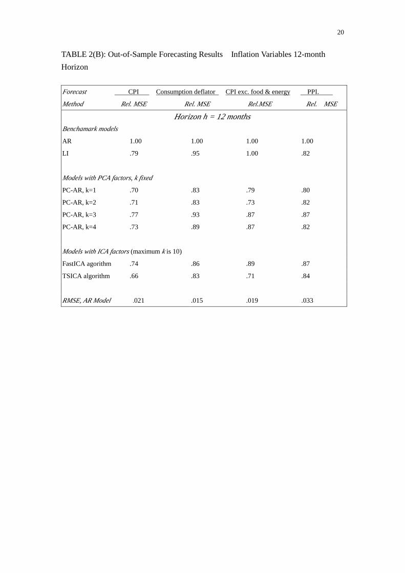
Tables 2(A), 2(B), and 2(C) report forecast results for price inflation variables. Stock

and Watson (2002) find that including autoregressive components in addition to PC can

dramatically improves the forecasts. That is, using ‘PC-AR” with fixed single PC factor can

12

yield the best performance. Using ICA technique somewhat has its payoff shown in these

tables. Model with TSICA algorithm perform a fine job in forecasting consumption deflator

(h=6 and 12), in forecasting no food and energy CPI (h=12 and 24) and in forecasting PPI

(h=6).

4 Conclusion

This paper has explored the possibility of using ICA technique to yield economic common

components from a large number of macroeconomic variables. The ICA method has been

regarded as a better method to separate sources that are non-Gaussian distributed and sta-

tistically independent to each other. However, in terms of forecasting the real activity, the

independent component method does not seem to demonstrate its advantage over the prin-

cipal component method. In forecasting inflation variable, in some cases, the ICA technique

shows its forecasting strength. Overall, the forecasting results comparing the ICA technique

with the PCA technique are mixing.

Possible extensions to this line of research are raised here. First, the dynamic factor

model considered in this paper is restricted to be linear. This leads to the possibility that a

nonlinear ICA-based model can generate forecasting gains. Second, the results reported here

are based on 146 series of the balanced panel. Will the ICA method produce better empirical

results when it is applied to a larger panel, such as the 215 full dataset? Particularly, when

the full dataset contains more outliers and data irregularity. Third, the transformation

applied to the raw data before estimating the IC factors may have produced too much noise

in the time series for the estimated factors to be accurate. One might want to estimate the

independent factors from the raw data directly and apply suitable filtering to smooth the

factors before he proceeds to forecast macroeconomic variables.

References

Bai, J. and S. Ng (2002). “Determining the number of factors in approximate factor mod-els.” Econometrica 70, NO. 1, 191-221.

13

Chamberlain, G. and M. Rothschild (1983). “Arbitrage factor structure and mean-varianceanalysis of large asset markets.” Econometrica 51, No. 5, 1305-1324.

Engle, R.F., and M.W. Watson (1981). “A one-factor multivariate time series model ofmetropolitan wage rates.” Journal of the American Statistical Association, 76, 774-781.

Forni, M. and L. Reichlin (1996). “Dynamic common factors in large cross-sections.” Em-pirical Economics, 21, 27-42.

Forni, M. and L. Reichlin (1998). “Lets get real: A dynamic factor analytical approach todisaggregated business cycle.” Review of Economic Studies 65, 453-474

Forni, M., M. Hallin, M. Lippi, and L. Reichlin (2000). “The generalized dynamic factormodel: Identification and estimation.” The Review of Economics and Statistics 82(4),540-552.

Geweke, J. (1977). “The dynamic factor analysis of economic time series.” in D.J. Aignerand A.S. Goldberger (eds.), Latent Variables in Socio-Economic Models, North-Holland,Amsterdam, Ch. 19.

Geweke, J. and K.J. Singleton (1981). “Maximum likelihood ’confirmatory’ factor analysisof economic time series.” International Economic review 22, 37-54.

Hyvarinen, A., J. Karhunen, and E. Oja (2001). Independent Component Analysis, JohnWiley & Sons, Inc., New York.

Hyvarinen, A. and E. Oja (1997). “A fast fixed-point algorithm for independent componentanalysis.” Neural Computation 9(7), 1483-1492.

Leeper, E.M., C.A. Sims and T. Zha (1996). “What does monetary policy do?” BrookingsPapers on Economic Activity.

Quah, D. and T.J. Sargent (983). “A dynamic index model for large cross sections.”In Business Cycles, Indicators, and Forecasting, eds. J.H. Stock and M.W. Watson,Chicago: University of Chicago Press, 285-306.

Sargent and Sims (1977). “Business cycle modeling without pretending to have too mucha-priori economic theory.” In New Methods in Business Cycle Research, ed. C. Simset al., Minneapolis: Federal Reserve Bank of Minneapolis.

Singleton, K.J. (1980). “A latent time series model of the cyclical behavior of interestrates.” International Economic Review 21, 559-575.

Stock, James H. and Mark W. Watson (2002). “Macroeconomic forecasting using diffusionindexes.” Journal of Business and Economic Statistics 20(2), 147-162.

14

Stock, James H. and Mark W. Watson (1989). “New indexes of coincident and leadingeconomic indicators.” NBER Macroeconomics Annual, 351-393.

Stock, J.H. and M.W. Watson (1998). “Diffusion indexes.” NBER Working Paper No.W6702.

Stock, James H. and Mark W. Watson (1999). “Forecasting inflation.” Journal of MonetaryEconomics 44, 293-335.

Watson, M.W. (2000). “Macroeconomic forecasting using many predictors.” Manuscript,Department of Economics and Woodrow Wilson School, Princeton University.

Econometrica 64, 1067-1084.

15

Figure1: R2 Between Factors and Individual Time Series, Grouped by Category.

16

TABLE 1(A): Out-of-Sample Forecasting Results：Real Variables 6-month Horizon

Forecast Industrial Production Personal Income Mfg & Trade sale Nonag. Employment

Method Rel. MSE Rel. MSE Rel.MSE Rel. MSE

Horizon h = 6 monthsBenchamark models

AR 1.00 1.00 1.00 1.00

LI .70 .83 .77 .75

Models with PCA factors, k fixed

PC, k=1 .88 .83 .93 .88

PC, k=2 .67 .77 .74 .91

PC, k=3 .66 .77 .69 .91

PC, k=4 .66 .77 .69 .91

Models with ICA factors (maximum k is 10)

FastICA agorithm 1.12 1.03 .83 .97

TSICA algorithm .92 .84 .75 .89

RMSE, AR Model .030 .016 .028 .008

17

TABLE 1(B): Out-of-Sample Forecasting Results：Real Variables 12-month Horizon




AR 1.00 1.00 1.00 1.00

LI .86 .97 .82 .89


PC, k=1 .94 .91 .94 .90

PC, k=2 .62 .81 .64 .83

PC, k=3 .55 .78 .59 .81

PC, k=4 .56 .81 .59 .84


FastICA agorithm 1.23 1.17 .78 1.03

TSICA algorithm 1.06 .89 .61 .94

RMSE, AR Model .049 .027 .045 .017

18

TABLE 1(C): Out-of-Sample Forecasting Results：Real Variables 24-month Horizon




AR 1.00 1.00 1.00 1.00

LI 1.09 1.29 1.08 1.07


PC, k=1 1.00 .99 .99 .92

PC, k=2 .77 .89 .71 .74

PC, k=3 .55 .71 .65 .67

PC, k=4 .56 .75 .66 .75


FastICA agorithm 1.40 1.11 .83 1.08

TSICA algorithm 1.19 .94 .70 .99

RMSE, AR Model .075 .046 .070 .031

19

TABLE 2(A): Out-of-Sample Forecasting Results：Inflation Variables 6-month Horizon

Forecast CPI Consumption deflator CPI exc. food & energy PPI.



AR 1.00 1.00 1.00 1.00

LI .82 1.04 1.10 1.00


PC-AR, k=1 .77 .89 .90 .88

PC-AR, k=2 .76 .89 .80 .89

PC-AR, k=3 .78 .93 .85 .91

PC-AR, k=4 .77 .93 .85 .90


FastICA agorithm .80 .88 .91 .86


RMSE, AR Model .010 .007 .009 .017

20

TABLE 2(B): Out-of-Sample Forecasting Results：Inflation Variables 12-month Horizon




AR 1.00 1.00 1.00 1.00

LI .79 .95 1.00 .82


PC-AR, k=1 .70 .83 .79 .80

PC-AR, k=2 .71 .83 .73 .82

PC-AR, k=3 .77 .93 .87 .87

PC-AR, k=4 .73 .89 .87 .82




RMSE, AR Model .021 .015 .019 .033

21

TABLE 2(C): Out-of-Sample Forecasting Results：Inflation Variables 24-month Horizon




AR 1.00 1.00 1.00 1.00

LI .70 .70 .99 .65


PC-AR, k=1 .66 .72 .66 .76

PC-AR, k=2 .66 .74 .66 .73

PC-AR, k=3 .74 .77 .87 .80

PC-AR, k=4 .70 .70 .87 .75




RMSE, AR Model .052 .038 .046 .077

macroeconomic forecasting with independent component - repec

Documents