Macroeconomic Inßuences on Optimal Asset

Allocation

T.J. Flavin

National University of Ireland, Maynooth

M.R. Wickens

University of York

March 2001

Keywords: Asset allocation, macroeconomic effects, multivariate GARCH

JEL ClassiÞcation: G11.

Address for correspondence: Dr. Thomas Flavin, Dept. of Economics,

NUI Maynooth, Co. Kildare, Rep. of Ireland. Tel. + 353 1 7083369; Fax:

+ 353 1 7083934; email: thomas.ßavin@may.ie

*The authors gratefully acknowledge the constructive criticisms offered by two

anonymous referees.

1

Macroeconomic Inßuences on Optimal Asset Allocation

Abstract

We develop a tactical asset allocation strategy that incorporates the ef-

fects of macroeconomic variables. The joint distribution of Þnancial asset

returns and the macroeconomic variables is modelled using a VAR with an

M-GARCH error structure. As a result the portfolio frontier is time varying

and subject to contagion from the macroeconomic variable. Optimal asset

allocation requires that this be taken into account. We illustrate the how to

do this using three risky UK assets and inßation as a macroeconomic factor.

Taking account of inßation generates portfolio frontiers that lie closer to the

origin, and offers investors superior risk-return combinations.

2

1 Introduction

This paper shows how macroeconomic information can be used to improve

asset allocation. Evidence on the use of Þnancial and macroeconomic vari-

ables to predict Þnancial asset returns, which is a burgeoning literature, is

not necessarily of most use for asset allocation. Indeed, we show that in-

formation about the volatility, not the level, of asset returns plays a more

signiÞcant role in portfolio selection models. The idea of this paper is to

exploit the time series structure of volatility contagion between Þnancial and

macroeconomic variables. If macroeconomic volatility can help predict the

volatility of asset returns then this can be used to improve tactical asset al-

location. This is done by relating the mean-variance portfolio frontier to the

macroeconomic factors.

Traditional methods of portfolio selection such as the mean-variance anal-

ysis of Markowitz (1952, 1959) and the CAPM due to Sharpe (1964) and

Lintner (1965) are based on the assumption of constant asset return volatil-

ity and hence a constant portfolio frontier. It has been noted by, for example,

Harvey (1991) that the covariance matrix of returns, from which the portfolio

frontier is formed, is in fact time varying. Ferson and Harvey (1997) exploit

this in their cross-section analysis of asset pricing. This implies that instead

of the portfolio frontier being based on the unconditional covariance matrix

of returns, which is constant, it should be calculated from the conditional

covariance matrix, which is time-varying.

This is the methodology used by Flavin and Wickens (1998) where it is

shown investors in UK assets could enjoy a signiÞcant reduction in portfolio

risk by employing a time-varying conditional covariance matrix instead of

3

a constant, unconditional covariance matrix to form the portfolio frontier.

As the frontier is also time varying, the portfolio needs to be continuously

re-balanced. Financial asset returns were conditioned on past realised values

using a multivariate GARCH(1,1) process to model the volatility contagion.

We extend this methodology to take account of macroeconomic variables.

By modelling the asset returns jointly with the macroeconomic variables, we

can assess and take account of the inßuence of the macroeconomic variables

on both the conditional mean and the conditional covariance matrix of the

asset returns. The resulting time-varying conditional covariance matrices

are then used to develop a tactical asset allocation strategy in which individ-

ual asset holdings are continuously updated in response to changes in their

perceived riskiness which are due in part to macroeconomic effects. In this

illustration, we consider only one macroeconomic variable, inßation.1

In order to help determine the additional beneÞts of taking account of

macroeconomic effects we build on the analysis of Flavin and Wickens (1998)

who examine three UK risky assets: equity, a long government bond and

a short-term bond. We Þnd that inßation exerts a strong inßuence on the

volatility of these asset returns and on the shape and location of the portfolio

mean-variance frontier. As a result of taking account of inßation effects, we

Þnd that for portfolios for which the asset shares are restricted to be non-

negative, the optimal share of equities increases from 70% to 74%, the share

of the long bonds share falls from 20% to 14% and the share of the short

1The extension of portfolio analysis to take account of macroeconomic volatility conta-

gion, even of one variable, is a non-trivial issue. For example, in a recent paper on variable

selection for portfolio choice Ait-Sahalia and Brandt (2001) conÞne their selection to just

Þnancial asset returns.

4

bond increases from 10% to 12%. These are signiÞcant changes.

The paper is structured as follows; section 2 reviews the literature on the

relation between macroeconomic variables and the returns and volatility of

Þnancial assets. Section 3 explains how to take account of macroeconomic

factors in asset allocation. Section 4 presents the econometric model of the

joint distribution of returns and the macroeconomic variable. Our choice of

the macroeconomic variable and a description of the data is given in Section 5.

The estimates of the econometric model are reported in Section 6. Section 7

contains an analysis of the portfolio frontier and the optimal asset shares both

ignoring and taking account of the inßuence of inßation. Our conclusions are

reported in Section 8.

2 Asset Returns and Macroeconomics

There are good theoretical reasons to believe that macroeconomic variables

affect asset returns. If returns are deÞned in nominal terms, and investors

are concerned with real returns, then we would expect that nominal returns

would fully reßect inßation in the long term, though how much of this is

transmitted in the short term is still unclear. As a result, stocks should

prove to be an effective hedge against inßation ex post. Changes in inßation

expectations are also thought to be a major factor in determining the shape

of the yield curve. General equilibrium models of asset price determination

relate nominal asset returns to consumption, as well as inßation.

Since the mid-1980s there has been a growing literature on empirical ev-

idence of the information contained in macroeconomic variables about asset

5

prices. Most of this research is, however, about predicting Þnancial asset

returns, and very little is about forecasting asset price volatility. We brießy

review some of this literature, and then turn to the evidence on the macroe-

conomic inßuences on asset price volatility.

2.1 Asset Returns

In this review we focus mainly on evidence about the usefulness of macroe-

conomic variables in predicting stock returns. Similar factors seem also to

affect bond markets. Fama and French (1989) provide evidence that forecasts

of excess bond and stock returns are correlated, while Campbell, and Ammer

(1993) Þnd that variables which are useful in forecasting excess stock returns

can also predict excess bond returns.

Chen et al. (1986) are credited with being the pioneers in the asset return

predictability literature following their paper identifying factors that can be

potentially used to predict US stock market prices. They found that the fol-

lowing are all signiÞcantly priced in the US stock market: the spread between

long-term and short-term interest rates (a measure of the term structure or

slope of the yield curve), expected and unexpected inßation, industrial pro-

duction, and the spread between high- and low-grade bonds. Jankus (1997)

shows that expected inßation is also a useful predictor of future bond yields.

In a similar vein, many papers provide evidence of the explanatory power

of the dividend yield over annual US stock returns (Rozeff (1984), Campbell

and Shiller (1988), Hodrick (1992), Patelis (1997) etc.). A positive correla-

tion between the term structure of interest rates and stock price movements

has been documented for the US (Keim and Stambaugh (1986), Campbell

6

(1987), Patelis (1997)) while the slope of the term structure is found to

have forecasting power for excess bond returns in, for example, Campbell

and Shiller (1991), Fama (1984) and Tzavalis and Wickens (1997). Using

cross-sectional data, Fama and French (1992,1995) Þnd support for a nega-

tive relation between Price/Book ratio and US stock returns. Peseran and

Timmermann (1995) identify many factors that can inßuence returns on US

equities. These include the earnings-price ratio, the rates of return on one-

and twelve-month Treasury bills, the change in domestic inßation, the change

in industrial production, and monetary growth.

A parallel literature has emerged in the UK. Clare et al. (1993) show

that the Gilt to Equity Yield Ratio (GEYR) contains predictive power over

UK stock price movements. Clare and Thomas (1994) Þnd that the current

account balance, US equity, German equity, the 90-day UK Treasury bill

rate, the differential between the 90-day UK and US Treasury bill rates; the

irredeemable government bond index, the corporate bond index, the term

structure of interest rates, and the dollar to pound exchange rate are all

signiÞcantly priced in the UK stock market. Clare et al. (1997) focus on the

ability of lagged own values and lagged values of returns on other markets

to predict UK stock returns.

Asprem (1989) conducted a wide ranging analysis of the relation between

stock market indices, portfolios of assets and macroeconomic phenomena in

ten European countries. Interestingly, he Þnds that the linkages between

stock prices and macroeconomic variables are most pronounced in Germany,

the Netherlands, Switzerland and the UK. For these countries, he Þnds strong

evidence of a negative relation between stock prices and current and lagged

7

values of the interest rate. Furthermore, current values of the US term struc-

ture of interest rates are found to have signiÞcant explanatory power over

stock returns in these countries. Consistent with other studies, he Þnds that

asset prices and inßation are negatively correlated. This relation appears to

hold both for past as well as expected future changes in inßation.

Since money supply growth and inßation are positively linked through

the quantity theory of money, we would expect a similar relation between

money growth and stock prices. Using the monetary base, M0, as a measure

of money supply, Asprems evidence indicates a negative correlation. Only

for the UK is this relation statistically signiÞcant. He Þnds that many other

variables are not signiÞcantly related to stock prices, including measures of

real economic activity, (trade-weighted) exchange rates and, with the excep-

tion of the UK, consumption.

2.2 Asset Return Volatility

In contrast to this wealth of evidence on the predictability of the level of

asset returns, little attention has been paid in the literature to the ability of

macroeconomic variables to inßuence asset price volatility.

Historically, Þnancial market turbulence has been greatest in times of

recession (see Schwert (1989)) and recent evidence suggests that stock mar-

ket volatility is related to the general well-being of the economy. Clarke

and De Silva (1998) report that state-dependent variation in asset returns

has strong implications for identifying an optimal asset allocation strategy,

while Klemkosky and Bharati (1995) show that short-term predictability can

be used to build proÞtable asset allocation models.

8

In a test of the international CAPM, Engel and Rodrigues (1989) al-

low macroeconomic variables to inßuence the variance process of an ARCH

model. They Þnd that the square of the unanticipated monthly growth rate

of dollar oil prices and the monthly growth rate of US M1 are signiÞcant

explanatory variables of the variance of residuals. Clare et al. (1998) demon-

strate that when a number of macroeconomic variables are subjected to si-

multaneous shocks, they can have a signiÞcant inßuence on the conditional

covariance matrix of excess returns. Wickens and Smith (2001) examine the

macroeconomic inßuences on the sterling-dollar exchange rate that arise from

general equilibrium and other models.

In summary, there is strong evidence that a broad range of macroeconomic

factors are signiÞcantly priced in global stock markets. Changes in inßation

(both realised and expected), interest rates, imports, consumption tend to be

negatively correlated with stock returns, and bond yields tend to be positively

related with stock returns. In contrast, to these Þndings for returns, much

less attention has been paid to the inßuence of macroeconomic variables on

the variances and covariances of returns. As this is crucial for optimal asset

allocation, this is what we focus on.

3 Optimal Asset Allocation

Standard portfolio theory based on mean-variance analysis or CAPM assumes

a constant covariance matrix of asset returns. In principle it is straightfor-

ward to extend this to a time-varying, or conditional, covariance matrix of

returns, see for example Cumby et al. (1994), or Flavin and Wickens (1998).

9

As a result, the mean-variance portfolio frontier also becomes time varying

and optimal asset allocation requires a continuous re-balancing of portfolio

shares.

The asset shares can be unrestricted, or constrained to be non-negative

to avoid short sales which may be prohibited for legal reasons. This is a

situation facing a large number of fund managers, for example, UK pension

funds. To aid comparisons between unconstrained and constrained asset

allocations, the target rate of return when asset shares are constrained can

be taken to be the average return on the unconstrained optimal portfolio.

To take account of the effect of macroeconomic variables on asset allo-

cation, a further extension is required. This is achieved by augmenting the

vector of excess returns with the macroeconomic variables, after suitably

transforming them to stationarity where necessary. The joint distribution of

this augmented vector, allowing for time-varying conditional heteroskedas-

ticity in all variables is then required. The conditional covariance matrix of

excess returns of this joint distribution is formed from the resulting multivari-

ate marginal conditional distribution of the excess returns. The conditional

distribution of excess returns will depend on the volatility of the macroeco-

nomic variables, which can be used to help predict the covariance matrix of

the excess returns and hence the portfolio frontier. The construction of the

optimal portfolio is now obtained as before, but the asset shares will differ

from those computed without taking account of the contagion effects from

the macroeconomic variables.

10

4 Econometric Issues

4.1 Model

The joint distribution of the Þnancial and macroeconomic variables is speci-

Þed through an econometric model. We employ a multivariate GARCH(1,1)

- i.e. M-GARCH(1,1) - model of excess returns. This has a time-varying

covariance matrix.

GARCH models are widely used in Þnancial econometrics. For asset allo-

cation it is necessary to use M-GARCH as the joint distribution of returns is

required. Unfortunately, it is often difficult to estimate M-GARCH models

due to dimensionality problems arising from the vast number of potential pa-

rameters to be estimated simultaneously. For example, for the most general

formulation of the M-GARCH(1,1) model, termed the vec representation by

Baba, Engle, Kraft & Kroner (1990) - or BEKK - the number of parameters

to be estimated increases at the rate of n4, where n is the number of vari-

ables. Thus, although in principle, for portfolio analysis, one would like a

model capable of handling a large number of assets simultaneously, and with

a structure ßexible enough to capture the dynamic and leptokurtic charac-

teristics of the distribution of asset returns, in practice, this choice is severely

limited by numerical problems. We overcome this shortcoming by adopting

the parameterisation of the Flavin and Wickens (1998).2 This formulation is

better suited to portfolio analysis in that it allows a considerable degree of

ßexibility in the conditional covariance matrix of returns yet is economical

2This parameterisation is consistent with the covariance stationary model developed in

Engle and Kroner (1995).

11

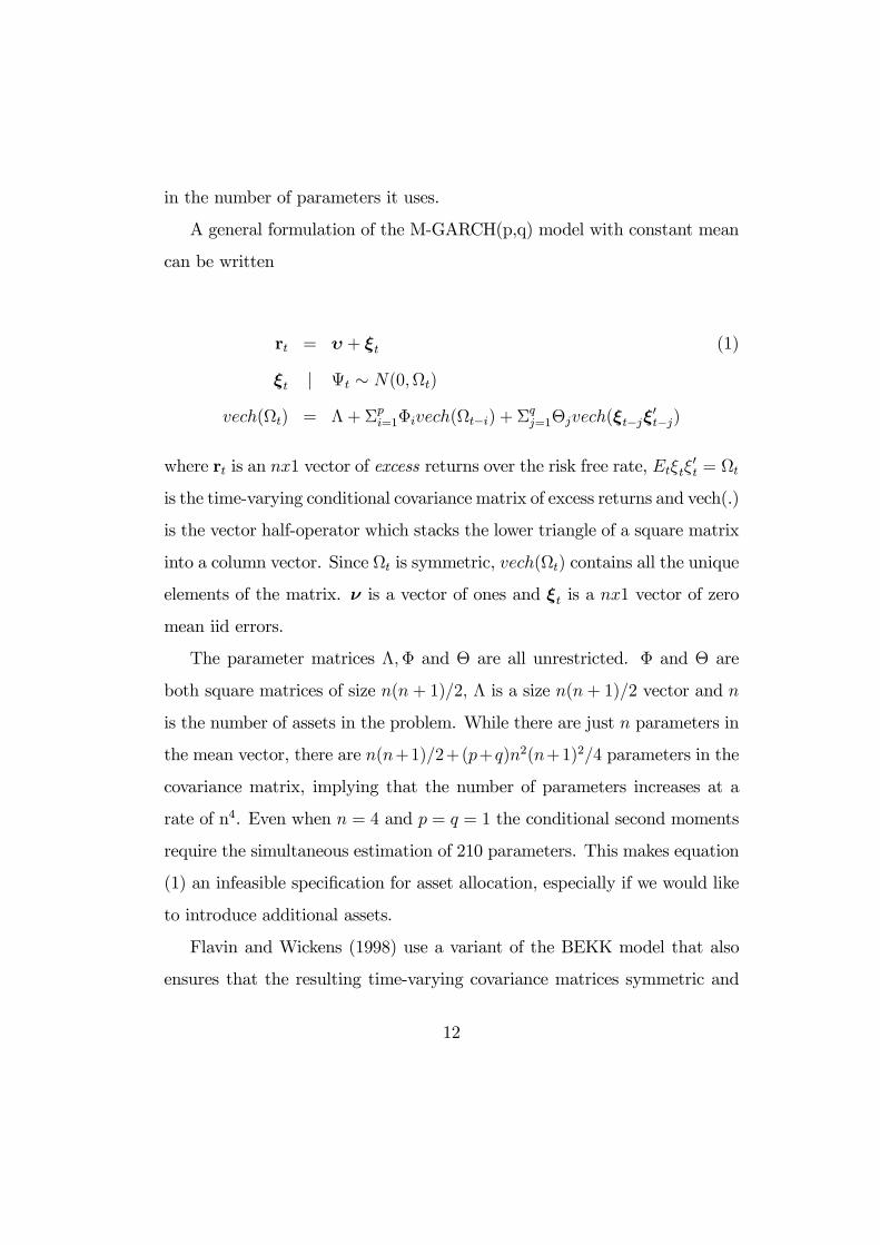
in the number of parameters it uses.

A general formulation of the M-GARCH(p,q) model with constant mean

can be written

rt = υ + ξt (1)

ξt | Ψt ∼ N(0,Ωt)vech(Ωt) = Λ+ Σpi=1Φivech(Ωt−i) + Σ

qj=1Θjvech(ξt−jξ

0t−j)

where rt is an nx1 vector of excess returns over the risk free rate, Etξtξ0t = Ωt

is the time-varying conditional covariance matrix of excess returns and vech(.)

is the vector half-operator which stacks the lower triangle of a square matrix

into a column vector. Since Ωt is symmetric, vech(Ωt) contains all the unique

elements of the matrix. ν is a vector of ones and ξt is a nx1 vector of zero

mean iid errors.

The parameter matrices Λ,Φ and Θ are all unrestricted. Φ and Θ are

both square matrices of size n(n+ 1)/2, Λ is a size n(n+ 1)/2 vector and n

is the number of assets in the problem. While there are just n parameters in

the mean vector, there are n(n+1)/2+(p+q)n2(n+1)2/4 parameters in the

covariance matrix, implying that the number of parameters increases at a

rate of n4. Even when n = 4 and p = q = 1 the conditional second moments

require the simultaneous estimation of 210 parameters. This makes equation

(1) an infeasible speciÞcation for asset allocation, especially if we would like

to introduce additional assets.

Flavin and Wickens (1998) use a variant of the BEKK model that also

ensures that the resulting time-varying covariance matrices symmetric and

12

positive deÞnite.3. The Φ and Θ matrices in equation (1) are diagonalised

and the ijth element of the covariance matrix is inßuenced by its own lagged

value and past values of ξiξj only. As in Flavin and Wickens (1998), we also

specify the time-varying covariance matrix in error correction form. This

has the advantage of separating the long-run from the short-run dynamic

structure of the covariance matrix.

Augmenting the vector of asset returns with a vector of macroeconomic

variables gives

zt = α+ βzt−1 + γdum87 + ξt (2)

ξt | Ψt−1 ∼ N(0,Ht)

Ht = V0V +A0(Ht−1 −V0V)A+B0(ξt−1ξ

0t−1 −V0V)B, (3)

where z = (r,m)0. In this study r = (ukeq, lbd, sbd)0, ukeq, lbd and sbd

represent the excess returns on UK equity, long government bonds and short

government bonds respectively, and m is a single macroeconomic factor, the

change in domestic inßation. Thus inßation is constrained to have no effect

on excess returns in the long run. More generally both r and m will be

vectors. dum87 is a dummy variable for the October 1987 stock market

crash and is included only in the equity equation of the model.

The Þrst term on the right-hand side of equation (3) is the long-run, or

unconditional, covariance matrix. The other two terms capture the short-

run deviation from the long run. By formulating the conditional variance-

covariance structure in this way, we can decide more easily if the short-run

3For a discussion of this and a review of alternative speciÞcations, see Bollerslev, Engle

& Nelson(1994) and Bera & Higgins(1993).

13

dynamics have a useful additional contribution to make, and if the increased

generality a parameter offers is worth the additional computational burden.

The speed with which volatility in the macroeconomic variables affect the

volatility of excess returns is an important issue. This is governed, in part,

by the choice of the A and B matrices. For example, if A and B are deÞned

as lower triangular matrices then, partitioning conformably with z = (r,m)

implies that

H11,t = V211 +A

211H11,t−1 +B211ε

21,t−1 (4)

and

ε1,t−1 = rt−1 − c1 − βrt−2 − δmt−2 (5)

Thus, the volatility of excess returns is unaffected by the volatility of the

macroeconomic variable.

Alternatively, if A and B are deÞned as full symmetric matrices then

H11,t = V211 +

(A211H11,t−1 + 2A11A12H12,t−1 +A212H22,t−1) + (6)

(B211ε21,t−1 + 2B11B12ε1,t−1ε2,t−1 +B

212ε

22,t−1)

In equation (6) volatility in the macroeconomic variable is transmitted to the

volatilities of the excess returns, but with a one period lag. This second for-

mulation is therefore clearly preferable and it is what we use. V is speciÞed,

without loss of generality, as a lower triangular matrix.

In general, asset returns and macroeconomic variables could have both a

time-varying conditional mean and covariance matrix. The evidence, how-

ever, is that excess equity and bond returns over the risk-free rate are almost

14

serially independent and hence are difficult to predict. Moreover, inßation

will have less effect on excess than straight returns even though, as explained

above, in the long run it can be expected to affect the rates of return on

equity and bonds one-for-one. Nevertheless, the effect in the short run re-

mains unclear, and is the reason we allow for the short-run effects of inßation

in our econometric model. Thus, unlike equation (1), equation (2) also al-

lows for a time-varying conditional mean and is therefore a VAR(1) in the

conditional mean with disturbances that are normally distributed with mean

zero and a time-varying variance-covariance matrix that is generated by an

M-GARCH(1,1) process.

The right-hand side of equation (2) can be interpreted as the implied

measure of (or proxy for) the risk premia. Optimum portfolio allocation, with

its focus on the conditional covariance matrix, can therefore be interpreted

as being based on the risk-neutral distribution.

4.2 Method of Estimation

Our model as speciÞed in equations (2) and (3) was estimated by maximising

the log likelihood function

LogL = −nT2log(2π)− 1

2

Xt

(log | Ωt | −ξ0t+1Ω−1t ξt+1) (7)

recursively using the Berndt, Hall, Hall & Hausmann (BHHH) algorithm. n

is the size of z and T is the number of observations.

15

5 Data issues

5.1 Choice of Macroeconomic Variables

In principle, many macroeconomic variables could be included in our analysis.

We restrict our analysis to one variable, inßation, for several reasons. Partly,

it is due to the dimensionality problem and because this paper is designed

to illustrate the methodology. Firstly, the choice of inßation is because, as

noted above, if investors seek real returns then they will want to be fully

compensated for inßation. It has also been argued by Schwert (1989) that

if the inßation of goods prices is uncertain, then the volatility of nominal

asset returns should reßect inßation volatility. Second, the empirical evidence

reviewed above is supportive of a strong relation between inßation and stock

and bond returns. Third, empirical evidence on the relation between inßation

and stock returns has produced something of a puzzle which has attracted

much attention. Theory suggests that the relation between nominal asset

returns and inßation would be positive but the empirical evidence usually

Þnds the relation between stock returns and inßation is consistently negative

across countries and over different time periods - see Bodie (1976) and Fama

and Schwert (1977) for the US and Solnik(1983) and Gultekin (1983) for a

number of other countries.4

In choosing a suitable inßation variable, we were faced with the choice of

a realised variable or an expectations variable. While both have been shown

to have predictive power over US stock returns, most research on UK stock

4Possible explanations of the puzzle have been offered by Nelson (1976), Fama (1981),

Geske and Roll (1983) and Groenewold et al. (1997).

16

returns has focussed on inßation measures based on the Retail Price Index

(see Asprem (1989) and Clare and Thomas (1994)). This measure is mostly

likely to be priced into UK stock returns as this rate is most often used as the

headline rate by UK market participants. Consequently, we use a realised

variable in the results reported below.5

5.2 Data

We include three risky UK Þnancial assets. These are equities, a long gov-

ernment bond and a short government bond. Equity is represented by the

Financial Times All Share Index, long government bonds are represented by

the FT British government stock with over 15 years to maturity index; and

short government bonds are represented by the FT British government stock

with under 5 years to maturity index. Each is expressed as an excess return

over the risk-free rate as proxied by the 30-day Treasury bill rate. The data

used are monthly total annualised returns.6 The inßation rate is calculated

from the UK Retail Price Index. As econometric tests fail to reject the null

hypothesis of a unit root in inßation, the change in inßation is used to en-

sure that all variables are stationary.7 The data are from January 1976 to

5Using a WPI based inßation measure yielded parameters of the same sign and similar

magnitude but many had reduced statistical signiÞcance.6Given that we use excess returns, we were faced with the question of annualising stock

returns or de-annualising the risk-free rate. In trying to achieve convergence in the M-

GARCH model, it is better to work with annualised data rather than the smaller numbers

associated with monthly returns. This is also the approach of Cumby et al. (1994).7Unit root tests were conducted on all variables and results are available from the

authors.

17

September 1996 and were sourced from DATASTREAM.

6 Results

6.1 Conditional Mean

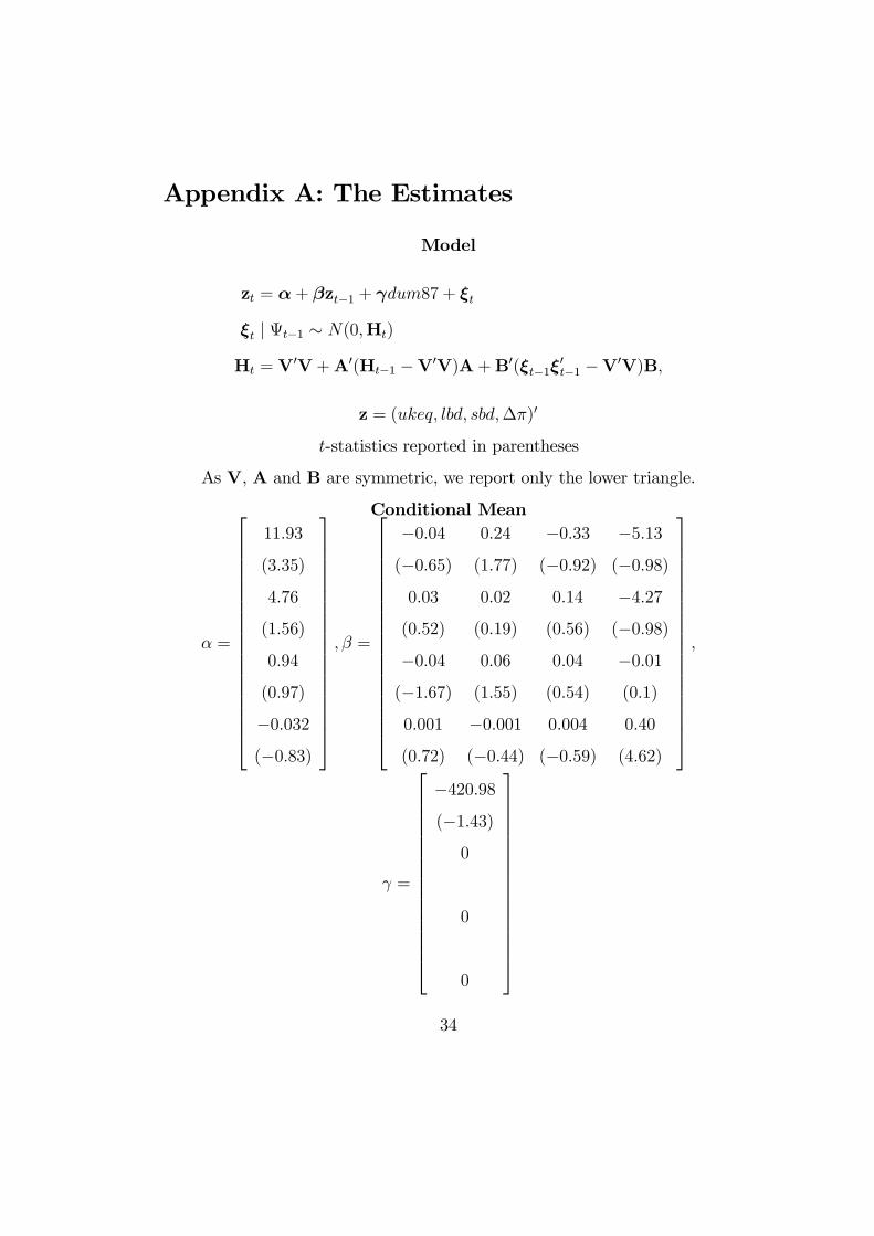
Our estimates are reported in Appendix A. The estimates of the conditional

mean broadly conÞrm that excess returns are unpredictable using this infor-

mation set. The only signiÞcant coefficient in the β matrix is in the inßation

equation, and it is for the lagged change of inßation. In the intercept vector

α the only signiÞcant coefficient is for equity. This is consistent with having

a substantial equity premium. The intercept for the excess returns on long

bonds is quite large, but is not well determined.

When selecting Þnancial asset portfolios, we use a vector of historical

means as our proxy for expected returns. This approach has been advocated

by Jobson and Korkie (1981) who demonstrate that this greatly improves

portfolio performance. It is also argued in Flavin and Wickens (1998) that

this approach is preferable given the insigniÞcance of the estimated parame-

ters in the mean equation already mentioned. As well as being expensive in

terms of transaction costs, re-balancing our portfolio in response to changes

in the predicted excess return would also be counter-productive due to the

lack of persistence of the deviations of excess returns from their unconditional

means. This is not true of re-balancing due to changes in the conditional vari-

ance because of their much higher degree of persistence and lower volatility.

18

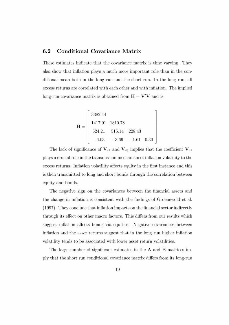
6.2 Conditional Covariance Matrix

These estimates indicate that the covariance matrix is time varying. They

also show that inßation plays a much more important role than in the con-

ditional mean both in the long run and the short run. In the long run, all

excess returns are correlated with each other and with inßation. The implied

long-run covariance matrix is obtained from H = V0V and is

H =

3382.44

1417.91 1810.78

524.21 515.14 228.43

−6.03 −3.69 −1.61 0.30

The lack of signiÞcance of V42 and V43 implies that the coefficient V41

plays a crucial role in the transmission mechanism of inßation volatility to the

excess returns. Inßation volatility affects equity in the Þrst instance and this

is then transmitted to long and short bonds through the correlation between

equity and bonds.

The negative sign on the covariances between the Þnancial assets and

the change in inßation is consistent with the Þndings of Groenewold et al.

(1997). They conclude that inßation impacts on the Þnancial sector indirectly

through its effect on other macro factors. This differs from our results which

suggest inßation affects bonds via equities. Negative covariances between

inßation and the asset returns suggest that in the long run higher inßation

volatility tends to be associated with lower asset return volatilities.

The large number of signiÞcant estimates in the A and B matrices im-

ply that the short run conditional covariance matrix differs from its long-run

19

level. Roughly speaking, and ignoring the other elements, the greater the

elements on the leading diagonals of A and B, the more the conditional co-

variance matrix deviates from the long-run value. The off-diagonal elements

contribute to the contagion effects in the short run. These estimates suggest

that the deviations from the long-run covariance matrix are both persistent

and predictable.

Figure 1 depicts the long-run variances and the short-run conditional

variances of the three excess asset returns. The short-run deviations are

clearly substantial. The conditional variances are usually below their long-

run value (especially for equity and the short bond). This suggests that for

much of the time investors can hold more equity and short-run bonds than

use of the long-run covariance matrix would imply.

The impact of inßation volatility on short-run asset return volatility is

very important, especially for the long bond, as both B42 and A42 are statis-

tically signiÞcant. Inßation volatility also affects the short-run volatility of

UK equity as B41 and A41 are marginally signiÞcant. The short bond seems

to be least affected even though there is evidence of signiÞcance in the A43

parameter.

Viewed as a whole, these results show that while asset returns are close

to being unpredictable, asset return volatility is time-varying, persistent and

much more predictable. They offer considerable support for taking account

of inßation in explaining the volatility of asset returns, and the preliminary

indication is that the optimum portfolio allocation may involve holding more

equity than the portfolio allocation based on a constant volatility would

suggest. We now examine the implications for asset allocation in more detail.

20

7 Portfolio Selection

7.1 The Portfolio Frontier

As explained earlier, to form optimal portfolios, we require the conditional

covariance matrix of the joint marginal distribution of the excess asset re-

turns. To obtain this, we simply partition conformably with the sub-vector

of asset returns. Next we generate the time-varying minimum-variance port-

folio frontiers using historical returns as a proxy for expected returns. The

time variation in the conditional covariance matrix of returns is reßected in

the time variation in the frontiers, and implies that portfolios will need to be

continuously rebalanced to be optimal.

Figure 2 shows the distribution of frontiers generated over the entire 20

year sample. The range of movement is quite large and the shape changes

too. For the minimum-variance portfolios, the minimum standard deviation

of the portfolio is about 6% and the maximum is roughly 22%.

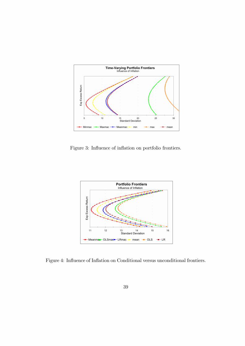
It is instructive to compare these frontiers with those obtained by Flavin

and Wickens (1998), which take no account of the macroeconomic factor.

These are displayed in Figure 3. In general, taking account of inßation results

in the whole distribution of mean-variance frontiers shifting to the left, and a

more negatively skewed distribution as while the mean is little changed, the

minimum and the maximum frontiers are shifted to the left. A possible reason

why the mean portfolio frontiers are similar is that by omitting inßation from

the econometric model, in effect the bias introduced is evaluated at the mean

level and long-run variance of inßation. This shift to the left in the frontier

is due mainly to the negative conditional covariance between equity excess

21

returns and inßation. It implies that investors can achieve a higher expected

return for any given level of risk, or lower risk for any given level of return.

Figure 4 tells a similar story. It depicts the mean frontiers obtained in a

number of different ways. The left-most frontier is the optimal frontier based

on taking full account of inßation. Moving to the right, the next frontier

ignores inßation. The third and fourth frontiers are based on the respective

long-run solutions of these two approaches. These use V0V instead of the

conditional covariance matrices. The Þnal two frontiers have been computed

from a simple OLS estimate of the unconditional covariance matrix of excess

returns. These results show the beneÞts of taking account of inßation and

of using an estimate of the conditional covariance matrix. They also show

that even if the constant long-run covariance matrix is used, it is better to

estimate this from the short-term model.

7.2 Portfolio Selection

We consider three types of portfolio, the minimum-variance portfolio (MVP),

the optimal unconstrained portfolio (OUP) and the optimal constrained port-

folio (OCP). All three take account of the inßuence of inßation and are based

on holding only risky assets. The two latter portfolios represent the optimal

portfolio of risky assets and based on CAPM would be held together with a

risk-free asset. However, we identify the constituents of the risky portfolio

and leave the Þnal investment position to the individual. The OUP allows

the portfolio weights to be negative, and hence permits short sales, and the

OCP is restricted to have non-negative weights. The location of the OUP

can be represented as a point on the tangent from the portfolio frontier to

22

the risk-free rate of interest. The OCP not only restricts the asset shares to

be non-negative, it is also constrained to have the average return on the un-

restricted portfolio. In this way investors are not penalised by the restriction

on the shares, and it aids comparisons with the unrestricted case. The OCP

requires the use of quadratic programming.

7.2.1 Unrestricted Weights

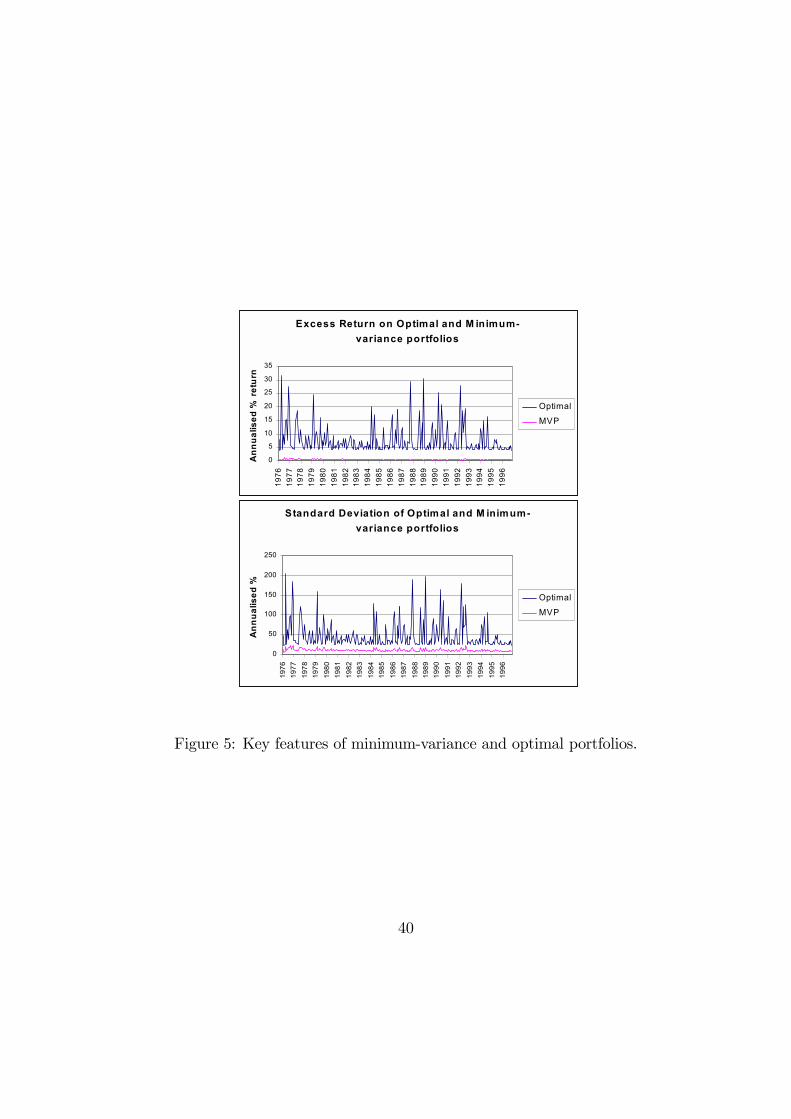
Figure 5 plots the excess return and standard deviation of the minimum-

variance portfolio and the OUP. Whilst the return on the OUP is always

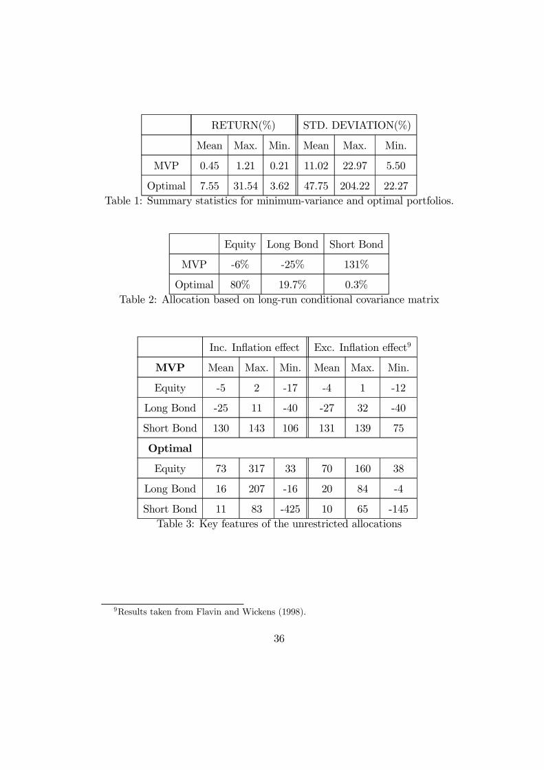
higher than that of the MVP, so is the standard deviation. Table 1 provides

a summary of the key features of these portfolios.

A common measure of overall portfolio performance is the Sharpe Per-

formance Index which is deÞned as SPI = excess rtnrisk

. In Figure 6 we report

the SPI for the OUP both with and without taking account of inßation.

We only compute the SPI for the OUP as this is higher than those for the

MVP. The two portfolios have similar SPI values. This is consistent with

the convergence of the frontiers in the efficient region. The mean values are

about 0.16.

The average asset shares for the MVP and the OUP are reported in

Table 2.8 They are strikingly different. Whereas the MVP is dominated by

the short bond and equity is sold short, the OUP is dominated by equity and

the share in the short bond is miniscule. Figures 7 and 8 plot the shares for

the two portfolios and Table 3 presents summary statistics. For the MVP

8These weight vectors are computed using standard results for portfolio mathematics

(see Huang and Litzenberger (1988)).

23

the shares are very stable across time. The short bond always accounts for

more than 100% of wealth and is funded mainly by a short position in the

long bond, though equity is also predominantly held short. The inclusion of

the inßation innovation has not greatly altered the share of asset holdings,

but it has dampened the volatility in bond holdings.

In the OUP equity dominates, on average accounting for 73% of the

portfolio. It is never held short and its share is often in excess of 100% of

wealth. One or both of the bonds are then held short to make this investment

possible. Comparing the OUP shares with those found by Flavin andWickens

(1998) which do not take account of inßation, the holdings of bonds are more

volatile, the mean holding of the long bond is reduced from 20% to16% (see

Table 3) and the investor holds bonds short on many more occasions. The

short government bond is still the most volatile asset, ranging from -425% to

83% of investor wealth, but its mean holding has remained largely unaltered

with only a slight increase from 10% to 11%. This would seem to be due

to the smaller inßuence of inßation on the volatility of the short government

bond as inßation may be more predictable at shorter horizons and hence not

as great a source of uncertainty as the short asset.

7.2.2 Restricted Weights

The OCP removes some of the undesirable features of the OUP, in partic-

ular the volatility of asset shares. It also eliminates short sales. Figure 9

shows that equity dominates the OCP in every period, and the share is quite

stable around the average position of 74% of the portfolio. The long bond

continues to dominate the short bond, but this is not as pronounced as in

24

the unrestricted allocation. The mean holdings of the long and short bonds

are 14% and 12% of the portfolio respectively. Table 4 summarises the asset

holdings under this investment strategy.

Table 5 compares these OCP shares with those of Flavin and Wickens

(1998) that do not take account of inßation. There is an increase in the

share of both equity (from 70% to 74%) and the short-term bond (from 10%

to 12%). These increases are offset by a reduction in the holding of the long

bond (from 20% to 14%). The increase in equity again reßects the negative

correlation of excess equity returns with inßation.

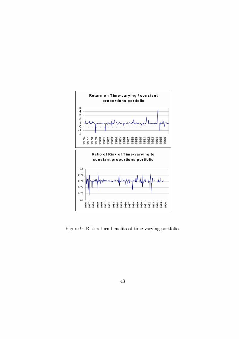
7.3 Portfolio Performance

To further help determine whether the effort involved in taking of account of

inßation has improved portfolio performance, we compare the OCP with a

portfolio with constant asset shares equal to the average weights for the OUP

reported in Table 2. In Figure 10 we plot the ratios of the expected return

and the standard deviation on the OCP to the constant proportions OUP.

The main difference lies in the riskiness of the portfolios. In every period

the risk associated with the OCP is much lower - on average by almost 24%.

The OCP has a lower average return, but the ratio is close to unity most of

the time.

We also compare the realised return and the realised volatility of returns

from the OCP with those from the constant shares portfolio. We Þnd that

the OCP has a slightly lower return - as above - but is compensated by a

lower realised volatility. This is evidenced by an increase of 1.6% in the

Sharpe Performance Index.

25

We conclude, therefore, that the greatest beneÞt of this approach to asset

allocation lies in its potential to reduce portfolio risk. This Þnding should

further encourage fund managers to adopt this asset allocation strategy.

8 Conclusion

In this paper we have described a way to take account of macroeconomic

factors in tactical asset allocation. The methodology is based on an exten-

sion of standard CAPM in which the minimum-variance portfolio frontier is

allowed to vary over time and to reßect variations in macroeconomic factors.

Flavin and Wickens (1998) show that a tactical asset allocation strategy that

involves continuously re-balancing a portfolio in response to changes in the

conditional covariance matrix permits a large reduction in risk over and above

a portfolio based upon a constant covariance matrix. We have shown here

that extending this analysis to allow for the incorporation of macroeconomic

variables in determining the covariance matrix of returns allows further sig-

niÞcant gains in risk reduction.

Our analysis which, is illustrative of the methodology, involves four Þ-

nancial returns (three risky assets and a risk-free asset), one macroeconomic

variable (inßation), and is for the UK. The risky assets are UK equity, a

long-term UK government bond and a short-term UK government bond.

The risk-free asset is the 30-day Treasury bill.

A crucial feature of the analysis is the ability to estimate the joint dis-

tribution of the excess returns and the macroeconomic factors to allow for

a time-varying covariance structure to the distribution. This permits the

26

macroeconomic factors to continuously inßuence the covariance matrix of

asset returns and hence the portfolio frontier formed from the covariance

matrix of the marginal joint distribution of returns. We employed a multi-

variate GARCH(1,1) model, but other models could be used.

We have found that inßation has a signiÞcant impact on the conditional

covariance matrix of asset returns. The transmission mechanism seems to be

via its effect on the volatility of equity. Inßation is negatively correlated with

all three excess returns in the long run, but the long-run impact is greatest

on equity; the impact on bonds is predominantly a short-run phenomenon.

The negative covariance between inßation and the excess returns generates

a signiÞcant reduction in portfolio risk over and above what can be achieved

by using a time-varying covariance matrix of excess returns alone. The risk

of the time-varying portfolio is at least 20% lower than that of the constant

proportions portfolio. There is also an improvement in overall portfolio per-

formance as measured by the SPI with the reduction in portfolio volatility

more than offsetting a lower realised average return. The unconstrained port-

folio has highly volatile shares, but the constrained portfolio is reasonably

stable. The average optimal constrained portfolio shares are: equity 74%,

the long bond 14%, and the short bond 12%.

27

References

[1] Ait-Sahalia,Y. and M.W.Brandt (2001). Variable selection for portfolio

choice. Journal of Finance, 56, 1297-1351.

[2] Asprem, M. (1989). Stock Prices, Asset Portfolios and Macroeconomic

Variables in Ten European Countries. Journal of Banking and Finance,

13, 589-612.

[3] Baba, Y., R.F. Engle, D.F. Kraft and K.F. Kroner (1990). Multivariate

Simultaneous Generalized ARCH. Mimeo, Dept. of Economics, Univer-

stity of California at San Diego.

[4] Bera, A.K. and M.L. Higgins (1993). ARCH Models: Properties, Esti-

mation and Testing. Journal of Economic Surveys, 7, 305-366.

[5] Berndt, E.R., B.H. Hall, R.E. Hall and J.A. Haussman (1974). Estima-

tion and Inference in Nonlinear Structural Models. Annals of Economic

and Social Management, 4, 653-665.

[6] Bodie, Z. (1976). Common Stocks as a hedge against Inßation. Journal

of Finance, 31, 459-470.

[7] Bollerslev, T., R.F. Engle and D.B. Nelson, (1994). ARCH Models. In

Handbook of Econometrics, edited by R.F. Engle & D.L. McFadden,

Elsevier Science B.V.

[8] Campbell, J.Y. (1987). Stock Returns and the Term Structure. Journal

of Financial Economics, 18, 373-399.

28

[9] Campbell, J.Y.and J. Ammer (1993). What Moves the Stock and Bond

Markets? A Variance Decomposition for Long-Term Asset Returns.

Journal of Finance, 48, 3-37.

[10] Campbell, J.Y.and R.J. Shiller (1988). The Dividend-price ratio and

Expectations of Future Dividends and Discount Factors. Review of Fi-

nancial Studies, 1, 195-228.

[11] Campbell, J.Y. and R.J. Shiller (1991). Yield Spreads and Interest Rate

Movements: A Birds Eye View. Review of Economic Studies, 58, 495-

514.

[12] Chen, N., R. Roll and S.A. Ross (1986). Economic Forces and the Stock

Market. Journal of Business, 59, 383-406.

[13] Clare, A.D., R.OBrien, S.H. Thomas and M.R. Wickens (1998).

Macroeconomic Shocks and the Domestic CAPM: Evidence from the

UK Stock Market. International Journal of Finance and Economics, 3,

111-126.

[14] Clare, A.D., P.N. Smith and S.H. Thomas (1997). Predicting UK Stock

Returns and Robust Tests of Mean Variance Efficiency. Journal of Bank-

ing and Finance, 21, 641-660.

[15] Clare, A.D., and S.H. Thomas (1994). Macroeconomic Factors, the APT,

and the UK Stockmarket. Journal of Business Finance and Accounting,

309-330.

29

[16] Clare, A.D., S.H. Thomas and M.R. Wickens (1993). Is the Gilt-Equity

Yield Ratio useful for predicting UK Stock Returns. Economic Journal,

104, 303-315.

[17] Clarke, R.G. and H. de Silva (1998). State-Dependent Asset Allocation.

Journal of Portfolio Management, 24, 57-64.

[18] Cumby, R.E., S. Figlewski and J. Hasbrouck (1994), International Asset

Allocation with Time Varying risk: An Analysis and Implementation.

Japan and the World Economy, 6, 1-25.

[19] Engel, C. and A.P. Rodrigues (1989). Tests of International CAPM with

Time-varying Covariances. Journal of Applied Econometrics, 4, 119-138.

[20] Engle, R.F. and K.F. Kroner (1995). Multivariate Simultaneous Gener-

alized ARCH. Econometric Theory, 11, 122-150.

[21] Fama, E.F. (1984). The Information in the Term Structure. Journal of

Financial Economics, 13, 509-528.

[22] Fama, E.F. and K.F. French (1989). Business Conditions and Expected

Returns on Stocks and Bonds. Journal of Financial Economics, 25, 23-

49.

[23] Fama, E.F. and K.R. French (1992). The Cross-Section of Expected

Stock Returns. Journal of Finance, 47, 427-465.

[24] Fama, E.F. and K.R. French (1995). Size and Book-to-Market Factors

in Earnings and Returns. Journal of Finance, 50, 131-155.

30

[25] Fama, E.F. and G.W. Schwert (1977). Asset Returns and Inßation. Jour-

nal of Financial Economics, 5, 115-146.

[26] Ferson, W.E. and C.R.Harvey (1997). Fundamental Determinants of In-

ternational Equity Returns: A Perspective on Conditional Asset Pricing.

Journal of Banking and Finance, 21, 1625-1665.

[27] Flavin, T.J. and M.R. Wickens (1998). A Risk Management Approach

to Optimal Asset Allocation. NUI Maynooth working paper, N85/12/98.

[28] Geske, R. and R. Roll (1983). The Fiscal and Monetary Linkage between

Stock Returns and Inßation. Journal of Finance, 38, 1-33.

[29] Groenewold, N., G. ORourke and S. Thomas (1997). Stock Returns and

Inßation: a Macro Analysis. Applied Financial Economics, 7, 127-136.

[30] Gultekin, N.B. (1983). Stock Market Returns and Inßation: evidence

from other Countries. Journal of Finance, 38, 49-65.

[31] Harvey, C.R. (1991). The World Price of Covariance Risk. Journal of

Finance, 46, 111-157

[32] Hodrick, R.J. (1992). Dividend Yields and Expected Stock Returns, Al-

ternative procedures for Inference and Measurement. Review of Finan-

cial Studies, 5, 357-386.

[33] Huang, C.F. and R.H. Litzenberger (1988). Foundations for Financial

Economics. Amsterdam: North Holland.

[34] Jankus, J.C. (1997). Relating Global Bond Yields to Macroeconomic

Forecasts. Journal of Portfolio Management, 23, 96-101.

31

[35] Keim, D.B. and R.F. Stambaugh (1986). Predicting Returns in the Stock

and Bond Markets. Journal of Financial Economics, 17, 357-390.

[36] Klemkosky, R.C. and R. Bharati (1995). Time-Varying Expected Re-

turns and Asset Allocation. Journal of Portfolio Management, 21, 80-87.

[37] Lintner, J.(1965). The Valuation of Risk Assets and the Selection of

Risky Investments in Stock Portfolios and Capital Budgets. Review of

Economics and Statistics, 47, 13-37.

[38] Markowitz, H.M.(1952). Portfolio Selection. Journal of Finance, 7, 77-

91.

[39] Markowitz, H.M.(1959). Portfolio Selection: Efficient DiversiÞcation of

Investments. New York: Wiley.

[40] Nelson, C.R. (1976). Inßation and Rates of Return on Common Stock.

Journal of Finance, 31, 471-483.

[41] Patelis, A.D. (1997). Stock Return Predictability and the Role of Mon-

etary Policy. Journal of Finance, 52, 1951-1972.

[42] Pesaran, M.H. and A. Timmermann (1995). Predictability of Stock Re-

turns: Robustness and Economic SigniÞcance. Journal of Finance, 50,

1201-1228.

[43] Rozeff, M. (1984). Dividend Yields are Equity Risk Premiums. Journal

of Portfolio Management, 10, 68-75.

[44] Sharpe, W.F. (1964). Capital Asset Prices: A Theory of Market Equi-

librium under Conditions of Risk. Journal of Finance, 19, 425-442.

32

[45] Schwert, G.W. (1989). Why Does Stock Market Volatility Change Over

Time? Journal of Finance, 44, 1115-1153.

[46] Solnik, B. (1983). The Relation between Stock prices and Inßationary

expectations: the International evidence. Journal of Finance, 39, 35-48.

[47] Tzavalis, E and M.R.Wickens (1997). Explaining the failures of term

spread models of the rational expectations hypothesis of the term struc-

ture. Journal of Money Credit and Banking, 29, 364-380.

[48] Wickens, M.R. and P.N. Smith (2001). Macroeconomic Sources of

FOREX Risk. Mimeo

33

Appendix A: The Estimates

Model

zt = α+ βzt−1 + γdum87 + ξt

ξt | Ψt−1 ∼ N(0,Ht)

Ht = V0V +A0(Ht−1 −V0V)A+B0(ξt−1ξ

0t−1 −V0V)B,

z = (ukeq, lbd, sbd,∆π)0

t-statistics reported in parentheses

As V, A and B are symmetric, we report only the lower triangle.

Conditional Mean

α =

11.93

(3.35)

4.76

(1.56)

0.94

(0.97)

−0.032(−0.83)

,β =

−0.04 0.24 −0.33 −5.13(−0.65) (1.77) (−0.92) (−0.98)0.03 0.02 0.14 −4.27(0.52) (0.19) (0.56) (−0.98)−0.04 0.06 0.04 −0.01(−1.67) (1.55) (0.54) (0.1)

0.001 −0.001 0.004 0.40

(0.72) (−0.44) (−0.59) (4.62)

,

γ =

−420.98(−1.43)0

0

0

34

Covariance Covariance

V =

58.16

(24.10)

24.38 34.88

(10.22) (34.29)

9.01 8.47 8.69

(10.35) (13.31) (15.27)

−0.104 −0.033 −0.046 0.536

(−1.83) (−0.56) (−0.48) (5.11)

B =

0.17

(3.78)

0.02 0.015

(0.59) (0.45)

0.087 −0.013 0.21

(5.25) (−0.41) (2.32)

−0.003 0.006 0.004 −0.19(−1.46) (2.44) (0.42) (−1.44)

,

A =

0.08

(0.25)

−0.51 −0.003(−3.72) (−0.01)−0.17 0.58 0.27

(−0.86) (4.06) (0.92)

0.06 −0.15 −0.08 −0.48(1.39) (−3.73) (−1.43) (−1.51)

35

RETURN(%) STD. DEVIATION(%)

Mean Max. Min. Mean Max. Min.

MVP 0.45 1.21 0.21 11.02 22.97 5.50

Optimal 7.55 31.54 3.62 47.75 204.22 22.27Table 1: Summary statistics for minimum-variance and optimal portfolios.

Equity Long Bond Short Bond

MVP -6% -25% 131%

Optimal 80% 19.7% 0.3%Table 2: Allocation based on long-run conditional covariance matrix

Inc. Inßation effect Exc. Inßation effect9

MVP Mean Max. Min. Mean Max. Min.

Equity -5 2 -17 -4 1 -12

Long Bond -25 11 -40 -27 32 -40

Short Bond 130 143 106 131 139 75

Optimal

Equity 73 317 33 70 160 38

Long Bond 16 207 -16 20 84 -4

Short Bond 11 83 -425 10 65 -145Table 3: Key features of the unrestricted allocations

9Results taken from Flavin and Wickens (1998).

36

Mean Min. Max.

Equity 74% 66% 76%

Long Bond 14% 8% 34%

Short Bond 12% 0% 16%Table 4: Key features of the restricted allocation.

Inc. Inßation effect Exc. Inßation effect Change

Equity 70% 74% +4%

Long Bond 20% 14% −6%short Bond 10% 12% +2%

Table 5: Effect of inßation innovations on mean asset holdings.

37

C o n d it io n a l V o la ti l ity o f U K E q u it ie s

3 0 0 0

3 2 5 0

3 5 0 0

3 7 5 0

4 0 0 0

4 2 5 0

4 5 0 0

4 7 5 0

5 0 0 0

5 2 5 0

19

76

19

77

19

78

19

79

19

80

19

81

19

82

19

83

19

84

19

85

19

86

19

87

19

88

19

89

19

90

19

91

19

92

19

93

19

94

19

95

19

96

Co

nd

ition

al V

ari

an

v a r ( e q )

L R v a r ( e q )

C o n d it io n a l V o la ti l ity o f U K G o v t L o n g B o n d

1 7 7 5

1 8 0 0

1 8 2 5

1 8 5 0

1 8 7 5

1 9 0 01

97

6

19

77

19

78

19

79

19

80

19

81

19

82

19

83

19

84

19

85

19

86

19

87

19

88

19

89

19

90

19

91

19

92

19

93

19

94

19

95

19

96

Co

nd

ition

al V

ari

an

v a r ( lb d )

L R v a r ( lb d )

C o n d it io n a l V o la ti l ity o f U K G o v t S h o r t B o n d

1 0 0

2 5 0

4 0 0

5 5 0

7 0 0

8 5 0

1 0 0 0

19

76

19

77

19

78

19

79

19

80

19

81

19

82

19

83

19

84

19

85

19

86

19

87

19

88

19

89

19

90

19

91

19

92

19

93

19

94

19

95

19

96

Co

nd

ition

al V

ari

an

v a r ( s b d )

L R v a r ( s b d )

Figure 1: Asset conditional variances.

4 8 12 16 20 24 28 32Standard Deviation

Exp

Exce

ss R

etur

n

Min Max Mean

Distribution of Portfolio Frontiers

Figure 2: Distribution of portfolio frontiers

38

5 10 15 20 25 30Standard Deviation

Exp

Exce

ss R

etur

n

Minmac Maxmac Meanmac min max mean

Time-Varying Portfolio FrontiersInfluence of Inflation

Figure 3: Inßuence of inßation on portfolio frontiers.

11 12 13 14 15 16Standard Deviation

Exp

Exce

ss R

etur

n

Meanmac OLSmac LRmac mean OLS LR

Portfolio FrontiersInfluence of Inflation

Figure 4: Inßuence of Inßation on Conditional versus unconditional frontiers.

39

Excess Return on Optimal and M inimum-variance portfolios

0

5

10

15

20

25

30

35

1976

1977

1978

1979

1980

1981

1982

1983

1984

1985

1986

1987

1988

1989

1990

1991

1992

1993

1994

1995

1996

Ann

ualis

ed %

retu

rn

Optimal

MVP

Standard Deviation of Optimal and M inimum-variance portfolios

0

50

100

150

200

250

1976

1977

1978

1979

1980

1981

1982

1983

1984

1985

1986

1987

1988

1989

1990

1991

1992

1993

1994

1995

1996

Ann

ualis

ed %

Optimal

MVP

Figure 5: Key features of minimum-variance and optimal portfolios.

40

Sharpe Performance Indicies

0.15

0.155

0.16

0.165

0.17

1976

1977

1978

1979

1980

1981

1982

1983

1984

1985

1986

1987

1988

1989

1990

1991

1992

1993

1994

1995

1996

SPI

SPImac

SPI

Figure 6: Sharpe performance indicies for optimal portfolios.

41

Unrestricted Optimal portfolio

-4.5

-3.5

-2.5

-1.5

-0.5

0.5

1.5

2.5

3.5

1976

1977

1978

1979

1980

1981

1982

1983

1984

1985

1986

1987

1988

1989

1990

1991

1992

1993

1994

1995

1996

Pro

porti

on o

f Inv

esta

ble

Fund

s

equity

long bond

short bond

Figure 7: Unrestricted optimal portfolio.

As s e t Ho ld in g s in Ris k y P o rtfo lio

00.10.20.30.40.50.60.70.80.9

1

1976

1977

1978

1979

1980

1981

1982

1983

1984

1985

1986

1987

1988

1989

1990

1991

1992

1993

1994

1995

1996

% A

sset

Hol

ding

in P

ortfo

li

Eq uity

lo n g b o n d

S ho rt b o n d

Figure 8: Restricted portfolio weights.

42

Retu rn on T im e-va ry ing / co ns tan t p ro p o rtio n s p o rtfo lio

-2-1012345

1976

1977

1978

1979

1980

1981

1982

1983

1984

1985

1986

1987

1988

1989

1990

1991

1992

1993

1994

1995

1996

Ratio o f Risk o f T im e-va ry ing to c on stan t p ro por tio n s por tfo lio

0.7

0.72

0.74

0.76

0.78

0.8

1976

1977

1978

1979

1980

1981

1982

1983

1984

1985

1986

1987

1988

1989

1990

1991

1992

1993

1994

1995

1996

Figure 9: Risk-return beneÞts of time-varying portfolio.

43