macroeconomic systems of debt money
TRANSCRIPT
Part III
Macroeconomic Systems ofDebt Money
239

Chapter 8
Aggregate Demand Equilibria
This chapter 1 discusses a dynamic determination processes of GDP, interestrate and price level on the same basis of the principle of accounting system dy-namics. For this purpose, a simple Keynesian multiplier model is constructedas a base model for examining a dynamic determination process of GDP. It isthen expanded to incorporate the interest rate, whose introduction enables theanalysis of aggregate demand equilibria as well as transactions of savings anddeposits, and government debt and securities. Finally, a flexible price is intro-duced to adjust an interplay between aggregate demand equilibrium and fullcapacity output level. A somewhat surprise result of business cycle is observedfrom the analysis.
8.1 Macroeconomic System OverviewSystem dynamics approach requires to capture a system as a wholistic systemconsisting of many parts that are interacting with one another. Specifically,macroeconomic system has been viewed as consisting of six sectors such as thecentral bank, commercial banks, consumers (households), producers (firms),government and foreign sector, as illustrated in Figure 4.1 in Chapter 4. Itshows how these macroeconomic sectors interact with one another and exchangegoods and services for money.
In the previous analysis of money and its creation, these six sectors areregrouped into three sectors: the central bank, commercial banks and non-financial sector consisting of consumers, produces and government. And gov-ernment is separated in a later analysis. For the analysis of aggregate demandand supply in this chapter, we need at least four sectors such as producers,consumers, banks and government. Since money supply is assumed to be exoge-nously determined in this chapter, central bank is excluded. Our analysis is also
1This chapter is based on the paper: Aggregate Demand Equilibria and Price Flexibility– SD Macroeconomic Modeling (2) – in “Proceedings of the 23rd International Conference ofthe System Dynamics Society”, Boston, USA, July 17 - 21, 2005. ISBN 0-9745329-3-2.
241
242 CHAPTER 8. AGGREGATE DEMAND EQUILIBRIA
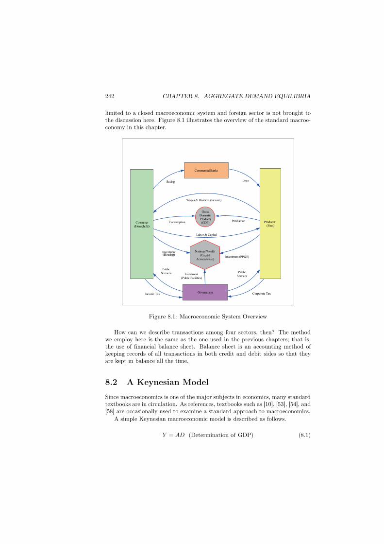
limited to a closed macroeconomic system and foreign sector is not brought tothe discussion here. Figure 8.1 illustrates the overview of the standard macroe-conomy in this chapter.
Consumer(Household)
Producer (Firm)
Commercial Banks
Government
National Wealth(Capital
Accumulation)
GrossDomesticProducts(GDP)
Labor & Capital
Wages & Dividens (Income)
Saving Loan
Investment (PP&E)
Investment(Housing)
Investment(Public Facilities)
Income Tax Corporate Tax
Consumption
PublicServices
PublicServices
Production
Figure 8.1: Macroeconomic System Overview
How can we describe transactions among four sectors, then? The methodwe employ here is the same as the one used in the previous chapters; that is,the use of financial balance sheet. Balance sheet is an accounting method ofkeeping records of all transactions in both credit and debit sides so that theyare kept in balance all the time.
8.2 A Keynesian Model
Since macroeconomics is one of the major subjects in economics, many standardtextbooks are in circulation. As references, textbooks such as [10], [53], [54], and[58] are occasionally used to examine a standard approach to macroeconomics.
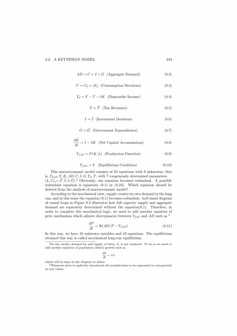
A simple Keynesian macroeconomic model is described as follows.
Y = AD (Determination of GDP) (8.1)
8.2. A KEYNESIAN MODEL 243
AD = C + I +G (Aggregate Demand) (8.2)
C = C0 + cYd (Consumption Decisions) (8.3)
Yd = Y − T − δK (Disposable Income) (8.4)
T = T (Tax Revenues) (8.5)
I = I (Investment Decisions) (8.6)
G = G (Government Expenditures) (8.7)
dK
dt= I − δK (Net Capital Accumulation) (8.8)
Yfull = F (K,L) (Production Function) (8.9)
Yfull = Y (Equilibrium Condition) (8.10)
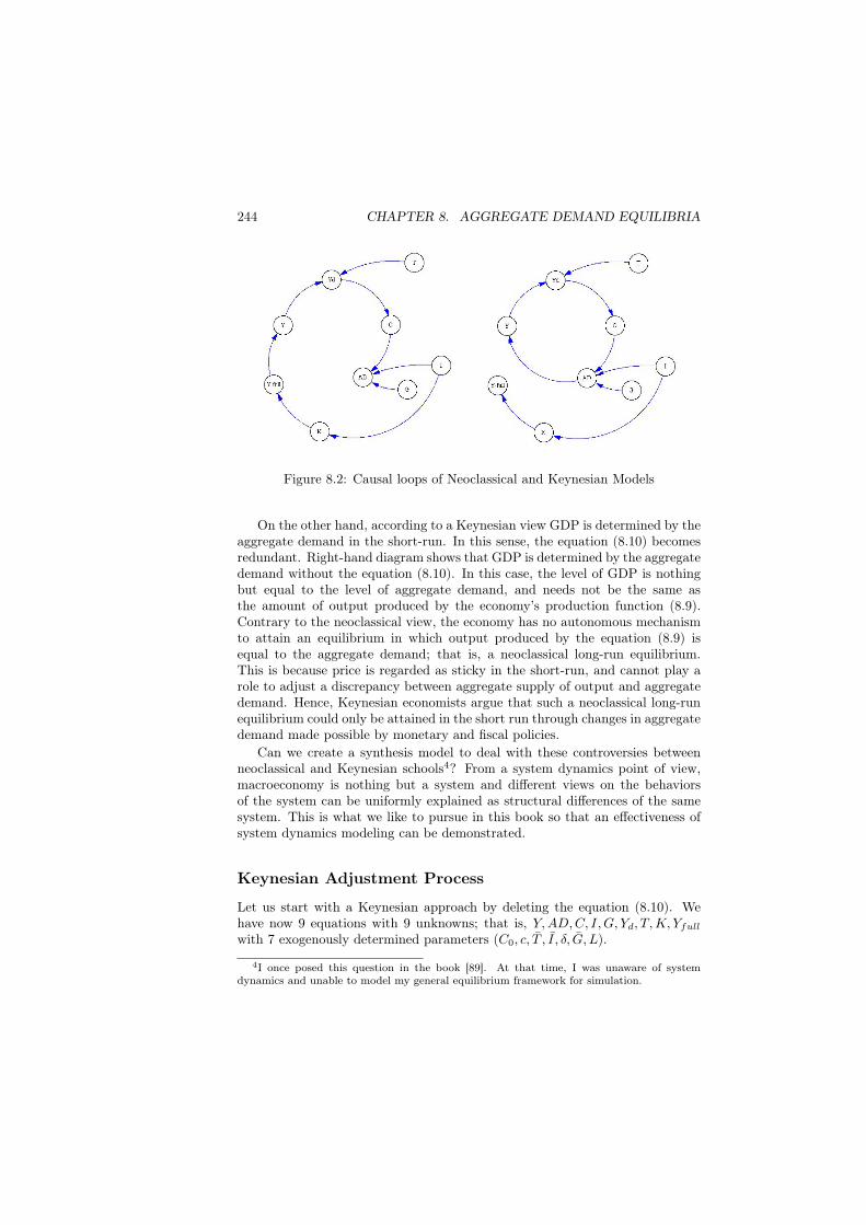
This macroeconomic model consists of 10 equations with 9 unknowns; thatis, Yfull, Y,K,AD,C, I,G, Yd, T , with 7 exogenously determined parameters(L,C0, c, T , I, δ, G).2 Obviously, one equation becomes redundant. A possibleredundant equation is equations (8.1) or (8.10). Which equation should bedeleted from the analysis of macroeconomic model?
According to the neoclassical view, supply creates its own demand in the longrun, and in this sense the equation (8.1) becomes redundant. Left-hand diagramof causal loops in Figure 8.2 illustrates how full capacity supply and aggregatedemand are separately determined without the equation(8.1). Therefore, inorder to complete this neoclassical logic, we need to add another equation ofprice mechanism which adjusts discrepancies between Yfull and AD such as 3
dP
dt= Ψ(AD/P − Yfull). (8.11)
In this way, we have 10 unknown variables and 10 equations. The equilibriumattained this way is called neoclassical long-run equilibrium.
2In this model, demand for and supply of labor, L, is not analyzed. To do so we need toadd another equation of population (labor) growth such as
dL
dt= nL
which will be done in the chapters to follow.3Whenever price is explicitly introduced, all variables have to be expressed (or interpreted)
as real values.
244 CHAPTER 8. AGGREGATE DEMAND EQUILIBRIA
Figure 8.2: Causal loops of Neoclassical and Keynesian Models
On the other hand, according to a Keynesian view GDP is determined by theaggregate demand in the short-run. In this sense, the equation (8.10) becomesredundant. Right-hand diagram shows that GDP is determined by the aggregatedemand without the equation (8.10). In this case, the level of GDP is nothingbut equal to the level of aggregate demand, and needs not be the same asthe amount of output produced by the economy’s production function (8.9).Contrary to the neoclassical view, the economy has no autonomous mechanismto attain an equilibrium in which output produced by the equation (8.9) isequal to the aggregate demand; that is, a neoclassical long-run equilibrium.This is because price is regarded as sticky in the short-run, and cannot play arole to adjust a discrepancy between aggregate supply of output and aggregatedemand. Hence, Keynesian economists argue that such a neoclassical long-runequilibrium could only be attained in the short run through changes in aggregatedemand made possible by monetary and fiscal policies.
Can we create a synthesis model to deal with these controversies betweenneoclassical and Keynesian schools4? From a system dynamics point of view,macroeconomy is nothing but a system and different views on the behaviorsof the system can be uniformly explained as structural differences of the samesystem. This is what we like to pursue in this book so that an effectiveness ofsystem dynamics modeling can be demonstrated.
Keynesian Adjustment Process
Let us start with a Keynesian approach by deleting the equation (8.10). Wehave now 9 equations with 9 unknowns; that is, Y,AD,C, I,G, Yd, T,K, Yfull
with 7 exogenously determined parameters (C0, c, T , I, δ, G, L).
4I once posed this question in the book [89]. At that time, I was unaware of systemdynamics and unable to model my general equilibrium framework for simulation.
8.2. A KEYNESIAN MODEL 245
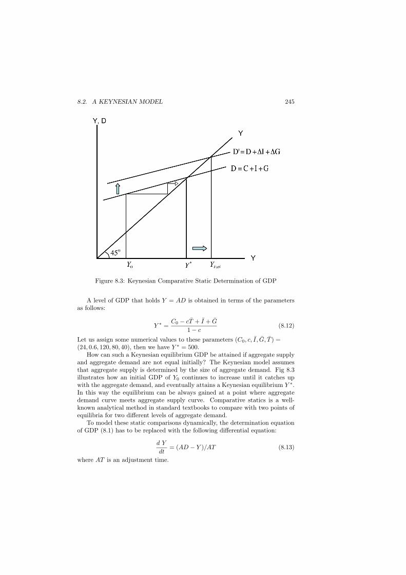
Figure 8.3: Keynesian Comparative Static Determination of GDP
A level of GDP that holds Y = AD is obtained in terms of the parametersas follows:
Y ∗ =C0 − cT + I + G
1− c(8.12)
Let us assign some numerical values to these parameters (C0, c, I, G, T ) =(24, 0.6, 120, 80, 40), then we have Y ∗ = 500.
How can such a Keynesian equilibrium GDP be attained if aggregate supplyand aggregate demand are not equal initially? The Keynesian model assumesthat aggregate supply is determined by the size of aggregate demand. Fig 8.3illustrates how an initial GDP of Y0 continues to increase until it catches upwith the aggregate demand, and eventually attains a Keynesian equilibrium Y ∗.In this way the equilibrium can be always gained at a point where aggregatedemand curve meets aggregate supply curve. Comparative statics is a well-known analytical method in standard textbooks to compare with two points ofequilibria for two different levels of aggregate demand.
To model these static comparisons dynamically, the determination equationof GDP (8.1) has to be replaced with the following differential equation:
d Y
dt= (AD − Y )/AT (8.13)
where AT is an adjustment time.
246 CHAPTER 8. AGGREGATE DEMAND EQUILIBRIA
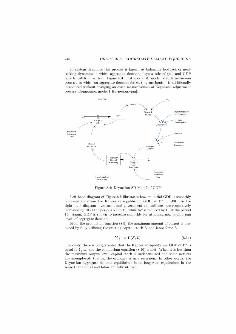
In system dynamics this process is known as balancing feedback or goal-seeking dynamics in which aggregate demand plays a role of goal and GDPtries to catch up with it. Figure 8.4 illustrates a SD model of such Keynesianprocess, in which an aggregate demand forecasting mechanism is additionallyintroduced without changing an essential mechanism of Keynesian adjustmentprocess [Companion model:1 Keynesian.vpm].
GDP
Change inGDP
Income
Consumption
Marginal Propensityto Consumer
+
+
+
AggregateDemand
Investment
GovernmentExpenditure
AggregateDemand
Forecasting Change inAD
Forecasting
ForecastingAdjustment
Time
++
+
DesiredProduction
+
+
+
ProductionAdjustment
Time
+
++
+
Initial GDP
DisposableIncome
Tax
+
+Basic
Consumption+
Error of Initial ADForecasting
Figure 8.4: Keynesian SD Model of GDP
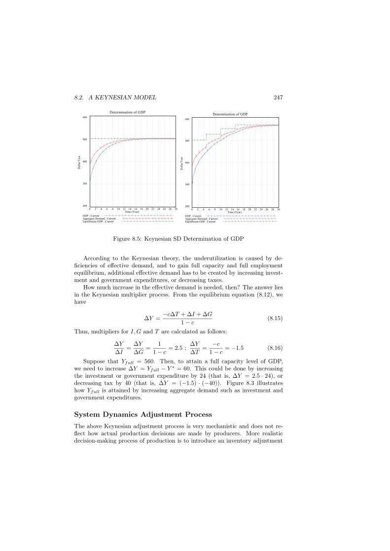
Left-hand diagram of Figure 8.5 illustrates how an initial GDP is smoothlyincreased to attain the Keynesian equilibrium GDP at Y ∗ = 500. In theright-hand diagram investment and government expenditures are respectivelyincreased by 10 at the periods 5 and 10, while tax is reduced by 10 at the period15. Again, GDP is shown to increase smoothly for attaining new equilibriumlevels of aggregate demand.
From the production function (8.9) the maximum amount of output is pro-duced by fully utilizing the existing capital stock K and labor force L.
Yfull = Y (K,L) (8.14)
Obviously, there is no guarantee that the Keynesian equilibrium GDP of Y ∗ isequal to Yfull, and the equilibrium equation (8.10) is met. When it is less thanthe maximum output level, capital stock is under-utilized and some workersare unemployed; that is, the economy is in a recession. In other words, theKeynesian aggregate demand equilibrium is no longer an equilibrium in thesense that capital and labor are fully utilized.
8.2. A KEYNESIAN MODEL 247
Determination of GDP
600
500
400
300
200
3 3 3 3 3 3 3 3 3 3 3 3 3 3 3 3 3 3 3 3 3 3 3 3 3 3 3
2
2
2
22
22
2 2 2 2 2 2 2 2 2 2 2 2 2 2 2 2 2 2 2 2
1
1
1
1
1
11
11
1 1 1 1 1 1 1 1 1 1 1 1 1 1 1 1 1 1
0 2 4 6 8 10 12 14 16 18 20 22 24 26 28 30Time (Year)
Doll
ar/Y
ear
GDP : Current 1 1 1 1 1 1 1 1 1 1 1 1 1 1 1 1 1 1 1 1 1
Aggregate Demand : Current 2 2 2 2 2 2 2 2 2 2 2 2 2 2 2 2
Equilibrium GDP : Current 3 3 3 3 3 3 3 3 3 3 3 3 3 3 3 3
Determination of GDP
600
500
400
300
200
3 3 3 3
3 3 3 3 3
3 3 3 3 3
3 3 3 3 3 3 3 3 3 3 3 3 3
2
2
2
22
22
22
22
2 2 22 2 2 2 2 2 2 2 2 2 2 2 2 2
1
1
1
1
1
1
1
11
11
11
11
11
1 1 1 1 1 1 1 1 1 1 1
0 2 4 6 8 10 12 14 16 18 20 22 24 26 28 30Time (Year)
Do
llar
/Yea
r
GDP : Current 1 1 1 1 1 1 1 1 1 1 1 1 1 1 1 1 1 1 1 1 1 1
Aggregate Demand : Current 2 2 2 2 2 2 2 2 2 2 2 2 2 2 2 2 2
Equilibrium GDP : Current 3 3 3 3 3 3 3 3 3 3 3 3 3 3 3 3 3
Figure 8.5: Keynesian SD Determination of GDP
According to the Keynesian theory, the underutilization is caused by de-ficiencies of effective demand, and to gain full capacity and full employmentequilibrium, additional effective demand has to be created by increasing invest-ment and government expenditures, or decreasing taxes.
How much increase in the effective demand is needed, then? The answer liesin the Keynesian multiplier process. From the equilibrium equation (8.12), wehave
∆Y =−c∆T +∆I +∆G
1− c(8.15)
Thus, multipliers for I,G and T are calculated as follows:
∆Y
∆I=
∆Y
∆G=
1
1− c= 2.5 ;
∆Y
∆T=
−c
1− c= −1.5 (8.16)
Suppose that Yfull = 560. Then, to attain a full capacity level of GDP,we need to increase ∆Y = Yfull − Y ∗ = 60. This could be done by increasingthe investment or government expenditure by 24 (that is, ∆Y = 2.5 · 24), ordecreasing tax by 40 (that is, ∆Y = (−1.5) · (−40)). Figure 8.3 illustrateshow Yfull is attained by increasing aggregate demand such as investment andgovernment expenditures.
System Dynamics Adjustment ProcessThe above Keynesian adjustment process is very mechanistic and does not re-flect how actual production decisions are made by producers. More realisticdecision-making process of production is to introduce an inventory adjustment
248 CHAPTER 8. AGGREGATE DEMAND EQUILIBRIA
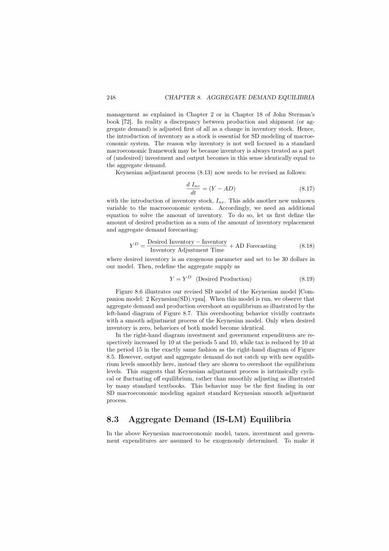
management as explained in Chapter 2 or in Chapter 18 of John Sterman’sbook [72]. In reality a discrepancy between production and shipment (or ag-gregate demand) is adjusted first of all as a change in inventory stock. Hence,the introduction of inventory as a stock is essential for SD modeling of macroe-conomic system. The reason why inventory is not well focused in a standardmacroeconomic framework may be because inventory is always treated as a partof (undesired) investment and output becomes in this sense identically equal tothe aggregate demand.
Keynesian adjustment process (8.13) now needs to be revised as follows:
d Invdt
= (Y −AD) (8.17)
with the introduction of inventory stock, Inv. This adds another new unknownvariable to the macroeconomic system. Accordingly, we need an additionalequation to solve the amount of inventory. To do so, let us first define theamount of desired production as a sum of the amount of inventory replacementand aggregate demand forecasting:
Y D =Desired Inventory − Inventory
Inventory Adjustment Time+ AD Forecasting (8.18)
where desired inventory is an exogenous parameter and set to be 30 dollars inour model. Then, redefine the aggregate supply as
Y = Y D (Desired Production) (8.19)
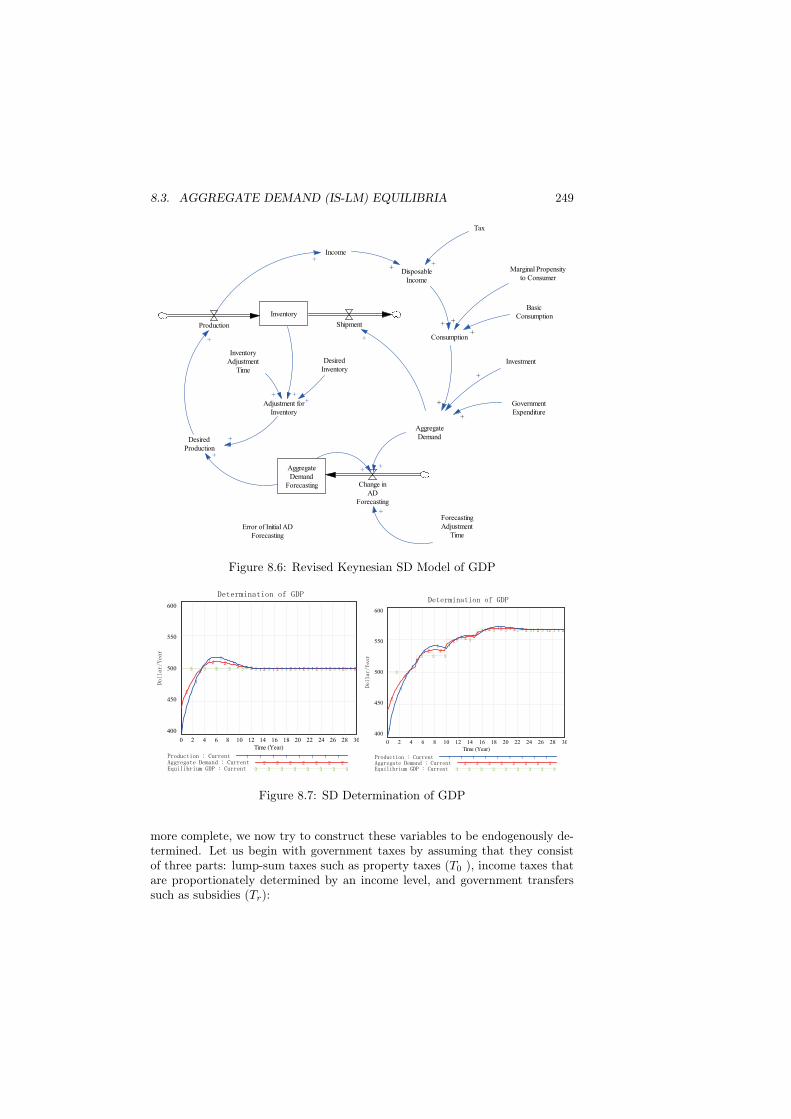
Figure 8.6 illustrates our revised SD model of the Keynesian model [Com-panion model: 2 Keynesian(SD).vpm]. When this model is run, we observe thataggregate demand and production overshoot an equilibrium as illustrated by theleft-hand diagram of Figure 8.7. This overshooting behavior vividly contrastswith a smooth adjustment process of the Keynesian model. Only when desiredinventory is zero, behaviors of both model become identical.
In the right-hand diagram investment and government expenditures are re-spectively increased by 10 at the periods 5 and 10, while tax is reduced by 10 atthe period 15 in the exactly same fashion as the right-hand diagram of Figure8.5. However, output and aggregate demand do not catch up with new equilib-rium levels smoothly here, instead they are shown to overshoot the equilibriumlevels. This suggests that Keynesian adjustment process is intrinsically cycli-cal or fluctuating off equilibrium, rather than smoothly adjusting as illustratedby many standard textbooks. This behavior may be the first finding in ourSD macroeconomic modeling against standard Keynesian smooth adjustmentprocess.
8.3 Aggregate Demand (IS-LM) EquilibriaIn the above Keynesian macroeconomic model, taxes, investment and govern-ment expenditures are assumed to be exogenously determined. To make it
8.3. AGGREGATE DEMAND (IS-LM) EQUILIBRIA 249
Income
Consumption
Marginal Propensityto Consumer
+
+
AggregateDemand
Investment
GovernmentExpenditure
AggregateDemand
Forecasting Change inAD
Forecasting
ForecastingAdjustment
Time
++
+
DesiredProduction
+
+
+
+
Inventory
Production Shipment
+
DesiredInventory
Adjustment forInventory
InventoryAdjustment
Time
++
+
+
+
+
Error of Initial ADForecasting
BasicConsumption
+
Tax
DisposableIncome
+
+
Figure 8.6: Revised Keynesian SD Model of GDP
'HWHUPLQDWLRQ�RI�*'3600
550
500
450
400
3 3 3 3 3 3 3 3 3 3 3 3 3
2
2
2 22
2 2 2 2 2 2 2 2 2
1
1
11
11
1 1 1 1 1 1 1 1
0 2 4 6 8 10 12 14 16 18 20 22 24 26 28 30Time (Year)
'ROODU�<HDU
3URGXFWLRQ���&XUUHQW 1 1 1 1 1 1 1 1
$JJUHJDWH�'HPDQG���&XUUHQW 2 2 2 2 2 2 2
(TXLOLEULXP�*'3���&XUUHQW 3 3 3 3 3 3 3 3
'HWHUPLQDWLRQ�RI�*'3600
550
500
450
400
3 3
3 3 3
3 3
3 3 3 3 3 3 3
2
2
2
2 2
22
22 2 2 2 2 2 2
1
1
1
1
1 1
1 1
11 1 1 1 1 1
0 2 4 6 8 10 12 14 16 18 20 22 24 26 28 30Time (Year)
'ROODU�<HDU
3URGXFWLRQ���&XUUHQW 1 1 1 1 1 1 1 1 1
$JJUHJDWH�'HPDQG���&XUUHQW 2 2 2 2 2 2 2 2
(TXLOLEULXP�*'3���&XUUHQW 3 3 3 3 3 3 3 3 3
Figure 8.7: SD Determination of GDP
more complete, we now try to construct these variables to be endogenously de-termined. Let us begin with government taxes by assuming that they consistof three parts: lump-sum taxes such as property taxes (T0 ), income taxes thatare proportionately determined by an income level, and government transferssuch as subsidies (Tr):
250 CHAPTER 8. AGGREGATE DEMAND EQUILIBRIA
T = T0 + tY − Tr (8.20)
where t is an income tax rate.Next, investment is assumed to be determined by the interest rate:
I(i) =I0i− αi (8.21)
where α is an interest sensitivity of investment. We have now added a newunknown variable of the interest rate to the model, and hence an additionalequation is needed to make it complete. According to the standard textbook,it should be an equilibrium condition in money market such that real moneysupply used in a year is equal to the demand for money:
Ms
PV = aY − bi (8.22)
where V is velocity of money having a unit 1/year, a is a fraction of income fortransactional demand for money, and b is an interest sensitivity of demand formoney. P is a price level and it is treated as a sticky exogenous parameter.
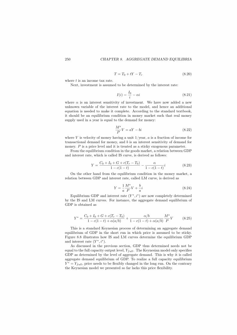
From the equilibrium condition in the goods market, a relation between GDPand interest rate, which is called IS curve, is derived as follows:
Y =C0 + I0 +G+ c(Tr − T0)
1− c(1− t)− α
1− c(1− t)i (8.23)
On the other hand from the equilibrium condition in the money market, arelation between GDP and interest rate, called LM curve, is derived as
Y =1
a
Ms
PV +
b
ai (8.24)
Equilibrium GDP and interest rate (Y ∗, i∗) are now completely determinedby the IS and LM curves. For instance, the aggregate demand equilibrium ofGDP is obtained as
Y ∗ =C0 + I0 +G+ c(Tr − T0)
1− c(1− t) + α(a/b)+
α/b
1− c(1− t) + α(a/b)
Ms
PV (8.25)
This is a standard Keynesian process of determining an aggregate demandequilibrium of GDP in the short run in which price is assumed to be sticky.Figure 8.8 illustrates how IS and LM curves determine the equilibrium GDPand interest rate (Y ∗, i∗).
As discussed in the previous section, GDP thus determined needs not beequal to the full capacity output level, Yfull. The Keynesian model only specifiesGDP as determined by the level of aggregate demand. This is why it is calledaggregate demand equilibrium of GDP. To realize a full capacity equilibriumY ∗ = Yfull, price needs to be flexibly changed in the long run. On the contrarythe Keynesian model we presented so far lacks this price flexibility.
8.3. AGGREGATE DEMAND (IS-LM) EQUILIBRIA 251
Co+ I
o+G + c(T
r−T
o)
1− c(1− t)
Co+ I
o+G + c(T
r−T0)
α䌉䌓 Curve
VP
M
a
s1
䌌䌍 Curve
Y
i
Y*
i*
Equilibrium
(Y *,i*)
Figure 8.8: IS-LM Determination of GDP and Interest Rate
Endogenous Government ExpendituresWe have successfully made variables such as T and I endogenous. The onlyremaining exogenous variable is government expenditures, G. They are usuallydetermined by a democratic political process, and in this sense could be leftoutside the system as an exogenously determined parameter.
Instead, we try to make it an endogenous variable. First approach is toassume that the government expenditures are dependent on the economic growthrate, g(t) = ∆Y (t)/Y (t), such that
d G
dt= g(t)G. (8.26)
This approach seems to be reasonable because many governments try toincrease government expenditures proportionally to their economic growth ratesso that a run-away accumulation of government deficit will be avoided.
Second approach is to assume that government expenditures are dependenton its tax revenues, since the main source of government expenditures is taxrevenues which are endogenously determined by the size of output or incomelevel. Then government expenditures become a function of tax revenues:
G = βT (8.27)
252 CHAPTER 8. AGGREGATE DEMAND EQUILIBRIA
where β is a ratio between government expenditures and tax revenues, calledprimary balance ratio here. When β = 1, we have a so-called balanced budget,while if β > 1, we have budget deficit.
With the introduction of the government expenditures in either one of thesetwo ways, all exogenously determined variables such as T, I, and G are nowendogenously determined within the macroeconomic system.
Let us analyze the second case furthermore. In this case IS curve becomes
Y =C0 + I0 + (β − c)(T0 − Tr)
1− c− (β − c)t− α
1− c− (β − c)ti (8.28)
By rearranging, the aggregate demand equilibrium of GDP is calculated as
Y ∗ =C0 + I0 + (β − c)(T0 − Tr)
1− c− (β − c)t+ α(a/b)+
α/b
1− c− (β − c)t+ α(a/b)
Ms
PV (8.29)
How does the introduction of tax-dependent expenditures affect behaviorsof the equilibrium? Let us consider, as one special case, how a tax reduction inlump-sum taxes, T0, affect the equilibrium GDP under a balanced budget; thatis, β = 1. In this case, we have from the equation (8.29)
dY
dT0=
1− c
(1− c)(1− t) + α(a/b)> 0 (8.30)
On the other hand, in the case of the exogenously determined expenditures,we have from the equation (8.25)
dY
dT0=
−c
1− c(1− t) + α(a/b)< 0 (8.31)
This implies that under a balanced budget a reduction in lump-sum taxeswill discourage GDP, contrary to a general belief that it stimulates the economy.This counter-intuitive feature seems to be deemphasized in standard textbooksin which tax cut is usually treated as stimulating the economy.
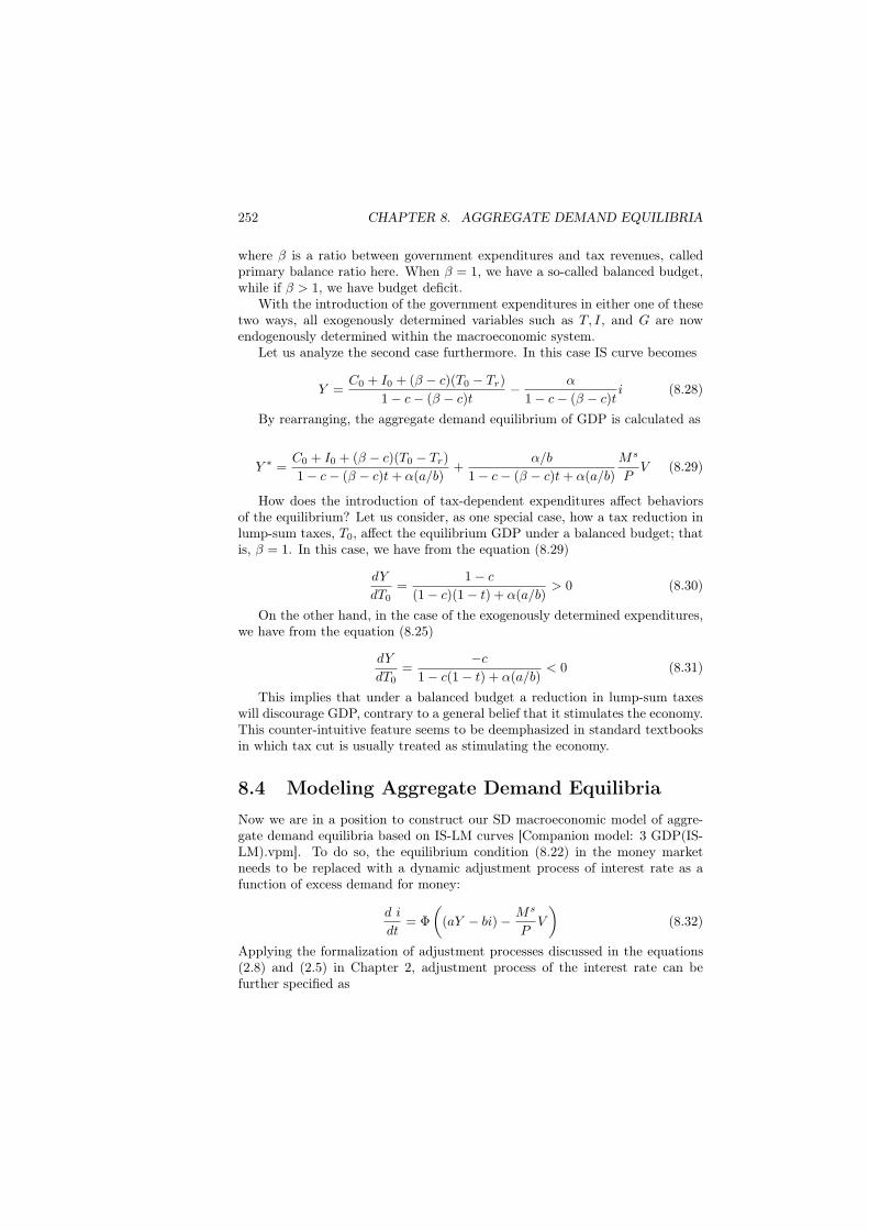
8.4 Modeling Aggregate Demand EquilibriaNow we are in a position to construct our SD macroeconomic model of aggre-gate demand equilibria based on IS-LM curves [Companion model: 3 GDP(IS-LM).vpm]. To do so, the equilibrium condition (8.22) in the money marketneeds to be replaced with a dynamic adjustment process of interest rate as afunction of excess demand for money:
d i
dt= Φ
((aY − bi)− Ms
PV
)(8.32)
Applying the formalization of adjustment processes discussed in the equations(2.8) and (2.5) in Chapter 2, adjustment process of the interest rate can befurther specified as
8.4. MODELING AGGREGATE DEMAND EQUILIBRIA 253
d i
dt=
i∗ − i
DelayTime(8.33)
where the desired interest rate i∗ is obtained as
i∗ =i(
Ms
P V/(aY − bi))e , (8.34)
in which e denotes a money ratio elasticity of desired interest rate.Figure 8.9 illustrates the adjustment process of interest rate.
Interest Rate
Change inInterest Rate
Demand forMoney
<AggregateDemand>
Interest Sensitivity ofMoney Demand
MoneySupply
Income Fractionfor Transaction
Delay Time of InterestRate Change
Initial MoneySupply
Change inMoney Supply
Time forMonetary Policy
Velocity ofMoney
Supply ofMoneyMoney
Supply(g)Change in Money
Supply(g)
<Growth Rate>
Swithch(Money)
MoneyRatio
Effect onInterest Rate
Ratio Elasticity (Effecton Interest Rate)
DesiredInterest Rate
InitialInterest Rate
Figure 8.9: Interest Rate Adjustment Process
With this replacement, we could directly build a SD macroeconomic modelof aggregate demand model in a mechanistic way such that IS and LM curvesinteract one another as developed in Figure 8.8 in the previous section. Thiscould be a better approach than the comparative static analysis in which IS andLM curves are manually sifted to observe how aggregate demand equilibrium of(Y ∗, i∗) is changed as usually done in the standard textbooks.
However, from a system dynamics point of view, this mechanistic approachof modeling aggregate demand equilibria may incur many causal loopholes. Forinstance, when consumers save, they receive interests from banks. If govern-ment spends more than receives, its deficit has to be funded by consumers asa purchase of government securities, against which they also receive interests.Whenever the macroeconomy is viewed as a wholistic economic system, thesetransactions play important feedback roles and such feedback effects need not beneglected. Therefore, as a complete system it should include those transactionsamong consumers, producers, banks and government from the beginning.
Due to the existence of these causal loopholes, standard macroeconomicframework has resulted in offering many open spaces which macroeconomists areinvited to fill in with their own ideas and theories. We believe these open spaceshave been intrinsic causes of many macroeconomic controversies such as the one
254 CHAPTER 8. AGGREGATE DEMAND EQUILIBRIA
between neoclassical and Keynesian schools of economics. These controversies,moreover, give us an impression that their macroeconomic models are mutuallyexclusive and cannot be integrated like oil and water.
On the contrary, as system dynamics researchers we believe that macro-economy as a system could be modeled as an integrated whole so that con-troversies such as described above are nothing but different behaviors causedby slightly different conditions of the same system structure. In this sense, itssystem dynamics model, if built completely, could synthesize these controver-sies as different macroeconomic system behaviors, rather than the behaviors ofdifferent economic system structures. This has been our main motivation forconstructing a wholistic SD macroeconomic model in this book.
For the construction of synthetic model, a double entry accounting systemof corporate balance sheet turns out to be very effective for describing manytransactions among macroeconomic sectors. To some reader this approach seemsto make our modeling unnecessarily complicated compared with the standardmacroeconomic framework. We pose, however, that this is the simplest way todescribe complicated macroeconomic behaviors per se.
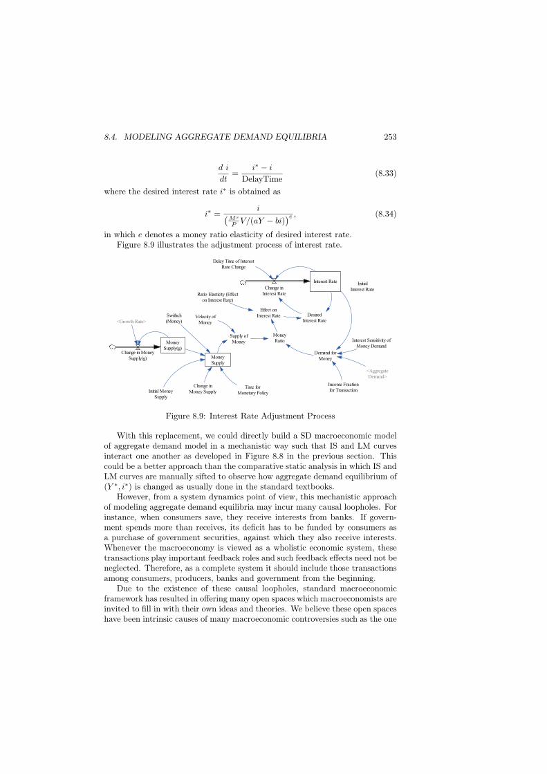
ProducersLet us now describe some fundamental transactions which are missing in thestandard textbook framework. We begin with producers. In the macroeconomicsystem, they face two important decisions: production for this year and invest-ment for the futures. We have already assumed that production decision is madeby the equation (8.19) by following a system dynamics approach of inventorymanagement, while investment decision is assumed to be made by a standardmacroeconomic investment function (8.21).
Based on these decisions, major transactions of producers are, as illustratedin Figure 8.10, summarized as follows.
• Producers are constantly in a state of cash flow deficits as analyzed inChapter 4. To make new investment, therefore, they have to borrow moneyfrom banks and pay interest to the banks.
• Out of the revenues producers deduct the amount of depreciation and paywages to workers (consumers) and interests to the banks. The remainingrevenues become profits before tax.
• They pay corporate tax to the government.
• The remaining profits are paid to the owners (that is, consumers) as div-idends.
ConsumersConsumers have to make two decisions: how much to consume and how muchto invest the remaining income between saving and government securities - a
8.4. MODELING AGGREGATE DEMAND EQUILIBRIA 255
Inve
ntor
y
Pro
duct
ion
Sal
es
<D
esir
ed P
rodu
ctio
n><
Agg
rega
te D
eman
d>
Cas
h (P
rodu
cer)
Ret
aine
dE
arni
ngs
(Pro
duce
r)
Rev
enue
s
<P
rodu
ctio
n>
Wag
es
Div
iden
ds
Pro
fits
befo
re T
ax
Dis
trib
utio
nR
atio
of
Wag
es
<W
ages
>
<W
ages
>
Cas
hF
low
<D
ivid
ends
>
Cap
ital
(PP
& E
)
Cap
ital
Sto
ck
Dep
reci
atio
n
Dep
reci
atio
nR
ate
<In
vest
men
t>C
apita
l S
tock
New
ly I
ssue
d
<S
ales
>
Deb
t(P
rodu
cer)
Bor
row
ing
<B
orro
win
g>
<B
orro
win
g>
<D
epre
ciat
ion>
Cas
h F
low
fro
mO
pera
ting
Act
iviti
es
Cas
h F
low
fro
mIn
vest
ing
Act
iviti
es
Cas
h F
low
Def
icit
<In
vest
men
t>
New
Cap
ital
Sto
ck
Bor
row
ing
Rat
io
<N
ew C
apita
l S
tock
>
Cas
h F
low
fro
mF
inan
cing
Act
iviti
es
<N
ew C
apita
lS
tock
>
Ope
ratin
gA
ctiv
ities
Inve
stin
gA
ctiv
ities
Fin
anci
ngA
ctiv
ities
<D
ivid
ends
>
Fun
d-R
aisi
ngA
mou
ntC
orpo
rate
Tax
Rat
e
Pro
fits
Cor
pora
teT
ax
<C
orpo
rate
Tax
>
<C
orpo
rate
Tax
>
<In
tere
st p
aid
by P
rodu
cer>
<In
tere
st p
aid
by P
rodu
cer>
<In
tere
st p
aid
by P
rodu
cer>
<In
tere
st p
aid
byP
rodu
cer>
<F
ull
Pro
duct
ion>
Tax
on
Pro
duct
ion
Exc
ise
Tax
Rat
e
<T
ax o
nP
rodu
ctio
n>
<T
ax o
nP
rodu
ctio
n>
Cha
nge
in E
xcic
eT
ax R
ate
<T
ime
for
Fis
cal
Pol
icy>
Pay
men
t by
Pro
duce
r
<P
aym
ent b
yP
rodu
cer>
Figure 8.10: Transactions of Producers
256 CHAPTER 8. AGGREGATE DEMAND EQUILIBRIA
Cas
h(C
onsu
mer
)
Consu
mpti
on
Bas
icC
onsu
mpti
on
Mar
gin
alP
ropen
sity
to
Consu
mer
Dep
osi
ts(C
onsu
mer
)
Sav
ing
Shar
es(C
onsu
mer
)
<C
apit
al S
tock
New
ly I
ssued
>
Fin
anci
alIn
ves
tmen
t(S
har
es)
Inco
me
Tax
Inco
me
Tax
Rat
e
Dis
posa
ble
Inco
me
Gover
nm
ent
Sec
uri
ties
(Consu
mer
)
Fin
anci
al I
nves
tmen
t(S
ecuri
ties
)
<G
over
nm
ent
Sec
uri
ties
>
Inco
me
Dis
trib
uti
on
by
Pro
duce
rs
<D
epre
ciat
ion>
<C
orp
ora
te T
ax>
<W
ages
>
<D
ivid
ends>
<In
tere
st p
aid b
yP
roduce
r>
Dis
trib
ute
d I
nco
me
Lum
p-s
um
Tax
es
Gover
nm
ent
Tra
nsf
ers
Chan
ge
in L
um
p-s
um
Tax
es
Consu
mer
Equit
y
Inco
me
<W
ages
>
<In
tere
st p
aid b
yB
anks>
<D
ivid
ends>
<In
tere
st p
aid b
y th
eG
over
nm
ent>
<In
com
e>
<D
isposa
ble
Inco
me>
Sec
uri
ties
sold
by
Consu
mer
s <G
over
nm
ent
De
bt
Red
empti
on>
Chan
ge
in I
nco
me
Tax
Rat
e
<T
ime
for
Fis
cal
Poli
cy>
<E
xci
se T
ax R
ate>
Init
ial
Dep
osi
ts(C
onsu
mer
)
Init
ial
Shar
es(C
onsu
mer
)
<In
com
e>
Figure 8.11: Transactions of Consumer
8.4. MODELING AGGREGATE DEMAND EQUILIBRIA 257
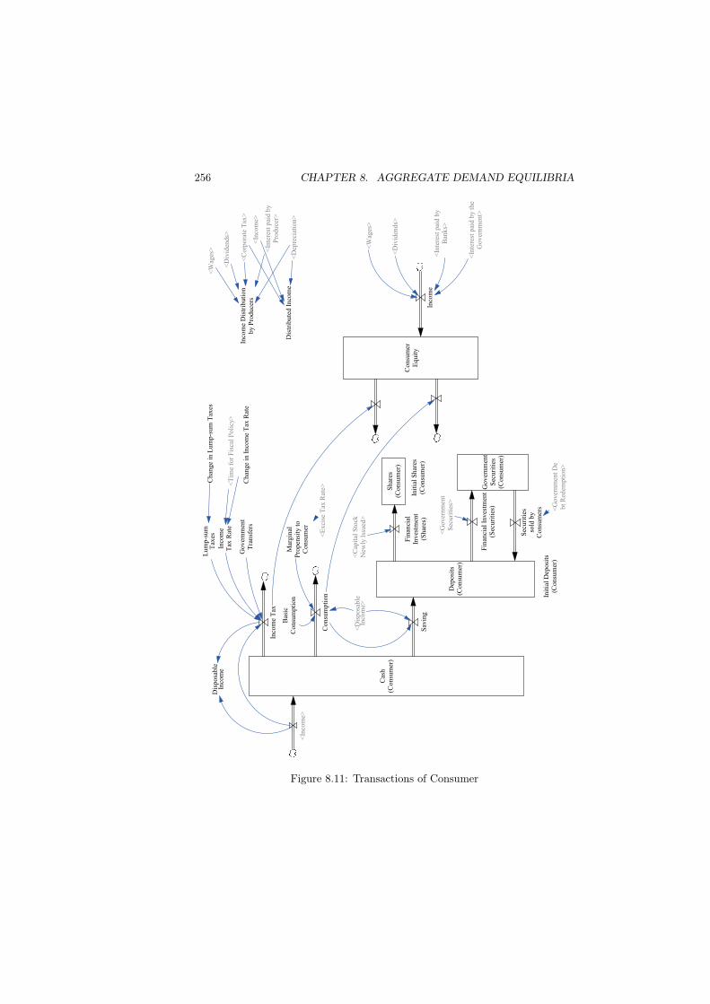
portfolio choice. Consumption decision is assumed to be made by a standardconsumption function (8.3). (It could also be made dependent on their financialassets). As to the portfolio decision we simply assume that consumers first savethe remaining income as deposits, out of which, then, they purchase governmentsecurities.
Transactions of consumers are illustrated in Figure 8.11, some of which aresummarized as follows.
• Consumers receive wages and dividends.
• In addition, they receive interest from banks and the government that isderived from their financial assets consisting of bank deposits and govern-ment securities.
• Financial investment of government securities is made out of the accountof deposits. (In this model, no corporate shares are assumed to be pur-chased).
• Out of the cash income as a whole, consumers pay income taxes, and theremaining amount becomes their disposal income.
• Out of their disposal income, they spend on consumption. The remainingamount is saved. Accordingly, no cash is assumed to be withheld by theconsumers.
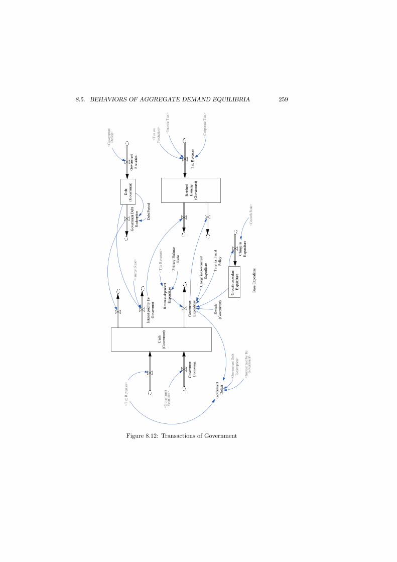
GovernmentGovernment faces decisions such as how much taxes to levy as revenues andhow much to spend as expenditures. Tax revenues are assumed to be collectedaccording to the standard formula in (8.20), while expenditures are determinedeither by growth-dependent amount (8.26) or revenue-dependent amount (8.27).In the model, expenditures are easily switched to either one. Revenue-dependentexpenditure is set as default.
Transactions of the government are illustrated in Figure 8.12, some of whichare summarized as follows.
• Government receives, as tax revenues, income taxes from consumers andcorporate taxes from producers. It also levies excise tax on production.
• Government spending consists of government expenditures and paymentsto the consumers such as debt redemption and interests against its secu-rities.
• Government expenditures are assumed to be endogenously determinedby either the growth-dependent expenditures or tax revenue-dependentexpenditures.
• If spending exceeds tax revenues, government has to borrow cash fromconsumers by newly issuing government securities.
258 CHAPTER 8. AGGREGATE DEMAND EQUILIBRIA
Banks
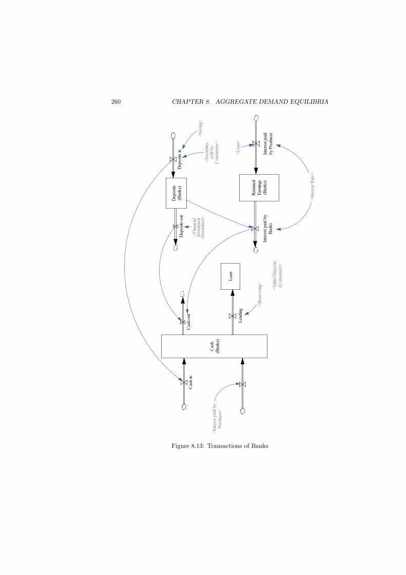
In our model, banks are assumed to play a very passive role; that is, theyonly make loans to producers by the amount asked by them. In other words,they don’t purchase government securities and accordingly need to make noportfolio decisions between loans and securities. This assumption is droppedin the following chapters. Transactions of banks are illustrated in Figure 8.13,some of which are summarized as follows.
• Banks receive deposits from consumers, against which they pay interests.
• They make loans to producers and receive interests. Prime interest ratefor loans is assumed to be the same as the interest rate for deposits. Thisassumption is dropped in the following chapters.
• Their retained earnings thus become interest receipts from producers lessinterest payment to consumers.
8.5 Behaviors of Aggregate Demand Equilibria
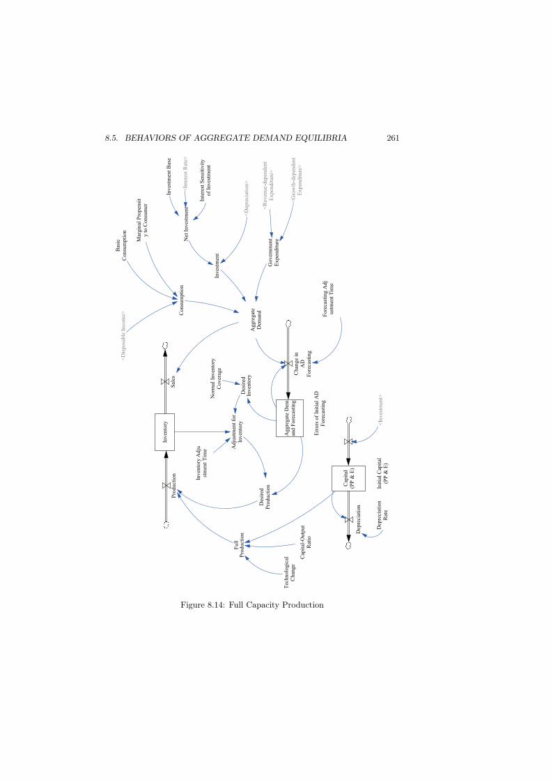
We now see how aggregate demand equilibrium of (Y ∗, i∗) is attained in ourSD model constructed above. This model is built by deleting the equation(8.10) and in this sense, as already discussed above, Y ∗ needs not be equal toa production level of full capacity, Yfull. Surely, the full production level is amaximum level of output in the economy beyond which no physical output ispossible. To introduce this upper bound of production level, the equation (8.19)has to be revised as follows.
Y = Min(Yfull, Y D) (8.35)
Moreover, the full capacity output level in equation (8.14) is specified as follows:
Yfull = eκt1
θK (8.36)
where κ is an annual increase rate of technological progress, and θ is a capital-output ratio. For simplicity, labor force is not considered here. The productionprocess of GDP in our SD model is illustrated in Figure 8.14.
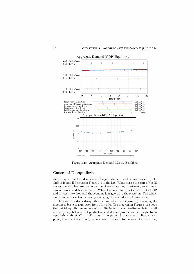
Top diagram in Figure 8.15 shows mostly equilibrium growth path of pro-duction around full capacity level. Bottom diagram is loci of aggregate demandequilibrium (Y ∗, i∗) such as an intersection between IS-LM curves as illustratedin Figure 8.8. Our model can capture these dynamic movements of the aggre-gate demand equilibria in contrast with comparative static ones in standardtextbooks. This may be another contribution of SD macroeconomic modeling.
8.5. BEHAVIORS OF AGGREGATE DEMAND EQUILIBRIA 259
Cas
h(G
over
nmen
t)
Deb
t(G
over
nmen
t)
Gov
ernm
ent
Exp
endi
ture
Gov
ernm
ent
Def
icit
Gov
ernm
ent
Sec
uriti
es
Gov
ernm
ent
Bor
row
ing
Inte
rest
pai
d by
the
Gov
ernm
ent
Cha
nge
in G
over
nmen
tE
xpen
ditu
re
Tim
e fo
r F
isca
lP
olic
y
Pri
mar
y B
alan
ceR
atio
Bas
e E
xpen
ditu
re
Rev
enue
-dep
ende
ntE
xpen
ditu
re
Gov
ernm
ent D
ebt
Red
empt
ion
Deb
t Per
iod
Ret
aine
dE
arni
ngs
(Gov
ernm
ent)
Tax
Rev
enue
s
<In
com
e T
ax>
<C
orpo
rate
Tax
>
<G
over
nmen
tS
ecur
ities
>
<T
ax R
even
ues>
<T
ax R
even
ues>
<In
tere
st p
aid
by th
eG
over
nmen
t>
<G
over
nmen
tD
efic
it>
<G
over
nmen
t Deb
tR
edem
ptio
n>
<G
row
th R
ate>
Gro
wth
-dep
ende
ntE
xpen
ditu
reC
hang
e in
Exp
endi
ture
<T
ax o
nP
rodu
ctio
n>
<In
tere
st R
ate>
Sw
itch
(Gov
ernm
ent)
Figure 8.12: Transactions of Government
260 CHAPTER 8. AGGREGATE DEMAND EQUILIBRIA
Dep
osi
ts(B
ank
s)
Cas
h(B
ank
s)
Lo
an
Dep
osi
ts in
Cas
h in
Len
din
g
<S
avin
g>
<B
orr
ow
ing>
Ret
aine
dE
arni
ngs
(Ban
ks)
Inte
rest
pai
d b
yB
ank
s
<In
tere
st R
ate>
Inte
rest
pai
db
y P
rod
ucer
<In
tere
st p
aid
by
Pro
duc
er>
<In
itial
Dep
osi
ts(C
ons
umer
)>
Dep
osi
ts o
ut
Cas
h o
ut
<F
inan
cial
Inve
stm
ent
(Sec
uriti
es)>
<S
ecur
ities
sold
by
Co
nsum
ers>
<L
oan
>
Figure 8.13: Transactions of Banks
8.5. BEHAVIORS OF AGGREGATE DEMAND EQUILIBRIA 261M
argin
al P
rop
ensi
ty
to C
on
sum
er
Aggre
gat
eD
eman
d
Net
In
ves
tmen
t
Aggre
gat
e D
eman
d F
ore
cast
ing
Ch
ange
inA
DF
ore
cast
ing
Fo
reca
stin
g A
dj
ust
men
t T
ime
Des
ired
Pro
du
ctio
n
Inv
ento
ry
Pro
du
ctio
nS
ales
Des
ired
Inv
ento
ry
Ad
just
men
t fo
rIn
ven
tory
Inv
ento
ry A
dju
stm
ent
Tim
e
Err
ors
of
Init
ial
AD
Fo
reca
stin
g
Bas
icC
on
sum
pti
on
Inv
estm
ent
<D
epre
ciat
ion
>
Co
nsu
mp
tio
n
Inv
estm
ent
Bas
e
Inte
rest
Sen
siti
vit
yo
f In
ves
tmen
t
<D
isp
osa
ble
In
com
e>
Go
ver
nm
ent
Ex
pen
dit
ure
Cap
ital
(PP
& E
)D
epre
ciat
ion
Dep
reci
atio
nR
ate
<In
ves
tmen
t>
Cap
ital
-Ou
tpu
tR
atio
Fu
llP
rod
uct
ion
No
rmal
In
ven
tory
Co
ver
age
<R
even
ue-
dep
end
ent
Ex
pen
dit
ure
>
<In
tere
st R
ate>
<G
row
th-d
epen
den
tE
xp
end
itu
re>
Init
ial
Cap
ital
(PP
& E
)
Tec
hn
olo
gic
alC
han
ge
Figure 8.14: Full Capacity Production
262 CHAPTER 8. AGGREGATE DEMAND EQUILIBRIA
Aggregate Demand (GDP) Equilibria
600 Dollar/Year0.06 1/Year
300 Dollar/Year-0.26 1/Year
0 Dollar/Year-0.58 1/Year
6 6 6 6 6 6
5 5 5 5 5 5
4 4 4 4 4 4
3 3 3 3 3 3
2 2 2 2 2 2 21 1 1 1 1 1 1
0 5 10 15 20 25 30 35Time (Year)
Production : Equilibria Dollar/Year1 1 1Aggregate Demand : Equilibria Dollar/Year2 2 2Consumption : Equilibria Dollar/Year3 3 3 3Investment : Equilibria Dollar/Year4 4 4 4Full Production : Equilibria Dollar/Year5 5 5 5Growth Rate : Equilibria 1/Year6 6 6 6
Aggregate Demand (IS-LM) Equiilibria
2.4
2.05
1.7
1.35
1
1 1 1 1 1 1 1 1 1 1 1 1 11
409 411 413 415 417 419 421 423 425 427Production
Per
cent/
Yea
r
Interest Rate 1 1 1 1 1 1 1 1 1 1 1
Figure 8.15: Aggregate Demand Mostly Equilibria
Causes of Disequilibria
According to the IS-LM analysis, disequilibria or recessions are caused by theshift of IS and lM curves in Figure 7.8 to the left. What causes the shift of the IScurves, then? They are the deduction of consumption, investment, governmentexpenditures, and tax increases. When IS curve shifts to the left, both GDPand interest rate drop and the economy is triggered to the recession. The readercan examine these five causes by changing the related model parameters.
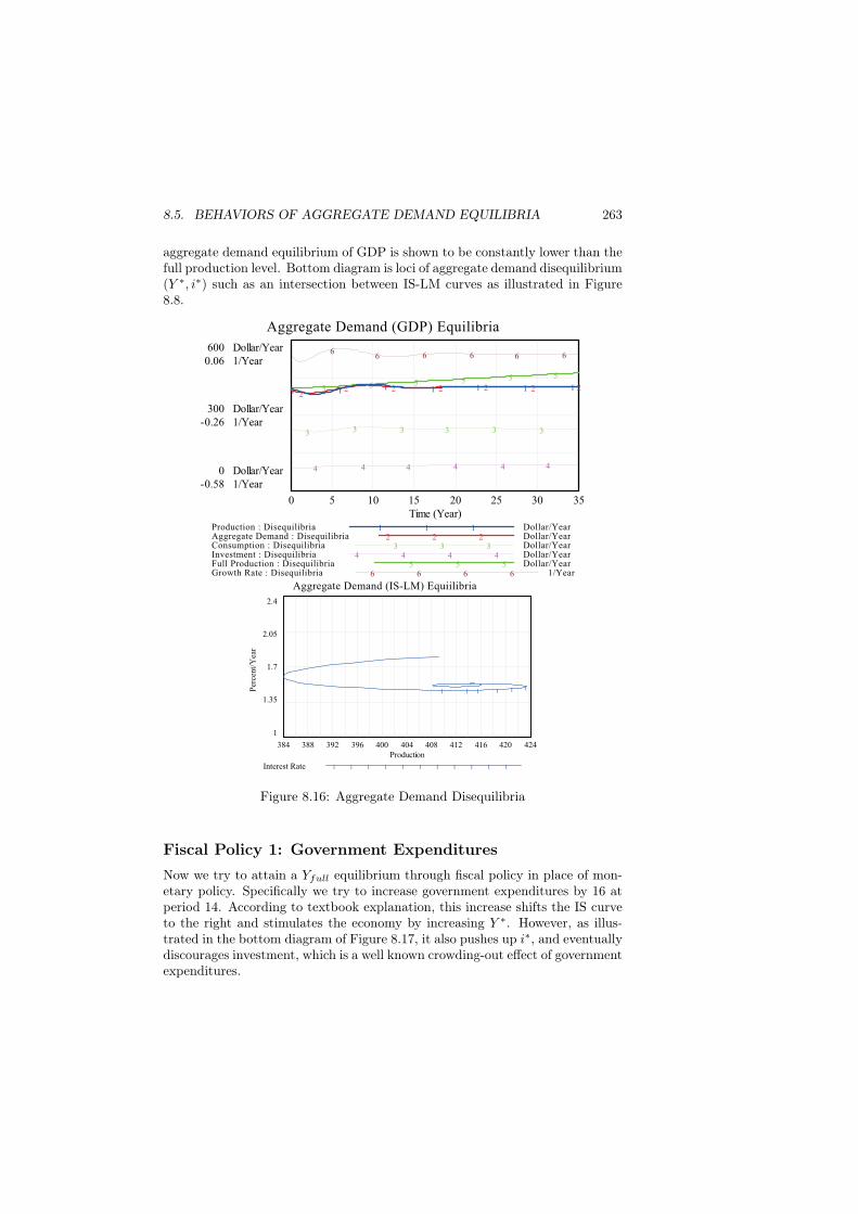
Here we consider a disequilibrium case which is triggered by changing theamount of basic consumption from 101 to 90. Top diagram in Figure 8.16 showsthat initial equilibrium amount of Y = 409.09 is thrown into disequilibrium untila discrepancy between full production and desired production is brought to anequilibrium about Y ∗ = 422 around the period 9 once again. Beyond thispoint, however, the economy is once again thrown into recession; that is to say,
8.5. BEHAVIORS OF AGGREGATE DEMAND EQUILIBRIA 263
aggregate demand equilibrium of GDP is shown to be constantly lower than thefull production level. Bottom diagram is loci of aggregate demand disequilibrium(Y ∗, i∗) such as an intersection between IS-LM curves as illustrated in Figure8.8.
Aggregate Demand (GDP) Equilibria
600 Dollar/Year0.06 1/Year
300 Dollar/Year-0.26 1/Year
0 Dollar/Year-0.58 1/Year
66 6 6 6 6
5 5 5 5 5 5
4 4 4 4 4 4
3 3 3 3 3 3
22 2 2 2 2 21 1 1 1 1 1 1
0 5 10 15 20 25 30 35Time (Year)
Production : Disequilibria Dollar/Year1 1 1Aggregate Demand : Disequilibria Dollar/Year2 2 2Consumption : Disequilibria Dollar/Year3 3 3Investment : Disequilibria Dollar/Year4 4 4 4Full Production : Disequilibria Dollar/Year5 5 5Growth Rate : Disequilibria 1/Year6 6 6 6
Aggregate Demand (IS-LM) Equiilibria
2.4
2.05
1.7
1.35
1
1 1 1 1 1 1
384 388 392 396 400 404 408 412 416 420 424Production
Per
cent/
Yea
r
Interest Rate 1 1 1 1 1 1 1 1 1 1 1
Figure 8.16: Aggregate Demand Disequilibria
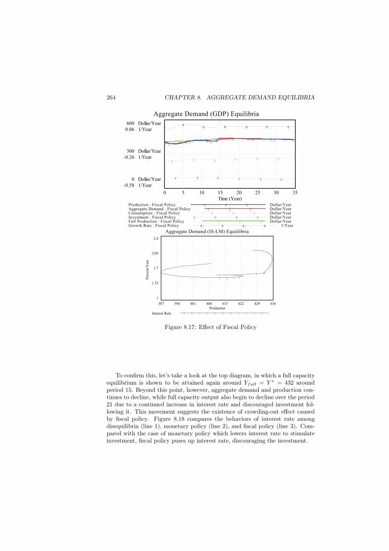
Fiscal Policy 1: Government ExpendituresNow we try to attain a Yfull equilibrium through fiscal policy in place of mon-etary policy. Specifically we try to increase government expenditures by 16 atperiod 14. According to textbook explanation, this increase shifts the IS curveto the right and stimulates the economy by increasing Y ∗. However, as illus-trated in the bottom diagram of Figure 8.17, it also pushes up i∗, and eventuallydiscourages investment, which is a well known crowding-out effect of governmentexpenditures.
264 CHAPTER 8. AGGREGATE DEMAND EQUILIBRIA
Aggregate Demand (GDP) Equilibria
600 Dollar/Year0.06 1/Year
300 Dollar/Year-0.26 1/Year
0 Dollar/Year-0.58 1/Year
66 6 6 6 6
5 5 5 5 5 5
4 4 4 4 4 4
3 3 3 3 3 3
22 2
2 2 2 21 1 1
1 1 1 1
0 5 10 15 20 25 30 35Time (Year)
Production : Fiscal Policy Dollar/Year1 1 1Aggregate Demand : Fiscal Policy Dollar/Year2 2 2Consumption : Fiscal Policy Dollar/Year3 3 3Investment : Fiscal Policy Dollar/Year4 4 4 4Full Production : Fiscal Policy Dollar/Year5 5 5Growth Rate : Fiscal Policy 1/Year6 6 6 6
Aggregate Demand (IS-LM) Equiilibria
2.4
2.05
1.7
1.35
1
1 1 1 11 11
1
387 394 401 408 415 422 429 436Production
Per
cent/
Yea
r
Interest Rate 1 1 1 1 1 1 1 1 1 1 1
Figure 8.17: Effect of Fiscal Policy
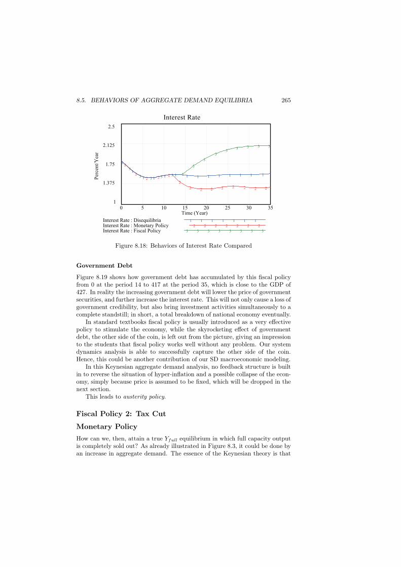
To confirm this, let’s take a look at the top diagram, in which a full capacityequilibrium is shown to be attained again around Yfull = Y ∗ = 432 aroundperiod 15. Beyond this point, however, aggregate demand and production con-tinues to decline, while full capacity output also begin to decline over the period21 due to a continued increase in interest rate and discouraged investment fol-lowing it. This movement suggests the existence of crowding-out effect causedby fiscal policy. Figure 8.18 compares the behaviors of interest rate amongdisequilibria (line 1), monetary policy (line 2), and fiscal policy (line 3). Com-pared with the case of monetary policy which lowers interest rate to stimulateinvestment, fiscal policy puses up interest rate, discouraging the investment.
8.5. BEHAVIORS OF AGGREGATE DEMAND EQUILIBRIA 265
Interest Rate
2.5
2.125
1.75
1.375
1
3
33 3 3 3
3
3
33
3 3 3 3
2
22 2
2
2
2 2 2 2 2 2 2 2
1
1
1 11 1 1 1 1 1 1 1 1 1
0 5 10 15 20 25 30 35Time (Year)
Per
cent/
Yea
r
Interest Rate : Disequilibria 1 1 1 1 1 1 1
Interest Rate : Monetary Policy 2 2 2 2 2 2 2
Interest Rate : Fiscal Policy 3 3 3 3 3 3 3 3
Figure 8.18: Behaviors of Interest Rate Compared
Government Debt
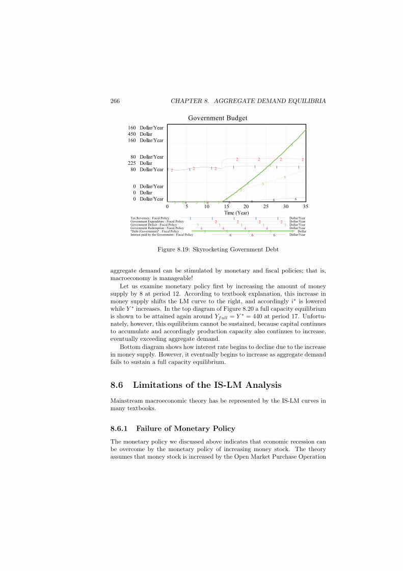
Figure 8.19 shows how government debt has accumulated by this fiscal policyfrom 0 at the period 14 to 417 at the period 35, which is close to the GDP of427. In reality the increasing government debt will lower the price of governmentsecurities, and further increase the interest rate. This will not only cause a loss ofgovernment credibility, but also bring investment activities simultaneously to acomplete standstill; in short, a total breakdown of national economy eventually.
In standard textbooks fiscal policy is usually introduced as a very effectivepolicy to stimulate the economy, while the skyrocketing effect of governmentdebt, the other side of the coin, is left out from the picture, giving an impressionto the students that fiscal policy works well without any problem. Our systemdynamics analysis is able to successfully capture the other side of the coin.Hence, this could be another contribution of our SD macroeconomic modeling.
In this Keynesian aggregate demand analysis, no feedback structure is builtin to reverse the situation of hyper-inflation and a possible collapse of the econ-omy, simply because price is assumed to be fixed, which will be dropped in thenext section.
This leads to austerity policy.
Fiscal Policy 2: Tax Cut
Monetary PolicyHow can we, then, attain a true Yfull equilibrium in which full capacity outputis completely sold out? As already illustrated in Figure 8.3, it could be done byan increase in aggregate demand. The essence of the Keynesian theory is that
266 CHAPTER 8. AGGREGATE DEMAND EQUILIBRIA
Government Budget
160 Dollar/Year450 Dollar160 Dollar/Year
80 Dollar/Year225 Dollar80 Dollar/Year
0 Dollar/Year0 Dollar0 Dollar/Year
6 6 6 6 6 65 5
5
5
5
5
3 3 3
3
3
3
2 2 2
2 2 2 2
1 1 1 1 1 1 1
0 5 10 15 20 25 30 35Time (Year)
Tax Revenues : Fiscal Policy Dollar/Year1 1 1 1 1Government Expenditure : Fiscal Policy Dollar/Year2 2 2 2Government Deficit : Fiscal Policy Dollar/Year3 3 3 3 3Government Redemption : Fiscal Policy Dollar/Year4 4 4 4"Debt (Government)" : Fiscal Policy Dollar5 5 5 5 5Interest paid by the Government : Fiscal Policy Dollar/Year6 6 6
Figure 8.19: Skyrocketing Government Debt
aggregate demand can be stimulated by monetary and fiscal policies; that is,macroeconomy is manageable!
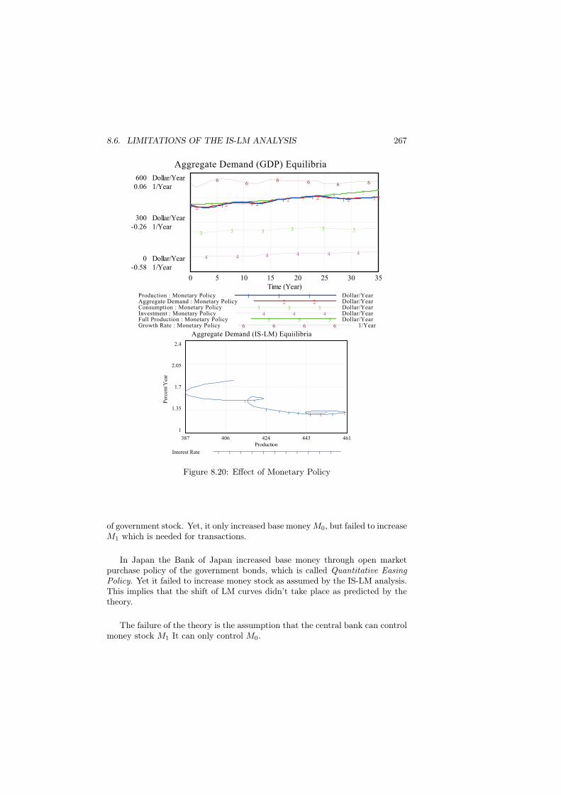
Let us examine monetary policy first by increasing the amount of moneysupply by 8 at period 12. According to textbook explanation, this increase inmoney supply shifts the LM curve to the right, and accordingly i∗ is loweredwhile Y ∗ increases. In the top diagram of Figure 8.20 a full capacity equilibriumis shown to be attained again around Yfull = Y ∗ = 440 at period 17. Unfortu-nately, however, this equilibrium cannot be sustained, because capital continuesto accumulate and accordingly production capacity also continues to increase,eventually exceeding aggregate demand.
Bottom diagram shows how interest rate begins to decline due to the increasein money supply. However, it eventually begins to increase as aggregate demandfails to sustain a full capacity equilibrium.
8.6 Limitations of the IS-LM Analysis
Mainstream macroeconomic theory has be represented by the IS-LM curves inmany textbooks.
8.6.1 Failure of Monetary Policy
The monetary policy we discussed above indicates that economic recession canbe overcome by the monetary policy of increasing money stock. The theoryassumes that money stock is increased by the Open Market Purchase Operation
8.6. LIMITATIONS OF THE IS-LM ANALYSIS 267
Aggregate Demand (GDP) Equilibria
600 Dollar/Year0.06 1/Year
300 Dollar/Year-0.26 1/Year
0 Dollar/Year-0.58 1/Year
66
6 6 6 6
5 5 55
55
4 4 4 4 4 4
3 3 3 3 3 3
22 2
2 2 2 2
1 1 11
1 1 1
0 5 10 15 20 25 30 35Time (Year)
Production : Monetary Policy Dollar/Year1 1 1Aggregate Demand : Monetary Policy Dollar/Year2 2Consumption : Monetary Policy Dollar/Year3 3 3Investment : Monetary Policy Dollar/Year4 4 4Full Production : Monetary Policy Dollar/Year5 5 5Growth Rate : Monetary Policy 1/Year6 6 6 6
Aggregate Demand (IS-LM) Equiilibria
2.4
2.05
1.7
1.35
1
1 1
11 1 1 1 1 1 1
387 406 424 443 461Production
Per
cent/
Yea
r
Interest Rate 1 1 1 1 1 1 1 1 1 1 1
Figure 8.20: Effect of Monetary Policy
of government stock. Yet, it only increased base money M0, but failed to increaseM1 which is needed for transactions.
In Japan the Bank of Japan increased base money through open marketpurchase policy of the government bonds, which is called Quantitative EasingPolicy. Yet it failed to increase money stock as assumed by the IS-LM analysis.This implies that the shift of LM curves didn’t take place as predicted by thetheory.
The failure of the theory is the assumption that the central bank can controlmoney stock M1 It can only control M0.
268 CHAPTER 8. AGGREGATE DEMAND EQUILIBRIA
8.6.2 Erroneous Money Hypothesis of the Great Depres-sion
When money stock shrinks, the LM curves shifts to the left, causing recession.Money Hypothesis claims that this has been the main cause of Great Depression.If this theory is correct, interest rate should have increased due to the shortageof money stock. Yet, interest rate dropped during the Great Depression. Thisindicates that Money Hypothesis failed to explain the behaviors of the GreatDepression.
True explanation is as follows. After the bubble burst, a rumor of bankruptcyspread, causing bank runs among depositors. This increases the liquidity pref-erences or cash ratio in Chapter 5, forcing the reserves by the banks. Under thefractional reserve banking system a tiny reduction of reserves multiple largerdeduction of deposits; that is, money stock as indicated in the Table on GreatDepression.
This decrease in money stock constrains the corporate and housing invest-ment, in spite of the decrease in interest rate. Hence, bubble burst decreasesmoney stock (shift of LM curve), then almost simultaneously decreases con-sumption and investment (shift of IS curves).
Irvins Fisher correctly pointed out the fractional reserve banking system as amain cause of the Great Depression. Hence, he advocated 100% reserve system,which turned into our analysis of the Public Money System in Part IV.
8.7 Neoclassical Policy of Price FlexibilityIt is now clear that the Keynesian theory of aggregate demand equilibria isimperfect from a SD model-building point of view, because price level is assumedto be sticky and there exists no built-in mechanism to restore a full capacityproduction equilibrium unless monetary and fiscal policies are carried out.
In fact, let us rewrite the aggregate demand equilibrium of GDP obtainedin equation (8.25) as a function of price:
Y ∗(P ) = A+BMs
PV, (8.37)
where A and B are combined constant amounts. Then it becomes clear thatthis equation only provides a relation between Y ∗ and P . Hence, Y ∗ is calledan aggregate demand function of price. It is now obvious that, unless price isflexible, there exists no mechanism to attain a true equilibrium such that
Yfull = Y ∗(P ) (8.38)
It is shown in the previous section that, even though monetary and fiscalpolicies can attain a full capacity production equilibrium, central bank and gov-ernment need to constantly fine-tune their policies to sustain such equilibrium.Can they really perform the task under a sticky price in the short run? If so,how short is a short run, practically speaking, to apply such policies?
8.7. NEOCLASSICAL POLICY OF PRICE FLEXIBILITY 269
From a dynamic point of view, it’s very hard to specify how short is a shortrun. Is this moment in the short run or in the long run? It depends on whento specify an initial point. This moment could be in the short run to justifycurrent policies. Or it could be already in the long run, and a long-run priceadjustment mechanism, to be discussed below, may be under way. If so, currentpolicy applications might worsen economic situations.
Accordingly, a better way of modeling a macroeconomic system has to allowprice flexibility in the model from the beginning and let the price adjust disequi-libria, including a fixed price as its special case. To do this formally, we have tobring a previously neglected equation (8.10). To avoid a redundancy of equationby doing so, we need to introduce another variable of price, and let it adjustdiscrepancies between full capacity output Yfull and desired production Y D asin the equation of price adjustment mechanism (8.11). Such discrepancies arecalled GDP gap. Price, however, may also adjust directly to the discrepanciesbetween inventory Inv and its desired inventory I∗nv, which are called inventorygap here. This is an adjustment process of attaining stability on a historicaltime already discussed in Chapter 2.
Hence, such an adjustment equation could be described as
dP
dt= Ψ(Y D − Yfull, I
∗nv − Inv). (8.39)
Let us specify the equation, as in the interest equation (8.33), as follows:
dP
dt=
P ∗ − P
Delay Time(8.40)
where the desired price P ∗ is obtained as
P ∗ =P(
(1− ω)Yfull
Y D + ω InvI∗nv
)e (8.41)
where ω, 0 ≤ ω ≤ 1, is a weight between production and inventory ratios, and eis an elasticity.
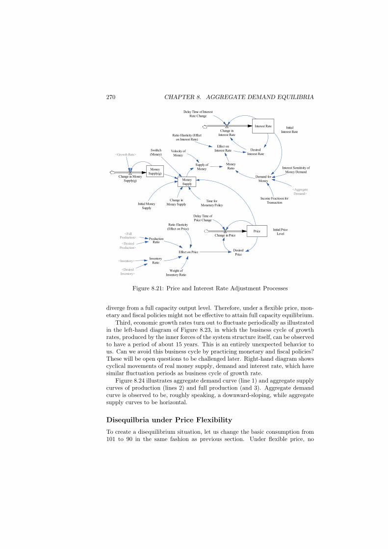
This completes our SD macroeconomic modeling of Keynesian IS-LM model.Figure 8.21 illustrates adjustment processes of price and interest rate.
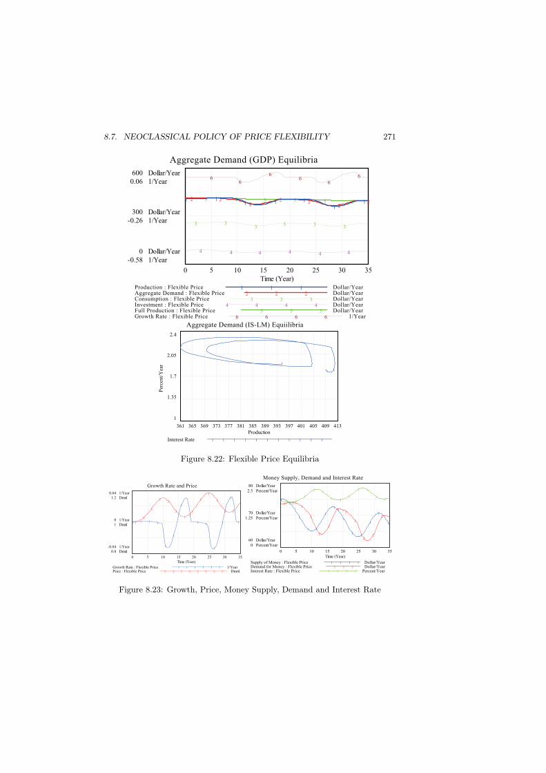
With the introduction of flexible price (which is attained by setting a ratioelasticity of effect on price = 1.0), behaviors of the model turns out to be sur-prisingly different from the previous model under a fixed price. First, aggregatedemand equilibrium, Y ∗, can no longer be attained as in the previous fixedprice case. Instead, as top diagram of Figure 8.22 illustrates, they fluctuatesalternatively, which we call aggregate demand alternations.
Second, this alternation moves along a full capacity output level, and oc-casionally approaches to a full capacity equilibrium such that Yfull = Y ∗ as ifbutterflies moves around flowers and occasionally rest on them. This vividlycontrast with the previous fixed price case in which aggregate demand equilib-rium can be attained through monetary and fiscal policies, but it will eventually
270 CHAPTER 8. AGGREGATE DEMAND EQUILIBRIA
Interest Rate
Change inInterest Rate
Demand forMoney
<AggregateDemand>
Interest Sensitivity ofMoney Demand
MoneySupply
Income Fractioon forTransaction
Delay Time of InterestRate Change
Initial MoneySupply
Change inMoney Supply
Time forMonetary Policy
PriceChange in Price
Delay Time ofPrice Change
Initial PriceLevel<Full
Production>
<DesiredProduction>
Velocity ofMoney
Supply ofMoneyMoney
Supply(g)Change in Money
Supply(g)
<Growth Rate>
Swithch(Money)
Effect on PriceDesired
Price
Weight ofInventory Ratio
ProductionRatio
<Inventory>
<DesiredInventory>
InventoryRatio
Ratio Elasticity(Effect on Price)
MoneyRatio
Effect onInterest Rate
Ratio Elasticity (Effecton Interest Rate)
DesiredInterest Rate
InitialInterest Rate
Figure 8.21: Price and Interest Rate Adjustment Processes
diverge from a full capacity output level. Therefore, under a flexible price, mon-etary and fiscal policies might not be effective to attain full capacity equilibrium.
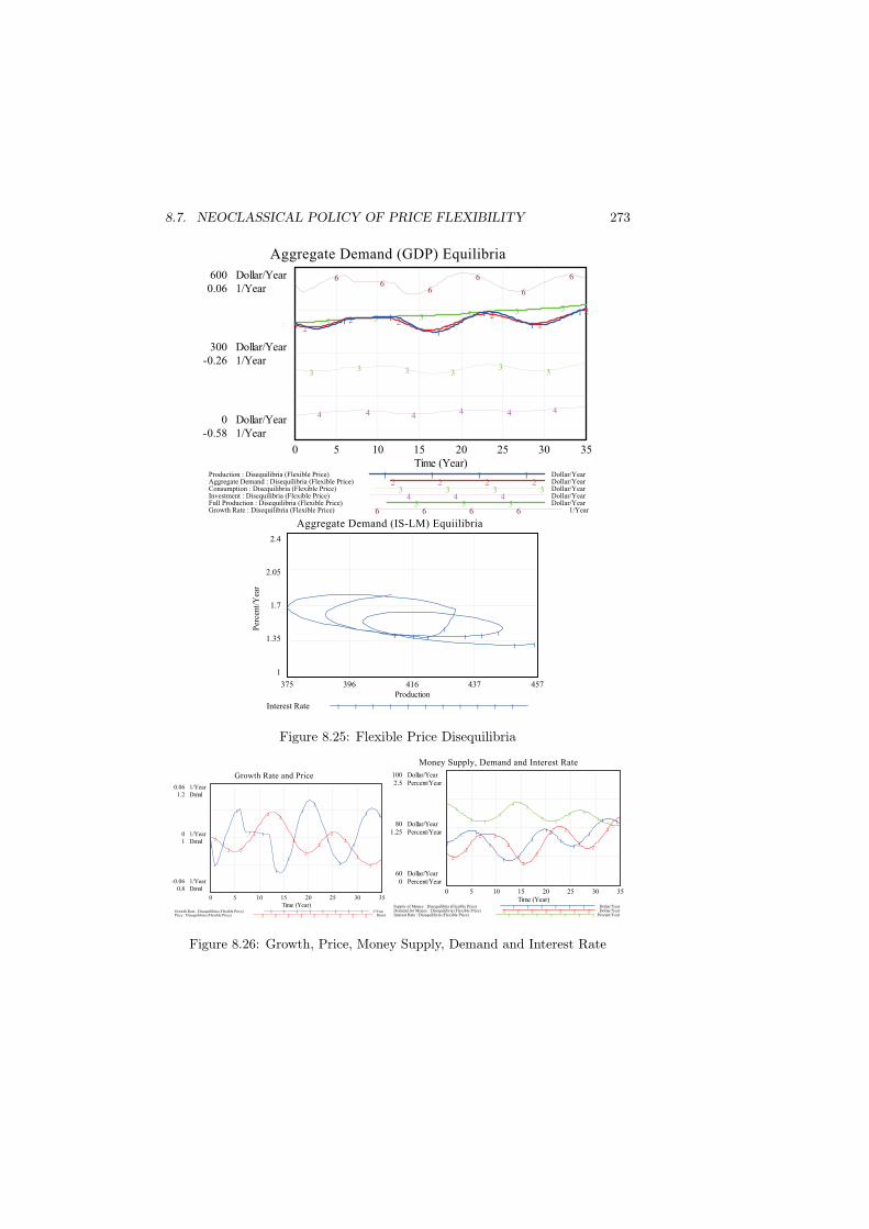
Third, economic growth rates turn out to fluctuate periodically as illustratedin the left-hand diagram of Figure 8.23, in which the business cycle of growthrates, produced by the inner forces of the system structure itself, can be observedto have a period of about 15 years. This is an entirely unexpected behavior tous. Can we avoid this business cycle by practicing monetary and fiscal policies?These will be open questions to be challenged later. Right-hand diagram showscyclical movements of real money supply, demand and interest rate, which havesimilar fluctuation periods as business cycle of growth rate.
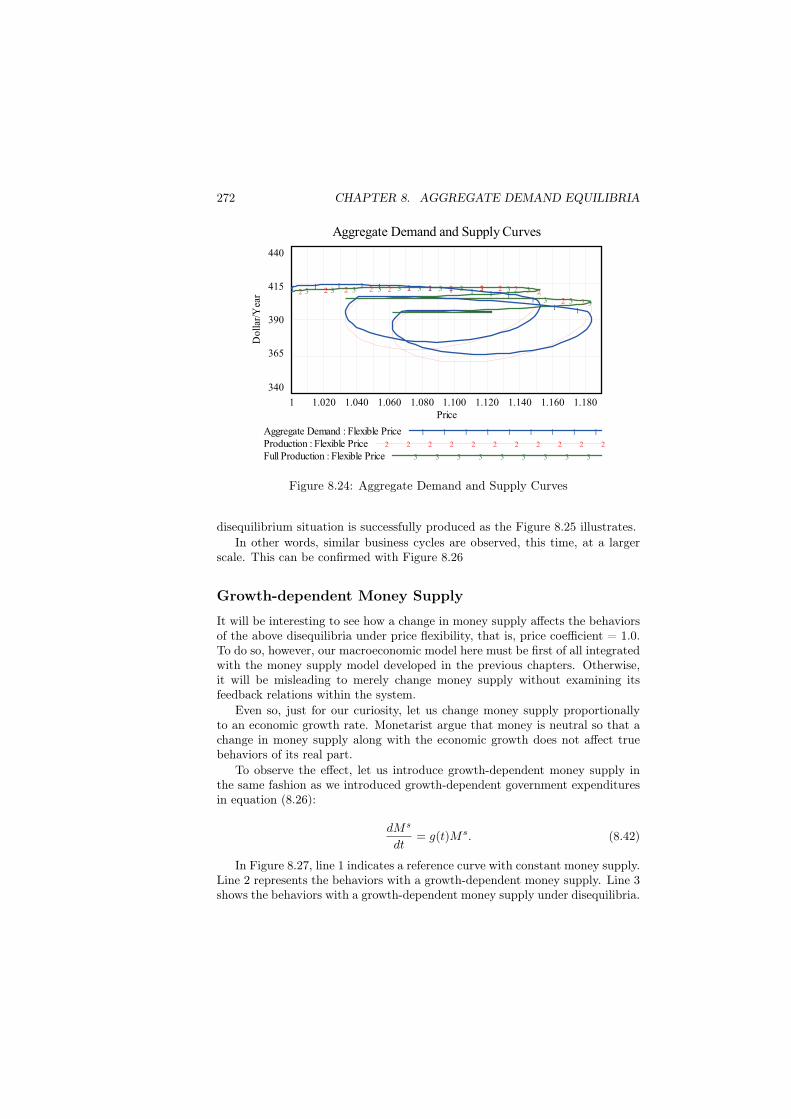
Figure 8.24 illustrates aggregate demand curve (line 1) and aggregate supplycurves of production (lines 2) and full production (and 3). Aggregate demandcurve is observed to be, roughly speaking, a downward-sloping, while aggregatesupply curves to be horizontal.
Disequilbria under Price FlexibilityTo create a disequilibrium situation, let us change the basic consumption from101 to 90 in the same fashion as previous section. Under flexible price, no
8.7. NEOCLASSICAL POLICY OF PRICE FLEXIBILITY 271
Aggregate Demand (GDP) Equilibria
600 Dollar/Year0.06 1/Year
300 Dollar/Year-0.26 1/Year
0 Dollar/Year-0.58 1/Year
66
66
66
5 5 5 5 5 5
4 4 4 4 4 4
3 33
3 3 3
2 22
2 22
21 11 1 1
11
0 5 10 15 20 25 30 35Time (Year)
Production : Flexible Price Dollar/Year1 1 1Aggregate Demand : Flexible Price Dollar/Year2 2 2Consumption : Flexible Price Dollar/Year3 3 3Investment : Flexible Price Dollar/Year4 4 4 4Full Production : Flexible Price Dollar/Year5 5 5Growth Rate : Flexible Price 1/Year6 6 6 6
Aggregate Demand (IS-LM) Equiilibria
2.4
2.05
1.7
1.35
1
1
361 365 369 373 377 381 385 389 393 397 401 405 409 413Production
Per
cent/
Yea
r
Interest Rate 1 1 1 1 1 1 1 1 1 1 1
Figure 8.22: Flexible Price Equilibria
Growth Rate and Price
0.04 1/Year1.2 Dmnl
0 1/Year1 Dmnl
-0.04 1/Year0.8 Dmnl
2
2
2
22
2
2
2
2
2
2
2 2
1 1 11
1
1
1
1
11
1
1
1
1
0 5 10 15 20 25 30 35Time (Year)
Growth Rate : Flexible Price 1/Year1 1 1 1 1 1
Price : Flexible Price Dmnl2 2 2 2 2 2 2 2
Money Supply, Demand and Interest Rate
80 Dollar/Year2.5 Percent/Year
70 Dollar/Year1.25 Percent/Year
60 Dollar/Year0 Percent/Year
3 3
3
33
33
3
3 3
33
2 22
2
2
2
22
2
22
2
1
1
1
1 1
1
1
1
11
1
1
1
0 5 10 15 20 25 30 35Time (Year)
Supply of Money : Flexible Price Dollar/Year1 1 1 1
Demand for Money : Flexible Price Dollar/Year2 2 2
Interest Rate : Flexible Price Percent/Year3 3 3 3
Figure 8.23: Growth, Price, Money Supply, Demand and Interest Rate
272 CHAPTER 8. AGGREGATE DEMAND EQUILIBRIA
Aggregate Demand and Supply Curves
440
415
390
365
340
3 3 3 3 3 3 3 3 3 3 3
3 3 3
2 2 2 2 2 2 2 2 2 2 2 22 2
1 1 1 1 1 1 1 1 1 1 11
1 1
1 1.020 1.040 1.060 1.080 1.100 1.120 1.140 1.160 1.180Price
Do
llar
/Yea
r
Aggregate Demand : Flexible Price 1 1 1 1 1 1 1 1 1
Production : Flexible Price 2 2 2 2 2 2 2 2 2 2 2
Full Production : Flexible Price 3 3 3 3 3 3 3 3 3
Figure 8.24: Aggregate Demand and Supply Curves
disequilibrium situation is successfully produced as the Figure 8.25 illustrates.In other words, similar business cycles are observed, this time, at a larger
scale. This can be confirmed with Figure 8.26
Growth-dependent Money Supply
It will be interesting to see how a change in money supply affects the behaviorsof the above disequilibria under price flexibility, that is, price coefficient = 1.0.To do so, however, our macroeconomic model here must be first of all integratedwith the money supply model developed in the previous chapters. Otherwise,it will be misleading to merely change money supply without examining itsfeedback relations within the system.
Even so, just for our curiosity, let us change money supply proportionallyto an economic growth rate. Monetarist argue that money is neutral so that achange in money supply along with the economic growth does not affect truebehaviors of its real part.
To observe the effect, let us introduce growth-dependent money supply inthe same fashion as we introduced growth-dependent government expendituresin equation (8.26):
dMs
dt= g(t)Ms. (8.42)
In Figure 8.27, line 1 indicates a reference curve with constant money supply.Line 2 represents the behaviors with a growth-dependent money supply. Line 3shows the behaviors with a growth-dependent money supply under disequilibria.
8.7. NEOCLASSICAL POLICY OF PRICE FLEXIBILITY 273
Aggregate Demand (GDP) Equilibria
600 Dollar/Year0.06 1/Year
300 Dollar/Year-0.26 1/Year
0 Dollar/Year-0.58 1/Year
66
6
6
6
6
5 5 5 5 5 5
4 4 44 4 4
33 3 3
33
22 2
2
22
2
1 1 1
1
1
1
1
0 5 10 15 20 25 30 35Time (Year)
Production : Disequilibria (Flexible Price) Dollar/Year1 1 1 1Aggregate Demand : Disequilibria (Flexible Price) Dollar/Year2 2 2 2Consumption : Disequilibria (Flexible Price) Dollar/Year3 3 3 3Investment : Disequilibria (Flexible Price) Dollar/Year4 4 4Full Production : Disequilibria (Flexible Price) Dollar/Year5 5 5Growth Rate : Disequilibria (Flexible Price) 1/Year6 6 6 6
Aggregate Demand (IS-LM) Equiilibria
2.4
2.05
1.7
1.35
1
1 1 1
11 1 1
1 1
375 396 416 437 457Production
Per
cent/
Yea
r
Interest Rate 1 1 1 1 1 1 1 1 1 1 1
Figure 8.25: Flexible Price Disequilibria
Growth Rate and Price
0.06 1/Year1.2 Dmnl
0 1/Year1 Dmnl
-0.06 1/Year0.8 Dmnl
2
2 2
2
22
2
2
2
2
2
2
2
11
1
1 1
1
1
1
1
1
1
1
1 1
0 5 10 15 20 25 30 35Time (Year)
Growth Rate : Disequilibria (Flexible Price) 1/Year1 1 1 1 1 1 1 1Price : Disequilibria (Flexible Price) Dmnl2 2 2 2 2 2 2 2 2
Money Supply, Demand and Interest Rate
100 Dollar/Year2.5 Percent/Year
80 Dollar/Year1.25 Percent/Year
60 Dollar/Year0 Percent/Year
3
3 3
3
33
33
33
3
3
2
2
2 2
2
2
2
22
22
2
1
11
1
11
1
1
11
1
1 1
0 5 10 15 20 25 30 35Time (Year)
Supply of Money : Disequilibria (Flexible Price) Dollar/Year1 1 1 1 1 1Demand for Money : Disequilibria (Flexible Price) Dollar/Year2 2 2 2 2 2 2Interest Rate : Disequilibria (Flexible Price) Percent/Year3 3 3 3 3 3 3
Figure 8.26: Growth, Price, Money Supply, Demand and Interest Rate
274 CHAPTER 8. AGGREGATE DEMAND EQUILIBRIA
Supply of Money
100
85
70
55
40
33
3 3
3
33
3
3
3
33
33
22
2
22
22
2
22
2
2
22
1 11
11
1
11
1
11
1
1 11
0 5 10 15 20 25 30 35Time (Year)
Doll
ar/Y
ear
Supply of Money : Flexible Price 1 1 1 1 1 1 1 1 1 1 1Supply of Money : Money Supply (Growth) 2 2 2 2 2 2 2 2 2 2Supply of Money : Money Supply (Disequilibria) 3 3 3 3 3 3 3 3
Interest Rate
4
3
2
1
0
33
3 3 33
33 3
33
3 3 33
2 2 22
22 2
22
2 2
2
22
2
1 1 11
11
11 1
1
11
11 1
0 5 10 15 20 25 30 35Time (Year)
Per
cent/
Yea
r
Interest Rate : Flexible Price 1 1 1 1 1 1 1 1 1 1 1Interest Rate : Money Supply (Growth) 2 2 2 2 2 2 2 2 2 2Interest Rate : Money Supply (Disequilibria) 3 3 3 3 3 3 3 3 3
Figure 8.27: Growth-dependent Money Supply and its Effect on Interest Rate
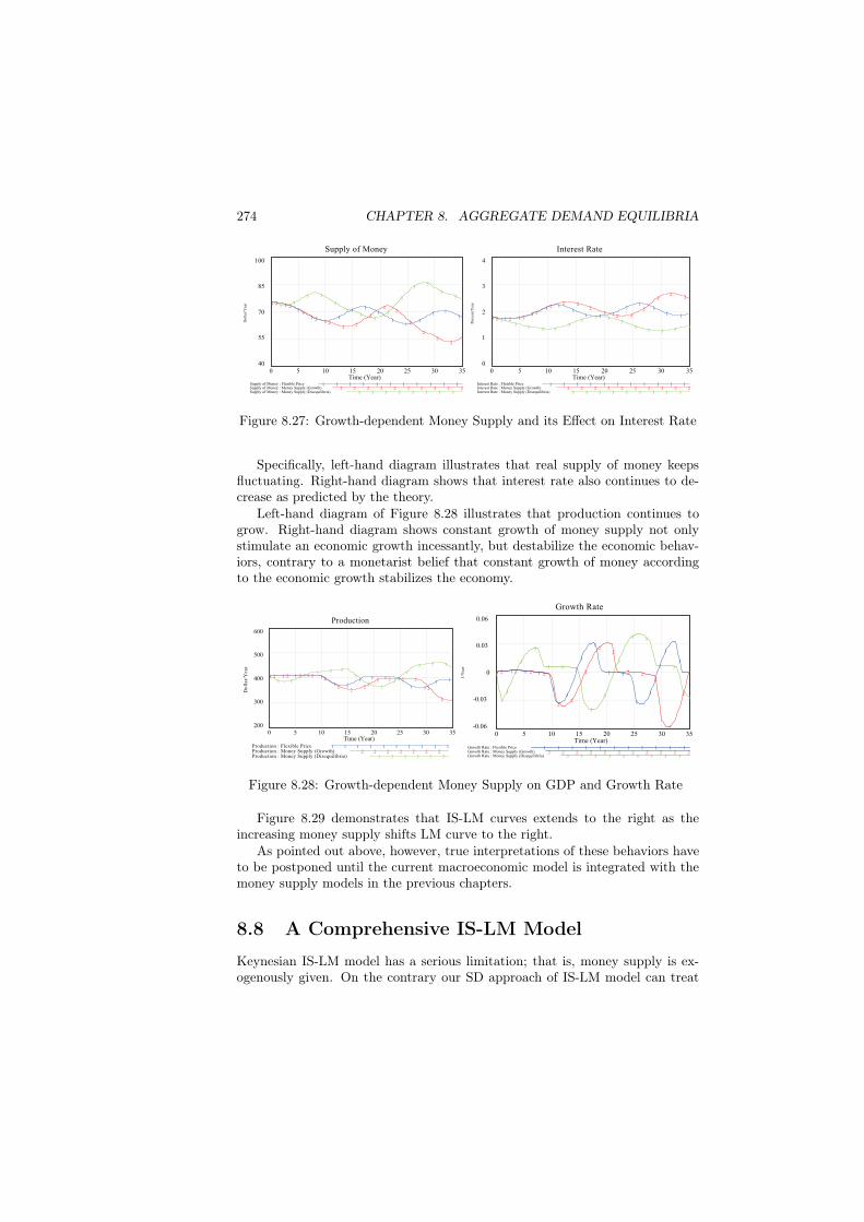
Specifically, left-hand diagram illustrates that real supply of money keepsfluctuating. Right-hand diagram shows that interest rate also continues to de-crease as predicted by the theory.
Left-hand diagram of Figure 8.28 illustrates that production continues togrow. Right-hand diagram shows constant growth of money supply not onlystimulate an economic growth incessantly, but destabilize the economic behav-iors, contrary to a monetarist belief that constant growth of money accordingto the economic growth stabilizes the economy.
Production
600
500
400
300
200
3 33
3 3 3
3
33
3
3
3 3 3
2 2 2 22
22
2
2 2 2 2
2
2
1 1 1 1 1
1 11
1 1 1
1 1
1 1
0 5 10 15 20 25 30 35Time (Year)
Do
llar
/Yea
r
Production : Flexible Price 1 1 1 1 1 1 1 1 1 1Production : Money Supply (Growth) 2 2 2 2 2 2 2Production : Money Supply (Disequilibria) 3 3 3 3 3 3
Growth Rate
0.06
0.03
0
-0.03
-0.06
3
3
3
3 3 3
3
3
3
3 3
3 3
3
2 2 2 2
22
2
22
2 22
2
2
1 1 1 1
11
1
1
1 1
1
1
1
1
0 5 10 15 20 25 30 35Time (Year)
1/Y
ear
Growth Rate : Flexible Price 1 1 1 1 1 1 1 1 1 1 1Growth Rate : Money Supply (Growth) 2 2 2 2 2 2 2 2 2 2 2Growth Rate : Money Supply (Disequilibria) 3 3 3 3 3 3 3 3 3
Figure 8.28: Growth-dependent Money Supply on GDP and Growth Rate
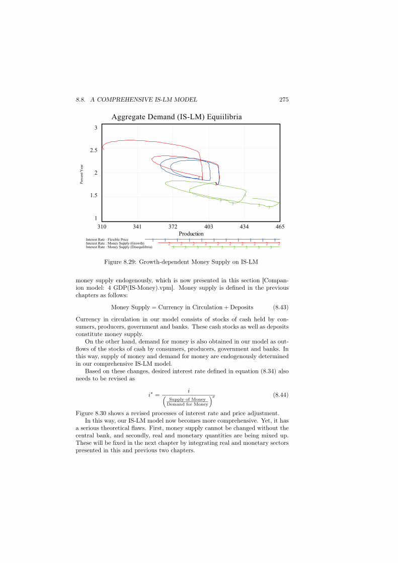
Figure 8.29 demonstrates that IS-LM curves extends to the right as theincreasing money supply shifts LM curve to the right.
As pointed out above, however, true interpretations of these behaviors haveto be postponed until the current macroeconomic model is integrated with themoney supply models in the previous chapters.
8.8 A Comprehensive IS-LM ModelKeynesian IS-LM model has a serious limitation; that is, money supply is ex-ogenously given. On the contrary our SD approach of IS-LM model can treat
8.8. A COMPREHENSIVE IS-LM MODEL 275
Aggregate Demand (IS-LM) Equiilibria
3
2.5
2
1.5
1
33
3
33
2
310 341 372 403 434 465Production
Per
cen
t/Y
ear
Interest Rate : Flexible Price 1 1 1 1 1 1 1 1 1 1 1Interest Rate : Money Supply (Growth) 2 2 2 2 2 2 2 2 2 2Interest Rate : Money Supply (Disequilibria) 3 3 3 3 3 3 3 3 3
Figure 8.29: Growth-dependent Money Supply on IS-LM
money supply endogenously, which is now presented in this section [Compan-ion model: 4 GDP(IS-Money).vpm]. Money supply is defined in the previouschapters as follows:
Money Supply = Currency in Circulation + Deposits (8.43)
Currency in circulation in our model consists of stocks of cash held by con-sumers, producers, government and banks. These cash stocks as well as depositsconstitute money supply.
On the other hand, demand for money is also obtained in our model as out-flows of the stocks of cash by consumers, producers, government and banks. Inthis way, supply of money and demand for money are endogenously determinedin our comprehensive IS-LM model.
Based on these changes, desired interest rate defined in equation (8.34) alsoneeds to be revised as
i∗ =i(
Supply of MoneyDemand for Money
)e (8.44)
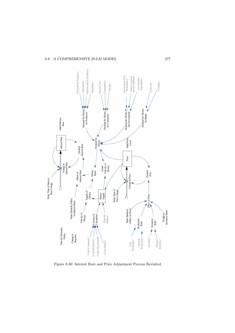
Figure 8.30 shows a revised processes of interest rate and price adjustment.In this way, our IS-LM model now becomes more comprehensive. Yet, it has
a serious theoretical flaws. First, money supply cannot be changed without thecentral bank, and secondly, real and monetary quantities are being mixed up.These will be fixed in the next chapter by integrating real and monetary sectorspresented in this and previous two chapters.
276 CHAPTER 8. AGGREGATE DEMAND EQUILIBRIA
Even so, it’s worth a while to observe how our comprehensive SD modelbehaves in comparison with a traditional Keynesian IS-LM model presentedabove.
Behaviors of the modelIn the model aggregate demand equilibria are attained by setting a value ofvelocity of money to be 0.52, with all other model values remaining the sameas before.
One of the Disequilibria can be triggered, as before, by reducing the amountof basic consumption from 101. Equilibria can be restored by introducing fis-cal policy as before, with a skyrocketing government debt accumulated. Thissimulation is left to the reader.
There is no way, however, of introducing monetary policy in our model,simply because no central bank exists to create money supply within the system.
8.8. A COMPREHENSIVE IS-LM MODEL 277In
tere
st R
ate
Cha
nge
inIn
tere
st R
ate
Dem
and
fo
rM
one
yM
one
yS
upp
ly
Del
ay T
ime
of
Inte
rest
Rat
e C
hang
e
Cha
nge
inD
eposi
ts
Tim
e fo
r M
one
tary
Po
licy
Pri
ceC
hang
e in
Pri
ce
Del
ay T
ime
of
Pri
ce C
hang
e
Initi
al P
rice
Lev
el<
Ful
lP
rod
uctio
n>
<D
esir
edP
rod
uctio
n>
Vel
oci
ty o
fM
one
yS
upp
ly o
fM
one
y
Dem
and
fo
r M
one
yb
y P
rod
ucer
s
Dem
and
fo
r M
one
yb
y C
ons
umer
s
Dem
and f
or
Mo
ney
by
the
Go
vern
men
t
<P
aym
ent
by
Pro
duc
er>
<In
vest
men
t>
<In
tere
st p
aid
by
Pro
duc
er>
<D
ivid
end
s>
<In
com
e T
ax>
<C
ons
ump
tion>
<G
ove
rnm
ent
Deb
tR
edem
ptio
n>
<In
tere
st p
aid
by
the
Go
vern
men
t>
<G
ove
rnm
ent
Exp
end
iture
>
Cur
renc
y in
Cir
cula
tion
<C
ash
(Cons
umer
)>
<C
ash
(Go
vern
men
t)>
<C
ash
(Pro
duc
er)>
<D
epo
sits
(Ban
ks)
>
Act
ual
Vel
oci
ty o
fM
one
y<
Sav
ing>
Mo
ney
Rat
io
Eff
ect
on
Inte
rest
Rat
e
Rat
io E
last
icity
(E
ffec
to
n In
tere
st R
ate)
Des
ired
Inte
rest
Rat
e
Initi
al I
nter
est
Rat
e
Pro
duc
tion
Rat
io
Inve
nto
ryR
atio
<In
vent
ory
>
<D
esir
edIn
vent
ory
>
Eff
ect
on
Pri
ce
Wei
ght
of
Inve
nto
ry R
atio
Rat
io E
last
icity
(Eff
ect
on
Pri
ce)
Des
ired
Pri
ce
<C
ash
(Ban
ks)
>
Dem
and
fo
r M
one
yb
y B
ank
s
<C
ash
out
>
<L
end
ing>
Figure 8.30: Interest Rate and Price Adjustment Process Revisited
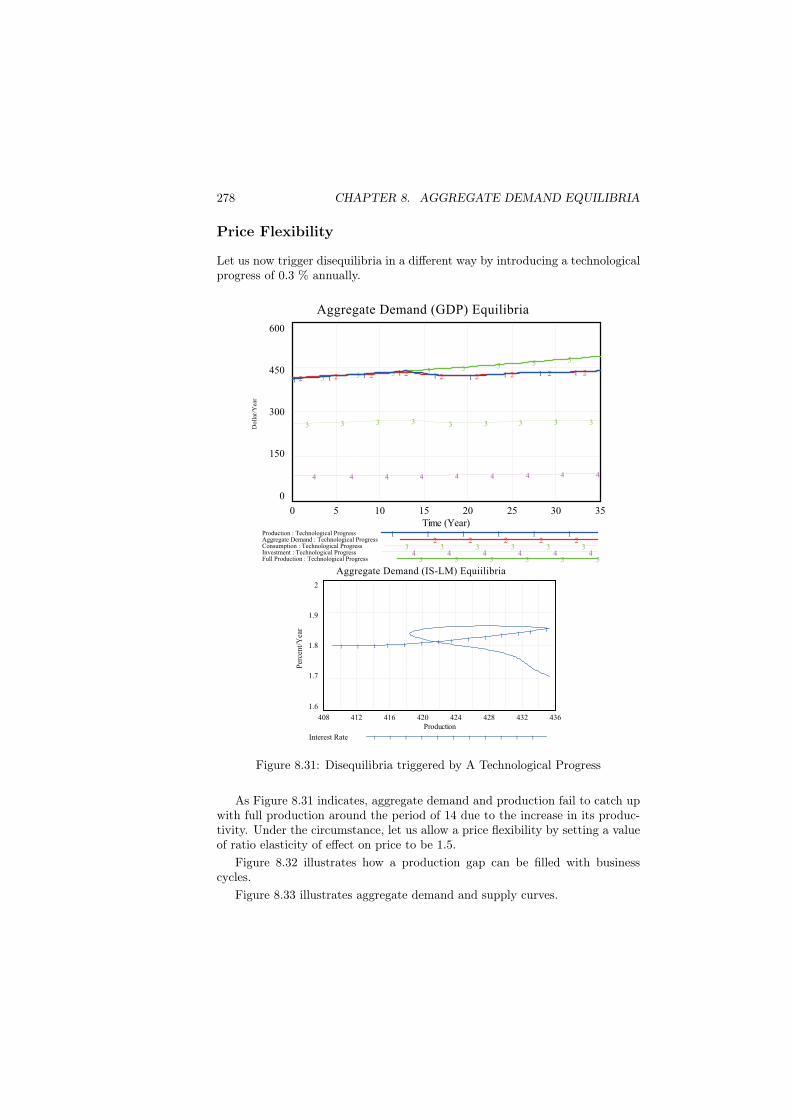
278 CHAPTER 8. AGGREGATE DEMAND EQUILIBRIA
Price Flexibility
Let us now trigger disequilibria in a different way by introducing a technologicalprogress of 0.3 % annually.
Aggregate Demand (GDP) Equilibria
600
450
300
150
0
5 5 5 5 5 5 5 5
4 4 4 4 4 4 4 4 4
3 3 3 3 3 3 3 3 3
2 2 2 2 2 2 2 2 21 1 1 1 1 1 1 1 1
0 5 10 15 20 25 30 35Time (Year)
Do
llar
/Yea
r
Production : Technological Progress 1 1 1 1 1 1Aggregate Demand : Technological Progress 2 2 2 2 2Consumption : Technological Progress 3 3 3 3 3 3Investment : Technological Progress 4 4 4 4 4 4Full Production : Technological Progress 5 5 5 5 5 5
Aggregate Demand (IS-LM) Equiilibria
2
1.9
1.8
1.7
1.6
1 1 1 1 1 1 1 1 1 1 1 1 1 1
408 412 416 420 424 428 432 436Production
Per
cent/
Yea
r
Interest Rate 1 1 1 1 1 1 1 1 1 1 1
Figure 8.31: Disequilibria triggered by A Technological Progress
As Figure 8.31 indicates, aggregate demand and production fail to catch upwith full production around the period of 14 due to the increase in its produc-tivity. Under the circumstance, let us allow a price flexibility by setting a valueof ratio elasticity of effect on price to be 1.5.
Figure 8.32 illustrates how a production gap can be filled with businesscycles.
Figure 8.33 illustrates aggregate demand and supply curves.
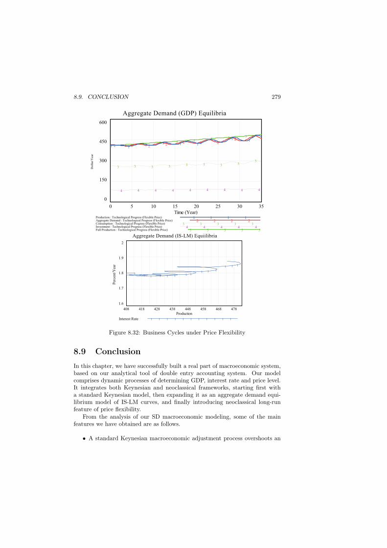
8.9. CONCLUSION 279
Aggregate Demand (GDP) Equilibria
600
450
300
150
0
5 5 5 5 5 5 5 5
4 4 4 4 4 4 4 4 4
3 3 3 3 3 3 3 33
2 2 22
2 2 22
2
1 11
1 1 11
11
0 5 10 15 20 25 30 35Time (Year)
Do
llar
/Yea
r
Production : Technological Progress (Flexible Price) 1 1 1 1Aggregate Demand : Technological Progress (Flexible Price) 2 2 2 2Consumption : Technological Progress (Flexible Price) 3 3 3 3 3Investment : Technological Progress (Flexible Price) 4 4 4 4 4Full Production : Technological Progress (Flexible Price) 5 5 5 5 5
Aggregate Demand (IS-LM) Equiilibria
2
1.9
1.8
1.7
1.6
11 1 1 1 1 1 1
1 1 1
1 1 1
408 418 428 438 448 458 468 478Production
Per
cen
t/Y
ear
Interest Rate 1 1 1 1 1 1 1 1 1 1 1
Figure 8.32: Business Cycles under Price Flexibility
8.9 ConclusionIn this chapter, we have successfully built a real part of macroeconomic system,based on our analytical tool of double entry accounting system. Our modelcomprises dynamic processes of determining GDP, interest rate and price level.It integrates both Keynesian and neoclassical frameworks, starting first witha standard Keynesian model, then expanding it as an aggregate demand equi-librium model of IS-LM curves, and finally introducing neoclassical long-runfeature of price flexibility.
From the analysis of our SD macroeconomic modeling, some of the mainfeatures we have obtained are as follows.
• A standard Keynesian macroeconomic adjustment process overshoots an
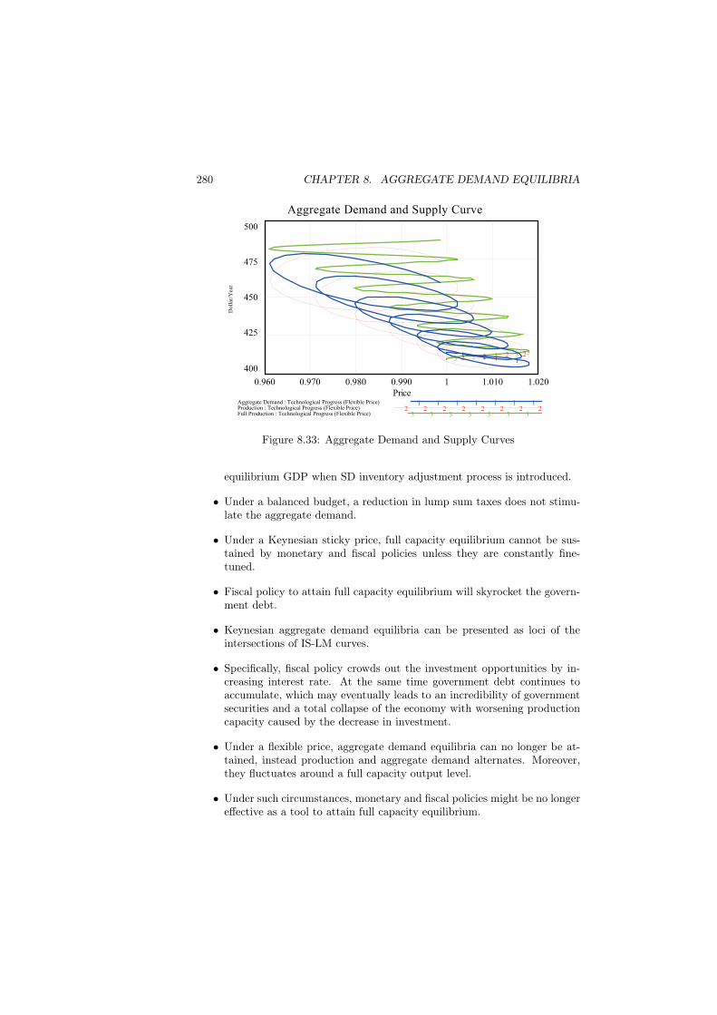
280 CHAPTER 8. AGGREGATE DEMAND EQUILIBRIA
Aggregate Demand and Supply Curve
500
475
450
425
4003 3 3 3 3
2 2 2 21 1 1 1
0.960 0.970 0.980 0.990 1 1.010 1.020Price
Doll
ar/Y
ear
Aggregate Demand : Technological Progress (Flexible Price) 1 1 1 1 1 1 1Production : Technological Progress (Flexible Price) 2 2 2 2 2 2 2 2Full Production : Technological Progress (Flexible Price) 3 3 3 3 3 3 3
Figure 8.33: Aggregate Demand and Supply Curves
equilibrium GDP when SD inventory adjustment process is introduced.
• Under a balanced budget, a reduction in lump sum taxes does not stimu-late the aggregate demand.
• Under a Keynesian sticky price, full capacity equilibrium cannot be sus-tained by monetary and fiscal policies unless they are constantly fine-tuned.
• Fiscal policy to attain full capacity equilibrium will skyrocket the govern-ment debt.
• Keynesian aggregate demand equilibria can be presented as loci of theintersections of IS-LM curves.
• Specifically, fiscal policy crowds out the investment opportunities by in-creasing interest rate. At the same time government debt continues toaccumulate, which may eventually leads to an incredibility of governmentsecurities and a total collapse of the economy with worsening productioncapacity caused by the decrease in investment.
• Under a flexible price, aggregate demand equilibria can no longer be at-tained, instead production and aggregate demand alternates. Moreover,they fluctuates around a full capacity output level.
• Under such circumstances, monetary and fiscal policies might be no longereffective as a tool to attain full capacity equilibrium.
8.9. CONCLUSION 281
• When money supply is fixed under a flexible price, price and interest ratecontinue to fluctuate.
• When money supply is changed proportionately to an economic growthrate, price and interest rate, as well as real money supply, begin to fluc-tuate larger than in the fixed money supply. Moreover, price and interestrate fluctuates oppositely to money supply.
• Keynesian IS-LM model thus presented above has a serious limitation;that is, money supply is exogenously given.
It may be too early to confirm some of the above features until we integratethe model presented in this chapter with the model of money supply in theprevious two chapters, because an endogenous change in money supply maytrigger an overall feedback reactions among all macroeconomic sectors, and themechanistic change in money supply introduced here might be misleading.
Apparently, this leads to our next target toward the integration of the realand monetary economic models developed so far.
282 CHAPTER 8. AGGREGATE DEMAND EQUILIBRIA
Questions for Deeper Understanding1. In the companion model: 2 Keynesian(SD).vpm, the equilibrium GDP is
assumed to be attained at GDP = 500. Suppose the full employment GDPis to be realized at GDP = 550; that is, the net increase in GDP of 50 hasto be added to the current level of GDP.a) Discuss how this can be done by running simulations. List as manypolicies as theoretically possible.b) From the list, pick up the most feasible policies to stimulate the econ-omy in your country and discuss why.
2. Figure 8.3 illustrates how GDP is determined by the amount of aggregatedemand. This is a method of the so-called Comparative Static Analysiswhich is heavily used in standard macroeconomic textbooks. Accordingto it, in order to increase GDP, it is not necessary to increase the sameamount of aggregate demand, say, government expenditures, due to themultiplier effect such that
∆GDP =1
1− c∆G
For instance, when c = 0.6, the multiplier of the government expendituresbecomes 2.5 so that to increase GDP by ∆GDP = 50, the governmentneeds to spend only ∆G = 20. This explanation gives us an incorrect im-pression that one time government expenditure attains a new equilibriumGDP. Using the above Keynesian SD model, discuss how comparativestatic analysis leads to such misperception of GDP determination.
3. Equilibrium GDP is obtained as Y ∗ in the equation (8.12). Calculate MPCelasticity of equilibrium GDP (≡ dY ∗
Y ∗ /dcc ). Then, re-build the Keynesian
model: 2 Keynesian(SD).vpm by adding this MPC elasticity to the model,and show how the MPC elasticity is affected by the changes in aggregatedemand; specifically, by tax cut. This may suggest the existence of amissing feedback loop from Change in Tax to Change in MPC in ourKeynesian SD model such that
Change in Tax =⇒ Change in MPC −→ Consumption −→ GDP.In other words, tax cut may have more positive impact on GDP thangenerally considered by the standard Keynesian models.
4. Balance sheet of producers in the model: 3 GDP(IS-LM).vpm is slightlydifferent from the simplified corporate balance sheet in Chapter 3 in theway inventory and account receivable are treated. Discuss why?
5. (Fiscal and Monetary Policies by IS-LM Approach)Traditional Keynesian IS-LM model is thoroughly reconstructed by theASD Keynesian macroeconomic model: 3 GDP(IS-LM).vpm. This ASDmodel can easily trigger recessions out of the equilibrium state. A typical
8.9. CONCLUSION 283
case of such recessions, called underconsumption recession here, can betriggered by reducing the amount of basic consumption by - 20 at t = 4under fixprice setting.Run the model and show how the equilibrium can be restored out of theunderconsumption recession by Keynesian fiscal and monetary policies.Equilibrium state is defined as
Full Production = Production = Aggregate Demand.Fiscal policies can be more specifically implemented by the changes in
(1) Government Expenditure(2) Lump-sum Taxes(3) Excise Tax Rate, and(4) Income Tax Rate.
Monetary policy can be implemented by the change in
(5) Money Supply.
Neoclassical theory proposes that the equilibrium can be restored by in-troducing
(6) Flexible Price.
The ASD Keynesian model can handle these 6 macroeconomic policies ina uniform fashion. Show how these 6 policies can attain the equilibrium,one by one, by illustrating simulation results in the graph titled: ʠFullProduction, Production & Aggregate Demandʡwhich is included in thethree simulation pages of the model. Then, summarize these 6 policies byintegrating all of them as graphs of Interest Rate and Debt (Government),and briefly compare them.
6. (Limitations of the IS-LM model by the Mainstream Theory)The IS-LM framework has been the dominant approach to Keynesianmacroeconomic theory. Yet, two theoretical limitations have been pointedout recently as follows:
(a) As a main cause of the Great Depression in 1929, Milton Friedmanand Anna Schwartz presented the decline of money supply by 25%from 1929 to 1933. This is a well-acknowledgedʠmoney hypothesisʡ.Yet, Mankiw pointed out as follows:ʠUsing the IS-LM model, we might interpret the moneyhypothesis as explaining the Depression by a contractionaryshift in the LM curve. ʜThe second problem for the money hypothesis is the behav-ior of interest rates. If a contractionary shift in the LM curvetriggered the Depression, we should have observed higher in-terest rates.Yet nominal interest rates fell continuously from
284 CHAPTER 8. AGGREGATE DEMAND EQUILIBRIA
1929 to 1933."– Macroeconomics, 9th edition, 2016, by Gregory Mankiw,page 354 –
(b) After her bubble burst in mid 1990ʟs, Japanese economy has beensuffering from the prolonged recessions of almost three decades. Toget out of the recessions, Japanese government as well as the Bank ofJapan have heavily applied the Keynesian monetary policy of increas-ing money supply which is dubbed as Quantitative Easing policy. Asyou have run simulations above, this QE policy shifts the LM curveto the right and stimulates GDP. In reality, however, it didnʟt workas predicted by the theory.
Consequently, the IS-LM model has failed to explain these two observa-tions of the economic recessions. In other words, there exist some theoret-ical limitations to the IS-LM model as macroeconomic policy tools. Underthe circumstances, answer the following two questions.(A) Reproduce the Mankiwʟs assertion (a) above by running the ASDmodel, and discuss whatʟs wrong with the IS-LM approach of macroeco-nomic monetary policies.Tip: Reduce money supply by - 10 at t = 4.(B) Discuss why the shift of LM curve (that is, QE policy) didnʟt workas expected by the IS-LM model in the Japanese economy.
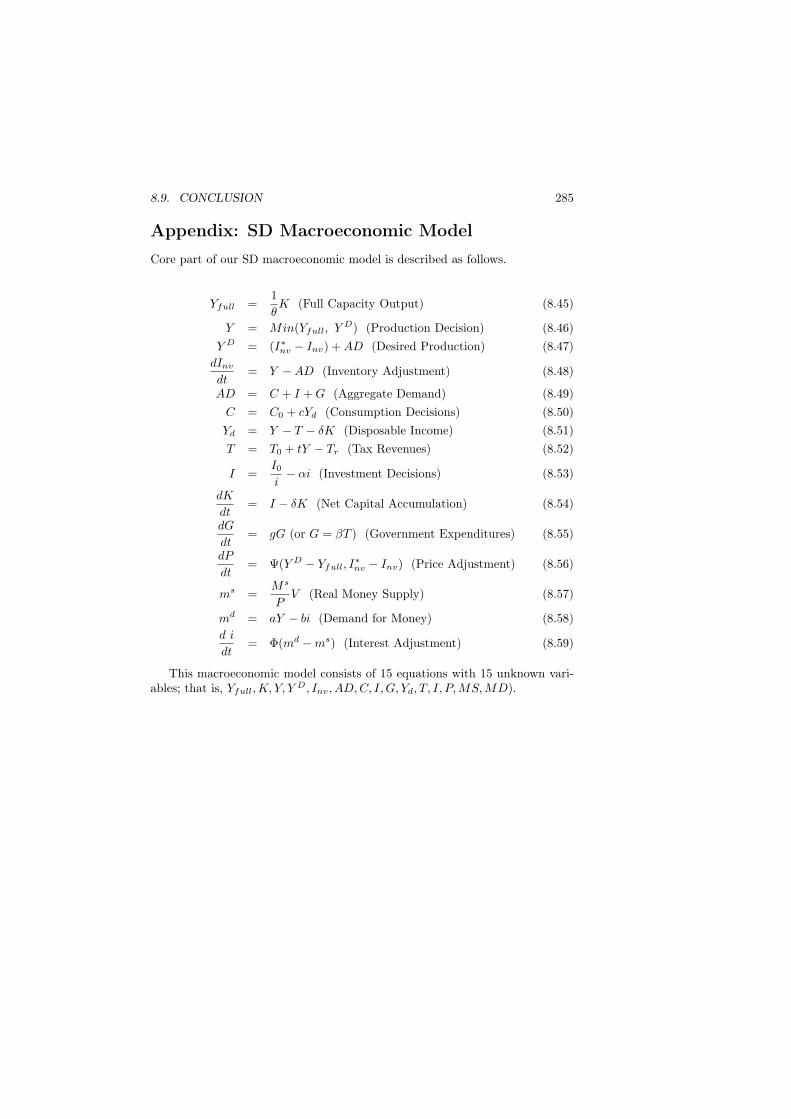
8.9. CONCLUSION 285
Appendix: SD Macroeconomic ModelCore part of our SD macroeconomic model is described as follows.
Yfull =1
θK (Full Capacity Output) (8.45)
Y = Min(Yfull, Y D) (Production Decision) (8.46)Y D = (I∗nv − Inv) +AD (Desired Production) (8.47)
dInvdt
= Y −AD (Inventory Adjustment) (8.48)
AD = C + I +G (Aggregate Demand) (8.49)C = C0 + cYd (Consumption Decisions) (8.50)Yd = Y − T − δK (Disposable Income) (8.51)T = T0 + tY − Tr (Tax Revenues) (8.52)
I =I0i− αi (Investment Decisions) (8.53)
dK
dt= I − δK (Net Capital Accumulation) (8.54)
dG
dt= gG (or G = βT ) (Government Expenditures) (8.55)
dP
dt= Ψ(Y D − Yfull, I
∗nv − Inv) (Price Adjustment) (8.56)
ms =Ms
PV (Real Money Supply) (8.57)
md = aY − bi (Demand for Money) (8.58)d i
dt= Φ(md −ms) (Interest Adjustment) (8.59)
This macroeconomic model consists of 15 equations with 15 unknown vari-ables; that is, Yfull,K, Y, Y D, Inv, AD,C, I,G, Yd, T, I, P,MS,MD).
