Macroinvertebrate Assemblages in Agriculture- and Effluent-dominated Waterways of the Lower Sacramento

River Watershed

Victor de Vlaming1,*, Dan Markiewicz1, Kevin Goding1, Tom Kimball2, and

Robert Holmes3 1Aquatic Toxicology Laboratory, School of Veterinary Medicine: APC, 1321 Haring Hall, University of California, Davis 95616 2Moss Landing Marine Laboratories, 8272 Moss Landing Road, Moss Landing, CA 95039-9647 3California Regional Water Quality Control Board, 11020 Sun Center Drive #200, Rancho Cordova, CA 95670-6114 *To whom questions, comments, and communications should be directed. vldevlaming@ucdavis.edu 530-754-7856

Project funded by:

Surface Water Ambient Monitoring Program (SWAMP) Region 5 – Lower Sacramento River Basin

Fiscal Years: 00/01 and 01/02

Hydrologic Units: 514 (American River), 515 (Marysville), 519 (Valley-American), 520 (Colusa Basin)

i

TABLE OF CONTENTS PageLIST OF FIGURES…………………………………………………………………………. iv LIST OF TABLES…………………………………………………………………………... vii Executive Summary…………………………………………………………………………. viii 1. Introduction……………………………………………………………………………….. 1 2. Methods…………………………………………………………………………………… 5 2.1 Site selection rationale and locations……………………………………………... 5 2.2 Habitat assessments and water quality measurements……………………………. 6 2.3 BMI sampling…………………………………………………………………….. 13 2.4 Sub-sampling and taxonomy……………………………………………………… 14 2.5 Laboratory and field performance evaluation…………………………………….. 14 2.6 Statistical analyses………………………………………………………………... 15 2.6.1 Cluster analysis and ordination…………………………………………... 18 2.6.2 Relationship of BMI metrics to environmental variables………………... 21 2.6.3 Principle components analyses…………………………………………... 21 2.6.4 Relationship between BMI metrics PC1 and environmental variables…... 22 2.6.5 BMI community integrity rankings (biotic index (BI) construction)……. 23 3. Results…………………………………………………………………………………….. 25 3.1 Habitat conditions………………………………………………………………… 26 3.2 Water quality……………………………………………………………………… 26 3.3 BMI community composition…………………………………………………….. 32 3.4 Cluster analyses…………………………………………………………………… 34 3.5 Associations of site taxa clusters with indicator taxa, environmental variables, and BMI metrics……………………………………………………….. 34

ii

TABLE OF CONTENTS continued Page 3.5.1 Taxonomic and environmental differences among high gradient sites….. 39 3.5.2 Taxonomic and environmental differences among low gradient sites ….. 40 3.6 Nonmetric multidimensional scaling (NMS) ordination…………………………. 41 3.6.1 Ordinations of low gradient site taxa data……………………………….. 45 3.6.2 Ordinations of high gradient site taxa data………………………………. 48 3.7 Relationship of BMI metrics to environmental variables………………………… 48 3.8 Metrics principle components analyses (PCA)…………………………………… 52 3.8.1 Associations between metrics PC 1 and environmental variables……….. 56 3.9 Principle components analysis of environmental variables………………………. 56 3.10 Indices of BMI community integrity……………………………………………. 64 3.10.1 Seasonal site comparisons……………………………………………... 68 3.10.2 Summary by watershed/waterway…………………………………….. 83 3.10.2.1 Auburn Ravine ………...……………………………………… 84 3.10.2.2 Butte Creek ………...…………………………………………. 85 3.10.2.3 Dry Creek ………..…………………………………………… 86 3.10.2.4 Coon Creek SMD 1 WWTF ………..………………………… 87 3.10.2.5 Jack Slough ……………………………………………………. 88 3.10.2.6 Main Drainage Canal ………………………………………….. 89 3.10.2.7 Wadsworth Canal ……………………………………………… 92 3.10.2.8 Gilsizer Slough ………………………………………………… 93 3.10.2.9 Pleasant Grove ………………………………………………… 93 4. Discussion………………………………………………………………………………… 94

iii

TABLE OF CONTENTS continued Page 4.1 Waterway gradient………………………………………………………………... 95 4.2 Land use…………………………………………………………………………... 95 4.3 BMI community integrity………………………………………………………… 98 4.3.1 Low gradient waterways…………………………………………………. 98 4.3.2 High gradient waterways………………………………………………… 100 4.4 Physical habitat…………………………………………………………………… 100 4.4.1 Low gradient waterways…………………………………………………. 101 4.4.2 High gradient waterways………………………………………………… 102 4.4.3 Relevant studies………………………………………………………….. 102 4.5 Water Quality……………………………………………………………………... 105 4.5.1 Low gradient waterways…………………………………………………. 106 4.5.2 High gradient waterways………………………………………………… 109 4.5.3 Relevant studies………………………………………………………….. 109 4.6 Identification of stressors…………………………………………………………. 114 4.7 Tolerance values………………………………………………………………….. 116 4.8 Bioassessment data variability……………………………………………………. 116 4.9 Seasonal variation………………………………………………………………… 117 4.10 Taxonomic Effort………………………………………………………………... 119 5. Recommendations………………………………………………………………………… 120 Acknowledgments…………………………………………………………………………… 122 References…………………………………………………………………………………… 123 Appendix A………………………………………………………………………………….. 132

iv

LIST OF FIGURES PageFigure 1. California’s Central Valley, Sacramento and San Joaquin River watersheds, and Delta and San Francisco Bay………………………….…………………………………. 2 Figure 2. Sacramento River watershed………………………………………………………. 7 Figure 3. Sampling sites included in the study of the lower Sacramento River watershed...... 8 Figure 4. Physical habitat scores of low gradient sites in the lower Sacramento River watershed.……………………………………………………………...................................... 27 Figure 5. Physical habitat scores of high gradient sites in the lower Sacramento River watershed.……………………………………………………………...................................... 28 Figure 6. Substrate composition by gradient………………………………………………… 29 Figure 7. Cluster analysis dendrogram of fall samples based on taxonomic similarity……… 35 Figure 8. Cluster analysis dendrogram of spring samples based on taxonomic similarity…... 36 Figure 9. Cluster dendrogram based on taxonomic similarity of fall samples, including indicator taxa, environmental variables, and metrics associated with each cluster.………….. 37 Figure 10. Cluster dendrogram based on taxonomic similarity of spring samples, including indicator taxa, environmental variables, and metrics associated with each cluster.………….. 38 Figure 11. Non-metric multidimensional scaling (NMS) ordination based on taxonomic composition of fall samples, showing environmental variables and metrics highly correlated with differences in BMI communities………………………………………………………... 43 Figure 12. Non-metric multidimensional scaling (NMS) ordination based on taxonomic composition of spring samples, showing environmental variables and metrics highly correlated with differences in BMI communities…………………………………………….. 44 Figure 13. NMS ordination based on taxonomic composition of fall samples collected at low gradient sites, showing environmental variables and metrics highly correlated with differences in BMI communities.…..…………………………………………………………. 46 Figure 14. NMS ordination based on taxonomic composition of spring samples collected at low gradient sites, showing environmental variables and metrics highly correlated with differences in BMI communities.……………………………………………………………... 47 Figure 15. NMS ordination based on taxonomic composition of fall samples collected at high gradient sites, showing environmental variables and metrics highly correlated with differences in BMI communities …………...………………………………………………… 49

v

LIST OF FIGURES continued PageFigure 16. NMS ordination based on taxonomic composition of spring samples collected at high gradient sites, showing environmental variables and metrics highly correlated with differences in BMI communities.…………………………………………………………....... 50 Figure 17. Three-dimensional ordination of BMI metrics data by Principle Components Analysis................................................................................................................ 53 Figure 18. Three-dimensional ordination by Principle Components Analysis of environmental data, including water quality, substrate, nutrients, physical habitat, and land use...................................................................................................................................... 59 Figure 19. (A) Low gradient and (B) high gradient principle components analyses of environmental variables.……………………………………………………………………… 60 Figure 20. Biotic index scores in Auburn Ravine……………………………………………. 71 Figure 21. Biotic index scores in Butte Creek.…………………………………………......... 72 Figure 22. Biotic index scores in Dry Creek.…………………………………….................... 73 Figure 23. Biotic index scores in Coon Creek.………………………………………………. 74 Figure 24. Biotic index scores in Jack Slough.......................................................................... 75 Figure 25. Biotic index scores in Main Drainage Canal …………………………………….. 76 Figure 26. Biotic index scores in Wadsworth Canal.…………………………….................... 77 Figure 27. Biotic index scores in Gilsizer Slough…………………………………………… 78 Figure 28. Biotic index scores in Pleasant Grove………………………………………......... 79 Figure 29. Correlation of riparian zone score with low gradient BI score…………………… 80 Figure 30. Correlation of sediment deposition score with high gradient BI score…………... 81 Figure 31. Mean biotic integrity scores, bracketed by 95% confidence intervals, at sites downstream of 18 January 2001 Main Drain over-spray event………………………. 91

vi

LIST OF TABLES

PageTable 1. Land use surrounding agriculture- and effluent-dominated waterways (ADWs and EDWs) in the lower Sacramento River Watershed……………………………… 9 Table 2. Sampling site locations and seasons sampled during fall 2000 – spring 2002……... 10 Table 3. Description of the metrics of BMI community integrity used in this study………... 17 Table 4. Means and standard deviations of percent fine substrates (mud and sand) and total physical habitat score by site…………………………………………………………………. 30 Table 5. Ranges, mean values (+/- standard deviation), and mean within-site ranges of water-quality variables at agriculture- and effluent-dominated sites in the lower Sacramento River watershed………………………………………………………………….. 31 Table 6. Most common taxa in low gradient and high gradient waterways………………..... 33 Table 7. Environmental variables included in the final linear models of MANOVA analyses using all BMI metrics as response variables. Three multiple regression models were constructed: one for the entire dataset, one for the low gradient sites, and one for the high gradient sites…………………………………………………………………………….. 51 Table 8. Loadings of BMI metrics onto the first three principle components of full data set PCA analyses……………………………………………………………………………… 54 Table 9. Loadings of BMI metrics onto the first three principle components of the low- and the high-gradient PCA analyses.…………………………………………………………. 55 Table 10. Environmental variables significantly associated with BMI metrics Principle Component 1 in final multiple regression models. Three multiple regression models were constructed: one for the entire dataset, one for the low gradient sites, and one for the high gradient sites………………………………………………………………………………….. 57 Table 11. Loadings of environmental variables onto the first three principle components of the full dataset PCA analysis………………………………………………………………. 61 Table 12. Loadings of environmental variables onto the first three principle components of the low and high gradient PCA analyses………………………………………………….. 62 Table 13. Pair-wise correlations of BMI metrics with PC1 of environmental parameter PCAs of the entire dataset, low-, and high-gradient site data subsets………………………… 63

vii

LIST OF TABLES continued PageTable 14. BMI metrics included in the Biotic Indices created to discriminate more impacted sites from less impacted sites.……………………………………………………… 65 Table 15. Signal to noise (S/N) ratios of BMI metrics chosen for the low gradient and high gradient Biotic Indices, and Pearson product-moment correlations between these metrics and five environmental variables possibly indicating anthropogenic stress………………….. 66 Table 16. Mean biotic index scores of fall and spring samples at low gradient sites, including 95% confidence intervals…………………………………………………………... 69 Table 17. Mean biotic index scores of fall and spring samples at high gradient sites, including 95% confidence intervals…………………………………………………………... 70 Table 18. BMI metrics included in season- and gradient-specific biotic indices created to discriminate more impacted sites from less impacted sites.……………………………...... 82

viii

Executive Summary

A large area of the Central Valley is characterized by irrigation-subsidized agriculture and water

development projects. The natural flow regimes and physical aquatic habitats of most Central

Valley waterways are significantly altered and/or modified due to current and historical practices

(including mining, colonization/urbanization, and agriculture). Thousands of miles of canals

have been constructed, and most natural channels have been altered and/or modified to move

stored water from foothill and mountain reservoirs to water users throughout the valley, and

state. Currently, the vast infrastructure of Central Valley waterways remain heavily managed to

support current societal needs including irrigation of agricultural lands, municipal and industrial

demands, and water quality/supply needs.

The Central Valley Regional Water Quality Control Board (CVRWQCB), is responsible for

protecting beneficial uses of surface waters, and has relied on toxicity testing for monitoring and

assessment of aquatic contaminants and aquatic life toxicity to determine compliance with water

quality objectives in their Basin Plan. In 2000 the CVRWQCB funded an exploratory project

with the University of California, Davis Aquatic Toxicology Laboratory that applied benthic

macroinvertebrate (BMI) bioassessment to agriculture- (ADWs) and effluent-dominated

waterways (EDWs) of the lower Sacramento River Watershed. BMIs constitute an important link

in freshwater aquatic ecosystem structure (food web). BMI community integrity and health vary

in response to a variety of stressors that affect physical habitat and water quality. Bioassessments

provide indications of aquatic system ‘biotic integrity’ as well as physical habitat condition.

BMIs are considered effective indicators of aquatic system ecological health.

ix

The goal of this study was to explore the utility of the BMI bioassessment approach in assessing

condition of two types of regionally important waterways, Central Valley ADWs and EDWs.

Very little is known regarding biological condition in ADWs and EDWs. Objectives of this

study included: 1) examine the physical habitat and water quality parameters that potentially

determine BMI community integrity; 2) probe the nature and variability of BMI communities in

ADWs and EDWs; 3) search for strong associations between biological communities and

environmental parameters using a variety of statistical approaches; and 4) establish a baseline of

BMI community composition and habitat conditions from which future assessments may be

compared.

ADWs occur in the valley floor, and can be natural, modified natural, and/or constructed

waterways. Aquatic life community integrity can be impacted in ADWs by physical habitat

destruction or modification, hydrology regimes (e.g., modified and intermittent flow), sediment,

elevated nutrients, contaminants (including organic chemicals, such as pesticides and other

agricultural chemicals and inorganic chemicals) and organic wastes. EDWs are characterized as

waterways that, due to low or intermittent flow, may consist of a majority of flow originating

from discharged effluents. EDWs are common in the Central Valley foothills, where natural

stream flows typically diminish during dry periods of summer and fall. Physical habitat

destruction or modification, effluent contaminants, and contaminants in urban runoff likely

impact biological communities in EDWs.

The two-year bioassessment investigation began fall 2000 and continued through spring 2002.

Fall and spring BMI samples were collected from ADWs (Butte Creek, Gilsizer Slough, Jack

x

Slough, Main Drainage Canal, Wadsworth Canal) and EDWs (Auburn Ravine, Dry Creek,

Pleasant Grove Creek) at a range of sites within each watershed. Most of the ADW sites were

low gradient (slope <0.2) occurring within the valley floor. Most EDW sites occurred in the

Sierra Nevada foothills northeast of the City of Sacramento and were mostly high gradient

(containing riffles). Low and high gradient versions of the California Stream Bioassessment

Protocol (CSBP) were used to guide collection of macroinvertebrates. Simultaneously, physical

habitat and land use data were collected. Traditional water quality data were gathered monthly at

the same sites during the two-year period of macroinvertebrate collection.

Bioassessments provided an indication of BMI community integrity in ADWs and EDWs of

lower Sacramento River watershed. In general, the most severely impacted sites were located

adjacent to the highest intensities of agricultural and urban land uses. At three of four municipal

treatment facilities, BMI community integrity below the discharge was not significantly different

compared to upstream community integrity. Seasonal differences (within site variability) were

detected in BMI community integrity in ADWs and EDWs. These differences may be related to

natural temporal variation, to seasonal influences of anthropogenic factors, or both.

The largest differences in BMI taxa composition in this investigation were between high and low

gradient sites. A range of BMI community integrity was observed within each waterway low and

high gradient site groups. Downstream sites on ADWs tended to manifest more robust BMI

communities than upstream sites surrounded by agricultural land use. EDWs were characterized

by more robust BMI communities at sites farther away from urban areas compared to sites within

xi

urban areas. Environmental parameters likely to be determinants of BMI community integrity

included substrate, several physical habitat parameters, and some water quality variables.

Although reports that describe reference metrics/conditions (determined at sites un-impacted or

‘least disturbed’ by human activities) for BMI community integrity have not been published for a

majority of Central Valley waterways, comparisons among sites of similar gradient allowed

assessment of relative range and ranking of community integrity. ADWs manifested a range of

biological conditions suggesting that they could support more robust BMI community integrity if

physical habitat and water quality were not degraded. Likewise, EDWs were characterized by a

range of BMI community integrity conditions. Detrimental effects on BMI community integrity

consequent to urban land used were evident in foothill streams.

Habitat variables including decreased riparian zone, increased channel alteration, and increased

sedimentation, and loss of high quality benthic habitat were discovered as probable determinants

of BMI community integrity. Of the environmental parameters measured, water quality

parameters appeared to exert less effect on BMI community integrity than physical habitat

factors. We hypothesize that effects of water quality variables were difficult to detect with the

bioassessment procedure because physical habitat conditions were so poor at most sites,

especially in ADWs. Bioassessment provided an indication of biotic integrity in ADWs and

EDWs, but bioassessment alone is not capable of definitively identifying the stressors causes

impacts. Compromised BMI community integrity and poor aquatic habitat conditions were

identified in many ADWs and EDWs of the lower Sacramento River watershed.

xii

Results of this study clearly reveal that BMI communities integrate ‘cumulative’ effects of

various land uses and associated stressors, including physical habitat and water quality

conditions. Partitioning the effects of various stressors on BMI communities and identification of

those stressors will require carefully designed studies. Assessing habitat conditions with BMI

bioassessment protocols is likely to be straightforward, while assessing water quality

impairments may pose more of a challenge in waterways with poor physical habitat conditions.

Contaminants and identification of aquatic life toxicity in surface waters can be measured

directly by chemical analyses and toxicity testing. An understanding of strengths and limitations

of methods will be important in designing monitoring projects. Bioassessment information can

be an important component of comprehensive evaluations of aquatic ecosystem condition when

used in concert with water and sediment chemistry and toxicity data (e.g., triad approach).

This report provides basic background and baseline information, which will be valuable the

design of future bioassessment projects. Section 5 (see page 120) of this report offers 12

recommendations intended to refine, enhance, and focus future bioassessments and data

analyses. Also included are bioassessments issues to be addressed. This project was funded

through the Surface Water Ambient Monitoring Program (SWAMP) from the lower Sacramento

River Basin of Region 5 SWAMP fund allocation.

1

1. Introduction In the Central Valley of California the Sacramento River and San Joaquin River converge

to form the Sacramento-San Joaquin Delta before flowing into San Francisco Bay (Fig.

1). The Sacramento River serves as a catchment for waters draining the entire northern

portion of the Central Valley and drains approximately 70,000 km2. Omernik (1987)

designated the Sacramento River and San Joaquin River contiguous basins as the Central

Valley ecoregion. This ecoregion is characterized by irrigation-subsidized agriculture,

and water development activities have significantly modified stream flow regimes. All

large rivers and most small streams are dammed for flood control and runoff storage.

Stored water is transported through natural channels or constructed canals for irrigation

of agricultural lands, municipal and industrial needs, and to fulfill environmental

requirements. Annual precipitation in the Sacramento River basin averages 36 to 63 cm.

This rainfall occurs primarily in the November through February period. The

predominant landscape feature of the Sacramento River basin is agriculture (Domagalski

et al., 1998; Groneberg et al., 1998). Urban land use and historical mining activities are

also important influences in the basin. All of these activities and modifications in the

Central Valley have resulted in widespread alteration of riparian zones, waterway

geomorphology, flow, and water quality raising concerns about the health of the region’s

aquatic ecosystems.

Agriculture-dominated waterways (ADWs) receive greater than fifty percent of flow

from irrigation runoff. Irrigation occurs primarily during the dry season (March through

September). ADWs can be natural streams, constructed waterways, or a combination of

both. There are over 9,173 km of natural and constructed ADWs in the Sacramento River

watershed; natural ADWs constitute approximately 10 percent of the total. A wide range

of physical and biological conditions exist in both natural and constructed agricultural

drains. Waterways in which, due to low or intermittent flow, a majority of the flow is

constituted by discharged effluent are designated as effluent-dominated waterways

(EDWs). These waterways are common near areas of extensive urban development, and

are a focus of concern because of possible water quality effects of the combination of

effluent and urban runoff that they receive.

2

Fig. 1. California’s Central Valley, Sacramento and San Joaquin River watersheds, and Delta and San Francisco Bay.

3

Due to the seasonality of rain and snowmelt, most wadeable (< 1.5 meters depth) streams

and creeks in the Sacramento River watershed are intermittent unless supplemented by

irrigation water, urban runoff, and/or discharge of treated effluent. Many streams, creeks,

and rivers within the Sacramento River watershed are dominated either by water that will

be used for irrigation or by irrigation runoff (ISWP, 1991). The agriculture-dominated

segments of most waterways usually occur in the lower valley floor (< 165 m elevation).

The largest urban area in the Sacramento River basin is the City of Sacramento with a

population of over a million. Placer County, north of Sacramento, has experienced

population growth ranking among the highest in Northern California for several years.

Most population growth in Placer County has occurred in the valley floor region of the

county, expanding the cities of Roseville and Lincoln. The rapid population growth

resulted in a net loss of irrigated agricultural land in the Sacramento River basin (CDWR,

1998).

Population growth over the next fifty years is expected to add another 1.7 million people

in western Placer County. Numerous municipal wastewater treatment plants are being

constructed to handle the large regional population growth. Many of these wastewater

treatment facilities, both planned and existing, will discharge to low flow or intermittent

Placer County EDWs. The low-flow intermittent nature of EDWs raises concern of

possible aquatic community disturbance because there is little or no stream dilution of

wastewater discharges.

Water column chemistry and aquatic species toxicity studies in ADWs of the Central

Valley ecoregion documented impaired water quality conditions (e.g., Domagalski, 1996;

de Vlaming et al., 2000; Holmes and de Vlaming, 2003). Pesticides (including

herbicides, insecticides, fungicides) totaling millions of kilograms are applied annually in

Sacramento River basin (CDPR, 2003). Much of the toxicity to aquatic species in ADWs

has been linked to insecticides (e.g., de Vlaming et al., 2000). Ambient water toxicity

testing and chemistry measurements conducted by National Pollutant Discharge

4

Elimination System (NPDES) dischargers have also indicated periodic water quality

degradation in EDWs.

Bioassessments are a component of assessing the health and integrity of aquatic

communities in several areas of the United States. These procedures have served as

important tools for evaluating impacts from anthropogenic disturbances such as non-point

source pollution and alterations of stream channels, riparian areas, and entire stream

catchments (Fore et al., 1996; U.S. EPA, 2002). Benthic macroinvertebrate (BMI)

communities are a critical component of stream ecosystems. Although there is

considerable concern regarding health and integrity of biotic communities, few BMI

community studies have been conducted on waterways in California’s Central Valley.

Leland and Fend (1998) conducted artificial-substrate macroinvertebrate bioassessments

in the lower San Joaquin River and associated tributaries applying a multivariate analysis

approach, but did not sample in the Sacramento River Basin. Brown and May (2000)

conducted biological assessments (1993-97) on the lower Sacramento and San Joaquin

River drainages as a component of the U.S. Geological Surveys (USGS) National Water

Quality Assessment Program. The focus of the study was on snag macroinvertebrate

assemblages, with sampling according to Meador et al. (1993). Hall and Killen (2001)

applied California Department of Fish and Game (Harrington, 1999) BMI procedures to

assess benthic communities and habitat in a representative urban and agricultural

waterway in the Central Valley. Applying the U.S. EPA Environmental Monitoring and

Assessment Program (EMAP) procedure (Lazorchak et al., 1998), relationships between

environmental gradients and macroinvertebrate assemblages in lotic habitats of the

California Central Valley were examined by Griffith et al. (2003).

A primary goal of this study was to assess BMI community structure and physical stream

habitat conditions in several ADWs and EDWs of the lower Sacramento River watershed.

These regionally prominent aquatic ecosystems, including BMI communities, are poorly

understood. A second objective was to establish a baseline of BMI community

composition and habitat conditions from which future assessments may be compared.

5

Another intent was to identify environmental factors that potentially impact BMI

assemblages, although limited resources precluded evaluation of all potential stressors on

aquatic ecosystem biota. As stated, these types of waterways are characterized by highly

modified, or unnatural, conditions. Another aim of this study was to examine the nature

of variability among aquatic communities, physical habitat and water quality parameters

in ADWs and EDWs. At the time of this investigation no reference metrics/conditions

for Central Valley waterways were published for gauging relative BMI community

integrity/health. Therefore, while it was impossible to determine the extent of biological

impairment at the sites examined, we sought to measure the health of the BMI

communities at these sites relative to one another.

2. Methods

2.1 Site selection rationale and locations Sampling sites were in agriculture- and effluent-dominated tributaries to the lower

Sacramento River (Figs. 2 and 3). Five ADWs (Butte Creek, Jack Slough, Gilsizer

Slough, Main Drainage Canal, and Wadsworth Canal) and three EDWs (Auburn Ravine,

Dry Creek, and Pleasant Grove Creek) were selected for sampling. Multiple sites were

selected on each waterway for more complete characterization and to allow examination

of possible impacts related to various land use practices. The basic rationale for

waterway selection for ADWs was based upon historical and current toxicity and

chemistry data for each waterway – although it was not our intent to evaluate the

relationships between bioassessment and other monitoring data from other time periods

and other special studies. Preference was given to ADWs that had such existing

information available. Sites were generally selected in ADWs to reflect a gradient of

agricultural land use and allow for possible examination and partitioning of different

cropping patterns and intensity of those patterns within each watershed. EDWs were

selected either because there were wastewater treatment plants in operation on such

waterways or there are planned treatment plants. EDWs that had watershed groups

working in those waterways were preferred as this allowed for coordination of

monitoring and access to private property. In general, sampling sites in EDWs were

6

selected to reflect a gradient of urban land use within each watershed, and to bracket

wastewater treatment plant effluent discharges. Access to sampling sites from road

crossings was also a factor in site selection for all sites.

Land uses surrounding waterways included in this investigation are summarized in Table

1. Land use was calculated based on GIS layers and delimited by watershed boundary.

Many agriculture-dominated watersheds were unnatural with boundaries identified from

irrigation district historical records. Most ADWs consist of 70 percent or more

agricultural land use. Urban land use in the EDWs ranged between 9 to 47 percent. Dry

Creek and Pleasant Grove Creek EDWs consist of 30 percent or greater of agricultural

land use in the downstream-most portions of each basin. Because natural vegetation

predominates Butte Creek and Auburn Ravine, these sites were projected to manifest

higher biological and habitat conditions. Native vegetation is a classification consisting of

grasses, brush, timber, and forests (CDWR, 1993). Sampling site locations within each

watershed are summarized in Table 2. Habitat assessments were conducted

simultaneously with BMI collections. Most sites were sampled during spring and fall

(2000/01; 2001/02) over the two-year study period.

2.2 Habitat assessments and water quality measurements Habitat structure is one of five parameters (habitat structure, flow regime, water quality,

energy source, and biotic interactions) that human activities can alter that, in turn,

degrade water resources and impact BMI community health and integrity (Karr and Chu,

1999). For a more comprehensive understanding of spatial variations in BMI community

structure/integrity and potential causes of biotic disturbances, habitat assessments were

conducted simultaneously with BMI collections.

Physical habitat assessments were conducted at each site. These included two

components: (1) the CSBP Worksheet that focuses on water quality and habitat

parameters at the individual riffle/transect level and (2) the US EPA nationally

standardized Habitat Assessment Field Data Sheet (Barbour et al., 1999) that targets

7

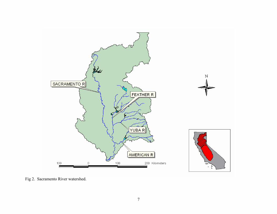
Fig 2. Sacramento River watershed.

8

Fig. 3. Sampling sites included in the study of the lower Sacramento River watershed. The main waterbodies sampled included Butte Creek (BC), Main Drainage Canal (MD), Wadsworth Canal (WC), Jack Slough (JS), Gilsizer Slough (GS), Auburn Ravine (AR), Dry Creek (DC), and Pleasant Grove Creek (PG), as well as sites bracketing the SMD1 waste water treatment facility (WW).

BC3

BC2

BC1

WC1

MD2 MD1

MD3

MD4

MD9

MD6

MD5

WC2

WC3

WC4

WC5

WC6 JS1

JS2 JS3

GS1 WW1, WW2, WW3

AR2 AR3 AR4 AR5-6

AR7

DC2 DC3 DC4

DC5 DC6

DC10 DC11

DC8-9

PG1 PG2 PG3

PG5

DC12-13

9

Table 1 Land use surrounding low gradient and high gradient waterways in the lower Sacramento River Watershed Low Gradient High Gradient Pleasant

Grove Ck. Jack Sl. Wadsworth

Canal Main Canal Gilsizer Sl. Butte Ck. Auburn

Ravine Dry Ck.

Agriculture 34% 72% 69% 78% 69% 21% 29% 9% Urban 14% 3% 4% 4% 28% 6% 9% 47% Native Vegetation

52% 25% 27% 18% 3% 73% 62% 44%

Total Acres 44,870 40,441 74,178 32,588 31,096 134,583 51,170 74,069

10

Table 2 Sampling site locations and seasons sampled during fall 2000 – spring 2002

Sampling Season Waterbody Sites Location Latitude Longitude Fall Spring Auburn Ravine AR2 Moore Rd. 38.8700 121.3566 00, 01 01,02

AR3 Hwy 65 38.8885 121.2850 00, 01 01,02 AR4 Fowler Rd. 38.9011 121.2125 00, 01 01,02 AR5 Downstream Auburn WWTF 38.8897 121.1123 00, 01 01,02 AR6 Upstream Auburn WWTF 38.8891 121.1097 00, 01 01,02 AR7 Palm Avenue - Most Upstream 38.9064 121.0751 00, 01 01,02

Dry Creek DC2 Dry Creek - Cook Riolo Rd. 38.7368 121.3383 00, 01 01,02 DC3 Dry Creek - Atkinson Rd. 38.7343 121.3087 00, 01 01,02 DC4 Antelope Creek - Sunset Blvd. 38.7876 121.2489 00, 01 01,02 DC5 Antelope Creek - Taylor Park 38.8183 121.2164 00, 01 01,02 DC6 Secret Ravine - Loomis Park 38.8245 121.1755 00, 01 01,02 DC8 Miners Ravine - d/s SMD3 WWTF 38.7968 121.1358 01,02 DC9 Miners Ravine - u/s SMD3 WWTF 38.7982 121.1352 01,02 DC10 Linda Creek - Champion Oaks

Blvd. 38.7300 121.2493 00, 01 01,02

DC11 Miners Ravine - Auburn Folsom Blvd.

38.7545 121.1702 00, 01 01,02

DC12 Dry Creek - d/s Roseville WWTF 38.7343 121.3246 00, 01 DC13 Dry Creek - u/s Roseville WWTF 38.7339 121.3187 00, 01

Coon Creek WW1 Coon Creek - u/s SMD1 WWTF 38.9663 121.1096 00, 01 01,02 WW2 Coon Creek - d/s SMD1 WWTF 38.9657 121.1130 01,02 WW3 Rock Creek - u/s SMD1 WWTF 38.9643 121.1101 01,02

Pleasant Grove Ck. PG1 Pleasant Grove Creek - Pettigrew Rd.

38.8124 121.4245 00, 01 01,02

PG2 Pleasant Grove Creek - Fiddyment Rd.

38.7959 121.3555 00, 01 01,02

PG3 Pleasant Grove Creek - Industrial Blvd.

38.8055 121.3087 00, 01 01,02

PG5 South Branch PGC - Pleasant Gr. Blvd.

38.7711 121.3159 00, 01 01,02

Butte Creek BC1 Butte Creek - Aguas Frias Rd. 39.5301 121.8584 00, 01 01,02 BC2 Butte Creek - Durham/Dayton

HWY 39.6471 121.7870 00, 01 01,02

BC3 Butte Creek - HWY 99 39.6994 121.7771 00, 01 01,02 Gilsizer Slough GS1 Gilsizer Slough - O'Banion Rd. 39.0260 121.6592 00, 01 01,02 Jack Slough JS1 Jack Slough - Doc Adams Rd. 39.1623 121.5959 00, 01 01,02

JS2 Jack Slough - Woodruff Rd. 39.2149 121.5513 00, 01 01,02 JS3 Jack Slough - Loma Rica Rd. 39.2253 121.5116 00, 01 01,02

Main Drainage Canal MD1 Main Canal - Farris Rd 39.3747 121.7828 00, 01 01,02 MD2 Main Canal - Farris Rd. North

Lateral 39.3996 121.7562 00, 01 01,02

MD3 Main Canal - South Ave. Lateral E 39.3924 121.6840 00, 01 01,02 MD4 Main Canal - West Biggs/Gridley

HWY Lateral H 39.3952 121.7160 00, 01 01,02

MD5 Main Canal - Ord Ranch Rd. Lateral E-7

39.3804 121.6787 00, 01 01,02

MD6 Main Canal - West Biggs/Gridley HWY Lateral E-7

39.3779 121.7062 00, 01 01,02

continued

11

Sampling Season Waterbody Sites Location Latitude Longitude Fall Spring Main Drainage Canal MD9 Main Drain - Phil Fran Dr. 39.4359 121.6789 01,02 Wadsworth Canal WC1 Wadsworth Canal - Butte House

Rd. 39.1710 121.7165 00, 01 01,02

WC2 Wadsworth Canal - Nuestro Rd. RD777 Lateral

39.1854 121.6950 00, 01 01,02

WC3 Wadsworth Canal - Paseo Ave. RD777 Lateral

39.2498 121.6789 00, 01 01,02

WC4 Wadsworth Canal - Eager/Larkin Rd. Lateral

39.1897 121.6620 00, 01 01,02

WC5 Live Oak Slough - Clark Rd. 39.2331 121.6653 00, 01 01,02 WC6 Wadsworth Canal - Franklin Rd. 39.1273 121.7566 00, 01 01,02

Table 2 continued

12

habitat conditions along the entire reach. Each of these physical habitat assessments has

a low and high gradient version. Riffle/transect data collected included depth, velocity,

and substrate composition. At each transect, these measurements were recorded as the

mean of three measurements. Substrate composition was recorded as an observational

estimate of percentages of mud (<0.2 cm), sand (<0.2 cm), gravel (0.2 to 5.0 cm), cobble

(5.0 to 25.0 cm), boulder (>25.0 cm), and bedrock/hardpan (solid rock or clay forming a

continuous surface). Substrate consolidation was determined to be either ‘loose’,

‘moderate’, or ‘tight’.

Site habitat data included estimates of ten physical habitat parameters (epifaunal

substrate, sediment deposition, channel sinuosity, riparian vegetative zone width, pool

substrate, available cover, channel flow status, bank stability, pool variability, channel

alteration, and vegetative protection). Each habitat parameter consists of ‘poor’,

‘marginal’, ‘sub-optimal’, and ‘optimal’ scoring categories. Each habitat parameter is

scored using semi-qualitative criteria (Barbour et al., 1999). For analyses involving the

combined high and low gradient datasets, the high gradient embeddedness, velocity/depth

regime, and frequency of riffles scores were considered to be equivalent to the low

gradient pool substrate, pool variability, and channel sinuosity measures.

Water quality parameters were recorded monthly at each site and at the times of BMI

collection, except the following sites, where these measurements were taken only at the

times of BMI collection: MD9, WC6, DC8, DC9, DC12, DC13, WW1, WW2, WW3. At

the times of BMI collection, water quality measurements were recorded prior to

collection of BMIs at the second riffle/transect (CDFG, 2003). Measurements included

pH, specific conductance (SpC), dissolved oxygen (DO), and temperature. Turbidity,

ammonia, hardness, and alkalinity measurements were performed on monthly water

samples from each site, except AR5, AR6, and the sites listed above, where these

measurements were not taken. Orthophosphate and nitrate-nitrogen nutrient analyses

were conducted during fall 2001 using a HACH DR890 Colorimeter at all sites except

those listed above.

13

Canopy cover was estimated with a hand held densiometer. At high gradient (slope >

0.2) sites, gradient was measured using a stadia rod and a clinometer. GPS coordinates

were recorded at the second riffle/transect of all sites.

2.3 BMI sampling BMI bioassessments were performed according to the California Stream Bioassessment

Procedure (CSBP; Harrington, 1999). The CSBP is a California adaptation of the US

EPA Rapid Bioassessment Protocol (Barbour et al., 1999) and focuses on richest stream

habitat (generally riffles). Many of the streams, especially the ADWs, sampled were low

gradient with no riffle habitat; substrate was primarily mud and fine grains. The non-

riffle, low gradient (slope < 0.2) sites were sampled with a modified version of the CSBP

(CDFG, 2003) for low gradient waterways.

Sampling riffle habitat consisted of identifying five riffles in a stream reach, then

randomly selecting three of the five to sample. If only three riffles could be identified

within the reach (<600 meters), those riffles were sampled. The distance between the

first and last riffle determined reach length, and generally was less than 100 meters.

Beginning at the most downstream area, sampling occurred across a transect in the top

third of the riffle. Transects were chosen at random from all possible meter marks

available in the upper third of the riffle. A 500 um mesh D-frame kick net was placed

immediately downstream of the transect, and a 0.3 X 0.6 meter of substrate upstream of

the net was disturbed. Disturbing the stream bottom included kicking, turning over and

scrubbing of all large debris (cobble, wood chunks, gravel, leaves). A total of three, 0.3

X 0.6 meter areas, were sampled across each transect, composited into a sample

container, and preserved with 95 percent ethanol. This process was repeated at the

remaining two upstream riffles.

Sampling low gradient, fine substrate-dominated streams using a modified low gradient

CSBP sampling adaptation required identification of 100 meter standardized reach

lengths at each site. Three randomly-selected, meter mark transects were chosen for

sampling within the 100 meter reach. Three, 0.3 X 0.6 meter, areas were sampled with

14

kick net across each transect as described above. The three collection areas usually were

bank margins and the thalweg (deepest point of stream cross section). The three, 0.3 X

0.6 meter transect samples were composited. Gradient (percent slope) was determined as

the change in elevation between upstream and downstream ends of a sampling reach.

2.4 Sub-sampling and taxonomy In the laboratory, three hundred organisms were sub-sampled and removed from each

transect composited sample for taxonomic identification, metric analyses, and abundance

estimations. Sub-sampling consisted of: (1) transferring each sample to a 500 um sieve,

gently rinsing to flush out fine particles, (2) removing large debris such as gravel, fresh

leaves, and sticks after thoroughly inspecting for entangled BMIs, (3) submerging the

sieve containing BMI’s in a 2.5 liter container of water to homogenize the sample, (4)

draining the sieve, and (5) inverting the sieve over a white tray with numbered grid lines.

Samples were spread evenly over 5X5 cm grids so as to accommodate the entire sample

volume. Grids to be examined by dissecting microscope were selected at random. BMIs

were removed from grids and transferred to a vial containing 70% ethanol (EtOH) until a

300 count was achieved. The last grid examined to achieve the three hundred count was

completely processed, with additional BMIs placed into an ‘extras’ vial. BMIs from the

‘extra’ vial are necessary for an accurate estimate of sample BMI abundance. Sample

abundance was estimated as the total number of BMIs removed from a sample, divided

by number of grids processed, multiplied by total number of grids covered by the sample.

Most BMIs were identified to genus level. However, midges (Chironomidae) were

identified to tribe, worms (oligochaetes) to family, and clams (bivalves) as well as

crayfish (Decapoda) to superfamily. Our criterion for this study: at least 285, but no

more than 315 BMIs were to be recovered from each sample.

2.5 Laboratory and field performance evaluation To assure that data generated were of high quality and credible, performance evaluation

(quality assurance) measures were included in this study. Both internal (University of

California, Davis Aquatic Toxicology Laboratory; UCD ATL) and external performance

15

evaluations on taxonomic identification were a component of this study. Internal

evaluation consisted of re-identification by a second taxonomist of BMIs randomly

selected 10 percent of all samples. External performance evaluation was performed by

the CDFG Bioassessment Laboratory, Rancho Cordova, CA on 20 percent of all year one

(fall 2000, spring 2001) samples, and by Bioassessment Services Inc. (Folsom, CA) on

10 percent of all study year two (fall and spring) samples. A total of 56 samples were

evaluated. There were no major discrepancies between UCD ATL identifications and

those of CDFG (misidentifications in only 4 percent of 1,018 taxa vials) or

Bioassessment Services, Inc. (misidentification in only 1.7 percent of 177 taxa vials.

These performance evaluations lend credibility to the taxonomic identification presented

herein.

Prior to actual sampling, field crews engaged in trial runs to assure consistency of

sampling efforts and habitat scoring. During actual sampling events habitat scoring was

completed individually by two field crew members at 20 percent of the sites. These

individual scorings were compared and, if necessary, adjusted to achieve agreement.

There was 95 to 100 percent agreement in individual scoring of habitat parameters at all

sites.

For sub-sampling, only UCD ATL internal performance evaluation was conducted. Ten

percent of all samples were subjected to re-evaluation. Our sub-sampling criterion for

this investigation was that no more than ten percent of the BMIs in a sample could be

overlooked. No remnant samples exceeded the ten percent criterion; in a majority of

samples less than five percent of BMIs were overlooked.

2.6 Statistical analyses Multivariate and multimetric analyses were applied to investigate spatial and temporal

variability in BMI communities. Relationships between community structure, a range of

environmental variables describing habitat and water quality, and a number of widely

used metrics indicative of BMI community integrity also were examined. Metrics of

BMI community integrity used in this study are described in Table 3.

16

In many cases, we found it informative to analyze data from high gradient waterways

separately from data from low gradient waterways (low gradient = slope < 0.2, high

gradient = slope > 0.2). This decision was supported by a cluster analysis which clearly

separated the waterways by gradient (see Fig. 7). Note that the most downstream sites in

two of the high gradient waterways were actually low gradient (AR2 and BC1), but these

sites were analyzed in the high gradient dataset because of their placement on the cluster

dendrogram.

Where data conformed to assumptions of normality and homogeneity of variance,

parametric statistics were performed, otherwise nonparametric equivalents were used.

The significance of multiple simultaneous tests was evaluated after sequential Bonferroni

correction, which adjusts the tests to be less likely to indicate a significant difference

where one does not exist. The composition and range of BMI communities were probed

by cluster analysis, indicator species analysis, and nonmetric multidimensional scaling

(NMS) ordination. Analysis of variance (ANOVA) was applied to distinguish the

environmental variables and BMI metrics associated with the site groups (based on taxa

similarities) identified by cluster analysis. Principal Component Analyses (PCAs) and

multivariate linear models were applied to identify environmental variables accounting

for most of the variability in BMI metrics at both high and low gradient sites. In a

complimentary analysis, we conducted a Multiple Analysis of Variance (MANOVA) and

developed a linear model to examine the statistical significance of relationships between

BMI metrics and environmental variables. Transect data points were treated as replicates

of their reach in analyses examining within reach versus between reach variability. For

analyses which did not consider within reach, within event variability, a single data point

for each site was calculated by taking the average of the measurements taken at the three

transects.

17

Table 3 Description of the metrics of BMI community integrity used in this study Metric Description Taxonomic Richness • Number of taxa present Shannon Diversity Index • Measure of taxonomic diversity considering the number of

taxa present and the relative abundances of all taxa EPT Taxa • Number of taxa present of the insect orders Ephemeroptera,

Plecoptera, and Trichoptera EPT Index • Percentage of BMIs belonging to the EPT orders Sensitive EPT Index • Percentage of BMIs which belong to the EPT orders and with

pollution tolerance (Hilsenhoff) scores not exceeding four ETO Taxa • Number of taxa present of the insect orders Ephemeroptera,

Plecoptera, and Odonata ETO Index • Percentage of BMIs belonging to the ETO orders Ephemeroptera Taxa • Number of mayfly taxa present Plecoptera Taxa • Number of stonefly taxa present Trichoptera Taxa • Number of caddisfly taxa present Odonata Taxa • Number of damselfly and dragonfly taxa present Tolerance Value • Average pollution tolerance (Hilsenhoff Biotic Index) of the

BMIs present (Range: 1 – 10) % Intolerant • Percentage of BMIs with pollution tolerance (Hilsenhoff)

scores not exceeding four % Tolerant • Percentage of BMIs with pollution tolerance scores exceeding

five % Dominant Taxon • Percentage of BMIs belonging to the most abundant taxon % Hydropsychidae • Percentage of BMIs belonging to the somewhat pollution

tolerant Hydropsychidae taxa (Trichoptera) % Baetidae • Percentage of BMIs belonging to the somewhat pollution

tolerant Baetidae taxa (Ephemeroptera) % Chironomidae • Percentage of BMIs belonging to the pollution tolerant

Chironomidae taxa (Diptera) % Tanytarsini / % Chironomini

• The ratio of the proportional abundances of the chironomid tribes Tanytarsini (somewhat tolerant of low DO) and Chironomini (highly tolerant of low DO)

% Insects • Percentage of BMIs belonging to insect taxa % Oligochaeta • Percentage of BMIs belonging to highly pollution tolerant

worm taxa % Collectors • Percentage of BMIs in the collector feeding group % Filterers • Percentage of BMIs in the filterer feeding group % Filterers + Collectors • Percentage of BMIs in the collector or filterer feeding groups % Grazers • Percentage of BMIs in the grazer feeding group % Predators • Percentage of BMIs in the predator feeding group % Shredders • Percentage of BMIs in the shredder feeding group % Semivoltine • Percentage of BMIs taking longer than one year to reach

reproductive maturity % Multivoltine • Percentage of BMIs having more than one complete generation

every year

18

2.6.1 Cluster analysis and ordination

Taxa composition was probed using hierarchical cluster analysis, indicator species

analysis, and ordination by NMS to reveal the strongest patterns in BMI community

structure across sites. Hierarchical cluster analysis lumped sites into groups based on

similarity in BMI communities. Indicator species analysis (Dufrêne and Legendre, 1997)

revealed the taxa characteristic of each cluster of sites. NMS ordination created axes that

summarize BMI assemblages based on the proportions of taxa at the sites. Correlations

of environmental variables and BMI metrics indicative of community integrity with these

axes indicated the strength and direction of associations. NMS was selected in preference

to canonical correspondence analysis (CCA) because in CCA the pattern of biological

samples is constrained by the environmental variables included in the analysis. With

NMS, measured environmental variables do not bias the ordination of the biological data.

This gives a more accurate picture of the overall community structure in the dataset.

Because there may be seasonal variation in diversity and abundance of BMI taxa,

separate analyses were performed for fall and spring sampling events. The fall data

subset included samples collected during 2000 and 2001, while the spring data subset

included samples taken in 2001 and 2002. For each season, the proportional abundance

of each taxon was averaged at each site across years. Only sites sampled during both

sampling years were included in this analysis.

Proportional abundance (# taxon individuals / total # individuals collected) of taxa was

used in all statistical analyses, as opposed to estimated absolute abundance, because the

CSBP sampling and sample processing method is not designed to determine actual

abundances at a site. The proportional abundance data were arcsine-square root

transformed to moderate the influence of common and rare taxa. Taxa occurring only at

one site (rare taxa) were excluded from statistical analyses to improve resolution of

commonalities among sites.

Cluster analysis and ordination rely on calculation of a distance measure to quantify taxa

composition similarities among sites. Sorenson distance, which has been shown to be a

19

more accurate representation of community structure than Euclidean distance, was used

as a measure of overall site similarity (McCune and Grace, 2002). Cluster analyses and

ordinations were performed using PC-ORD 4.0 (McCune and Mefford, 1999). Cluster

analyses were performed using flexible beta linkage (β = -0.25) because the model is

compatible with the Sorenson distance measure. Also, with β = -0.25, results are

consistent with Ward’s method (McCune and Grace, 2002). Ward’s method accurately

represents similarities in community structure and cluster discreteness.

A hierarchical cluster analysis based on similarity of site taxa composition was

performed. This analysis connected the sites through a tree-like dendrogram, with more

closely connected branches indicating sites with similar taxa proportionalities. At each

branching of the dendrogram, indicator species analysis was applied to identify taxa

associated with site clusters and to evaluate efficacy of the cluster analysis for

differentiating sites representing discrete communities. Indicator values were computed

for all taxa based on their relative abundance and frequency of occurrence in each cluster.

The significance of indicator values was determined by Monte Carlo tests, randomizing

sampling units 1000 times among the clusters.

Dendrograms based on site taxa composition were employed to identify suites of

environmental variables and metrics associated with the various BMI assemblage

clusters. For every split in a dendrogram, a MANOVA was conducted to evaluate

statistical significance between the two branches in regards to environmental variables

and BMI metrics. The MANOVA took into account all comparisons made at a single

bifurcation when determining the significance of associations, but alpha levels were not

Bonferroni corrected to take into account the multiple bifurcations in the dendrogram

examined by this analysis. Therefore, those associations presented with P < 0.05 should

be considered as fairly strong associations between metrics or environmental variables

and clusters of sites, but these associations should not be considered to be statistically

significant in the strictest sense. We use these results only for descriptive purposes, and

not for hypothesis testing.

20

NMS ordination was used to graphically display site-to-site variation in BMI

assemblages. NMS ordination transformed measurements of taxa proportional

abundances at each site into coordinates in two or three dimensions that summarize taxa

composition of each site relative to all other sites. Sites with similar taxa composition are

given similar coordinates and appear in close proximity in the ordinations. NMS is

appropriate for analysis of communities by taxa proportional abundance because it

summarizes associations among abundances of a large number of taxa, many that occur

only in a subset of sites (McCune and Grace, 2002). As with the method selected for

cluster analysis, NMS is distance-preserving, maintaining the rank-order of similarity

values among sites in ordination space. NMS is an iterative optimization method that

improves the fit of the ordination to the original set of similarity measurements through a

series of small steps until a stable, well-fitting, solution is obtained (Clarke, 1993).

NMS was performed with random starting coordinates and a step length of 0.20. Forty

starting configurations were used, and for each starting configuration, solutions were

computed with dimensionalities ranging from two to six. The lowest stress solution for

each dimensionality (in which the distances in the ordination space most resemble

distances in the original distance matrix) was compared to the lowest stress solution for

the other dimensionalities by visual inspection of a scree plot (McCune and Grace, 2002).

The solution accepted was the highest dimensionality solution with a final stress more

than 5 units lower than the next lower dimension, provided that the solution had a stress

lower than 95 percent of 50 solutions at that dimensionality with randomized data.

Ordinations were performed separately for fall and spring datasets. Each dataset was

then separated into high and low gradient subsets by the first split of the cluster analysis

dendrogram, and separate ordinations were performed for high and low gradient sites.

These general and gradient-specific ordinations were utilized to examine associations

among taxa composition and environmental variables, complementing the analysis of site

clusters and environmental variables.

21

2.6.2 Relationship of BMI metrics to environmental variables

A Multiple Analysis of Variance (MANOVA) was administered to discriminate the

environmental factors correlated with BMI metric variations. MANOVA is a

multivariate linear model that appraises multiple response variables simultaneously. BMI

metrics were considered response variables, whereas the environmental variables were

potential predictor variables. Environmental variables included physical habitat,

substrate, water quality, hydrographic, and land use variables, as well as season and

project year. The MANOVA identified environmental variables that correlated with any

of the BMI metrics. A backwards elimination method (exit if P > 0.05) was exercised to

select the final subset of environmental variables included in the model. MANOVAs

were performed on low and high gradient site data separately to probe for fundamental

differences between these two site groups in relation to environmental variables.

2.6.3 Principle components analyses

Principal Components Analyses (PCAs) were performed on BMI metrics and on

environmental variables for all sites and samplings, and for high and low gradient subsets

of the data. Principle components analysis allows the examination of many variables at

once by constructing a number of axes (principle components) that focus the variation in

the full set of variables into a few major components. Data points (e.g. sites) represented

in close proximity on the principle component axes have similar values in the original

variables. The strengths and directions of associations between the original variables and

the principle components are indicated by loadings of each variable onto each principle

component. Loading scores range from -1 to 1, with extremely positive or negative

loadings indicating a stronger influence of a variable on a principle component. The first

principle component is the axis that summarizes the greatest part of the variation in the

dataset, and each axis thereafter summarizes a smaller portion of variation. After

performing the PCAs of the environmental parameters, pairwise correlations (Pearson

product-moment correlations) between the BMI metrics and the first three PC axes were

used to evaluate environmental variables important to BMI community integrity.

22

PCA differs from NMS ordination in that it requires that all variables conform to normal

distributions, and output includes loadings of each original variable onto each Principle

Component axis. While taxa abundance data do not conform to the assumption of

normality, many other types of ecological data may, including water quality, habitat, and

land use data, as well as metrics indicative of BMI community integrity. The normality

of all variables included in the principle components analyses was tested using Shapiro-

Wilks tests. Variables which deviated significantly from normality were log(x + 1)

transformed and tested for normality again. Those variables that deviated grossly from

normality after log transformation (W < 0.70 in a Shapiro-Wilks test) were excluded from

principle components analyses.

2.6.4 Relationship between BMI metrics PC1 and environmental variables

A multivariate linear model was performed to identify the environmental variables that

best predicted site scores on principle component 1 (PC1) derived from the PCA of BMI

metrics. BMI metrics loading onto PC1 account for the majority of BMI metric

variability. The backwards elimination method (exit if P > 0.05) was employed to select

the final subset of environmental variables incorporated into the model. This method

highlighted the subset of environmental variables that were most highly correlated with

the combination of BMI metrics represented by PC1. Multivariate linear models on PC1

were performed on low and high gradient sites separately to discriminate fundamental

differences between the two groups with regard to environmental variables.

The MANOVA, PCA and multivariate linear analyses were conducted according to SAS

(SAS Institute Inc., Cary, North Carolina). The statistical approaches applied in these

analyses were substantiated by Mitch Watnik at the UCD Statistics Laboratory. Two

environmental variables, percent urban land use and percent native vegetation, were

excluded from the analysis of high gradient sites. The three land use variables,

Agriculture, Urban and Native are interrelated (they sum to 100%) and are only

applicable at the watershed level. Since only three watersheds were represented in the

high gradient stream data, including all three land use variables would have been

redundant, impacting the performance of the model. A single land use variable, ‘land

23

use’, which is based on percent agricultural land, was included in the high gradient

stream analyses.

2.6.5 BMI community integrity rankings (biotic index [BI] construction)

In watersheds where a large scale sampling effort (200 + sites) is devoted to

characterizing the BMI fauna, the least impacted (‘reference’) sites can be identified, and

the fauna metrics can be used to formulate an index of biological integrity (IBI). Such

indices have been utilized to classify sites as ‘unimpacted’, ‘marginal’, or ‘impacted’

(Barbour et al., 1999; EPA, 2002). In the Central Valley, ‘reference’ BMI metrics have

not been described and the sampling effort in this study was not large enough to construct

an IBI. However, a BMI community integrity relative ranking system was constructed.

Unlike an IBI, these Biotic Indices (BIs) are not applicable to sites outside of the current

dataset. Nonetheless, this ranking system was useful for quantifying the range of BMI

community integrity at sites included in this investigation.

To construct this ranking system, we developed a set of metrics indicative of BMI

community integrity in the investigated waterways. Statements regarding degree of

community integrity are relative to data collected in this project, but based upon diversity

of taxa intolerant to anthropogenic stressors (related to inherent potential being realized).

Initially, a group of metrics commonly incorporated into benthic macroinvertebrate IBIs

was evaluated; these were supplemented with metrics likely to be informative in low

gradient systems with various degrees of degradation. Supplemental metrics included

ETO (Ephemeroptera, Trichoptera, and Odonata) taxa, an ETO index, percent insects, the

ratio of percent Tanytarsini / percent Chironomini, and percent multivoltine taxa (taxa

with short life cycles and multiple cohorts per year) (See Table 3). It is acknowledged

that the voltinism data is very general at best. Very little voltinism data on California

taxa has been published. Variability at the genus and species level is unknown and can

be high. This would be especially true for taxa identified to a higher category, such as

the Chironomidae, which were identified to tribe. Voltinism metrics were used based on

the principles that less disturbed sites should contain a mixture of longer lived univoltine

taxa, possibly some semivoltine (or longer lived) taxa and some multivoltine taxa.

24

Whereas frequently disturbed sites should mostly consist of multivoltine taxa, which can

quickly recolonize disrupted areas after any disturbance has passed.

The BIs were constructed through a multistep process of metric exclusion. The metrics

remaining at the termination of the exclusionary process were merged into a measure of

BMI community integrity, a BI. Separate BIs were constructed for high gradient and low

gradient sites. For each gradient-specific subset of sites three ranking systems (BIs) were

constructed: one with combined fall and spring data, one with only fall data, and one with

only spring data. This approach allowed evaluation of seasonal variation in (1) relative

community integrity and of (2) reliable metrics most indicative of biotic integrity.

Shapiro-Wilks tests were used to examine the normality of distributions of all metrics.

Metrics with distributions deviating significantly from normality were log(x + 1)

transformed. Those deviating grossly from normality after log transformation (Shapiro-

Wilks test, W < 0.70) were excluded from the BI.

Signal/noise ratios are good indicators of the sensitivity of metrics to BMI community

differences between sites. Metrics were screened to ensure that the signal/noise ratio for

each metric (between-site variation/within-site variation) exceeded 3:1. Screening was

accomplished by one-way ANOVAs with site as the independent variable for each

metric. F-ratios resulting from ANOVAs represented between site/within site metric

variation and were considered the signal/noise ratios. Metrics with signal/noise ratios of

less than 3 were excluded.

Final selection of metrics included in the site ranking index (BI) depended on metric

redundancy and correlations with specific environmental variables. Screening for

redundancy involved pair-wise correlations among all remaining metrics. When two

metrics were correlated with a Pearson correlation coefficient of > 0.70, only one of the

metrics was incorporated into the final BI. Correlations of metrics determined to be

reflective of BMI community integrity with environmental variables likely to modulate

these metrics were computed. The environmental variables were: lowest DO

25

measurement recorded over a three month period, highest specific conductivity value

observed over a three month period, epifaunal substrate observation taken at the time of

sample collection, percent fine substrate estimated at the time of sample collection, and

percent gravel estimated at the time of sample collection. When two metrics were

redundant, the metric with the higher signal/noise ratio was included. In cases of

equivalent signal/noise ratios, the metric with stronger correlations with the

environmental variables was selected.

Scores on the metrics chosen for a BI were combined into the overall BI score as follows.

For each metric in each transect, a metric rank score was calculated by subtracting the

mean metric score from the metric score of that transect, and dividing the result by the

standard error of that metric. This standardized the metrics with one another by giving

them all the same mean (zero) and the same variability, which caused the metrics to be

weighted equally when combined into the BI. The BI score of each transect was

calculated by adding together the metric rank scores of all metrics thought to indicate

high BMI community integrity, and subtracting the metric rank scores of all metrics

thought to indicate low BMI community integrity. The BI score of a site for a given

season (fall or spring) was calculated as the mean of the BI scores of the transects

examined in any year during that season.

3. Results Assessments of BMI communities and habitat conditions in ADWs and EDWs in the

lower Sacramento River watershed revealed a wide range of habitat conditions and BMI

assemblages. The most severe biological impacts observed in EDWs occurred around

urban areas while the most compromised BMI community integrity in ADWs was

observed at upstream sites. In this report biological impacts and degraded/compromised

community integrity are used interchangeably; however neither are absolute

measurements but rather relative to the BMI data gathered for this project. In both

ADWs and EDWs, BMI metrics indicative of community integrity were correlated with

26

gradient, substrate, other habitat factors, land use, and water quality. Common and

scientific names of taxa identified in this study are summarized in Appendix A.

3.1 Habitat conditions Habitat conditions at low gradient ADW sites were poor to marginal (Fig. 4). Little to

no riparian vegetative zones, lack of channel sinuosity, decreased bank stability, and a

high level of physical channel alteration characterized ADWs. Habitat conditions and

scores at Pleasant Grove Creek, a low gradient waterway with little agricultural influence,

were higher than at low gradient ADW sites. Habitat conditions at high gradient sites

were sub-optimal to optimal (Fig. 5). Riparian zones of three to six meters, moderate

channel sinuosity, increased pool variability, and increased stream cover characterized

these systems. Substrates at low gradient sites were heavily dominated by mud (Fig. 6A).

Substrates at high gradient sites were more evenly comprised of gravel, sand, and cobble

(Fig. 6B). Substrate composition at sites was consistent over seasons and years (Table 4).

3.2 Water quality Water quality parameters are potential stressors on BMI communities. Mean values and

within site ranges of all water quality parameters for low gradient and high gradient sites

are presented in Table 5. The within site range is the difference between the minimum

and maximum values of a water quality parameter measured at a given site. Mean within

site range for a parameter represents the average within site variability of that parameter

at sites of a given gradient. All water quality variables except temperature show wider

ranges at low gradient (primarily agriculturally-dominated) sites than at high gradient

sites. Minimum DOs were much lower at low gradient sites than at high gradient sites. It

was not uncommon to see DO concentrations in the 2 to 3 mg/L range at ADW sites

during late fall. Extremely high concentrations of ammonia were found occasionally at

low gradient sites, but never at high gradient sites.

Water quality was compared between sites upstream and downstream of major municipal

wastewater treatment facilities (WWTF) discharge points. The facilities monitored

27

0

20

40

60

80

100

120

140

160

PG1

PG2

PG3

PG5

GS1 JS

1

JS2

JS3

MD

1

MD

2

MD

3

MD

4

MD

5

MD

6

MD

9

WC

1

WC

2

WC

3

WC

4

WC

5

WC

6

EDW ADW

Tota

l Hab

itat Q

ualit

y Sc

ore

Epifaunal Substrate Pool Substrate Characterization Pool VariabilitySediment Deposition Channel Flow Status Channel AlterationChannel Sinuosity Bank Stability Vegetative ProtectionRiparian Zone

Optimal

Suboptimal

Marginal

Poor

Fig. 4. Physical habitat scores of low gradient sites in the lower Sacramento River watershed. EDW: effluent-dominated waterways; ADW: agriculture-dominated waterways. Scores are an average of four samples taken over a two-year period: Two fall and two spring samples. See Table 2 for site codes and locations.

28

0

20

40

60

80

100

120

140

160

180

200

BC1

BC2

BC3

AR2

AR3

AR4

AR5

AR6

AR7

DC

2

DC

3

DC

4

DC

5

DC

6

DC

8

DC

9

DC

10

DC

11

DC

12

DC

13

WW

1

WW

2

WW

3

ADW EDW

Tota

l Hab

itat Q

ualit

y Sc

ore

Epifaunal Substrate Embeddedness Velocity Depth RegimesSediment Deposition Channel Flow Status Channel AlterationFrequency of Riffles or Bends Bank Stability Vegetative ProtectionRiparian Zone

Optimal

Suboptimal

Marginal

Poor

Fig. 5. Physical habitat scores of high gradient sites in the lower Sacramento River watershed. EDW: effluent-dominated waterways; ADW: agriculture-dominated waterways. Scores are an average of four samples taken over a two-year period: Two fall and two spring samples. See Table 2 for site codes and locations.

29

Fig. 6. Substrate composition of (A) low-gradient and (B) high-gradient sites.

Low Gradient

Mud60%

Cobble1%

Sand23%

Hardpan8%

Gravel7% Boulder

1%

High Gradient

Mud7%

Boulder6%

Sand26%

Hardpan1%

Gravel36%

Cobble22%

Bedrock2%

A B

30

Table 4 Means and standard deviations of percent fine substrates (mud and sand) and total physical habitat score by site % Fine Substrates Habitat Scores

Site Code Mean SD Mean SD

PG1 83.3 13.6 138.0 16.8 PG2 70.8 21.3 117.5 21.0 PG3 88.8 15.4 124.5 7.3 PG5 90.4 13.9 118.0 16.8 GS1 97.5 5.0 37.3 8.7 JS1 53.3 16.6 132.3 9.0 JS2 58.9 10.7 88.0 9.1 JS3 65.8 20.7 96.0 10.0 MD1 60.8 13.7 66.8 14.7 MD2 81.9 2.3 66.8 8.7 MD3 64.8 14.8 68.8 11.9 MD4 98.3 2.4 47.0 9.4 MD5 96.3 4.4 52.3 7.9 MD6 95.4 6.3 58.0 6.7 MD9 87.2 16.7 94.7 17.7 WC1 41.1 17.2 65.0 5.7 WC2 99.5 1.0 57.5 7.0 WC3 92.9 8.4 64.5 6.6 WC4 75.0 24.2 78.8 11.5 WC5 94.6 10.8 77.8 20.5

Low Gradient Sites

WC6 100.0 0 95.7 6.8

BC1 33.8 29.3 147.0 11.5 BC2 19.0 8.9 147.8 10.4 BC3 15.0 6.2 167.0 5.5 AR2 56.3 30.8 132.3 19.1 AR3 31.3 9.8 140.8 11.1 AR4 16.6 6.7 164.5 12.4 AR5 7.0 5.9 176.5 8.1 AR6 12.9 4.6 170.3 9.1 AR7 17.9 7.5 143.5 16.1 DC2 52.1 10.3 136.3 7.8 DC3 35.6 12.7 120.5 7.7 DC4 52.3 12.0 134.0 11.3 DC5 50.8 5.7 133.5 18.0 DC6 15.8 11.4 149.3 5.1 DC8 18.3 7.3 120.3 10.7 DC9 27.2 9.6 118.7 3.1 DC10 18.0 6.9 125.0 16.8 DC11 31.7 9.5 138.3 7.7 DC12 49.6 17.9 132.7 5.8 DC13 46.1 9.2 117.3 5.8 WW1 16.7 4.4 151.3 10.7 WW2 21.1 3.5 160.3 3.2

High Gradient Sites

WW3 15.6 4.2 140.7 3.5

31

Table 5 Ranges, mean values (+/- standard deviation), and mean within-site ranges of water-quality variables at low gradient and high gradient sites in the lower Sacramento River watershed

Low Gradient High Gradient Range

Mean

SD Mean Within-Site

Range

Range

Mean

SD Mean Within-Site

Range Alkalinity (mg/L of CaCO3) 20 – 332 126 72 162 20 – 175 63 23 59 Ammonia (mg/L) 0.0 – 30.0 0.6 3.0 2.2 0.0 – 0.5 0.02 0.07 0.15 DO (mg/L) 0.7 – 19.0 7.8 2.8 9.3 5.3 – 14.0 9.5 1.7 5.4 Hardness (mg/L of CaCO3) 16 – 480 135 89 249 12 – 408 68 41 107 pH (pH units) 5.1 – 9.9 7.6 0.7 2.5 5.8 – 9.1 7.6 0.6 2.1 SpC (µS/cm) 48 – 991 295 185 408 47 – 465 165 79 155 Temperature (ºC) 4.6 – 29.0 15.8 5.9 17.9 4.8 – 29.2 15.6 6.0 18.7 Turbidity (NTU) 0 – 97 15 18 42 0 – 32 5 6 18

32

included the City of Roseville WWTF, City of Auburn WWTF, Sewer Maintenance

District (SMD) 1 WWTF Placer County, and SMD 3 WWTF Placer County. SpC

measurements were significantly higher at downstream sites (paired t-test, t12 = -4.07, P =

0.0016), while temperature was not significantly different between upstream and

downstream sites (paired t-test, t12 = 1.24, NS).

Nutrient data were collected during the fall of 2001. Reactive phosphate concentrations

were above acceptable analytical test range (5.0 mg/L) at Dry Creek EDW sites below

the City of Roseville WWTF and at one ADW site in a small lateral to Wadsworth Canal

(WC3). Nitrate-nitrogen also was elevated at sites in Dry Creek below the City of

Roseville WWTF (DC2). However, most concentrations of reactive phosphate and

nitrate-nitrogen were between 0.3 to 0.6 mg/L in both types of waterways. All water

quality and nutrient data are summarized in Appendix B.

Aseasonal relatively rapid changes in flow or depth can be stressful to BMI communities.

Several water quantity parameters varied considerably over the course of this study,

including flow velocity and wetted channel width. All sites were visited monthly

throughout the duration of the study. During these visits one site (WC4) was found to be

dry on one occasion (Dec 2001).

In summary, low gradient sites tended to have wider fluctuations in water quality

parameters than high gradient sites. At low gradient sites, SpC, hardness, alkalinity, and

turbidity were generally elevated compared to high gradient sites, and low gradient sites

were subject to extremely low levels of DO and high concentrations of ammonia.

Upstream/downstream comparisons showed that SpC tended to be increased at sites

downstream of WWTFs.

3.3 BMI community composition BMI communities in low gradient sites were comprised primarily of tolerant taxa (high

Hilsenhoff tolerance values). Tubificidae and Naididae, both oligochaetes (segmented

worms), were the dominant taxa while Chironomidae (Diptera) were third most dominant

33

in low gradient sites. High gradient sites also were dominated by moderately tolerant

taxa (Table 6). The moderately tolerant taxa in the high gradient sites were mostly baetid

mayflies, chironomid midges and hydropsychid caddisflies.

Table 6 Most common taxa in low gradient and high gradient waterways

Taxa Abund. Rank Low Gradient High Gradient 1 Tubificidae Baetis 2 Naididae Orthocladiinae 3 Tanytarsini Tanytarsini 4 Chironomini Hydropsyche 5 Cyprididae Simulium 6 Orthocladiinae Naididae 7 Crangonyx Tricorythodes 8 Nematoda Chironomini 9 Corbiculacea Corbiculacea 10 Tanypodinae Planariidae

A total of 168 and 161 distinct taxa were identified in the EDWs and ADWs of the lower

Sacramento River watershed, respectively. A third (56 of 161) of the total distinct taxa in

ADWs were in Butte Creek, the only high gradient ADW examined. Chironomids were

common, occurring at every site. At high gradient sites, chironomids comprised from 2

to 68% of invertebrates collected. At low gradient sites, chironomids comprised from 2

to 71% of invertebrates. Oligochaetes (segmented worms, 1 to 88% of taxa) and

amphipods (primarily Crangonyx and Hyalella, 0 to 82%) were common at low gradient

sites. Fewer oligochaetes and amphipods (oligochaetes: 1 to 38%; amphipods: 0 to 32%)

were collected at high gradient sites. Stoneflies sensitive to environmental degradation

were rare, found only at some sites in Auburn Ravine and upper sites on Butte Creek.

Sensitive Ephemeroptera, Plecoptera, and Trichoptera (EPT) taxa were absent in ADWs

except at a high gradient upstream headwater site (BC3) less influenced by agricultural

irrigation return flow.

34

3.4 Cluster analyses Cluster analyses were applied to divide sites into groups with similar BMI communities.

These analyses served to render very complex data into a more comprehensible form and

to facilitate the exploration of community integrity and identification of environmental

variables that potentially determine community structure and integrity. Sites were

clustered by taxonomic similarity rather than similarity in BMI metrics scores because we

sought to characterize the range of BMI communities at selected sites; clusters based on

BMI metrics could result in dissimilar communities appearing identical if they scored

similarly on BMI metrics.

Analysis of both fall and spring data revealed a fundamental split in taxonomic

composition between sites in high gradient streams (Auburn Ravine, Dry Creek, and

Butte Creek) and sites in low gradient streams (Pleasant Grove, Jack Slough, Wadsworth

Canal, Main Drain, and Gilsizer Slough) (Figs. 7 and 8, respectively). The most

downstream site in Auburn Ravine (AR2) was relatively low gradient, yet this site was

taxonomically similar to the high gradient sites in that waterway.

Analysis of data collected in fall revealed site clusters that followed watersheds. The

three high gradient site clusters were related to Auburn Ravine (HG Native 1), Dry Creek

(HG Urban), and Butte Creek (HG Native 2) waterways, while the three low gradient site

clusters were identifiable as Pleasant Grove / Gilsizer Slough (LG Ag/Urban), Jack

Slough (LG Ag 1), and Wadsworth Canal / Main Drain (LG Ag 2). Site clusters of the

spring analysis did not follow watershed divisions.

3.5 Associations of site taxa clusters with indicator taxa, environmental

variables, and BMI metrics Cluster dendrograms corresponding to fall and spring analyses depict significant indicator

taxa for each site cluster group along with environmental variables and metrics

significantly associated with each bifurcation in the dendrogram (MANOVA, P < 0.05)

(Figs. 9 and 10, respectively). Indicator taxa are listed from most to least abundant. Taxa

identified as indicators for a particular cluster occurred in high abundances and at a large

35

Distance (Objective Function)

Information Remaining (%)

1.9E-02

100

1.1E+00

75

2.2E+00

50

3.3E+00

25

4.4E+00

0

AR2AR3AR4AR5AR6DC6WW1AR7DC10DC11DC3DC4DC5BC1DC2BC2BC3GS1PG1PG2PG3PG5JS1JS2JS3MD1WC5MD2MD3WC1WC3MD5MD6WC2MD4WC4

Cluster

HG Native 1HG UrbanHG Native 2LG Ag/UrbanLG Ag 1LG Ag 2

Fig. 7. Cluster analysis dendrogram of fall samples based on taxonomic similarity.

36

Distance (Objective Function)

Information Remaining (%)

1.2E-02

100

9.8E-01

75

1.9E+00

50

2.9E+00

25

3.9E+00

0

AR2DC5BC1AR3AR4BC2BC3AR5AR6AR7DC3DC10WW2DC12DC13DC2DC4DC11WW1WW3DC6DC8DC9GS1MD4MD3MD2MD1MD5WC1WC6WC4JS1JS2PG2JS3MD6WC2WC3MD9WC5PG1PG5PG3

Cluster

HG Urban/NativeHG Urban/AgHG NativeLG Ag/UrbanLG Ag 1LG Ag 2

Fig. 8. Cluster analysis dendrogram of spring samples based on taxonomic similarity.

37

1,2,3

2,31

4,5,6

4 5,6

2 3 5 6

BC2 BC3

AR2-6 DC6 WW1

PG 1-3,5GS1

MD 1-6WC 1-5

DC 2-5,10,11AR7BC1

AlkalinityChannel Alteration

TemperatureChannel AlterationSediment Deposition

TubificidaeNematodaCyprididaeAstacidea

TanypodinaeChironominiPhysaLiodessusCoenagrionidae

CrangonyxCorbicula flumineaBelostoma

HydropsycheFossariaOptioservusCheumatopsycheChimarra

BaetisWormaldiaEphemerellaHeptageniaBisancora

TubificidaeNematodaCyprididaeOxyethiraAstacidea

TubificidaeTanypodinaeNematodaCyprididaeNaididae

BaetisOrthocladiinaeHydropsycheSimuliumPlanariidae

** Habitat: EpiSub PoolSub PoolVar ChanFlow ChanSin BankStab VegProt RipZone HabScore

VelocityDOGravelCobbleBoulderHabitat*Native LandUrban Land

* Habitat: EpiSub PoolVar ChanSin BankStab VegProt RipZone HabScore

DepthSPCTurbidityAlkalinityHardnessTotal P4MudSediment DepositionChannel AlterationAg Land

JS 1-3

Turbidity EpiSubNative Land

SPCChanSinRipZoneHabScoreUrban LandNative Land

VelocityChannel AlterationAg Land

TurbidityHabitat**Urban Land

CorbiculaceaArgia

CorbiculaceaPlanariidaeProstomaArgiaLumbriculidae

All other metrics

Tolerance Value% Tolerant

% Dominant Taxon% Oligochaetes

% Dom Taxon

Trich Taxa

Tolerance Value% Tolerant Orgs% Oligochaetes

% Baetidae% IntolerantPlec TaxaEPT Taxa

Sensitive EPT

Tax RichShannon Div

EPT TaxaPlec TaxaTrich Taxa

% Hydropsychidae% Dom Taxon

% Chironomidae:Not Significant

Fig. 9. Site cluster dendrogram based on taxonomic similarity of fall samples. Depicted are the five most common indicator taxa of each cluster, as well as environmental variables and BMI metrics significantly different between branches of the dendrogram (MANOVA, P < 0.05). The initial split in the dendrogram is between low- and high-gradient sites. Site clusters are identified as: 1: high gradient native 1; 2: high gradient urban; 3: high gradient native 2; 4: low gradient agricultural/urban; 5: low gradient agricultural 1; 6: low gradient agricultural 2.

38

1,2,3

12,3

4,5,6

5,6 4

2 3 6 5

GS1MD 1-5WC 1,4,6

JS 1-3PG2MD 6,9WC 2,3,5

DC 2-4, 6,8-13AR 5-7WW 1-3

DepthDOAgLand

TemperatureSPCTurbidityAlkalinityHardnessUrban Land

Channel SinuosityVegetative ProtectionNative Land

TanytarsiniFossariaProbezzia

BaetisSimuliumSerratellaEphemerellaAcentrella

SimuliumTricorythodesSerratellaEphemerellaAcentrella

OrthocladiinaeHydropsycheArgiaSperchontidaeSperchon

PhysaHyalellaCoenagrionidaePlanorbidaeOxyethira

TubificidaeNaididaeCyprididaePhysaTanypodinae

OrthocladiinaeBaetisHydropsycheSimuliumTricorythodes

DOGravelCobbleHabitat*Urban Land

* Habitat: Episub Ch Sin BankStab VegProt RipZone HabScore

SPCTurbidityAlkalinityHardnessTotal P4MudAgLandSediment DepositionChannel Alteration

MudSand

VelocityCobbleChSin

AR 3,4BC 2,3

AR2DC5BC1

Ch FlowAg LandChannel Alteration

Habitat**Urban LandNative Land

PG 1,3,5

** Habitat: EpiSub PoolSub PoolVar Ch Sin BankStab VegProt RipZone HabScore

TricorythodesNectopsycheCentroptilumDubiraphiaOphiogomphus

TubificidaeAstacideaErpobdellidaePsychoda

TubificidaeCyprididaeProbezzia

Tolerance Value% Tolerant

% Dominant Taxon% OligochaetesAll other metrics

% Chironomidae:Not Significant

% Hydropsychidae% Dominant Taxon

Tax RichShannon Div

EPT TaxaEph TaxaPlec Taxa

Sensitive EPT% Intolerant

Tolerance Value% Tolerant

EPT TaxaEph TaxaPlec TaxaTrich TaxaEPT Index

Sensitive EPT% Baetidae% Intolerant % Chironomidae

% Tolerant% Dominant Taxon

% Oligochaetes

Tax RichEPT Index

Fig. 10. Site cluster dendrogram based on taxonomic similarity of spring samples. Depicted are the five most common indicator taxa of each cluster, as well as environmental variables and BMI metrics significantly different between branches of the dendrogram (MANOVA, p < 0.05). The initial split in the dendrogram is between low- and high-gradient sites. Site clusters are identified as follows: 1: high gradient urban/native; 2: high gradient urban/agricultural; 3: high gradient native; 4: low gradient agricultural/urban; 5: low gradient agricultural 1; 6: low gradient agricultural 2.

39

number of sites in that cluster, but were relatively rare at sites outside of the cluster.

The spring analysis is outlined in Fig. 10, and patterns seen were broadly similar to those

seen in the fall.

Overall, BMI communities were more robust at high gradient sites than at low gradient

sites. Metrics indicative of BMI community integrity (e.g. Taxa Richness, EPT Taxa,

and Percent Intolerant Organisms) and environmental variables suggestive of relatively

unimpacted conditions were significantly associated with high gradient site clusters.

Indicator taxa of high gradient sites were primarily insects, with a dominant fraction of

EPT taxa (Fig. 9). In contrast, indicator taxa of low gradient site clusters were primarily

oligochaetes and chironomids, which tend to be associated with impacted waterways.

Environmental variables associated with low gradient sites indicated possible impacts of

sedimentation, nutrient loading, heightened conductivity, and channel alteration. Metrics

associated with these sites (e.g. Tolerance Value and Percent Dominant Taxon) indicated

more tolerant BMI communities.

3.5.1 Taxonomic and environmental differences among high gradient sites

Within the high gradient site dataset, robust associations exist between BMI metrics,

environmental variables, and individual high gradient site clusters. This suggests that

high gradient site clusters differ in degree of BMI community integrity. In contrast,

associations of BMI metrics and measured environmental variables with low gradient site

clusters were less distinct. Moreover, the low gradient site cluster was less divergent in

terms of BMI community integrity.

Indicator species of the HG Native 1 cluster (constituted predominantly of Auburn

Ravine sites) were entirely EPT taxa, including one trichopteran (Wormaldia), three

ephemeropterans (Baetis, Ephemerella, and Heptagenia), and one plecopteran

(Bisancora). EPT diversity metrics were significantly higher at sites in the HG Native 1

cluster than at other high gradient sites. These sites were characterized by significantly

less alkaline waters and less drastically altered channels than other high gradient sites.

The HG Urban cluster was composed primarily of Dry Creek sites and was characterized

40

by an abundance of clams (Corbiculacea) and damselflies (Argia). The HG Native 2

cluster, comprised of two upstream Butte Creek sites, was characterized by three

trichopterans (Hydropsyche, Cheumatopsyche, and Chimarra), a snail (Fossaria) and a

beetle (Optioservus). Water at the HG Urban cluster sites was significantly more turbid

than at the HG Native 2 sites. HG Native 2 sites also were characterized by higher

quality epifaunal substrates and a higher proportion of land devoted to native vegetation.

The fraction of the BMI community comprised by the most dominant taxon was higher in

the HG Urban cluster than in HG Native 2, while metric values were higher at HG Native

2 sites, indicating a diverse BMI fauna and a predominance of EPT Taxa.

These results show that the communities in high gradient waters ranged from being

dominated completely by EPT Taxa (HG Native 1) to urban sites where EPT has been

replaced by clams and damselflies. Differences in invertebrate communities among high

gradient sites were correlated with differences in alkalinity, turbidity, and channel

alteration.

3.5.2 Taxonomic and environmental differences among low gradient sites

The LG Ag/Urban cluster was composed of Pleasant Grove sites and the site on Gilsizer

Slough. Sites in this cluster were dominated by Chironomidae (Tanypodinae and

Chironomini), snails (Physa), beetles (Liodessus), and damselflies (Coenagrionidae).

Waters at the LG Ag/Urban cluster sites were more stagnant (lentic) than at other low

gradient sites and had higher SpC. The Pleasant Grove sites were characterized by more

sinuous channels and less impacted instream habitats than other low gradient sites. The

LG Ag 1 cluster, consisting of the sites on Jack Slough, was characterized by numerous

amphipods (Crangonyx), clams (Corbicula fluminea), and water bugs (Belostoma). LG

Ag 1 sites were associated with a higher diversity of Trichoptera, more turbid waters, less

impacted habitat conditions, and more surrounding urbanized land than LG Ag 2 sites.

LG Ag 2 sites (Main Drain and Wadsworth Canal) were dominated by oligochaetes

(Tubificidae), nematodes, ostracods (Cyprididae) and decapod crustaceans (Astacidae).

41

These results show that communities in low gradient waters range from those with many

chironomids and other insects to those where insects are rare, and oligochaetes and

crustaceans dominate. Differences in invertebrate communities among low gradient sites

were correlated with differences in flow velocity, SpC, instream habitat, and turbidity.

3.6 Nonmetric multidimensional scaling (NMS) ordination Relationships between BMI site taxa composition, environmental variables, and BMI

metrics were examined with NMS ordination. Proximity of sites relative to one another

on NMS ordination plots indicates similarity in taxonomic composition. The positions of

sites relative to NMS axes can change between different ordinations of the same dataset.

In context of ordinations based on taxa lists, the axes on NMS plots represent major

components of variation in taxonomic composition. NMS plots are useful for exploring

correlations between environmental variables, BMI metrics, and between site taxonomic

variation represented by NMS axes. These associations are illustrated by overlays of rays

emanating from the center of an NMS plot. The direction of a ray indicates the direction

of the line of best fit for the most positive correlation between a variable and the NMS

axes, and the length of the ray represents the strength of that correlation. As seen in the

cluster analyses, the spring NMS ordinations revealed patterns broadly similar to those

shown by ordinations of fall data. Therefore, analysis focused on the fall NMS

ordinations.

The ordination plot of the fall dataset, including both low- and high- gradient sites,

demonstrated two biologically distinct site groups differentiated by stream gradient (Fig.

11). Pleasant Grove Creek was shown as taxonomically similar to other, more

intensively agricultural low gradient waterbodies. The ordination clustered high gradient

waterways together, including the agriculture-influenced Butte Creek, as well as the

urban Auburn Ravine and Dry Creek. The high gradient Butte Creek and low gradient

Pleasant Grove waterbodies may have ordinated and clustered with other sites of the

same gradient but differing land use because BMI communities are strongly influenced

by substrate and instream habitat, which are closely related to the gradient of the stream.

Within high and low gradient clusters, sites in the same waterway tended to occur near

42

one another. In the low gradient clusters, this was particularly true of the non-agricultural

Pleasant Grove waterway. The patterns seen in the fall ordination are in accord with the

fall cluster analysis.

NMS ordinations revealed patterns that did not emerge in cluster analysis. Of all high

gradient sites, those in the urban-dominated Dry Creek ordinated in proximity to the low

gradient site clusters. Thus, Dry Creek was the high gradient waterway most

taxonomically similar to low gradient ADWs. This similarity to ADWs may occur

because the effects of urban land use are broadly similar to the effects of agricultural land

use, including loss of instream habitat through sedimentation and channelization, loss of

riparian vegetation, and changes in water quality due to runoff. High gradient site

clusters generally separated from each other along the same axis that separated high from

low gradient waterways. This indicates that aspects of BMI community differentiating

high gradient site clusters from one another are the same as those differentiating high and

low gradient waterways. In contrast, low gradient site clusters aligned along an axis

perpendicular to the axis separating low from high gradient site clusters. Aspects of the

BMI community that distinguish low gradient sites from one another are therefore likely

to be distinct from those that distinguish low from high gradient sites.

Similar to the fall ordination, the spring ordination of the full dataset (Fig. 12) revealed a

wide separation of low and high gradient site samples. Also, Dry Creek samples were

again seen to be the high gradient sites most similar to low gradient sites, and low

gradient site clusters differed from each other along an axis perpendicular to the axis

separating low from high gradient sites.

In agreement with associations of environmental variables, BMI metrics and site clusters,

correlations with ordination axes revealed that agricultural land use, mud substrate, and

metrics indicative of impacted BMI communities are associated with low gradient sites,

while more favorable habitat conditions, coarse substrates, and metrics indicative of less

impacted conditions are associated with high gradient sites.

43

AR2

AR3

AR4

AR5

AR6

AR7

BC1

BC2

BC3

DC10

DC11DC2DC3DC4

DC5

DC6

GS1

JS1

JS2

JS3

MD1MD2

MD3

MD4

MD5

MD6

PG1

PG2

PG3

PG5

WC1

WC2

WC3

WC4

WC5

WW1

EPTTaxa TricTax

TolValu

Velocity

Mud

HabScore

Axis 1A

xis

2

ClusterHG Native 1HG UrbanHG Native 2LG Ag/UrbanLG Ag 1LG Ag 2

Fig. 11. Non-metric multidimensional scaling (NMS) ordination based on taxonomic similarity of fall samples. Each ordinated site was sampled both in fall 2000 and 2001. Overlay shows environmental variables and BMI metrics correlated with the NMS axes at R2 > 0.80. The value the environmental variable or BMI metric increases in the direction of the ray; the length of the ray reflects the strength of the correlation. Rays parallel to an axis are highly correlated with that axis. Rays perpendicular to an axis reveal little association with that axis. Axis 1 accounts for 32.8% of the variance in the dataset, while axis 2 explains 53.7% of the variance in the dataset.

44

AR2

AR3AR4

AR5

AR6

AR7

BC1

BC2

BC3

DC10

DC11

DC12DC13DC2

DC3

DC4 DC5

DC6

DC8

DC9

GS1

JS1

JS2JS3

MD1

MD2

MD3

MD4

MD5

MD6

MD9

PG1

PG2

PG3

PG5

WC1

WC2

WC3

WC4

WC5

WC6

WW1

WW2

WW3

EPTTaxa

EPTInde

TolValuToleran

Axis 1

Axi

s 2

ClusterHG Urban/NativeHG Urban/AgHG NativeLG Ag/UrbanLG Ag 1LG Ag 2

Fig. 12. Non-metric multidimensional scaling (NMS) ordination based on taxonomic similarity of spring samples. Each ordinated site was sampled in spring 2001 and 2002. Overlay shows environmental variables and metrics of BMI community integrity correlated with the NMS axes at R2 > 0.80. Axis 1 accounts for 25.0% of the variance in the dataset, while axis 2 explains 63.0% of the variance in the dataset.

45

3.6.1 Ordinations of low gradient site taxa data

Three-dimensional plots were derived from ordinations of fall and spring low gradient

site taxa composition data. Axes 1 and 3 of fall data ordination (Fig. 13a) separated the

same three low gradient site clusters produced by cluster analysis. However, habitat

factors, substrate, land use and BMI metrics were most strongly correlated with axis 2

(Fig. 13b). There was therefore significant divergence in BMI community integrity

among low gradient sites, however these differences were not site-cluster specific. Fig.

13 shows that axes 1 and 3 separated clusters most effectively, while BMI metrics were

most strongly correlated with axis 2. It is noteworthy that the ADW site GS1 was

stagnant and clustered with the low flow Pleasant Grove sites, yet separated from these

sites along axis 2, the axis most correlated with BMI metrics indicative of community

integrity. Such a position indicates that GS1 was more severely impacted than other low-

flow sites.

In spring ordination, site cluster correlations with environmental variables and metrics

revealed that the major gradient of BMI community integrity was related to both NMS

axes 2 and 3, while axes 1 and 3 separated the clusters most effectively (Fig. 14). This

indicates that taxa site clusters were partially reflective of BMI community integrity,

while part of the variation in BMI community integrity was not reflected in the clusters.

The spring ordination illustrated that, though cluster analysis assigned PG2 to a cluster

separate from the remainder of the Pleasant Grove sites, PG2 was actually taxonomically

similar to the other sites in the Pleasant Grove waterway.

The low gradient ordinations demonstrated that metrics strongly correlated with site-to-

site community variability at low gradient sites were measures of diversity (Shannon

Diversity and Taxonomic Richness) and Percent EPT Taxa. Percent Chironomidae also

varied strongly between sites, but Chironomid variability was unrelated to variability in

other metrics, and was not associated with measured environmental variables.

Environmental variables that correlated strongly with taxonomic differences among sites

were primarily measures of substrate and physical habitat, including percent mud

substrate, extent of sedimentation, pool variability, and width of the riparian zone.

46

A GS1

JS1

JS2

JS3

MD1

MD2

MD3

MD4

MD5

MD6

PG1

PG2

PG3

PG5

WC1

WC2

WC3

WC4

WC5

UrbLand

Axis 1

Axi

s 3

ClusterLG Ag/UrbanLG Ag 1LG Ag 2

B

GS1

JS1

JS2

JS3

MD1

MD2

MD3

MD4

MD5

MD6

PG1

PG2

PG3

PG5

WC1

WC2

WC3

WC4

WC5TaxRich

ShanDiv

Mud

SedDepBankStab

HabScore

Axis 2

Axi

s 3

ClusterLG Ag/UrbanLG Ag 1LG Ag 2

Fig. 13. NMS ordination based on taxonomic similarity of fall samples collected at low gradient sites. Samples were collected at each site in fall 2000 and 2001. Overlay shows environmental variables and metrics of BMI community integrity correlated with the NMS axes at R2 > 0.50. Two views of a 3-dimensional plot are shown. A—Axes 1 and 3 plot. B—Axes 2 and 3 plot. Axis 1 accounts for 47.4% of the variance in the dataset, axis 2 explains 19.0% of the variance in the dataset, and axis 3 explicates 24.2% of the variance in the dataset.

47

A

GS1JS1

JS2

JS3

MD1

MD2

MD3

MD4

MD5MD6

MD9

PG1

PG2

PG3

PG5

WC1

WC2

WC3

WC4

WC5

WC6

ShanDiv

DomTaxo

Chiron

PoolVar

RipZone

AgLand

Axis 1

Axi

s 3

ClusterLG Ag/UrbanLG Ag 1LG Ag 2

B

GS1 JS1

JS2

JS3

MD1

MD2

MD3

MD4

MD5MD6

MD9

PG1

PG2

PG3

PG5

WC1

WC2

WC3

WC4

WC5

WC6

TaxRichEPTInde

ShanDiv

DomTaxo

PoolVar

RipZone

AgLand

Axis 2

Axi

s 3

ClusterLG Ag/UrbanLG Ag 1LG Ag 2

Fig. 14. NMS ordination based on taxonomic similarity of spring samples collected at low gradient sites. Samples were collected at each site in spring 2001 and 2002. Overlay shows environmental variables and metrics of BMI community integrity correlated with the NMS axes at R2 > 0.40. Two views of a 3-dimensional plot are shown. A—Axes 1 and 3 plot. B—Axes 2 and 3 plot. Axis 1 explains 21.4% of the variance in the dataset, axis 2 accounts for 37.7% of the variance in the dataset, and axis 3 explicates 24.0% of the variance in the dataset.

48

3.6.2 Ordinations of high gradient site taxa data

As in the low gradient dataset, seasonal ordinations of high gradient site data yielded

three dimensional plots (Figs. 15 and 16). Ordination of the fall high gradient taxa data

exhibited best separation of clusters along axes 2 and 3 (Fig. 15). Both of these axes

were strongly correlated with habitat variables and BMI metrics. Axis 1 includes a

gradient of substrate between boulder- and sand-dominated sites, but BMI metrics were

not correlated with this axis, suggesting that these types of substrates may not necessarily

have an impact on community integrity. Ordination of spring high gradient site data also

resulted in best separation of site taxa clusters along axes 2 and 3 (Fig. 16). Land use

variables and metrics correlated with axis 2 indicating greater BMI community integrity

at less urbanized sites. Axis 3 represents a strong substrate gradient, from mud-

dominated to cobble-dominated substrates. BMI metrics signified that community

integrity was associated with cobble-dominated substrates. Measures of species diversity

(taxonomic richness and Shannon diversity) correlated with this axis. Indicators of BMI

community integrity varied independently of one another and correlated with many

divergent environmental parameters.

Overall, the metrics most strongly correlated with taxonomic variability at high gradient

sites were those that measure components of EPT taxa, while pool variability and

substrate types were the environmental variables most associated with high gradient site

taxonomic variability.

3.7 Relationship of BMI metrics to environmental variables A MANOVA was performed on the entire dataset, as well as on low and high gradient

datasets individually, to identify environmental variables that explain variability in BMI

metrics (Table 7).

Waterway gradient, land use, substrate, and many other habitat variables were significant

factors in explaining variation of metrics in the full dataset. Velocity also was a

significant factor in accounting for metric variations in the entire dataset, because the low

gradient agricultural sites were more impacted than the high gradient sites and had lower

49

A

AR2

AR3

AR4AR5

AR6

AR7

BC1

BC2

BC3

DC10

DC11

DC2

DC3

DC4

DC5

DC6

WW1

TricTax

PoolVar

Axis 1A

xis

3

ClusterHG Native 1HG UrbanHG Native 2

B

AR2

AR3

AR4 AR5

AR6

AR7

BC1

BC2

BC3

DC10

DC11

DC2

DC3

DC4

DC5

DC6

WW1

TricTax

SensEPTBaetid

PoolVar

Axis 2

Axi

s 3

ClusterHG Native 1HG UrbanHG Native 2

Fig. 15. NMS ordination based on taxonomic similarity of fall samples collected at high gradient sites. Samples were collected at each site in fall 2000 and 2001. Overlay shows environmental variables and metrics of BMI community integrity correlated with the NMS axes at R2 > 0.60. Two views of a 3-dimensional plot are shown. A—Axes 1 and 3 plot. B—Axes 2 and 3 plot. Axis 1 accounts for 16.7% of the variance in the dataset, axis 2 explains 34.3% of the variance in the dataset, and axis 3 explains 34.2% of the variance in the dataset.

50

A

AR2

AR3

AR4

AR5

AR6

AR7

BC1

BC2

BC3

DC10

DC11

DC12

DC13DC2

DC3DC4

DC5

DC6

DC8

DC9

WW1

WW2WW3

Axis 1

Axi

s 3

ClusterHG Urban/NativeHG Urban/AgHG Native

B

AR2

AR3

AR4

AR5

AR6

AR7

BC1

BC2

BC3

DC10

DC11

DC12

DC13DC2

DC3DC4

DC5

DC6

DC8

DC9

WW1

WW2WW3

PlecTax

TolValu

Intol

Baetid

Mud

Cobble

Axis 2

Axi

s 3

ClusterHG Urban/NativeHG Urban/AgHG Native

Fig. 16. NMS ordination based on taxonomic similarity of spring samples collected at high gradient sites. Samples were collected at each site in spring 2001 and 2002. Overlay shows environmental variables and metrics of BMI community integrity correlated with the NMS axes at R2 > 0.62. Two views of a 3-dimensional plot are shown. A—Axes1 and 3 plot. B—Axes 2 and 3 plot. Axis 1 accounts for 21.4% of the variance in the dataset, axis 2 explains 38.8% of the variance in the dataset, and axis 3 elucidates 32.8% of the variance in the dataset.

51

Table 7 Environmental variables included in the final linear models of MANOVA analyses using all BMI metrics as response variables. P-values for all effects of the models are in parentheses. Three multiple regression models were constructed: one for the entire dataset, one for the low gradient sites, and one for the high gradient sites.

All Sites High Gradient Sites Low Gradient Sites Gradient (< 0.0001) -- -- Season (< 0.0001) Season (< 0.0001) Season (< 0.0001)

Project Year (< 0.0001) Project Year (< 0.0001) Project Year (< 0.0001) % Ag Land Use (< 0.0001) % Ag Land Use (< 0.0001) % Ag Land Use (< 0.0001)

% Urban Land Use (< 0.0001) -- % Urban Land Use (< 0.0001) Cobble (0.0011) Cobble (0.0310)

Gravel (< 0.0001) Bedrock (< 0.0001) Hardpan (< 0.0001) Boulder (0.0277) Boulder (0.0018) Mud (< 0.0001) Mud (< 0.0001) Sand (0.0008) Sand (< 0.0001)

Velocity (0.001) Depth (< 0.0001) Depth (< 0.0001)

Epifaunal Substrate (0.0003) Epifaunal Substrate (0.0004) Epifaunal Substrate (0.0009) Pool Variability (0.0008) Pool Variability (< 0.0001) Pool Substrate (0.0001) Pool Substrate (0.0002) Pool Substrate (< 0.0001)

Sediment Deposition (< 0.0001)

Sediment Deposition (0.0168) Sediment Deposition (0.0003)

Channel Flow (< 0.0001) Channel Flow (0.0001) Channel Flow (0.0009) Channel Sinuosity (0.0041) Channel Sinuosity (0.0001) Channel Sinuosity (< 0.0001)

Bank Stability (0.0135) Bank Stability (0.0002) Vegetative Protection

(< 0.0001) Vegetative Protection (< 0.0001)

Riparian Zone (0.0119) Riparian Zone (< 0.0001)

52

velocity flows. Velocity was not a significant factor in either the high or the low gradient

site data subsets. While aspects of flow and water volume such as velocity and depth are

likely to influence BMI community composition, point measurements at sites only at the

time of BMI sample collection may not effectively represent such parameters. Therefore,

caution should be used when analyzing and interpreting data involving these parameters.

Metrics showed significant seasonal differences in all three MANOVA analyses (P <

0.0001). This analysis, in combination with others performed on this dataset provide

evidence that BMI communities in high and low gradient waterways are significantly

different between fall and spring seasons, and that metrics indicative of BMI community

integrity change between seasons. Therefore, sites must be sampled during the same

index period for valid comparison of metrics scores.

3.8 Metrics principle components analyses (PCA) Principle Components Analyses (PCA) based on BMI metrics were performed on the

entire, low gradient, and high gradient data sets individually. Fig. 17 depicts the sites

ordinated on the first three principle components of the metrics PCA of the entire dataset.

Tables 8 and 9 present the loadings of metrics onto of the first three principle components

of the three analyses. The first principle component accounted for 40 to 57% of the

variability in the datasets.

The first principle component (PC1) for each of the three analyses represents a contrast

between metrics indicating sensitive taxa and biological diversity (positive loadings; EPT

Taxa, Trichoptera Taxa, Ephemeroptera Taxa, Shannon Diversity, Taxa Richness) and

those representing tolerant taxa (negative loadings; Percent Multivoltine, Percent

Oligochaeta, Percent Tolerant Organisms). Metrics with the most extremely positive and

negative loadings were the most influential on the principle components. The magnitude

and sign (+/-) of the metrics were relatively consistent among all analyses. Only percent

Filterers and Percent Chironomidae changed sign among analyses.

The high gradient analysis shows a strong negative PC1 loading for Percent

Chironomidae, making that metric one of the indicators of biologically impacted

53

-2

-1

0

1

2

-4 -2 0 2 4 6-3-2

-10

12

Met

rics

PC

3

Metrics PC 1

Metrics PC 2

JS3

MD6 MD7

WC2 WC3

PG6

JS2

MD9

MD3 WC4

PG2

WC5

MD2

MD1MD8

JS1 WC1

PG3

WC6

GS1

MD4 PG5MD5PG1

AR7DC13

DC10DC12

DC5DC4DC3

WW2

BC1

DC11

WW3

AR5

DC8

DC9

DC6

WW1AR6 AR3

AR4

BC2 BC3

AR2

DC2

Fig. 17. Three-dimensional ordination of BMI metrics data by Principle Components Analysis. Proximity of sites indicates similarity of metric scores. Axis PC1 summarizes 57.2% of the variance in the dataset, while axis PC2 summarizes 11.0% and axis PC3 summarizes 8.4%.

54

Table 8 Loadings of BMI metrics onto the first three principle components of full data set PCA analyses (light shading indicates r > 0.5, dark shading indicates r < -0.5)

PC 1 PC2 PC3 Eigenvalue 9.1441 1.7804 1.3376

Percent Variance 57.2 11.0 8.4 Loadings

Metric PC 1 PC2 PC3 EPT Taxa 0.9410 0.0602 -0.0738 EPT Index 0.9107 -0.1416 -0.1530 Tric Taxa 0.8992 0.0254 -0.0010 Eph Taxa 0.8519 0.0944 -0.0763 % Baetidae 0.8261 -0.2686 -0.1956 Taxa Richness 0.8013 0.3954 -0.0074 % Intolerant 0.7543 0.3258 -0.2373 Sensitive EPT 0.7325 0.3301 -0.2598 Shannon Diversity 0.7224 0.5617 0.2201 % Hydropsychidae 0.7077 -0.3783 0.1377 % Filterers 0.4196 -0.1538 0.5482 % Chironomidae -0.0276 -0.0445 0.7798 % Dominant Taxon -0.5874 -0.5233 -0.3964 % Oligochaeta -0.7675 0.4201 -0.0513 % Tolerant -0.7882 0.4668 -0.0233 Tolerance Value -0.8426 0.3620 -0.0664

55

Table 9 Loadings of BMI metrics onto the first three principle components of the low- and the high-gradient PCA analyses. Dashes indicate metrics not included in the low gradient analysis because distribution varied grossly from normality, even after log transformation (Shapiro-Wilks test, W < 0.70). (light shading indicates r > 0.5, dark shading indicates r < -0.5)

Low Gradient High Gradient PC 1 PC2 PC3 PC 1 PC2 PC3

Eigenvalue 5.4213 2.2413 1.7715 6.5830 2.6873 1.8288 Percent Variance 45.2 18.7 14.8 41.1 16.8 11.4

Loadings Loadings Metric PC 1 PC2 PC3 PC 1 PC2 PC3

EPT Taxa 0.8748 0.3470 -0.1901 0.8798 0.2773 0.1498 EPT Index 0.7900 0.3348 -0.3175 0.7392 -0.4815 -0.1078 Tric Taxa 0.7807 0.1891 -0.1016 0.7427 0.1783 -0.0497 Eph Taxa 0.7969 0.3510 -0.2068 0.6639 0.3596 0.1663 % Baetidae - - - 0.5599 -0.5451 0.1523 Taxa Richness 0.7763 0.4054 0.2063 0.7490 0.4916 -0.1183 % Intolerant - - - 0.7759 0.1233 0.4166 Sensitive EPT - - - 0.7895 0.0987 0.4260 Shannon Diversity 0.6998 0.1535 0.6173 0.6928 0.5786 -0.2811 % Hydropsychidae - - - 0.2511 -0.2427 -0.8085 % Filterers 0.4083 -0.3086 0.3449 0.0012 0.1249 -0.6422 % Chironomidae 0.2018 -0.7033 0.4346 -0.5271 0.2249 0.2942 % Dominant Taxon -0.5796 0.1070 -0.7285 -0.5117 -0.5217 0.3427 % Oligochaeta -0.6643 0.4916 0.2110 -0.4775 0.5160 0.1513 % Tolerant -0.5872 0.6712 0.3526 -0.5747 0.6100 -0.0063 Tolerance Value -0.6046 0.6070 0.3877 -0.7276 0.5323 -0.0218

56

conditions. In contrast, the low gradient analysis shows a strong loading for Percent

Chironomidae on PC2 but not PC1, indicating that Percent Chironomidae varies

independently of many other metrics. In all three analyses, EPT Taxa is a consistently

very high loading metric on PC1, indicating that it is a consistently strong indicator of

less impacted communities.

3.8.1 Associations between metrics PC 1 and environmental variables

Similar to applying MANOVA to investigate the relationship between metrics and

environmental variables, ANOVAs were utilized to examine environmental variables that

potentially determine or influence the first principle component (PC1) of the metrics PCA

(metrics PC1 summarizes the largest portion of the variability in BMI metrics in the

dataset). Three ANOVAs were performed relating the environmental variables (the

predictor variables) to metrics PC1 (the response variable): one on the entire dataset and

one on each gradient-specific subset. The environmental variables significantly related to

the first principle component in each of the three analyses are summarized in Table 10.

Results were similar, although not identical, to the outcome of the MANOVA applied to

all metrics. Site gradient (P < 0.0001) was the most significant factor explaining

variation of metrics across sites in the full dataset. The inclusion of the gradient effect in

the model made it unnecessary to include substrate or land use factors. Among habitat

variables, riparian zone width (P = 0.0051) and vegetative protection (P = 0.0157)

significantly increased the fit of the model. In accordance with the MANOVA,

examination of the first principle component identified season as the only environmental

variable (P < 0.0001) statistically significant in all three analyses. Analysis of both low

and high gradient site data identified land use, substrate, and hydrological variables as

significantly associated with metrics PC1. Project year was significantly associated with

PC 1 only at the high gradient sites (P < 0.0001).

3.9 Environmental parameters principle components analysis Principle components analyses were performed to determine the major environmental

gradients in the entire dataset and the high- and low gradient subsets. Sites ordinated on

the first three principle components of the environmental parameters PCA performed on

57

Table 10 Environmental variables significantly associated with BMI metrics Principle Component 1 in final multiple regression models. P-values for all effects of the models are in parentheses. Three multiple regression models were constructed: one for the entire dataset, one for the low gradient sites, and one for the high gradient sites

All Sites Low Gradient High Gradient Gradient ( > 0.0001) Season ( >0.0001) Season ( > 0.0001) Season ( > 0.0001)

Project Year ( > 0.0001) Project Year ( > 0.0001) % Urban Land Use ( > 0.0001) % Native Land Use ( > 0.0001) % Ag Land Use ( > 0.0001) Land Use ( > 0.0001) Sand (0.0021) Hardpan ( > 0.0001) Boulder (0.0015) Gravel ( > 0.0001) Gravel (0.0045) Bedrock (0.0055)

Vegetative Protection (0.0051)

Riparian Zone (0.0157) Channel Flow (0.0011) Channel Flow ( > 0.0001) Channel Alteration ( 0.0171) Pool Variability ( > 0.0001) Sediment Deposition (0.0272)

58

the entire dataset are exhibited in Figs. 18 and 19. The first principle components of

these analyses accounted for 20 to 40% of the variance in the environmental variables

dataset. Details of percent variance explained by and loadings of variables onto the first

three principle component axes of each analysis are summarized in Tables 11 and 12.

BMI metrics correlated strongly with PC1 in all of the PCAs of environmental variables,

but did not correlate strongly with the other principle component axes. The correlations

of BMI metrics with the first principle components are summarized in Table 13.

In analysis of the entire dataset, PC1 included a gradient between agricultural and non-

agricultural environments. Loadings of habitat factors and gravel substrates were

positive and loadings of SpC, alkalinity, hardness, and mud substrates were negative.

Several metrics indicative of water quality, as well as both high and low gradient biotic

indices, were positively correlated with this axis, while tolerance metrics were negatively

correlated with this axis. PC1 therefore shows associations of water quality, substrate

type, and physical habitat with BMI metrics. SpC, ammonia, and nutrients loaded

heavily onto the second principle component axis, and this axis was positively correlated

with percent Hydropsychidae and percent Chironomidae. PC2 therefore indicates an

association between these taxa and higher readings of SpC, ammonia, and nutrients.

Similar to the analysis of the entire dataset, the environmental parameters PC1 of the low

gradient site dataset (Fig. 19A) indicated strong positive loadings for sand and gravel

substrates, native vegetation, and measures of intact instream and riparian habitat

contrasted with strong negative loadings for SpC, alkalinity, hardness, P4, and mud

substrates. Since many BMI metrics were highly correlated with the PC1 axis, the

environmental parameters with strong loadings on this axis are likely to include those

important to BMI community integrity. Interestingly, the Percent Chironomidae metric

exhibited a strong negative loading onto the low gradient environmental variables PC1,

although PCA of BMI metrics demonstrated that this metric was not strongly correlated

with many other metrics at low gradient sites. This analysis indicated that water quality,

59

-3

-2

-1

0

1

2

3

-6 -4 -2 0 2 4 6-3-2

-10

12

34

Env

. PC

3

Environmental Parameters PC1

Env. PC2

GS1

WC3

MD5WC2

MD4MD6 WC1

MD2 MD1

MD3

WC4

JS2

WC5

JS3

PG5

DC0

PG3

PG1

JS1DC10

DC2

DC3

AR7

DC4

DC11DC5

AR2AR3

BC2

BC1

AR4

Fig. 18. Three-dimensional ordination by Principle Components Analysis of environmental data, including water quality, substrate, nutrients, physical habitat, and land use. Proximity of sites indicates similarity in environmental variables. Axis PC1 summarizes 37.3% of the variance in the dataset, while axis PC2 summarizes 9.8% and axis PC3 summarizes 6.3%.

60

Fig. 19. (A) Low gradient and (B) high gradient principle components analyses of environmental variables. Environmental parameters with absolute value loadings > 0.5 are shown next to each principle component axis. Italics indicate negatively correlated environmental parameters. In each analysis, correlations with BMI community metrics indicated better community integrity at sites with more positive values on PC1.

+

DDOO HHaabbiittaatt SSppCC

TTuurrbbiiddiittyy AAllkkaalliinniittyy HHaarrddnneessss

AAllkkaalliinniittyy CCoobbbbllee BBoouullddeerr HHaabbiittaatt

SSaanndd GGrraavveell

MMuudd

VVeelloocciittyy NN55 HHaabbiittaatt

SSaanndd GGrraavveell HHaabbiittaatt NNaattiivvee VVeegg..

MMuudd SSppCC AAllkkaalliinniittyy HHaarrddnneessss PP44

ppHH SSppCC AAllkkaalliinniittyy HHaarrddnneessss

VVeelloocciittyy DDOO GGrraavveell

Correlated w/BMI Metrics - - +

A B

Correlated w/BMI Metrics

61

Table 11 Loadings of environmental variables onto the first three principle components of the full dataset PCA analysis (light shading indicates r > 0.5, dark shading indicates r < -0.5)

PC 1 PC2 PC3

Eigenvalue 12.6895 3.3271 2.3609 Percent Variance 37.3 9.8 6.9

Loadings Environmental

Parameter PC 1 PC2 PC3

Velocity 0.6308 0.1385 -0.2573 Depth -0.2235 -0.4380 0.4305 DO 0.4474 0.1286 -0.4969 pH -0.1935 0.1691 -0.7022 Temperature -0.0601 0.1637 0.3496 SpC -0.7286 0.4062 0.0167 Turbidity -0.5210 -0.1126 0.1002 Alkalinity -0.7926 0.1745 -0.1741 Hardness -0.7157 0.1934 -0.2321 Ammonia -0.2792 0.4338 0.0953 P2 -0.3797 0.7377 0.3238 Nitrate -0.1549 0.6261 0.2945 P4 -0.6049 0.4322 0.2660 N5 -0.0751 0.7453 0.1003 Mud -0.8488 -0.2405 0.0864 Sand 0.6258 0.0999 0.3209 Gravel 0.8006 0.2676 -0.1003 Cobble 0.6085 0.0811 -0.4813 Boulder 0.2768 0.0292 -0.4852 Bedrock 0.2610 -0.0034 -0.1054 Hardpan -0.2822 -0.5267 0.1121 Epifaunal Substrate 0.8615 0.0744 0.1684 Pool Substrate 0.4043 -0.0755 -0.0447 Pool Variability 0.8531 0.0175 0.1128 Sediment Deposition 0.6809 -0.1881 0.0551 Channel Flow 0.2796 -0.2680 0.2695 Channel Alteration 0.8680 0.0809 0.0787 Channel Sinuosity 0.7531 0.0078 -0.0269 Bank Stability 0.8074 -0.0314 0.1704 Vegetative Protection 0.7962 -0.0184 0.2307 Riparian Zone Width 0.8864 0.0826 0.1046 Ag Land -0.7726 -0.3829 -0.0030 Urban Land 0.4980 0.4741 -0.0614 Native Veg. Land 0.8250 -0.0525 0.1930

62

Table 12 Loadings of environmental variables onto the first three principle components of the low and high gradient PCA analyses (light shading indicates r > 0.5, dark shading indicates r < -0.5)

Low Gradient High Gradient PC 1 PC2 PC3 PC 1 PC2 PC3

Eigenvalue 9.5145 2.7360 2.4677 5.1888 4.8839 2.8591 Percent Variance 36.6 10.5 9.5 20.8 19.5 11.4

Loadings Loadings Environmental

Parameter PC 1 PC2 PC3 PC 1 PC2 PC3

Velocity 0.2197 -0.2090 0.7857 0.1514 -0.1396 0.6611 Depth 0.2567 -0.1265 -0.1236 0.1875 -0.4543 0.4861 DO 0.1694 0.0860 0.6163 0.5675 0.1140 -0.1800 pH -0.3250 0.5441 0.3477 -0.0274 0.3159 -0.0564 Temperature -0.1659 -0.2338 -0.2805 0.1950 -0.1079 -0.2251 SpC -0.6191 0.6831 -0.1112 -0.8059 -0.0625 0.1710 Turbidity -0.0644 0.1866 0.1099 -0.7581 -0.3543 0.0305 Alkalinity -0.6616 0.6210 0.0242 -0.7596 0.5087 0.0097 Hardness -0.5967 0.6856 -0.0410 -0.8555 0.2688 0.0114 Ammonia - - - - - - P2 -0.4418 0.3574 0.3814 - - - Nitrate - - - - - - P4 -0.5339 0.0590 0.4806 - - - N5 -0.3524 0.2954 0.0867 -0.2707 -0.2853 0.5086 Mud -0.7494 0.1141 -0.3559 -0.0231 -0.1078 -0.6035 Sand 0.5722 0.2361 -0.0849 -0.0919 -0.8633 -0.2316 Gravel 0.5461 0.0205 0.6634 0.2019 -0.5038 0.3556 Cobble - - - 0.1159 0.8255 0.3013 Boulder - - - -0.3363 0.7510 -0.1008 Bedrock - - - - - - Hardpan - - - - - - Epifaunal Substrate 0.8388 0.1759 0.0280 0.5171 0.5698 0.1325 Pool Substrate 0.6019 0.3725 0.0822 0.1333 0.8248 0.0196 Pool Variability 0.8189 0.0695 -0.0841 0.4999 0.0684 0.5097 Sediment Deposition 0.7797 0.0611 0.1657 0.3434 0.7574 -0.0028 Channel Flow 0.3071 -0.1783 0.2623 0.2182 0.1410 0.5161 Channel Alteration 0.8002 0.4163 -0.2008 0.7515 -0.2477 -0.1174 Channel Sinuosity 0.6989 0.2363 -0.2080 0.4899 0.0604 0.2549 Bank Stability 0.8424 0.1530 0.0085 0.1268 0.1799 -0.5473 Vegetative Protection 0.8109 0.2341 0.0262 0.4323 -0.1115 -0.4327 Riparian Zone Width 0.8315 0.3216 -0.1524 0.5284 -0.1504 -0.2358 Ag Land - - - - - - Urban Land - - - - - - Native Veg. Land 0.7995 0.2295 -0.2293 - - -

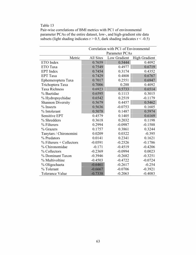
63

Table 13 Pair-wise correlations of BMI metrics with PC1 of environmental parameter PCAs of the entire dataset, low-, and high-gradient site data subsets (light shading indicates r > 0.5, dark shading indicates r < -0.5)

Correlation with PC1 of Environmental

Parameter PCAs Metric All Sites Low Gradient High Gradient

ETO Index 0.7659 0.5444 0.4092 ETO Taxa 0.7549 0.4977 0.6719 EPT Index 0.7454 0.3174 0.4352 EPT Taxa 0.7429 0.4808 0.6767 Ephemeroptera Taxa 0.7017 0.2551 0.6947 Trichoptera Taxa 0.7006 0.288 0.4092 Taxa Richness 0.6923 0.5733 0.6514 % Baetidae 0.6595 0.1113 0.3015 % Hydropsychidae 0.6542 0.2519 -0.1179 Shannon Diversity 0.5679 0.4457 0.5462 % Insects 0.5636 -0.0753 0.1605 % Intolerant 0.5078 0.1487 0.5974 Sensitive EPT 0.4579 0.1405 0.6169 % Shredders 0.3618 0.2032 0.1198 % Filterers 0.2994 -0.0987 -0.1588 % Grazers 0.1757 0.3861 0.3244 Tanytars / Chironomini 0.0209 0.0322 -0.395 % Predators 0.0141 0.2341 0.1621 % Filterers + Collectors -0.0591 -0.2526 -0.1786 % Chironomidae -0.171 -0.4519 -0.4206 % Collectors -0.2369 -0.0994 0.0023 % Dominant Taxon -0.3946 -0.2682 -0.3251 % Multivoltine -0.4503 -0.4722 -0.0724 % Oligochaeta -0.6461 -0.2617 -0.254 % Tolerant -0.6667 -0.0706 -0.3921 Tolerance Value -0.7338 -0.2063 -0.4083

64

sediment type, and physical habitat were all correlated with BMI metrics at low gradient

sites.

The environmental variables PCA of the high gradient site data subset differed from the

PCAs of the entire dataset and the low gradient site data subset. Rather than one

overwhelmingly important PC axis, the first two PCs of the high gradient site PCA

accounted for approximately equal portions of variance in the dataset. There were strong

positive loadings of some physical habitat parameters and DO and strong negative

loadings of SpC, alkalinity, hardness, and turbidity onto PC1. Strong positive loadings of

some physical habitat parameters as well as boulder and bedrock substrates onto PC2

were also evident, contrasted with strong negative loadings of sand and gravel substrates.

Despite this difference in the high gradient site PCA, BMI metrics similar to those in the

other two analyses were correlated with PC1 in this analysis. This indicates stronger

associations of BMI metrics with water quality and physical habitat than with substrate at

high gradient sites.

All three environmental variable PCAs detected a strong pattern wherein high physical

habitat scores and coarser substrates were contrasted with a correlated set of water quality

parameters (SpC, hardness, alkalinity, and turbidity) and finer substrates. In all cases,

high physical habitat scores and coarse substrates were correlated with BMI metrics,

indicating a less impacted BMI fauna. To the contrary, the set of water quality

parameters and finer substrates were correlated with BMI metrics indicating impacted

conditions.

3.10 Indices of BMI community integrity Community integrity rankings were developed separately for high and low gradient site

data subsets (Table 14). After eliminating metrics with low signal/noise ratios and

redundant metrics, similar sets of metrics remained; these were incorporated into

community integrity rankings (a biotic index, BI) for the gradient-specific subsets. For

the high gradient ranking system, more metrics were included that reflect specific

65

Table 14 BMI metrics included in the Biotic Indices created to discriminate more impacted sites from less impacted sites. Metrics marked with an asterisk (*) were considered indicators of impacted fauna, and scores on these metrics were weighted negatively in calculation of the Biotic Index.

Low Gradient High Gradient Taxonomic Richness Shannon Diversity EPT Taxa EPT Taxa ETO Index EPT Index Plecoptera Taxa % Hydropsychidae % Insects % Insects % Intolerant Tanytarsini / Chironomini % Multivoltine * % Multivoltine * Tolerance Value * Tolerance Value * % Dominant Taxon * % Collectors * % Grazers % Oligochaeta * % Chironomidae *

66

Table 15 Signal to noise (S/N) ratios of BMI metrics chosen for the low gradient and high gradient Biotic Indices, and Pearson product-moment correlations between these metrics and five environmental variables possibly indicating anthropogenic stress Low Gradient Metric S/N

Ratio Minimum DO

SpC Epifaunal Substrate

Fines Gravel

Tax Rich 9.45 -0.1388 -0.2561 0.3994 -0.3025 0.2724 EPT Taxa 9.31 0.1074 -0.2173 0.0627 -0.4432 0.2202 % Insects 5.33 -0.1565 0.2518 0.0287 0.0487 0.0260 ETO Index 5.63 -0.2149 -0.2037 0.3708 -0.1649 0.2563 T/C 4.78 0.2204 -0.3590 -0.0690 -0.2156 0.1124 %Intolerant 4.42 0.0637 -0.2184 -0.0143 -0.1645 -0.0247 Tol Value 3.85 -0.0865 0.2156 -0.1664 0.2589 -0.1651 %DomTaxon 3.83 0.1319 0.0427 -0.2730 0.0895 -0.2164 % Collectors 9.32 -0.0072 0.1975 -0.0688 -0.0704 0.0604 % Multivolt 7.14 -0.0017 0.3633 -0.3179 0.0502 -0.1376 High Gradient Metric S/N

Ratio Minimum DO

SpC Epifaunal Substrate

Fines Gravel

EPT Taxa 23.32 0.5239 -0.3970 0.3139 -0.2433 -0.0220 Plec Taxa 9.35 0.4151 -0.3899 0.3514 -0.1885 -0.0606 EPT Index 6.80 0.2024 -0.2748 0.2525 -0.2313 0.0603 Sens EPT 7.98 0.4352 -0.3116 0.2946 -0.0354 0.0057 Shan Div 3.25 0.3792 -0.4002 0.3089 -0.1917 -0.0165 Hydro 3.08 -0.2464 0.0366 0.0505 -0.3055 -0.0701 % Insects 8.18 0.2003 -0.1219 0.2863 -0.2773 -0.1062 % Grazers 7.19 0.4163 -0.2935 0.3244 -0.3529 -0.1087 % Multivolt 3.41 0.0157 0.0985 -0.0667 0.1414 0.0905 % Oligos 3.22 -0.1271 0.3035 -0.3316 0.1899 0.1798 % Chiros 5.97 -0.2117 0.4676 -0.2784 0.2177 -0.0866 Tol Value 9.48 -0.1739 0.3352 -0.4708 0.4416 0.0404

67

portions of intolerant EPT orders, including the number of Plecoptera taxa and percent

Hydropsychidae. The metrics chosen for low gradient ranking system included the ratio

of Tanytarsini to Chironomini midges (expected to increase with higher dissolved oxygen

concentrations). The concept is that this ratio is a useful indicator of relative BMI

community integrity in areas impacted by sedimentation, where midges thrive. Both

ranking systems included measures of BMI diversity, EPT diversity and taxa tolerance.

Correlations of candidate metrics with five environmental variables possibly indicative of

anthropogenic stress were used to choose which of two metrics to include in a BI, when

two metrics were highly correlated. These correlations are shown in Table 15.

BI scores were calculated separately for each transect, providing three scores per site for

each sampling event. The BI scores are summarized by site in Tables 16 and 17 and are

mapped by waterway in Figs. 20 to 28. In both low and high gradient site datasets, fall

BI scores were significantly higher than spring scores (low gradient: matched pairs t-test,

t20 = -4.06, P = 0.0006; high gradient: matched pairs t-test, t24 = -3.17, P = 0.0041).

While fall BI scores were higher than spring scores in both low and high gradient

datasets, a comparison of the ability of BI scores to distinguish site-to-site differences

based on F-score magnitude from between-site ANOVAs suggested that resolution of

between-site differences was higher in the spring at low gradient sites, resolution of

between-site differences was higher in the fall at high gradient sites (Low Gradient fall:

1-way ANOVA, F21,101 = 5.9417; Low Gradient spring: 1-way ANOVA, F22,109 =

9.8593; High Gradient fall: 1-way ANOVA, F26,102 = 16.4742; High Gradient spring:

1-way ANOVA, F24,119 = 7.6293). At some sites the BI was relatively high or low

independent of season, while other sites fluctuated widely in relative BMI community

integrity between seasons (Tables 16 and 17). BI scores at high gradient sites were lower

in urban areas. At ADW low gradient sites BI scores tended to be lower in upstream

compared to downstream sites.

Among low gradient waterways, BI scores were highest in Pleasant Grove Creek (Fig.

28). Pleasant Grove Creek is an urban low gradient waterway in western Placer County

exposed to minimal agricultural influence. Of the low gradient ADWs, BI score was

68

highest in Wadsworth Canal (Fig. 26). Among the high gradient sites, BI score was

highest in Auburn Ravine (Fig. 20), while Dry Creek and its tributaries scored lowest

(Fig. 22). Dry Creek has a higher percentage of urban land use than other high gradient

waterways, and is effluent-dominated during low-flow periods.

Pair-wise correlations between BI scores and physical habitat scores showed that both

low gradient and high gradient BI scores were correlated with the total habitat score

(Pearson product-moment correlations, low gradient: r2 = 0.0871, P = 0.0061; high

gradient: r2 = 0.1806, P < 0.0001; see figs. 29 and 30). Among low gradient sites, the

physical habitat components most strongly correlated with BI score were riparian zone

width, pool variability, and epifaunal substrate (Pearson product-moment correlations,

pool variability: r2 = 0.0939, P = 0.0043; epifaunal substrate: r2 = 0.0895, P = 0.0054;

riparian zone width: r2 = 0.0466, P = 0.0478). Among high gradient sites, the physical

habitat components most strongly correlated with BI score were epifaunal substrate, pool

variability, and sediment deposition (Pearson product-moment correlations, epifaunal

substrate: r2 = 0.1806, P < 0.0001; pool variability: r2 = 0.1377, P = 0.0003; sediment

deposition: r2 = 0.1158, P = 0.0009).

3.10.1 Seasonal site comparisons

To evaluate possible variation and reliability of metrics between seasons, a separate

biotic index was constructed for spring and fall in each gradient-specific dataset (Table

18). A notable difference between the general and season-specific BIs for low gradient

sites was the inclusion of a greater number of EPT taxa component measures in the

season-specific BIs. Percent grazers was a metric included in every high gradient site BI,

while the ratio of Tanytarsini/Chironomini was a metric included in all low gradient site

BIs. Percent multivoltine organisms and percent insects metrics were included in all BIs

except at high gradient sites in spring.

BI site scores were higher in fall than spring at most high and low gradient sites. In the

high gradient dataset, the taxonomic basis of this pattern is clear. That is, EPT taxa

occurred at higher taxonomic richness and abundances in fall. Taxa following this

69

Table 16 Mean biotic index scores of fall and spring samples at low gradient sites, including 95% confidence intervals

Fall Spring Site Mean BI 95% CI Mean BI 95% CI GS1 49 5.4 29 3.2 JS1 56 7.5 51 6.7 JS2 50 14.2 28 6.6 JS3 31 7.4 27 2.2 MD1 66 8.3 60 12.1 MD2 64 12.6 52 7.1 MD9 50 4.4 36 9.0 MD3 58 21.8 36 9.2 MD4 46 8.1 37 4.8 MD5 22 2.6 42 3.8 MD6 31 5.2 24 6.6 PG1 57 13.3 55 16.6 PG2 50 25.0 43 7.3 PG3 64 10.5 57 9.4 PG5 50 9.2 47 5.5 WC6 91 5.6 63 8.4 WC1 64 20.2 58 10.6 WC2 28 6.8 20 4.8 WC3 40 10.0 15 8.7 WC4 62 16.3 44 7.3 WC5 79 8.5 27 15.0

70

Table 17 Mean biotic index scores of fall and spring samples at high gradient sites, including 95% confidence intervals

Fall Spring Site Mean BI 95% CI Mean BI 95% CI AR2 49 8.2 29 11.4 AR3 70 7.3 63 16.6 AR4 85 11.0 59 15.1 AR5 65 2.6 34 8.9 AR6 66 3.2 34 10.0 AR7 31 8.8 26 12.7 BC1 50 5.4 32 11.2 BC2 64 5.8 68 9.2 BC3 68 7.6 74 10.0 DC02 40 8.7 26 14.2 DC03 35 4.1 33 16.4 DC04 32 5.1 44 4.3 DC05 34 5.5 27 3.1 DC06 52 3.7 40 8.4 DC08 43 1.4 46 8.0 DC09 36 2.5 44 6.3 DC10 35 4.0 30 11.9 DC11 38 11.5 45 1.8 DC12 44 4.1 33 11.1 DC13 40 6.0 23 5.8 WW1 43 4.1 56 3.6 WW2 40 5.2 31 8.5 WW3 45 1.0 43 7.2

71

0

10

20

30

40

50

60

70

80

90

100

AR2 AR3 AR4 AR5 AR6 AR7

Biot

ic In

tegr

ity S

core

FallSpring

Dow nstream Upstream

Fig. 20. Biotic index scores in Auburn Ravine waterway. Each bar represents the mean BI score and 95% confidence interval of the BI scores measured in a site during a given season (6 transects, 3 transects in each of 2 years).

72

0

10

20

30

40

50

60

70

80

90

100

BC1 BC2 BC3B

iotic

Inte

grity

Sco

re

FallSpring

Dow nstream Upstream

Fig 21. Biotic index scores in the Butte Creek waterway. Each bar represents the mean and 95% confidence interval of the BI scores measured in a site during a given season (6 transects, 3 transects in each of 2 years).

73

Fig. 22. Biotic index scores in Dry Creek waterway. Each bar represents the mean BI score and 95% confidence interval of the BI scores measured in a site during a given season (6 transects, 3 transects in each of 2 years).

0

10

20

30

40

50

60

70

80

90

100

DC02 DC12 DC13 DC03 DC06 DC04 DC05 DC10 DC08 DC09 DC11

Biot

ic In

tegr

ity S

core

FallSpring

Dow nstream UpstreamDry Creek Mainstem Antelope Creek Miner's RavineLindaCreek

74

0

10

20

30

40

50

60

70

80

90

100

WW2 WW3 WW1

Bio

tic In

tegr

ity S

core

FallSpring

Dow nstream Upstream

Fig. 23. Biotic index scores in Coon Creek waterway. Each bar represents the mean BI score and 95% confidence interval of the BI scores measured in a site during a given season (6 transects, 3 transects in each of 2 years).

75

Fig. 24. Biotic index scores in the Jack Slough waterway. Each bar represents the mean and 95% confidence interval of the BI scores measured in a site during a given season (6 transects, 3 transects in each of 2 years).

0

10

20

30

40

50

60

70

80

90

100

JS1 JS2 JS3

Biot

ic In

tegr

ity S

core

FallSpring

Dow nstream Upstream

76

Fig. 25. Biotic index scores in Main Drainage Canal waterways. Each bar represents the mean and 95% confidence interval of the BI scores measured in a site during a given season (6 transects, 3 transects in each of 2 years).

0

10

20

30

40

50

60

70

80

90

100

MD1 MD2 MD9 MD3 MD4 MD5 MD6

Biot

ic In

tegr

ity S

core

FallSpring

Main Channel Tributary 1 Tributary 2Dow nstream Upstream

77

Fig. 26. Biotic index scores in Wadsworth Canal waterway. Each bar represents the mean and 95% confidence interval of the BI scores measured in a site during a given season (6 transects, 3 transects in each of 2 years).

0

10

20

30

40

50

60

70

80

90

100

WC6 WC1 WC2 WC3 WC4 WC5

Biot

ic In

tegr

ity S

core

FallSpring

Tributary 1 Tributary 2

Dow nstream Upstream

78

Fig. 27. Biotic index scores in the Gilsizer Slough waterway. Each bar represents the mean and 95% confidence interval of the BI scores measured in a site during a given season (6 transects, 3 transects in each of 2 years).

0

10

20

30

40

50

60

70

80

90

100

GS1

Bio

tic In

tegr

ity S

core

FallSpring

79

0

10

20

30

40

50

60

70

80

90

100

PG1 PG2 PG3 PG5

Bio

tic In

tegr

ity S

core

FallSpring

Dow nstream Upstream

Fig. 28. Biotic index scores in the Pleasant Grove waterway. Each bar represents the mean and 95% confidence interval of the BI scores measured in a site during a given season (6 transects, 3 transects in each of 2 years).

80

Fig. 29. Correlation of physical habitat score with low gradient BI score (r2 = 0.0871). Points indicate fall cluster membership: ▲ = LG Ag 1, □ = LG Ag 2, ● = LG Ag/Urban.

81

Physical Habitat Score

100 120 140 160 180 200

Hig

h G

radi

ent B

I Sco

re

0

20

40

60

80

100

Fig. 30. Correlation of physical habitat score with high gradient BI score (r2 = 0.1806). High sediment deposition score indicates little sediment deposition. Points indicate fall cluster membership: ● = HG Native 1, ▲ = HG Native 2, □ = HG Urban.

82

Table 18 BMI metrics included in season- and gradient-specific biotic indices created to discriminate more impacted sites from less impacted sites. Metrics marked with an asterisk (*) were considered indicators of impacted fauna, and scores on these metrics were weighted negatively in calculation of the biotic indices.

Low Gradient High Gradient Fall Spring Fall Spring Taxonomic Richness Shannon Diversity EPT Taxa Shannon Diversity Ephemeroptera Taxa EPT Index EPT Index EPT Taxa Trichoptera Taxa Trichoptera Taxa EPT Index ETO Index ETO Taxa % Intolerant % Intolerant % Baetidae % Grazers % Grazers % Insects % Insects % Insects Tanytarsini/Chironomini Tanytarsini/Chironomini % Multivoltine * % Multivoltine * % Multivoltine * % Dominant Taxon * % Oligochaeta * % Chironomidae * Tolerance Value * Tolerance Value * % Tolerant * % Collectors * % Filterers * % Filterers *

83

pattern included Baetidae, Tricorythodes, Hydropsyche, Heptagenia, Wormaldia, and

Odonata. In general, the filter feeding niche was filled by Hydropsyche in fall, but by

Simulium in spring. Since Hydropsyche is a trichopteran and Simulium is a dipteran, this

shift reduces scores on metrics measuring the richness and abundance of EPT taxa. The

pattern of low BI scores in spring at high gradient sites appeared to be related to higher

abundances of Naidid oligochaetes and chironomid taxa. Both oligochaetes and

chironomids factored negatively into the BI scores at high gradient sites.

Other common seasonal shifts that occurred in both low and high gradient sites were

Tanytarsini in fall giving way to Orthocladiinae in spring (both chironomids), and

Tubificidae in fall shifting to Naididae in spring (both oligochaetes). Since these shifts

were between related taxa, they did not affect BI scores, except for the

Tanytarsini/Chironomini ratio.

The signal/noise ratios of fall and spring BIs were compared to evaluate which BI gives

more power to detect site to site differences in BMI community integrity. The low

gradient spring BI had more power to detect differences between sites, while the high

gradient fall BI had more power to detect differences between sites (One-way ANOVAs:

low gradient fall: F21,101 = 5.9417, low gradient spring: F22,109 = 9.8593, high gradient

fall: F26,102 = 16.4742, high gradient spring: F24,119 = 7.6293).

3.10.2 Summary by watershed/waterway

Auburn Ravine and Butte Creek, the two waterways with the least impacted land use

profiles and instream habitats, scored highest on measures of BMI community integrity

(BIs). Dry Creek is a more urbanized, more impacted high gradient waterway, and sites

on Dry Creek received lower BI scores. In the comparison of sites surrounding Coon

Creek SMD 1 WWTF, decreases in BI score were detected downstream of the WWTF.

Differences in BI scores between low gradient waterbodies were small, but sites on

Pleasant Grove Creek, the low gradient waterbody with the least amount of agricultural

land use and the greatest amount of native vegetation, manifested higher BI scores than

84

most ADW sites. Some of the sites on low gradient ADWs scored lowest on the low

gradient biotic index.

3.10.2.1 Auburn Ravine (Fig. 20)

Auburn Ravine is a natural waterway that originates in the Sierra Nevada foothills near

the City of Auburn (396 meters elev.). The stream flows west until discharging into the

East Side Canal, and finally the Sacramento River. The upstream reaches of Auburn

Ravine are dominated by wastewater treatment plant effluent and urban runoff from the

City of Auburn. The most downstream portion of Auburn Ravine, below the City of

Lincoln (50 meters elev.), is dominated by agricultural activities during irrigation season.

All BMI sampling sites were located upstream of major agricultural activities in the

valley floor.

As a whole the Auburn Ravine waterway scored high in measures of BMI community

integrity. Sites AR3 and AR4, both high gradient sites with favorable instream habitat

and distant from urban areas, manifested the highest BIs. BIs at AR2, the most

downstream Auburn Ravine site, were somewhat lower. AR2 is lower gradient than the

other Auburn Ravine sites and consisted mostly of fine substrates, some gravel, and some

woody debris. AR5 and AR6, immediately downstream of the city of Auburn and

bracketing the Auburn WWTF, were comprised of similar taxa and characterized by

equivalent BI scores. BMI integrity scores were not significantly different between the

two sites (fall: Wilcoxon rank sum test, N = 9, P = 0.1113; spring: t-test, t10 = 0.555, P =

0.5909). Few gastropods and many Chironomids and Wormaldia (Trichoptera) were

noted at AR6 (upstream of the WWTF), while at AR5, gastropods (Planorbidae) were

numerous and Chironomids and Simulium were uncommon. The lowest BIs in Auburn

Ravine were at AR7, in the center of the Auburn urban area. A large portion of water

flowing through AR7 originates in storm drains of roads and parking lots. AR7 was

relatively taxa rich, but not EPT rich. A large influx of water enters the stream at a

Pacific Gas and Electric hydroelectric power station between AR7 and AR6. This water

is likely to be unpolluted relative to the storm drain water from the city of Auburn, and

may be the cause of the sizable increase in BI scores downstream of AR7.

85

3.10.2.2 Butte Creek (Fig. 21)

Butte Creek originates in the Sierra Nevada range east of the City of Chico (60 meters

elev.). Butte Creek is a natural waterway that flows into Butte Slough, the heavily aligned

Sutter Bypass, and Sacramento Slough before reaching the Sacramento River. For the

majority of the irrigation season, April through September, lower Butte Creek and Butte

Slough are dominated by supply and return flows for agricultural irrigation.

Butte Creek is the only snowmelt driven agriculture-dominated waterway, as opposed to

irrigation supply and return water driven, sampled in this study. The upstream most BMI

sampling site, BC3, is located adjacent to the City of Chico. At sampling site BC2, Butte

Creek is considered agriculture-dominated due to volume of irrigation supply and return

flows, and is surrounded by intensive agricultural land use. However, large (> 5 meters

high) levees are located between the creek and surrounding agricultural land (rice and

orchards). The most downstream BMI sampling site on Butte Creek (BC1) is located at

the transition from Butte Creek into Butte Slough. This transition zone is characterized by

a slower flowing, deeper, and warmer waterway. Further, the substrate changes from

coarse boulder, cobble, and gravel to more fine material such as silt and clay in this

transition zone.

BI scores of upstream sites BC2 and BC3 were high, while BIs of BC1 were lower.

Habitat at BC2 and BC3 was very good, with large percentages of cobble substrates.

These sites are upstream of most agriculture, though some orchards are nearby. While

BIs at most other sites were high in fall, BC2 and BC3 scored somewhat higher in spring.

These two sites receive a high volume of cold water from snowmelt in spring. While

many other sites were characterized by fewer EPT taxa in spring, cold water

Ephemeroptera taxa such as ephemerellids and heptageniids increased at BC2 and BC3 in

spring. BC1 is surrounded by agricultural land. BC1 followed the usual seasonal pattern

of lower BIs in spring. The fall to spring taxonomic shift included a change from many

Ephemeroptera (particularly Tricorythodes) to many Chironomidae.

86

3.10.2.3 Dry Creek (Fig. 22)

Dry Creek is an urban-dominated watershed that originates from a number of small

creeks in the Sierra Nevada foothills east of Roseville (49 meters elev.). Dry Creek flows

into Natomas East Main Canal and eventually the Sacramento River at Discovery Park.

The Dry Creek Watershed covers approximately 74,000 acres, 8,700 acres of which are

located within the City of Roseville. The primary streams in the Dry Creek Watershed

include Dry Creek, Cirby Creek, Linda Creek, Strap Ravine, Miner’s Ravine, Secret

Ravine, Antelope Creek, and Clover Valley Creek. Portions of Dry Creek are effluent-

dominated certain times of the year (primarily during low flow summer conditions).

There are a number of wastewater treatment plants discharging within the Dry Creek

Watershed. BMI community integrity was assessed above and below the Placer County

Sewer District 3 (SMD3) wastewater treatment plant in Miner’s Ravine and the City of

Roseville wastewater treatment plant on the lower mainstem reach of Dry Creek. In

addition, BMI sampling sites were selected in most major tributary streams of Dry Creek.

The Dry Creek watershed is almost completely urbanized with many point and non-point

sources of possible contamination. BMI community integrity at all sites along Dry Creek

with the possible exception of DC6, the most upstream site, appeared impacted relative to

the most diverse BMI communities examined in this study. DC2 and DC12 were located

downstream of a WWTF. DC13 was immediately upstream of the WWTF, while DC3

was located upstream of the WWTF and downstream of a railroad yard in the city of

Roseville. Communities at sites DC12 and DC13 were similar, with dominant

populations of Chironomidae and Naididae. Filter-feeding Hydropsyche and

Nectopsyche were more common at DC12, as would be expected at a site enriched with

organic matter. Higher populations of filter-feeding trichopterans may explain the

somewhat higher fall BI score at DC12 relative to DC13. BI scores of the upstream sites

were not significantly different than those of downstream sites (fall DC3 – DC2: t-test,

t10 = 0.236, P = 0.8185; fall DC13 – DC12: t-test, t4 = 2.538, P = 0.0641; spring DC3 –

DC2: t-test, t10 = -0.339, P = 0.7417; spring DC13 – DC12: t-test, t10 = -0.352, P =

0.7319). The similar BI scores of these four sites suggest that the WWTF they surround

had no discernable effect on BMI community integrity. DC4 and DC5 are located in

87

Antelope Creek, a natural creek with some cobble substrate and some depositional

habitat. At DC4, BIs indicated relatively impacted biological conditions despite cobble

substrate. The higher BI score in spring was related to a seasonal shift from clams and

flatworms (fall) to Hydropsyche and Baetis (spring). Though water at DC5 was fairly

clear and many crayfish were present, BIs at this site indicated an impacted community.

DC6 was the least biologically impacted site on Dry Creek. Substrate consisted of cobble

that was well-consolidated. BMI fauna was diverse. DC10, on Linda Creek, was located

in central Roseville; BI scores were low and equivalent to sites on Dry Creek. Sites DC8,

DC9, and DC11 were located in Miner’s Ravine. At all these sites BI scores were higher

in spring than in fall, divergent from the common pattern. DC8 and DC9 bracketed a

WWTF, but BI scores were similar at both sites. DC8 had marginally higher BI scores in

the fall, but BIs did not differ in spring (fall: t-test, t4 = 2.867, P = 0.0456; spring: t-test,

t10 = -0.523, P = 0.6122). The seasonal pattern at sites DC8 and DC11 relate to higher

EPT abundances in the spring, particularly Hydropsyche. The higher spring BI at DC9

was related to greater taxonomic diversity.

3.10.2.4 Coon Creek SMD 1 WWTF (Fig. 23)

Coon Creek originates in the Sierra Nevada foothills north of the City of Auburn (396

meters elev.). Coon Creek is a natural, ephemeral, creek that flows west to the East Side

Canal, and finally the Sacramento River. Upstream reaches of Coon Creek are dominated

by wastewater treatment plant effluent and urban runoff. The BMI sampling sites in the

upper Coon Creek watershed were selected to assess BMI community integrity upstream

and immediately downstream of the Placer County Sewer Maintenance District 1

(SMD1) Wastewater Treatment Facility (WWTF). Site WW1 is located in the upper

Coon Creek watershed upstream of the Placer County SMD 1. WW2 is downstream of

the WWTF and WW3 is situated on a tributary that flows into the main waterway

between the WWTF and WW2. A reverse seasonal pattern was observed at WW2 due to

high populations of Hydropsyche and Wormaldia (Trichoptera) in spring. Overall, the

downstream site WW2 showed lower BMI community integrity than the upstream sites.

In fall, WW1 and WW2 did not have significantly different BI scores (t-test, t4 = 1.852, P

88

= 0.1376), but WW2 tended to score lower. In spring, BIs were much lower at WW2

than at WW1 (t-test, t10 = 7.999, P < 0.0001). BI scores at WW2 were lower than at

WW3 in both seasons (fall: t-test, t4 = -6.061, P = 0.0037; spring: t-test, t10 = 0.0006, P

= 0.0006).

3.10.2.5 Jack Slough (Fig. 24)

Jack Slough is a small agriculture-dominated watershed north of Marysville (19 meters

elev.) that is tributary to the Feather River. The slough is bounded between the Feather

River on the north and west, and the Yuba River on the south. The slough is a modified

natural waterway that has been extensively realigned and reconstructed along its lower

portion for flood control and transport of agricultural supply and return water. The upper

portion of Jack Slough, upstream of Trainer Hills, flows in its original channels and

contains irrigation supply water from the Yuba River. We did not sample this portion of

the slough.

During irrigation season (March – August) the lower portion of Jack Slough is composed

of supply water mixed with return water from surrounding rice fields, and likely would

not flow without agricultural inputs. During the winter months, Jack Slough contains

stormwater runoff from surrounding agricultural lands and contains drainage from local

waterfowl wetland areas. BMI sampling sites on Jack Slough were selected to reflect a

gradient of agricultural land use. Sites JS2 and JS3 are immediately adjacent to rice

fields. JS1, the most downstream sampling site, is located in a semi-natural, less

managed, riparian area that is less than 2.5 kilometers upstream of the confluence into the

Feather River. A BI score gradient was observed in Jack Slough, from relatively intact

downstream BMI communities to relatively impacted upstream communities. This

gradient was associated with declining abundance of coarse substrates, lower water

quantities in the channel, and increasing abundance of submerged macrophytes. While

submerged macrophytes created more potential BMI habitat, the abundance of

macrophytes probably created anoxic conditions that were partially responsible for lower

BIs. Jack Slough BMI fauna was dominated by Crangonyx amphipods, oligochaetes, and

chironomids.

89

3.10.2.6 Main Drainage Canal (Fig. 25)

The Main Drainage Canal (Main Drain) consists of a network of modified natural

(Hamlin Slough) drainage channels, historically natural drainage channels, and partially

constructed laterals that have been extensively aligned and modified for conveying

irrigation supply and return water for surrounding agricultural land practices. Irrigation

water is supplied to the Main Drain from the Sutter Butte Canal that contains Feather

River water from the Thermalito Afterbay. Flow in Main Drain goes into Cherokee Canal

and then enters Butte Sink, Butte Slough, and eventually Sacramento Slough and

Sacramento River. Peach and prune orchards are prominent in the upper watershed, while

rice dominates in the lower Main Drain watershed. The primary channel of the Main

Canal (Hamlin Slough) flows through the small town of Gridley (28 meters elevation) at

sampling site MD7.

Stream bank channels in the Main Canal are unstable due to a lack of riparian cover

related to agricultural practices including close proximity of crops, and heavy physical

stream channel maintenance conducted to maintain adequate irrigation and return water

flows. All sampling sites within the Main Drain have substrates dominated by mud.

Tolerant taxa are ubiquitous in the Main Drain, especially chironomids and oligochaetes.

Similar to other low gradient agriculture-dominated waterways, the Main Drain

manifested the trend of having higher BI scores at the more downstream sites. This

pattern was most likely related to the increase in substrate and physical habitat quality at

the downstream sites (MD 1 and MD 2) compared to the upstream sites (MD3 to MD8).

MD1 was the most downstream site on the Main Drain system and is subject to the

cumulative effects of seasonal irrigation and return water augmentation, stormwater

pulses, and local land management practices throughout the watershed. MD1 and MD2

are both depositional habitats, although MD 1 is subject to extremely variable flow

conditions. BI scores at MD1 and MD2 were the highest in the Main Drain. These sites

also consisted of the best habitat and substrates in this waterway, including some gravel

and abundant submerged macrophytes. BI scores at sites MD3 and MD4, both located on

90

one lateral of the Main Drain, were intermediate. Sites MD5 and MD6, both located on

another lateral of the Main Drain, were characterized by extremely impacted BMI

communities. Sites MD3, MD4, MD5, and MD6 were adjacent to agricultural land use.

While site MD3 consisted of some gravel and rip-rap substrates mixed with mud and site

MD5 appeared to be more eutrophic than other Main Drain sites, no major differences in

habitat or substrate were noted. This may indicate that differences in water quality were

responsible for much of the variation in BI scores among upstream sites in the Main

Drainage Canal.

MD9 was located at the nexus of the Main Drain and the Sutter Butte supply water canal,

and upstream of most agricultural return water inputs. BIs at MD9 were not particularly

high compared to other sites on the Main Drain. Regardless of intermediate BI scores,

taxonomic diversity at MD9 was greater than at all other agriculture-dominated, low

gradient sites. During this study, MD9 was not entirely removed from agricultural

practices effects. On 18 January 2001, a cropduster applying esfenvalerate (a pyrethroid

insecticide) to orchards oversprayed resulting in direct application on the Main Drain at

MD9. At or near this site, esfenvalerate concentrations exceeded 2070 ng/L in the

surface microlayer and subsurface esfenvalerate concentrations reached 23 ng/L (Kuivila,

pers. comm.). Large numbers of dead aquatic insects were observed drifting in the

insecticide plume at MD8, including many Ephemeroptera, Plecoptera, Trichoptera,

Odonata, and Diptera (located < 1 km downstream from MD9).

To examine temporal and spatial trends in the benthic community after the overspray,

BMI samples were collected at MD9 and at the downstream sites MD8, MD7, and MD2

on 6 February (19 days post event), 27 March (48 days post event), and 10 May (104

days post event). While no clear pattern of recovery was observed, clear differences were

observed among sites. These data show clear site-to-site changes in BMI community

integrity, with MD9 and MD2, the most upstream and downstream sites, characterized by

higher BI scores than MD7 and MD8 (Fig. 31). BI scores at MD2 were significantly

higher in February than at later dates, while BIs were significantly lower in May than at

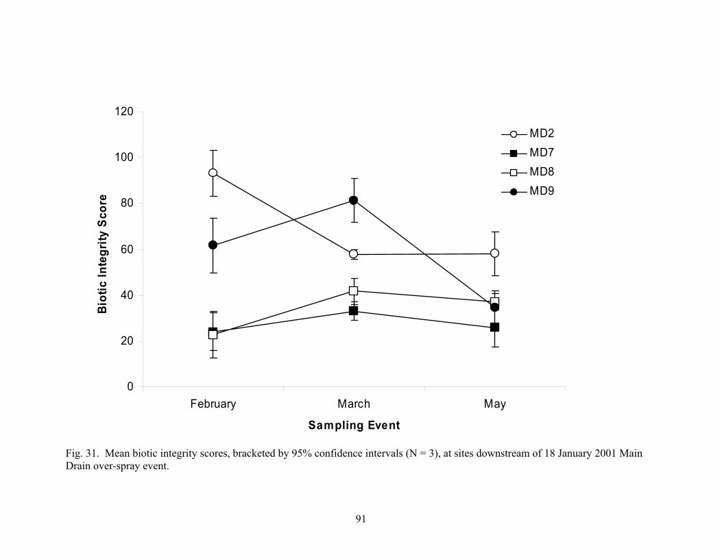
91

0

20

40

60

80

100

120

February March May

Sampling Event

Biot

ic In

tegr

ity S

core

MD2MD7MD8MD9

Fig. 31. Mean biotic integrity scores, bracketed by 95% confidence intervals (N = 3), at sites downstream of 18 January 2001 Main Drain over-spray event.

92

earlier dates. BI scores did not change significantly over time at either MD7 or MD8 (all

comparisons: 2-way ANOVA with Tukey’s multiple comparisons, P < 0.05).

Substrate and habitat were very poor at MD7 and MD8. This could account for the

extremely impacted BMI communities (consistently low BI scores). These sites did not

show “recovery” from the overspray. Substrate and habitat were relatively good at MD2,

and this site manifested overall higher BI scores and more temporal fluctuation. There

was no apparent recovery from the overspray event.

3.10.2.7 Wadsworth Canal (Fig. 26)

Wadsworth Canal is an agriculture dominated waterway that originates from water

diverted from the Feather River, a natural creek, irrigation return water from extensive

agricultural land east of the Sutter Buttes, and rainfall events. Wadsworth Canal consists

of a number of small laterals that, historically, may have served as natural flow routes for

rainfall runoff. Wadsworth Canal flows into the Sutter Bypass and Sacramento Slough

before reaching the Sacramento River. Live Oak Slough is a natural tributary of

Wadsworth Canal, which is a historical flood channel of the Feather River. There are

currently no natural flows in Live Oak Slough. Live Oak Slough carries urban runoff and

agricultural return water.

Habitat scores and substrates at Wadsworth Canal sites were comparable to those in the

Main Drain, yet BMIs at some Wadsworth Canal sites were more diverse and less

tolerant than at Main Drain sites. The spatial pattern of BI scores in Wadsworth Canal

was as in the Main Drain and Jack Slough, with downstream sites manifesting higher

scores. BI scores were highest at the two most downstream sites, WC6 and WC1. Sites

WC2 and WC3, a tributary to Wadsworth Canal, were both extremely biologically

impacted. These sites contained little water and their substrates were entirely composed

of mud. In contrast, sites WC4 and WC5, on another Wadsworth Canal tributary,

appeared only marginally more impacted than downstream sites. WC4 contained some

cobble and gravel substrates and some emergent vegetation. WC5 was characterized by

entirely sand substrates and masses of instream vegetation. WC5 was subject to some of

93

the lowest DO levels measured, possibly due to the large quantities of floating vegetation.

It is striking that despite very anoxic conditions, WC5 harbored a more intact BMI

community than sites WC2 and WC3.

3.10.2.8 Gilsizer Slough (Fig. 27)

Gilsizer Slough originates in Yuba City (18 meters elev.) and flows west in its original

channel into the Sutter Bypass. Gilsizer Slough is a natural waterway that has an

intensely managed riparian zone and channel. The slough is dominated by agricultural

return flows during the irrigation season (March – October). Urban runoff from Yuba

City at its headwaters and stormwater runoff during rain events are other sources of flow

to Gilsizer Slough. The sampling site (GS1) on Gilsizer Slough was located in the lower

agricultural dominated reach, and is adjacent to orchards. Flow is typically none to low

in the slough, and aquatic habitat most resembles lentic waterbodies except during the

winter rainy season.

Habitat scores at the Gilsizer Slough (GS1) site were the lowest of any in this study.

Flow was very low. Chironomids and oligochaetes dominated.

3.10.2.9 Pleasant Grove (Fig. 28)

Pleasant Grove Creek originates near Loomis (121 meters elev.) and flows west before

discharging into the Cross Canal, and finally the Sacramento River. Pleasant Grove

Creek is a natural, ephemeral, creek that is dominated by urban runoff from the

surrounding expanding development in Placer County. Agricultural return and supply

water dominates Pleasant Grove Creek during the irrigation season (March – October) in

the lower 4.5 miles from Pettigrew Rd. to the west. Only sampling site PG1 (Pleasant

Grove Creek at Pettigrew Rd.) and PG2 (Pleasant Grove Creek at Fiddyment Rd.), the

most downstream sites, are influenced by agricultural activities.

The Pleasant Grove waterway is low gradient, but surrounded by more native vegetation

than the other low gradient waterways, and is subject to urban inputs including

technology industry dischargers. The upstream-downstream gradient of increasing BI

94

scores seen in the more agriculture-dominated waterways was not observed on Pleasant

Grove Creek. Among the Pleasant Grove sites, BI scores were highest at PG1 and PG3.

PG1 is surrounded by native vegetation and characterized by the highest habitat scores of

all low gradient sites. PG3 is located at a large pond with clear water and abundant

macrophytes and algae. BI scores at PG2 and PG5 were slightly lower than at PG1 and

PG3. Site PG2 is a relatively deep pond with low flow. Chironomids and worms (both

tolerant of low DO) were dominant in both seasons at these sites. Site PG5 was near an

urban area, receiving much urban runoff. This site was eutrophic and turbidity was high;

chironomids, snails, and oligochaetes dominated. Despite the lack of intensive

agriculture in the Pleasant Grove drainage, the BI scores at Pleasant Grove sites were

lower than those at the least impacted agricultural drain sites (WC6 and MD1).

4. Discussion This study was designed to describe BMI communities and aquatic habitats in

agriculture- and urban (effluent)-dominated waterways in the lower Sacramento River

watershed. Within these waterways sampling sites were selected to reflect a gradient of

land use. Effluent dominated waterways included sampling sites above and below

WWTFs. Analyses revealed that while the overriding difference in BMI communities

occurred between high and low gradient waterways, much variation in BMI communities

is present among sites of each gradient type. A major contribution of this study was to

provide baseline information on BMI community structure and habitat information in

high gradient and low gradient waterways of the Central Valley. In both high and low

gradient waterways, cumulative effects of practices associated with agricultural and

urban land uses were linked to differences in the BMI community. Agriculture and

urbanization both affect waterway physical habitat and water quality that, in turn, impact

biological communities. Following is a discussion and interpretation of our results and

results of other relevant investigations including land use, physical habitat, water quality,

identification of stressors, bioassessment data variability, seasonal variation, and level of

taxonomic identification.

95

4.1 Waterway gradient A large number of insect taxa, including many sensitive species of the EPT taxa, depend

on fast-flowing, cold water for survival and health. Such sensitive taxa occur in high

gradient streams, but conditions in low gradient, low elevation streams typically exclude

the more sensitive EPT taxa. Our analyses identified indicator species representative of

both high and low gradient waterways. Such information will be useful for future

investigations in the lower Sacramento River watershed. Low gradient communities

consisted primarily of chironomid midges, damselflies, beetles, and non-insects such as

crustaceans, clams, and oligochaetes. High gradient communities included many

mayflies and caddisflies, stoneflies of the genus Bisancora, Corbiculacea clams, Argia

damselflies, and the pollution-sensitive beetle Optioservus.

When evaluating BMI communities or extent of perturbation, BMI data from sites with

different gradients should not be compared. When constructing Indices of Biological

Integrity (IBIs), care should be taken to select reference sites with equivalent gradient.

Either separate IBIs should be created for low and high gradient streams in a region, or a

multivariate model (e.g. RIVPACS, Clarke et al., 2003) should be constructed that

accounts for gradient-specific differences in BMI communities. This conclusion is an

extension of recommendations that ecoregion and watershed be considered in designing

bioassessment studies and in interpreting data (Bournand et al., 1996; Bowman and

Bailey, 1997; Omernik and Bailey, 1997; Brown and May, 2000).

BMI taxa at sites within individual waterways/watersheds tended to be similar. We are

not suggesting that BMI data be independently interpreted for each waterway. Rather, an

awareness of possible waterway-wide effects of stressors on BMIs may suggest that

solutions to BMI community integrity issues require consideration of all activities in the

watershed.

96

4.2 Land use

Wherever land is utilized intensively for agricultural or urban development, such

activities affect the ecology of both terrestrial and aquatic systems. In wadeable streams

such as those sampled in this study and in many other bioassessments conducted using

similar methods, BMI metrics indicate impacted communities in areas of agricultural and

urban development, where habitat, substrate, and water quality are degraded. Low-

gradient streams subject to more intensive agriculture were characterized by lower

diversity of insects, and higher numbers of chironomids and oligochaetes. High-gradient

stream reaches subject to more intensive urban development consisted of fewer EPT taxa

(especially pollution-sensitive EPT taxa) and greater numbers of chironomids. BI scores

indicated that sites subject to intensive agriculture or urban development manifested

lower BMI community integrity.

Other investigators have examined the association of agricultural and urban land use with

BMI community structure and metrics. Brown and May (2000) discovered that

agricultural and urban land uses were strongly associated (negative correlation) with

macroinvertebrate community structure and metrics in the lower San Joaquin River

watershed. Three streams in the Piedmont ecoregion of North Carolina were studied to

evaluate the effect of land use on water quality and aquatic biota (Lenat and Crawford,

1994).

Lenat and Crawford (1994) examined three streams: one forest-dominated, one urban-

dominated, and one dominated by agriculture. Only one site on each stream was

sampled, but sites were sampled in January, April, June, and November. The three

streams differed in regards to BMI community structure. The stream surrounded

primarily by forests was characterized by high BMI richness, especially intolerant EPT

groups (dominant taxa—mayflies), many unique species, and many intolerant species.

Similar to our findings, the agriculture-dominated stream was characterized, as in the

current study, by low EPT taxa richness, many tolerant taxa, and dominant populations of

chironomid midges. Because land use in this watershed was 48% row crops and 31%

forested, it is questionable that this stream effectively represented an agriculture-

97

dominated watershed. The urban stream site was the most highly stressed, characterized

by low taxa richness, many tolerant species, low abundance values, and few unique

species. Most species of mayflies, stoneflies, and caddisflies, numerous in forested areas,

disappeared in agricultural and urban waterways. They were replaced by Chironomidae

in agricultural areas and oligochaetes in urban areas. These authors attributed differences

in BMI community structure in the three streams to water quality factors. However,

neither instream habitat conditions nor riparian habitat were assessed in this study.

Absence of such data confounds inferences regarding effects of water quality on BMI

community structure.

Dance and Hynes (1980) studied invertebrate community composition in two stream

reaches in Ontario, Canada where agricultural land use adjacent to the reaches varied

considerably. These investigators concluded that intensive agricultural land use had

profound effects on BMI community integrity. BMI community integrity was more

impacted in the stream reach with more intense agriculture than in the reach with less

intense agricultural activities. Further, BMI communities were less diverse in both

agriculture-influenced streams than in unmodified streams of similar size and substrate.

A battery of in situ toxicity tests were used by Crane et al. (1995) to assess the effects of

agricultural land runoff on water quality in a stream in the United Kingdom. The primary

goal was to determine whether the in situ tests provided information consistent with BMI

bioassessment data. Results of in situ toxicity tests with an amphipod and a midge (larval

dipteran) were consistent with bioassessment data. Both confirmed impacts of

agricultural runoff.

Roy et al. (2003a) investigated the effects of urban land use on BMI community integrity

in the state of Georgia, and found that sites surrounded by more than 20 percent urban

land use scored no higher than a “fair” rating on an IBI.

While the application of bioassessments to assess the effects of agricultural land use on

aquatic ecosystem biological communities has been somewhat limited, other BMI

98

investigations document that farming activities degrade stream/river water quality and

habitat, significantly impacting BMI communities (Kendrick, 1976; Corkum, 1990;

Quinn and Hickey, 1990; Schofield et al., 1990; Delong and Brusven, 1998; Kay et al.,

2001).

Both agricultural and urban land use can cause sedimentation, pollution by runoff, and

loss of riparian vegetation, all of which can lead to impaired BMI community integrity.

As other authors have concluded (e.g. Roy et al., 2003a), this relationship between land

cover and reach-scale variables makes it difficult to separate the effects of various

stressors. The effects of land use correlated variables will be discussed in terms of

stressors to low and high gradient communities in following sections.

4.3 BMI community integrity We were able to develop BMI community integrity relative ranking systems (Biotic

Indices – BIs) were developed for low and high gradient streams. Both ranking systems

showed that sites more drastically affected by anthropogenic stressors such as

sedimentation, runoff pollution, and loss of riparian vegetation were characterized by

more biologically compromised conditions than sites exposed to less intense

anthropogenic stress. Accurate estimates of BMI community integrity at sites depends on

the existence of reference metrics determined from reference (or ‘least

disturbed/impacted’) sites sampled multiple times through time to account for spatial and

temporal variation (Barbour et al., 1996-1999; Gibson et al., 1996; Bailey et al., 2004).

In this report statements regarding BMI community integrity or BI scores at sites are not

‘absolute’, but rather relative to data collected in this project.

4.3.1 Low gradient waterways

In the current study, low gradient sites ranged from those with fauna dominated by

damselflies, chironomid midges, and snails (Pleasant Grove) to sites dominated by

oligochaetes and crustaceans (Main Drain and Wadsworth Canal). While sites on

agricultural drains were generally more impacted than sites on the less agricultural

Pleasant Grove waterway, some sites along agricultural drains, such as WC6 and MD1,

99

were characterized by higher BI scores than any site on Pleasant Grove. Downstream

sites in agriculture-dominated waterways tended to have higher BI scores than upstream

sites.

A study on the lower San Joaquin River watershed (Brown and May, 2000) yielded

results similar to our observations on low gradient sites. This analysis revealed two types

of low gradient sites in agriculture-influenced waterways, one dominated by baetid

mayflies and gastropods, the other dominated by amphipods and oligochaetes.

The Central Valley is a vast region of mostly low gradient waterways dominated by

intensively farmed land. Agricultural land use on such a scale is associated with chronic

and extreme sedimentation, reduced or absent riparian vegetation, and water quality

contamination by sediment, metals, nutrients, organic and inorganic pollutants, organic

wastes that affect oxygen availability and agricultural chemicals, including pesticides.

Compared to historical standards, the lack of or poor riparian zone vegetation,

particularly trees, has dramatically reduced the amounts of allochthonous coarse

particulate organic matter (CPOM- such as dead leaves and woody debris) entering

aquatic ecosystems.

Many studies documented that presence of allochthonous CPOM to be very important to

maintaining healthy BMI communities. CPOM is important both as a food source for

many BMI taxa, and as a source of habitat. Richardson (1991) confirmed the importance

of CPOM for maintaining high densities of invertebrates, and suggested that seasonal

food limitations may lead to seasonal changes in BMI biota. By excluding terrestrial

litter inputs and removing small woody debris, Wallace et al. (1999) reduced the biomass,

abundance, and total secondary production of BMIs in areas of mixed substrate. The

BMI communities of reaches dominated by bedrock substrates were not affected by the

removal and exclusion of CPOM.

In low gradient agricultural areas of the Central Valley, CPOM has been replaced as an

energy source by fine particulate organic matter (FPOM) originating from fertilizers and

animal waste products. The increase in sedimentation and change in energy source

100

resulted in BMI communities dominated by FPOM utilizing mud-dwelling organisms.

Riparian vegetation, instream habitat, water quality, and the dominant pathways of

energy flow through these ecosystems are therefore intimately intertwined, and the

combination of these factors determines the integrity of the aquatic ecosystem, including

the BMI community.

4.3.2 High gradient waterways

High gradient sites generally scored higher on measures of community integrity than did

low gradient sites. However, a wide range of BMI integrity was noted at high gradient

sites. The major gradient in community integrity appeared to be associated with land use.

Sites in more intensively developed urban areas showed lower community integrity than

those surrounded by more native vegetation. Sites with more intact BMI communities

consisted of higher proportions of sensitive EPT taxa, while more impacted sites

contained fewer EPT and more chironomids.

This study reflects trends similar to those observed by other examinations of BMI

communities in urban areas, confirming that urban development can have deleterious

effects on BMI communities. One case is that of the Buffalo River in the metropolitan

area of Buffalo, New York, where pollution caused virtual extinction of the entire BMI

community by the 1960’s. Forty years of remediation have improved the community to

the point where oligochaetes and chironomids (pollution-tolerant taxa) are now plentiful,

and many other insect taxa are beginning to re-establish populations (Diggins and

Snyder, 2003).

Rogers at al. (2002) measured both metals contamination and habitat degradation in

urban areas. They found that physical and chemical stressors arising from urban

development act additively to increase impairment of BMI communities. Moreover, they

found that physical impairment often masks effects of metals contamination.

101

4.4 Physical habitat Physical habitat, including riparian vegetation, is a major determinant of aquatic

biological community potential (e.g., Karr, 1991; Richards et al., 1997; Barbour et al.,

1999). While chemical pollution continues to be an issue in many freshwater

ecosystems, habitat degradation is considered responsible for more biological impairment

than that caused by chemicals (Rankin, 1995). According to Cooper (1993), protection

and remediation of habitat are the most effective means of conserving and restoring

aquatic ecosystem biological diversity. Irrespective of this knowledge, little regulatory

attention has focused on protection of aquatic and riparian habitat (Hughes et al., 1990;

Karr, 1991-1993; Rankin, 1995), the focus being primarily on contaminants.

4.4.1 Low gradient waterways

Even among highly degraded low gradient waterways of the Central Valley, a range of

habitat quality is evident. Coarse substrates and higher physical habitat scores were

associated with higher BI scores at low gradient sites. Sites with plentiful submerged or

emergent macrophytes (e.g. MD1) or relatively ample gravel substrates (e.g. WC4)

contained more diverse BMI fauna than mud-dominated sites with few plants (e.g. WC2).

Correlations of BI scores with physical habitat measures indicated that, along with pool

variability and epifaunal substrate, riparian zone width significantly associated with BMI

community integrity. Riparian zone width affects the amount of allochthonous plant

matter that washes into a stream. Perhaps more importantly, the riparian zone can

improve water quality by filtering many of the contaminants present in runoff from the

land surrounding a waterway, including excess nutrients, sediment, metals, and pesticides

(Muscutt et al., 1993; Lin et al., 2002). This finding suggests that increased protection of

riparian areas, including the widening of undeveloped riparian zones, would help to

improve the integrity of aquatic ecosystems in the Central Valley.

Downstream ADW sites, with greater flow and larger channels, manifested higher BI

scores. For example, a notable increase of BI scores was observed in three Jack Slough

sites from upstream to downstream. This trend also was observed in the Main Drain

Canal and Wadsworth Canal. Further investigation is necessary to elucidate whether

102

factors other than stream flow and size are responsible for the higher downstream BI

scores.

The importance of coarse substrates, instream habitat, and instream vegetation suggests

that sedimentation, prevalent in ADWs, is a major obstacle to BMI community integrity.

Relatively robust BMI communities can exist without coarse substrates in the presence of

appropriate vegetation (e.g. MD1); a fruitful avenue to restoring BMI community

integrity in low gradient waterways may include ensuring the presence of healthy plant

communities. Prior to implementing such a restoration strategy, investigations into

factors that preclude adequate vegetation in these waterways as well as into inhospitable

DO levels resulting from overgrowth of instream vegetation (e.g., nutrients, low flow,

high temperatures, etc.) would be needed.

There can be little doubt that hydrology factors (no flow, little flow, fluctuating flows)

and physical alteration (plus maintenance activities) of waterways in the Central Valley

have considerable impacts on biological communities. This study was not designed to

assess the effects of these factors on BMI community integrity.

4.4.2 High gradient waterways

In urban watersheds chemical contamination commonly accompanies physical alteration

of stream and riparian habitat. Correlations of high gradient BI scores with physical

habitat signified that good instream conditions (including woody debris, root mats, leaf

litter, and coarse substrates) and lack of sedimentation were the most important

components to healthy BMI communities. This implies that sediment in urban runoff has

the potential to significantly decrease BMI community integrity. Controlling erosion and

inputs of sediment from construction and other urban activities would protect BMI

community integrity. Apart from controlling sedimentation, we recommend preservation

of existing instream and riparian habitat and restoration of instream and riparian habitat at

sites with impacted BMI communities. Other investigations (e.g., Jones and Clark, 1987;

Diamond et al., 2002; Rogers et al., 2002) documented that urbanization has severe

impacts on aquatic biological communities.

103

4.4.3 Relevant studies

Similar to our results, other investigators have identified physical habitat factors as

significant determinants of BMI community structure and metrics in California’s Central

Valley. Brown and May (2000) investigated associations between macroinvertebrate

assemblages on large woody debris and environmental variables in the lower San Joaquin

and Sacramento River drainages. Analogous to our results, their analyses indicated that

dominant substrate type, stream gradient, specific conductance, water temperature,

percentage of basin in agricultural land use, and percentage of basin in combined

agricultural and urban land use were the likely determinants of macroinvertebrate

assemblages. The importance of substrate to BMI communities was documented by

observations that the communities of two natural channels came to resemble the

communities of agricultural drains after a flooding event resulted in massive deposition

of sediment. The change in community composition involved a loss of many EPT taxa

and an increase in abundance of chironomids and oligochaetes.

Griffith et al. (2003) examined relationships between environmental gradients and

macroinvertebrate assemblages in the Central Valley portions of the Sacramento and San

Joaquin River watersheds. According to these authors the probable primary

environmental determinants of BMI assemblages in the Central Valley are instream

habitat, including substrate type: (1) By metrics analysis—channel morphology and

substrate, and (2) By taxa abundance analyses—specific conductivity, channel

morphology, and substrate. Channel management activities and landscape scale

alterations of catchments by agriculture were identified by these authors as the major

activities responsible for the environmental factors determining BMI assemblages. In

this study, comparable to our results, more homogenous instream habitat and substrate

was associated with lower taxa richness and higher mean tolerance value. Although site

cluster analyses were performed, there was no information provided regarding location of

the sites in the clusters. No inferences were made regarding BMI community integrity at

sites in the study. One of their goals was to identify metrics and indicator taxa indicative

of specific stressors. This goal was not achieved. Griffith et al. recommended a

104

multivariate approach that assesses sites with the BMI assemblage as an indicator unit

instead of specific indicator taxa. According to these authors BMI metrics determined in

their study could be incorporated into an ecoregion-specific index of biotic integrity that

could be applied to diagnose associated environmental variables. However, this

application was not incorporated into their article. Neither was there a ranking of sites

relative to an index of biotic integrity. Neither seasonal nor year-to-year variations in

BMI assemblages or metrics were assessed in this study.

The primary goal of a study conducted by Hall and Killen (2001) was to characterize

physical habitat and BMI communities in Orestimba Creek (an agriculture-dominated

stream that discharges into the San Joaquin River) and Arcade Creek (an urban creek in

Sacramento that discharges into Steelhead Creek) a tributary to the Sacramento River. A

second objective of this study was to assess potential impacts of organophosphorus (OP)

insecticides, particularly chlorpyrifos, on BMI communities in these two streams. The

CSBP procedure was applied to ten sites on each creek. The Hall and Killen report

provides a qualitative characterization of some physical habitat factors in Orestimba and

Arcade Creeks in late spring. BMI communities in both creeks were relatively

impoverished and dominated by oligochaetes and chironomids. Bank stability, bank

vegetation, and sinuosity were reported to be the physical habitat variables most likely

influencing BMI community metrics.

Results of the current study are consistent with findings of Griffith et al. (2003) as well as

Hall and Killen (2001). Stream size, the extent of channel alteration, extent of channel

sinuosity, vegetation, and bank stability, along with other aspects of physical habitat, are

important determinants of BMI community integrity.

Roy et al. (2003b) examined the effects of sedimentation on BMI communities, reporting

that sedimentation reduced taxa richness. The effects of sedimentation were more drastic

in riffle habitats than in bank habitats. Roy et al. suggested that bank and snag habitats

act as refugia for BMIs during periods of sedimentation, and that taxa that facultatively

inhabit bank habitats are more likely to survive sedimentation than taxa obligately

105

inhabiting riffles. Maintaining or restoring taxa richness and optimum health to high

gradient waterway BMI communities will require minimizing sources of sedimentation

(such as erosion from urban development, agriculture, and silviculture) to maintain

populations of insect taxa obligately inhabiting riffles. The findings of Roy et al. (2003b)

strengthen the argument that CPOM is important to BMI communities as a source of

habitat. After a waterway has experienced a large sedimentation event that covers coarse

substrates, allochthonous CPOM is likely to be the only source of new habitat for taxa

that inhabit coarse substrates. CPOM is, therefore, crucial to maintaining taxa richness

during periods of sedimentation.

4.5 Water Quality According to Barbour et al. (1996), ‘a clear distinction between impacts due to a

combination of large-scale habitat alteration and water-quality degradation is often not

possible.’ Design of the current study was not such that water quality and physical

habitat effects on BMI community integrity could be definitively distinguished. Further,

few bioassessment studies, including the current one, have thorough/complete water

quality data. The range of variables included is usually incomplete and detection limits

for many variables inadequate. Frequency of measurement is typically sub-optimal.

While physical habitat factors remain relatively constant temporally, many water quality

variables vary considerably through time. Habitat features and water quality parameters

often covary, confounding attempts to discriminate the factors most responsible for BMI

community perturbations. Each water quality variable is measured independently, but

BMI communities almost certainly respond to additive, synergistic, and/or cumulative

effects. Statistical analyses cannot detect all water quality variable interactions. For

example, water quality variables a, b, c, and d may be at concentrations that do not

correlate with (and individually, are below published effect levels) with BMI metrics, but

a+b+c+d evoke an additive, synergistic, or cumulative effect on BMI community

integrity. This study confirmed depauperate physical habitat conditions in many Central

Valley waterways, especially low gradient waterways. These conditions constrain the

ability of bioassessments to discern water quality impacts on BMI communities. Given

these limitations, we do not recommend standard BMI bioassessment as a stand-alone in

106

attempts to evaluate water quality (including the presence of contaminants), especially at

sites with poor to moderate physical habitat conditions.

4.5.1 Low gradient waterways

Some associations between water quality variables and BMI metrics were discovered in

this investigation. Correlations implicated SpC, hardness, alkalinity, and phosphorus as

specific water quality components likely influence BMI community integrity. DO and

pH also varied between sites in the low gradient dataset, but neither of these parameters

was associated with differences in BMI community integrity. Downstream sites tended

to have higher BI scores than upstream sites. Water quantity improvements between

upstream and downstream sites may be responsible for this downstream increase in the

integrity of BMI communities, possibly because larger volumes of water downstream

dilute contaminants that were more concentrated in some upstream reaches. It should be

emphasized that this study did not include streams containing source water, upstream

from any agricultural influence. The majority of the upstream sites in the low gradient

dataset were small tributaries containing return water, likely to be most intensively

exposed to stressors from agricultural activities. Some indications of tributary-specific

water quality effects on BMI communities were noted. For example, at Main Drain sites

MD5 and MD6, situated on the same tributary, habitat quality was equivalent to that

occurring at site MD4, yet BI scores at these two sites were lower than at MD4.

Potentially degraded water quality in the MD5 /MD6 tributary may have been responsible

for the lower BI scores.

To more effectively use bioassessments to evaluate low gradient waterway biotic

conditions, procedures and study designs should be refined so that water quality and

physical habitat variable effects on BMI community integrity can be more effectively

distinguished. Probabilistic-based sampling designs are inappropriate when a primary

objective is to assess potential water quality effects on macroinvertebrate communities

because such an approach is unlikely to include gradients of water quality parameters of

interest. Approaches that may be useful for discriminating water quality effects include

use of artificial substrates, trend monitoring (frequent, consistent, and long-term

107

monitoring of water quality parameters) and event-based sampling to track changes in

BMI community integrity at specific sites, point source studies bracketing areas

suspected to be the origin of water quality concerns, and studies designed to minimize

habitat variation while investigating water quality parameter gradients.

The basic concept of artificial substrate studies is to standardize substrate so that water

quality parameters are the primary variables. While artificial substrate procedures have

several limitations, they can be very useful components for assessing potential water

quality issues if objectives remain simple and if inferences from data gathered do not

exceed procedure capabilities. Taxonomic diversity and proportional abundance are

measures that are usually within the capacity of artificial substrate procedures.

In the absence of reference sites, frequent, consistent, and long-term monitoring of water

quality parameters of interest (trend monitoring), coupled with event-based

macroinvertebrate sampling (e.g., rain event or ‘first flush’ sampling), could be

informative because each site would serve as its own control when examining temporal

variations in BMI community integrity. Such sampling requires identification of sites

appropriate to the larger population of sites that the bioassessment results are intended to

represent, and also necessitate recognition of events that potentially affect BMI

communities or a large investment in routine sampling of a large number of sites.

Continued trend monitoring can be especially useful in detecting effects of water quality

parameters because, at a given site, physical habitat features are less likely to change over

time whereas temporal variation of water quality can be considerable. Thus, frequent

sampling of macroinvertebrates and water quality parameters allows for correlation

analysis between BMI metrics and water quality parameters.

Point source study designs bracket suspected sources of water quality problems to

investigate possible impacts resulting from those sources. With such designs care must

be taken to select sites with similar habitat, including substrate, flow, vegetation in the

channel, and riparian zone characteristics. It is also possible to design studies that assess

BMI community integrity between populations of sites differing in water quality

108

parameters, but in such cases it is essential to control or account for, not only differences

in BMI communities resulting from habitat differences, but also differences related to

watershed-level factors and processes.

Lack of historical data prior to intensive agricultural land use and extensive use of

pesticides, as well as other agricultural chemicals, precludes an understanding of BMI

communities that did and should exist in ADWs. A study by Heckman (1981) cataloged

the taxa of an orchard’s irrigation system. This cataloging was performed because, just

prior to the use of DDT, another scientist thoroughly cataloged taxa in the same irrigation

system. The only major difference between the two cataloging events is decades of

modern pesticide use. Results show that many taxa were extirpated from the system;

however, several taxa apparently adapted and thrived in the presence of pesticides.

Various resistance mechanisms and natural immunity weigh heavily in explaining the

presence of the remaining taxa. The predominant taxa consisted of midges, oligochaetes,

and flatworms. In support of Heckman’s findings, a similar taxa list was garnered by

Lugthart and Wallace (1992) after repeatedly treating a stream with methoxychlor to

purposefully remove BMIs. Further investigations may reveal that BMI communities in

ADWs are unaffected by low-magnitude agricultural chemical water quality degradation

and/or that communities (dominated by resistant taxa with short life cycles) recover

quickly to high concentration spikes of these chemicals. On the other hand, BMI

communities in particular ADWs may have been degraded to a baseline condition such

that little or no response to further water quality degradation can be detected. If this is

the case, BMI bioassessments will be of little value to regulatory agencies in these types

of waterways, with the possible exception of restoration projects. Rogers et al. (2002)

suggested that effects of contaminants on macroinvertebrate communities can be masked

if stream channelization, loss of riparian vegetation, or other physical stressors exert

comparable or larger influences.

During the course of this study an insecticide overspray of the Main Drain was observed.

Our field observations suggest that such events are relatively common. Immediately after

the event large numbers of dead macroinvertebrates were collected. Preliminary

109

evidence concerning changes in BMI community integrity following the event indicates

no notable ‘recovery’ in BMI communities downstream of the overspray over the

following months. Worms and chironomid midges that reproduce and mature quickly

dominated the downstream communities. These taxa could have re-established before

our first samples were collected, weeks after the overspray. Agricultural chemical use in

this area has been extensive for at least 40 years, so these BMI populations are likely to

be highly tolerant. Note, however, that no downstream samples were collected prior to

the overspray event, so the actual extent of effects is unknown.

4.5.2 High gradient waterways

At high gradient streams, robust BMI communities were correlated with high minimum

DO measurements and low SpC. Alkalinity, N5, and flow velocity varied between sites,

but were not associated with differences in BMI community integrity. The only WWTF

found to have a potential effect on BMI community integrity was the Coon Creek SMD1

WWTF. SpC was significantly higher at sites downstream of WWTFs than at upstream

sites. Thus, SpC may be an important determinant of BMI community integrity at high

gradient sites. Because sites in the most urbanized waterway (Dry Creek) manifested the

lowest BI scores, it is possible that contaminants in urban runoff (not measured in this

study) affected BMI community integrity. Future studies of BMI community integrity in

urbanized areas should be designed to distinguish effects of SpC and contaminants.

4.5.3 Relevant studies

Leland and Fend (1998) investigated the relationship of some water quality factors with

invertebrate fauna in the lower San Joaquin River. They used artificial substrate and

BMI approaches, applying canonical correspondence (CCA), metrics, and indicator

species analyses. A basin-wide pattern in community response (metrics) to salinity (total

dissolved solids-TDS) was detected with the standardized stable artificial substrate. TDS

accounted for a large part of variance in artificial substrate assemblages over all seasons,

flow conditions, and irrigation regimes. Biota communities on stable (artificial) and

unstable substrate were highly dissimilar. Compared to the artificial substrate findings,

there was a weaker statistical relationship between BMI community metrics and water

110

quality variables. That is, artificial substrate data were superior to BMI surveys in

distinguishing water quality variables that influence biotic community structure/integrity.

According to Brown and May (2000), specific conductance and temperature were water

quality variables most important to BMI community (collected from snags) differences in

low gradient waterways in the lower San Joaquin River watershed. Because the

habitat/substrate sampled was rather consistent (snags), ability to distinguish potentially

important water quality variables was enhanced. Griffith et al (2003) suggested that

specific conductivity was an important determinant of BMI community composition, but

not necessarily associated with BMI metrics, in the Sacramento and San Joaquin River

watersheds. Gradients of specific conductivity are more pronounced in the San Joaquin

River watershed than in the Sacramento River watershed. Thus, studies that include the

San Joaquin River watershed are more likely to identify specific conductivity as an

influence on BMI communities.

In ADWs, as well in urban streams, pesticides, especially insecticides, are potential BMI

community stressors. While pesticides may have contributed to impoverished BMI

community integrity in ADWs, our study was not designed to distinguish pesticide

impacts on BMIs. However, there is evidence that insecticides have significant impacts

on BMI communities. Runoff-related insecticide (ethyl-parathion and fenvalerate) input

and resulting effects on BMIs were investigated by Schulz and Liess (1999). Results

revealed that BMI communities were substantially impacted by irrigation runoff-related

insecticide input from agriculture fields under conventional practices. Impacts were

observed for the entire stream section investigated (up to 1.5 Km from the runoff

location). Comparison of runoff events with and without insecticide contamination

substantiated the importance of insecticide impacts on BMI. That is, hydraulic

(discharge), turbidity, and nutrient components of the runoff were not correlated with

effects on BMIs.

Liess and Schulz (1999) also documented that insecticides (ethyl-parathion and

fenvalerate) in storm runoff from agricultural lands had significant negative impacts on

stream BMI communities. The effects of insecticides in runoff were independent of

111

hydraulic stress, suspended particulates, and nutrients. Recovery of BMI communities

required 6 to 11 months. A noteworthy finding in this study was that BMI community

assessments revealed more severe impacts than predicted by laboratory toxicity test

results. A significant aspect of these two studies was that sampling was event-based.

Determination of an association of insecticides in agricultural runoff with effects on BMI

has perhaps been a methodological issue. Event-based sampling (e.g., sampling

associated with peak irrigation after insecticide application) is more likely to define the

effects of insecticides on BMI communities than is random or probabilistic sampling.

Runoff from rice fields was shown to impact BMIs in a river in Japan (Tada and

Shiraishi, 1994). The author postulated that rice pesticides were the cause of impacts, but

there was no confirmation of this hypothesis. Nonetheless, some constituents in the

runoff were responsible for the impacts. Leonard et al. (1999, 2001) investigated

invertebrate species at eight sites on the Namoi River (southeastern Australia) in relation

to endosulfan runoff from cotton fields. Study results linked population dynamics of the

six dominant species to endosulfan contamination.

Increased BMI drift rate in streams following insecticide contamination has been

confirmed in several studies: (Cuffney et al., 1984; Scherer and McNicol, 1986; Dosdall

and Lehmkul, 1989; Sibley et al., 1991). Gammarus pulex drift during runoff

contaminated with insecticides was significantly increased compared to runoff without

insecticide contamination (Liess et al., 1993). Several studies have documented that BMI

drift is a significant determinant of BMI community dynamics (Dermott and Spence,

1984; Liess et al., 1993; Taylor et al., 1994).

A weight of evidence approach was applied to assess the effects of pollutants entering the

Salinas River (California) from a tributary draining an agricultural watershed (Anderson

et al., 2003a, b; Hunt et al., 2003; Phillips et al., 2004). Data were collected at stations

upstream and downstream of the agricultural input. Analyses included water column

chemical analyses, water column toxicity testing with C. dubia plus toxicity identification

evaluations (TIE), sediment toxicity testing with Hyalella azteca (a resident species), in

112

situ toxicity tests, and benthic macroinvertebrate bioassessments. Both chemical analysis

and toxicity bioassays indicated that concentrations of chlorpyrifos downstream of the

input exceeded the lethality threshold of C. dubia while upstream chlorpyrifos

concentrations were low. Sediment samples downstream of the creek also were toxic to

H. azteca, whereas sediment upstream of the agricultural input was not toxic.

Chlorpyrifos concentrations in the sediment collected downstream of the input exceeded

the lethality threshold of this species. TIEs identified chlorpyrifos as the cause of

toxicity. Benthic macroinvertebrate data revealed that downstream stations were

impacted relative to upstream stations, containing lower percentages of Ephemeroptera

(mayflies) and chironomid midges. All lines of evidence linked chlorpyrifos in the

irrigation runoff dominated stream to impacts on Salinas River biota.

Lugthart and Wallace (1992) experimentally treated a stream in the Appalachian

Mountains with the insecticide methoxychlor. Three streams were sampled in the first

year of the study, none of which were treated with insecticide. In the second year of the

study, two streams were re-sampled, one of which was treated with methoxychlor. The

insecticide-treated stream showed a decrease in secondary production, and a shift in

dominant taxa to collector-gatherers, predominantly worms and midges.

Several other studies provide evidence of agriculture-derived insecticide impacts on

stream BMI communities (Liess et al., 1993; Liess and Schulz, 1996; Schulz and Liess,

1997: Schulz, 2004). Cuffney et al. (1984) documented that a pyrethroid insecticide

contamination of an aquatic ecosystem not only altered BMI community structure, but

also ecosystem processes.

In their investigation of the San Joaquin River watershed Leland and Fend (1998-

summarized above) proposed that invertebrate community structures were unrelated to

‘pesticide distributions’. Further, the authors suggested that BMI communities are not

likely susceptible to seasonal changes in concentrations of anthropogenic constituents.

However, only some pesticide constituents were measured (on only two occasions during

the three-year study). Sediment pesticide concentrations were not analyzed. A second

113

objective of the Hall and Killen (2001) study (outlined above) on Orestimba and Arcade

Creeks was to assess potential impacts of organophosphorus (OP) insecticides,

particularly chlorpyrifos, on BMI communities in these two streams. Hall and Killen

concluded that habitat factors likely explained the differences in BMI communities, and

suggested that contaminants played a minor role. However, the Hall and Killen study did

not include reference streams nor did they report instream insecticide concentrations or

sampling site relationship to insecticide use. Associations of water quality factors,

including contaminants with BMI metrics were not evaluated so contaminant effects

cannot be ruled out.

Hayworth et al. (2004) applied BMI bioassessments to reservoirs, lakes, and agricultural

canals in an attempt to assess potential community impacts of aquatic herbicide

applications. The authors concluded that their initial results indicated impacts of copper,

fluridone, and triclopyr. However, the inferences made about pesticide and metals

contamination relied heavily on the equivalency of ‘reference’ sites to treatment sites.

Data presented did not establish this equivalency. Another major component of data

interpretation was based on abundance estimates. Abundance is not always a reliable

indicator of BMI community integrity (Carlisle and Clements, 1999). Inferences also

relied heavily on BMI tolerance values. Tolerance values relate mostly to organic

pollution and DO. How these values reflect aquatic herbicide impacts is unknown.

Before attributing the cause of the impact on BMI communities to anthropogenic factors,

in this case aquatic herbicides, it is crucial to understand, and partition out, natural

temporal and spatial variability. In this data set there were clear indications of temporal

variation. BMI variability among replicates or between stations was not characterized

effectively or discussed. This compromises comparison between sites and at sites

through time. Singling out aquatic pesticides as the causative factor for differences in

BMI metrics or abundance is very risky given that many habitat and water quality

variables were not determined.

Urban development affects stream water quality by input of nutrients and contaminants

from point-source discharges, as well as from runoff. Hannaford and Resh (1995)

114

reported that an urban stream reach exposed to organic pollution from runoff and a large

spill of raw sewage suffered reduced BMI community integrity. Roy et al. (2003a)

reported that high SpC (associated with more intense urban land use) was correlated with

lower BMI community integrity. In a waterway near Boston, Massachusetts, Rogers et

al. (2002) used physical, chemical, and biological indices to discern relative impacts of

physical and chemical stressors. Their objective was to determine whether simple indices

of chemical, physical, and biological conditions could be used to estimate the influence

of chemical and physical degradation on macroinvertebrate communities.

Macroinvertebrate condition was significantly dependent on contaminants in vegetative

habitats, but not on contaminants in the stream bottom. Their observations demonstrate

that physical habitat features can mask contaminant impacts.

WWTF discharges have been shown to impact BMI community integrity (de Vlaming

and Norberg-King, 1999—a review). In a study characterizing the gradient of BMI

communities in a stream receiving discharge from a secondary-treatment WWTF, Birge

et al. (1989) observed that abundance, diversity, and trophic ecology of the BMI

community were all affected by the WWTF effluent. The community recovered 37 to 50

Km downstream of the discharge site. Kosmala et al. (1999) examined BMI

communities upstream and downstream of a WWTF discharge. This study identified a

reduction in BMI community integrity caused by WWTF effluent. Contaminants

identified in this effluent included ammonia, nutrients, metals, and polyaromatic

hydrocarbons.

4.6 Identification of stressors Data presented herein suggested that several habitat and water quality factors influence

BMI community structure and integrity. However, all these relationships were

determined by correlation. No cause-and-effect was established. According to the

National Research Council (2001) bioassessments do not provide precise enough

determination of causes and sources of impacts to satisfy water quality management

needs. Further, several researchers (e.g., Barbour et al., 1996; Clements and Kiffney,

1996; Holdway, 1996; McCarty and Munkittrick, 1996; Wolfe, 1996; Power, 1997; Bart

115

and Hartman, 2000; Adams, 2003) have addressed the inability of bioassessment to

establish a direct cause-and-effect relationship between stressors and biological

communities. Reasons cited by these authors include the complex nature of ecosystems,

the many biotic factors that influence or modify biological systems, the orders of

magnitude involved in extrapolations over temporal and spatial scales, compensatory

mechanisms that operate in natural populations, the many modes and pathways by which

stressors disrupt and destabilize aquatic ecosystems, high variability of environmental

factors, synergistic and cumulative interactions of factors that influence biological

systems, and high unaccounted for variability in bioassessment data. Nonetheless,

bioassessment is an important tool to be incorporated into a weight-of-evidence approach

that includes several procedures (e.g., chemical analysis and toxicity testing).

Some authors caution against reliance on bioassessment approaches based on pattern

detection in biotic communities for predicting biological integrity. Bunn and Davies

(2000) contend that most of these pattern-detection approaches assume high temporal

persistence (see Seasonal variation section, below) of biotic communities in the absence

of anthropogenic disturbances. According to these authors, ‘Changes in patterns

(abundance, richness, species composition) do not always equate to changes in ecological

integrity. Marked changes can and do occur as a result of natural biological processes

and may falsely lead to conclusions that impacts have occurred when they have not (i.e.,

Type I statistical error). Biomonitoring approaches reliant solely on pattern detection

may be unable to detect changes in ecological integrity (i.e., Type II statistical error.).

Direct measures of ecosystem processes are often neglected in river health assessment

programs. However, they are sensitive to factors that are known to directly influence

river health and it is possible to develop simple, yet powerful, predictive models.

Strategies for remediation are more obvious as the causal processes are better known.

The ultimate success of biomonitoring approaches depends on how well we understand

the biophysical processes that influence the structure and dynamics of stream and river

systems, and they way they function.’

116

4.7 Tolerance values Tolerance values indicate pollution-tolerance of a taxon. For the most part, tolerance

values represent resistance to organic waste, low DO, and nutrients. Generally, tolerance

values do not apply to all classes of chemical pollutants, especially pesticides. However,

these values provide a useful metric of the average degree of pollution-tolerance of taxa if

not applied inappropriately. For this study, we used the region-specific tolerance values

set forth in guidelines provided by the California Aquatic Bioassessment Laboratory

Network (CAMLnet). The importance of refining tolerance values is recognized.

4.8 Bioassessment data variability When comparing BMI assemblages or metrics between or among sites it is invaluable to

have multiple samples/replicates taken at each site. This allows determination of within-

site variability in BMI parameters and, subsequently, statistical comparison between or

among sites. While statistical differences do not necessarily reflect biological/ecological

differences, such statistical comparisons enhance reliability and credibility of inferences

and conclusions.

In this study each of three transects sampled was treated as a replicate. This provided an

estimate of within-site variability, and allowed the use of statistics such as ANOVA for

examining differences between sites. More ideal replication could be obtained by

collecting three replicate samples per site. This approach would minimize variability

between replicates, giving greater statistical power to detect between-site differences.

Although collection and analysis of replicate samples increases costs, collection of

replicates is necessary when project objectives call for statistical comparisons between

individual sites (e.g. upstream/downstream comparisons).

For BMI bioassessment results to be useful in making decisions regarding water quality,

it is important that variability (precision), representativeness, and repeatability of results

be known. Reliability of results is critical. In rapid bioassessment protocols (RBP) there

is the implicit assumption that one sample (pooled transect samples) constitutes a precise

and representative of BMI community and habitat. However, analysis of RBP replicates

117

documented high variability (e.g., Barbour et al., 1992; Resh, 1994; Hannaford and Resh,

1995). If within site/reach variability is high, comparisons of site data may be

compromised. Field sampling and laboratory sub-sampling appear to be the sources of

greatest variability in BMI bioassessment results. Within-reach replication would

enhance understanding of variability. Precision and repeatability of results should be

reported in bioassessment studies related to regulatory issues. Data variability also

affects the sensitivity of a procedure (ability to discern differences between sites and at a

site through time). The lower the sensitivity of monitoring procedure, the less its utility,

especially in the regulatory arena. Unfortunately, sensitivity of bioassessment procedures

is almost never reported or discussed.

In their investigation of the lower San Joaquin River watershed, Brown and May (2000)

addressed sampling variability. Variability of macroinvertebrate data among replicate

reaches was low. That samples were collected from relatively consistent habitat/substrate

(snags) is almost certainly responsible for low variability. In an investigation of the

lower San Joaquin River watershed Leland and Fend (1998) found that within-site

macroinvertebrate data variability was low with the artificial substrate procedure, but

high among BMI replicates.

4.9 Seasonal variation Multiple statistical procedures applied to BMI data from the lower Sacramento River

watershed revealed that season of sampling impacts estimated biotic integrity at sites.

Biotic Index scores were systematically lower in spring than in fall at a majority of sites.

For the most part, statistical differences were the result of higher abundances and EPT

taxa diversity in fall. Whether this seasonal variation was natural temporal variation,

anthropogenic-stressor caused, or a combination of both is unknown. This is consequent

to no sites being free from human influences. The spring/fall shift was not found in

upper Butte Creek (BC2 and BC3) or in Miner’s Ravine (DC 8, 9, and 11). In upper

Butte Creek, cold spring snowmelt created favorable conditions for coldwater EPT taxa

in spring. Although Miner’s Ravine did not receive cold water in spring, BMI

communities there contained more EPT taxa spring than in fall.

118

These findings have implications for future bioassessment projects. To gain an accurate

perspective of BMI community integrity, our concept is that sites should be sampled as

often as possible during a year. However, given that there are typically economic

constraints on projects, we advise that, if site comparisons are a component of the study,

all sampling be confined to a specific season and that efforts be made to conduct

sampling in a narrow timeframe. Constructing a multimetric measure of biotic integrity

that is insensitive to seasonal fluctuations may be possible, but this could prove difficult

to apply to the Sacramento River watershed, because EPT taxa occurring in fall are

replaced by chironomids and oligochaetes in spring.

Selection of index period for sampling sites may alter sensitivity of bioassessments. Our

evaluation of BI signal/noise ratios indicates that differences in biotic integrity among

sites in the lower Sacramento River watershed may be more effectively detected in spring

at low gradient sites, but in the fall at high-gradient sites. Building season-specific BIs

for specific index periods could attain improved signal/noise ratios for a season.

Whatever season is chosen as an index period, it is important to note that bioassessment

data from the lower Sacramento River watershed are comparable only if collected during

the same index period.

Lenat and Crawford (1994) observed seasonal variability in BMI communities sampled

in January, April, June, and November. Particularly notable is that BMI taxa richness

and abundance varied seasonally in all three steams. However, the seasonal variation

differed in the three steams dominated by different land use. Whether the seasonal

variation observed in this investigation related to natural temporal variation, seasonal

changes of anthropogenic stressors, or a combination of both was not addressed.

Year-to-year variation of macroinvertebrate metrics was noted by Brown and May (2000)

in a study on the lower San Joaquin River watershed. These shifts were attributed to

variation in environmental parameters. While environmental variables may very well

have been responsible for differences in metrics, it is impossible to distinguish natural

119

temporal variation from anthropogenic-caused variation. In bioassessment studies that do

not include reference sites, such as the Lenat and Crawford as well as the Brown and

May investigations, more attention must be focused on seasonal and year-to-year

variation of macroinvertebrate metrics. That is, caution must be applied to inferences

regarding biological integrity and cause(s) of observed metrics scores. In the absence of

an understanding of natural temporal and spatial variation such inferences are neither

credible nor reliable. According to Townsend and Riley (1999), ‘A full understanding of

changes to river ecosystem structure and functioning along the continuum from relatively

pristine to profoundly perturbed requires knowledge of physical, chemical and ecological

properties at many spatial and temporal scales. Practical considerations limit most

evaluations of river health to a small suite of indices though it is important that

researchers continue to evaluate the spatial, temporal, and biological limitations of these

indices.’

Several authors (Kearns et al., 1992; Osenberg et al., 1994; Karr and Chu, 1999;

Dorward-King et al., 2001; Luoma et al., 2001) proposed that the primary goal of a

monitoring and assessment program is to distinguish anthropogenic-caused impacts from

natural temporal variation. Without reference sites that are minimally influenced by

anthropogenic stressors, obtaining this type of essential information in California’s

Central Valley will be difficult. Defining natural temporal and spatial variation in BMI

communities of the Central Valley, especially in low gradient waterways, will be

complicated because essentially all waterways and sites are influenced by anthropogenic

activities. If natural temporal and spatial variation cannot be defined, separating

anthropogenic impacts from natural variation will be a challenge.

4.10 Taxonomic Effort Brown and May (2000) proposed that macroinvertebrate identification to family level is

sufficient for evaluating effects of environmental variables on community assemblages in

the Central Valley of California. These authors did not evaluate the taxonomic level

needed to distinguish levels of BMI community impairment. In marine systems, family-

level taxonomy is sufficient for evaluating community integrity (Bowman and Bailey,

120

1997). However, the applicability of this finding to freshwater bioassessments is

uncertain because diversity in marine systems occurs on a different taxonomic scale

compared to freshwater systems. In most cases, family level taxonomy is likely to be

sufficient for a rapid assessment of the general level of community integrity. However,

more fine-grained substrate distinctions of community integrity or evaluations of

community integrity in areas of high diversity or moderate impairment will require more

precise taxonomy. For example, in some low gradient Central Valley datasets, it may be

that the more “pristine” sites differ from the more impacted sites in overall percentage of

insects, whereas in datasets involving mountain streams, the number of genera of

pollution-sensitive EPT taxa families may distinguish poorer sites from more ecologically

intact sites. Another consideration in selecting level of taxonomic effort should be

compatibility with other datasets. For example, those taken in the same region potentially

could be merged. A more precise level of taxonomic effort can always be translated into

a less precise level of effort, but a less precise level of effort can never be made more

precise without costly re-examination of collected specimens.

5. Recommendations

• BMI bioassessments provide very useful information regarding waterway biotic

integrity and should continue to be included with other assessment procedures in a

weight-of-evidence approach to evaluate aquatic ecosystem health.

• BMI community integrity assessments of data collected from low gradient

waterways should be analyzed separately from data gathered from high gradient

waterways.

• Reference sites or ‘best attainable’ sites must be identified for low and high

gradient waterways in both the lower Sacramento and San Joaquin River

waterways. Indices of Biological Integrity (IBIs) should be developed using such

sites.

• So that anthropogenic effects on BMI communities can be more effectively

distinguished from natural variation, studies are needed to define natural temporal

variation of BMI metrics, IBIs, and BIs. Without reference or best attainable sites

this essential task will be difficult to impossible.

121

• For accurate assessment of BMI community integrity at sites we recommend

repeated samplings at each site over time. If this is not feasible, an index period,

ideally with a relatively short duration (e.g., September –October) is advised to

avoid probable confounding effects of seasonal variation of BMI metrics, IBIs,

and BIs.

• Field sample replication should become a standard component of bioassessment

procedures. This will provide data that can be subjected to statistical analyses so

that comparisons between or among sites, as well as temporal comparisons at a

site, do not rely on best professional judgment or subjective criteria. Such

measures will enhance the credibility and reliability of bioassessment data.

• Because bioassessment data tend to manifest considerable variability, precision

and sensitivity (magnitude of response necessary to be statistically detected)

should be determined and reported for bioassessment studies, especially if the

data may be used for regulatory actions. Such measures will enhance the

credibility and reliability of bioassessment data.

• If bioassessments are to be applied to evaluation of low gradient waterway biotic

condition, procedures and study designs should be refined so that water quality

and physical variable effects on BMI community integrity can be more effectively

distinguished.

• BMI bioassessments should be used as a component of monitoring projects

intended to assess potential water quality impacts. This recommendation applies

particularly to low gradient waterways with marginal to poor habitat conditions.

We recommend a weight of evidence approach that may include toxicity testing

(sediment and water column) with associated toxicity identification evaluations

(TIE), chemical analyses, or other appropriate procedures. This is consistent with

the National Research Council (2001) conclusion that bioassessment data should

be used in conjunction with physical, chemical, and toxicological data in

assessing aquatic ecosystem condition. This approach is particularly essential if a

study objective is to specifically identify the cause(s)/stressors responsible for

community perturbations.

122

• Bioassessment approaches that may be useful for discriminating water quality

effects include use of artificial substrates, upstream/downstream studies

bracketing areas suspected to be the origin of water quality concerns, and studies

designed to minimize physical habitat variables while investigating water quality

parameter gradients.

• If biological community integrity in low gradient waterways of the Central Valley

is to be improved, we recommend that the initial focus be on reducing

sedimentation and on protection of existing riparian vegetation plus restoration of

riparian zones. These activities would affect several other parameters that

determine BMI community health.

• We recommend that the following questions be addressed:

(1) How different do IBIs or BIs have to be before we are confident that there are

meaningful biological/ecological differences at sites/waterways? What is the

IBI or IB threshold that indicates that a site is truly impaired?

(2) What is impaired, what is not? What are justifications for impairment

thresholds? In rapid bioassessment protocols impairment thresholds are used

as surrogates for the traditional statistical tests to detect site differences.

Therefore, defining/selecting and calibration of thresholds are crucial. In a

multimetric approach each metric will have a unique series of thresholds that

identify various levels of perturbation. Consequently, variation in the

bioassessment as a whole will be the additive variability of the component

metrics.

Acknowledgments

This investigation was supported by the State Water Resources Control Board Surface

Water Ambient Monitoring Program funds designated to the Central Valley Regional

Water Quality Control Board. Tom Kimball and Lori Webber selected EDW sampling

sites and assisted with fieldwork. Mathew Myers managed the monthly water quality and

trend-monitoring program. Michelle McGraw assisted with bioassessment and trend

monitoring fieldwork. Adam Morrill prepared the maps included herein.

123

References

Adams, S.M., 2003. Establishing causality between environmental stressors and effects on aquatic ecosystems. Hum. Ecol. Risk Assess. 9,17-35. Anderson, B.S., Hunt, J.W., Phillips, B.M., Nicely, P.A., de Vlaming, V., Connor, V., Richard, N. and Tjeerdema, R.S., 2003. Integrated assessment of the impacts of agricultural drainwater in the Salinas River, California, USA. Environ. Pollut. 124, 523-532. Anderson, B.S., Hunt, J.W., Phillips, B.M., Nicely, P.A., de Vlaming, V., Connor, V., Richard, N. and Tjeerdema, R.S., 2003. Ecotoxicologic impacts of agricultural drain water in the Salinas River, California, USA. Environ. Toxicol. Chem. 22, 2375-2384. Bailey, R., Norris, R. and Reynoldson, T. 2004. Bioassessment of Freshwater Ecosystems Using the Reference Condition Approach. Kluwer Academic Publishers, Dordrecht, The Netherlands. Barbour, M.T., Diamond, J.M. and Yoder, C.O., 1996. Biological strategies: applications and limitations. In: D.R. Grothe, K.L. Dickson and D.K. Reed-Judkins (Editors), Whole Effluent Toxicity Testing: An Evaluation of Methods and Prediction of Receiving System Impacts pp. 245-270. SETAC Press, Pensacola, FL. Barbour, M.T., Gerritsen, J., Synder, B.D. and Stribling, J.B., 1999. Rapid bioassessment protocols for use in streams and wadeable rivers: Periphyton, benthic macroinvertebrates, and fish. Second Edition EPA 841-B-899-002. U.S. Environmental Protection Agency, Office of Water, Washington, D.C. Barbour, M.T., Plafkin, J.L., Bradley, B.P., Graves, C.G. and Wisseman, R.W., 1992. Evaluation of EPA's rapid bioassessment benthic metrics: Metric redundancy and variability among reference stream sites. Environ. Toxicol. Chem. 11, 437-449. Bart, D. and Hartman, J.M., 2000. Environmental determinants of Phragmites australis expansion in a New Jersey salt marsh: An experimental approach. Oikos 89, 59-69. Birge, W.J., Black, J.A., Short, T.M. and Westerman, A.G., 1989. A comparative ecological and toxicological investigation of a secondary wastewater treatment plant effluent and its receiving stream. Environ. Toxicol. Chem. 8, 437-450. Bournard, M., Cellot, B., Richoux, P. and Berrahou, A., 1996. Macroinvertebrate community structure and environmental characteristics along a large river: Congruity of patterns for identification to species or family. J. N. Am. Benthol. Soc. 15, 232-253.

124

Bowman, M.F. and Bailey, R.C., 1997. Does taxonomic resolution affect the multivariate description of the structure of freshwater benthic macroinvertebrate communities? Can. J. Fish. Aquat. Sci. 54, 1802-1807. Brown, L.R. and May, J.T., 2000. Macroinvertebrate assemblages on woody debris and their relations with environmental variables in the lower Sacramento and San Joaquin River drainages, California. Environ. Monit. Assess. 64, 311-329. Bunn, S.E. and Davies, P.M., 2000. Biological processes in running waters and their implications for the assessment of ecological integrity. Hydrobiologia 422/423, 61-70. Carlisle, D.M. and Clements W.H. 1999. Sensitivity and variability of metrics used in biological assessments of running waters. Environ. Toxicol. Chem. 18,285-291. CDFG, 2003. Measuring the health of California streams and rivers. A Methods Manual for: Water resource professional, citizen monitors, and natural resources Students. California Department of Fish and Game Aquatic Bioassessment Laboratory, Rancho Cordova, CA. CDPR, 2003. Pesticide use reporting database (PUR Data). California Department of Pesticide Regulation, Sacramento, CA. CDWR, 1993. The California Water Plan, Volume I and Volume II pp. 160-193. California Department of Water Resources. CDWR, 1998. California Water Plan Update. pp. Bulletin 160-198. California Department of Water Resources, Sacramento, CA. Clarke, K.R., 1993. Non-parametric multivariate analyses of changes in community structure. Austr. J. Ecol. 18, 117-143. Clarke, R.T., Wright, J.F. and Furse, M.T. 2003. RIVPACS models for predicting the expected macroinvertebrate fauna and assessing the ecological quality of rivers. Ecol. Model. 160, 219-233. Clements, W.H. and Kiffney, P.M., 1996. Validation of whole effluent toxicity tests: Integrated studies using field assessments, microcosms, and mesocosms. In: D. R. Grothe, K. L. Dickson and D. K. Reed-Judkins (Editors), Whole Effluent Toxicity Testing: An Evaluation of Methods and Prediction of Receiving System Impacts pp. 229-244. SETAC Press, Pensacola, FL. Cooper, C.M., 1993. Biological effects of agriculturally derived surface water pollutants on aquatic systems--A review. J. Environ. Qual. 22, 402-408. Corkum, L. 1990. Intrabiome distributional patterns of lotic macroinvertebrate assemblages. Canadian Journal of Fisheries and Aquatic Sciences 47,2147-2157.

125

Crane, M., Delaney, P., Mainstone, C. and Clarke., S. 1995. Measurement by in situ bioassay of water quality in an agricultural catchment. Wat. Res. 29,2441-2448. Cuffney, T.F., Wallace, J.B. and Webster, J.R., 1984. Pesticide manipulation of a headwater stream: Invertebrate responses and their significance for ecosystem processes. Freshwat. Invertebrate Biol. 3, 153-171. Dance, K.W. and Hynes, H.B.N., 1980. Some effects of agricultural land use on stream insect communities. Environ. Pollut. 22, 19-28. de Vlaming, V. and Norberg-King, T., 1999. A review of single species toxicity tests: Are the tests reliable predictors of aquatic ecosystem community responses? EPA 600/R-697/611. Technical Report. U.S. Environmental Protection Agency, Duluth, MN. de Vlaming, V., Connor, V., DiGiorgio, C., Bailey, H.C. and Deanovic, L.A., 2000. Application of whole effluent toxicity test procedures to ambient water quality assessment. Environ. Toxicol. Chem. 19, 42-62. Delong, M.D. and Brusven, M.A., 1998. Macroinvertebrate community structure along the longitudinal gradient of an agriculturally impacted stream. Environ. Manage. 22, 445-457. Dermott, R.N. and Spence, H.J., 1984. Changes in population and drift of stream invertebrates following lampricide treatment. Can. J. Fish. Aquat. Sci. 14, 1695-1701. Diamond, J.M., Bressler, D.W. and Serveiss, V.B., 2002. Assessing relationship between human land uses and the decline of native mussels, fish, and macroinvertebrates in the clinch and Powell River watershed, USA. Environ. Toxicol. Chem. 21, 1147-1155. Diggins, T.P. and Snyder, R.J., 2003. Three decades of change in the benthic macroinvertebrate community and water quality in the Buffalo River area of concern, 1964-1993. J. Great Lakes Res. 29, 652-663. Domagalski, J.L., 1996. Pesticides and pesticide degradation products in stormwater runoff: Sacramento River Basin, California. J. Amer. Water Res. Assoc. 32, 953-964. Domagalski, J.L., Knifong, D.L., McCoy, D.E., Dileanis, P.D., Dawson, B.J. and Majewski, M.S., 1998. Water quality assessment of the Sacramento River Basin, California -- Environmental setting and study design. pp. 31. U.S. Geological Survey, Water-Resources Investigations Report 97-4254, Sacramento, CA. Dorward-King, E.J., Suter, G.W., Kapustka, L.A., Mount, D.R., Reed-Judkins, D. K., Cormier, S.M., Dyer, S.D., Luson, M.G., Parrish, R. and Burton, G. A. J. (Editors), 2001. Disguising among factors that influence ecosystems. In: Ecological Variability:

126

Separating Natural from Anthropogenic Causes of Ecosystem Impairment. SETAC Press, Pensacola, Florida. Dosdall, L.M. and Lehmkuhl, D.M., 1989. Drift of aquatic insects following methoxychlor treatment of the Saskatchewan River System Canada. Can. Ent. 121, 1077-1096. Dufrene, M. and Legendre, P., 1997. Species assemblages and indicator species: The need for a flexible asymmetrical approach. Ecol. Monogr. 67, 345-366. Fore, L.S., Karr, J.R. and Wisseman, R.W., 1996. Assessing invertebrate responses to human activities: Evaluating alternative approaches. J. N. Am. Benthol. Soc. 15, 212-231. Gibson, G.A., Barbour, M.T., Stribling, J.B., Gerritsen, J. and Karr, J.R. 1996. Biological criteria: Technical guidance of streams and rivers. U.S. Environmental Protection Agency, Office of Science and Technology, Washington, D.C. EPA/822-B-94-001. Griffith M.B., Husby P., Hall R.K., Kaufmann P.R. and Brian H.H., 2003. Analysis of macroinvertebrate assemblages in relation to environmental gradients among lotic habitats of California's Central Valley. Environ. Monit. Assess. 28, 281-309. Gronberg, J.M., Dubrovsky, N.M., Kratzer, C.R., Domagalski, J.L., Brown, L.R. and Burow, K.R., 1998. Environmental setting of the San Joaquin-Tulare Basins, California. Water-Resources Investigations Report 97-4205, U.S. Geological Survey pp. 45. Hall, L.W. and Killen, W.D., 2001. Characterization of benthic communities and physical habitat in an agricultural and urban stream in California's Central Valley. University of Maryland, Agricultural Experiment Station, Wye Research and Education Center, PO Box 169, Queenstown, Maryland, 21658. Hannaford, M.J. and Resh, V.H., 1995. Variability in macroinvertebrate rapid-bioassessment surveys and habitat assessments in a northern California stream. J. N. Am. Benthol. Soc. 14, 430-439. Harrington, J.M., 1999. California Stream Bioassessment Procedure. California Department of Fish and Game Aquatic Bioassessment Laboratory, Rancho Cordova, CA. Hayworth, J., David, N. and Shonkoff, S.B., 2004. Aquatic Pesticide Monitoring Program: Phase 2 (2003) Bioassessment of Waterbodies Treated with Aquatic Pesticides. San Francisco Estuary Institute, www.sfei.org/apmp/recent-pubs.html. Heckman, C.W., 1981. Long-term effects of intensive pesticide applications on the aquatic community in orchard drainage ditches near Hamburg, Germany. Arch. Environ. Contam. Toxicol. 10, 393-426.

127

Holdway, D.A., 1996. The role of biomarkers in risk assessment. Human Ecol. Risk Assess. 2, 263-267. Holmes, R. and de Vlaming, V., 2003. Analysis of diazinon concentrations, loadings, and geographic origins in the Sacramento River watershed consequent to stormwater runoff from orchards. Environ. Monit. Assess. 87, 57-78. Hughes, R.M., Whittier, T.R., Rohm, C.M. and Larsen, D.P., 1990. A regional framework for establishing recovery criteria. Environ. Manag. 14, 673-683. Hunt, J.W., Anderson, B.S., Phillips, B.M., Nicely, P.A., Tjeerdema, R.S., Puckett, H.M., Stephenson, M., Worcester, K. and de Vlaming, V., 2003. Ambient toxicity due to chlorpyrifos and diazinon in a Central California watershed. Environ. Monit. Assess. 82, 83-112. ISWP, 1991. Inland Surface Waters Plan: Consideration of Water Body Designations to Comply with Provisions of the Water Quality Control Plan for Inland Surface Waters of California (ISWP), Appendix B. Central Valley Regional Water Quality Control Board, Sacramento, CA. Jones, C.R. and Clark, C.C., 1987. Impact of watershed urbanization on stream insect communities. Water Resour. Bull. 23, 1047-1055. Karr, J.R., 1991. Biological integrity: A long-neglected aspect of water resource management. Ecol. Appl. 1, 66-84. Karr, J.R. 1993. Defining and assessing ecological integrity: Beyond water quality. Environ. Toxicol. Chem. 12,1521-1531. Karr, J.R. and Chu, E.W., 1999. Restoring Life in Running Waters. Island Press, Washington, D.C. Kay, W.R., Halse, S.A., Scanlon, M.D. and Smith, M.J., 2001. Distribution and environmental tolerances of aquatic macroinvertebrate families in the agricultural zone of southwestern Australia. J. N. Am. Benthol. Soc. 20, 182-199. Kearns, B.L., Karr J.R., and Ahlstedt, S.A. 1992. Aquatic invertebrate assemblages: Spatial and temporal differences among sampling protocols. J. N. Am. Benthol. Soc. 11,377-390. Kendrick, G.W., 1976. The Avon: Faunal and other notes on a dying river in south-western Australia. West. Aust. Nat. 13, 97-114. Kosmala, A., Charvet, S., Roger, M.-C. and Faessel, B., 1999. Impact assessment of a wastewater treatment plant effluent using instream invertebrates and the Ceriodaphnia dubia chronic toxicity test. Wat. Res. 33, 266-278.

128

Lazorchak, J.M., Klemm, D.J. and Peck, D.V., 1998. Environmental Monitoring and Assessment Program - Surface Waters: Field Operations and Methods Manual for Measuring the Ecological Condition of Wadeable Streams. EPA 620/R94-004F, U.S. EPA, Washington, D.C. Leland, H.V. and Fend, S.V., 1998. Benthic invertebrate distributions in the San Joaquin River, California, in relation to physical and chemical factors. Can. J. Fish. Aquat. Sci. 55, 1051-1067. Lenat, D.R. and Crawford, K., 1994. Effects of land use on water quality and aquatic biota of three North Carolina Piedmont streams. Hydrobiologia 294, 185-199. Leonard, A.W., Hyne, R.V., Lim, R.P. and Chapman, J.C. 1999. Effect of endosulfan runoff from cotton fields on macroinvertebrates in the Namoi River. Ecotoxicol. Environ. Saf. 42,125-134. Leonard, A.W., Hyne, R.V., Lim, R.P., Leigh, K.A., Le, J. and Beckett, R. 2001. Fate and toxicity of endosulfan in Namoi River water and bottom sediment. J. Environ. Qual. 30,750-759. Liess, M. and Schulz, R., 1996. Chronic effects of short-term contamination with the pyrethroid insecticide fenvalerate on the caddisfly Limnephilus lunatus. Hydrobiologia 324, 99-106. Liess, M. and Schulz, R., 1999. Linking insecticide contamination and population response in an agricultural stream. Environ. Toxicol. Chem. 18, 1948-1955. Liess, M., Schulz, R. and Werner, U., 1993. Macroinvertebrate dynamics in ditches as indicator for surface water runoff-an ecological aspect for assessment of agricultural impact on running water ecosystems. Model. Geo-Biosphere Processes 2, 279-292. Lin, C.Y., Chou, W.C. and Lin, W.T., 2002. Modeling the width and placement of riparian vegetated buffer strips: A case study on the Chi-Jia-Wang stream, Taiwan. J. Environ. Manage. 66, 269-280. Lugthart, J.G. and Wallace, B.J., 1992. Effects of disturbance on benthic functional structure and production in mountain streams. J. N. Am. Benthol. Soc. 11, 138-164. Luoma, S.N., Clements, W.H., DeWitt, T., Gerritsen, J., Hatch, A., Jepson, P. and Reynoldson-Thom, R.M. (Editors), 2001. Role of environmental variability in evaluating stressor effects. In: Ecological variability: Separating Natural from Anthropogenic Causes of Ecosystem Impairment. SETAC Press, Pensacola, FL.

129

McCarty, L.S. and Munkittrick, K.R., 1996. Environmental biomarkers in Aquat. Toxicol.: Fiction, fantasy, or functional? Human Ecol. Risk Assess. 2, 268-274. McCune, B. and Grace, J.B., 2002. Analysis of Ecological Communities. MjM Software Design, Gleneden Beach, Oregon. McCune, B. and Mefford, M.J., 1999. PC-ORD. Multivariate Analysis of Ecological Data. Version 4.0. MjM Software, Gleneden Beach, Oregon, USA. Meador, M.R., Hupp, C.R., Cuffney, T.F. and Gurtz, M.E., 1993. Methods for characterizing stream habitat as part of the National Water-Quality Assessment Program pp. 48. U.S. Geological Survey, Open File Report 93-408, Raleigh, NC. Muscutt, A.D., Harris, G.L., Bailey, S.W. and Davies, D.B., 1993. Buffer zones to improve water quality: A review of their potential use in UK agriculture. Agric. Ecosyst. Environ. 45, 59-77. National Research Council. 2001. Assessing the TMDL approach to water quality management. Washington, DC: National Academy Press. Ode, P.R., Rehn, A.C. and May, J.T., 2003. A benthic macroinvertebrate index of biotic integrity of southern coastal California. California Department of Fish and Game Aquatic Bioassessment Laboratory, Rancho Cordova, CA. Omernick, J.M., 1987. Ecoregions of the conterminous United States. Ann. Assoc. Amer. Geograph 77, 118-125. Omernik, J.M. and Bailey, R.G., 1997. Distinguishing between watersheds and ecoregions. J. Am. Water Resour. Assoc. 33, 935-949. Osenberg, C.W., Schmitt, R.J., Holbrook, S.J., Abu-Saba, K.E. and Flegal, A.R., 1994. Detection of environmental impacts: Natural variability, effect size, and power analysis. Ecol. Appl. 4, 16-30. Phillips, B.M., Anderson, B.S., Hunt, J.W., Nicely, P.A., Kosaka, R.A., Tjeerdema, R.S., de Vlaming, V. and Richard, N., 2004. In situ and sediment toxicity in an agricultural watershed. Environ. Toxicol. Chem. 23, 435-442. Power, M., 1997. Assessing the effects of environmental stress on fish populations. Aquat. Toxicol. 39, 151-169. Quinn, J.M. and Hickey, C.W. 1990. Magnitude of effects of substrate particle size, recent flooding, and watershed development on benthic invertebrates in 88 New Zealand rivers. New Zealand Journal of Marine and Freshwater Research 24,411-428.

130

Rankin, E.T., 1995. Habitat indices in water resource quality assessments. In: W. S. Davis and T. Simon (Editors), Biological Assessment and Criteria: Tools for Water Resource Planning and Decision Making pp. 181-208. Lewis, Boca Raton, FL, USA. Resh, V.H., 1994. Variability, accuracy, and taxonomic costs of rapid assessment approaches in benthic biomonitoring. Boll. Zool. 61, 375-383. Richards, C., Haro, R.J., Johnson, L.B. and Host, G.E. 1997. Catchment and reach-scale properties as indicators of macroinvertebrate species traits. Freshwater Biology 37,219-230. Richardson, J.S., 1991. Seasonal food limitation of detritovores in a montane stream: an experimental test. Ecology 72, 873-887. Rogers, C.E., Brabander, D.J., Barbour, M.T. and Hemond, H.F., 2002. Use of physical, chemical, and biological indices to assess impacts of contaminants and physical habitat alteration in urban streams. Environ. Toxicol. Chem. 21, 1156-1167. Roy, A.H., Rosemond, A.D., Paul, M.J., Leigh, D.S. and Wallace, J.B., 2003a. Stream macroinvertebrate response to catchment urbanization (Georgia, U.S.A.). Freshwat. Biol. 48, 329-346. Roy, A.H., Rosemond, A.D., Leigh, D.S., Paul, M.J. and Wallace, J.B., 2003b. Habitat-specific responses of stream insects to land cover disturbance: Biological consequences and monitoring implications. J. N. Am. Benthol. Soc. 22, 292-307. Scherer, E. and McNicol, R.E., 1986. Behavioral responses of stream-dwelling Acroneuria lycorias (Ins. Plecopt.) larvae to methoxychlor and fenitrothion. Aquat. Toxicol. 8, 251-263. Schofield, K., Seager, J. and Merriman, R.P., 1990. The Impact of Intensive Dairy Farming Activities on River Quality: The Eastern Cleddau Catchment Study. J. IWEM 4, 176-186. Schulz, R. and Liess, M., 1997. Runoff-related short-term pesticide input into agricultural streams: Measurement by use of an in situ bioassay with aquatic macroinvertebrates. Ver. Ges. Okol. 27, 399-404. Schulz, R. and Liess, M., 1999. A field study of the effects of agriculturally derived insecticide input on stream macroinvertebrate dynamics. Aquat. Toxicol. 46, 155-176. Schulz, R., 2004. Field studies on exposure, effects, risk mitigation of aquatic non-point source insecticide pollution: A review. J. Environ. Qual. 33, 419-448.

131

Sibley, P.K., Kaushik, K.N. and Kreutzweiser, D.P., 1991. Impact of a pulse application of permethrin on the macroinvertebrate community of a headwater stream. Environ. Pollut. 70, 35-55. Tada, M. and Shiraishi, H. 1994. Changes in abundance of benthic macroinvertebrates in a pesticide-contaminated river. Jpn. J. Limnol. 55,165-170. Taylor, E.J., Rees, E.M. and Pascoe, D., 1994. Mortality and a drift-related response of the freshwater amphipod Gammarus pulex (L) exposed to natural sediments, acidification and copper. Aquat. Toxicol. 29, 83-101. Townsend, C. and Riley, R. 1999. Assessment of river health: Accounting for perturbation pathways in physical and ecological space. Freshwater Biology 41,393-405. U.S. EPA, 2002. Summary of Biological Assessment Programs and Biocriteria Development pp. EPA/822/R-802/048. United States Environmental Protection Agency, Office of Water, Washington, D.C. Wallace, B.J., Eggert, S.L., Meyer, J.L. and Webster, J.R., 1999. Effects of resource limitation on a detrital-based ecosystem. Ecol. Monogr. 69, 409-442. Wolfe, D.A., 1996. Insights on the utility of biomarkers or environmental impact assessment and monitoring. Human Ecol. Risk Assess. 2, 245-250.

132

Appendix A

133

Table 1A Common names for the taxa identified in this study Common Name Order Family Genus/Final ID Mayflies Ephemeroptera Ameletidae Ameletus Ephemeroptera Baetidae Acentrella Ephemeroptera Baetidae Baetis Ephemeroptera Baetidae Callibaetis Ephemeroptera Baetidae Camelobaetidius Ephemeroptera Baetidae Centroptilum Ephemeroptera Baetidae Diphetor hageni Ephemeroptera Baetidae Fallceon quilleri Ephemeroptera Baetidae Paracloeodes minutus Ephemeroptera Baetidae Procloeon Ephemeroptera Caenidae Caenis Ephemeroptera Ephemerellidae Drunella Ephemeroptera Ephemerellidae Ephemerella Ephemeroptera Ephemerellidae Eurylophella lodi Ephemeroptera Ephemerellidae Serratella

Ephemeroptera Ephemerellidae Timpanoga hecuba

pacifica Burrowing Mayflies Ephemeroptera Ephemeridae Hexagenia limbata

californica Flat Headed Mayflies Ephemeroptera Heptageniidae Epeorus Ephemeroptera Heptageniidae Heptagenia Ephemeroptera Heptageniidae Leucrocuta Ephemeroptera Heptageniidae Rhithrogena Ephemeroptera Isonychiidae Isonychia velma Ephemeroptera Leptohyphidae Asioplax Ephemeroptera Leptohyphidae Tricorythodes Ephemeroptera Leptophlebiidae Paraleptophlebia Stoneflies Plecoptera Capniidae Capniidae Plecoptera Chloroperlidae Bisancora Plecoptera Nemouridae Zapada Plecoptera Perlidae Calineuria californica Plecoptera Perlidae Hesperoperla Plecoptera Perlodidae Cultus Plecoptera Perlodidae Isoperla Plecoptera Perlodidae Osobenus yakimae Plecoptera Perlodidae Skwala parallela Giant Stoneflies Plecoptera Pteronarcyidae Pteronarcys Caddisflies Trichoptera Brachycentridae Amiocentrus aspilus Humpless Case Makers Trichoptera Brachycentridae Brachycentrus Trichoptera Brachycentridae Micrasema Saddle Case Makers Trichoptera Glossosomatidae Glossosoma Trichoptera Glossosomatidae Protoptila Snail Case Makers Trichoptera Helicopsychidae Helicopsyche borealis Net Spinning Caddisflies Trichoptera Hydropsychidae Cheumatopsyche Trichoptera Hydropsychidae Hydropsyche Micro-Caddisflies Trichoptera Hydroptilidae Agraylea

134

Trichoptera Hydroptilidae Hydroptila Trichoptera Hydroptilidae Leucotrichia pictipes Trichoptera Hydroptilidae Ochrotrichia Trichoptera Hydroptilidae Oxyethira Trichoptera Lepidostomatidae Lepidostoma Trichoptera Leptoceridae Mystacides Trichoptera Leptoceridae Nectopsyche Trichoptera Leptoceridae Oecetis Trichoptera Leptoceridae Triaenodes Trichoptera Philopotamidae Chimarra Trichoptera Philopotamidae Wormaldia Trichoptera Polycentropodidae Polycentropus Trichoptera Psychomyiidae Tinodes Free Living Caddisflies Trichoptera Rhyacophilidae Rhyacophila Trichoptera Sericostomatidae Gumaga Coleoptera Dryopidae Postelichus Predaceous Diving Beetles Coleoptera Dytiscidae Copelatus Coleoptera Dytiscidae Coptotomus longulus Coleoptera Dytiscidae Hydaticus aruspex Coleoptera Dytiscidae Laccophilus

Coleoptera Dytiscidae Liodessus obscurellus

(adult) Coleoptera Dytiscidae Rhantus Coleoptera Dytiscidae Thermonectus Riffle Beetles Coleoptera Elmidae Ampumixis dispar Coleoptera Elmidae Cleptelmis addenda Coleoptera Elmidae Dubiraphia Coleoptera Elmidae Heterlimnius Coleoptera Elmidae Microcylloepus Coleoptera Elmidae Narpus Coleoptera Elmidae Optioservus Coleoptera Elmidae Ordobrevia nubifera Coleoptera Elmidae Zaitzevia Whirlygig Beetles Coleoptera Gyrinidae Gyrinus Water Scavenger Beetles Coleoptera Hydrophilidae Cymbiodyta Coleoptera Hydrophilidae Enochrus Coleoptera Hydrophilidae Hydrobius (adult) Coleoptera Hydrophilidae Tropisternus Water Pennies Coleoptera Psephenidae Eubrianax edwardsii Coleoptera Psephenidae Psephenus falli Toe Winged Beetles Coleoptera Ptilodactylidae Stenocolus scutellaris Coleoptera Staphylinidae Staphylinidae (adult) Net Winged Midges Diptera Blephariceridae Agathon Diptera Blephariceridae Blepharicera Diptera Blephariceridae Blephariceridae (pupa) Biting Midges Diptera Ceratopogonidae Atrichopogon Diptera Ceratopogonidae Bezzia/ Palpomyia Diptera Ceratopogonidae Ceratopogon Diptera Ceratopogonidae Culicoides Diptera Ceratopogonidae Dasyhelea Diptera Ceratopogonidae Mallochohelea

135

Diptera Ceratopogonidae Monohelea Diptera Ceratopogonidae Probezzia Diptera Ceratopogonidae Sphaeromias Non-Biting Midges Diptera Chironomidae Chironomini Diptera Chironomidae Diamesinae Diptera Chironomidae Orthocladiinae Diptera Chironomidae Tanypodinae Diptera Chironomidae Tanytarsini Mosquitoes Diptera Culicidae Aedes Diptera Culicidae Anopheles Diptera Culicidae Culex Mountain Midges Diptera Deuterophlebiidae Deuterophlebia Meniscus Midges Diptera Dixidae Dixa Diptera Dixidae Dixella Thick Headed Flies Diptera Dolichopodidae Dolichopodidae Dance Flies Diptera Empididae Chelifera Diptera Empididae Clinocera Diptera Empididae Hemerodromia Diptera Empididae Metachela Diptera Empididae Trichoclinocera Diptera Empididae Wiedemannia Shore Flies Diptera Ephydridae Scatella Diptera Muscidae Muscidae Humpbacked Flies Diptera Phoridae Phoridae Moth/Sandflies Diptera Psychodidae Maruina Diptera Psychodidae Pericoma Diptera Psychodidae Psychoda Black Flies Diptera Simulidae Simulium Soldier Flies Diptera Stratiomyidae Caloparyphus Diptera Stratiomyidae Nemotelus Diptera Stratiomyidae Odontomyia Deer Flies Diptera Tabanidae Tabanidae Diptera Tanyderidae Tanyderidae Crane Flies Diptera Tipulidae Antocha Diptera Tipulidae Erioptera Diptera Tipulidae Limonia Diptera Tipulidae Ormosia Diptera Tipulidae Tipula Diptera Brachycera Giant Water Bugs Hemiptera Belostomatidae Belostoma Hemiptera Naucoridae Ambrysus Moths Lepidoptera Pyralidae Parapoynx Lepidoptera Pyralidae Petrophila Dragonflies-Darners Odonata Aeshnidae Anax Damselflies-Ruby Spots Odonata Calopterygidae Hetaerina americana Damselflies-Dancers Odonata Coenagrionidae Argia Odonata Coenagrionidae Coenagrionidae Odonata Coenagrionidae Zoniagrion exclamationis Dragonflies-Clubtails Odonata Gomphidae Erpetogomphus Odonata Gomphidae Gomphus kurilis

136

Odonata Gomphidae Octogomphus specularis Odonata Gomphidae Ophiogomphus Odonata Gomphidae Progomphus borealis Odonata Gomphidae Stylurus Dragonflies-Skimmers Odonata Libellulidae Brechmorhoga mendax Odonata Libellulidae Erythemis collocata Odonata Libellulidae Libellula Odonata Libellulidae Pachydiplax longipennis Odonata Libellulidae Pantala flavescens Odonata Libellulidae Plathemis Odonata Libellulidae Tramea Water Mites Acari Hygrobatidae Hygrobatidae Acari Lebertiidae Lebertiidae Acari Sperchontidae Sperchon Acari Torrenticolidae Torrenticolidae Scuds Amphipoda Crangonyctidae Crangonyx Amphipoda Hyalellidae Hyalella Crayfish Decapoda Astacidea Seed Shrimp Ostracoda Cyprididae Cyprididae Clams Pelecypoda Corbiculacea Fresh Water Limpets Gastropoda Ancylidae Ferrissia Snails Gastropoda Lymnaeidae Fossaria Gastropoda Lymnaeidae Radix Gastropoda Physidae Physa/ Physella Gastropoda Planorbidae Gyraulus Gastropoda Planorbidae Helisoma Gastropoda Planorbidae Planorbidae Leeches Hirudinea Erpobdellidae Erpobdellidae Hirudinea Erpobdellidae Mooreobdella Hirudinea Glossiphoniidae Helobdella Hirudinea Glossiphoniidae Placobdella/Oligobdella Round Worms Nematoda Flatworms Tricladida Planariidae Planariidae Proboscis Worms Nemertia Tertastemmatidae Prostoma Hydroida Hydridae Hydra Segmented Worms Tubificida Lumbriculidae Lumbriculidae Tubificida Naididae Naididae Tubificida Tubificidae Tubificidae Tubificida Enchytraeidae Enchytraeidae

________________________________________________________________________