Macromolecular conformation of chitosan in dilute

solution: a new global hydrodynamic approach

Gordon A. Morrisa,, Jonathan Castile

b, Alan Smith

b, Gary G. Adams

a and Stephen E.

Hardinga

aNational Centre for Macromolecular Hydrodynamics, School of Biosciences,

University of Nottingham, Sutton Bonington, LE12 5RD, U.K.

bArchimedes Development Limited, Albert Einstein Centre, Nottingham Science and

Technology Park, University Boulevard, Nottingham, NG7 2TN, U.K.

Corresponding author

Tel: +44 (0) 115 9516149

Fax: +44 (0) 115 9516142

Email: gordon.morris@nottingham.ac.uk

Abstract

Chitosans of different molar masses were prepared by storing freshly prepared

samples for up to 6 months at either 4 ºC, 25 ºC or 40 ºC. The weight-average molar

masses, Mw and intrinsic viscosities, [ ] were then measured using size exclusion

chromatography coupled to multi-angle laser light scattering (SEC-MALLS) and a

“rolling ball” viscometer, respectively.

The solution conformation of chitosan was then estimated from:

(a) the Mark-Houwink-Kuhn-Sakurada (MHKS) power law relationship [ ] =

kMwa and

(b) the persistence length, Lp calculated from a new approach based on

equivalent radii (Ortega A. and Garcia de la Torre, J. Biomacromolecules,

2007, 8, 2464-2475).

Both the MHKS power law exponent (a = 0.95 0.01) and the persistence length

(Lp = 16 2 nm) are consistent with a semi-flexible rod type (or stiff coil)

conformation for all 33 chitosans studied. A semi-flexible rod conformation was

further supported by the Wales van-Holde ratio, the translational frictional ratio and

sedimentation conformation zoning.

Keywords: chitosan; intrinsic viscosity; molar mass; sedimentation coefficient;

equivalent radii; semi-flexible rod conformation

Introduction

Due to being in the unique position of being the only “natural” polycationic polymer

chitosan and its derivatives have received a great deal of attention from the food,

cosmetic and pharmaceutical industries. Important applications include water and

waste treatment, antitumor, antibacterial and anticoagulant properties (Rinaudo,

2006). The interaction of chitosan with mucus is also important in oral and nasal drug

delivery (Harding, Davis, Deacon, & Fiebrig, 1999).

Chitosan is the generic name for a family of strongly polycationic derivatives of poly-

N-acetyl-D-glucosamine (chitin) extracted from the shells of crustaceans or from the

mycelli of fungi (Rinaudo, 2006; Tombs, & Harding, 1998). In chitosan (Figure 1)

the N-acetyl group is replaced either fully or partially by NH2 therefore the degree of

acetylation can vary from DA = 0 (fully deactylated) to DA = 1 (fully acetylated i.e.

chitin).

<Figure 1 here>

Chitosan is only soluble at acidic pH (pH < 6) and, therefore, the amine groups exist

predominantly in the NH3+ form resulting in a highly charged polycationic chain and

which is reported to have either a rigid rod-type structure (Terbojevich, Cosani,

Conio, Marsano, & Bianchi, 1991; Errington, Harding, Vårum, & Illum, 1993;

Cölfen, Berth, & Dautzenberg, , 2001; Fee, Errington, Jumel, Illum, Smith, &

Harding, 2003; Kasaai, 2007) or a semi-flexible-coil (Rinaudo, Milas, & Le Dung,

1993; Berth, Dautzenberg, & Peter, 1998; Brugnerotto, Desbrières, Roberts, &

Rinaudo, 2001; Schatz, Viton, Delair, Pichot, & Domard, 2003; Mazeau and Rinaudo,

2004; Vold, 2004; Lamarque, Lucas, Viton, & Domard, 2005; Velásquez, Albornoz,

& Barrios, 2008).

In this paper we will discuss the conformation of chitosan using a recent advancement

in the analysis in the molar mass dependencies of intrinsic viscosity and the

sedimentation coefficient (Ortega, & Garcia de la Torre, 2007).

Materials and Methods

Samples

Chitosans (x 3) of degree of acetylation (DA) of ~ 20 % were obtained from Pronova

Biomedical (Oslo, Norway) and from Sigma Chemical Company (St. Louis, U.S.A.)

and were used without any further purification. Chitosans (200 mg) were dissolved in

0.2 M pH 4.3 acetate buffer (100 ml) with stirring for 16 hours. The sedimentation

coefficient, weight average molar mass and intrinsic viscosity for each chitosan was

measured directly after preparation. Additionally the weight average molar masses

and intrinsic viscosities were measured after the storage of the each of the three

chitosan samples for 2 weeks at 25 ºC and for 1, 3 and 6 months at either 4 ºC, 25 ºC

or 40 ºC. Resultant chitosans were numbered 1 to 33 in descending molar mass order.

Viscometry

The densities and viscosities of samples solutions and reference solvents were

analysed using an AMVn Automated Micro Viscometer and DMA 5000 Density

Meter (both Anton Paar, Graz, Austria) under precise temperature control (20.00 ±

0.01 ºC). The relative, rel and specific viscosities, sp were calculated as follows:

0

rel

(1)

1relsp (2)

where is the dynamic viscosity (i.e. corrected for density) of a chitosan solution and

o is the dynamic viscosity of buffer (1.0299 mPas).

Measurements were made at a single concentration (~ 1.0 x 10-3

g ml-1

) and intrinsic

viscosities, [ ], were estimated using the Solomon-Ciutâ approximation (Solomon, &

Ciutâ, 1962):

c

relsp2/1

ln22 (3)

Size Exclusion Chromatography coupled to Multi-Angle Laser Light Scattering (SEC-

MALLS)

Analytical fractionation was carried out using a series of SEC columns TSK

G6000PW, TSK G5000PW and TSK G4000PW protected by a similarly packed

guard column (Tosoh Bioscience, Tokyo, Japan) with on-line MALLS (Dawn DSP,

Wyatt Technology, Santa Barbara, U.S.A.) and refractive index (Optilab rEX, Wyatt

Technology, Santa Barbara, U.S.A.) detectors. The eluent (0.2 M pH 4.3 acetate

buffer) was pumped at 0.8 ml min-1

(PU-1580, Jasco Corporation, Great Dunmow,

U.K.) and the injected volume was 100 l (~1.0 x 10-3

g ml-1

) for each sample.

Absolute weight-average molar masses (Mw) were calculated using the ASTRA®

(Version 5.1.9.1) software (Wyatt Technology, Santa Barbara, U.S.A.), using the

refractive index increment, dn/dc = 0.163 ml g-1

(Rinaudo et al., 1993).

Sedimentation Velocity in the Analytical Ultracentrifuge

Sedimentation velocity experiments were performed using a Beckman Instruments

(Palo Alto, U.S.A.) Optima XLI Analytical Ultracentrifuge. Chitosan solutions (380

l) of various concentrations (0.1 – 3.0 mg/ml) and 0.2 M pH 4.3 acetate buffer (400

l) were injected into the solution and reference channels, respectively of a double

sector 12 mm optical path length cell. Samples were centrifuged at 45000 rpm at a

temperature of 20.0 ºC. Concentration profiles and the movement of the sedimenting

boundary in the analytical ultracentrifuge cell were recorded using the Rayleigh

interference optical system and converted to concentration (in units of fringe

displacement relative to the meniscus, j) versus radial position, r (Harding, 2005).

The data was then analysed using the “least squares, ls-g(s) model” incorporated into

the SEDFIT (Version 9.4b) program (Schuck, 1998; Schuck, 2005). This software

based on the numerical solutions to the Lamm equation follows the changes in the

concentration profiles with radial position and time and generates an apparent

distribution of sedimentation coefficients in the form of g*(s) versus sT,b, where the *

indicates that the distribution of sedimentation coefficients has not been corrected for

diffusion effects (Harding, 2005).

As sedimentation coefficients are temperature and solvent dependent it is

conventional to convert sedimentation coefficients (or their distributions) to the

standard conditions of 20.0 ºC and water using the following equation (Ralston,

1993).

wbT

bTw

bTwv

vss

,20,

,,20

,,20)1(

)1( (4)

where v = 0.57 ml g-1

is the partial specific volume of chitosan (Errington et al.,

1993) and T,b and T,b are the viscosity and density of the experimental solvent

(0.2 M pH 4.3 acetate buffer) at the experimental temperature (20.0 ºC) and 20,w and

20,w are the viscosity and density of water at 20.0 ºC.

To account for hydrodynamic non-ideality (co-exclusion and backflow effects), the

apparent sedimentation coefficients (s20,w) were calculated at each concentration and

extrapolated to infinite dilution using the following equation (Gralén, 1944; Rowe,

1977; Ralston, 1993).

)1(11

,200

,20

ckss

sww

(5)

where ks (ml g-1

) is the sedimentation concentration dependence or “Gralén”

coefficient (Gralén, 1944).

Results and Discussion

Intrinsic viscosity and molar mass

Intrinsic viscosities and weight-average molar masses (Table 1) are in the range 270 –

1765 ml g-1

and 65000 – 425000 g mol-1

, respectively reflecting depolymerisation of

the chitosan chain upon storage at different temperatures for different times.

Sedimentation coefficient

The sedimentation coefficients (Table 2) were calculated for three chitosans (1, 8 and

25) and reflect the differences in molar mass between the samples.

<Tables 1 & 2 here>

Conformational analysis

1. Mark-Houwink-Kuhn-Sakurada exponent “a”

Hydrodynamic results obtained from SEC-MALLs and viscosity measurement were

further used to study the gross conformation of chitosan (Harding, Vårum, Stokke, &

Smidsrød, 1991), taking advantage of the fact that prolonged storage at different

temperatures resulted in different weight average molar mass, Mw, facilitating the use

of the “Mark-Houwink-Kuhn-Sakurada”- (MHKS) power law relation linking [ ]

with Mw:

a

wM (6)

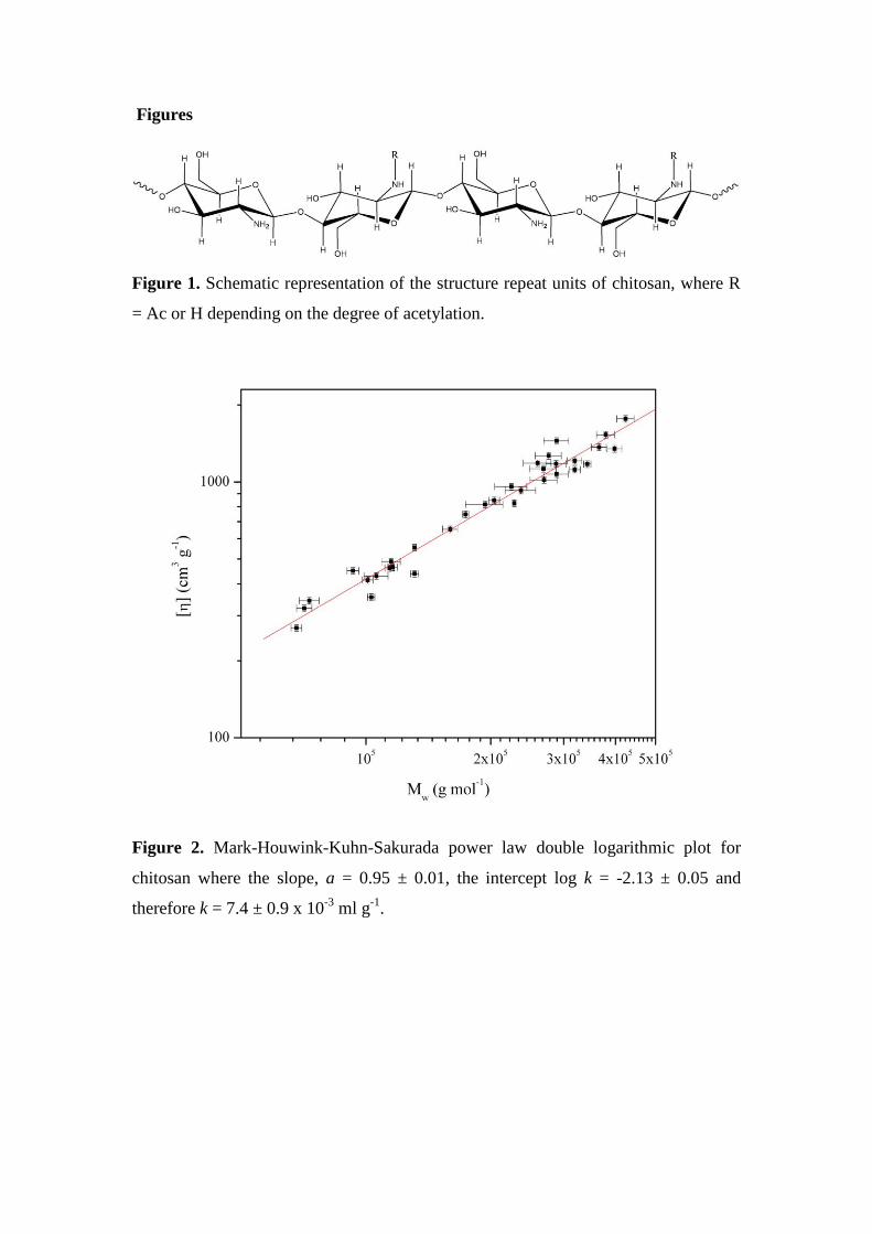
The MHKS exponent (a) is derived using double logarithmic plot of intrinsic

viscosities versus molar mass (Figure 2). In this case we find a value for the

exponent, a, of (0.95 0.01) which is indicative of a rigid rod type molecule and is in

good agreement with previous estimates: 1.0 (Cölfen et al., 2001); 0.96 0.10 (Fee et

al., 2003); 0.90 0.20 (Rinaudo, 2006) and 0.87 0.18 (Kasaai, 2007) the latter two

being the average exponent for 6 and 14 different solvent conditions, respectively.

This procedure assumes a homologous series for the polymers (i.e. they all have

approximately the same conformation type): any departure would reveal itself as

non-linearity of the logarithmic plots. The dominance of hydrodynamic interactions

between chain segments is taken to render insignificant any contribution to the value

of the coefficient though solvent draining effects (Tanford, 1961).

<Figure 2 here>

2. The translational frictional ratio, f/f0

The translational frictional ratio (Tanford, 1961), f/f0 is a parameter which depends on

molar mass, conformation and molecular expansion through hydration effects. It can

be measured experimentally from the sedimentation coefficient and molar mass:

31

,200

,20

,20

0 v3

4

)6(

)v1(

w

A

wwA

ww

M

N

sN

M

f

f (7)

Values in the range 11 – 16 (Table 2) are considerably greater than the theoretical

minimum of 1 and could either be due to long chain elongation or a high degree of

expansion through (aqueous) solvent association, or a combination of both.

3. Wales-van Holde ratio, R = ks/[ ]

Values for the Wales-van Holde ratio (Wales, & van Holde, 1954) in the range 0.39 -

0.73 (Table 2) are obtained which are similar to those found previously 0.26 – 0.73

(Cölfen et al., 2001) and are again consistent with extended structures (Morris, Foster,

& Harding, 2000, Morris, García de al Torre, Ortega, Castile, Smith, & Harding,

2008) but short of the limit for rod (0.15) (Harding, Berth, Ball, Mitchell, & Garcìa de

la Torre, 1991). It has been previously reported that chitosans of higher molar mass

become more compact (Berth et al., 1998) although this is contradicted by the Cölfen

et al (2001) data and also by the new data which both show a decrease in the Wales

van Holde ratio with increase in molar mass, indicating the opposite.

4. Sedimentation Conformation Zoning

The sedimentation conformation zone (Pavlov, Rowe, & Harding, 1997; Pavlov,

Harding, & Rowe, 1999) plot of log [s]/ML versus log ksML enables an estimate of the

“overall” solution conformation of a macromolecule in solution ranging from Zone A

(extra rigid rod) to Zone E (globular or branched). The parameter [s] related to the

sedimentation coefficient by the relation

w

ww

v

ss

,20

,20,200

1 (8)

and ML the mass per unit length 420 g mol-1

nm-1

(Vold, 2004).

The sedimentation conformation zoning (Figure 3 and Table 2) places all three

chitosans as Zone B (rigid rod), although the chitosans 1 and 8 are very close to the

boundary with Zone C (semi-flexible coils).

<Figure 3 and Table 2 here>

5. Combined “Global” Analysis: Multi_HYDFIT

The linear flexibility of polymer chains can also be represented in terms of the

persistence length, Lp of equivalent worm-like chains (Kratky, & Porod, 1949) where

the persistence length is defined as the average projection length along the initial

direction of the polymer chain and for a theoretical perfect random coil Lp = 0 and for

the equivalent extra-rigid rod (Harding, 1997) Lp = ∞, although in practice limits of ~

1 nm for random coils (e.g. pullulan) and 200 nm for an extra-rigid rod (e.g.

schizophyllan) are more appropriate (Tombs, & Harding, 1998).

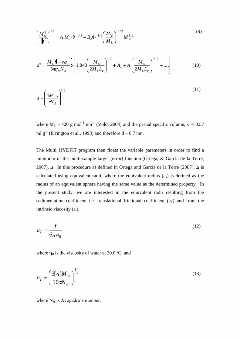
The persistence length and mass per unit length can be estimated using the

Multi_HYDFIT program (Ortega, & García de la Torre, 2007), which considers data

sets of intrinsic viscosities and sedimentation coefficients for different molar mass. It

then performs a minimisation procedure finding the best values of ML and Lp and

chain diameter d satisfying the Bushin-Bohdanecky (Bohdanecky, 1983; Bushin,

Tsvetkov, Lysenko, & Emel’yanov, 1981) and Yamakawa-Fujii (Yamakawa, & Fujii,

1973) equations (equations 9 & 10). Extensive simulations have shown that values

returned for ML and Lp are insensitive to d, so this is usually fixed (Ortega, & García

de la Torre, 2007).

2/1

2/1

3/10

3/10

3/12 2w

L

pL

w MM

LBMA

M (9)

....22

843.13

12/1

32

2/1

0

00

pL

w

pL

w

A

L

LM

MAA

LM

M

N

vMs (10)

2/1

4

A

L

N

vMd

(11)

where ML 420 g mol-1

nm-1

(Vold, 2004) and the partial specific volume, v = 0.57

ml g-1

(Errington et al., 1993) and therefore d 0.7 nm.

The Multi_HYDFIT program then floats the variable parameters in order to find a

minimum of the multi-sample target (error) function (Ortega, & García de la Torre,

2007), In this procedure as defined in Ortega and García de la Torre (2007), is

calculated using equivalent radii, where the equivalent radius (ax) is defined as the

radius of an equivalent sphere having the same value as the determined property. In

the present study, we are interested in the equivalent radii resulting from the

sedimentation coefficient i.e. translational frictional coefficient (aT) and from the

intrinsic viscosity (aI).

06

faT

(12)

where 0 is the viscosity of water at 20.0 ºC, and

31

10

][3

A

wI

N

Ma

(13)

where NA is Avogadro’s number.

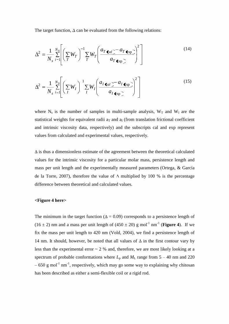
The target function, can be evaluated from the following relations:

sN

i T

TcalT

TT

TT

s a

aaWW

N 1

2

exp

exp1

2 1 (14)

sN

i I

IcalI

II

II

s a

aaWW

N 1

2

exp

exp1

2 1 (15)

where Ns is the number of samples in multi-sample analysis, WT and WI are the

statistical weights for equivalent radii aT and aI (from translation frictional coefficient

and intrinsic viscosity data, respectively) and the subscripts cal and exp represent

values from calculated and experimental values, respectively.

is thus a dimensionless estimate of the agreement between the theoretical calculated

values for the intrinsic viscosity for a particular molar mass, persistence length and

mass per unit length and the experimentally measured parameters (Ortega, & García

de la Torre, 2007), therefore the value of multiplied by 100 % is the percentage

difference between theoretical and calculated values.

<Figure 4 here>

The minimum in the target function ( = 0.09) corresponds to a persistence length of

(16 ± 2) nm and a mass per unit length of (450 ± 20) g mol-1

nm-1

(Figure 4). If we

fix the mass per unit length to 420 nm (Vold, 2004), we find a persistence length of

14 nm. It should, however, be noted that all values of in the first contour vary by

less than the experimental error ~ 2 % and, therefore, we are most likely looking at a

spectrum of probable conformations where Lp and ML range from 5 – 40 nm and 220

– 650 g mol-1

nm-1

, respectively, which may go some way to explaining why chitosan

has been described as either a semi-flexible coil or a rigid rod.

Conclusions

Several previous studies on the solution conformation of chitosan (Table 3)

(Terbojevich et al., 1991; Errington et al., 1993; Cölfen et al., 2001; Fee et al., 2003;

Kasaai, 2007) have suggested a rigid rod conformation whilst others (Rinaudo et al.,

1993; Berth et al., 1998; Brugnerotto et al., 2001; Schatz et al., 2003; Mazeau and

Rinaudo, 2004; Vold, 2004; Larmarque et al., 2005; Velasquez et al., 2008) have

adopted a semi-flexible coil model.

<Table 3 here>

This apparent discrepancy has been in part explained by the new Multi_HYDFIT

approach (Ortega, & Garcia de la Torre, 2007) which has shown that conformation of

chitosan is close to the semi-flexible coil – rigid rod limit and that there are a large

number of possible conformations which could fall in to either of these categories

(Figure 4). This observation would not have been possible with the more traditional

Bushin-Bohdanecky analysis of plotting Mw

213

versus Mw1/2

(Figure 5).

It may therefore be prudent to describe the solution conformation of chitosan as a

semi-flexible rod (or stiff coil).

<Figure 5 here>

References

Berth, G., Dautzenberg, H., & Peter, M. G. (1998). Physico-chemical

characterization of chitosans varying in degree of acetylation. Carbohydrate

Polymers, 36, 205-216.

Bohdanecky, M. (1983). New method for estimating the parameters of the wormlike

chain model from the intrinsic viscosity of stiff-chain polymers. Macromolecules, 16,

1483-1493.

Brugnerotto J., Desbrières J., Roberts G., & Rinaudo M. (2001). Characterization of

chitosan by steric exclusion chromatography. Polymer, 42, 9921–9927.

Bushin, S. V., Tsvetkov, V. N., Lysenko, Y. B., & Emel’yanov, V. N. (1981).

Conformational properties and rigidity of molecules of ladder polyphenylsiloxane in

solutions according the data of sedimentation-diffusion analysis and viscometry.

Vysokomolekulyarnye Soedineniya, A23, 2494-2503.

Cölfen H., Berth, G., & Dautzenberg, H. (2001). Hydrodynamic studies on chitosans

in aqueous solution. Carbohydrate Polymers, 45, 373-383.

Errington, N., Harding, S. E., Vårum, K. M., & Illum, L. (1993). Hydrodynamic

characterisation of chitosans varying in degree of acetylation. International Journal

of Biological Macromolecules, 15, 113-117.

Fee, M., Errington, N., Jumel, K., Illum, L, Smith, A., & Harding, S. E. (2003).

Correlation of SEC/MALLS with ultracentrifuge and viscometric data for chitosans.

European Biophysical Journal, 32, 457-464.

Gralén, N. (1944). Sedimentation and diffusion measurements on cellulose and

cellulose derivatives. PhD Dissertation, University of Uppsala, Sweden.

Harding, S. E. (1997). The Intrinsic viscosity of biological macromolecules. Progress

in measurement, interpretation and application to structure in dilute solution. Progress

in Biophysics and Molecular Biology, 68, 207-262.

Harding, S. E. (2005). Analysis of polysaccharides size, shape and interactions. In D.

J. Scott, S. E. Harding, & A. J. Rowe (Eds.). Analytical Ultracentrifugation

Techniques and Methods (pp. 231-252). Cambridge: Royal Society of Chemistry.

Harding, S. E., Davis, S. S. Deacon, M. P., & Fiebrig, I. (1999). Biopolymer

mucoadhensives. In: Harding, S. E. (Ed.) Biotechnology and Genetic Engineering

Reviews Vol. 16. Intercept: Andover, UK. Pages 41-86.

Harding, S. E., Vårum, K. M., Stokke, B. T., & Smidsrød, O. (1991). Molar mass

determination of polysaccharides. In C. A. White (Ed.). Advances in Carbohydrate

Analysis Vol. 1. JAI Press Limited: Greenwich, USA. Pages 63-144.

Harding, S. E.; Berth, G.; Ball, A.; Mitchell, J. R., & Garcìa de la Torre, J. (1991).

The molar mass distribution and conformation of citrus pectins in solution studied by

hydrodynamics. Carbohydrate Polymers, 168, 1-15.

Kasaai, M. R. (2006). Calculation of Mark–Houwink–Sakurada (MHS) equation

viscometric constants for chitosan in any solvent–temperature system using

experimental reported viscometric constants data. Carbohydrate Polymers, 68, 477-

488.

Kratky, O., & Porod, G. (1949). Röntgenungtersuchung gelöster fadenmoleküle.

Recueil Des Travaux Chimiques Des Pays-Bas, 68, 1106-1109.

Lamarque, G., Lucas, J-M., Viton, C., & Domard, A. (2005). Physicochemical

behavior of homogeneous series of acetylated chitosans in aqueous solution: role of

various structural parameters. Biomacromolecules, 6, 131-142.

Mazeau K., & Rinaudo M. (2004). The prediction of the characteristics of some

polysaccharides from molecular modelling. Comparison with effective behaviour.

Food Hydrocolloids, 18, 885–898.

Morris, G. A.; Foster, T. J., & Harding, S. E. (2000). The effect of degree of

esterification on the hydrodynamic properties of citrus pectin. Food Hydrocolloids,

14, 227-235.

Morris, G. A., García de al Torre, J., Ortega, A., Castile, J., Smith, A., & Harding, S.

E. (2008). Molecular flexibility of citrus pectins by combined sedimentation and

viscosity analysis. Food Hydrocolloids, 22, 1435-1442.

Ortega, A., & García de la Torre, J. (2007). Equivalent radii and ratios of radii from

solution properties as indicators of macromolecular conformation, shape, and

flexibility. Biomacromolecules, 8, 2464-2475.

Pavlov, G. M.; Rowe, A. J., & Harding, S. E. (1997). Conformation zoning of large

molecules using the analytical ultracentrifuge. Trends in Analytical Chemistry, 16,

401-405.

Pavlov, G. M.; Harding, S. E., & Rowe, A. J. (1999). Normalized scaling relations as

a natural classification of linear macromolecules according to size. Progress in

Colloid and Polymer Science, 113, 76-80.

Ralston, G. (1993). Introduction to Analytical Ultracentrifugation (pp 27-28). Palo

Alto: Beckman Instruments Inc.

Rinaudo, M. (2006). Chitin and chitosan: properties and applications. Progress in

Polymer Science, 31, 603-632.

Rinaudo, M., Milas, M., & Le Dung, P. (1993). Characterization of chitosan.

Influence of ionic strength and degree of acetylation on chain expansion.

International Journal of Biological Macromolecules, 15, 281-285.

Rowe, A. J. (1977). The concentration dependence of transport processes: a general

description applicable to the sedimentation, translational diffusion and viscosity

coefficients of macromolecular solutes. Biopolymers, 16, 2595-2611.

Schatz, S. Viton, C., Delair, T. Pichot, C., & Domard, A. (2003). Typical

physicochemical behaviors of chitosan in aqueous solution. Biomacromolecules, 4,

641-648.

Schuck, P. (1998). Sedimentation analysis of noninteracting and self-associating

solutes using numerical solutions to the Lamm equation. Biophysical Journal, 75,

1503-1512.

Schuck, P. (2005). Diffusion-deconvoluted sedimentation coefficient distributions for

the analysis of interacting and non-interacting protein mixtures. In D. J. Scott, S. E.

Harding, & A. J. Rowe (Eds.). Analytical Ultracentrifugation Techniques and

Methods (pp. 26-50). Cambridge: Royal Society of Chemistry.

Solomon, O. F., & Ciutâ, I, Z. (1962). Détermination de la viscosité intrinsèque de

solutions de polymères par une simple détermination de la viscosité. Journal of

Applied Polymer Science, 24, 683-686.

Tanford, C. (1961). Physical Chemistry of Macromolecules. New York: John Wiley

and Sons.

Terbojevich, M. Cosani, A., Conio, G., Marsano, E., & Bianchi, E. (1991). Chitosan:

chain rigidity and mesophase formation. Carbohydrate Research, 209, 251-260.

Tombs, M. P., & Harding, S. E. (1998). Polysaccharide Biotechnology. Taylor

Francis: London, UK. Pages 144-151.

Velásquez, C. L., Albornoz, J. S., & Barrios, E. M. (2008). Viscosimetric studies of

chitosan nitrate and chitosan chlorhydrate in acid free NaCl aqueous solution. E-

Polymers, 014.

Vold, I. M. N. (2004). Periodate Oxidised Chitosans: Structure and Solution

Properties. PhD Dissertation, Norwegian University of Science and Technology,

Trondheim, Norway.

Wales, M., & van Holde, K. E. (1954). The concentration dependence of the

sedimentation constants of flexible macromolecules. Journal of Polymer Science, 14,

81-86.

Yamakawa, H., & Fujii, M. (1973). Translational friction coefficient of wormlike

chains. Macromolecules, 6, 407-415.

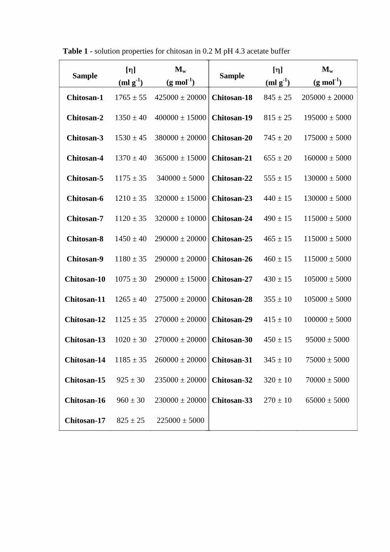
Table 1 - solution properties for chitosan in 0.2 M pH 4.3 acetate buffer

Sample [ ]

(ml g-1

)

Mw

(g mol-1

)

Chitosan-1 1765 ± 55 425000 ± 20000

Chitosan-2 1350 ± 40 400000 ± 15000

Chitosan-3 1530 ± 45 380000 ± 20000

Chitosan-4 1370 ± 40 365000 ± 15000

Chitosan-5 1175 ± 35 340000 ± 5000

Chitosan-6 1210 ± 35 320000 ± 15000

Chitosan-7 1120 ± 35 320000 ± 10000

Chitosan-8 1450 ± 40 290000 ± 20000

Chitosan-9 1180 ± 35 290000 ± 20000

Chitosan-10 1075 ± 30 290000 ± 15000

Chitosan-11 1265 ± 40 275000 ± 20000

Chitosan-12 1125 ± 35 270000 ± 20000

Chitosan-13 1020 ± 30 270000 ± 20000

Chitosan-14 1185 ± 35 260000 ± 20000

Chitosan-15 925 ± 30 235000 ± 20000

Chitosan-16 960 ± 30 230000 ± 20000

Chitosan-17 825 ± 25 225000 ± 5000

Sample [ ]

(ml g-1

)

Mw

(g mol-1

)

Chitosan-18 845 ± 25 205000 ± 20000

Chitosan-19 815 ± 25 195000 ± 5000

Chitosan-20 745 ± 20 175000 ± 5000

Chitosan-21 655 ± 20 160000 ± 5000

Chitosan-22 555 ± 15 130000 ± 5000

Chitosan-23 440 ± 15 130000 ± 5000

Chitosan-24 490 ± 15 115000 ± 5000

Chitosan-25 465 ± 15 115000 ± 5000

Chitosan-26 460 ± 15 115000 ± 5000

Chitosan-27 430 ± 15 105000 ± 5000

Chitosan-28 355 ± 10 105000 ± 5000

Chitosan-29 415 ± 10 100000 ± 5000

Chitosan-30 450 ± 15 95000 ± 5000

Chitosan-31 345 ± 10 75000 ± 5000

Chitosan-32 320 ± 10 70000 ± 5000

Chitosan-33 270 ± 10 65000 ± 5000

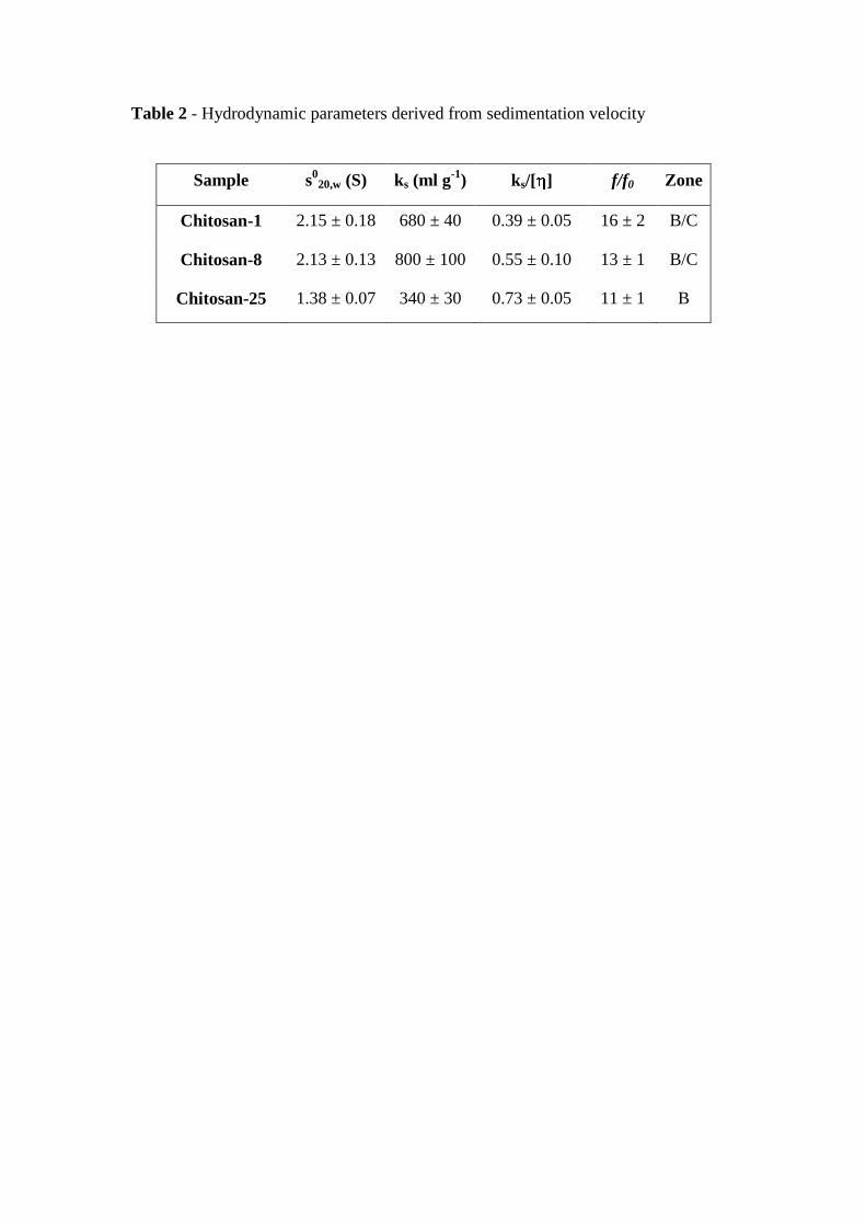
Table 2 - Hydrodynamic parameters derived from sedimentation velocity

Sample s0

20,w (S) ks (ml g-1

) ks/[ ] f/f0 Zone

Chitosan-1 2.15 ± 0.18 680 ± 40 0.39 ± 0.05 16 ± 2 B/C

Chitosan-8 2.13 ± 0.13 800 ± 100 0.55 ± 0.10 13 ± 1 B/C

Chitosan-25 1.38 ± 0.07 340 ± 30 0.73 ± 0.05 11 ± 1 B

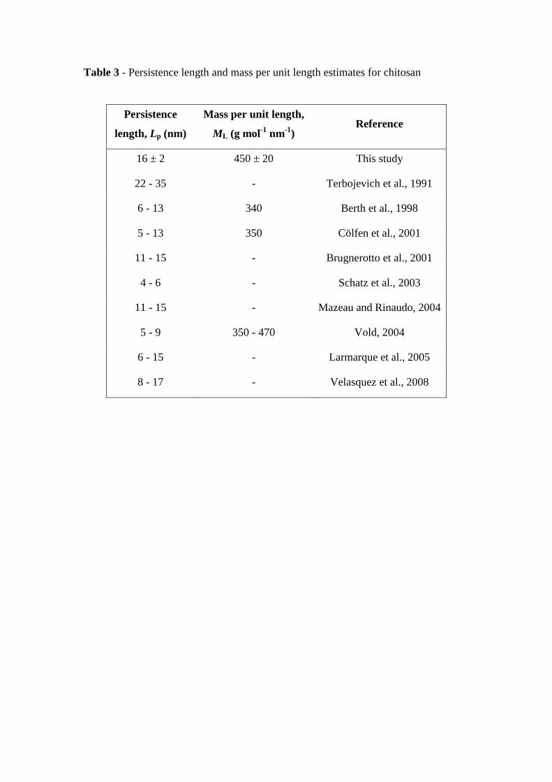
Table 3 - Persistence length and mass per unit length estimates for chitosan

Persistence

length, Lp (nm)

Mass per unit length,

ML (g mol-1

nm-1

) Reference

16 ± 2 450 ± 20 This study

22 - 35 - Terbojevich et al., 1991

6 - 13 340 Berth et al., 1998

5 - 13 350 Cölfen et al., 2001

11 - 15 - Brugnerotto et al., 2001

4 - 6 - Schatz et al., 2003

11 - 15 - Mazeau and Rinaudo, 2004

5 - 9 350 - 470 Vold, 2004

6 - 15 - Larmarque et al., 2005

8 - 17 - Velasquez et al., 2008

Figures

Figure 1. Schematic representation of the structure repeat units of chitosan, where R

= Ac or H depending on the degree of acetylation.

Figure 2. Mark-Houwink-Kuhn-Sakurada power law double logarithmic plot for

chitosan where the slope, a = 0.95 ± 0.01, the intercept log k = -2.13 ± 0.05 and

therefore k = 7.4 ± 0.9 x 10-3

ml g-1

.

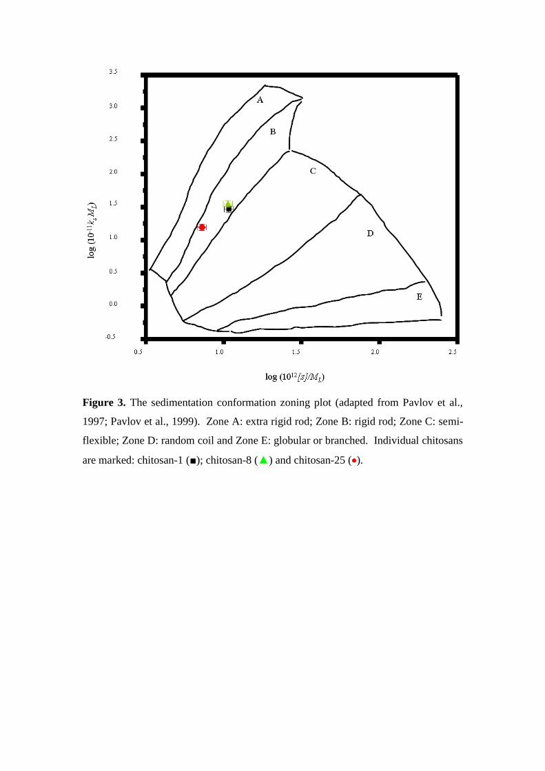
Figure 3. The sedimentation conformation zoning plot (adapted from Pavlov et al.,

1997; Pavlov et al., 1999). Zone A: extra rigid rod; Zone B: rigid rod; Zone C: semi-

flexible; Zone D: random coil and Zone E: globular or branched. Individual chitosans

are marked: chitosan-1 (■); chitosan-8 (▲) and chitosan-25 ( ).

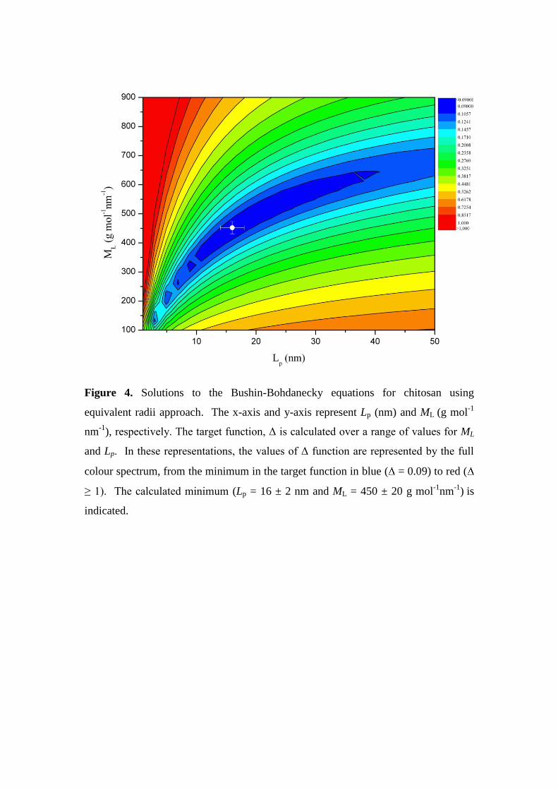
Figure 4. Solutions to the Bushin-Bohdanecky equations for chitosan using

equivalent radii approach. The x-axis and y-axis represent Lp (nm) and ML (g mol-1

nm-1

), respectively. The target function, Δ is calculated over a range of values for ML

and Lp. In these representations, the values of Δ function are represented by the full

colour spectrum, from the minimum in the target function in blue ( = 0.09) to red (

≥ 1). The calculated minimum (Lp = 16 ± 2 nm and ML = 450 ± 20 g mol-1

nm-1

) is

indicated.

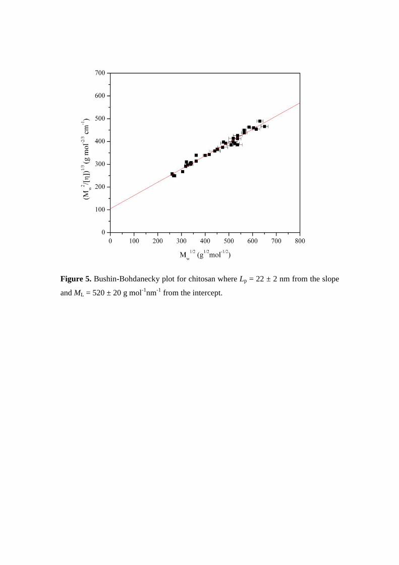
Figure 5. Bushin-Bohdanecky plot for chitosan where Lp = 22 ± 2 nm from the slope

and ML = 520 ± 20 g mol-1

nm-1

from the intercept.