magnetic field of permanent magnets: measurement, modelling,...
TRANSCRIPT
MAGNETIC FIELD OF PERMANENT MAGNETS: MEASUREMENT, MODELLING, VIZUALIZATION
T. Mikolanda, M. Košek, A. Richter
Technical University of Liberec, Studentská 2, 46117, Liberec
Abstract
MATLAB language is a quite general and high power language. Thanks to its complexity, simplicity and universality it was used anywhere in the complete study of permanent magnet force action. Main use is the control of fully automated apparatus, data acquisition and processing, numerical integration according to the models of permanent magnets, visualization of results, simulation of the dynamic effects, fast calculations by the sue of cluster, etc. Fully automated apparatus made possible the measurement of magnetic field with high accuracy. Relatively simple models of magnets, based on numerical integration, were in surprisingly good agreement with experiment. Calculated and measured magnetic field was visualized by parametric graphs, but other more descriptive methods as flux density vectors or lines were also realized. In order to speed numerical integration, the cluster is in preparation.
Introduction The magnetic force in the form of magnetic coupling is used in many technical and scientific
applications, especially for contact-less force, momentum, contact-less shaft bearing and levitation, for instance. The survey of magnetic coupling methods and applications can be found in literature [1]. In order to achieve optimal system design, theoretical models of magnetic field are often used. In the literature model based on non-existing magnetic charges is often used in a very formal analogy with electrostatic field [2]. But two other models are possible: the model of coupled currents and the model of elementary magnetic dipoles. However the last model is complicated both theoretically and numerically.
In the magnetic field modeling we apply the method of coupled currents that appears to be universal and efficient one. In order to verify models, a precise magnetic field measurement is necessary. Therefore, the accurate measurement of magnetic field is the second topic of the paper. The paper contains also the visualization of results in very effective forms.
1 Theory Permanent magnet model uses the magnet shape, its geometrical parameters and material
property, the distribution of magnetization. They fully describe its magnetic properties ana the magnetization is the source of magnetic filed. In principle, there are two basic procedures for the computation of magnetic field: the differential and integral ones. The differential approach is based on Poisson equation for vector potential, supposes the application of FEM, therefore it is not suitable for our case. The integral approach requires the use of models, if we do not consider the use of elementary dipoles.
As it was explained in Introduction, from the possible models, we prefer the use of the coupled surface and volume current model. Then the Biot-Savart Law, which requires only the numerical integration, can be applied.
Before the start of key formulae presentation, the coordinate convention will be mentioned. There are two types of coordinates or position vectors: material and field ones. Material position vector has zero indexes, , for instance, and it denotes the position of elementary dipole, current element etc. Field vector without any index, for instance, defines the point, at which the field quantity, as magnetic flux density, is calculated.
This abbreviation is often used for difference of these vectors

(1)
The distance between source (material quantity position) and response (field quantity position) is denoted by
(2)
Magnetic properties of permanent magnet are described by the magnetization M which is the density of magnetic dipole momentum. The method of coupled currents is based on the following fact. In the literature [3], for instance, it is shown that the same field can be produced by suitable fictive currents flowing in the volume and on the surface of the permanent magnet. The currents are termed coupled currents in order to distinguish them from real free currents. Both the currents are derived from the magnetization. The volume coupled current is given by formula
(5)
For the surface current the following formula is derived
(6)
In the formula the unit vector n is the vector normal to the permanent magnet surface and its direction is from the inner side of the surface with index 1 to the outer one of index 2. Since magnetization outside the permanent magnet is zero, only inner part M1 very close to the surface take a place. It is equal to the magnetization M, M1 = M. While the free currents can be changed by many means according to requirements of experiment, the coupled current can be changed only by the change of magnetization.
The magnetic field produced by coupled currents is the same as the field given by free currents. In both cases the Biot-Savart Law can be used [3]. The flux density at point with field vector r produced by volume currents in volume Vo is given by formula
(7)
The integration in the volume Vo is described symbolically as (Vo). In real calculation the sample lengths or similar parameters in suitable 3D coordinate system are the integration limits.
The same procedure can be used for surface currents. The flux density at point with field vector r produced by surface currents flowing on the sample surface So is given by formula
(8)
The integration over the sample surface So is denoted symbolically as (So). In real calculation the suitable limits derived from sample shape should be used
2 Experiment In order to verify proposed models an accurate measurement of magnetic field is necessary.
Therefore, an apparatus for automated and precise 2D magnetic field measurement was realized. In this chapter we describe the realized apparatus and we also mention its accuracy and reduction of several errors.
Apparatus In order to achieve precise 3D magnetic field measurements we have realized two independent
perpendicular positioning systems of Hall probe for its location in horizontal plane. Vertical plane is actually shifted manually. For accurate vertical position the precise spread plates are used. The measurement is fully automated and controlled by the computer, detailed description follows.
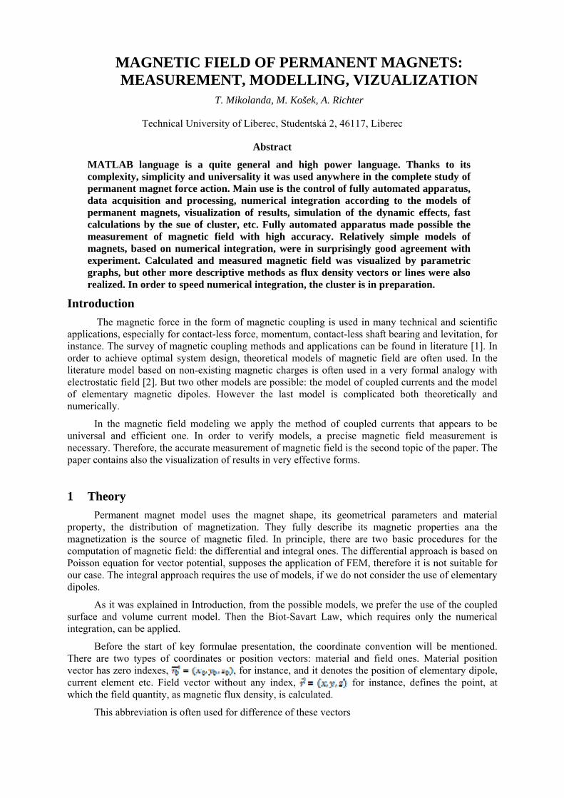
Block scheme of realized measurement apparatus is shown at Fig. 2. The concept of such a system can be divided to several parts, mechanical part, electronic and measurement part and a control one. Photo of apparatus is shown at Fig. 1.
Fig. 1: Measurement apparatus photo.
Fig. 2: Measurement apparatus block scheme
Mechanical part consists of two linear non-pneumatic shafts made by FESTO, which are connected together with modular bridge. That connection is perpendicular and makes the system tough and suppresses shafts torsion as well. Bottom shaft is chocked up along the whole length to eliminate axial twist. Due to this modular construction the system realizes very good balance and parallelism at any possible position. The apparatus was put under the test with good results. Vertical parallelism measured at the most distant places at x-axis (top one) differs only by about 20 μm which corresponds to thickness of typical list of paper. Measured deviation is the same for various positions of y-axis (bottom one).
Linear shafts are driven by step motors with small step. The junction between shaft and step motor is made by soft conjunction. The positioning part of apparatus exhibits the uncertainty of location of 40 μm.
M

Each step motor is driven by separate step motor controller SOFCON PKM02. These units are connected to control logic processor which translates supervising commands sent from control PC via TIA/EIA 232 or USB to electrical signals. Control unit utilizes reduced set of standard SCPI commands together with system specialized ones which are in SCPI compliance.
For the measurement of magnetic field we have used 3D Hall probe ELIDIS TMHSDMP1. Probe output is connected to NI DAQ 6211 ADC. Sampled data are transferred into PC via USB interface, as shown at Fig. 2, where they are processed and saved.
Measurement, as well as position control, is done by user program at PC side. We use the MATLAB environment due to its simplicity and abilities of easy data processing. We have prepared fully object oriented classes for position and motion control, data transfer via available interfaces and for data processing. It allows motion history, reverting of improper steps, home setting, and independent position and speed parameters for each axis and online data visualization, for example.
Error reduction Two types of error exist: error in the probe position and in the magnetic field value read from
the probe. By the careful evaluation of errors from all the mechanical parts, the probe position error was estimated to be about 40 µm. Practically, its value is not so important since the active part of probe has finite dimensions of about 1 mm and the probe integrating effect take a place. The practical accuracy is about 0.5 mm.
Main source of errors in the probe electrical output are many types of electrical noise. One of the typical uncertainties is in the form of the superposition of 50 Hz net noise to measured signal in time. Such disturbance can be eliminated in several ways. One is averaging during one period; it is fast but needs complicated SW. Apart from that it puts emphasize on exact phase agreement and sampling frequency. Noise can be reduced also by averaging during a lot of periods, which is slow, but does not put such emphasis on exact parameters; necessary SW is simple. Again the MATLAB was used for the realization of averaging.
Fig. 3: Net noise reduction by averaging, linear scale for noise reduction.
Results from exact analytical equations for average value of noise are in Fig. 3 with linear scale and in Fig. 4 containing a logarithmic scale. The calculations were made by MATLAB. The noise suppression value of 40 dB (or linearly to 1 %) is given by horizontal line. It follows from both the figures that for such net noise suppression total 32 periods must be averaged in the worst case. This number of periods is in a well agreement with experiment.
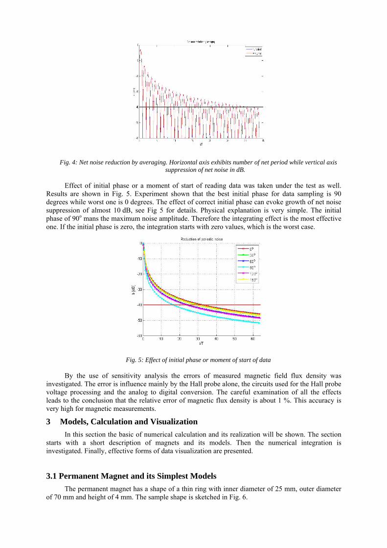
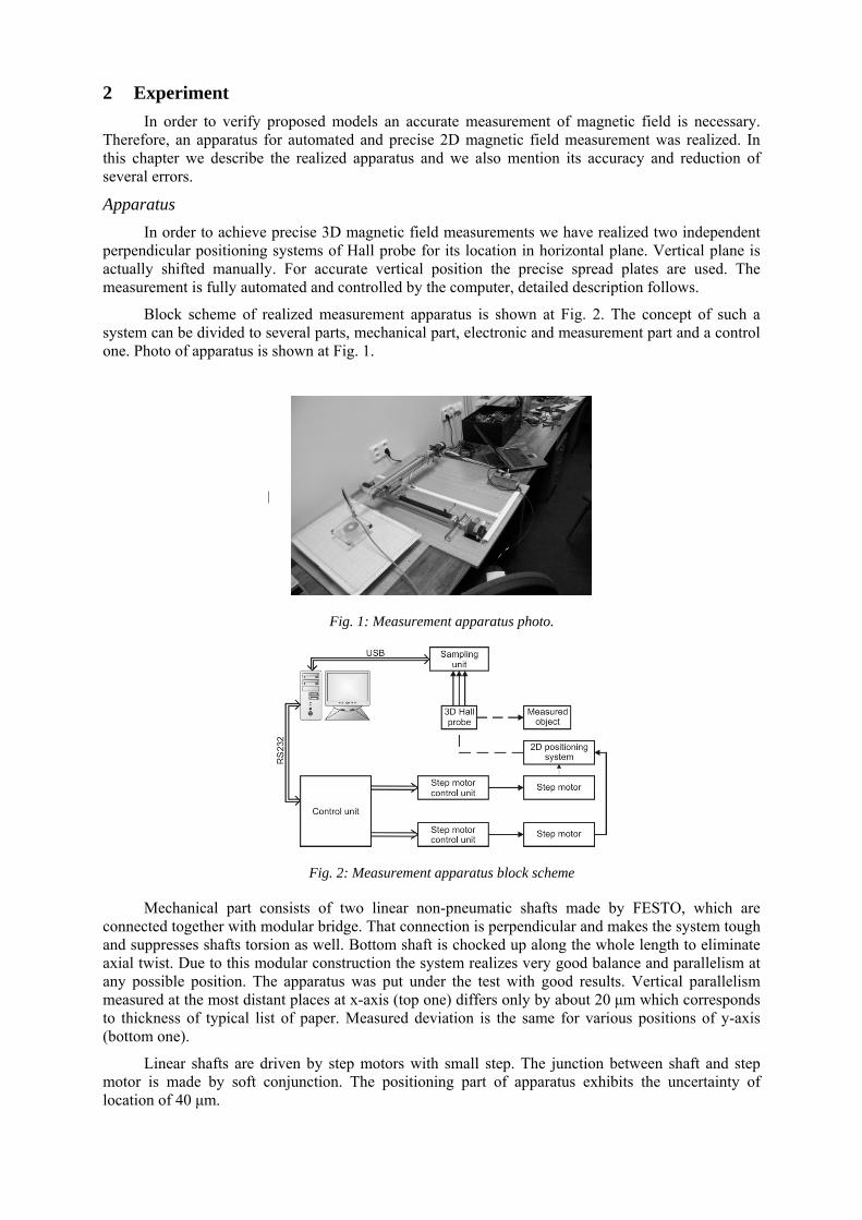
Fig. 4: Net noise reduction by averaging. Horizontal axis exhibits number of net period while vertical axis suppression of net noise in dB.
Effect of initial phase or a moment of start of reading data was taken under the test as well. Results are shown in Fig. 5. Experiment shown that the best initial phase for data sampling is 90 degrees while worst one is 0 degrees. The effect of correct initial phase can evoke growth of net noise suppression of almost 10 dB, see Fig 5 for details. Physical explanation is very simple. The initial phase of 90o mans the maximum noise amplitude. Therefore the integrating effect is the most effective one. If the initial phase is zero, the integration starts with zero values, which is the worst case.
Fig. 5: Effect of initial phase or moment of start of data
By the use of sensitivity analysis the errors of measured magnetic field flux density was investigated. The error is influence mainly by the Hall probe alone, the circuits used for the Hall probe voltage processing and the analog to digital conversion. The careful examination of all the effects leads to the conclusion that the relative error of magnetic flux density is about 1 %. This accuracy is very high for magnetic measurements.
3 Models, Calculation and Visualization In this section the basic of numerical calculation and its realization will be shown. The section
starts with a short description of magnets and its models. Then the numerical integration is investigated. Finally, effective forms of data visualization are presented.
3.1 Permanent Magnet and its Simplest Models The permanent magnet has a shape of a thin ring with inner diameter of 25 mm, outer diameter
of 70 mm and height of 4 mm. The sample shape is sketched in Fig. 6.
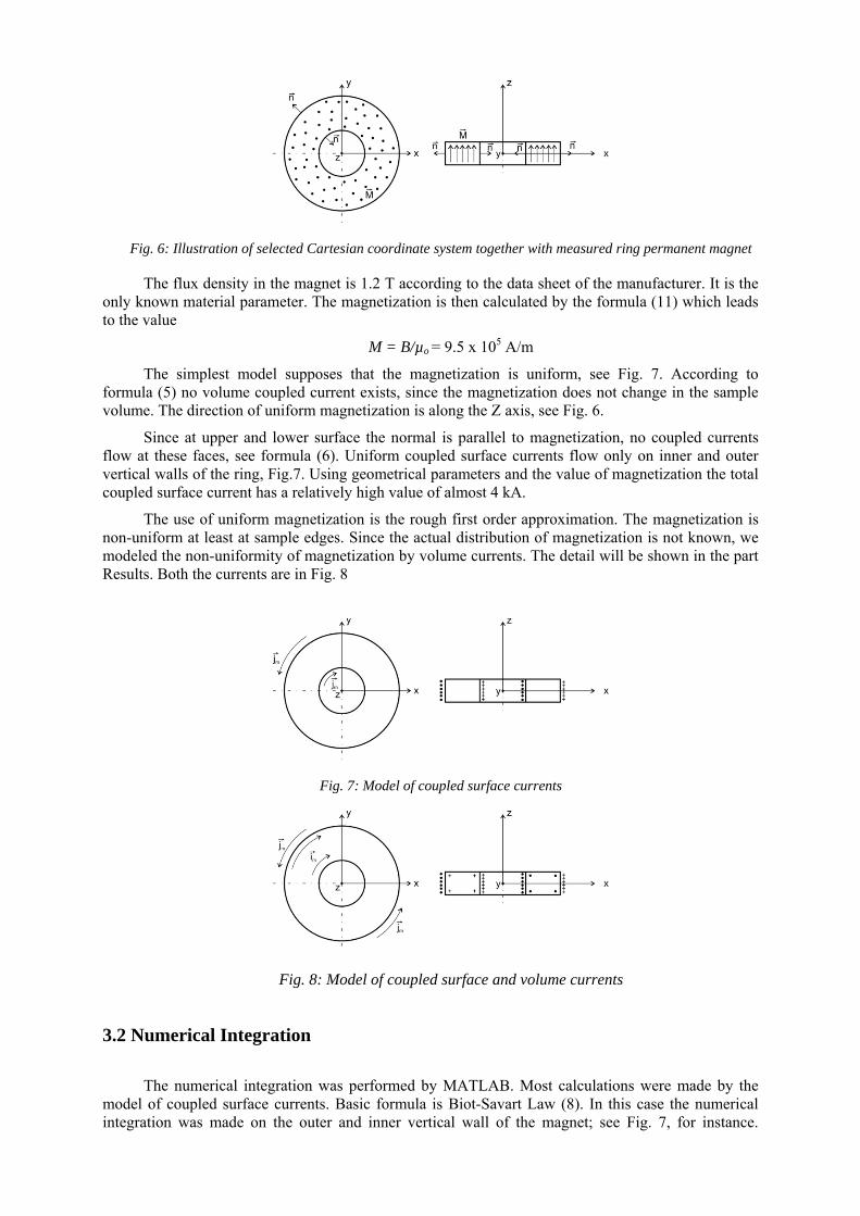
Fig. 6: Illustration of selected Cartesian coordinate system together with measured ring permanent magnet
The flux density in the magnet is 1.2 T according to the data sheet of the manufacturer. It is the only known material parameter. The magnetization is then calculated by the formula (11) which leads to the value
M = B/µo = 9.5 x 10⁵ A/m
The simplest model supposes that the magnetization is uniform, see Fig. 7. According to formula (5) no volume coupled current exists, since the magnetization does not change in the sample volume. The direction of uniform magnetization is along the Z axis, see Fig. 6.
Since at upper and lower surface the normal is parallel to magnetization, no coupled currents flow at these faces, see formula (6). Uniform coupled surface currents flow only on inner and outer vertical walls of the ring, Fig.7. Using geometrical parameters and the value of magnetization the total coupled surface current has a relatively high value of almost 4 kA.
The use of uniform magnetization is the rough first order approximation. The magnetization is non-uniform at least at sample edges. Since the actual distribution of magnetization is not known, we modeled the non-uniformity of magnetization by volume currents. The detail will be shown in the part Results. Both the currents are in Fig. 8
Fig. 7: Model of coupled surface currents
Fig. 8: Model of coupled surface and volume currents
3.2 Numerical Integration
The numerical integration was performed by MATLAB. Most calculations were made by the model of coupled surface currents. Basic formula is Biot-Savart Law (8). In this case the numerical integration was made on the outer and inner vertical wall of the magnet; see Fig. 7, for instance.
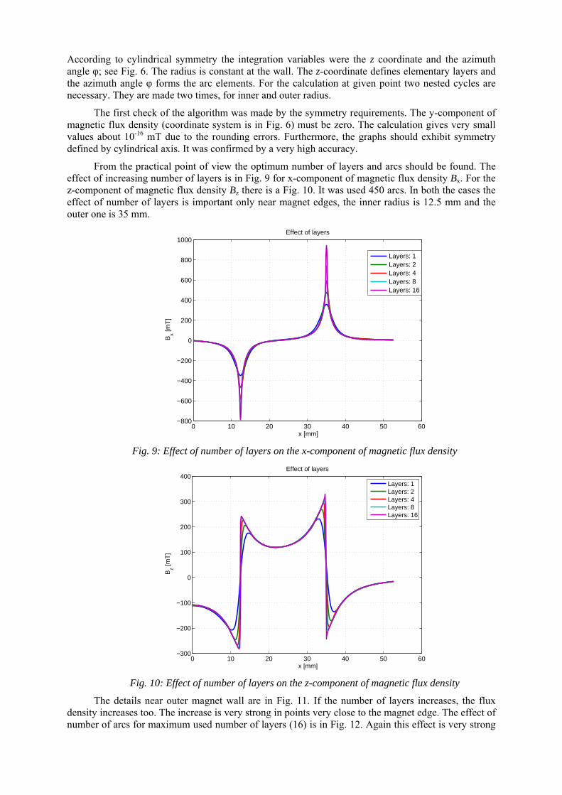
According to cylindrical symmetry the integration variables were the z coordinate and the azimuth angle φ; see Fig. 6. The radius is constant at the wall. The z-coordinate defines elementary layers and the azimuth angle φ forms the arc elements. For the calculation at given point two nested cycles are necessary. They are made two times, for inner and outer radius.
The first check of the algorithm was made by the symmetry requirements. The y-component of magnetic flux density (coordinate system is in Fig. 6) must be zero. The calculation gives very small values about 10-16 mT due to the rounding errors. Furthermore, the graphs should exhibit symmetry defined by cylindrical axis. It was confirmed by a very high accuracy.
From the practical point of view the optimum number of layers and arcs should be found. The effect of increasing number of layers is in Fig. 9 for x-component of magnetic flux density Bx. For the z-component of magnetic flux density Bz there is a Fig. 10. It was used 450 arcs. In both the cases the effect of number of layers is important only near magnet edges, the inner radius is 12.5 mm and the outer one is 35 mm.
0 10 20 30 40 50 60−800
−600
−400
−200
0
200
400
600
800
1000
x [mm]
Bx [m
T]
Effect of layers
Layers: 1Layers: 2Layers: 4Layers: 8Layers: 16
Fig. 9: Effect of number of layers on the x-component of magnetic flux density
0 10 20 30 40 50 60−300
−200
−100
0
100
200
300
400
x [mm]
Bz [m
T]
Effect of layers
Layers: 1Layers: 2Layers: 4Layers: 8Layers: 16
Fig. 10: Effect of number of layers on the z-component of magnetic flux density
The details near outer magnet wall are in Fig. 11. If the number of layers increases, the flux density increases too. The increase is very strong in points very close to the magnet edge. The effect of number of arcs for maximum used number of layers (16) is in Fig. 12. Again this effect is very strong
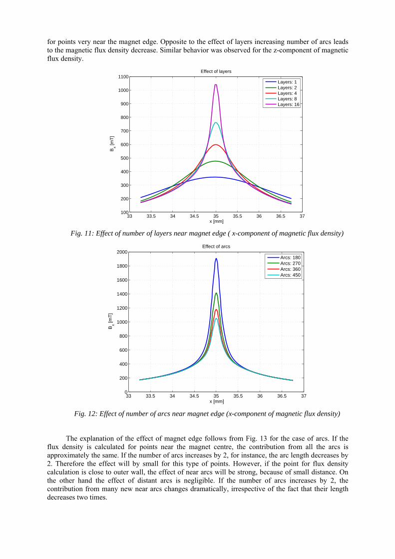
for points very near the magnet edge. Opposite to the effect of layers increasing number of arcs leads to the magnetic flux density decrease. Similar behavior was observed for the z-component of magnetic flux density.
33 33.5 34 34.5 35 35.5 36 36.5 37100
200
300
400
500
600
700
800
900
1000
1100
x [mm]
Bx [m
T]
Effect of layers
Layers: 1Layers: 2Layers: 4Layers: 8Layers: 16
Fig. 11: Effect of number of layers near magnet edge ( x-component of magnetic flux density)
33 33.5 34 34.5 35 35.5 36 36.5 370
200
400
600
800
1000
1200
1400
1600
1800
2000
x [mm]
Bx [m
T]
Effect of arcs
Arcs: 180Arcs: 270Arcs: 360Arcs: 450
Fig. 12: Effect of number of arcs near magnet edge (x-component of magnetic flux density)
The explanation of the effect of magnet edge follows from Fig. 13 for the case of arcs. If the flux density is calculated for points near the magnet centre, the contribution from all the arcs is approximately the same. If the number of arcs increases by 2, for instance, the arc length decreases by 2. Therefore the effect will by small for this type of points. However, if the point for flux density calculation is close to outer wall, the effect of near arcs will be strong, because of small distance. On the other hand the effect of distant arcs is negligible. If the number of arcs increases by 2, the contribution from many new near arcs changes dramatically, irrespective of the fact that their length decreases two times.
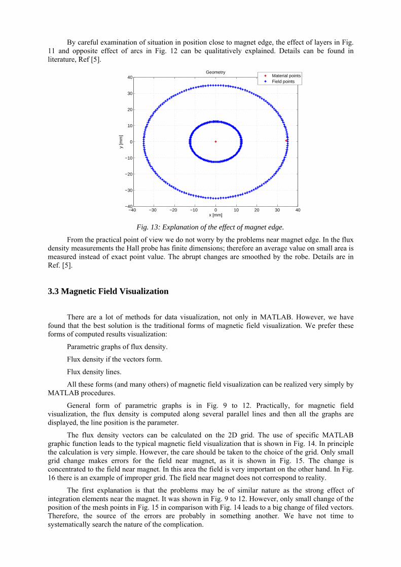
By careful examination of situation in position close to magnet edge, the effect of layers in Fig. 11 and opposite effect of arcs in Fig. 12 can be qualitatively explained. Details can be found in literature, Ref [5].
−40 −30 −20 −10 0 10 20 30 40−40
−30
−20
−10
0
10
20
30
40
x [mm]
y [m
m]
Geometry
Material pointsField points
Fig. 13: Explanation of the effect of magnet edge.
From the practical point of view we do not worry by the problems near magnet edge. In the flux density measurements the Hall probe has finite dimensions; therefore an average value on small area is measured instead of exact point value. The abrupt changes are smoothed by the robe. Details are in Ref. [5].
3.3 Magnetic Field Visualization
There are a lot of methods for data visualization, not only in MATLAB. However, we have found that the best solution is the traditional forms of magnetic field visualization. We prefer these forms of computed results visualization:
Parametric graphs of flux density.
Flux density if the vectors form.
Flux density lines.
All these forms (and many others) of magnetic field visualization can be realized very simply by MATLAB procedures.
General form of parametric graphs is in Fig. 9 to 12. Practically, for magnetic field visualization, the flux density is computed along several parallel lines and then all the graphs are displayed, the line position is the parameter.
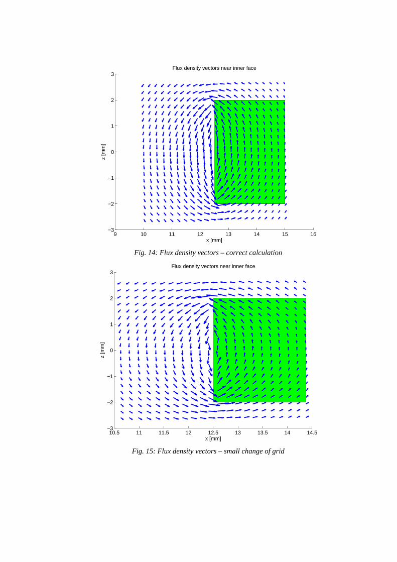
The flux density vectors can be calculated on the 2D grid. The use of specific MATLAB graphic function leads to the typical magnetic field visualization that is shown in Fig. 14. In principle the calculation is very simple. However, the care should be taken to the choice of the grid. Only small grid change makes errors for the field near magnet, as it is shown in Fig. 15. The change is concentrated to the field near magnet. In this area the field is very important on the other hand. In Fig. 16 there is an example of improper grid. The field near magnet does not correspond to reality.
The first explanation is that the problems may be of similar nature as the strong effect of integration elements near the magnet. It was shown in Fig. 9 to 12. However, only small change of the position of the mesh points in Fig. 15 in comparison with Fig. 14 leads to a big change of filed vectors. Therefore, the source of the errors are probably in something another. We have not time to systematically search the nature of the complication.
9 10 11 12 13 14 15 16−3
−2
−1
0
1
2
3
x [mm]
z [m
m]
Flux density vectors near inner face
Fig. 14: Flux density vectors – correct calculation
10.5 11 11.5 12 12.5 13 13.5 14 14.5−3
−2
−1
0
1
2
3
x [mm]
z [m
m]
Flux density vectors near inner face
Fig. 15: Flux density vectors – small change of grid
10 10.5 11 11.5 12 12.5 13 13.5 14 14.5 15−1
−0.5
0
0.5
1
1.5
2
2.5
3
x [mm]
z [m
m]
Flux density vectors near edge
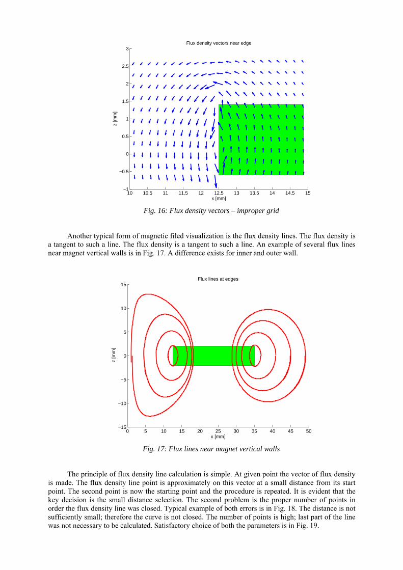
Fig. 16: Flux density vectors – improper grid
Another typical form of magnetic filed visualization is the flux density lines. The flux density is a tangent to such a line. The flux density is a tangent to such a line. An example of several flux lines near magnet vertical walls is in Fig. 17. A difference exists for inner and outer wall.
0 5 10 15 20 25 30 35 40 45 50−15
−10
−5
0
5
10
15
x [mm]
z [m
m]
Flux lines at edges
Fig. 17: Flux lines near magnet vertical walls
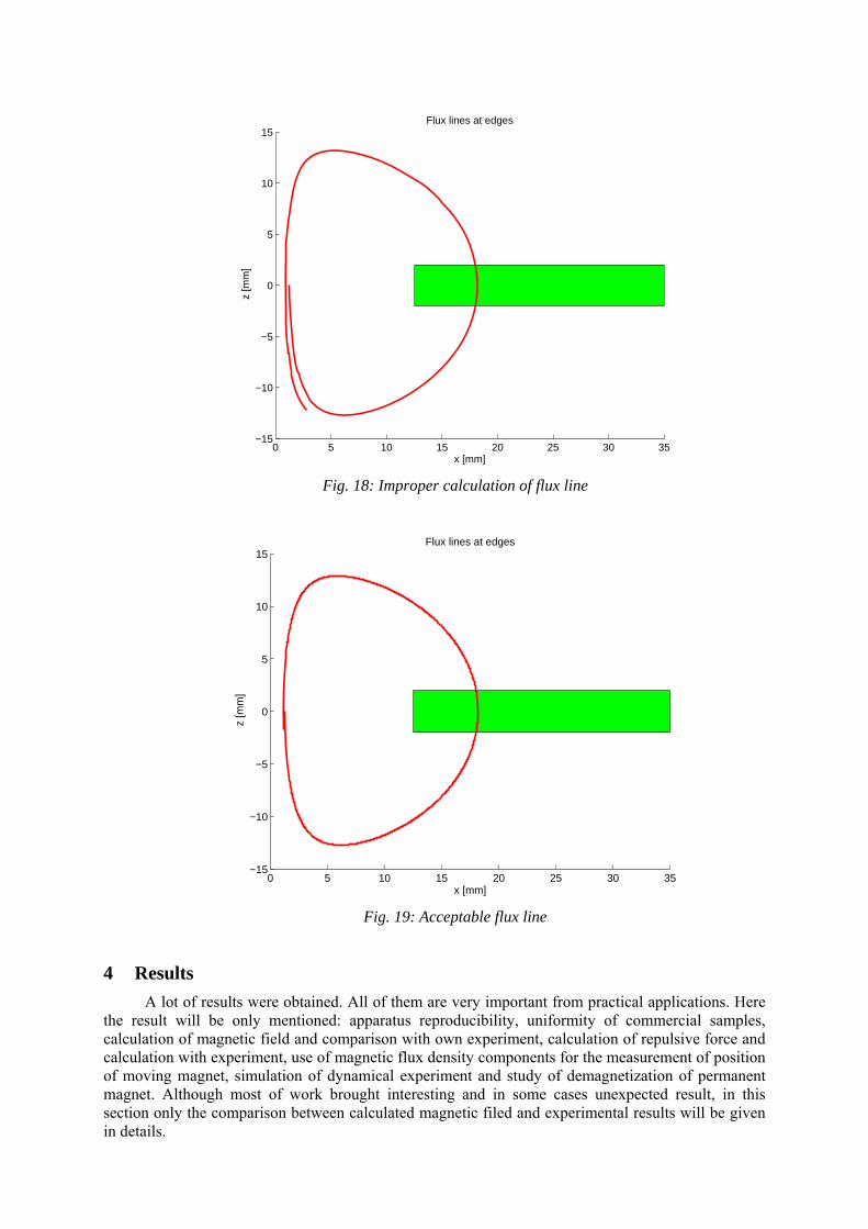
The principle of flux density line calculation is simple. At given point the vector of flux density is made. The flux density line point is approximately on this vector at a small distance from its start point. The second point is now the starting point and the procedure is repeated. It is evident that the key decision is the small distance selection. The second problem is the proper number of points in order the flux density line was closed. Typical example of both errors is in Fig. 18. The distance is not sufficiently small; therefore the curve is not closed. The number of points is high; last part of the line was not necessary to be calculated. Satisfactory choice of both the parameters is in Fig. 19.
0 5 10 15 20 25 30 35−15
−10
−5
0
5
10
15
x [mm]
z [m
m]
Flux lines at edges
Fig. 18: Improper calculation of flux line
0 5 10 15 20 25 30 35−15
−10
−5
0
5
10
15
x [mm]
z [m
m]
Flux lines at edges
Fig. 19: Acceptable flux line
4 Results A lot of results were obtained. All of them are very important from practical applications. Here
the result will be only mentioned: apparatus reproducibility, uniformity of commercial samples, calculation of magnetic field and comparison with own experiment, calculation of repulsive force and calculation with experiment, use of magnetic flux density components for the measurement of position of moving magnet, simulation of dynamical experiment and study of demagnetization of permanent magnet. Although most of work brought interesting and in some cases unexpected result, in this section only the comparison between calculated magnetic filed and experimental results will be given in details.
4.1 Comparison between Theory and Experiment The surprising result from performed measurements was that we have measured nonzero
component By, although by symmetry this component should have zero values. The measured values were much higher than experimental errors.
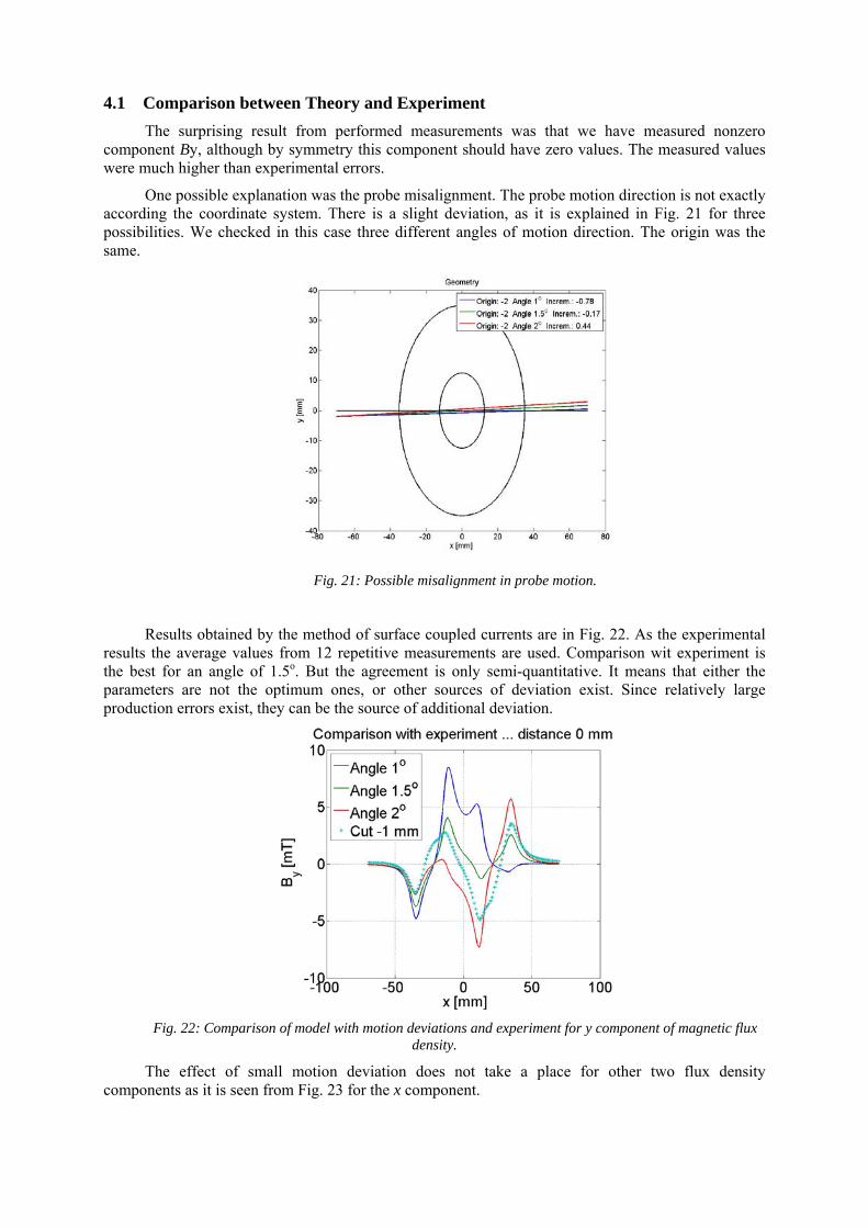
One possible explanation was the probe misalignment. The probe motion direction is not exactly according the coordinate system. There is a slight deviation, as it is explained in Fig. 21 for three possibilities. We checked in this case three different angles of motion direction. The origin was the same.
Fig. 21: Possible misalignment in probe motion.
Results obtained by the method of surface coupled currents are in Fig. 22. As the experimental results the average values from 12 repetitive measurements are used. Comparison wit experiment is the best for an angle of 1.5o. But the agreement is only semi-quantitative. It means that either the parameters are not the optimum ones, or other sources of deviation exist. Since relatively large production errors exist, they can be the source of additional deviation.
Fig. 22: Comparison of model with motion deviations and experiment for y component of magnetic flux
density.
The effect of small motion deviation does not take a place for other two flux density components as it is seen from Fig. 23 for the x component.
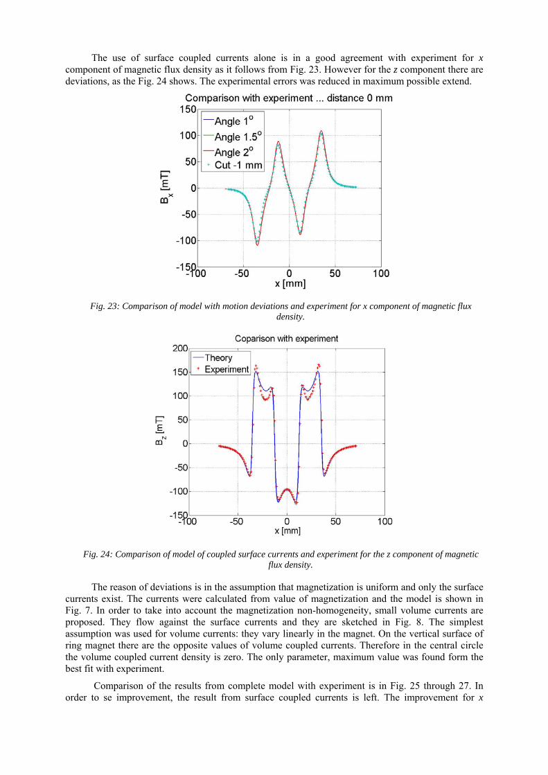
The use of surface coupled currents alone is in a good agreement with experiment for x component of magnetic flux density as it follows from Fig. 23. However for the z component there are deviations, as the Fig. 24 shows. The experimental errors was reduced in maximum possible extend.
Fig. 23: Comparison of model with motion deviations and experiment for x component of magnetic flux density.
Fig. 24: Comparison of model of coupled surface currents and experiment for the z component of magnetic flux density.
The reason of deviations is in the assumption that magnetization is uniform and only the surface currents exist. The currents were calculated from value of magnetization and the model is shown in Fig. 7. In order to take into account the magnetization non-homogeneity, small volume currents are proposed. They flow against the surface currents and they are sketched in Fig. 8. The simplest assumption was used for volume currents: they vary linearly in the magnet. On the vertical surface of ring magnet there are the opposite values of volume coupled currents. Therefore in the central circle the volume coupled current density is zero. The only parameter, maximum value was found form the best fit with experiment.
Comparison of the results from complete model with experiment is in Fig. 25 through 27. In order to se improvement, the result from surface coupled currents is left. The improvement for x
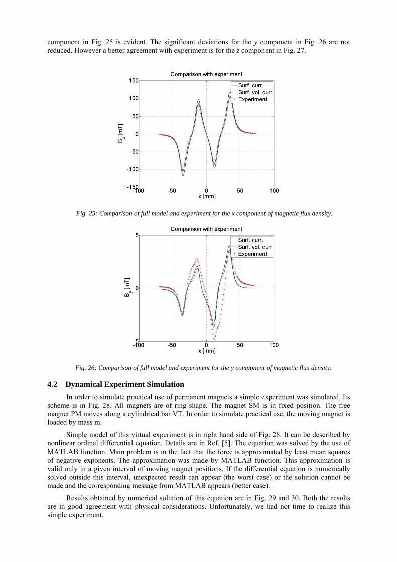
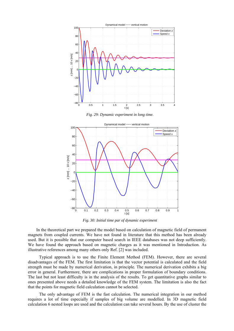
component in Fig. 25 is evident. The significant deviations for the y component in Fig. 26 are not reduced. However a better agreement with experiment is for the z component in Fig. 27.
Fig. 25: Comparison of full model and experiment for the x component of magnetic flux density.
Fig. 26: Comparison of full model and experiment for the y component of magnetic flux density.
4.2 Dynamical Experiment Simulation In order to simulate practical use of permanent magnets a simple experiment was simulated. Its
scheme is in Fig. 28. All magnets are of ring shape. The magnet SM is in fixed position. The free magnet PM moves along a cylindrical bar VT. In order to simulate practical use, the moving magnet is loaded by mass m.
Simple model of this virtual experiment is in right hand side of Fig. 28. It can be described by nonlinear ordinal differential equation. Details are in Ref. [5]. The equation was solved by the use of MATLAB function. Main problem is in the fact that the force is approximated by least mean squares of negative exponents. The approximation was made by MATLAB function. This approximation is valid only in a given interval of moving magnet positions. If the differential equation is numerically solved outside this interval, unexpected result can appear (the worst case) or the solution cannot be made and the corresponding message from MATLAB appears (better case).
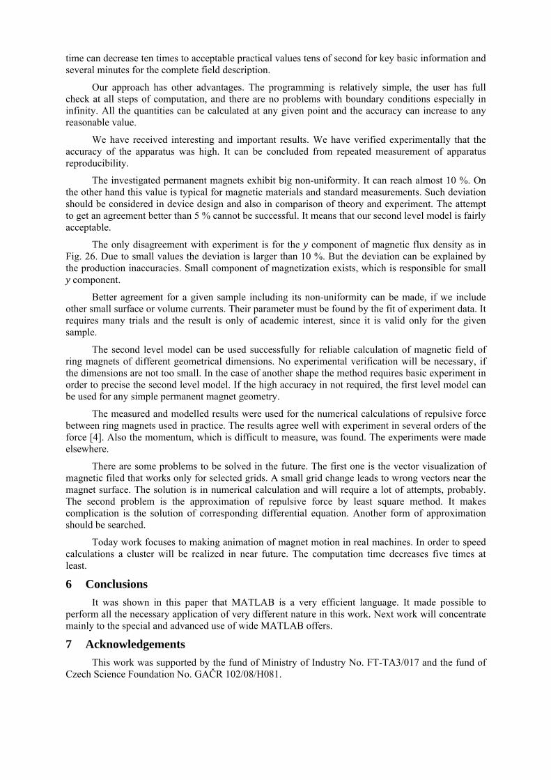
Results obtained by numerical solution of this equation are in Fig. 29 and 30. Both the results are in good agreement with physical considerations. Unfortunately, we had not time to realize this simple experiment.
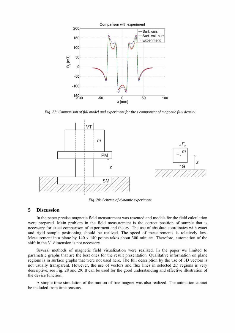
Fig. 27: Comparison of full model and experiment for the z component of magnetic flux density.
Fig. 28: Scheme of dynamic experiment.
5 Discussion In the paper precise magnetic field measurement was resented and models for the field calculation
were prepared. Main problem in the field measurement is the correct position of sample that is necessary for exact comparison of experiment and theory. The use of absolute coordinates with exact and rigid sample positioning should be realized. The speed of measurements is relatively low. Measurement in a plane by 140 x 140 points takes about 300 minutes. Therefore, automation of the shift in the 3rd dimension is not necessary.
Several methods of magnetic field visualization were realized. In the paper we limited to parametric graphs that are the best ones for the result presentation. Qualitative information on plane regions is in surface graphs that were not used here. The full description by the use of 3D vectors is not usually transparent. However, the use of vectors and flux lines in selected 2D regions is very descriptive, see Fig. 28 and 29. It can be used for the good understanding and effective illustration of the device function.
A simple time simulation of the motion of free magnet was also realized. The animation cannot be included from time reasons.
0 0.5 1 1.5 2 2.5 3 3.5 4−80
−60
−40
−20
0
20
40
60
80
100
t [s]
z [m
m] .
.. 10
v [m
/s]
Dynamical model −−− vertical motion
Deviation zSpeed v
Fig. 29: Dynamic experiment in long time.
0 0.1 0.2 0.3 0.4 0.5 0.6 0.7 0.8 0.9 1−80
−60
−40
−20
0
20
40
60
80
100
t [s]
z [m
m] .
.. 10
v [m
/s]
Dynamical model −−− vertical motion
Deviation zSpeed v
Fig. 30: Initial time par of dynamic experiment
In the theoretical part we prepared the model based on calculation of magnetic field of permanent magnets from coupled currents. We have not found in literature that this method has been already used. But it is possible that our computer based search in IEEE databases was not deep sufficiently. We have found the approach based on magnetic charges as it was mentioned in Introduction. As illustrative references among many others only Ref. [2] was included.
Typical approach is to use the Finite Element Method (FEM). However, there are several disadvantages of the FEM. The first limitation is that the vector potential is calculated and the field strength must be made by numerical derivation, in principle. The numerical derivation exhibits a big error in general. Furthermore, there are complications in proper formulation of boundary conditions. The last but not least difficulty is in the analysis of the results. To get quantitative graphs similar to ones presented above needs a detailed knowledge of the FEM system. The limitation is also the fact that the points for magnetic field calculation cannot be selected.
The only advantage of FEM is the fast calculation. The numerical integration in our method requires a lot of time especially if samples of big volume are modelled. In 3D magnetic field calculation 6 nested loops are used and the calculation can take several hours. By the use of cluster the
time can decrease ten times to acceptable practical values tens of second for key basic information and several minutes for the complete field description.
Our approach has other advantages. The programming is relatively simple, the user has full check at all steps of computation, and there are no problems with boundary conditions especially in infinity. All the quantities can be calculated at any given point and the accuracy can increase to any reasonable value.
We have received interesting and important results. We have verified experimentally that the accuracy of the apparatus was high. It can be concluded from repeated measurement of apparatus reproducibility.
The investigated permanent magnets exhibit big non-uniformity. It can reach almost 10 %. On the other hand this value is typical for magnetic materials and standard measurements. Such deviation should be considered in device design and also in comparison of theory and experiment. The attempt to get an agreement better than 5 % cannot be successful. It means that our second level model is fairly acceptable.
The only disagreement with experiment is for the y component of magnetic flux density as in Fig. 26. Due to small values the deviation is larger than 10 %. But the deviation can be explained by the production inaccuracies. Small component of magnetization exists, which is responsible for small y component.
Better agreement for a given sample including its non-uniformity can be made, if we include other small surface or volume currents. Their parameter must be found by the fit of experiment data. It requires many trials and the result is only of academic interest, since it is valid only for the given sample.
The second level model can be used successfully for reliable calculation of magnetic field of ring magnets of different geometrical dimensions. No experimental verification will be necessary, if the dimensions are not too small. In the case of another shape the method requires basic experiment in order to precise the second level model. If the high accuracy in not required, the first level model can be used for any simple permanent magnet geometry.
The measured and modelled results were used for the numerical calculations of repulsive force between ring magnets used in practice. The results agree well with experiment in several orders of the force [4]. Also the momentum, which is difficult to measure, was found. The experiments were made elsewhere.
There are some problems to be solved in the future. The first one is the vector visualization of magnetic filed that works only for selected grids. A small grid change leads to wrong vectors near the magnet surface. The solution is in numerical calculation and will require a lot of attempts, probably. The second problem is the approximation of repulsive force by least square method. It makes complication is the solution of corresponding differential equation. Another form of approximation should be searched.
Today work focuses to making animation of magnet motion in real machines. In order to speed calculations a cluster will be realized in near future. The computation time decreases five times at least.
6 Conclusions
It was shown in this paper that MATLAB is a very efficient language. It made possible to perform all the necessary application of very different nature in this work. Next work will concentrate mainly to the special and advanced use of wide MATLAB offers.
7 Acknowledgements This work was supported by the fund of Ministry of Industry No. FT-TA3/017 and the fund of
Czech Science Foundation No. GAČR 102/08/H081.

8 References
[1] Overshott K. J. The comparison of the pull-out torque of permanent magnet couplings. IEEE Transactions on Magnetics, 25 (5): 3913 – 3915, 1989.
[2] Furlani E. P. Formulas for force and torque of axial couplings. IEEE Transactions on Magnetics, 29 (5): 2295 – 2301, 1993. [3] Haňka L. Theory of electromagnetic field, SNTL, Praha, 1975. (in Czech). [4] Košek M, Mikolanda T, Richter A, Škop P. Intelligent mechatronical system using repulsive force produced by permannet magnets. In Proceedings of the 13th International Conference on Material Engineering, Mechanics and Design, 2008, 1 – 4. ISBN 978-80-969728-2-1. [5] Mikolanda T. Study of permanent magnets force interaction. PhD thesis, Liberec, 2009, Czech Republic (in
Czech).
Ing. Tomáš Mikolanda
Prof. RNDr. Ing. Miloslav Košek, CSc.
Prof. Ing. Aleš Richter, CSc.
Technical University of Liberec
Studentská 2
461 17 Liberec
Czech Republic