magnetic field of tubular linear …permanent magnet (pm) array afiects ux fleld distribu-tion of...
TRANSCRIPT

Progress In Electromagnetics Research, Vol. 136, 283–299, 2013
MAGNETIC FIELD OF TUBULAR LINEAR MACHINESWITH DUAL HALBACH ARRAY
Liang Yan1, *, Lei Zhang1, Tianyi Wang1, Zongxia Jiao1,Chin-Yin Chen2, and I-Ming Chen3
1Beihang University, Beijing 100191, China2Taiwan Ocean Research Institute, Kaohsiung 852, Taiwan, R.O.C.3Nanyang Technological University, Nanyang Ave., 639798, Singapore
Abstract—Permanent magnet (PM) array affects flux field distribu-tion of electromagnetic linear machines significantly. A novel dualHalbach array is proposed in this paper to enhance flux density inair gap, and thus to improve output performance of linear machines.Magnetic field in three-dimensional (3D) space of a tubular linear ma-chine with dual Halbach array is formulated based on Laplace’s andPoisson’s equations. Numerical result from finite element method isemployed to simulate and observe the flux distribution in the machine.A research prototype and a testbed are developed, and experiments areconducted to validate the analytical models. The study is useful foranalysis and design optimization of electromagnetic linear machines.
1. INTRODUCTION
Electromagnetic linear machine generates linear motions directly with-out rotation-to-translation conversion mechanisms, which significantlysimplifies system structure and improves system efficiency. It haswide applications in aeronautics [1, 2], transportation [3, 4], medical de-vices [5, 6] and so on. High flux density in linear machines is extremelyimportant for high-force required applications. The employment ofpermanent magnets (PMs) offers electromagnetic linear machines anumber of distinctive features [7] such as excellent servo characteris-tics and high power density. Optimized PM array is one effective wayto improve flux density in linear machines. Axial and radial magneti-zation arrays are the two most common arrangements of PMs. Magnet
Received 3 November 2012, Accepted 5 January 2013, Scheduled 19 January 2013* Corresponding author: Liang Yan ([email protected]).

284 Yan et al.
arrays with alternating magnetization directions are configured in [8]to produce radially directed flux density across the air gap of PM mo-tors. A double-sided slotted torus axial-flux PM motor is designedfor direct drive of electric vehicle in [9]. [10] is a good paper thatintroduces analysis and design of linear machines systematically. Itprovides a unified framework for several structure topologies. Halbacharray is a promising magnet pattern due to its self-shielding propertyand sinusoidally distributed magnetic field in air space. It is widelyapplied in linear motor systems. For example, in [11], Halbach-arrayedPMs replace the north-south magnet array in MagPipe pipeline trans-portation system, and increase the motor propulsion force per Amperesignificantly. In [12], PMs in Halbach array configuration are used forlevitation, propulsion, and guidance of urban transportation systems,and achieve impressive performance.
In this study, a tubular linear machine with dual Halbach arrayis proposed to further improve the magnetic flux density and thus theforce output. It can not only increase the radial component of fluxdensity which is important for axial force generation, but also decreasethe local force radial component which causes vibrations. Based on PMarrangement, magnetic field distribution in the machine is formulatedwith Laplace’s and Poisson’s equations analytically. Numericalresult from finite element method (FEM) is utilized to analyze andobserve flux variation in three-dimensional (3D) space of the machine.Following that, a research prototype and a testbed are developedfor experimental purpose. Both numerical and experimental resultsvalidate the analytical models. The obtained analytical model couldbe used for analysis of output performance and control implementationof electromagnetic linear machines with similar structures.
2. STRUCTURE AND WORKING PRINCIPLE
The schematic structure of the tubular linear machine with dualHalbach array is illustrated in Fig. (1a). The mover is composed ofseveral winding phases mounted on the holder. Air core structure isemployed for linear relationship between force output and current inputthat may facilitate motion control of the system. The stator consists ofPMs located at both internal and external sides of the windings. Backirons are attached on the two layers of PMs to reduce flux leakage andmagnetic energy loss. Magnetization pattern and flux distribution ofthe dual Halbach array are illustrated in Fig. (1b). The magnetizationof the internal and external arrays is not the same. Instead, it isa coordination of two Halbach arrays, specifically, with the samemagnetization pattern for radially magnetized PMs and the opposite

Progress In Electromagnetics Research, Vol. 136, 2013 285
back iron
Winding holder
External Halbach array
Internal Halbacharray
Intenalback iron
Winding
External
Enhanced radial flux Reduced axial flux
Region 2
Region 1
Region 2
(a) (b)
Figure 1. Tubular linear machine with dual Halbach array.(a) Schematic machine structure. (b) Magnetization and flux.
magnetization pattern for axial ones. This special arrangement canincrease the radial component of magnetic flux density greatly inthe air gap, whereas reduces the axial flux density significantly. Itindicates that the dual Halbach array may offer us two advantages, i.e.,the axial force can be improved much from the increased radial flux,and the radial force disturbance and vibration can be weakened fromthe decreased axial flux. The choice of movers (winding or magnets)depends on the requirements of particular applications. In this study,the winding is selected as the mover for the convenience of presentation.
3. GOVERNING EQUATIONS OF FLUX FIELD
Mathematical modeling of magnetic field is important for electromag-netic machines, as it could be used to predict output performance, suchas flux linkage, field energy and force generation [13–15]. Generally,there are two typical ways to formulate magnetic field of electromag-netic machines, i.e., FEM [16] and magnetic equivalent circuits [17].FEM is an efficient and accurate means to calculate magnetic field, tak-ing full account of nonlinearity of iron material and induced currentsin electrically conducting parts [18–20]. However, it is time consumingand cannot give much insight into design parameters [21]. Magneticequivalent circuit can mainly be classified into lumped equivalent cir-cuit and mesh-based one. The lumped equivalent circuit is the simplestapproach to model the magnetic field, and allows to establish analyti-cal relationships between design parameters and output performance.However, the technique suffers from inherent inaccuracy especially inpresence of complex flux paths [22]. The mesh-based equivalent circuitis developed to achieve higher accuracy through a division of geome-try [23]. However, it still requires some computational effort, although

286 Yan et al.
less than FEM, especially for complex models [24]. To obtain accu-rate knowledge of magnetic fields that directly relate motor geometryand output performance, a more sophisticated analytical field modelthat can compromise between accuracy and computation time is nec-essary [25]. Therefore, an analytical field model characterized by seriesexpansions of the solution in terms of harmonic functions is establishedin this section. It will be validated by both finite element method andexperiments. This approach could be applied to field modeling of otherelectromagnetic machines with similar magnet arrangements, and thederived parametric model is useful for analyzing the influence of pa-rameters on output performance of electric machines.
3.1. Magnetic Characterization of Materials
In formulation of the magnetic field, the machine space under study isdivided into two regions based on magnetic characteristics. The air orcoil space that has a relative permeability of 1.0 is denoted as Region 1.The PM volume filled with rare-earth magnetic material is denoted asRegion 2. The back irons assumed infinite permeability is utilized toreduce magnetic energy loss, and enhance flux density. The magneticfield property of Region 1 and 2 is characterized by the relationshipbetween field intensity, H (in A/m), and flux density, B (in Tesla), as
B1 = µ0H1, B2 = µ0µrH2 + µ0M, (1)
where µ0 is the permeability of free space with a value of 4π×10−7 H/m,µr the relative permeability of permanent magnets, M = Brem/µ0 theresidual magnetization vector in A/m, and Brem the remanence.
3.2. Governing Equations
The governing equations of magnetic field, i.e., Laplace’s and Poisson’sequations, are significant for the solution of magnetic field. It is knownthat magnetic field is a solenoid field or source-free field, i.e.,
∇ ·Bi = 0, (2)
where i = 1, 2. It can be proved that for any vector, the divergence ofits curl is always equal to zero. Thus, we can have a magnetic vectorpotential, Ai, so that
Bi = ∇×Ai. (3)
Because the curl of any function’s (f) gradient is always equal to zero,we could have
∇×Ai = ∇× (Ai +∇f),
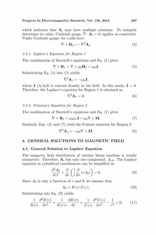
Progress In Electromagnetics Research, Vol. 136, 2013 287
which indicates that Ai may have multiple solutions. To uniquelydetermine its value, Coulomb gauge, ∇ ·Ai = 0, applies as constraint.Under Coulomb gauge, we could have
∇×Bi = −∇2Ai. (4)
3.2.1. Laplace’s Equation for Region 1
The combination of Maxwell’s equations and Eq. (1) gives
∇×B1 = ∇× µ0H1 = µ0J. (5)
Substituting Eq. (4) into (5) yields
∇2A1 = −µ0J,
where J (A/m2) is current density in the field. In this study, J = 0.Therefore, the Laplace’s equation for Region 1 is obtained as
∇2A1 = 0. (6)
3.2.2. Poission’s Equation for Region 2
The combination of Maxwell’s equations and Eq. (1) gives
∇×B2 = µ0µrJ + µ0∇×M. (7)
Similarly, Eqs. (4) and (7) yield the Poisson equation for Region 2
∇2A2 = −µ0∇×M. (8)
4. GENERAL SOLUTIONS TO MAGNETIC FIELD
4.1. General Solution to Laplace Equation
The magnetic field distribution of tubular linear machine is axiallysymmetric. Therefore, Ai has only one component, Ai,θ. The Laplaceequation in cylindrical coordinators can be simplified as
∂2Aθ
∂z2+
∂
∂r
(1r
∂
∂r(rAθ)
)= 0. (9)
Since Aθ is only a function of r and θ, we assume that
Aθ = R (r) Z (z) . (10)
Substituting into Eq. (9) yields
1R (r)
∂2R (r)∂r2
+1
R (r) r
∂R (r)∂r
+1
Z (z)∂2Z (z)
∂z2− 1
r2= 0, (11)

288 Yan et al.
where r and z are independent variables, and the third term asa function of z must be a constant. So the following formula isestablished
1Z (z)
∂2Z (z)∂z2
= k2. (12)
Then Eq. (11) becomes
1R (r)
∂2R (r)∂r2
+1
R (r) r
∂R (r)∂r
+ k2 − 1r2
= 0. (13)
Eq. (12) can then be rewritten as
∂2Z (z)∂z2
− k2Z (z) = 0. (14)
Thus, Laplace equation, Eq. (9), is separated into two equations,Eqs. (13) and (14). There are three possible solutions to Eqs. (13)and (14) according to variation of k.
4.1.1. The First Solution
When k2 = 0, the following equations are obtained
Z (z) = E0 + F0z, r2 ∂2R(r)∂r2 + r ∂R(r)
∂r −R (r) = 0. (15)
The solution to Eq. (15) is
Aθ = R (r) Z (z) =(
C0r + D01r
)(E0 + F0z) . (16)
However, as Aθ should be a periodic function of z, Eq. (16) is not thevalid solution of Aθ.
4.1.2. The Second Solution
When k2 > 0, the following equation is obtained
Z (z) = E0ekz + F0e
−kz,
r2 ∂2R (r)∂r2
+ r∂R (r)
∂r+ R (r)
(k2r2 − 1
)= 0.
(17)
The solution to Eq. (15) is
Aθ = R (r) Z (z) = [C0J1 (kr) + D0Y1 (kr)](E0e
kz + F0e−kz
). (18)
Again, because Eq. (18) is not a periodic function of z, it is not thesolution of Laplace’s equation either.
Progress In Electromagnetics Research, Vol. 136, 2013 289
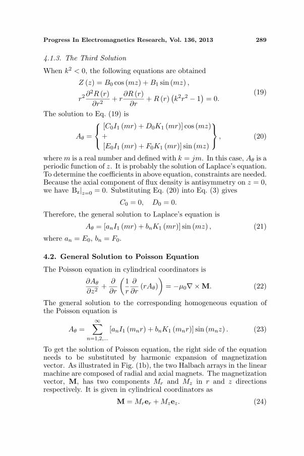
4.1.3. The Third Solution
When k2 < 0, the following equations are obtained
Z (z) = B0 cos (mz) + B1 sin (mz) ,
r2 ∂2R (r)∂r2
+ r∂R (r)
∂r+ R (r)
(k2r2 − 1
)= 0.
(19)
The solution to Eq. (19) is
Aθ =
[C0I1 (mr) + D0K1 (mr)] cos (mz)+[E0I1 (mr) + F0K1 (mr)] sin (mz)
, (20)
where m is a real number and defined with k = jm. In this case, Aθ is aperiodic function of z. It is probably the solution of Laplace’s equation.To determine the coefficients in above equation, constraints are needed.Because the axial component of flux density is antisymmetry on z = 0,we have Bz|z=0 = 0. Substituting Eq. (20) into Eq. (3) gives
C0 = 0, D0 = 0.
Therefore, the general solution to Laplace’s equation is
Aθ = [anI1 (mr) + bnK1 (mr)] sin (mz) , (21)
where an = E0, bn = F0.
4.2. General Solution to Poisson Equation
The Poisson equation in cylindrical coordinators is
∂Aθ
∂z2+
∂
∂r
(1r
∂
∂r(rAθ)
)= −µ0∇×M. (22)
The general solution to the corresponding homogeneous equation ofthe Poisson equation is
Aθ =∞∑
n=1,2,...
[anI1 (mnr) + bnK1 (mnr)] sin (mnz) . (23)
To get the solution of Poisson equation, the right side of the equationneeds to be substituted by harmonic expansion of magnetizationvector. As illustrated in Fig. (1b), the two Halbach arrays in the linearmachine are composed of radial and axial magnets. The magnetizationvector, M, has two components Mr and Mz in r and z directionsrespectively. It is given in cylindrical coordinators as
M = Mrer + Mzez. (24)
290 Yan et al.
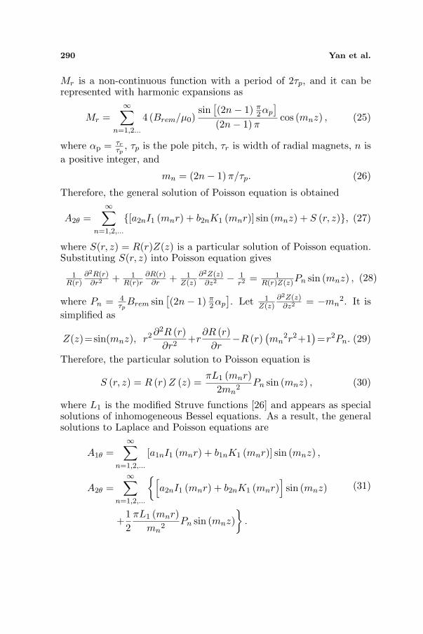
Mr is a non-continuous function with a period of 2τp, and it can berepresented with harmonic expansions as
Mr =∞∑
n=1,2...
4 (Brem/µ0)sin
[(2n− 1) π
2 αp
]
(2n− 1)πcos (mnz) , (25)
where αp = τrτp
, τp is the pole pitch, τr is width of radial magnets, n isa positive integer, and
mn = (2n− 1)π/τp. (26)
Therefore, the general solution of Poisson equation is obtained
A2θ =∞∑
n=1,2,...
{[a2nI1 (mnr) + b2nK1 (mnr)] sin (mnz) + S (r, z)}, (27)
where S(r, z) = R(r)Z(z) is a particular solution of Poisson equation.Substituting S(r, z) into Poisson equation gives
1R(r)
∂2R(r)∂r2 + 1
R(r)r∂R(r)
∂r + 1Z(z)
∂2Z(z)∂z2 − 1
r2 = 1R(r)Z(z)Pn sin (mnz) , (28)
where Pn = 4τp
Brem sin[(2n− 1) π
2 αp
]. Let 1
Z(z)∂2Z(z)
∂z2 = −mn2. It is
simplified as
Z(z)=sin(mnz), r2 ∂2R (r)∂r2
+r∂R (r)
∂r−R (r)
(mn
2r2+1)=r2Pn. (29)
Therefore, the particular solution to Poisson equation is
S (r, z) = R (r) Z (z) =πL1 (mnr)
2mn2
Pn sin (mnz) , (30)
where L1 is the modified Struve functions [26] and appears as specialsolutions of inhomogeneous Bessel equations. As a result, the generalsolutions to Laplace and Poisson equations are
A1θ =∞∑
n=1,2,...
[a1nI1 (mnr) + b1nK1 (mnr)] sin (mnz) ,
A2θ =∞∑
n=1,2,...
{[a2nI1 (mnr) + b2nK1 (mnr)
]sin (mnz)
+12
πL1 (mnr)mn
2Pn sin (mnz)
}.
(31)
Progress In Electromagnetics Research, Vol. 136, 2013 291
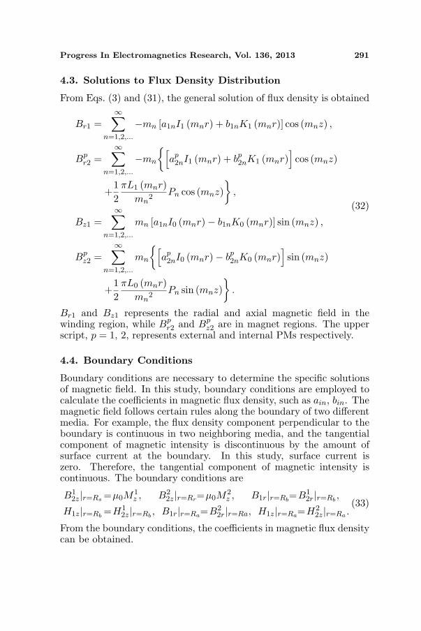
4.3. Solutions to Flux Density Distribution
From Eqs. (3) and (31), the general solution of flux density is obtained
Br1 =∞∑
n=1,2,...
−mn [a1nI1 (mnr) + b1nK1 (mnr)] cos (mnz) ,
Bpr2 =
∞∑
n=1,2,...
−mn
{[ap
2nI1 (mnr) + bp2nK1 (mnr)
]cos (mnz)
+12
πL1 (mnr)mn
2Pn cos (mnz)
},
Bz1 =∞∑
n=1,2,...
mn [a1nI0 (mnr)− b1nK0 (mnr)] sin (mnz) ,
Bpz2 =
∞∑
n=1,2,...
mn
{[ap
2nI0 (mnr)− bp2nK0 (mnr)
]sin (mnz)
+12
πL0 (mnr)mn
2Pn sin (mnz)
}.
(32)
Br1 and Bz1 represents the radial and axial magnetic field in thewinding region, while Bp
r2 and Bpz2 are in magnet regions. The upper
script, p = 1, 2, represents external and internal PMs respectively.
4.4. Boundary Conditions
Boundary conditions are necessary to determine the specific solutionsof magnetic field. In this study, boundary conditions are employed tocalculate the coefficients in magnetic flux density, such as ain, bin. Themagnetic field follows certain rules along the boundary of two differentmedia. For example, the flux density component perpendicular to theboundary is continuous in two neighboring media, and the tangentialcomponent of magnetic intensity is discontinuous by the amount ofsurface current at the boundary. In this study, surface current iszero. Therefore, the tangential component of magnetic intensity iscontinuous. The boundary conditions are
B12z|r=Rs =µ0M
1z , B2
2z|r=Rr=µ0M2z , B1r|r=Rb
=B12r|r=Rb
,
H1z|r=Rb=H1
2z|r=Rb, B1r|r=Ra=B2
2r|r=Ra, H1z|r=Ra=H22z|r=Ra .
(33)
From the boundary conditions, the coefficients in magnetic flux densitycan be obtained.
292 Yan et al.
5. NUMERICAL SIMULATION AND EXPERIMENTS
In this section, a research prototype of the linear machine with dualHalbach array and an experimental apparatus have been developed.The experimental works are conducted on the flux field distribution tovalidate the derived analytical models. Furthermore, the mathematicalfield model is compared with numerical results from FEM. AlthoughFEM is time-consuming, its precision is relatively high withoutsignificant influence from manufacturing and model simplification.Therefore, it is used to validate the magnetic analytical model andobserve the flux variation in machine space. The design parametersand material characteristics used in the numerical computation areconsistent with those in experiments. The finite element solutions areobtained by applying a master-slave boundary at the axial boundariesz = 0, z = τp and imposing symmetry boundary at z = 0. The highestorder of harmonics considered in the analytical solutions is 15.
5.1. Prototype and Experimental Apparatus
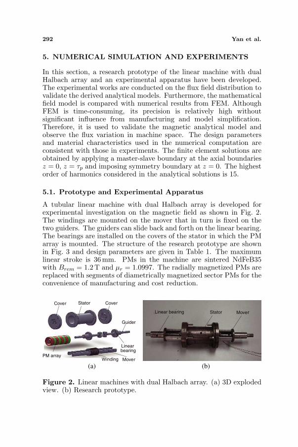
A tubular linear machine with dual Halbach array is developed forexperimental investigation on the magnetic field as shown in Fig. 2.The windings are mounted on the mover that in turn is fixed on thetwo guiders. The guiders can slide back and forth on the linear bearing.The bearings are installed on the covers of the stator in which the PMarray is mounted. The structure of the research prototype are shownin Fig. 3 and design parameters are given in Table 1. The maximumlinear stroke is 36 mm. PMs in the machine are sintered NdFeB35with Brem = 1.2T and µr = 1.0997. The radially magnetized PMs arereplaced with segments of diametrically magnetized sector PMs for theconvenience of manufacturing and cost reduction.
Cover Stator Cover
Guider
Linearbearing
Winding Mover
Stator MoverLinear bearing
(a) (b)
PM array
Figure 2. Linear machines with dual Halbach array. (a) 3D explodedview. (b) Research prototype.

Progress In Electromagnetics Research, Vol. 136, 2013 293
Rr
RaRb
Rs
R o
r p
L
Z
g
g
o
i
τ τ
Figure 3. Structure of the research prototype.
Table 1. Design parameters of research prototype.
Maximumradius Ro
30mm Outer rad of ext PM Rs 17mm
Machinelength L
89mm Inner rad of ext PM Rb 14mm
Width ofradial PM τr
9mm Outer rad of int PM Ra 9mm
Pole pitchτp
18mm Inner rad of int PM Rr 5mm
Number ofpoles n
4 Number of winding turns 100
Outer airgap go
0.2mm Inner air gap gi 0.2mm
An experimental apparatus is developed for magnetic fieldmeasurement in 3D space as illustrated in Fig. 4. The researchprototype is mounted on a platform of the apparatus. A gauss probeis installed on the end-effect of a three-axis translational stage. Underthe PC controller, the probe can pinpoint to any position inside thelinear machine and measure the flux density. The measured data canbe either displayed on the Gauss meter or transferred to PC.
5.2. Validation of Analytical Model
In this section, the analytical model of the magnetic field in the linearmachine is validated. For winding region, the mathematical model ofthe flux distribution is compared with both FEM and experimentalresults. For magnet region, the model is compared with FEM results,as the probe cannot measure the flux field at this region. Thenumerical model is built in Ansoft environment, using 2D-FEM. Design

294 Yan et al.
Three-axistranslational stage
Gauss probe
Gauss/Tesla meter
Linear machine
Connected to PC
Connected to
Gauss/Tesla meter
Platform
Figure 4. Experimental testbed for magnetic field measurement.
-0.02 -0.01 0 0.01 0.02
-0.8
-0.6
-0.4
-0.2
0
0.2
0.4
0.6
0.8
z
Br
AnalyticalFEMExperimental
-0.02 -0.01 0 0.01 0.02-0.1
-0.08
-0.06
-0.04
-0.02
0
0.02
0.04
0.06
0.08
0.1
z
Bz
AnalyticalFEMExperimental
(a) (b)
Figure 5. Magnetic field variation versus z at r = 11.5 mm. (a) Br
variation. (b) Bz variation.
parameters are the same as those in research prototype, and thesimulation is implemented by applying master and slave boundary atz = 0 and z = τp, and symmetry boundary at z = 0.
5.2.1. Magnetic Field Variation in Winding Region
Magnetic field variations versus axial distance z are measured andsimulated. Results at r = 11.5mm, 12 mm, 12.5 mm are presentedin Figs. 5, 6, and 7, respectively. In this study, experiments areconducted neighboring to the center of linear machine (z = 0) to reducethe longitude fringe effect. Variation of radial flux component thatinteracts with current input to produce axial force output is in sinewaveform approximately, and harmonic contents of radial flux densityat distinctive radius are shown in Fig. 8. It is found that the analytical

Progress In Electromagnetics Research, Vol. 136, 2013 295
-0.02 -0.01 0 0.01 0.02
-0.8
-0.6
-0.4
-0.2
0
0.2
0.4
0.6
0.8
z
Br
AnalyticalFEMExperimental
-0.02 -0.01 0 0.01 0.02
-0.2
-0.15
-0.1
-0.05
0
0.05
0.1
0.15
0.2
z
Bz
AnalyticalFEMExperimental
(a) (b)
Figure 6. Magnetic field variation versus z at r = 12 mm. (a) Br
variation. (b) Bz variation.
-0.02 -0.01 0 0.01 0.02
-0.8
-0.6
-0.4
-0.2
0
0.2
0.4
0.6
0.8
z
Br
AnalyticalFEMExperimental
-0.02 -0.01 0 0.01 0.02-0.25
-0.2
-0.15
-0.1
-0.05
0
0.05
0.1
0.15
0.2
0.25
z
Bz
AnalyticalFEMExperimental
(a) (b)
Figure 7. Magnetic field variation versus z at r = 12.5 mm. (a) Br
variation. (b) Bz variation.
models fit with the finite element results and experimental resultsclosely. The difference is caused by manufacturing errors, assemblyerrors and replacement of diametrically magnetized segmental PMs.
5.2.2. Magnetic Field Variation in the Magnet Region
Figures 9 and 10 present magnetic field variation versus axial distancez at the center radius of internal and external Halbach array, i.e.,r = (Rr + Ra)/2 and r = (Rb + Rs)/2, respectively. Magnetic field ineither magnet region varies in line with the magnetization vector M.Therefore, the radial flux component is even-symmetric about z = 0,while the axial field is odd-symmetric. However, the radial flux densityin the internal magnet area is greater than that in the external magnet

296 Yan et al.
0
0.1
0.2
0.3
0.4
0.5
0.6
0.7
1 5 9 11 13 15
Harmanic Order
Br
r=11.5mm
r=12mm
r=12.5mm
3 7
Figure 8. Harmonic content of radial flux density.
-0.02 -0.01 0 0.01 0.02-1.5
-1
-0.5
0
0.5
1
1.5
z
Br
AnalyticalFEM
-0.02 -0.01 0 0.01 0.02-1.5
-1
-0.5
0
0.5
1
1.5
z
Bz
AnalyticalFEM
(a) (b)
Figure 9. Field variation at the center of internal magnet area.(a) Variation of Br. (b) Variation of Bz.
-0.02 -0.01 0 0.01 0.02-0.8
-0.6
-0.4
-0.2
0
0.2
0.4
0.6
0.8
z
Br
AnalyticalFEM
-0.02 -0.01 0 0.01 0.021.5
1
0.5
0
0.5
1
1.5
z
Bz
AnalyticalFEM
(a) (b)
Figure 10. Field variation at the external magnet area. (a) Variationof Br. (b) Variation of Bz.
area due to a decreasing section crossed by constant flux lines. Theanalytical results fit with the finite element results well. The differenceis mainly caused by the simplification of models and FEM meshing.
Progress In Electromagnetics Research, Vol. 136, 2013 297
6. CONCLUSION
A novel dual Halbach magnet array is proposed in this paper forthe development of tubular linear machines. It helps to improvethe radial flux, and reduce the axial flux. The 3D magnetic fielddistribution is formulated analytically based on Laplace’s and Poisson’sequations. Numerical computation of magnetic field is conductedwith FEM method. It shows that the analytical model fits withthe numerical result closely. A research prototype and an automaticapparatus are developed for experimental purpose. The experimentalresult validates the analytical magnetic field model well. The analyticalmodel in this paper can be used for design optimization and controlimplementation of tubular electromagnetic linear machines. Theproposed dual Halbach array can also be utilized for rotary machines.
ACKNOWLEDGMENT
The authors acknowledge the financial support from the NationalNatural Science Foundation of China under grant 51175012, 51235002,the Program for New Century Excellent Talents in University of Chinaunder grant NCET-12-0032, the Fundamental Research Funds forthe Central Universities, and Science and the Technology on AircraftControl Laboratory.
REFERENCES
1. Stumberger, G., M. T. Aydemir, D. Zarko, and T. A. Lipo,“Design of a linear bulk superconductor magnet synchronousmotor for electromagnetic aircraft launch systems,” IEEETransactions on Applied Superconductivity, Vol. 14, No. 1, 54–62,2004.
2. Kou, B. Q., X. Z. Huang, H. X. Wu, and L. Y. Li,“Thrust and thermal characteristics of electromagnetic launcherbased on permanent magnet linear synchronous motors,” IEEETransactions on Magnetics, Vol. 45, No. 1, 358–362, 2009.
3. Thornton, R., M. T. Thompson, B. M. Perreault, and J. R. Fang,“Linear motor powered transportation,” Proceedings of the IEEE,Vol. 97, No. 11, 1754–1757, 2009.
4. Yan L. G., “The linear motor powered transportation developmentand application in China,” Proceedings of the IEEE, Vol. 97,No. 11, 1872–1880, 2009.
5. Yamada, H., M. Yamaguchi, M. Karita, Y. Matsuura, and

298 Yan et al.
S. Fukunaga, “Acute animal experiment using a linear motor-driven total artificial heart,” IEEE Translation Journal onMagnetics in Japan, Vol. 9, No. 6, 90–97, 1994.
6. Yamada, H., M. Yamaguchi, K. Kobayashi, Y. Matsuura, andH. Takano, “Development and test of a linear motor-driventotal artificial heart,” IEEE Engineering in Medicine and BiologyMagazine, Vol. 14, No. 11, 84–90, 1995.
7. Mohammadpour, A., A. Gandhi, and L. Parsa, “Winding factorcalculation for analysis of back EMF waveform in air-corepermanent magnet linear synchronous motors,” IET ElectricPower Applications, Vol. 6, No. 5, 253–259, 2012.
8. Wang, J. B. and D. Howe, “Design optimization of radiallymagnetized, iron-cored, tubular permanent-magnet machines anddrive systems,” IEEE Transactions on Magnetics, Vol. 40, No. 5,3262–3277, 2004.
9. Mahmoudi, A., N. A. Rahim, and W. P. Hew, “Axial-fluxpermanent-magnet motor design for electric vehicle direct driveusing sizing equation and finite element analysis,” Progress InElectromagnetics Research, Vol. 122, 467–496, 2012.
10. Wang, J., G. W. Jewell, and D. Howe, “A general frameworkfor the analysis and design of tubular linear permanent magnetmachines,” IEEE Transactions on Magnetics, Vol. 35, No. 3, 1986–2000, 1999.
11. Fang, J. R., D. B. Montgomery, and L. Roderick, “A novel magpipe pipeline transportation system using linear motor drives,”Proceedings of the IEEE, Vol. 97, No. 11, 1848–1855, 2009.
12. Gurol, H., “General atomics linear motor applications: Movingtowards deployment,” Proceedings of the IEEE, Vol. 97, No. 11,1864–1871, 2009.
13. Torkaman, H. and E. Afjei, “Magnetostatic field analysisregarding the effcts of dynamic eccentricity in switched reluctancemotor,” Progress In Electromagnetics Research M, Vol. 8, 163–180,2009.
14. Torkaman, H. and E. Afjei, “Comparison of two types of duallayer generator in field assisted mode utilizing 3D-FEM andexperimental verification,” Progress In Electromagnetics ResearchB, Vol. 23, 293–309, 2010.
15. Torkaman, H. and E. Afjei, “Comparison of three novel typesof two-phase switched reluctance motors using finite elementmethod,” Progress In Electromagnetics Research, Vol. 125, 151–164, 2012.

Progress In Electromagnetics Research, Vol. 136, 2013 299
16. Jian, L. and K.-T. Chau, “Design and analysis of a magnetic-geared electronic-continuously variable transmission system usingfinite element method,” Progress In Electromagnetics Research,Vol. 107, 47–61, 2010.
17. Touati, S., R. Ibtiouen, O. Touhami, and A. Djerdir,“Experimental investigation and optimization of permanentmagnet motor based on coupling boundary element method withpermeances network,” Progress In Electromagnetics Research,Vol. 111, 71–90, 2011.
18. Lecointe, J. P., B. Cassoret, and J.-F. Brudny, “Distinction oftoothing and saturation effects on magnetic noise of inductionmotors,” Progress In Electromagnetics Research, Vol. 112, 125–137, 2011.
19. Zhao, W., M. Cheng, R. Cao, and J. Ji, “Experimental comparisonof remedial single-channel operations for redundant flux-switchingpermanent-magnet motor drive,” Progress In ElectromagneticsResearch, Vol. 123, 189–204, 2012.
20. Mahmoudi, A., S. Kahourzade, N. A. Rahim, and W. P. Hew, “Im-provement to performance of solid-rotor-ringed line-start axial-flux permanent-magnet motor,” Progress In Electromagnetics Re-search, Vol. 124, 383–404, 2012.
21. Musolino, A., R. Rizzo, and E. Tripodi, “Tubular linear inductionmachine as a fast actuator: Analysis and design criteria,” ProgressIn Electromagnetics Research, Vol. 132, 603–619, 2012.
22. Matyas, A. R., K. A. Biro, and D. Fodorean, “Multi-phasesynchronous motor solution for steering applications,” ProgressIn Electromagnetics Research, Vol. 131, 63–80, 2012.
23. Youn, H. K., S. J. Chang, K. Sol, D. C. Yon, and L. Ju,“Analysis of hybrid stepping motor using 3D equivalent magneticcircuit network method based on trapezoidal element,” Journal ofApplied Physics, Vol. 91, No. 10, 8311–8313, 2002.
24. Amrhein, M. and P. T. Krein, “Induction machine modelingapproach based on 3-D magnetic equivalent circuit framework,”IEEE Transactions on Energy Conversion, Vol. 25, No. 2, 339–347, 2010.
25. Liu, C. and K.-T. Chau, “Electromagnetic design and analysisof double-rotor flux-modulated permanent-magnet machines,”Progress In Electromagnetics Research, Vol. 131, 81–97, 2012.
26. The Wolfram functions site, 2012, http://functions.wolfram.com/Bessel-TypeFunctions/StruveL/introductions/Struves/01/.