magnetotelluric impedance tensor tools (mitt)

Magnetotelluric Impedance Tensor Tools (MITT)User Guide

September, 2018

Ivan Romero-Ruiz1 and Jaume Pous1

1 Departament de Dinàmica de la Terra i de l'Oceà, Universitat de Barcelona, Martí i Franquès, s/n,08028 Barcelona, Spain. ( ivanromerorui z @ gmail.com ; [email protected] )

Introduction

This manual is a first draft to guide the practitioner through MITT program. MITT program ismanly constituted by four blocks: 1- Magnetotelluric impedance tensor representation (Apparentresistivity and phase curves, Impedance tensor and Mohr diagrams); 2-Probability Density Functions ofdifferent indexes which account for the dimensionality; 3- Perturbed Method to determine the ‘PhaseSensitive strike angle’ for 2D; 4- Galvanic Distortion tools for obtaining the galvanic distortion (withthe exception of the gain) in a general 2D/3D case. Given that the distortion parameters cannot bedetermined, the method is based on a constrained stochastic heuristic method, which consists ofexploring randomly the full space of the distortion parameters. The constraints imposed assume the 2D(or 1D) tendency for the shortest periods of the regional impedance tensor. In this way a uniquesolution fulfilling the constraints is obtained. The method is based on Romero-Ruiz and Pous (2018a,b).

Requirements

MITT program is constituted by a set of programs to analyze the impedance tensor, accordingly an edi file is needed. MITT program has been written in Python 2.7 and the following modules are required:

PyQt: PyQt is one of the two most popular Python bindings for the Qt cross-platformGUI/XML/SQL C++ framework ( http://pyqt.sourceforge.net/ ). We used PyQt4.

Pygame: is a set of Python modules designed for writing games (http://pygame.org).

NumPy: is the fundamental package for scientific computing with Python\\(http://www.numpy.org/).

SciPy: is a Python-based ecosystem of open-source software for mathematics, science, andengineering (http://www.scipy.org/).

matplotlib: is a plotting library which produces publication quality figures in a variety ofhardcopy formats and interactive environments across platforms\\(http://matplotlib.org/).

The program has only been tested in Linux OS.

1

mailto:[email protected]

http://matplotlib.org/

http://www.scipy.org/

http://www.numpy.org/

http://pygame.org/

http://pyqt.sourceforge.net/





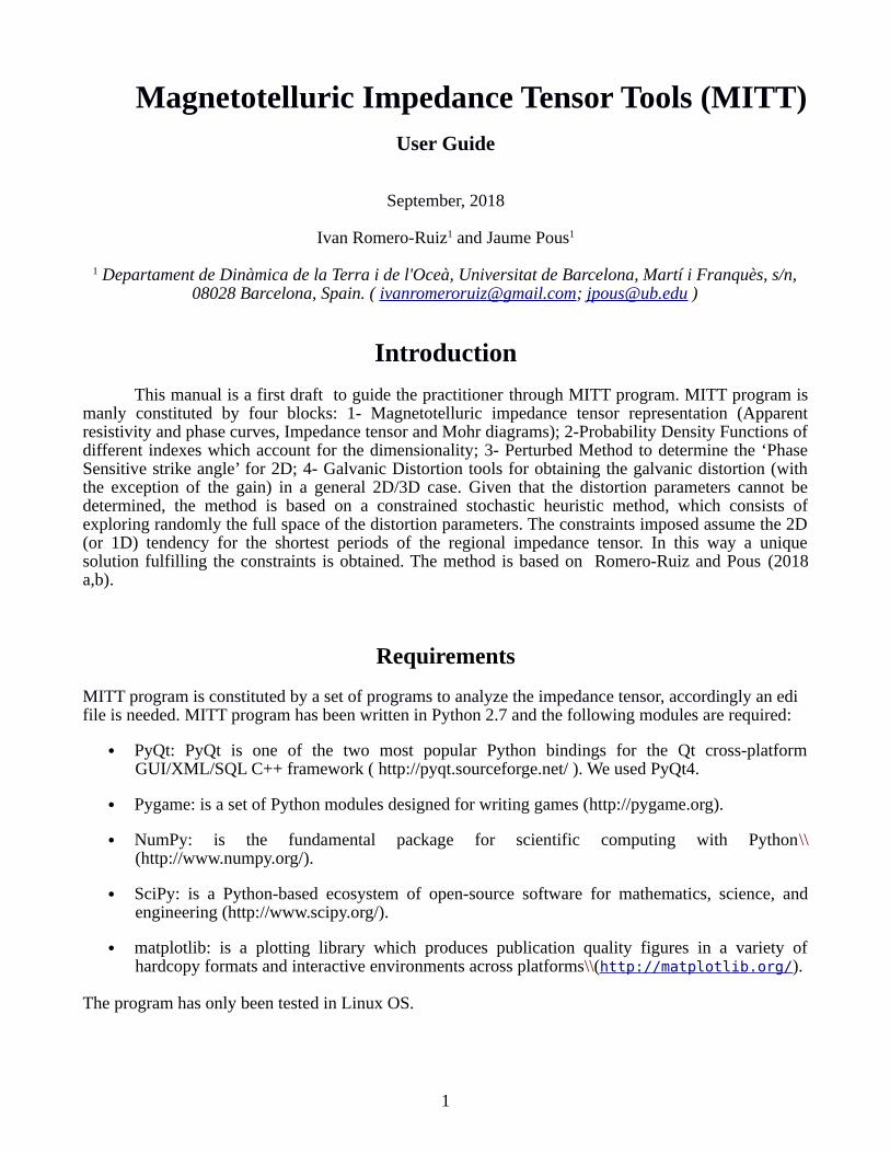
Block 1: Magnetotelluric Impedance tensor representation

MITT allows to draw different representations of the impedance tensor. After launched theprogram (python GUIDIS.pyc) select the Viewer menu and then the Viewer/Data/Curve Viewer sub-menu.

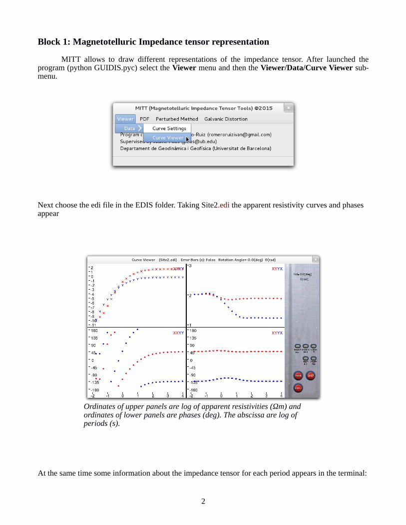
Next choose the edi file in the EDIS folder. Taking Site2.edi the apparent resistivity curves and phases appear

At the same time some information about the impedance tensor for each period appears in the terminal:

2

Ordinates of upper panels are log of apparent resistivities (Ωm) and ordinates of lower panels are phases (deg). The abscissa are log of periods (s).

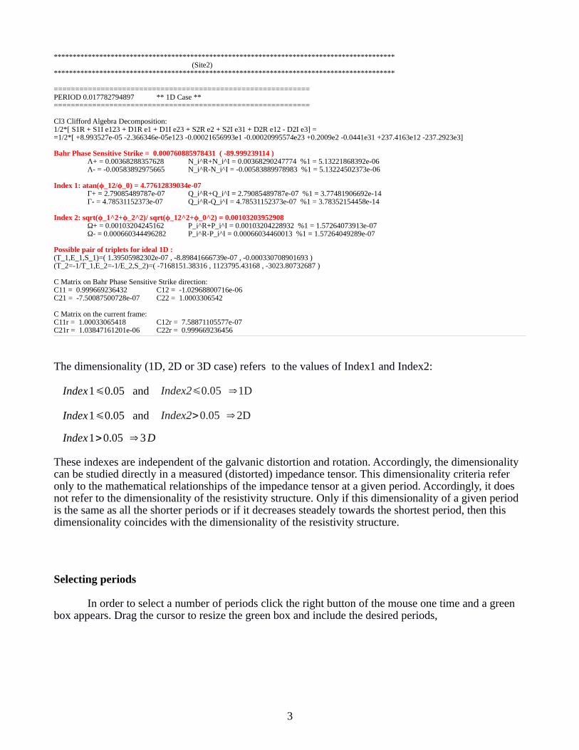
****************************************************************************************** (Site2) ******************************************************************************************

============================================================ PERIOD 0.017782794897 ** 1D Case ** ============================================================

Cl3 Clifford Algebra Decomposition: 1/2*[ S1R + S1I e123 + D1R e1 + D1I e23 + S2R e2 + S2I e31 + D2R e12 - D2I e3] = =1/2*[ +8.993527e-05 -2.366346e-05e123 -0.00021656993e1 -0.00020995574e23 +0.2009e2 -0.0441e31 +237.4163e12 -237.2923e3]

Bahr Phase Sensitive Strike = 0.000760885978431 ( -89.999239114 ) Λ+ = 0.00368288357628 N_i^R+N_iÎ = 0.00368290247774 %1 = 5.13221868392e-06 Λ- = -0.00583892975665 N_i^R-N_iÎ = -0.00583889978983 %1 = 5.13224502373e-06

Index 1: atan(ϕ_12/ϕ_0) = 4.77612839034e-07 Γ+ = 2.79085489787e-07 Q_i^R+Q_iÎ = 2.79085489787e-07 %1 = 3.77481906692e-14 Γ- = 4.78531152373e-07 Q_i^R-Q_iÎ = 4.78531152373e-07 %1 = 3.78352154458e-14

Index 2: sqrt(ϕ_1^2+ϕ_2^2)/ sqrt(ϕ_12^2+ϕ_0^2) = 0.00103203952908 Ω+ = 0.00103204245162 P_i^R+P_iÎ = 0.00103204228932 %1 = 1.57264073913e-07 Ω- = 0.000660344496282 P_i^R-P_iÎ = 0.00066034460013 %1 = 1.57264049289e-07

Possible pair of triplets for ideal 1D : (T_1,E_1,S_1)=( 1.39505982302e-07 , -8.89841666739e-07 , -0.000330708901693 ) (T_2=-1/T_1,E_2=-1/E_2,S_2)=( -7168151.38316 , 1123795.43168 , -3023.80732687 )

C Matrix on Bahr Phase Sensitive Strike direction: C11 = 0.999669236432 C12 = -1.02968800716e-06 C21 = -7.50087500728e-07 C22 = 1.0003306542

C Matrix on the current frame: C11r = 1.00033065418 C12r = 7.58871105577e-07 C21r = 1.03847161201e-06 C22r = 0.999669236456

The dimensionality (1D, 2D or 3D case) refers to the values of Index1 and Index2:

Index1⩽0.05 and Index2⩽0.05 ⇒1D

Index1⩽0.05 and Index2>0.05 ⇒2D

Index1>0.05 ⇒3 D

These indexes are independent of the galvanic distortion and rotation. Accordingly, the dimensionality can be studied directly in a measured (distorted) impedance tensor. This dimensionality criteria refer only to the mathematical relationships of the impedance tensor at a given period. Accordingly, it does not refer to the dimensionality of the resistivity structure. Only if this dimensionality of a given period is the same as all the shorter periods or if it decreases steadely towards the shortest period, then this dimensionality coincides with the dimensionality of the resistivity structure.

Selecting periods

In order to select a number of periods click the right button of the mouse one time and a green box appears. Drag the cursor to resize the green box and include the desired periods,

3

Then click one more time to select the periods included. The selection can be done in upper panels or lower panels.

By selecting periods, you specify which periods can be eliminated, depicted in Mohr diagrams or impedance tensor, as well as those periods in which the error bars can be recalculated and for which periods a Gaussian noise is added to the impedance tensor.

By selecting Viewer/Data/Curve Settings sub-menu, you may define the error bar recalculation (in %)and the Gaussian noise (in %) to be added to the impedance tensor.

4

The selected periods are shown in green.

The last four periods included in the green box will be selected.

Once a selection of periods has been made, press key “w” to assign error bar to the selected periods andthen key “q” (or button NOISE %) to add the Gaussian noise to the selected periods. ERROR BAR button shows the error bars. By clicking the button MENU, a list of the commands used by Curve Viewer sub-menu appears.

Curve Viewer sub-menu allows us to create a new edi file containing the current changes, such as noise, new error bars or rotation. The new edi file is created by clicking CREATE EDI button or pressing “o” key (an edi called filename_1.edi is created in /EDIS folder). When creating a new edi, all the selected periods are eliminated and the new picture is re-escaled. Accordingly, deselect previously the periods wanted in the new EDI file.

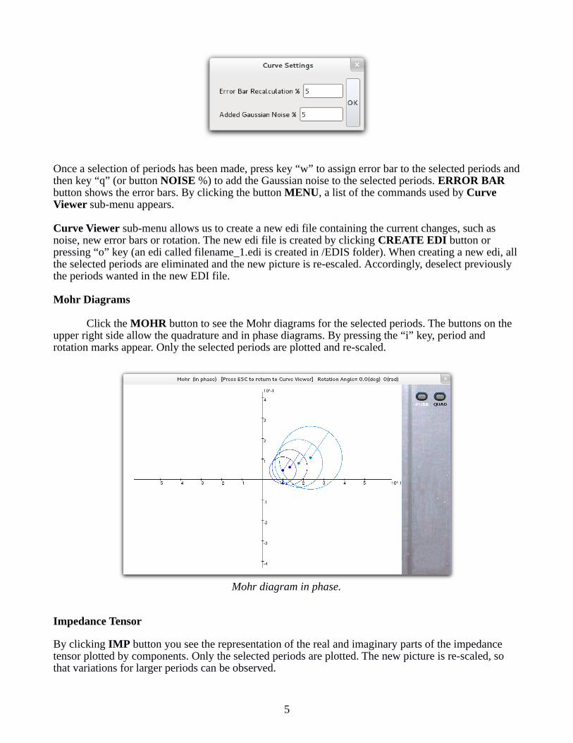
Mohr Diagrams

Click the MOHR button to see the Mohr diagrams for the selected periods. The buttons on the upper right side allow the quadrature and in phase diagrams. By pressing the “i” key, period and rotation marks appear. Only the selected periods are plotted and re-scaled.

Impedance Tensor

By clicking IMP button you see the representation of the real and imaginary parts of the impedance tensor plotted by components. Only the selected periods are plotted. The new picture is re-scaled, so that variations for larger periods can be observed.

5

Mohr diagram in phase.

General considerations

In all representations:

• rotation (spinning mouse wheel) and fine rotation (spinning mouse wheel + “f” key) can beinteractively seen.

• by pressing the “p” key a picture is taken, and automatically saved in the /pictures folder.

• press the “esc” key to return to the previous image.

The recalculation error bar and the Gauss noise addition are applied to the selectedperiods.

By creating an edi file, all selected periods are removed in the new edi file.

Block 2: Probability Density Function EstimationProbability Density Function (PDF) menu contains two sub-menus, Settings and Calculate.

By clicking the Calculate sub-menu, Bahr's Phase sensitive Strike, Index 1 and Index 2 PDF plots appear. The PDF depends on the values introduced in the Settings sub-menu.

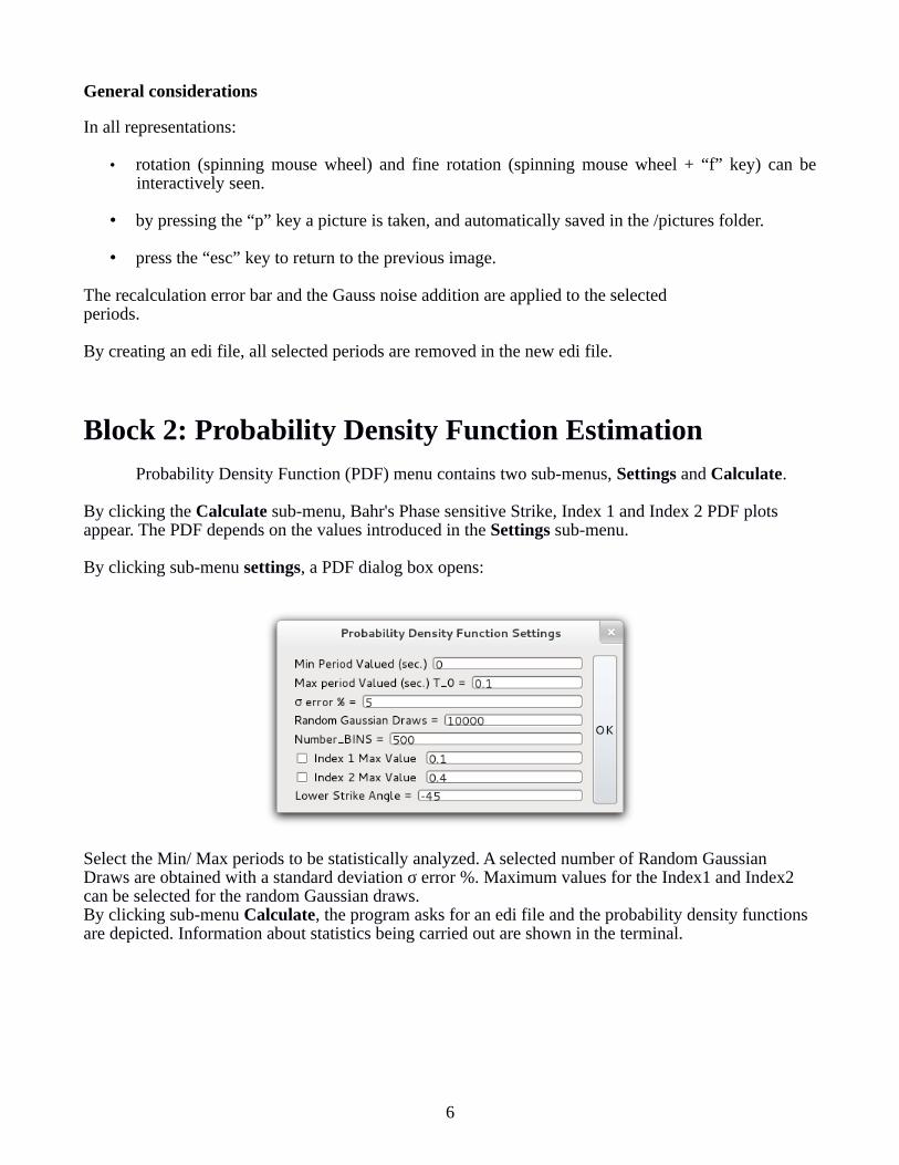
By clicking sub-menu settings, a PDF dialog box opens:

Select the Min/ Max periods to be statistically analyzed. A selected number of Random Gaussian Draws are obtained with a standard deviation σ error %. Maximum values for the Index1 and Index2 can be selected for the random Gaussian draws.By clicking sub-menu Calculate, the program asks for an edi file and the probability density functions are depicted. Information about statistics being carried out are shown in the terminal.

6

Block 3: Perturbed MethodIt provides, for the considered periods, an estimation of the Phase Sensitive Strike angle and a

Pseudoimpedance Tensor, which is the impedance tensor “corrected” of noise, so that all the selectedperiods have the same Phase Sensitive Strike angle. The perturbed method applies a Gaussianperturbation (like a noise correction) to the impedance tensor.

The Perturbed Method menu contains two sub-menus: Perturbed Method Settings and RegionalPhase Sensitive Strike.

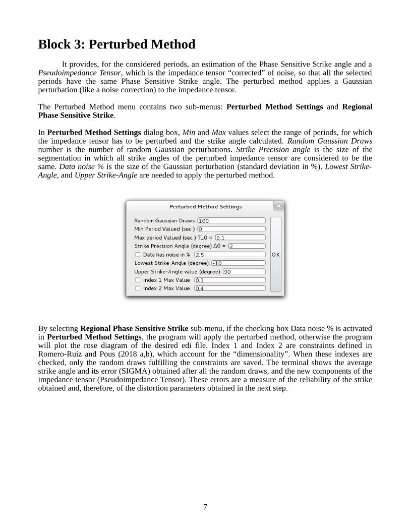
In Perturbed Method Settings dialog box, Min and Max values select the range of periods, for whichthe impedance tensor has to be perturbed and the strike angle calculated. Random Gaussian Drawsnumber is the number of random Gaussian perturbations. Strike Precision angle is the size of thesegmentation in which all strike angles of the perturbed impedance tensor are considered to be thesame. Data noise % is the size of the Gaussian perturbation (standard deviation in %). Lowest Strike-Angle, and Upper Strike-Angle are needed to apply the perturbed method.

By selecting Regional Phase Sensitive Strike sub-menu, if the checking box Data noise % is activatedin Perturbed Method Settings, the program will apply the perturbed method, otherwise the programwill plot the rose diagram of the desired edi file. Index 1 and Index 2 are constraints defined inRomero-Ruiz and Pous (2018 a,b), which account for the “dimensionality”. When these indexes arechecked, only the random draws fulfilling the constraints are saved. The terminal shows the averagestrike angle and its error (SIGMA) obtained after all the random draws, and the new components of theimpedance tensor (Pseudoimpedance Tensor). These errors are a measure of the reliability of the strikeobtained and, therefore, of the distortion parameters obtained in the next step.

7

Block 4: Galvanic DistortionThe Galvanic Distortion menu has two sub-menus: Add or Remove GD sub-menu, which

allows to add or remove a galvanic distortion, and Search sub-menu, which determines the galvanicdistortion parameters, twist (t), shear (e) and anisotropy (s). The best way to show how this tool worksis by showing an example. In the following section we are going to show the whole process step bystep.

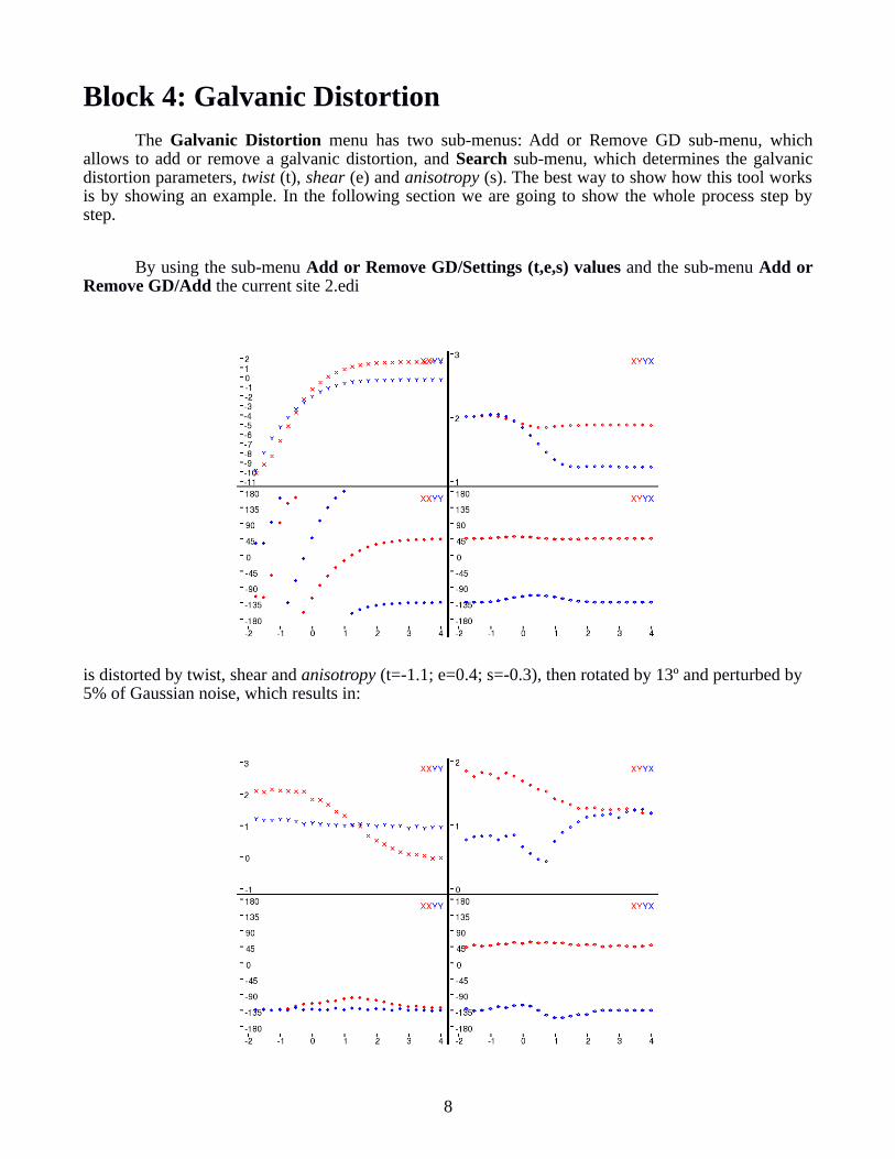
By using the sub-menu Add or Remove GD/Settings (t,e,s) values and the sub-menu Add orRemove GD/Add the current site 2.edi

is distorted by twist, shear and anisotropy (t=-1.1; e=0.4; s=-0.3), then rotated by 13º and perturbed by 5% of Gaussian noise, which results in:

8

Depicting this distorted, rotated and noisy site with Viewer/Data/Curve Viewer sub-menu, the terminal shows the following information for each period (only four periods shown here):

****************************************************************************************** (Site2(-1.1+0.4-0.3)_rot13_p5) ******************************************************************************************

============================================================ PERIOD 0.017782794897 ** 2D Case ** ============================================================

Cl3 Clifford Algebra Decomposition: 1/2*[ S1R + S1I e123 + D1R e1 + D1I e23 + S2R e2 + S2I e31 + D2R e12 - D2I e3] = =1/2*[ -176.519810293 -178.038890372e123 -84.6111723612e1 -82.5781968278e23 +75.0233207239e2+64.624144899e31 +128.533798716e12 -123.732549489e3]

Bahr Phase Sensitive Strike = 37.4188681018 ( -52.5811318982 ) Λ+ = 5.4533621445 N_i^R+N_iÎ = -2.40562094529 %1 = 1.44112620463 Λ- = 0.0614570345849 N_i^R-N_iÎ = 0.150024377584 %1 = 0.590353010794

Index 1: atan(ϕ_12/ϕ_0) = 0.00888539237385

Γ+ = 2.88111833885 Q_i^R+Q_iÎ = -2.81223481011 %1 = 1.97609139208 Γ- = 0.0220313156849 Q_i^R-Q_iÎ = 0.065567208966 %1 = 0.663988813428

Index 2: sqrt(ϕ_1^2+ϕ_2^2)/ sqrt(ϕ_12^2+ϕ_0^2) = 0.052674016489 Ω+ = 1.33618145087 P_i^R+P_iÎ = 1.00151480147 %1 = 0.250464971795 Ω- = 0.0273775258291 P_i^R-P_iÎ = 0.0342346370637 %1 = 0.200297471296

Possible pair of triplets for ideal 1D : (T_1,E_1,S_1)=( 0.542163039391 , 3.3060819716 , -2.48100485856 ) (T_2=-1/T_1,E_2=-1/E_2,S_2)=( -1.84446361582 , -0.302472839025 , -0.403062491615 )

C Matrix on Bahr Phase Sensitive Strike direction: C11 = 0.111666579638 C12 = 0.915446070736 C21 = -0.542278059215 C22 = 0.924891114164

C Matrix on the current frame: C11r = 0.80471854955 C12r = 1.07251803225 C21r = -0.385206097704 C22r = 0.231839144253

============================================================ PERIOD 0.0316227732034 ** 2D Case ** ============================================================


Bahr Phase Sensitive Strike = -64.5994994736 ( 25.4005005264 ) Λ+ = 3.1311755513 N_i^R+N_iÎ = -2.75726063515 %1 = 1.88058321546 Λ- = -0.0982834535858 N_i^R-N_iÎ = -0.283113666757 %1 = 0.652848077906

Index 1: atan(ϕ_12/ϕ_0) = 0.0131196123365 Γ+ = 2.79292473424 Q_i^R+Q_iÎ = -2.84076624416 %1 = 1.98315894171 Γ- = -0.0125541406025 Q_i^R-Q_iÎ = -0.037877468434 %1 = 0.668559142901

Index 2: sqrt(ϕ_1^2+ϕ_2^2)/ sqrt(ϕ_12^2+ϕ_0^2) = 0.0630501642085 Ω+ = 1.25285621407 P_i^R+P_iÎ = 0.962750340727 %1 = 0.231555600781 Ω- = -0.0209518757262 P_i^R-P_iÎ = -0.0258033998975 %1 = 0.188018795606

Possible pair of triplets for ideal 1D : (T_1,E_1,S_1)=( 0.572194734293 , -2.32030814397 , 4.65568817446 ) (T_2=-1/T_1,E_2=-1/E_2,S_2)=( -1.747656768 , 0.430977240071 , 0.214791017467 )



9

============================================================ PERIOD 0.0562341454856 ** 1D Case ** ============================================================


Bahr Phase Sensitive Strike = -70.0865615298 ( 19.9134384702 ) Λ+ = 2.69494778894 N_i^R+N_iÎ = -2.88253898824 %1 = 1.93492153963 Λ- = -0.0569845796942 N_i^R-N_iÎ = -0.174920348636 %1 = 0.674225553868






============================================================ PERIOD 0.1 ** 1D Case ** ============================================================


Bahr Phase Sensitive Strike = 3.83674538185 ( -86.1632546181 ) Λ+ = 3.10796409538 N_i^R+N_iÎ = -2.74661575353 %1 = 1.88373471161 Λ- = 0.0328231720242 N_i^R-N_iÎ = 0.0946533205114 %1 = 0.653227463687



Possible pair of triplets for ideal 1D : (T_1,E_1,S_1)=( 0.750277267686 , 2.0656874802 , 12.4671012266 ) (T_2=-1/T_1,E_2=-1/E_2,S_2)=( -1.33284059516 , -0.484100334434 , 0.0802111077647 )

C Matrix on Bahr Phase Sensitive Strike direction: C11 = -0.206347359917 C12 = -0.4203437684 C21 = 1.05679584249 C22 = -0.814809444417

C Matrix on the current frame: C11r = -0.769593100351 C12r = -1.09456941759 C21r = 0.382570193302 C22r = -0.251563703982

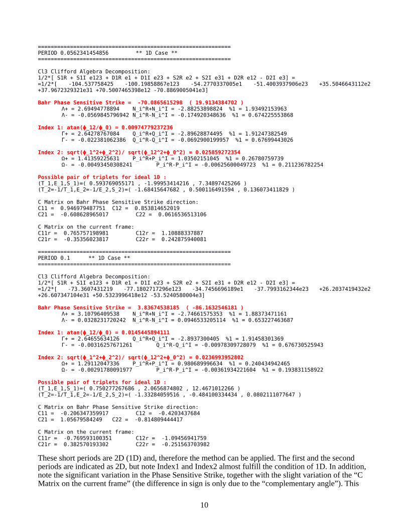
These short periods are 2D (1D) and, therefore the method can be applied. The first and the second periods are indicated as 2D, but note Index1 and Index2 almost fulfill the condition of 1D. In addition, note the significant variation in the Phase Sensitive Strike, together with the slight variation of the “C Matrix on the current frame” (the difference in sign is only due to the “complementary angle”). This

10

happens typically in 1D cases. In order to show how the program works in a 2D case, higher periodsbetween 0.3s and 2s, which are really 2D, will be considered later, allowing to compare the results.

Perturbed Method

Leaving non-checked the “Data has noise %” checkbox in Perturbation Method Settings, the rose diagram for these periods is depicted with a 1º segment precision. That is

Next, we start the Perturbed method with the following settings. Note the “Data has noise %” checkboxis checked.

11

Rose Diagram for the Site 2 distorted, rotated, and with noise. Each period has different Phase Sensitive strike angle due to noise.

The results are shown in terminal. The Phase Sensitive Strike angle obtained is 27.67º±2.9º and a new file in the EDIS folder appear (Site2(-1.1+0.4-0.3)_rot13_p5_ZP-1.0p_A5.0_I1-0.1.edi). It is labeled with _ZP to denote the pseudo impedance tensor corrected from noise.

Plotting the rose diagram of this edi file (Data has noise % not checked):

Note the Pseudoimpedance Tensor gives a unique Phase Sensitive strike within the Strike PrecisionAngle (Δθ). To continue the process the edi file should be rotated to the Phase Sensitive strike angle.However, in 1D case to continue with the process to find the galvanic distortion parameters any anglecan be used due to the independence of the regional impedance tensor with rotation (1D case). Thegalvanic distortion parameters obtained at different angles are connected by rotations. Therefore, all thegalvanic distortion parameters coincide when derotating by the corresponding angle.

12

Galvanic Distortion Correction

In this example, only one period is considered to correct the galvanic distortion. Accordingly, we chose the lowest period 0.0178s. First, we rotate to the Phase Sensitive strike specific for 0.0178s, which is -61.36o (shown in the terminal when depicting the site with Curve Viewer). In case of choosing more periods, the Phase Sensitive Strike angle obtained in the Perturbed Method should be chosen. By plotting the rotated site, the following information appears in the terminal:

****************************************************************************************** (Site2(-1.1+0.4-0.3)_rot13_p5_ZP-1.0p_A5.0_I1-0.1_rot-61,36) ******************************************************************************************

============================================================ PERIOD 0.017782794897 ** 2D Case ** ============================================================

Cl3 Clifford Algebra Decomposition: 1/2*[ S1R + S1I e123 + D1R e1 + D1I e23 + S2R e2 + S2I e31 + D2R e12 - D2I e3] = =1/2*[ -175.897395184 -178.869923131e123 -18.3335267286e1 -8.7913655836e23 -110.479295888e2 -105.864788848e31+128.673850168e12 -123.86449744e3]

Bahr Phase Sensitive Strike = -89.9931650765 ( 0.00683492354294 ) Λ+ = 0.252467874318 N_i^R+N_iÎ = 0.248988701141 %1 = 0.0137806569913 Λ- = 0.0817751077668 N_i^R-N_iÎ = 0.0829020224774 %1 = 0.0135933319463

Index 1: atan(ϕ_12/ϕ_0) = 0.00728181494971 Γ+ = 2.88595084285 Q_i^R+Q_iÎ = -2.81107929461 %1 = 1.9740565407 Γ- = 0.0259159609247 Q_i^R-Q_iÎ = 0.0770755330966 %1 = 0.66375891436





============================================================ PERIOD 0.0316227732034 ** 2D Case ** ============================================================


Bahr Phase Sensitive Strike = -1.29152587775 ( 88.7084741223 ) Λ+ = 0.120220963134 N_i^R+N_iÎ = 0.120046741878 %1 = 0.0014491753483 Λ- = -0.0926801225469 N_i^R-N_iÎ = -0.0928144322958 %1 = 0.00144707827813



Possible pair of triplets for ideal 1D :

13

(T_1,E_1,S_1)=( 0.562145568671 , -2.3963064463 , 4.15921801396 ) (T_2=-1/T_1,E_2=-1/E_2,S_2)=( -1.77889866207 , 0.417308897009 , 0.240429810759 )



============================================================ PERIOD 0.0562341454856 ** 1D Case ** ============================================================


Bahr Phase Sensitive Strike = -1.24182958898 ( 88.758170411 ) Λ+ = 0.0730953250689 N_i^R+N_iÎ = 0.0730464384293 %1 = 0.000668806652054 Λ- = -0.0515460990911 N_i^R-N_iÎ = -0.051580573465 %1 = 0.000668359648675






============================================================ PERIOD 0.1 ** 1D Case ** ============================================================


Bahr Phase Sensitive Strike = 88.4738100096 ( -1.52618999041 ) Λ+ = 0.11821489119 N_i^R+N_iÎ = 0.11781253591 %1 = 0.00340359218493 Λ- = 0.0162366026122 N_i^R-N_iÎ = 0.016291865386 %1 = 0.00339204704014




C Matrix on Bahr Phase Sensitive Strike direction: C11 = 0.0706441964795 C12 = 0.740706576654

14

C21 = -0.736019228107 C22 = 0.95112504996


Note that after this rotation, the Phase Sensitive Strike, for the considered periods, must be approximately zero.

The program allows to use different constraints which the regional impedance tensor (free of galvanic distortion) should fulfill for the short periods, between T_min and T_max:

• Off-diagonal components of the regional impedance tensor fulfill Zxy >0 and Zyx < 0 .• The diagonal apparent resistivities should be lower than the specified value.• Values for t and e may be specified from the terminal information above, which makes the

search faster. From the two possible triplets (t,e,s) for the ideal 1D case, appearing in the terminal, it is recommended to select that with the lower anisotropy s parameter absolute value (specified in green above).

• Indexes γ, λ and ε are expected to be lower than the specified values.

These indexes are defined in Romero-Ruiz and Pous (2018 a,b).

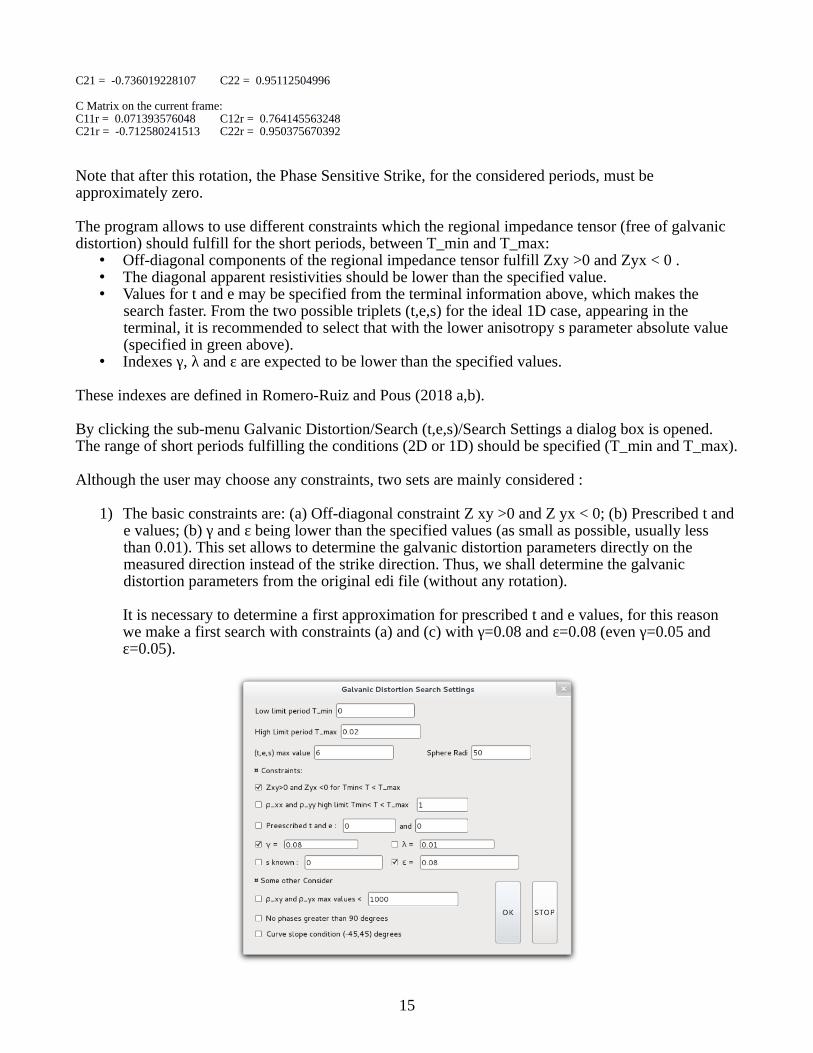
By clicking the sub-menu Galvanic Distortion/Search (t,e,s)/Search Settings a dialog box is opened. The range of short periods fulfilling the conditions (2D or 1D) should be specified (T_min and T_max).

Although the user may choose any constraints, two sets are mainly considered :

1) The basic constraints are: (a) Off-diagonal constraint Z xy >0 and Z yx < 0; (b) Prescribed t and e values; (b) γ and ε being lower than the specified values (as small as possible, usually less than 0.01). This set allows to determine the galvanic distortion parameters directly on the measured direction instead of the strike direction. Thus, we shall determine the galvanic distortion parameters from the original edi file (without any rotation).

It is necessary to determine a first approximation for prescribed t and e values, for this reason we make a first search with constraints (a) and (c) with γ=0.08 and ε=0.08 (even γ=0.05 and ε=0.05).

15

Once a prescribed values for t and e are obtained, we may apply all the constraints of the first set.

2) The basic constraints are: (a) Off-diagonal constraint Z xy >0 and Z yx < 0; (b) Prescribed t and e values; (c) diagonal apparent resistivities that should be lower than the prescribed value; (d) ε being lower than the specified value (as small as possible).

Once entering the selected inputs, click OK and then click sub-menu Galvanic Distortion/Search (t,e,s)/Search, to start the search.

By using the first set of constraints above, once the process ends, click Galvanic Distortion/Search/Plotting Results sub-menu and select Site2(-1.1+0.4-0.3)_rot13,006_p5.edi (instead Site2(-1.1+0.4-0.3)_rot13,006_p5_ZP-1.0p_A5.0_I1-0.1_rot-61,36.edi) file to obtain the figure:

16

In the terminal, the obtained distortion parameter values appear:

_________ ___/SOLUTIONS \______________________(t,e,s) = ( -1.270379 , 0.4844691 , -0.1071289 )(θt,θe,θs) = ( -51.7913575 , 25.848755 , -6.1147128 ) +-( 0.4367361 , 0.634059 , 0.8999332 )

In order to correct the galvanic distortion and obtain the regional impedance tensor, click the sub-menuGalvanic Distortion/Add or Remove GD/Settings (t,e,s) values

then click Galvanic Distortion/Add or Remove GD/Remove to create an edi file corrected of galvanicdistortion. This edi file correspond to axes rotated (13o). In order to compare with the original syntheticSite2 (not rotated), the current edi must be rotated to -13o resulting:

17

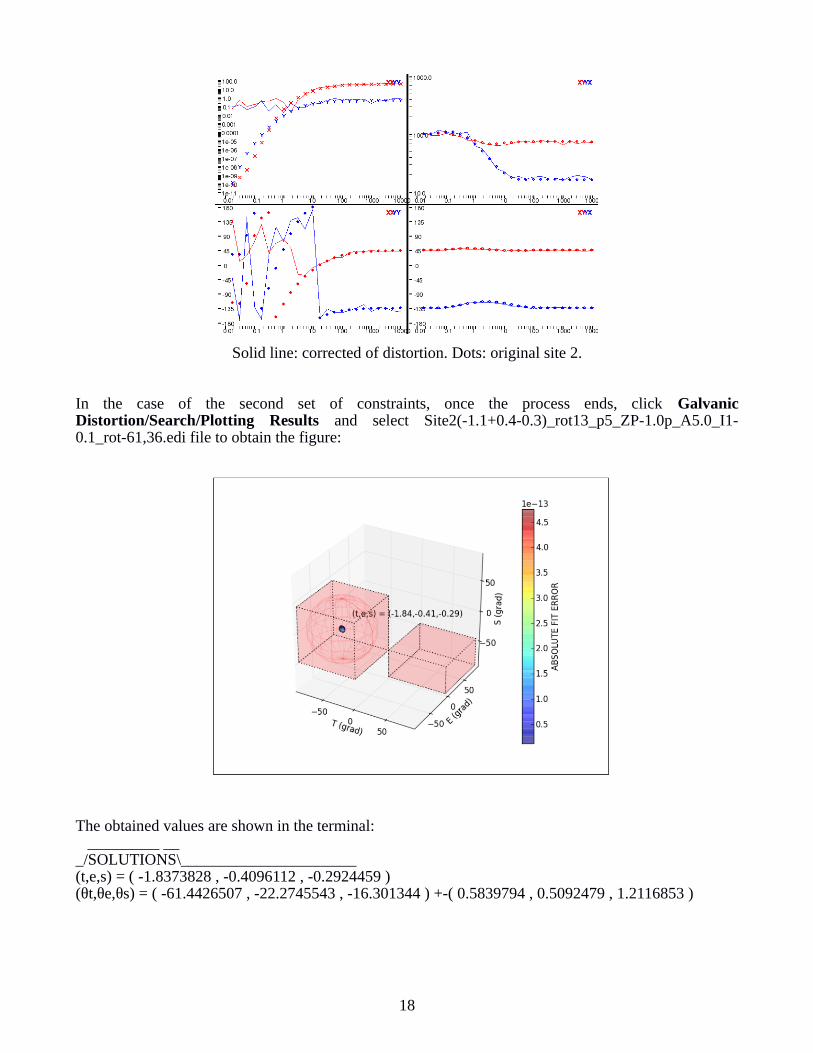
Solid line: corrected of distortion. Dots: original site 2.

In the case of the second set of constraints, once the process ends, click GalvanicDistortion/Search/Plotting Results and select Site2(-1.1+0.4-0.3)_rot13_p5_ZP-1.0p_A5.0_I1-0.1_rot-61,36.edi file to obtain the figure:

The obtained values are shown in the terminal: _________ ___/SOLUTIONS\______________________(t,e,s) = ( -1.8373828 , -0.4096112 , -0.2924459 )(θt,θe,θs) = ( -61.4426507 , -22.2745543 , -16.301344 ) +-( 0.5839794 , 0.5092479 , 1.2116853 )

18

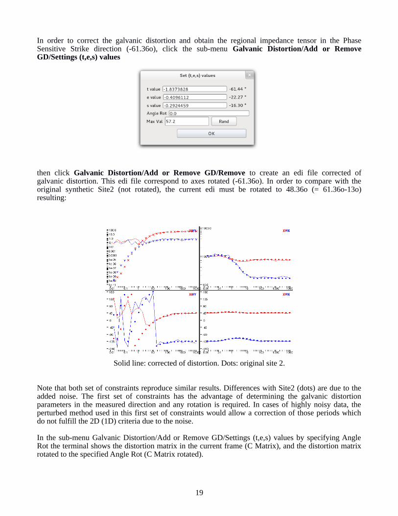
In order to correct the galvanic distortion and obtain the regional impedance tensor in the PhaseSensitive Strike direction (-61.36o), click the sub-menu Galvanic Distortion/Add or RemoveGD/Settings (t,e,s) values

then click Galvanic Distortion/Add or Remove GD/Remove to create an edi file corrected ofgalvanic distortion. This edi file correspond to axes rotated (-61.36o). In order to compare with theoriginal synthetic Site2 (not rotated), the current edi must be rotated to 48.36o (= 61.36o-13o)resulting:


Note that both set of constraints reproduce similar results. Differences with Site2 (dots) are due to theadded noise. The first set of constraints has the advantage of determining the galvanic distortionparameters in the measured direction and any rotation is required. In cases of highly noisy data, theperturbed method used in this first set of constraints would allow a correction of those periods whichdo not fulfill the 2D (1D) criteria due to the noise.

In the sub-menu Galvanic Distortion/Add or Remove GD/Settings (t,e,s) values by specifying AngleRot the terminal shows the distortion matrix in the current frame (C Matrix), and the distortion matrixrotated to the specified Angle Rot (C Matrix rotated).

19

Repetition with a new selection of the short periods

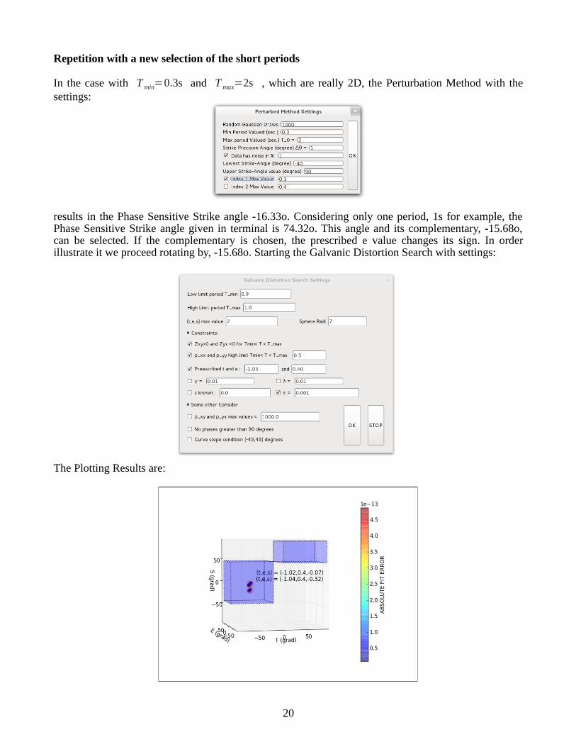
In the case with T min=0.3s and T max=2s , which are really 2D, the Perturbation Method with thesettings:

results in the Phase Sensitive Strike angle -16.33o. Considering only one period, 1s for example, thePhase Sensitive Strike angle given in terminal is 74.32o. This angle and its complementary, -15.68o,can be selected. If the complementary is chosen, the prescribed e value changes its sign. In orderillustrate it we proceed rotating by, -15.68o. Starting the Galvanic Distortion Search with settings:

The Plotting Results are:

20

And the terminal shows: ___________/SOLUTIONS\______________________(t,e,s) = ( -1.0159245 , 0.3985394 , -0.072834 )(θt,θe,θs) = ( -45.4525904 , 21.7292317 , -4.1657234 ) +-( 1.1801291 , 0.2082965 , 1.1074383 )(t,e,s) = ( -1.0434373 , 0.3965492 , -0.3161543 )(θt,θe,θs) = ( -46.2177518 , 21.6307627 , -17.5445762 ) +-( 0.9038443 , 0.5272168 , 0.7013945 )

The terminal gives two possible solutions because of the 2D case of this period (Romero-Ruiz and Pous2018 a,b). By plotting the corrected edis for both triplets, the right solution is identified:

For the triplet (t,e,s) = ( -1.0159245 , 0.3985394 , -0.072834 ) the regional impedance tensor rotated to2.68 (15.68o-13o) is:

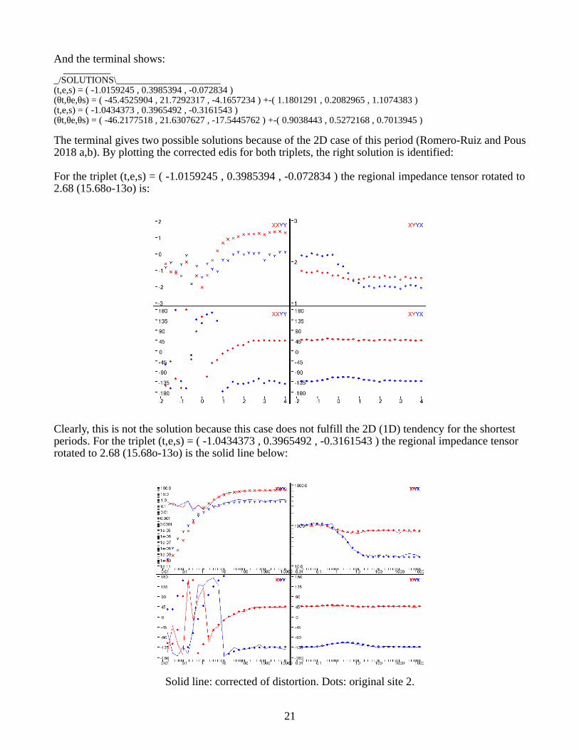
Clearly, this is not the solution because this case does not fulfill the 2D (1D) tendency for the shortest periods. For the triplet (t,e,s) = ( -1.0434373 , 0.3965492 , -0.3161543 ) the regional impedance tensor rotated to 2.68 (15.68o-13o) is the solid line below:


21

Dots are the original Site2 rotated to 13º. It is clear this last triplet is the correct solution.

REFERENCES

Romero-Ruiz, I. and Pous, J. (2018 a).The magnetotelluric impedance tensor through Clifford algebras:Part I — theory. Geophysical Prospecting, submitted.

Romero-Ruiz, I. and Pous, J. (2018 b).The magnetotelluric impedance tensor through Clifford algebras:Part II — a constrained stochastic heuristic method for recovering the magnetotelluric regional impedance tensor in 2D/3D case. Geophysical Prospecting, submitted.

22

magnetotelluric impedance tensor tools (mitt)

Documents