magnitude and frequency of floods on nontidal streams in delaware
TRANSCRIPT

Magnitude and Frequency of Floods on Nontidal Streams in Delaware
By Kernell G. Ries III and Jonathan J.A. Dillow
Prepared in cooperation with the Delaware Department of Transportation and the Delaware Geological Survey
Scientific Investigations Report 2006-5146
U.S. Department of the Interior U.S. Geological Survey

U.S. Department of the InteriorDIRK KEMPTHORNE, Secretary
U.S. Geological SurveyMark D. Myers, Director
U.S. Geological Survey, Reston, Virginia: 2006
For product and ordering information: World Wide Web: http://www.usgs.gov/pubprod Telephone: 1-888-ASK-USGS
For more information on the USGS--the Federal source for science about the Earth, its natural and living resources, natural hazards, and the environment: World Wide Web: http://www.usgs.gov Telephone: 1-888-ASK-USGS
Any use of trade, product, or firm names is for descriptive purposes only and does not imply endorsement by the U.S. Government.
Although this report is in the public domain, permission must be secured from the individual copyright owners to reproduce any copyrighted materials contained within this report.
Suggested citation:Ries, K.G., III, and Dillow, J.J.A., 2006, Magnitude and frequency of floods on nontidal streams in Delaware: U.S. Geological Survey Scientific Investigations Report 2006-5146, 59 p.

iii
Contents
Abstract ............................................................................................................................................................. 1Introduction....................................................................................................................................................... 1Physical Setting................................................................................................................................................ 2Methods for Estimating the Magnitude and Frequency of Floods .......................................................... 2
Flood-Frequency Analysis at Streamgaging Stations ...................................................................... 4Analysis of and Adjustments for Trends in Annual Peak-Flow Time Series ........................ 12Regional Skew Analysis ............................................................................................................... 15
Regional Flood-Frequency Relations ................................................................................................... 17Explanatory Variable Selection and Measurement ................................................................. 17Development of Regression Equations ...................................................................................... 22Accuracy and Limitations ............................................................................................................. 24Comparison of Results with Previous Study ............................................................................. 28
Application of the Methods ............................................................................................................................ 30Estimation for a Gaged Location .......................................................................................................... 30Estimation for a Site Upstream or Downstream from a Gaged Location ...................................... 31Estimation for a Site Between Gaged Locations ............................................................................... 32
Effects of Urbanization on Floods ................................................................................................................. 33StreamStats ...................................................................................................................................................... 35Summary and Conclusions ............................................................................................................................. 35References ........................................................................................................................................................ 36
Figures 1. Map showing study area and physiographic provinces in Delaware and
surrounding states ......................................................................................................................... 3 2. Map showing location of streamgaging stations in Delaware and surrounding
states for which flood-frequency estimates were computed ................................................. 5 3. Example flood-frequency curve produced by the PEAKFQ program for Beaverdam
Branch at Matthews, Maryland ................................................................................................... 11 4. Graph showing relation between 2000 housing density and 2001 impervious
surface percentage for streamgaging stations in and within 25 miles of Delaware .......... 13 5. Time-series plot showing adjustment of annual-peak flows for Stockley Branch
at Stockley, Delaware for an increasing trend with time......................................................... 13 6. Map showing skew ranges for streamgaging stations in Delaware and surrounding
states with 25 or more years of record ....................................................................................... 16 7. Graph showing relation between the new ArcHydro and the traditional 10/85 method
for measuring main channel slope for stations used in the regression analysis ................ 21 8. Boxplot showing percent storage measured using the National Hydrography
Dataset (NHD) and a combination of the 2001 National Land Cover Dataset (NLCD) and the 2002 Delaware Land-Use Dataset (DELU) .................................................................... 22

iv
Tables 1. Summary of streamgaging stations in and near Delaware for which
streamflow statistics were computed ......................................................................................... 6 2. Description of treatment of stations with annual peak-flow time series that were
affected by trends ........................................................................................................................... 14 3. Number of streamgaging stations included in the regression analyses by
hydrologic region and state .......................................................................................................... 18 4. Summary of drainage area, number of streamgaging stations, and average years
of record used in the regression analyses for Delaware ........................................................ 18 5. Basin characteristics considered for use in the regression analyses .................................. 19 6. Climatic characteristics for stations in and near Delaware that were considered
for use in the regression analyses ............................................................................................... 40 7. Basin characteristics for stations in and near Delaware that were considered
for use in the regression analyses ............................................................................................... 44 8. Flood-frequency statistics for stations in and near Delaware that were
considered for use in the regression analyses ......................................................................... 52 9. Average standard errors of estimate and prediction and equivalent years of record
for the best regression equations, by hydrologic region in Delaware .................................. 25 10. Values needed to determine 90-percent prediction intervals for the best regression
equations, by hydrologic region in Delaware ........................................................................... 26 11. Ranges of basin characteristics used to develop the regression equations ....................... 28 12. Mean and median percent differences between peak-flow frequency statistics
computed from the systematic records for streamgaging stations included in this study and the previous study ................................................................................................ 29
13. Matrix of correlations between the logarithms of flood-frequency estimates at the 2- and 100-year recurrence intervals and the logarithms of the indicators of urbanization ..................................................................................................................................... 34
14. Average standard errors of estimate and prediction and equivalent years of record for the urban regression equations ................................................................................ 34

v
Conversion Factors and Datum
Multiply By To obtain Length
foot (ft) 0.3048 meter (m)mile (mi) 1.609 kilometer (km)
Areasquare mile (mi2) 259.0 hectare (ha)square mile (mi2) 2.590 square kilometer (km2)
Flow ratecubic foot per second (ft3/s) 0.02832 cubic meter per second (m3/s)
Temperature in degrees Fahrenheit (°F) may be converted to degrees Celsius (°C) as follows:
°C=(°F-32)/1.8
Vertical coordinate information is referenced to North American Vertical Datum of 1988 (NAVD 88).
Horizontal coordinate information is referenced to North American Datum of 1983 (NAD 83).
Altitude, as used in this report, refers to distance above the vertical datum.


AbstractReliable estimates of the magnitude and frequency of
annual peak flows are required for the economical and safe design of transportation and water-conveyance structures. This report, done in cooperation with the Delaware Depart-ment of Transportation (DelDOT) and the Delaware Geologi-cal Survey (DGS), presents methods for estimating the magni-tude and frequency of floods on nontidal streams in Delaware at locations where streamgaging stations monitor streamflow continuously and at ungaged sites. Methods are presented for estimating the magnitude of floods for return frequencies rang-ing from 2 through 500 years. These methods are applicable to watersheds exhibiting a full range of urban development conditions. The report also describes StreamStats, a web application that makes it easy to obtain flood-frequency esti-mates for user-selected locations on Delaware streams.
Flood-frequency estimates for ungaged sites are obtained through a process known as regionalization, using statistical regression analysis, where information determined for a group of streamgaging stations within a region forms the basis for estimates for ungaged sites within the region. One hundred and sixteen streamgaging stations in and near Delaware with at least 10 years of non-regulated annual peak-flow data avail-able were used in the regional analysis. Estimates for gaged sites are obtained by combining the station peak-flow statistics (mean, standard deviation, and skew) and peak-flow estimates with regional estimates of skew and flood-frequency magni-tudes. Example flood-frequency estimate calculations using the methods presented in the report are given for: (1) ungaged sites, (2) gaged locations, (3) sites upstream or downstream from a gaged location, and (4) sites between gaged locations.
Regional regression equations applicable to ungaged sites in the Piedmont and Coastal Plain Physiographic Provinces of Delaware are presented. The equations incorporate drainage area, forest cover, impervious area, basin storage, housing den-sity, soil type A, and mean basin slope as explanatory vari-
ables, and have average standard errors of prediction ranging from 28 to 72 percent. Additional regression equa-tions that incorporate drainage area and housing density as explanatory variables are presented for use in defining the effects of urbanization on peak-flow estimates throughout Delaware for the 2-year through 500-year recurrence intervals, along with suggestions for their appropriate use in predicting development-affected peak flows.
Additional topics associated with the analyses performed during the study are also discussed, including: (1) the avail-ability and description of more than 30 basin and climatic characteristics considered during the development of the regional regression equations; (2) the treatment of increasing trends in the annual peak-flow series identified at 18 gaged sites, with respect to their relations with maximum 24-hour precipitation and housing density, and their use in the regional analysis; (3) calculation of the 90-percent confidence interval associated with peak-flow estimates from the regional regres-sion equations; and (4) a comparison of flood-frequency estimates at gages used in a previous study, highlighting the effects of various improved analytical techniques.
IntroductionReliable estimates of the magnitude and frequency of
annual peak flows, generally referred to as flood-frequency estimates, are required for the economical design of transpor-tation and water-conveyance structures such as roads, bridges, culverts, storm sewers, dams, and levees. These estimates are also needed for the effective planning and management of land use and water resources, to protect lives and property in flood-prone areas, and to determine flood-insurance rates.
Flood-frequency estimates are needed at locations where streamgaging stations monitor streamflow continuously and at ungaged sites, where no streamflow information is available for use as a basis for determining the estimates. Estimates for
Magnitude and Frequency of Floods on Nontidal Streams in Delaware
By Kernell G. Ries III and Jonathan J.A. Dillow

ungaged sites usually are achieved through a process known as regionalization, where flood-frequency information deter-mined for a group of streamgaging stations within a region forms the basis for estimates for ungaged sites within the region.
Methods for determining flood-frequency estimates for nontidal streams in Delaware have been provided previ-ously in reports by: Tice (1968), Cushing, Kantrowitz, and Taylor (1973), Simmons and Carpenter (1978), and Dillow (1996). The regionalization methods described in those reports relied on fewer stations and shorter periods of record than the methods described in this report. An additional 14 years of record and improved regionalization techniques have become available since the analysis was done for the previous report by Dillow (1996).
The purpose of this report, done in cooperation with the Delaware Department of Transportation (DelDOT) and the Delaware Geological Survey (DGS), is to present methods for estimating the magnitude and frequency of floods on nontidal streams in Delaware. The report (1) describes methods used to estimate the magnitude and frequency of floods for streamgag-ing stations; (2) presents estimates of the magnitude of floods at the 2-, 5-, 10-, 25-, 50-, 100-, 200-, and 500-year recurrence intervals determined for 116 streamgaging stations in and near Delaware; (3) describes methods used to develop regression equations for use in estimating the magnitude of floods at the same recurrence intervals for ungaged sites in Delaware; (4) describes the accuracy and limitations of the equations; (5) presents example applications of the methods; and (6) describes the StreamStats web application so that estimates can be easily obtained when needed.
Physical SettingThe study area, comprised of the State of Delaware, is
in the Mid-Atlantic coastal region of the United States. The State lies between 38°27´ and 39°51´ north latitude and 75°04´ and 75°48´ west longitude, and is bordered on the north by the State of Pennsylvania, on the west and south by the State of Maryland, and on the east by Delaware Bay (Dillow, 1996) (fig. 1). The State of New Jersey is on the eastern shore of Delaware River and Delaware Bay. Delaware has a land area of 1,954 mi2 (square miles) and a 2003 population of about 817,000 (FedStats, 2005).
The climate in the study area is temperate. The mean annual temperature is about 54° F (degrees Fahrenheit), with monthly averages ranging from 31° F in January to 76° F in July (National Oceanographic and Atmospheric Administra-tion, 2005). Mean annual precipitation is about 44 inches (Carpenter and Hayes, 1996). The precipitation is distributed fairly evenly throughout the year. Annual peak flows in the State arise from a mix of frontal storms with rain and melting snow in the spring, thunderstorms in the summer, and tropical storms and hurricanes in the summer and fall.
The study area is in two major physiographic provinces, the Coastal Plain and the Piedmont (Fenneman, 1938). The Fall Line, which crosses from the northeast corner of Dela-ware through about 5 mi (miles) south of the northwest corner of the State, forms the divide between the two provinces. The Piedmont Province, northwest of the Fall Line, consists of gently rolling landscape with maximum elevations generally less than 400 ft (feet) above sea level. Delaware streams in this province have fairly steep gradients, and drain to the Delaware River and Delaware Bay (Dillow, 1996). The Coastal Plain Province, southeast of the Fall Line, consists of an area of low relief adjacent to the Chesapeake and Delaware Bays, with elevations ranging from sea level to less than 100 ft. Streams in the Coastal Plain are often affected by tides for substantial distances above their mouths. The Fall Line is named as such because numerous waterfalls occur where rivers drop from the Piedmont onto the Coastal Plain.
Methods for Estimating the Magnitude and Frequency of Floods
This report describes separate methods for estimating the magnitude and frequency of floods, hereafter referred to as flood-frequency estimates, for streamgaging stations and for ungaged sites. The general process normally followed to determine flood-frequency estimates for ungaged sites in a given region requires:
Selecting a group of streamgaging stations in and around the region with at least 10 years of annual peak-flow data and streamflow conditions that are generally representa-tive of the area as a whole;
Computing initial flood-frequency estimates by weighting the station skews with generalized-skew values taken from “Guidelines For Determining Flood Flow Frequency” (Bulletin 17B) by the Interagency Advisory Committee on Water Data (IACWD, 1982);
Computing physical and climatic characteristics, hereafter termed basin characteristics, that have a conceptual relation to the generation of flood peaks for the drainage basins associated with the stations;
Analyzing the initial station-skew coefficients to determine new generalized-skew values for the region;
Re-computing the flood-frequency estimates for the stations by weighting the station skews with the new generalized-skew values;
Analyzing to determine if relations between flood- frequency estimates and basin characteristics are homogenous throughout the region or if the region should be divided into sub-regions;
1.
2.
3.
4.
5.
6.
� Magnitude and Frequency of Floods on Nontidal Streams in Delaware

AT
LA
NT
IC
OC
EA
N
D E L A W A R EB A Y
DELAW
ARERIVER
POTOMACRIVER
C & D
CH
ES
AP
EA
KE
BA
Y
H A R F O R D
L A N C A S T E R
C H E S T E R
D E L A W A R E
S A L E M
C U M B E R L A N D
C A P EM A Y
G L O U C E S T E R
M O N T G O M E R Y B U C K S
BURLINGTON
ATLANTIC
CAMDEN
C E C I L
K E N T
T A L B O T
Q U E E NA N N E S
C A R O L I N E
D O R C H E S T E R
W I C O M I C O
W O R C E S T E R
S O M E R S E T
N E W
C A S T L E
K E N T
S U S S E X
Y O R K
PENNSYLVANIAMARYLAND
DELAWAREMARYLAND
MARYLAND
VIRGINIA
NEW JERSEY
CANAL
Creek
Cr.
Cheste
r
River
EASTERNBAY
ChoptankRiver
Patapsco River
L. Choptank R.
Chi
ncot
eagu
eBa
y
Nan
ticok
e
River
Pocomoke
RiverF
ishi
ngB
ay
RehobothBay
Indian RiverBay
Broad Creek
WicomicoR.
Nassaw
angoC
reek
Manokin
River
Cho
ptan
k
River
St. Jones
R.
Murderkill River
Mar
shyh
oep
Cre
ek
Tuck
ahoe
ElkRive
r
River
Leipsic RiverU
nicornBr.
Smyrna
RiverSassafras
Schuylkill
River
Salem River
Raccoon Cr.
Mantua Cr.
Great
Egg
Harbor
R.Rancocas Cr.
Cohansey R
iver
Maurice
R.
West
Br.
Br.
Brandywine
East
Christin
a River
L. ElkCr.
SUSQ
UEH
ANNARIVER
Con
owin
go
Cr.
Octora
ro C
r.
East
Br.
West Br.
Annapolis
Elkton
Chestertown
Centreville
Denton
Easton
Cambridge
Salisbury
PrincessAnne Snow Hill
Wilmington
Dover
Georgetown
Lancaster
West Chester
Media Philadelphia
P I E D M O N T
C O A S T A L P L A I N
FALL
GENERALIZED
LINE
76° 75°
40°
39°
38°
0
0
10
10 20 KILOMETERS
20 MILES
Figure 1. Study area and physiographic provinces in Delaware and surrounding states.
Methods for Estimating the Magnitude and Frequency of Floods �

Using regression analysis to develop equations for use in estimating flood frequencies at ungaged sites in the region or sub-regions; and
Assessing and describing the accuracy associated with estimating flood frequencies for ungaged sites.
Streamgaging stations in Delaware and stations in adjacent states having drainage-basin centroids within 25 mi of the Delaware border were investigated for possible use in the regional analysis. Stations within this region were not used in the analysis if less than 10 years of annual peak-flow data were available, or if peak flows at the stations were substan-tially affected by dam regulations or flood-retarding reservoirs. Use of these criteria resulted in the initial selection of 116 sta-tions for inclusion in the regional analysis (fig. 2, table 1).
The number of stations within the region was insufficient to develop separate regression equations for rural and urban basins. In addition, DelDOT was specifically interested in understanding how development can affect flood-frequency estimates. As a result, the stations were not screened based on the degree of urbanization.
Flood-Frequency Analysis at Streamgaging Stations
Flood-frequency estimates provided later in this report for 116 unregulated streamgaging stations in the study area were computed from annual series of peak-flow data for the stations according to methods recommended in Bulletin 17B. The estimates are reported as T-year discharges, where T is a recurrence interval that indicates the average number of years between occurrences of peak discharges of the same or greater magnitude. Flood-frequency estimates can also be expressed as exceedance probabilities, which are the reciprocal of the recurrence interval. In other words, the probability that the T-year flood will be exceeded is 1/T in every year. For example, the 100-year flood has a 1 in 100 (1 percent) chance of being equaled or exceeded in any given year.
The IACWD recommends fitting the logarithms of the annual peak flows to a log-Pearson, Type III frequency distri-bution. Fitting the distribution requires calculating the loga-rithms of the mean, standard deviation, and skew coefficient of the annual peak-flow series, which describe the mid-point, slope, and curvature of the peak-flow frequency curve, respec-tively. Estimates of the T-year flood peaks are computed by inserting the three statistics of the frequency distribution into the equation:
QT = X + KS (1)
where
QT
is the logarithm of the magnitude of the T-year recurrence interval discharge, in ft3/s (cubic feet per second);
X is the mean of the logarithms of the annual peak streamflows;
7.
8.
K is a factor based on the skew coefficient and the given recurrence interval, which can be obtained from a table in Bulletin 17B; and
S is the standard deviation of the logarithms of the annual peak streamflows, which is a measure of the degree of variation of the annual values about the mean value.
The skew coefficient measures the symmetry of the frequency distribution and is strongly influenced by the presence of high or low outliers, annual peaks that are sub-stantially higher or lower than other peaks in the series. The skew is positive when the mean of the annual series exceeds the median and negative when the mean is less than the median. Large positive skews are typically the result of high outliers, and large negative skews are typically the result of low outliers.
The U.S. Geological Survey (USGS) computer program PEAKFQ was used to compute the flood-frequency statistics for streamgaging stations presented in this report. PEAKFQ automates many of the analysis procedures recommended in Bulletin 17B, including identifying and adjusting for high and low outliers and historical periods, weighting of station skews with a generalized skew based on the skews of other stations within the region, and fitting a log-Pearson, Type III distri-bution to the streamflow data. The PEAKFQ program and associated documentation can be downloaded from the web free of charge at http://water.usgs.gov/software/peakfq.html. In conjunction with PEAKFQ, the USGS software programs ANNIE, IOWDM (Flynn and others, 1995), and SWSTAT were used for binary database management, for input and output of data to the database, and for testing annual peak-flow series for trends, respectively. The ANNIE program and accompanying documentation can be downloaded at http://water.usgs.gov/software/annie.html. The IOWDM program and accompanying documentation can be downloaded at http://water.usgs.gov/software/iowdm.html. The SWSTAT program and accompanying documentation can be down-loaded at http://water.usgs.gov/software/swstat.html.
The process generally followed when computing flood-frequency estimates for streamgaging stations consisted of the following steps:
Retrieve the annual time series of peak flows for the station from the USGS NWIS-Web on-line database at http://nwis.waterdata.usgs.gov/usa/nwis/peak;
Compare the time series for the station to time series for upstream and downstream stations, and for stations in adjacent basins to determine if the records for the other stations can be used as the basis for a historical adjustment;
Consult the USGS data-collection manager for the State in which the station is located, do a literature search, or both, to obtain any information that can be used as the basis for historical adjustments;
1.
2.
3.
� Magnitude and Frequency of Floods on Nontidal Streams in Delaware

AT
LA
NT
IC
OC
EA
N
D E L A W A R EB A Y
DELAW
ARERIVER
C & D
H A R F O R D
L A N C A S T E R
C H E S T E RD E L A W A R E
S A L E M
C U M B E R L A N D
C A P EM A Y
GLOUCESTER
M O N T G O M E R Y B U C K S
BURLINGTON
ATLANTIC
CAMDEN
C E C I L
K E N T
T A L B O T
C A R O L I N E
D O R C H E S T E R
W I C O M I C O
W O R C E S T E R
S O M E R S E T
N E WC A S T L E
K E N T
S U S S E X
Y O R K
PENNSYLVANIAMARYLAND
DELAWAREMARYLAND
MARYLAND
VIRGINIA
NEW JERSEY
CANAL
POTOMACRIVER
CH
ES A
PE
AK
EB
AY
Q U E E NA N N E S
CreekChe
ster
River
EASTERNBAY
ChoptankRiver
Patapsco River
L. Choptank R.
Chi
ncot
eagu
eBa
y
Nan
ticok
e
River
Pocomoke
R.
Fis
hing
Bay
RehobothBay
Indian RiverBay
Broad Creek
WicomicoR.
Nassaw
angoCreek
Manokin
River
Cho
ptan
k
River
St. Jones
R.
Murderkill River
Mar
shyh
oep
Cre
ek
Tuck
ahoe
ElkRive
r
River
Leipsic River
Unicorn
Br.Smyrna
River
Sassafras
SchuylkillRiver
Salem River
Mantua Cr.
Great
Egg
Harbor
R.Rancocas Cr.
Cohansey
River
Maurice
R.
West
Br.
Br.
Brandywine
Cr.
East
L. ElkCr.
SUSQ
UEH
ANNARIVER
Con
owin
go
Cr.
Octora
ro C
r.
East
Br.
West Br.
Raccoon Cr.
Annapolis
Elkton
Chestertown
Centreville
Denton
Easton
Cambridge
Salisbury
PrincessAnne Snow Hill
Dover
Georgetown
Lancaster
West Chester
Media
Philadelphia
01490000
01492050
01489000
0148750001484550
01484500
01484270
0148430001486980
01484525
0148550001486000
0148500001486100
01488000
01493000
01494000
01483700
01483720
01483500
01483290
0148340001483200
0148400001484002
0148405001490600
0149101001491000
01490800
01491050
01492500
01492550
01492000
01487000
01488500
01484100
01493500
0141150001412500
01483000
01412800
0147780001477120 01477110
01482500
01477500 01477480
0148150001481450
0147900001480015
01480100
01478650
0147800001478040
01482310
0147850001578500
01579000 01578800
01578200
01578400
01478200
0149620001496000
0149608001495000
01495500
01480000
0147995001479200
0147648001476500
01477000
0147600001475550
01467081
0146715001467160
01467180
0146731701467130
0146735101467330
0147501901475000
01411456
01467305
0147400001467086
0146704501467043
0146708901475530
0146708701480500
01480870
01481000
0148120001479820
0148080001476435
01480300
01480675
01480700
01472157
01472174
01480680
0148061001480617 01475510
01475850
0147530001473169
01473470
0
0
10
10 20 KILOMETERS
20 MILES
EXPLANATION01486000
STREAMGAGING STATION ANDU.S. GEOLOGICAL SURVEYIDENTIFICATION NUMBER
76° 75°
40°
39°
38°
Figure �. Location of streamgaging stations in Delaware and surrounding states for which flood-frequency estimates were computed.
Methods for Estimating the Magnitude and Frequency of Floods �

Table 1. Summary of streamgaging stations in and near Delaware for which streamflow statistics were computed.
[USGS, U.S. Geological Survey, CP, Coastal Plain Physiographic Province; PD, Piedmont Coastal Plain Physiographic Province; ° ´ ˝, degrees, minutes, seconds; N, years of record]
USGS station number
NameLatitude
° ‘ ‘’Longitude
° ‘ ‘’Region
Peak-flow period
N
01411456 Little Ease Run near Clayton, NJ 39 39 32 75 04 03 CP 1988-2004 17
01411500 Maurice River at Norma, NJ 39 29 44 75 04 37 CP 1933-2004h 72
01412500 West Branch Cohansey River at Seeley, NJ 39 29 06 75 15 32 CP 1952-73, 1974-79, 1980-2004
51
01412800 Cohansey River at Seeley NJ 39 28 21 75 15 20 CP 1978-95, 2003-4
20
01467043 Stream ‘A’ at Philadelphia, PA 40 05 27 75 03 50 PD 1965-80 16
01467045 Pennypack Creek below Veree Road at Philadelphia, PA 40 05 04 75 03 34 PD 1964-80 18
01467081 South Branch Pennsauken Creek at Cherry Hill, NJ 39 56 30 75 00 04 CP 1968-76, 1978-2004
36
01467086 Tacony Creek at County Line, Philadelphia, PA 40 02 47 75 06 40 PD 1966-86 21
01467087 Frankford Creek at Castor Ave., Philadelphia, PA 40 00 57 75 05 50 PD 1966-2004a 39
01467089 Frankford Creek at Torresdale Ave., Philadelphia, PA 40 00 25 75 05 33 PD 1966-81b 16
01467130 Cooper River at Kirkwood, NJ 39 50 11 75 00 05 CP 1963-80, 2004
18
01467150 Cooper River at Haddonfield, NJ 39 54 11 75 01 17 CP 1963-2003h 41
01467160 North Branch Cooper River near Marlton, NJ 39 53 20 74 58 07 CP 1964-78, 2004bh
26
01467180 North Branch Cooper River at Ellisburg, NJ 39 54 27 75 00 41 CP 1964-75, 2004
13
01467305 Newton Creek at Collingswood, NJ 39 54 30 75 03 12 CP 1964-75, 1977-2004
40
01467317 South Branch Newton Creek at Haddon Heights, NJ 39 52 45 75 04 25 CP 1964-2004c 41
01467330 South Branch Big Timber Creek at Blackwood, NJ 39 48 17 75 04 32 CP 1964-84h 21
01467351 North Branch Big Timber Creek at Laurel Rd, Laurel Springs, NJ
39 49 07 75 00 55 CP 1975-88 14
01472157 French Creek near Phoenixville, PA 40 09 05 75 36 06 PD 1969-2004 36
01472174 Pickering Creek near Chester Springs, PA 40 05 22 75 37 50 PD 1967-83 17
01473169 Valley Creek at PA Turnpike Bridge near Valley Forge, PA
40 04 45 75 27 40 PD 1983-2004ch 22
01473470 Stony Creek at Sterigere Street at Norristown, PA 40 07 38 75 20 43 PD 1971, 1975-94
21
01474000 Wissahickon Creek at mouth, Philadelphia, PA 40 00 55 75 12 26 PD 1966-2004h 39
01475000 Mantua Creek at Pitman, NJ 39 44 13 75 06 48 CP 1940, 1942-94, 1999, 2003-4ch
57
01475019 Mantua Creek at Salina, NJ 39 46 13 75 07 58 CP 1975-1988 14
� Magnitude and Frequency of Floods on Nontidal Streams in Delaware

Table 1. Summary of streamgaging stations in and near Delaware for which streamflow statistics were computed.—Continued
[USGS, U.S. Geological Survey, CP, Coastal Plain Physiographic Province; PD, Piedmont Coastal Plain Physiographic Province; ° ´ ˝, degrees, minutes, seconds; N, years of record]
USGS station number
NameLatitude
° ‘ ‘’Longitude
° ‘ ‘’Region
Peak-flow period
N
01475300 Darby Creek at Waterloo Mills near Devon, PA 40 01 21 75 25 20 PD 1972-97, 1999h
27
01475510 Darby Creek near Darby, PA 39 55 44 75 16 22 PD 1964-90 27
01475530 Cobbs Creek at U.S. Highway No. 1 at Philadelphia, PA 39 58 29 75 16 49 PD 1965-81h 17
01475550 Cobbs Creek at Darby, PA 39 55 02 75 14 52 PD 1964-90 27
01475850 Crum Creek near Newtown Square, PA 39 58 35 75 26 13 PD 1977-2004 28
01476000 Crum Creek at Woodlyn, PA 39 52 45 75 21 00 PD 1932-37, 1975-86
18
01476435 Ridley Creek at Dutton Mill near West Chester, PA 39 58 50 75 31 00 PD 1975-86 12
01476480 Ridley Creek at Media, PA 39 54 58 75 24 13 PD 1932-55, 1978-2004d
48
01476500 Ridley Creek at Moylan, PA 39 54 10 75 23 35 PD 1932-55, 1978-80, 1984-85bh
31
01477000 Chester Creek near Chester, PA 39 52 08 75 24 31 PD 1932-2004 73
01477110 Raccoon Creek at Mullica Hill, NJ 39 44 10 75 13 29 CP 1940, 1978-95, 1999h
20
01477120 Raccoon Creek near Swedesboro, NJ 39 44 26 75 15 33 CP 1967-2004h 38
01477480 Oldmans Creek near Harrisonville, NJ 39 41 20 75 18 37 CP 1975-95 21
01477500 Oldmans Creek near Woodstown, NJ 39 41 27 75 19 04 CP 1932-40,1967h 10
01477800 Shellpot Creek at Wilmington, DE 39 45 39.5 75 31 07.3 PD 1945-2004ch 60
01478000 Christina River at Coochs Bridge, DE 39 38 14.6 75 43 40.4 PD 1943-2004 62
01478040 Christina River near Bear, DE 39 38 12 75 40 53 PD 1979-83, 1985-91h
12
01478200 Middle Branch White Clay Creek near Landenberg, PA 39 46 54 75 48 03 PD 1960-1991, 1995
32
01478500 White Clay Creek above Newark, DE 39 42 50 75 45 35 PD 1953-59, 1963-80, 1989, 1994-2004ceh
37
01478650 White Clay Creek at Newark, DE 39 41 21.2 75 44 55.5 PD 1994-2003b 10
01479000 White Clay Creek near Newark, DE 39 41 57.2 75 40 30.1 PD 1932-36, 1943-57, 1960-2004h
65
01479200 Mill Creek at Hockessin, DE 39 46 31 75 41 26 PD 1966-75 10
Methods for Estimating the Magnitude and Frequency of Floods �

Table 1. Summary of streamgaging stations in and near Delaware for which streamflow statistics were computed.—Continued
[USGS, U.S. Geological Survey, CP, Coastal Plain Physiographic Province; PD, Piedmont Coastal Plain Physiographic Province; ° ´ ˝, degrees, minutes, seconds; N, years of record]
USGS station number
NameLatitude
° ‘ ‘’Longitude
° ‘ ‘’Region
Peak-flow period
N
01479820 Red Clay Creek near Kennett Square, PA 39 49 00 75 41 31 PD 1988-2004h 17
01479950 Red Clay Creek Tributary near Yorklyn, DE 39 47 50 75 39 33 PD 1966-75 10
01480000 Red Clay Creek at Wooddale, DE 39 45 46.1 75 38 11.4 PD 1943-2004h 62
01480015 Red Clay Creek near Stanton, DE 39 42 56.7 75 38 23.8 PD 1989-2004h 16
01480100 Little Mill Creek at Elsmere, DE 39 44 05 75 35 14 PD 1964-80,1989 18
01480300 West Branch Brandywine Creek near Honey Brook, PA
40 04 22 75 51 40 PD 1960-2004 45
01480500 West Branch Brandywine Creek at Coatesville, PA 39 59 08 75 49 40 PD 1942,1944-50, 1970-2004h
44
01480610 Sucker Run near Coatesville, PA 39 58 20 75 51 03 PD 1964-2004 41
01480617 West Branch Brandywine Creek at Modena, PA 39 57 42 75 48 06 PD 1970-2004b 35
01480675 Marsh Creek near Glenmoore, PA 40 05 52 75 44 31 PD 1967-2004b 38
01480680 Marsh Creek near Lyndell, PA 40 03 58 75 43 38 PD 1960-71b 12
01480700 East Branch Brandywine Creek near Downingtown, PA
40 02 05 75 42 32 PD 1966-2004h 39
01480800 East Branch Brandywine Creek at Downingtown, PA 40 00 20 75 42 20 PD 1942, 1958-68bh
12
01480870 East Branch Brandywine Creek below Downingtown, PA
39 58 07 75 40 25 PD 1972-2004fh 33
01481000 Brandywine Creek at Chadds Ford, PA 39 52 11 75 35 37 PD 1912-53, 1954-5, 1963-2004bh
85
01481200 Brandywine Creek tributary near Centerville, DE 39 50 08 75 35 57 PD 1966-75 10
01481450 Willow Run at Rockland, DE 39 47 32 75 33 16 PD 1966-75 10
01481500 Brandywine Creek at Wilmington, DE 39 46 09.9 75 34 25.0 PD 1912-2004g 93
01482310 Doll Run at Red Lion, DE 39 35 53 75 39 43 CP 1966-75b 10
01482500 Salem River at Woodstown, NJ 39 38 36 75 19 51 CP 1940-95, 2003-4h
58
01483000 Alloway Creek at Alloway, NJ 39 33 56 75 21 38 CP 1953-72 20
01483200 Blackbird Creek at Blackbird, DE 39 21 58.6 75 40 09.8 CP 1952-2004 52
01483290 Paw Paw Branch tributary near Clayton, DE 39 18 41 75 40 08 CP 1966-75h 10
01483400 Sawmill Branch tributary near Blackbird, DE 39 20 57 75 38 31 CP 1966-75 10
01483500 Leipsic River near Cheswold, DE 39 13 58 75 37 57 CP 1943-75 33
01483700 St. Jones River at Dover, DE 39 09 49.4 75 31 08.7 CP 1958-2004 47
01483720 Puncheon Branch at Dover, DE 39 08 25 75 32 20 CP 1966-75 10
� Magnitude and Frequency of Floods on Nontidal Streams in Delaware

Table 1. Summary of streamgaging stations in and near Delaware for which streamflow statistics were computed.—Continued
[USGS, U.S. Geological Survey, CP, Coastal Plain Physiographic Province; PD, Piedmont Coastal Plain Physiographic Province; ° ´ ˝, degrees, minutes, seconds; N, years of record.]
USGS station number
NameLatitude
° ‘ ‘’Longitude
° ‘ ‘’Region
Peak-flow period
N
01484000 Murderkill River near Felton, DE 38 58 33 75 34 03 CP 1932-3, 1960-85, 1997-99h
31
01484002 Murderkill River tributary near Felton, DE 38 58 19 75 33 31 CP 1966-75h 10
01484050 Pratt Branch near Felton, DE 39 00 37 75 31 46 CP 1966-75h 10
01484100 Beaverdam Branch at Houston, DE 38 54 20.8 75 30 45.9 CP 1958-2004 47
01484270 Beaverdam Creek near Milton, DE 38 45 41 75 16 03 CP 1966-80, 2002-3bh
18
01484300 Sowbridge Branch near Milton, DE 38 48 51 75 19 39 CP 1957-78 22
01484500 Stockley Branch at Stockley, DE 38 38 19.9 75 20 31.1 CP 1943-2004c 62
01484525 Millsboro Pond outlet at Millsboro, DE 38 35 40.4 75 17 27.7 CP 1987-8, 1992-2004
15
01484550 Pepper Creek at Dagsboro, DE 38 32 50 75 14 40 CP 1960-75b 16
01485000 Pocomoke River near Willards, MD 38 23 20.0 75 19 28.0 CP 1950-2004ch 55
01485500 Nassawango Creek near Snow Hill, MD 38 13 44.1 75 28 17.2 CP 1950-2004c 55
01486000 Manokin Branch near Princess Anne, MD 38 12 50.0 75 40 17.0 CP 1951-71, 1975-2004
50
01486100 Andrews Branch near Delmar, MD 38 26 15 75 31 46 CP 1967-76 10
01486980 Toms Dam Branch near Greenwood, DE 38 48 04 75 33 28 CP 1966-75 10
01487000 Nanticoke River near Bridgeville, DE 38 43 42.0 75 33 42.7 CP 1943-2004ch 62
01487500 Trap Pond outlet near Laurel, DE 38 31 40.4 75 28 56.7 CP 1952-75, 2001-4
27
01488000 Holly Ditch near Laurel, DE 38 32 20 75 35 55 CP 1951-56, 1959-61, 1967-75
18
01488500 Marshyhope Creek near Adamsville, DE 38 50 58.9 75 40 23.2 CP 1943-68, 1973-2003ch
59
01489000 Faulkner Branch at Federalsburg, MD 38 42 44 75 47 34 CP 1950-91bh 42
01490000 Chicamacomico River near Salem, MD 38 30 42.0 75 52 47.7 CP 1951-80, 2003h
31
01490600 Meredith Branch near Sandtown, DE 39 02 23 75 41 52 CP 1966-75h 10
01490800 Oldtown Branch at Goldsboro, MD 39 01 23 75 47 16 CP 1967-76h 10
01491000 Choptank River near Greensboro, MD 38 59 49.9 75 47 08.9 CP 1948-2004h 57
01491010 Sangston Prong near Whiteleysburg, DE 38 58 25 75 43 32 CP 1966-75h 1001491050 Spring Branch near Greensboro, MD 38 56 34 75 47 25 CP 1967-76h 10
Methods for Estimating the Magnitude and Frequency of Floods �

Table 1. Summary of streamgaging stations in and near Delaware for which streamflow statistics were computed.—Continued
[USGS, U.S. Geological Survey, CP, Coastal Plain Physiographic Province; PD, Piedmont Coastal Plain Physiographic Province; ° ´ ˝, degrees, minutes, seconds; N, years of record]
USGS station number
NameLatitude
° ‘ ‘’Longitude
° ‘ ‘’Region
Peak-flow period
N
01492000 Beaverdam Branch at Matthews, MD 38 48 41 75 58 15 CP 1950-81h 32
01492050 Gravel Run at Beulah, MD 38 40 54 75 53 53 CP 1966-76h 11
01492500 Sallie Harris Creek near Carmichael, MD 38 57 53.6 76 06 31.8 CP 1952-81, 2001-4
34
01492550 Mill Creek near Skipton, MD 38 55 00 76 03 42 CP 1966-76h 11
01493000 Unicorn Branch near Millington, MD 39 14 58.9 75 51 40.7 CP 1948-2003c 56
01493500 Morgan Creek near Kennedyville, MD 39 16 48.1 76 00 52.4 CP 1951-2004h 54
01494000 Southeast Creek at Church Hill, MD 39 07 57 75 58 51 CP 1952-59, 1961-65
13
01495000 Big Elk Creek at Elk Mills, MD 39 39 25.4 75 49 20.5 PD 1884, 1932-2004h
73
01495500 Little Elk Creek at Childs, MD 39 38 30 75 52 00 PD 1949-58, 1989,1999
12
01496000 Northeast Creek at Leslie, MD 39 37 40 75 56 40 PD 1949-84, 1999h
37
01496080 Northeast River tributary near Charlestown, MD 39 35 53 75 58 37 PD 1967-75 10
01496200 Principio Creek near Principio Furnace, MD 39 37 34 76 02 27 PD 1967-92, 1999h
27
01578200 Conowingo Creek near Buck, PA 39 50 35 76 11 45 PD 1963-89, 1991-2004
41
01578400 Bowery Run near Quarryville, PA 39 53 41 76 06 50 PD 1963-81 19
01578500 Octoraro Creek near Rising Sun, MD 39 41 24 76 07 43 PD 1884,1918, 1932-58, 1963, 1965-77, 1999h
44
01578800 Basin Run at West Nottingham, MD 39 39 23 76 04 30 PD 1967-76 10
01579000 Basin Run at Liberty Grove, MD 39 39 30 76 06 10 PD 1949-76, 1999bh
23
a 1966-1981 estimated based on record for station 01467089. b Station not used in regression analysis. c Peak-flow record adjusted for trends. d 1932-55,1978-80,1984-85 estimated based on record for station 01476480. e 1994-2004 estimated based on records for stations 01478245, 01478650, and 01479000. f 1958-68 estimated based on records for station 01480800, 1969-71 estimated based on records for
stations 01480800 and 01481000, historical period based on records for station 01481500.
g 1912-46 estimated based on records from station 01481000. h Peak-flow record adjusted for historical period.
10 Magnitude and Frequency of Floods on Nontidal Streams in Delaware

Plot the annual time series to look for unusual observations that will require further investigation and to visually detect monotonic or step trends;
Run SWSTAT to perform a Kendall’s tau test on the time series to determine if monotonic trends are statistically significant (Helsel and Hirsch, 1992);
If necessary, adjust the time series for trends or eliminate the station from further analysis;
Run PEAKFQ, applying any necessary historical adjust-ments, to obtain initial flood-frequency estimates for the station, using the default generalized-skew values pro-vided by the program, which are derived from the Bulletin 17B skew map;
Plot the initial flood-frequency curve to determine if it adequately fits the data or if low- or high-outlier thresh-olds or other adjustments need to be made for the curve to better fit the data (fig. 2); and
If necessary, re-run PEAKFQ to apply any adjustments to obtain a satisfactory flood-frequency curve.
4.
5.
6.
7.
8.
9.
Completion of the steps described above resulted in flood-frequency estimates that were based on weighting of the station skew and the Bulletin 17B generalized skew. The station skews from these initial analyses were used to develop an improved method for computing generalized-skew values for the stations used in the study. PEAKFQ was then rerun for each station with the new generalized-skew values replacing the Bulletin 17B skew values to obtain the final flood- frequency estimates for the stations. The following two sections describe methods for handling stations with trends and developing new generalized-skew values, respectively.
Simmons and Carpenter (1978) previously determined flood-frequency statistics for 21 of the stations used in this study by weighting estimates determined from the system-atic records for the stations with estimates determined from a rainfall-runoff model. The rainfall-runoff model simulated a longer period of record than the one actually available for the stations. The weighted flood-frequency estimates were also used in the previous regression analysis done by Dillow (1996). Although none of the stations had additional record since either of the two previous reports were published, the weighted flood-frequency estimates were not used in this
ANN
UAL
PEAK
DISC
HARG
E,IN
CUBI
CFE
ETPE
RSE
CON
D
ANNUAL EXCEEDANCE PROBABILITY, IN PERCENT
Station 01492000 - Beaverdam Branch at Matthews, MD10
4
Bulletin 17-B frequencySystematic peaksSystematic frequencyHistorical adjustedConfidence limits
99.5 98 95 90 80 70 50 30 20 10 5 2 1 0.5 0.2
103
102
10
Figure �. Example flood-frequency curve produced by the PEAKFQ program for Beaverdam Branch at Matthews, Maryland.
Methods for Estimating the Magnitude and Frequency of Floods 11

analysis because the previous estimates were not determined using the revised generalized-skew values determined for this report.
Analysis of and Adjustments for Trends in Annual Peak-Flow Time Series
Trends in the annual peak flows at a station can affect the reliability and interpretation of the flood-frequency estimates. Plots of the peak-flow time series for a station can show evidence of (1) gradual upward or downward trends, known as monotonic trends; (2) sudden jumps from one condition to another, known as step trends; or (3) trends with more complex patterns. Visual inspection of the plots indicated no stations with step trends or obvious complex patterns, but monotonic trends were evident for several stations.
Kendall’s tau tests for monotonic trends (Helsel and Hirsch, 1992) were done on the annual series of peak flows for all stations considered for use in this study. The two primary outputs from the test are the tau value and the probability (p-value) associated with accepting the null hypothesis that there is no trend when, in fact, a trend exists. The tau value measures the strength of the correlation between the annual peak-flow values and time. Positive values of tau indicate increasing trends and negative values indicate decreasing trends. Trends are considered to be significant when the p-value is less than or equal to 0.05. At this p-value, there is a 5-percent likelihood that the test will detect a significant trend when there is no actual trend present.
Usually only a small percentage of stations considered for use in similar regional flood-frequency studies are found to have trends. Because of this, any stations with trends usually are excluded from further analysis to avoid the effort required to treat the trends and to avoid confusion over how to interpret the resulting de-trended statistics. Usually, there are plenty of stations left over to use for regression analyses after the stations with trends are excluded.
The trend tests done for this study identified 18 stations with statistically significant trends (p-values <= 0.05). All stations with significant trends had positive tau values, indicat-ing that peak flows were increasing with time. About half of the trend-affected stations were in and around southern Delaware. The remaining trend-affected stations were distributed throughout the region of study. Removal of the stations with trends from the regional analysis would leave an inadequate dataset to define regional peak-flow frequencies in southern Delaware. As a result, the annual-peak-flow records for stations with trends were further analyzed to determine if climate, land use, or other data could be used as the basis for de-trending the peak-flow data.
First, relations between annual series of peak flows and maximum 24-hour precipitation were examined for the trend-affected stations. Annual series of maximum 24-hour precipitation were obtained for 11 precipitation stations in and around Delaware from the National Oceanic and Atmospheric
Administration web site at http://hdsc.nws.noaa.gov/hdsc/pfds/pfds_series.html (Bonnin and others, 2004), and Kendall’s tau trend tests were performed using these data. Tau values for 9 of the 11 precipitation stations were negative, in contrast to the positive tau values for the trend-affected streamgaging stations during the same time period, but no precipitation trends were statistically significant. From this analysis, it was concluded that the increasing trends in the streamflow data were not related to similar increasing trends in maximum 24-hour rainfall.
Second, relations between annual series of peak flows and housing density were examined for the trend-affected streamgaging stations. Geographic Information System (GIS) coverages of housing-density data for 1960, 1970, 1980, 1990, and 2000 were obtained from The Nature Conservancy (Theobald, 2001). These data were derived from U.S. Census Bureau (2001) data. Average housing density, in homes per acre, was determined for each station for each decadal sample by using GIS to overlay drainage boundaries for the stations on the housing data. Linear interpolation between years of known housing density was then used to estimate average housing density for each year between 1960 and 2000 for each station. Values for 2001 through 2004 were extrapolated based on the rate of change between 1990 and 2000. The annual series of average housing density was related to the annual series of peak flows for each of the 18 streamgaging stations with significant trends in the peak-flow series using scatterplots and regression analyses. The regression analyses indicated statistically significant relations between the two time series for 8 of the 18 trend-affected stations.
As further described in the Explanatory Variable Selection and Measurement section, several GIS datasets were available to indicate the degree of urbanization in the study area. Housing density and population data were the only data that were readily available in 10-year snapshots, enabling interpolation to annual time series and relation to the annual peak-flow time series. The housing density data were con-sidered superior to the population data for use as an indicator of urbanization in Delaware because of the large concentra-tion of vacation homes in coastal areas. Housing density was considered more likely to reflect the existence of these vacation homes and their effect on peak flows than population density, which was not measured for this study. The housing density data are strongly related to the percentage of impervi-ous surfaces, as determined from the impervious cover dataset developed by the USGS as part of the 2001 National Land Cover Dataset (NLCD) (Yang and others, 2003). The imper-vious data can be downloaded from the web at http://gisdata.usgs.net/website/MRLC/.
The relation between 2000 housing density and 2001 impervious area percentage determined for the streamgaging stations used in this study is shown in figure 4. A polynomial equation fit through the data has an R2 value of 0.9144. The dependent y variable in the equation in figure 4 is 2000 hous-ing density in homes per acre, and the explanatory x variable is 2001 impervious percentage. The R2 value, known as the
12 Magnitude and Frequency of Floods on Nontidal Streams in Delaware

squares, with a dashed baseline equal to the 2004 value from the smoothed trend curve.
Information for stations that were affected by trends is provided in table 2. For the 11 stations that were treated for trends, table 2 provides the 2- through 500-year flood- frequency estimates, means, standard deviations, and skew values of the logarithms of the annual peak flows before and after the time series for the stations were treated for trends. In addition, the table provides the change per year for the last 10 years of the trend, in cubic feet per second and in percent, the base discharge used in the analysis, and the percentage change in housing density during the period of record at the station or from 1960 to the end of record for stations with record that precedes 1960. The base discharge is the 2004 value from the smoothed curve through the annual peak-flow values for all stations except station 01488500, where record ended in 2002. The change-per-year values were determined by fitting a regression line through the last 10 values of the time series. These values are useful for evaluating the future reliability of the flood-frequency estimates for the trend-adjusted stations. The time series for 7 of the 18 stations with trends were not adjusted for various reasons. A description of how the seven stations that were not adjusted for trends were treated is also provided in table 2. Asterisks in front of the period-of-record housing density change percentages for 8 of the 18 stations indicate that the relation between the unad-justed annual peak flows and housing density is statistically significant at the 95-percent probability (p-value <= 0.05) for those stations.
In all 11 cases where the time series were adjusted for trends, the adjustments resulted in larger means and smaller standard deviations of the logarithms of the annual-peak flows. The skews were smaller in absolute value for 4 of the
YEAR
2000
HOM
ESPE
RAC
RE
YEAR 2001 IMPERVIOUS SURFACE PERCENTAGE
8
7
6
5
4
3
2
1
00 10 20 30 40 50
y = 0.0033x + 0.0361x + 0.0881R = 0.9144
2
2
Figure �. Relation between 2000 housing density and 2001 impervious surface percentage for streamgaging stations in and within 25 miles of Delaware.
coefficient of determination, indicates the proportion of the variation in the dependent variable that is explained by the explanatory variable. The standard error of estimate of this relation is 0.38 homes per acre, meaning that two thirds of the estimated homes per acre determined from the equation for stations used in the analysis were within the given standard error of the measured homes per acre for the stations.
Use of the relations between the annual series of peak flows and housing density to de-trend the peak-flow time series would give unsatisfactory results for the stations where the relations were not significant. Although it was not tried, it is also possible that use of only the housing density data to de-trend the peak-flow data would not result in complete removal of the peak-flow trends for these stations. Resources to further investigate other possible physical or climatic mechanisms for the trends were not available.
The peak-flow time series for 11 of the trend-affected stations were adjusted on the basis of time alone. Trend-adjusted peaks were determined for each year by (1) fitting a curve through the actual annual values by use of a LOWESS, or Locally-Weighted Scatterplot Smoothing, algorithm (Helsel and Hirsch, 1992), (2) computing the differences between the actual peaks and the corresponding values from the curve, and (3) subtracting the difference for each year from the 2004 value from the smoothed curve. The adjusted values were then subjected to the standard Bulletin 17B flood-frequency analysis to obtain de-trended estimates of flood frequencies and magnitudes for the trend-affected stations.
An example scatterplot that illustrates the treatment of trends for station 01484500 is shown in figure 5. The origi-nal annual time series of peak-flow values are shown as open circles. A solid line is fit through the data by use of the LOW-ESS algorithm. The trend-adjusted peaks are shown as black
Figure �. Time-series plot showing adjustment of annual-peak flows for Stockley Branch at Stockley, Delaware for an increasing trend with time.
Figure 5. Time-series plot showing adjustment of annual-peak flows for Stockley Branch at Stockley, Delawarefor an increasing trend with time.
DISC
HARG
E,IN
CUBI
CFE
ETPE
RSE
CON
D
YEAR
Station 01484500 - Stockley Branch at Stockley, DE350
300
250
200
150
100
50
Initial dischargeLOWESS fit2004 fit valueAdjusted discharge
01930 1940 1950 1960 1970 1980 1990 2000 2010
Methods for Estimating the Magnitude and Frequency of Floods 1�

Tabl
e �.
Des
crip
tion
of tr
eatm
ent o
f sta
tions
with
ann
ual p
eak-
flow
tim
e se
ries
that
wer
e af
fect
ed b
y tre
nds.
[Rec
urre
nce
inte
rval
s, c
hang
es p
er y
ear,
and
base
dis
char
ges
are
in c
ubic
fee
t per
sec
ond;
sta
tion
stat
istic
s ar
e in
loga
rith
ms,
bas
e 10
; std
. dev
. is
stan
dard
dev
iatio
n; b
ase
disc
harg
e is
tren
d lin
e va
lue
for
2004
ex
cept
014
8850
0, w
hich
is v
alue
for
200
2; P
OR
HD
cha
nge
is p
erio
d-of
-rec
ord
hous
ing
dens
ity c
hang
e, in
per
cent
; * d
evel
opm
ent-
rela
ted
tren
d]
Stat
ion
nu
mbe
rSc
enar
ioRe
curr
ence
inte
rval
Stat
ion
stat
istic
sCh
ange
pe
r ye
ar
Perc
ent
per
year
Bas
e di
s-ch
arge
POR
HD
ch
ange
��
10��
�010
0�0
0�0
0M
ean
Std.
dev
.Sk
ew
Stat
ions
for
whi
ch t
rend
s w
ere
adju
sted
bef
ore
use
in t
he r
egre
ssio
n an
alys
is
0146
7317
Initi
al69
147
217
327
425
537
665
859
1.83
60.
393
-0.1
93
Adj
uste
d 21
025
929
434
237
941
946
052
02.
329
0.11
50.
115
8.67
4.09
212
*6.5
0147
3169
Initi
al1,
230
1,93
02,
510
3,36
04,
100
4,93
05,
870
7,31
03.
115
0.24
00.
803
Adj
uste
d 2,
040
2,62
03,
050
3,65
04,
150
4,68
05,
260
6,11
03.
317
0.16
50.
504
73.9
3.56
2,07
869
.7
0147
5000
Initi
al11
422
033
153
775
51,
050
1,43
02,
140
2.09
00.
282
0.42
3
Adj
uste
d 21
129
135
344
452
160
770
384
82.
347
0.16
41.
044
7.49
3.64
206
619
0147
7800
Initi
al1,
590
2,71
03,
670
5,16
06,
510
8,07
09,
890
12,8
003.
220
0.26
10.
533
Adj
uste
d 2,
440
3,48
04,
320
5,56
06,
650
7,88
09,
280
11,4
003.
402
0.18
20.
618
37.6
1.56
2,39
736
.4
0147
8500
Initi
al3,
450
5,72
07,
550
10,2
0012
,500
15,1
0018
,000
22,2
003.
523
0.27
8-0
.583
Adj
uste
d 4,
830
6,71
08,
190
10,4
0012
,200
14,3
0016
,600
20,1
003.
655
0.24
6-1
.820
17.9
0.38
4,75
7*2
27
0148
4500
Initi
al70
115
151
207
256
312
375
472
1.86
20.
242
0.46
5
Adj
uste
d 12
016
019
023
126
429
933
839
32.
093
0.14
00.
722
2.54
2.12
120
*290
0148
5000
Initi
al71
11,
020
1,27
01,
640
1,97
02,
330
2,74
03,
370
2.86
90.
193
0.39
9
Adj
uste
d 83
21,
130
1,36
01,
700
1,98
02,
300
2,65
03,
180
2.93
50.
163
0.51
03.
320.
4083
1*2
00
0148
5500
Initi
al58
496
61,
250
1,64
01,
960
2,29
02,
640
3,13
02.
763
0.26
2-0
.166
Adj
uste
d 82
71,
180
1,43
01,
770
2,04
02,
330
2,64
03,
070
2.92
50.
176
0.27
411
.31.
3881
8*3
40
0148
7000
Initi
al63
01,
100
1,50
02,
100
2,63
03,
240
3,93
04,
990
2.81
10.
278
0.26
9
Adj
uste
d 1,
000
1,44
01,
780
2,29
02,
720
3,20
03,
740
4,55
03.
019
0.17
70.
802
21.4
2.17
989
120
0148
8500
Initi
al1,
040
1,94
02,
630
3,56
04,
290
5,05
05,
820
6,88
02.
992
0.33
4-0
.555
Adj
uste
d 2,
160
2,83
03,
260
3,78
04,
160
4,54
04,
900
5,39
03.
330
0.13
5-0
.251
38.7
1.82
2,13
1*1
00
0149
3000
Initi
al33
462
787
81,
260
1,60
01,
990
2,44
03,
110
2.52
90.
320
0.07
6
Adj
uste
d 62
287
91,
080
1,39
01,
650
1,94
02,
280
2,79
02.
805
0.18
9-0
.007
18.3
2.93
625
230
Stat
ions
wit
h tr
ends
tha
t w
ere
not
used
in t
he r
egre
ssio
n an
alys
is a
nd r
easo
ns fo
r no
t us
ing
them
0146
7089
Com
bine
d w
ith u
pstr
eam
sta
tion
0146
7087
; 196
6-80
pea
ks a
t sta
tion
0146
7087
est
imat
ed b
ased
on
flow
per
uni
t are
a at
sta
tion
0146
7089
.1.
6
0146
7160
No
reco
rd s
ince
198
8 to
indi
cate
if tr
end
adju
stm
ent i
s st
ill a
ppro
pria
te.
609
0148
2310
Dev
elop
men
t-re
late
d tr
end
with
no
reco
rd s
ince
197
5 to
indi
cate
if tr
end
adju
stm
ent i
s st
ill a
ppro
pria
te.
97.0
0148
4270
Lar
ge b
reak
in r
ecor
d re
sults
in u
ncer
tain
ty in
app
ropr
iate
ness
of
tren
d ad
just
men
t.*3
45
0148
4550
Dev
elop
men
t-re
late
d tr
end
with
no
reco
rd s
ince
197
5 to
indi
cate
if tr
end
adju
stm
ent i
s st
ill a
ppro
pria
te.
*35.
0
0148
9000
No
reco
rd s
ince
199
1 to
indi
cate
if tr
end
adju
stm
ent i
s st
ill a
ppro
pria
te.
100
0157
9000
Lar
ge b
reak
in r
ecor
d an
d no
rec
ord
sinc
e 19
99 to
indi
cate
if tr
end
adju
stm
ent i
s st
ill a
ppro
pria
te.
113
1� Magnitude and Frequency of Floods on Nontidal Streams in Delaware

11 stations after adjustment. The trend-adjusted flood- frequency estimates were all higher in discharge for recurrence intervals of 2 years or less and lower in discharge for the 200- and 500-year recurrence intervals than the non-trend-adjusted estimates. Trend-adjusted flood-frequency estimates for recurrence intervals between 5 and 100 years were sometimes lower and sometimes higher in discharge than those for the non-trend-adjusted estimates.
Housing density increased from 1960 to 2000 for all 116 stations considered for use in this study except for 2 stations, where housing density was constant. The average increase in housing density, over the period of record for the stations or between 1960 and the end of the period of record for stations with record prior to 1960, was 121 percent. The maximum increase was 619 percent at station 01475000, and the standard deviation was 130 percent. Interestingly, the relation between the unadjusted annual peak flows and housing density was not statistically significant at station 01475000, but the relation was statistically significant at sta-tion 01467317, which had an increase in housing density of only 6.5 percent.
Several other investigators have hypothesized a strong relation between the magnitude of peak flows and the degree of urbanization (for example, Beighley and Moglen, 2003; National Resources Conservation Service, 1986; and Sauer and others, 1983), so it is somewhat surprising that only 17 of the 116 stations considered for use in this study had statisti-cally significant trends in annual peak flows, and that only 8 of those trends could be attributed to urbanization. Numer-ous other USGS peak-flow studies have found similarly small numbers of stations with trends in annual peak-flow time series, however. For instance, recent flood-frequency studies for Illinois (Soong and others, 2004), Ohio (Koltun, 2003), Vermont (Olson, 2002), and West Virginia (Wiley and others, 2000) found 50 of 288 stations, 34 of 305 stations, 0 of 138 stations, and 10 of 160 stations affected by positive trends, respectively. Although the other studies did not compare the annual peak-flow time series to annual time series of hous-ing density or other indicators of development, the generally very small percentage of stations with trends may indicate that either better methods are needed to detect trends that are actually present or the relation between the magnitude of peak flows and the degree of urbanization needs further investiga-tion.
Regional Skew AnalysisAs mentioned previously, the skew coefficient describes
the curvature of the peak-flow frequency curve used to describe the annual peak-flow series from a streamgaging station. The value of skew is highly influenced by large events, and the addition of a single large value to the annual peak-flow time series for a station with a short record length can have a large influence on the skew. Also, a localized large event can have a large influence on the skew for an individual station. This causes large variations in skew between stations.
Because of this, it is advantageous to improve the accuracy of the skew coefficient for any station by considering not only data from that station, but also information from other nearby stations. For the purpose of discussion, the station skew is defined as the skew calculated using the annual peak-flow series from that station alone. The generalized skew is defined as a skew coefficient associated with a defined region, calcu-lated using the station skews from all stations in the region. A weighted skew, calculated using the station skew and a gener-alized skew, is used to calculate the flood-frequency statistics used in regression analyses to produce the peak-flow estima-tion equations for ungaged sites presented in this report.
The calculations of the station skew and the weighted skew are performed using the peak-flow series for an indi-vidual station and the equations and methods given in Bulletin 17B. Generalized skew can also be obtained from a national map of generalized-skew values included in Bulletin 17B; however, that map was prepared at a national scale using data and methods that are now more than 30 years old. It is generally preferable for regional studies of flood frequency to include a regional analysis of station skews to either confirm the reasonableness of using the Bulletin 17B skew map or to generate more accurate generalized-skew values using the lat-est available station skews (Interagency Advisory Committee on Water Data, 1982, Plate 1). Bulletin 17B provides the fol-lowing recommendations with regard to the data and methods to be used for a generalized-skew analysis:
Data from at least 40 stations, or all stations within a 100-mi radius of the study region should be used in the analysis;
Each station providing data for the analysis should have at least 25 years of peak-flow record;
The recognized analytical methods for calculating gener-alized skew, in order of preference, are (a) development of skew isolines, (b) development of skew prediction equa-tions, and (c) calculation of the mean station-skew value.
A generalized-skew analysis using these guidelines was performed as part of the study. The steps followed, as well as the results, are discussed below.
From the dataset of 116 stations considered for use in this flood-frequency study, 53 of them had 25 or more years of peak-flow record and were suitable for use in the initial skew analysis. Graphical analysis indicated that the station-skew data associated with these sites is unbiased and approximately normally distributed.
The station skews for the 53 stations were plotted on a map (fig. 6), which was visually inspected for spatial pat-terns in the skew values. To create the map, the stations were separated into six bins based on the magnitude of the skew value. The three bins with the smallest skew values were shown on the map with circular symbols in shades of red, with the size of the circle and the intensity of the color increasing as the skew value decreased. The three bins with the largest skew values were shown on the map with circular symbols
1.
2.
3.
Methods for Estimating the Magnitude and Frequency of Floods 1�

AT
LA
NT
IC
OC
EA
N
D E L A W A R EB A Y
DELAW
ARERIVER
POTOMACRIVER
C & D
CH
ES
AP
EA
KE
BA
Y
H A R F O R D
L A N C A S T E R
C H E S T E R D E L A W A R E
S A L E M
C U M B E R L A N D
C A P EM A Y
G L O U C E S T E R
M O N T G O M E R Y B U C K S
BURLINGTON
ATLANTIC
CAMDEN
C E C I L
K E N T
T A L B O T
C A R O L I N E
D O R C H E S T E R
W I C O M I C O
W O R C E S T E R
S O M E R S E T
N E W
C A S T L E
K E N T
S U S S E X
Y O R K
PENNSYLVANIAMARYLAND
DELAWAREMARYLAND
MARYLAND
VIRGINIA
NEW JERSEY
CANAL
Q U E E NA N N E S
Creek
Cr.
Cheste
r
River
EASTERNBAY
ChoptankRiver
Patapsco River
L. Choptank R.
Chi
ncot
eagu
eBa
y
Nan
ticok
e
River
Pocomoke
RiverF
ishi
ngB
ay
RehobothBay
Indian RiverBay
Broad Creek
WicomicoR.
Nassaw
angoC
reek
Manokin
River
Cho
ptan
k
River
St. Jones R.
Murderkill River
Mar
shyh
oep
Cre
ek
Tuck
ahoe
ElkRive
r
River
Leipsic River
Unicorn
Br.
Smyrna
RiverSassafras
Schuylkill River
Salem River
Mantua Cr.
Great
Egg
Harbor
R.
Rancocas Cr.
Cohansey R.
Maurice
R.
West
Br.
Br.
Brandywine
East
Christin
a River
L. ElkCr.
SUSQ
UEH
ANNARIVER
Con
owin
go
Cr.
Octora
ro C
r.
East
Br.
West Br.
Raccoon Cr.
Annapolis
Elkton
Chestertown
Centreville
Denton
Easton
Cambridge
Salisbury
PrincessAnne Snow Hill
Wilmington
Dover
Georgetown
Lancaster
West Chester
MediaPhiladelphia
0
0
10
10 20 KILOMETERS
20 MILES
EXPLANATION
-1.820 to -0.451
SKEW RANGE
-0.409 to -0.073
-0.007 to 0.198
0.207 to 0.373
0.382 to 0.776
0.793 to 1.385
76° 75°
40°
39°
38°
Figure �. Skew ranges for streamgaging stations in Delaware and surrounding states with 25 or more years of record.
1� Magnitude and Frequency of Floods on Nontidal Streams in Delaware

in shades of green, with the size of the circle and the inten-sity of the color increasing as the skew value increased. As a result, the more extreme values of skew, in either direction, had larger, darker circles, and appeared more prominently on the map. An examination of the map indicated that the skew values in the northern part of the study area were, on average, higher than the values in the southern part of the study area. The variation between sites was too large to allow the develop-ment of meaningful skew isolines, however. Consequently, an attempt was then made to develop prediction equations for station skew.
Weighted least-squares (WLS) regressions were performed using station skew as the response variable. All available basin-characteristic and climatic variables (Peter Steeves, USGS, written commun., 2005) were tested as explanatory variables. The weighting scheme used in the WLS analysis was the one proposed by Stedinger and Tasker (1986). The explanatory variables found to have the strongest linear relations with station skew were storage and develop-ment intensity; however, the coefficients of determination (R2) for both relations were less than 0.03, indicating that each relation explained less than 3 percent of the variation in station skew. No relations were statistically significant at the 95-percent confidence level, the level generally considered to be the minimum acceptable for statistical estimation. Neither of the identified relations predicted the value of station skew with enough accuracy to be useful in calculating the generalized skew.
When isolines and regression equations do not prove useful as means of developing generalized skews, as was the case for this study, Bulletin 17B recommends determining the generalized skew by computing the mean and variance of the station skews for all stations in the region having 25 or more years of record. As resources were not available to attempt more sophisticated techniques, the Bulletin 17B recommenda-tions were followed. The mean and variance of the station skews for 53 stations in the study region were determined to obtain initial generalized skew and variance values for Delaware of 0.156 and 0.327, respectively.
Previous studies performed in this region have found that physiography was a significant factor in estimating flood frequency, so this issue was considered in the regional skew analysis as well. The dataset was split initially by physio-graphic province to determine whether physiography was a significant factor in determining station skew. Of the 53 sites used, 27 were in the Coastal Plain subset and 26 were in the Piedmont subset. The mean and variance of the station skews for the Piedmont were 0.107 and 0.348, whereas the mean and variance for the Coastal Plain were 0.204 and 0.314, respectively. The means of the Coastal Plain and Piedmont station-skew subsets were each compared to the mean station skew for the entire data set using t-tests. The means of the two subsets were also compared to each other directly. Results from all comparisons indicate that neither subset has a mean that is significantly different from the whole dataset, nor were
the two subsets significantly different from each other at the 95-percent confidence level.
A further test was done to determine if use of separate mean skews for each region would result in improved accuracy of the generalized-skew estimates over use of a single mean skew value for the entire study area. Variances were computed for each region using the mean skew value determined from all 53 stations rather than using the regional means, as described above. The resulting variances were 0.350 for the Pied-mont and 0.317 for the Coastal Plain. Because the variances determined using the regional means are lower than those determined using the mean skew of all 53 sites, the accuracy of the generalized-skew estimate will be greater if the esti-mate is made based on the physiographic subsets. Therefore, generalized-skew values used in the flood-frequency analyses done for this study were based on the mean skews for each physiographic region, 0.107 for the Piedmont and 0.204 for the Coastal Plain.
Regional Flood-Frequency Relations
Regression analysis was used to develop separate sets of equations for use in estimating the magnitude and frequency of floods for unregulated, ungaged sites in two hydrologic regions of Delaware. The hydrologic regions correspond to the Coastal Plain and Piedmont physiographic regions, as discussed below. The equations statistically relate the 2-, 5-, 10-, 25-, 50-, 100-, 200-, and 500-year floods computed from available records for data-collection stations (streamgaging and peak-flow partial-record stations) in each of the regions to measured physical and climatic characteristics of the drainage basins for the stations. A database for the regional analysis was developed using active and discontinued streamgaging stations, and populated with flood-frequency estimates for selected recurrence intervals for the streamgaging stations and the hydrologic characteristics of the basins upstream from each station. The total number of stations included in the regression analyses by hydrologic region and state, and the number of stations with 25 years or more of record for each grouping are shown in table 3. The number of stations and the average years of record for given ranges of drainage area, by hydrologic region and for all stations, are listed in table 4.
Explanatory Variable Selection and Measurement
Basin characteristics were selected for use as potential explanatory variables in the regression analyses on the basis of their theoretical relation to flood flows, results of previous studies in similar hydrologic regions, and the ability to mea-sure the basin characteristics using digital datasets and GIS technology. The ability to measure the basin characteristics by use of a GIS was important to facilitate eventual automation of the process for measuring the basin characteristics and solving the regression equations for ungaged sites. The automation
Methods for Estimating the Magnitude and Frequency of Floods 1�

Table �. Number of streamgaging stations included in the regression analyses by hydrologic region and state.
[POR, period of record; >=, greater than or equal to; DE, Delaware; MD, Maryland; NJ, New Jersey; PA, Pennsylvania]
Region
State
DE MD NJ PA Total
Coastal Plain
Total stations 20 15 20 0 55
POR >= 25 9 9 9 0 27
Piedmont
Total stations 13 7 0 27 47
POR >= 25 6 4 0 16 26
All
Total stations 33 22 20 27 102
POR >= 25 15 13 9 16 53
Table �. Summary of drainage area, number of streamgaging stations, and average years of record used in the regression analyses for Delaware.
[--, not applicable]
Drainage area(square miles)
Number of streamgaging stations Average years of observed record
Coastal Plain
Piedmont TotalCoastal
PlainPiedmont Total
0 - 1 3 2 5 20.3 10.0 16.2
1 - 2 2 4 6 25.0 11.5 16.0
2 - 5 12 3 15 24.1 22.7 23.8
5 - 10 13 8 21 27.4 27.6 27.5
10 - 20 14 4 18 29.2 31.5 29.7
20 - 50 6 15 21 40.0 31.1 33.6
50 - 10 3 9 12 44.0 45.7 45.3
100 - 200 2 1 3 64.5 44.0 57.7
200 - 500 0 1 1 -- 93.0 93.0
Total 55 47 102 30.3 31.8 31.0
process is described later in the StreamStats section. The name, units of measure, method of measurement, and source data for each measured basin characteristic are listed in table 5. The climatic and basin characteristics measured for each station considered for use in the regression analyses are listed in tables 6 and 7, respectively, at the back of the report.
Drainage-basin boundaries were needed for each station before their basin characteristics could be measured. A GIS and a Digital Elevation Model (DEM) can be used to mea-
sure basin boundaries; however, boundaries determined from DEMs can sometimes be inaccurate, especially in low-lying coastal areas, such as those in much of Delaware. To improve boundary delineations and to facilitate implementation of the StreamStats web application (discussed on page 35) for areas in or that drain into Delaware, processing was done to make the 10-meter resolution National Elevation Dataset (NED) (U.S. Geological Survey, 1999a) DEM conform to the streams in the National Hydrography Dataset (NHD) (U.S. Geological
1� Magnitude and Frequency of Floods on Nontidal Streams in Delaware

Name Units Method Source data
24-hour, 2-, 5-, 10-, 25-, 50-, 100-, 200-, and 500-year maximum precipitation
Inches Area average U.S. National Oceanographic and Atmo-spheric Administration Atlas 14, Volume 2 (http://hdsc.nws.noaa.gov/hdsc/pfds/in-dex.html)
Average soil permeability Inches per hour Area average of maximum and minimum values of permeabil-ity of the surface soil layer
State Soil Geographic (STATSGO) Data (http://www.ncgc.nrcs.usda.gov/products/datasets/statsgo/)
Basin relief Feet Maximum - minimum basin elevation
National Elevation Dataset elevation grid, 10- and 30-meter resolution (http://ned.usgs.gov/)
Basin shape factor Dimension-less Main channel length squared divided by drainage area
National Hydrography Dataset, 1:24,000 scale (http://nhd.usgs.gov/), and National Elevation Dataset, 10- and 30-meter resolution (http://ned.usgs.gov/)
Development intensity Percent ((.10*A21+.25*A22+.65*A23+.90*A24)/ drainage area)*100, where A21 through A24 are land-use classes defined at http://www.mrlc.gov/nlcd_def-initions.asp
National Land-Cover Dataset 2001 (http://www.mrlc.gov/mrlc2k_nlcd.asp) and Delaware Land-Use Cover 2003 (http://datamil.delaware.gov)
Drainage area Square miles ArcHydro method National Elevation Dataset elevation grid, conditioned to conform with National Hydrography Dataset streams, 1:24,000 scale (http://nhd.usgs.gov/), and Watershed Boundary Dataset drainage boundaries (http://www.ncgc.nrcs.usda.gov/products/datasets/watershed/)
Station elevation Feet Point elevation from grid at the streamgaging station
National Elevation Dataset elevation grid, 30-meter resolution (http://ned.usgs.gov/)
Housing density Homes per acre Area average for centroid year of record
Derived from Theobald, 2001
Hydrologic soil type A Percent (Area of type A soil/drainage area)*100; type A is high infiltration-rate soils
State Soil Geographic (STATSGO) Data (http://www.ncgc.nrcs.usda.gov/products/ datasets/statsgo/index.html)
Hydrologic soil type D Percent (Area of type D soil/drainage area)*100; type D is very slow infiltration-rate soils
State Soil Geographic (STATSGO) Data (http://www.ncgc.nrcs.usda.gov/products/ datasets/statsgo/index.html)
Main channel length Miles ArcHydro method using longest flow path extended to basin divide
National Hydrography Dataset, 1:24,000 scale (http://nhd.usgs.gov/)
Mean annual precipitation Inches Area average DAYMET (http://www.daymet.org/)
Mean basin elevation Feet Area average National Elevation Dataset, 10-meter reso-lution (http://ned.usgs.gov/)
Mean basin slope Percent Mean of slope grid values within the drainage area
National Elevation Dataset slope grid, 10-meter resolution (http://ned.usgs.gov/)
Table 5. Basin characteristics considered for use in the regression analyses.
Methods for Estimating the Magnitude and Frequency of Floods 19

Name Units Method Source data
Mean stream slope Feet per mile ArcHydro method for computing the mean of the slope grid val-ues for all cells that intersect the stream channel from the site to the basin divide
National Hydrography Dataset, 1:24,000 scale (http://nhd.usgs.gov/), and National Elevation Dataset slope grid, 10- and 30-meter resolution (http://ned.usgs.gov/)
Percent developed Percent (Sum of areas of classes A21-A24/drainage area)*100, where land-use classes are defined at http://www.mrlc.gov/nlcd_definitions.asp
National Land-Cover Dataset 2001 (http://www.mrlc.gov/mrlc2k_nlcd.asp) and Delaware Land-Use Cover 2003 (http://datamil.delaware.gov)
Percent forest Percent (Sum of areas of classes A42-A43, A92, A93/drainage area)*100, where land-use classes are defined at http://www.mrlc.gov/nlcd_defini-tions.asp
National Land-Cover Dataset 2001 (http://www.mrlc.gov/mrlc2k_nlcd.asp) and Delaware Land-Use Cover 2003 (http://datamil.delaware.gov)
Percent impervious Percent (Impervious area/drainage area)*100
National Land-Cover Dataset 2001 Imper-viousness (http://www.mrlc.gov/mrlc2k_nlcd.asp)
Percent storage NHD Percent (Sum of areas of wetlands and open water/drainage area)*100
National Hydrography Dataset, 1:24,000 scale (http://nhd.usgs.gov/)
Percent storage NLCD/DE Percent (Sum of areas of classes A10, A91-A99/drainage area)*100, where land-use classes are defined at http://www.mrlc.gov/nlcd_definitions.asp
National Land-Cover Dataset 2001 (http://www.mrlc.gov/mrlc2k_nlcd.asp) and Delaware Land-Use Cover 2003 (http://datamil.delaware.gov)
Stream slope, 10/85 method Feet per mile ArcHydro method of comput-ing stream slope from points 10- and 85-percent of the distance from the site to the basin divide
National Hydrography Dataset, 1:24,000 scale (http://nhd.usgs.gov/), and National Elevation Dataset elevation grid, 10- and 30-meter resolution (http://ned.usgs.gov/)
Table 5. Basin characteristics considered for use in the regression analyses.—Continued
Survey, 1999b) and to watershed boundaries in the Watershed Boundary Dataset (WBD) (Natural Resources Conservation Service, 2004). This process was developed by Peter Steeves (2002), and was done using the ArcHydro Tools (Environ-mental Systems Research Institute, Inc., 2005). The resulting conditioned DEM was used only for basin-boundary delinea-tions. The original DEM was used to measure all other basin characteristics for the study that required elevation informa-tion.
As a means of quality assurance, the drainage areas computed by use of the GIS and the conditioned DEM were compared to the previously published drainage areas for the stations and to Digital Raster Graphics (DRG) scanned images of USGS topographic maps for the area of interest (U.S. Geo-logical Survey, 2005). The measured and published drainage areas agreed closely for most stations, but several differences of greater than 5 percent were found. In most of these cases,
the published drainage areas were determined from older topographic maps with 10-ft contour intervals, whereas the conditioned 10-m (meter) NED from which the boundaries were determined using a GIS was derived from newer topo-graphic maps with 5-ft contours. In all cases, the boundaries determined from the GIS were considered superior in accuracy to the previously published figures. The drainage areas shown in table 7 are those determined for this study by use of the GIS. Asterisks appear in table 7 beside the drainage areas for several stations. The official drainage areas for these stations have been revised to agree with the GIS measurements.
For stations with drainage areas that were entirely outside of Delaware, the 30-m resolution NED was used to determine elevation-dependent basin characteristics. Digital drainage boundaries for these stations were determined by USGS per-sonnel from the offices for the states where the stations were located, and provided for use in this study.
20 Magnitude and Frequency of Floods on Nontidal Streams in Delaware
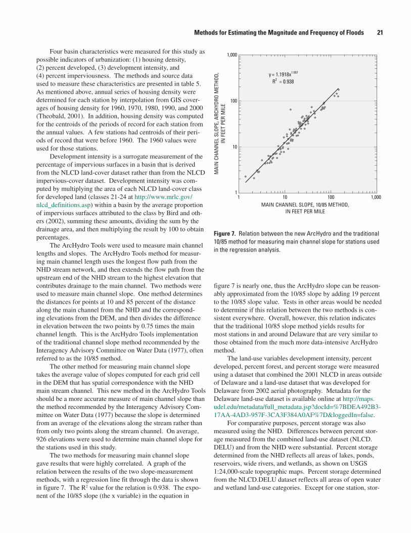
Four basin characteristics were measured for this study as possible indicators of urbanization: (1) housing density, (2) percent developed, (3) development intensity, and (4) percent imperviousness. The methods and source data used to measure these characteristics are presented in table 5. As mentioned above, annual series of housing density were determined for each station by interpolation from GIS cover-ages of housing density for 1960, 1970, 1980, 1990, and 2000 (Theobald, 2001). In addition, housing density was computed for the centroids of the periods of record for each station from the annual values. A few stations had centroids of their peri-ods of record that were before 1960. The 1960 values were used for those stations.
Development intensity is a surrogate measurement of the percentage of impervious surfaces in a basin that is derived from the NLCD land-cover dataset rather than from the NLCD impervious-cover dataset. Development intensity was com-puted by multiplying the area of each NLCD land-cover class for developed land (classes 21-24 at http://www.mrlc.gov/nlcd_definitions.asp) within a basin by the average proportion of impervious surfaces attributed to the class by Bird and oth-ers (2002), summing these amounts, dividing the sum by the drainage area, and then multiplying the result by 100 to obtain percentages.
The ArcHydro Tools were used to measure main channel lengths and slopes. The ArcHydro Tools method for measur-ing main channel length uses the longest flow path from the NHD stream network, and then extends the flow path from the upstream end of the NHD stream to the highest elevation that contributes drainage to the main channel. Two methods were used to measure main channel slope. One method determines the distances for points at 10 and 85 percent of the distance along the main channel from the NHD and the correspond-ing elevations from the DEM, and then divides the difference in elevation between the two points by 0.75 times the main channel length. This is the ArcHydro Tools implementation of the traditional channel slope method recommended by the Interagency Advisory Committee on Water Data (1977), often referred to as the 10/85 method.
The other method for measuring main channel slope takes the average value of slopes computed for each grid cell in the DEM that has spatial correspondence with the NHD main stream channel. This new method in the ArcHydro Tools should be a more accurate measure of main channel slope than the method recommended by the Interagency Advisory Com-mittee on Water Data (1977) because the slope is determined from an average of the elevations along the stream rather than from only two points along the stream channel. On average, 926 elevations were used to determine main channel slope for the stations used in this study.
The two methods for measuring main channel slope gave results that were highly correlated. A graph of the relation between the results of the two slope-measurement methods, with a regression line fit through the data is shown in figure 7. The R2 value for the relation is 0.938. The expo-nent of the 10/85 slope (the x variable) in the equation in
figure 7 is nearly one, thus the ArcHydro slope can be reason-ably approximated from the 10/85 slope by adding 19 percent to the 10/85 slope value. Tests in other areas would be needed to determine if this relation between the two methods is con-sistent everywhere. Overall, however, this relation indicates that the traditional 10/85 slope method yields results for most stations in and around Delaware that are very similar to those obtained from the much more data-intensive ArcHydro method.
The land-use variables development intensity, percent developed, percent forest, and percent storage were measured using a dataset that combined the 2001 NLCD in areas outside of Delaware and a land-use dataset that was developed for Delaware from 2002 aerial photography. Metadata for the Delaware land-use dataset is available online at http://maps.udel.edu/metadata/full_metadata.jsp?docId=%7BDEA492B3-17AA-4AD3-957F-3CA3F384A0AF%7D&loggedIn=false.
For comparative purposes, percent storage was also measured using the NHD. Differences between percent stor-age measured from the combined land-use dataset (NLCD.DELU) and from the NHD were substantial. Percent storage determined from the NHD reflects all areas of lakes, ponds, reservoirs, wide rivers, and wetlands, as shown on USGS 1:24,000-scale topographic maps. Percent storage determined from the NLCD.DELU dataset reflects all areas of open water and wetland land-use categories. Except for one station, stor-
MAIN CHANNEL SLOPE, 10/85 METHOD,IN FEET PER MILE
MAI
NCH
ANN
ELSL
OPE,
ARCH
YDRO
MET
HOD,
INFE
ETPE
RM
ILE
1,000
100
10
11 10 100 1,000
y = 1.1918xR = 0.938
1.007
2
Figure 7. Relation between the new ArcHydro and the traditional 10/85 method for measuring main channel slope for stations used in the regression analysis.
Methods for Estimating the Magnitude and Frequency of Floods 21

age values determined from NLCD.DELU were larger than those from the NHD.
Boxplots of the two storage measurements are shown in figure 8. The boxplots show how the data are distributed (Tukey, 1977). The horizontal line inside the box shows the location of the median value. The top and bottom of the box indicate the quartiles, which are the values that are exceeded 75 and 25 percent of the time. The vertical lines extending upward and downward from the box are known as the whis-kers. They encompass all values that are within 1.5 times the length of the box (1.5 times the interquartile range). Values that are within the upper and lower whiskers are indicated in the explanation as within the upper and lower adjacent regions of the boxplots, respectively. Values that are outside the whiskers are shown individually. Values shown with an “x” in the boxplot are referred to as outside values. These values are within 3 times the interquartile range in either direction from the median. The values shown with an “o” in the boxplot are referred to as detached values. These values are more than 3 times the interquartile range in either direction from the median. The boxplots show that the 75th percentile of the NHD values is approximately equal to the 25th percentile of the NLCD.DELU values.
Percent storage values from the NLCD.DELU were much more highly correlated with flood frequencies than the values from the NHD, indicating that NLCD.DELU storage is a better individual predictor of flood frequencies than NHD storage. As discussed in the next section, however, when used in conjunction with other explanatory variables, the inclu-sion of NHD storage provided regression equations with the greater accuracy in predicting flood magnitudes of specified frequency. Correlation coefficients between the logarithms of NLCD.DELU values and the logarithms of the T-year floods ranged from -0.338 for the 2-year flood to -0.396 for the 500-year flood. Correlation coefficients for the NHD values ranged from 0.003 for the 10-year flood to -0.039 for the 500-year flood.
Much of the land area of southern Delaware has been ditched to provide drainage for agriculture. One issue of con-cern for DelDOT was that the NHD representation of streams would inadequately capture the ditches that are actually present on the landscape, and there would be errors in drain-age boundaries and basin characteristics determined for some selected streams because of this. Consequently, a GIS was used to compare the NHD streams to county-mapped ditches, and to determine if incorporation of the ditches into the NHD would be necessary. The comparison indicated that the NHD incorporated the great majority of the ditches. Some areas had ditches that were not included in the NHD, and drainage boundaries determined for these areas could be in error. In general, however, the affected areas are small (less than 1 mi2). It was determined that adding all missing ditches into the NHD would be too large a task for inclusion in this study, and it would generally provide little benefit.
Development of Regression EquationsRegression equations were developed for use in
estimating peak flows associated with the 2- through 500-year recurrence intervals at both ungaged and gaged locations for the two hydrologic regions in Delaware. All response (T-year peak flows) and explanatory variables (basin characteristics) were transformed to logarithms, base 10, prior to the regres-sion analyses to obtain linear relations between the response variables and the explanatory variables, and to achieve equal variance about the regression line. A one (1) was added to all basin characteristics given as percentages to facilitate transformation to logarithms.
Equation development was done in three phases. The first phase used weighted all-possible-subsets (APS) regres-sion methods to identify possible optimal combinations of explanatory variables. The second phase used WLS regres-sion to test the adequacy of candidate explanatory variable subsets for violations of regression analysis assumptions and to determine if separate sets of equations were needed for each physiographic region. The third phase used Estimated- Generalized-Least-Squares (EGLS) regression methods to determine the final regression equations.
EXPLANATION
75th PERCENTILE (75 percent of thedata values are less than this value.)MEDIAN
INTE
RQUA
RTIL
ERA
NGE
(IQR
)
25th PERCENTILE (25 percent of thedata values are less than this value.)MINIMUM VALUE
MAXIMUM VALUE
DETACHED VALUE (greater than 3times the IQR outside the quartile)
OUTSIDE VALUE (less than or equalto 3 times and greater than 1.5 timesthe IQR outside the quartile)
X
X
XX
XXXX
XX
PERC
ENT
STOR
AGE
40
30
20
10
0NHD NLCD.DELU
Figure 8. Percent storage measured using the National Hydrography Dataset (NHD) and a combination of the 2001 National Land Cover Dataset (NLCD) and the 2002 Delaware Land-Use Dataset (DELU).
22 Magnitude and Frequency of Floods on Nontidal Streams in Delaware

In APS regression (Neter and others, 1985, p. 421-429), all possible combinations of explanatory variables were tested to identify a small set of possible best combinations of explanatory variables for further testing with WLS regression methods. Weighting was applied in the APS regressions to correct for differences in record length by dividing the number of years of systematic data available for each station by the mean record length for all stations. As a result, stations with longer records were given greater weight in the analysis than stations with shorter records. The Mallow’s C
p criterion was
used for selecting best subset combinations (Neter and others, 1985, p. 426-428).
The WLS analyses were used for detailed testing of candidate models identified through the APS analyses. Weights used in the WLS analyses were the same as those used for the APS analyses. WLS results were examined to identify potential undesirable statistical characteristics, and to select the final combinations of variables to be included in the EGLS analysis. Possible undesirable statistical characteristics that could lead to elimination of a set of candidate explana-tory variables included (1) geographic bias of the potential equations, (2) extreme influence of flood-frequency values or high leverage of the basin characteristics for individual sta-tions, (3) high correlation (multicollinearity) among potential explanatory variables, or (4) lack of statistical significance of the explanatory variables at the 95-percent probability level. The WLS analyses indicated that developing separate sets of regression equations for the Coastal Plain and Piedmont hydrologic regions would result in more accurate relations than developing a single set of equations for the entire State.
EGLS was used to determine the final regression equations because the EGLS algorithm is able to assign weights to the stations used in the analysis to adjust not only for differences in record length, as in WLS, but also for cross-correlation of the annual time series on which the peak-flow statistics for the stations are based, and for spatial correlation among the stations (Stedinger and Tasker, 1985). Because the WLS and EGLS weighting schemes were not the same, it was necessary to test several combinations of explanatory variables identified through the APS/WLS process to determine the best EGLS equations for the 2- through 500-year recurrence inter-vals in each of the two hydrologic regions. The combinations of explanatory variables that met all requirements with regard to leverage, influence, and multicollinearity while also provid-ing the lowest estimation error for each recurrence interval in each region, were selected for inclusion in the final regression equations.
The results of the analyses described above are separate sets of the best regression equations for the Piedmont and Coastal Plain regions, which can be used to estimate peak flows of known accuracy with recurrence intervals between 2 and 500 years for gaged and ungaged streams in Delaware. The final equations were developed for the Piedmont using 47 stations, and for the Coastal Plain using 55 stations. Four-teen sites that were considered for use were excluded from regression equation development—7 with unadjustable trends
in their annual peak-flow series, 5 that are in close proxim-ity on the same stream to sites that were included, and 2 that exerted undue leverage on the form of the regression equa-tions caused by basin characteristic values that are atypical of streams in Delaware. The best equations are as follows:
Piedmont region
PK2 = 1,320DRNAREA0.684(FOREST+1)-0.540(SOILA+1)-0.219
(IMPNLCD01+1)0.101 (2)
PK5 = 3,080DRNAREA 0.662(FOREST +1)-0.568(SOILA+1)-0.224 (3)
PK10 = 2,190DRNAREA 0.674(FOREST +1)-0.447(STORNHD+1)-0.346 (4)
PK25 = 2,580DRNAREA 0.675(FOREST +1)-0.391(STORNHD+1)-0.445 (5)
PK50 = 2,840DRNAREA 0.679(FOREST +1)-0.353(STORNHD+1)-0.520 (6)
PK100 = 3,090DRNAREA 0.684(FOREST +1)-0.316(STORNHD+1)-0.594 (7)
PK200 = 3,310DRNAREA 0.689(FOREST +1)-0.282(STORNHD+1)-0.668 (8)
PK500 = 3,600DRNAREA 0.698(FOREST +1)-0.239(STORNHD+1)-0.765 (9)
Coastal Plain region
PK2 = 92.8DRNAREA 0.710BSLDEM10M 0.303(SOILA+1)-0.301 (10)
PK5 = 157DRNAREA 0.710BSLDEM10M 0.292(SOILA+1)-0.310 (11)
PK10 = 210DRNAREA 0.709BSLDEM10M 0.289(SOILA+1)-0.316 (12)
PK25 = 288DRNAREA 0.711BSLDEM10M0.292(SOILA+1)-0.323 (13)
PK50 = 353DRNAREA 0.712BSLDEM10M0.297(SOILA+1)-0.328 (14)
PK100 = 425DRNAREA 0.715BSLDEM10M0.303(SOILA+1)-0.332 (15)
PK200= 505DRNAREA 0.717BSLDEM10M0.310(SOILA+1)-0.337 (16)
PK500 = 623DRNAREA 0.720BSLDEM10M0.320(SOILA+1)-0.344 (17)
Methods for Estimating the Magnitude and Frequency of Floods 23

where
PK2, PK5,…, PK500 are the peak discharges for floods with recurrence intervals of 2 years, 5
years,…, 500 years, in ft3/s;
DRNAREA is the drainage area, in mi2;
FOREST is percent forest;
IMPNLCD01 is percent impervious determined from the 2001 NLCD impervious dataset;
STORNHD is percent storage from NHD, in percent;
BSLDEM10M is mean basin slope determined from a 10-m DEM, in percent, and;
SOILA is hydrologic soil type A, in percent, high infiltration-rate soils.
The methods and source data used to calculate the variables in equations (2) through (17) are identified in table 5. Discharge estimates calculated by use of the equations are in units of cubic feet per second, but they may be converted to other measurement systems by applying the appropriate conversion factor. Systematic record, regres-sion equation, and weighted estimates of the flood-frequency statistics for each station considered for use in the regression analyses are shown in table 8. The method for determining the weighted estimates is described below.
Normally, allowing the equation for each recurrence interval to contain the best variables for estimating flood discharge for that interval without regard to variables used for other recurrence intervals improves the accuracy of the equa-tions. The drawback to this approach, however, is that equa-tions that contain different variables for successive recurrence intervals may provide estimated discharge magnitudes that do not increase with increasing recurrence interval. The 2-year recurrence interval flood discharge estimate for a particular site may be larger than the 5-year estimate for the same site, for example.
The initial set of best equations developed for each region had explanatory variables that differed among the recurrence intervals. Tests of these equations indicated a high incidence of estimated flood flows that did not increase with increasing recurrence interval. To avoid these irregularities, the housing density explanatory variable that was found significant for the 2-, 5-, and 10-year recurrence intervals for the Coastal Plain was replaced by the mean basin slope explanatory variable for these recurrence intervals to avoid reductions in flow between the 10- and 25-year recurrence intervals when housing density was included in the equations. Dropping of housing density from the Coastal Plain equations lowered the accuracy of the affected equations somewhat, but eliminated irregularities in estimated flows with increasing recurrence intervals.
The percent storage explanatory variable was allowed to remain in the equation for estimating the 10-year peak
discharge for the Piedmont, and the percent forest explanatory variable was allowed to remain in the equation for estimat-ing the 500-year peak discharge for the Piedmont region even though their statistical significance in the relations did not meet the standard criterion used for variable selection. These substitutions of variables reduced irregularities in the estimated flows with increasing recurrence intervals, but some irregularities can still occur between flow estimates for the 5- and 10-year recurrence intervals when the percent forest for an ungaged site is less than about 15 percent.
Accuracy and LimitationsThe accuracy of a regression equation depends on the
model error and the sampling error. Model error measures the ability of a set of explanatory variables to estimate the values of peak-flow characteristics calculated from the station records used to develop the equation. Sampling error measures the ability of a finite number of stations with a finite number of recorded annual peak flows to describe the true peak-flow characteristics of the entire peak-flow record for a station. Model error depends on the number and predictive power of the explanatory variables in a regression equation. Sampling error depends on the number and record length of stations used in the analysis, and decreases as the number of stations and record lengths increases.
Traditional measures of the accuracy of peak-discharge regression equations are the standard errors of estimate and prediction, and the equivalent years of record. The standard error of estimate is derived from the model error, and is a measure of how well the estimated peak discharges generated using an equation agree with the peak-flow statistics gener-ated from station records that were used to create the equation. Approximately two thirds of the estimates obtained from the equations for the stations used in the regression analysis have errors less than the noted standard errors of estimate. The standard error of prediction is derived from the sum of the model error and the sampling error, and is a measure of how accurately the estimated peak discharges generated using an equation will be able to predict the true value of peak dis-charge for the selected recurrence interval. Approximately two thirds of the estimates obtained from the equations for ungaged sites will have errors less than than the noted stan-dard errors of prediction. The equivalent years of record is an estimate of the number of years of station record that would be needed at a given ungaged site to produce peak-discharge estimates with an accuracy equal to that of the associated regression equation. The equivalent years of record is derived from a relation between the standard error of estimate and the measure of variability of the observed peak discharges used to develop an equation. Average standard errors of estimate and prediction and equivalent years of record associated with equations (2) through (17) are shown in table 9.
Prediction intervals are another useful indicator of the uncertainty inherent in use of the regression equations when applied to ungaged sites. A prediction interval is given as a
�� Magnitude and Frequency of Floods on Nontidal Streams in Delaware

minimum and maximum value within which there is a stated probability that the true value of the response variable exists. As an example, the minimum and maximum values given in a 90-percent prediction interval for the 100-year peak for an ungaged site should be interpreted to mean that there is 90-percent confidence that the true value of the 100-year peak is within the prediction interval.
Tasker and Driver (1988) have shown that a 100(1- α) prediction interval for the true value of a streamflow statistic obtained for an ungaged site from a regression equation can be computed by
Q/T < Q < TQ (18)
where
Q
is the streamflow statistic for the site and T is computed as:
(19)
In equation (19), t(α / 2,n-p) is the critical value from the
students t-distribution at alpha-level α (α = 0.10 for 90-percent prediction intervals); n-p is the degrees of freedom with n sta-tions (n=55 for the Coastal Plain and n=47 for the Piedmont) used in the regression analysis and p parameters in the equa-tion (the number of basin characteristics plus one); and S
i is
computed from equation (20) below. Critical values from the students t-distribution are contained in many introductory sta-tistics textbooks. Other prediction intervals can be calculated by changing α to obtain the desired percentage.
The value of Si is computed using the equation
(20)
where
γ2 is the model error variance;
xi is a row vector of the logarithms of the basin characteristics for site i, augmented by a 1 as the first element;
U is the covariance matrix for the regression coefficients; and
xi´ is the transpose of xi (Ludwig and Tasker, 1993).
The values of t(α / 2,n-p)
,γ2, and U needed to determine prediction intervals for estimates obtained from the regression equations are presented in table 10.
The procedure necessary to obtain the estimates is explained below with an example computation of the 50-year peak discharge for a hypothetical ungaged site on the Christina River near Newark, Delaware. First, the necessary basin char-acteristics for the site are measured from the various GIS data layers. Values for drainage area, percent forest, and percent storage are 8.00 mi2, 30.00 percent, and 0.60 percent, respec-tively. Substituting these values into equation (6) to predict the 50-year peak discharge yields
PK50 = 2,840(8.00)0.679(30.00+1)-0.353(0.60+1)-0.520=2,720 ft3/s.
Table �. Average standard errors of estimate and prediction and equivalent years of record for the best regression equations, by hydrologic region in Delaware.
Recurrence interval (years)
Piedmont Coastal Plain
Average standard errors Equivalent years of record (years)
Average standard errors Equivalent years of record (years)
Estimate (percent)
Prediction (percent)
Estimate (percent)
Prediction (percent)
2 26.6 28.9 4.1 64.3 67.4 0.8
5 26.0 28.1 6.7 57.1 60.1 1.6
10 27.4 29.9 8.4 55.3 58.5 2.4
25 28.3 31.0 11.3 55.5 59.0 3.5
50 29.8 32.7 12.7 57.0 60.8 4.2
100 31.8 35.1 13.5 59.3 63.4 4.8
200 34.4 38.0 13.8 62.4 66.9 5.2
500 38.2 48.3 13.7 67.3 72.3 5.6
ipn StT ,2/10
5.02
iii UxxS
Methods for Estimating the Magnitude and Frequency of Floods ��

Table 10. Values needed to determine 90-percent prediction intervals for the best regression equations, by hydrologic region in Delaware.
[t, the critical value from the Student’s t distribution used in equation 19; 2, the regression model error variance used in equation 20; U, the covariance matrix used in equation 20]
Piedmont
Recurrence interval (years)
t γ2 U
2 1.682 0.0129 0.032399 0.000256 -0.015862 -0.008039 -0.006372
0.000256 0.001094 -0.000897 -0.000551 -0.000209
-0.015862 -0.000897 0.009974 0.002040 0.002671
-0.008039 -0.000551 0.002040 0.007052 0.001515
-0.006372 -0.000209 0.002671 0.001515 0.002657
5 1.681 0.0123 0.018606 -0.000293 -0.010122 -0.004813
-0.000293 0.001139 -0.000715 -0.000458
-0.010122 -0.000715 0.007731 0.000596
-0.004813 -0.000458 0.000596 0.006605
10 1.681 0.0137 0.020045 -0.001710 -0.013381 0.008815
-0.001710 0.001841 0.000092 -0.004745
-0.013381 0.000092 0.010790 -0.008049
0.008815 -0.004745 -0.008049 0.042291
25 1.681 0.0145 0.023753 -0.001963 -0.015881 0.010301
-0.001963 0.002131 0.000089 -0.005454
-0.015881 0.000089 0.012815 -0.009442
0.010301 -0.005454 -0.009442 0.048422
50 1.681 0.0160 0.027642 -0.002241 -0.018531 0.011950
-0.002241 0.002448 0.000097 -0.006257
-0.018531 0.000097 0.014957 -0.010975
0.011950 -0.006257 -0.010975 0.055508
100 1.681 0.0182 0.032334 -0.002587 -0.021740 0.013985
-0.002587 0.002836 0.000116 -0.007254
-0.021740 0.000116 0.017545 -0.012862
0.013985 -0.007254 -0.012862 0.064376
200 1.681 0.0211 0.037763 -0.002997 -0.025458 0.016371
-0.002997 0.003289 0.000146 -0.008428
-0.025458 0.000146 0.020538 -0.015074
0.016371 -0.008428 -0.015074 0.074865
500 1.681 0.0257 0.045988 -0.003629 -0.031101 0.020027
-0.003629 0.003980 0.000202 -0.010230
-0.031101 0.000202 0.025073 -0.018465
0.020027 -0.010230 -0.018465 0.091042
�� Magnitude and Frequency of Floods on Nontidal Streams in Delaware

Table 10. Values needed to determine 90-percent prediction intervals for the best regression equations, by hydrologic region in Delaware.—Continued
[t, the critical value from the Student’s t distribution used in equation 19; 2, the regression model error variance used in equation 20; U, the covariance matrix used in equation 20]
Coastal Plain
Recurrence interval (years)
t γ2 U
2 1.675 0.0652 0.014305 -0.004551 -0.004712 -0.008147
-0.004551 0.004659 0.000261 -0.000044
-0.004712 0.000261 0.017005 0.004016
-0.008147 -0.000044 0.004016 0.008181
5 1.675 0.0532 0.012706 -0.004072 -0.004172 -0.006940
-0.004072 0.004069 0.000284 -0.000062
-0.004172 0.000284 0.015025 0.003457
-0.006940 -0.000062 0.003457 0.007005
10 1.675 0.0504 0.012851 -0.004115 -0.004178 -0.006867
-0.004115 0.004068 0.000294 -0.000086
-0.004178 0.000294 0.015252 0.003446
-0.006867 -0.000086 0.003446 0.006968
25 1.675 0.0507 0.013878 -0.004422 -0.007297 -0.004438
-0.004422 0.004344 -0.000127 0.000296
-0.007297 -0.000127 0.007454 0.003690
-0.004438 0.000296 0.003690 0.016605
50 1.675 0.0531 0.015112 -0.004793 -0.007900 -0.004777
-0.004793 0.004705 -0.000163 0.000297
-0.007900 -0.000163 0.008105 0.004010
-0.004777 0.000297 0.004010 0.018187
100 1.675 0.0569 0.016674 -0.005268 -0.008696 -0.005222
-0.005268 0.005176 -0.000203 0.000300
-0.008696 -0.000203 0.008952 0.004426
-0.005222 0.000300 0.004426 0.020161
200 1.675 0.0620 0.018532 -0.005839 -0.009660 -0.005764
-0.005839 0.005746 -0.000247 0.000307
-0.009660 -0.000247 0.009972 0.004926
-0.005764 0.000307 0.004926 0.022483
500 1.675 0.0704 0.021407 -0.006729 -0.011172 -0.006618
-0.006729 0.006640 -0.000311 0.000323
-0.011172 -0.000311 0.011562 0.005705
-0.006618 0.000323 0.005705 0.026044
Methods for Estimating the Magnitude and Frequency of Floods ��

To determine a 90-percent prediction interval for this estimate, the xi vector is
xi = {1, log
10(8.00). log
10(31.00), log
10(1.60)}
the model error variance from table 10 is γ2 = 0.0160, and the covariance matrix, U, for the 50-year peak discharge in the Piedmont hydrologic region is
The standard error of prediction computed using equation (20) is S
i=(0.0160+0.00205)^0.5=0.1344, and T
computed from equation (19) is T=10^(1.681*0.1344)=1.682. The 90-percent prediction interval is estimated from equa-tion (18) as (2,720/1.682)< PK50<(2,720*1.682), or, 1,620< PK50< 4,580.
The regression equations can be used to estimate peak-flow frequencies for ungaged sites with natural flow condi-tions in Delaware. The equations should not be applied to streams with substantial flood-retention storage upstream from sites of interest.
The accuracy of the equations is known only within the range of the basin characteristics used to develop the equa-tions. The equations can be applied for ungaged sites with basin characteristics that are not within the ranges of appli-
cability, but the accuracy of the estimates will be unknown. Also, it is possible that discharge estimates for lower-recur-rence-interval floods can be larger than discharge estimates for higher-recurrence-interval floods when basin character-istics for an ungaged site are substantially beyond the ranges of applicability. The ranges of basin characteristics used to develop the equations are provided in table 11.
Comparison of Results with Previous StudyA comparison was made between estimates obtained
from the systematic records and the regression equations in this report and those from the previous Delaware flood- frequency report (Dillow, 1996) for stations that were used in both reports. Mean and median percent differences between the flood-frequency estimates obtained from the systematic record from the previous study and from this study were com-puted for all stations and by region, and are shown in table 12. Differences for the 200-year recurrence interval are not shown in the table because discharges for this recurrence interval were not computed for the previous study.
Estimates determined from the systematic record for this study are, on average, larger in discharge than those from the previous study for the lowest recurrence intervals, and they are smaller than those from the previous study for the high-est recurrence intervals when all stations are considered as a group. Mean differences in percent range from positive 9.9 percent for the 2-year recurrence interval to negative 18.5 percent for the 500-year recurrence interval. Median
Table 11. Ranges of basin characteristics used to develop the regression equations.
[NHD, National Hydrography Dataset]
Piedmont region Coastal Plain region
Basin characteristic Minimum Maximum Minimum Maximum
Drainage area (square miles)
0.31 319 0.51 117
Forest cover (percent)
4.07 84.9 -- --
Impervious area (percent)
0.10 38.3 -- --
Storage (NHD) (percent)
0.00 2.92 -- --
Housing density (homes/acre)
0.06 6.84 0.01 3.42
Hydrologic soil type A (percent)
0.00 7.22 0.53 60.0
Mean basin slope (percent)
-- -- 0.30 3.69
0.027642 -0.002241 -0.018531 0.011950
U = -0.002241 0.002448 0.000097 -0.006257
-0.018531 0.000097 0.014957 -0.010975
0.011950 -0.006257 -0.010975 0.055508
�� Magnitude and Frequency of Floods on Nontidal Streams in Delaware

differences in percent range from positive 2.9 percent for the 2-year recurrence interval to negative 22.3 percent for the 500-year recurrence interval. Many stations within the study area experienced major flooding since completion of the previous study, which could lead to the expectation that flood-frequency estimates would increase rather than decrease. The decrease in the higher recurrence-interval estimates, however, can mostly be explained by (1) additional record for many of the stations, (2) the improved generalized-skew values used for this study, which are substantially lower than the previous val-ues taken from Bulletin 17B, and account for lowering of the 100-year peaks by an average of about 4 percent, (3) the use of more historical adjustments than were used for the previous study, and (4) adjustments for trends in the annual peak-flow time series at some stations.
As indicated in table 12, differences between the estimates from the previous and current studies vary substan-tially depending on the region and whether or not additional data were collected. When all stations are considered, percent differences generally are much larger in the Coastal Plain than in the Piedmont, and stations with no record since the previous study have very small positive mean changes for smaller peaks and large negative mean changes for larger peaks, whereas sta-tions with additional record since the previous study have large positive mean changes for smaller peaks and small negative mean changes for larger peaks. For the Coastal Plain, stations with no additional record have small negative mean changes for smaller peaks and large negative mean changes for larger peaks, whereas stations with additional record have large positive mean changes for smaller peaks and large
Table 1�. Mean and median percent differences between peak-flow frequency statistics computed from the systematic records for streamgaging stations included in this study and the previous study (Dillow, 1996).
Recurrence interval
All stations Coastal Plain Piedmont
Mean percent
difference
Median percent
difference
Mean percent
difference
Median percent
difference
Mean percent
difference
Median percent
difference
All stations
2 9.9 2.9 16.0 2.9 4.7 2.8
5 3.5 1.4 3.4 -0.7 3.7 1.9
10 -0.9 -1.5 -3.8 -6.5 1.9 -1.0
25 -5.9 -5.9 -11.2 -8.4 -0.6 -4.7
50 -9.5 -9.3 -16.2 -14.0 -2.6 -8.3
100 -12.6 -13.6 -20.5 -18.6 -4.5 -13.1
500 -18.5 -22.3 -28.8 -30.1 -8.0 -20.5
Stations with no record since last study
2 0.9 2.9 -2.4 -2.1 4.2 3.2
5 -4.7 1.4 -11.1 -10.5 1.8 0.7
10 -9.1 -1.5 -16.8 -12.4 -1.5 -2.4
25 -14.6 -5.9 -23.0 -17.7 -6.2 -6.3
50 -18.9 -9.3 -27.3 -23.6 -10.6 -9.8
100 -22.8 -13.6 -31.0 -29.7 -14.5 -14.0
500 -31.0 -22.3 -38.5 -41.4 -23.4 -22.3
Stations with additional record since last study
2 24.3 6.7 48.1 13.4 5.7 2.3
5 14.6 7.8 27.0 13.4 4.9 5.4
10 9.5 6.6 16.6 11.5 4.0 2.7
25 4.5 2.7 6.5 7.6 2.9 -1.7
50 1.4 -3.3 0.0 -3.3 2.5 -5.2
100 -1.1 -8.8 -5.3 -8.8 2.2 -9.0
500 -4.9 -17.4 -15.2 -20.1 3.2 -17.4
Methods for Estimating the Magnitude and Frequency of Floods ��

negative mean changes for larger peaks. For the Piedmont, stations with no additional record have small positive mean changes for smaller peaks and large negative mean changes for larger peaks, whereas stations with additional record have small positive mean changes for all peaks.
Adjustments for trends for some stations also contribute to increasing the low recurrence-interval estimates and decreasing the high recurrence-interval esti-mates. Because the annual peak flows tend to be smaller for the trend-affected stations during earlier parts of the periods of record than during later parts, the trend adjustments gener-ally have the effect of increasing the lower flows more than the higher flows, and lowering the standard deviations of the annual series. This results in higher discharge estimates for the lower recurrence intervals and lower discharge estimates for the higher recurrence intervals.
Errors associated with the regression equations cannot be directly compared between the two studies because the same stations and explanatory variables were not used; how-ever, some comparison is justified to understand differences between the results. Average standard errors of prediction associated with the regression equations for the Piedmont are somewhat larger for this study (28 to 48 percent) than for the previous study (23 to 45 percent). Average standard errors of prediction associated with the regression equations for the Coastal Plain are substantially larger for this study (58 to 72 percent) than for the previous study (38 to 43 percent).
The large differences in error between the two studies were not expected and they cannot be fully explained, but it is likely that the new average standard errors of prediction give a more precise indication of the true errors associated with estimates from the regression equations than the average stan-dard errors of prediction given for the previous equations. The regression methods used in the two studies were essentially the same. The peak-flow statistics for the stations used in this study are considered more precise than those used in the previ-ous study because of (1) improved generalized-skew values, (2) longer periods of record for many stations, and (3) correc-tions for trends that were not made previously. In addition, the basin characteristics used as explanatory variables in the equations were generally measured with more precision than those from the previous study.
A possible explanation for the increased error in the equa-tions is that many of the long-term streamgaging stations used in the analysis have experienced large peaks since the previous study was completed. These large peaks may have increased the uncertainty in systematic flood-frequency estimates used as the dependent variables in the regression analyses. Percent differences in discharge between estimates obtained from the previous study and this study, as shown in table 12, are larger for the Coastal Plain, where average standard errors of estimate have increased the most, than for the Piedmont. The Coastal Plain also has the largest differences between the per-cent changes for stations with and without additional record. The pattern of changes for the Coastal Plain stations with and
without new record is substantially different, indicating that more recent events are causing the differences in the changes.
This study included 21 stations in the Coastal Plain of southern New Jersey that were not included in the previ-ous study. There was some concern that differences in the physiography of southern New Jersey and the Coastal Plain in Delaware were large enough that the addition of the New Jersey stations was causing the increased errors. A test set of regression analyses was run excluding the New Jersey stations. Average prediction errors decreased a few percentage points when this was done, but the decision was made to include the New Jersey stations in the final analyses to extend the range of applicability of the resulting regression equations.
Application of the MethodsThe best estimates of flood frequencies for a site are
often obtained through a weighted combination of estimates produced from more than one method. Tasker (1975) dem-onstrated that if two independent estimates of a streamflow statistic are available, a properly weighted average of the independent estimates will provide an estimate that is more accurate than either of the independent estimates. Improved flood-frequency estimates can be determined for Delaware streamgaging stations by weighting estimates determined from the systematic peak-flow record at the station with estimates obtained from the regression equations provided in this report. Improved estimates can be determined for ungaged sites in Delaware by weighting the estimates obtained from the regres-sion equations with estimates determined based on the flow per unit area of an upstream or downstream streamgaging station.
The sections below describe the weighting process for streamgaging stations and ungaged sites in more detail, and provide example calculations. The methods presented are those incorporated into the USGS National Flood Frequency Program (NFF) (Ries and Crouse, 2002), a computer program that can be used to solve all of the USGS flood-frequency equations in the Nation, including those from this report, given user input of basin characteristics. NFF can be downloaded from the web at http://water.usgs.gov/software/nff.html, along with complete documentation on how to use it. NFF can also be used to perform the weighting functions described below for estimation at a gaged location and for an ungaged site upstream or downstream from a gaged location, but not for an ungaged site between gaged locations. The StreamStats program (described later in the StreamStats section) does not currently (2006) include the weighting functionality that is in NFF.
30 Magnitude and Frequency of Floods on Nontidal Streams in Delaware

Estimation for a Gaged Location
The Interagency Advisory Committee on Water Data (1982) recommends that the best estimates of flood-fre-quency statistics for a streamgaging station can be obtained by combining the estimates determined from log-Pearson type III analysis of the systematic annual peaks with estimates obtained for the station from regression equations. Note that the symbols used to explain this method in the source publica-tion have been preserved in the discussion below, and that the equivalent expressions used in this report are identified in the variable definitions that accompany each equation.
Weighting is based on the years of record for the esti-mates obtained from the station records and on the equivalent years of record for the regression estimates. If the two differ-ent estimates are assumed to be independent, weighted flood-frequency estimates can be computed as
(21)
where
QT(G)w
is the weighted estimate of flood-peak discharge for any recurrence interval (PK2, PK5, ...,PK500) at the streamgaging station,
QT(G)s
is the estimate of (PK2, PK5,…, PK500) derived from the systematic flood peaks,
QT(G)r
is the estimate of (PK2, PK5,…, PK500) derived from the regression equation,
N is the number of years of gaged record, and
EQ is the equivalent years of record determined for the regression equation.
The accuracy of the weighted estimate, in equivalent years of record, EQ
T(G)w, is equal to the N + EQ. No other indi-
cators of accuracy are available for these weighted estimates.An example of the application of the procedure described
above is the computation of the weighted 100-year flood-peak discharge for the site on Little Mill Creek at Elsmere, Delaware (station number 01480100):
1. Obtain the estimate of the 100-year discharge at the site based on the systematic flood peaks from table 8; PK100
(G)s = 6,370 ft3/s,
2. Obtain drainage area, percent forest, and percent storage from table 7, and the number of years of gaged record from table 1; DRNAREA=6.67 mi2, FOREST= 13.76 percent, STORNHD=0.35 percent, and N=18 years,
3. Compute PK100 (G)r
= 3,090(6.67)0.684(13.76+1)-0.316
(0.35+1)-0.594 =4,040 ft3/s,4. Obtain the equivalent years of record for the 100-year
peak-discharge regression equation for the Piedmont
region from table 9; EQ=13.5 years, and5. Compute the weighted 100-year flood-peak discharge for
the site; log PK100
(G)w=((18)(log6,370)+(13.5)(log4,040))/
(18+13.5)=3.7194, and PK100 (G)w
=5,240 ft3/s.
Estimation for a Site Upstream or Downstream from a Gaged Location
Guimaraes and Bohman (1992) and Stamey and Hess (1993) presented the following method to improve flood- frequency estimates for an ungaged site with a drainage area that is between 0.5 and 1.5 times the drainage area of a streamgaging station that is on the same stream. As in the previous section, the symbols used to explain this method in the source publications have been preserved in the discus-sion below, and the equivalent expressions used in this report are identified in the variable definitions that accompany each equation.
To obtain a weighted peak-flow estimate (QT(U)w
) for recurrence interval T at the ungaged site, the weighted flow estimate for an upstream or downstream streamgaging station (Q
T(G)w) must first be determined using the equation provided
in the previous section. The weighted streamgaging station estimate is then used to obtain an estimate for the ungaged site that is based on the flow per unit area at the streamgaging station (Q
T(U)g) by use of the equation
(22)
where
Au is the drainage area (DRNAREA
u) for the
ungaged site,
Ag is the drainage area (DRNAREA
g) for the
upstream or downstream streamgaging station, and
b is 0.60 in the Piedmont and 0.70 in the Coastal Plain, as determined by computing the mean of the drainage-area exponents for all recurrence intervals from regressions of flood-frequencies against drainage area as the only explanatory variable, and where the equation constant is forced to be zero.
The weighted estimate for the ungaged site (QT(U)w
) is then computed as
(23)
EQNQEQQN
Q rGTsGTwGT
)()(
)(
logloglog
wGT
b
gUT QAgAuQ )()(
gUTg
rUTg
wUT QAAQ
AAQ )()()(
212
Application of the Methods �1

where
∆A is the absolute value of the difference between the drainage areas of the streamgaging station and the ungaged site, |DRNAREA
g -
DRNAREAu|, and
QT(U)r
is the peak-flow estimate for recurrence interval (PK2, PK5,…,PK500) at the ungaged site derived from the applicable regional equation given above.
Use of the equations above gives full weight to the regression estimates when the drainage area for the ungaged site is less than 0.5 or greater than 1.5 times the drainage area for the streamgaging station, and increasing weight to the streamgaging-station-based estimates as the drainage area ratio approaches 1. The weighting procedure should not be applied when the drainage area ratio for the ungaged site and streamgaging station is less than 0.5 or greater than 1.5.
The equivalent years of record for the weighted estimate for an ungaged site, EQ
T(U)w, can be computed. This
is done by first substituting the equivalent years of record for the weighted estimate of peak discharge at the streamgaging station, EQ
T(G)w, in place of Q
T(G)w in equation (22) above to
obtain an estimate of the weighted equivalent years of record for the streamgaging station that is adjusted to the drainage area for the ungaged site, EQ
T(U)g. As noted above, EQ
T(G)w
is equal to N + EQ from equation (21). The area-adjusted equivalent years of record based on the gaged site, EQ
T(U)g, is
then substituted for QT(U)g
, and the equivalent years of record for the ungaged site based on the regression equation, EQ
T(U)r,
is substituted for QT(U)r
in equation (23) to compute the final weighted equivalent years of record for the ungaged site, EQ
T(U)w. No other indicators of accuracy are available for these
estimates. In theory, the standard errors for these estimates should be at least as small as those for the estimates derived from the regression equations alone.
An example of the application of the procedure described above is the computation of the weighted 100-year flood-peak discharge, and its associated equivalent years of record, for a hypothetical site on Little Mill Creek located above the USGS station at Elsmere, Delaware (station number 01480100) cited in the previous section:
Calculate the value of PK100(G)w
(see example in previous section); PK100
(G)w=5,240 ft3/s,
Obtain the drainage areas for both the gaged and ungaged sites; DRNAREA
g =6.67 mi2, and DRNAREA
u=4.44 mi2,
Use equation (22) and b=0.6 for stations in the Piedmont, to calculate the 100-year peak discharge based on station data; PK100
(U)g = (4.44/6.67)0.6(5,240) = 4,100 ft3/s,
Compute ∆A, where ∆A=6.67-4.44=2.23 mi2,
Compute PK100(U)r
for the ungaged site using equation (7) with FOREST= 8.00 percent and STORNHD=
1.
2.
3.
4.
5.
0.10 percent; PK100(U)r
=3,090(4.44)0.684(8.00+1)-0.316
(0.10+1)-0.594=4,040 ft3/s,
Compute the weighted estimate for the ungaged site, Q
T(U)w, using equation (23);
PK100(U)w
=[((2*2.23)/6.67)*4,040]+[(1-((2*2.23)/6.67))*3,490]=3,860 ft3/s, and finally,
Compute the equivalent years of record for the weighted estimate of the 100-year peak discharge for the ungaged site using equations (22) and (23) and substituting EQ
T(G)w
in place of QT(G)w
, EQT(U)g
, in place of QT(U)g
, EQT(U)r
in place of Q
T(U)r, and EQ
T(U)w in place of Q
T(U)w; giving:
From equation (22), EQ
100(U)g=(4.44/6.67)0.6(31.5)=
24.7 years, From table 9, EQ
100(U)r=13.5 years, and
From equation (23), EQ100(U)w
=[((2*2.23)/6.67)*13.5]+ [(1-((2*2.23)/6.67))*18]=15.0 years.
Estimation for a Site Between Gaged Locations
In the case where a flood-frequency estimate is needed for a site that is located between two gaged locations on a stream, the estimate may be obtained by use of the procedure presented above for calculating weighted estimates for a gaged location, with the following procedural alteration. For con-sistency, the symbology used below is the same as that used in the previous section, and the equivalent expressions used elsewhere in this report are identified in the variable defini-tions that accompany each equation.
Because the site is ungaged, a direct determination of the flow at the site for the selected recurrence interval is not possible. An interpolated value can be obtained by use of the equation:
(24)
where
Au is the drainage area (DRNAREA
u) for the
ungaged site,
Agu
is the drainage area (DRNAREAgu
) for the upstream gaged location,
Agd
is the drainage area (DRNAREAgd
) for the downstream gaged location,
QTu
is the discharge at the T-year recurrence interval (PK2, PK5,…, PK500) for the ungaged site,
QTgu
is the discharge at the T-year recurrence interval (PK2, PK5,…, PK500) for the upstream gaged location, and
6.
7.
8.
ugu
Tgu
gu
Tgu
gd
Tgd
gugd
guuTu A
AQ
AQ
AQ
AAAA
Q *]*[
�� Magnitude and Frequency of Floods on Nontidal Streams in Delaware

QTgd
is the discharge at the T-year recurrence interval (PK2, PK5,…, PK500) for the downstream gaged locations.
The value of QTu from equation (24) may be used in equation (21) in place of QT(G)s.
The value of N for use in equation (21) may be calculated by determining the arithmetically weighted average of the number of years of record for the upstream and downstream gaged locations, using the difference in the two drainage areas as the weighting factor. The calculation can be done using the equation:
(25)
where,
Au, A
gu, and A
gd are as defined immediately above, and
Nu, N
gu, and N
gd are the number of years of record for the
ungaged site and the upstream and downstream gaged locations, respectively.
The value determined for Nu from equation (25) may be inserted in place of the value of N in equation (21) to solve that equation, thus obtaining a weighted estimate of the T-year flood for the ungaged site located between an upstream and downstream gaged location.
An example of the application of the procedure described above is the computation of the weighted 5-year flood-peak discharge, and its associated equivalent years of record, for a hypothetical site on Brandywine Creek, with a drainage area of 300 mi2, percent forest of 31.60 percent and percent hydro-logic soil type A of 5.00, located between the USGS gages at Chadds Ford, Pennsylvania (station number 01481000) and Wilmington, Delaware (station number 01481500):
Use equation (24) to calculate PK5u with the
information given above, gaged drainage areas associated with the two stations from table 7, and the appropriate discharge characteristics from table 8; DRNAREA
u=300 mi2, DRNAREA
gu=288 mi2,
DRNAREAgd
=319 mi2, PK5gu
= 11,000 ft3/s, and PK5
gd=12,400 ft3/s, so PK5
u={[(300-
288)/(319-288)]*[(12,400/319)-(11,000/288)]+ (11,000/288)}*300=11,500 ft3/s,
Use equation (25) to calculate Nu,
with drainage areas as defined in the previous step and the years of record for the upstream (station number 01481000) and downstream (station number 01481500) gages as given in table 1; N
gu=84 years, and N
gd=93 years, so N
u =(93*(300.00-
288.17)+84*(318.54-300.00))/(318.54-288.17)= 87.5 years,
1.
2.
After computing the regression equation estimate for the ungaged site and determining the associated equivalent years of record from table 9, calculate the weighted peak discharge estimate of the ungaged site using equation (21) with PK5
(G)s=11,500 ft3/s, PK5
(G)r=12,400 ft3/s, N=87.5
years, and EQ=6.7 years, so log PK5 (G)w
=((87.5) (log11,500)+(6.7)(log12,400))/(87.5+ .7)=4.0630, and PK5
(G)w=11,600 ft3/s.
Effects of Urbanization on FloodsThe design of structures that can withstand future floods
and protection of life and property in floodplains in urbanizing basins requires an understanding of the effects of urbanization on flood peaks. Engineers and planners often need to consider the potential effects on streamflow of full-build-out scenarios in their design and planning efforts. The section above on the Analysis of and Adjustments for Trends in Annual Peak-Flow Time Series presents some findings on the effects of urbaniza-tion on annual flood peaks at streamgaging stations in and near Delaware. This section describes an analysis that was done to develop regression equations that could be used to estimate the effects of future development on flood frequencies.
A matrix of correlations between the logarithms of flood-frequency estimates at the 2- and 100-year recurrence intervals and the logarithms of drainage area and the measured indica-tors of urbanization for stations used in the regression analyses is presented in table 13. Correlations among the indicators of urbanization were very high. In addition, note that the cor-relations between the indicators of urbanization and the 2-year peak flow were higher than those for the 100-year peak flow. Although only the 2- and 100-year peak flows are shown in the correlation matrix for simplicity, additional tests showed that correlations with the indicators of urbanization decreased consistently with increasing recurrence interval.
Development intensity was computed for this study primarily as a basis for comparing how closely this measure of impervious surface percentage agrees with impervious percentage obtained directly from the 2001 NLCD impervi-ousness dataset. The matrix indicates that the correlation of peak flows with development intensity is less than half of the correlation with percent impervious, which has the highest individual correlation with the peak flows of the urbaniza-tion indicators. In addition, development intensity actually had slightly lower correlations with peak flows than percent developed. Development intensity was derived by applying weights to the same land-use categories as those used to com-pute percent developed. This indicates that the application of weights to the land-use categories was actually counterproduc-tive when attempting to explain more of the variation in peak flows.
Regressions of peak flows against the individual urbanization indicators had very high average standard errors of prediction. As a result, regressions that also included
3.
gugd
ugdguguugdu AA
AANAANN
)()(
Effects of Urbanization on Floods ��

drainage area as an explanatory variable were done to increase the accuracy of the equations. The combination of drainage area and centroid housing density provided the regression equations with the lowest errors. Regressions that included an indicator variable to differentiate between the Piedmont and the Coastal Plain were also tested, but the indicators were statistically insignificant. The equations that are most useful for developing scenarios of the effects of future urbanization on flood-frequency relations are:
UPK2 = 51.4DRNAREA0.798(HOMEDENS+1)1.09 (26)
UPK5 = 91.8DRNAREA0.783(HOMEDENS+1)0.950 (27)
UPK10 = 126DRNAREA0.775(HOMEDENS+1)0.870 (28)
UPK25 = 179DRNAREA0.767(HOMEDENS+1)0.780 (29)
UPK50 = 225DRNAREA0.762(HOMEDENS+1)0.719 (30)
UPK100 = 277DRNAREA0.758(HOMEDENS+1)0.663 (31)
UPK200 = 334DRNAREA0.754(HOMEDENS+1)0.611 (32)
UPK500 = 420DRNAREA0.751(HOMEDENS+1)0.546 (33)
where
UPK2 through UPK500 are the estimates of urban flood frequency for the 2- through 500-year recurrence intervals, in cubic feet per second, and HOMEDENS is the housing density, in homes per acre. Housing-density values used in the analysis were those associated with the centroid of the period of record for each station. The average standard errors of estimate and prediction and the equivalent years of record associated with the urban equations above are presented in table 14. The ranges of applicability for equations (26) through (33) are equivalent to the combined ranges for both regions given in table 11.
Table 1�. Matrix of correlations between the logarithms of flood-frequency estimates at the 2- and 100-year recurrence intervals and the logarithms of the indicators of urbanization.
�-year
peak flow100-year
peak flowDrainage
area
�000 Housing density
Centroid year
housing density
Percent impervious
Percent developed
2-year peak flow 1
100-year peak flow 0.952 1
Drainage area 0.769 0.738 1
2000 housing density 0.423 0.314 0.057 1
Centroid year housing density 0.352 0.291 0.038 0.704 1
Percent impervious 0.431 0.315 0.130 0.900 0.651 1
Percent developed 0.212 0.095 -0.013 0.822 0.512 0.817 1
Development intensity 0.194 0.076 -0.025 0.807 0.467 0.823 0.989
Table 1�. Average standard errors of estimate and prediction and equivalent years of record for the urban regression equations.
Recurrence interval (years)
Average standard errors of Equivalent years of record (years)
Estimate (percent)
Prediction (percent)
2 88.6 90.6 0.54
5 88.8 91.1 0.85
10 89.5 91.9 1.19
25 91.0 93.6 1.68
50 92.6 95.4 2.06
100 94.7 97.6 2.42
200 97.2 100 2.76
500 101 105 3.17
�� Magnitude and Frequency of Floods on Nontidal Streams in Delaware

Because the errors associated with the urban equa-tions are much higher than those for the best equations, it is recommended that the urban equations be applied only for the purpose of evaluating the effects of increased urbaniza-tion on peak flows. First, the best estimates of peak flows for a site should be determined using equations (2) through (17). Next, housing density should be determined under different land-use conditions and the different values of housing density should be applied using equations (26) through (33) to obtain estimates of peak flows for the different land-use scenarios. Finally, the percentage change between the peak-flow esti-mates for the different scenarios should be applied to the esti-mates obtained from equations (3) through (17) to obtain the best estimates of peak flows for the scenarios. These scenarios can be computed easily by using the NFF program, which includes both the best and the urban equations. Because the 2-year best equation for the Piedmont (equation 2) already contains the percent of impervious surfaces as a variable it is preferable to do build-out scenarios with the best equation for the 2-year recurrence interval for the Piedmont region rather than using equation 26 above. The urban equations can be incorporated into the methods used to develop build-out scenarios in the Coastal Plain region.
StreamStatsStreamStats is a map-based USGS web application that
makes it easy for users to obtain streamflow statistics and basin characteristics for USGS streamflow data-collection stations and ungaged sites of interest. It uses digital map data and a GIS to automatically determine the basin characteristics for ungaged sites. Ries and others (2004) provide a detailed description of the application. Although it is designed to even-tually be a national application, Streamstats is being imple-mented on a state-by-state basis, usually through cooperative funding agreements between the USGS and local partners.
StreamStats has been developed for Delaware. Users can access all of the flood-frequency statistics and basin charac-teristics published in this report for the stations used in this study by selecting a station location on the map shown in the StreamStats user interface. Users can also obtain estimates for ungaged sites in Delaware by selecting the location of a site of interest on the map.
Complete instructions for using StreamStats are provided through links on the StreamStats web site at http://streamstats.usgs.gov. The web site also provides links to (1) general limitations of the application, (2) other State applications, (3) definitions of terms, (4) answers to frequently asked ques-tions, (5) downloadable talks and other technical information about the application, (6) information that can be accessed only by USGS employees, and (7) contact information.
Due to software limitations, the StreamStats implemen-tation for Delaware does not include the ability to solve the urban equations presented above for ungaged sites.
Readers who are interested in using the urban equations can use StreamStats to obtain the basin characteristics needed to solve both the best equations and the urban equations, and they can get flood-frequency estimates based on the best equations. The basin characteristics obtained from Stream-Stats can then be used in the NFF program to obtain urban estimates for different development scenarios. StreamStats measures housing density for ungaged sites from the 2000 housing-density dataset (Theobald, 2001). Users will need to determine the appropriate housing-density values for other times.
Summary and ConclusionsThis study was done by the U.S. Geological Survey in
cooperation with the Delaware Geological Survey and the Delaware Department of Transportation. The report presents estimates of flood-frequency statistics and basin characteris-tics for 116 stations in and within 25 miles of Delaware. It also describes methods for estimating flood frequencies for streamgaging stations and for ungaged sites in Delaware.
Statistically significant upward trends were found in the annual time series of peak flows for 18 of the 116 streamgag-ing stations analyzed for this study. Additional analyses were done to determine if these trends were related to correspond-ing increases in annual maximum precipitation or housing density, or both. The analyses revealed that annual maximum precipitation has not been increasing in the study area, but sta-tistically significant relations were found between annual peak flows and corresponding annual values of housing density for 8 of the 18 stations.
Adjustments for trends in the annual peak-flow time series were made on the basis of time only for 11 of the 18 stations with significant trends before final flood-frequency analyses were completed for the stations. When compared to the original flood-frequency estimates for the trend-adjusted stations, the adjustments had the effect of increasing the magnitude of peak discharges for floods at recurrence intervals of up to 2 years, and decreasing the peak discharges for the 200- and 500-year recurrence intervals for all of the stations. Results varied for recurrence intervals between 5 and 100 years. For various reasons, the time series for seven of the trend-affected stations were not adjusted. These stations were not used in the regional flood-frequency analyses.
An analysis of station skews resulted in new general-ized-skew values defined for each of two hydrologic regions in Delaware -- the Piedmont and Coastal Plain regions. The Piedmont includes the area north of the Fall Line, in northern Delaware, and the Coastal Plain includes the area to the south. The new generalized skew values are 0.107 for the Piedmont and 0.204 for the Coastal Plain, and are substantially lower than skew values taken from Bulletin 17B for the previous flood-frequency study. These new generalized-skew values were used to determine the flood-frequency values from the
Summary and Conclusions ��

systematic records for the streamgaging stations presented in this report.
Discharge estimates determined from the systematic record for this study were, on average, larger than those from the previous study for the lowest recurrence intervals, and they were smaller than those from the previous study for the highest recurrence intervals when all stations are considered as a group. The changes are much larger in the Coastal Plain than in the Piedmont. The changes are due in large part to the longer periods of record and the improved generalized-skew values used for this study, and the adjustment of annual time series for some stations to eliminate trends.
Two sets of regression equations are presented for estimating flood discharges at the 2-, 5-, 10-, 25-, 50-, 100-, 200-, and 500-year recurrence intervals at ungaged sites in Delaware. One set of equations is the best set of regression equations that could be developed for estimating flood dis-charges in the study area. Separate sets of best equations were developed for the Coastal Plain and the Piedmont hydrologic regions. A second set of equations was developed for use in estimating the effects of urbanization on flood discharges. The explanatory variables in the best equations for the Coastal Plain include drainage area, percent of drainage basin covered by soil type A, and mean basin slope. The explanatory vari-ables in the best equations for the Piedmont include drainage area, percent of basin covered by forest, percent of basin cov-ered by impervious surfaces (2-year recurrence interval only), percent of basin covered by hydrologic soil type A (2-year and 5-year recurrence intervals), and percent storage (areas of wet-lands and waterbodies) determined from the National Hydrog-raphy Dataset (10- to 500-year recurrence intervals). The explanatory variables used in the urban equations included drainage area and housing density. The report presents the equations, indicators of the errors associated with use of the equations, and a discussion of the limitations for their use.
Average standard errors of prediction for the best regression equations ranged from 28 to 48 percent for the Piedmont, and from 58 to 72 percent for the Coastal Plain. Although they are not directly comparable because of differences in the stations used and their lengths of record, the errors associated with the new equations are higher than those presented in the previous report, which ranged from 23 to 45 percent for the Piedmont, and from 38 to 43 percent for the Coastal Plain. The differences in error cannot be fully explained, but it is likely that the new average standard errors of prediction give a more precise indication of the true errors associated with estimates from the regression equations than the average standard errors of prediction given for the previous equations. A possible explanation for the increased error in the equations is that many of the long-term streamgaging sta-tions used in the analysis have experienced large peaks since the previous study was completed. These large peaks lead to greater uncertainty in the flood-frequency estimates for the streamgaging stations used in the study.
Estimates of housing density under different land-use scenarios can be used with the urban equations to evaluate
the changes in flood magnitude as a result of the land-use changes. The average standard errors of prediction for the urban equations range from 91 to 105 percent. Consequently, these equations should be used only to compute the percentage change for different scenarios.
The best equations and the urban equations developed during this study have been incorporated into the National Flood Frequency (NFF) and StreamStats programs of the USGS. The National Flood Frequency program is a desktop program that solves regression equations for all states in the Nation, and requires user input of the basin characteristics. The StreamStats program is a web application that can provide the streamflow statistics and basin characteristics published in this report for streamgaging stations when users select a sta-tion location in the user interface. StreamStats can also com-pute basin characteristics and provide estimates of streamflow statistics for ungaged sites when users select the location of a site along any stream in Delaware.
This report describes methods for obtaining improved flood-frequency estimates for streamgaging stations and ungaged sites. Improved estimates for streamgaging stations are obtained by computing the weighted average of the esti-mates obtained from the systematic record and the estimates obtained from the regression equations, with weighting based on the years of systematic record and the equivalent years of record for the regression estimates. Improved estimates for ungaged sites can be obtained by combining the estimates from regression equations with estimates determined by applying the flow per unit area for an upstream or downstream streamgaging station to the drainage area for the ungaged site, and weighting the estimates according to the difference in drainage area between the ungaged site and the streamgag-ing station. The NFF program can be used to obtain these improved estimates.
References
Beighley, R.E., and G.E. Moglen, 2003, Adjusting measured peak discharges from an urbanizing watershed to reflect a stationary land use signal: Water Resources Research, vol. 39, no. 4, p. 4-1 to 4-11.
Bird, S., Harrison, J., Exum, L., Alberty, S., and Perkins, C., 2002, Screening to identify and prevent urban storm water problems: Estimating impervious area accurately and inex-pensively, in Proceedings of the 2002 National Conference of the National Water Quality Monitoring Council, May 20-23, Madison, Wisconsin, 16 p., accessed January 6, 2006 at http://www.nwqmc.org/NWQMC-Proceedings/Papers-Alphabetical%20by%20First%20Name/Jim%20Harrison-Screening.pdf.
36 Magnitude and Frequency of Floods on Nontidal Streams in Delaware
Bonnin, G.M., Martin, Deborah, Lin, Bingzhang, Parzybok, Tye, Yekta, Michael, and Riley, David, 2004, Precipitation-frequency atlas of the United States, Volume 2: Delaware, District of Columbia, Illinois, Indiana, Kentucky, Maryland, New Jersey, North Carolina, Ohio, Pennsylvania, South Carolina, Tennessee, Virginia, West Virginia: National Oceanographic and Atmospheric Administration Atlas 14, v. 2, 298 p., accessed December. 20, 2005 at http://hdsc.nws.noaa.gov/hdsc/pfds/docs/NA14Vol2.pdf.
Carpenter, D.H., and Hayes, D.C, 1996, Low-flow characteris-tics of streams in Maryland and Delaware: U.S. Geological Survey Water-Resources Investigations Report 94-4020, 113 p.
Cushing, E.M., Kantrowitz, I.H., and Taylor, K.R., 1973, Water resources of the Delmarva Peninsula: U.S. Geological Survey Professional Paper 822, 58 p.
Dillow, J.J.A., 1996, Technique for estimating magnitude and frequency of peak flows in Delaware: U.S. Geological Survey Water-Resources Investigations Report 95-4153, 26 p.
Environmental Systems Research Institute, Inc., 2005, Hydro Data Model: accessed on January 9, 2006 at http://support.esri.com/index.cfm?fa=downloads.dataModels.filteredGateway&dmid=15.
FedStats, 2005, Delaware MapStats, accessed October 11, 2005, at http://www.fedstats.gov/qf/states/10000.html.
Fenneman, N.M., 1938, Physiography of the Eastern United States: New York, McGraw-Hill, 714 p.
Flynn, K.M., Hummel, P.R., Lumb, A.M., and Kittle, J.L., Jr., 1995, User’s manual for ANNIE, version 2, a computer program for interactive hydrologic data management: U.S. Geological Survey Water-Resources Investigations Report 95-4085, 211 p.
Guimaraes, W.B., and Bohman, L.R., 1992, Techniques for estimating magnitude and frequency of floods in South Carolina: U.S. Geological Survey Water-Resources Investi-gations Report 92-4040, 174 p.
Helsel, D.R., and Hirsch, R.M., 1992, Statistical methods in water resources: New York, Elsevier, p. 326.
Interagency Advisory Committee on Water Data, 1977, National handbook of recommended methods for water-data acquisition: Reston, Virginia, U.S. Geological Survey, [vari-ously paged].
Interagency Advisory Committee on Water Data, 1982, Guide-lines for determining flood flow frequency: Hydrology Subcommittee Bulletin 17B, 28 p., 14 appendixes, 1 plate.
Koltun, G.F., 2003, Techniques for estimating flood-peak discharges of rural, unregulated streams in Ohio (2nd ed.): U.S. Geological Survey Water-Resources Investigations Report 03-4164, 75 p., accessed January 9, 2006 at http://oh.water.usgs.gov/reports/wrir/wrir03-4164.pdf.
Ludwig, A.H., and Tasker, G.D., 1993, Regionalization of low-flow characteristics of Arkansas streams: U.S. Geolog-ical Survey Water-Resources Investigations Report 93-4013, 19 p.
National Oceanographic and Atmospheric Administration, Northeast Regional Climate Center, 2005, Normal Daily Mean Temperature, accessed on October 12, 2005, at http://www.nrcc.cornell.edu/ccd/nrmavg.html.
Natural Resources Conservation Service, 1986, Urban hydrol-ogy for small watersheds: U.S. Department of Agriculture, Natural Resources Conservation Service Technical Release 55, p. 1-1, accessed on January 6, 2006 at ftp://ftp.wcc.nrcs.usda.gov/downloads/hydrology_hydraulics/tr55/tr55.pdf.
Natural Resources Conservation Service, 1994, State Soil Geographic (STATSGO) Data Base, Data use information: U.S. Department of Agriculture, Natural Resources Con-servation Service Miscellaneous Publication Number 1492, p.54, accessed on January 5, 2006 at ftp://ftp-fc.sc.egov.usda.gov/NCGC/products/statsgo/statsgo-user-guide.pdf.
Natural Resources Conservation Service, 2004, Watershed Boundary Dataset (WBD) 2004: U.S. Department of Agri-culture, Natural Resources Conservation Service Fact Sheet, 2 p., accessed on Jan. 4, 2006 at ftp://ftp-fc.sc.egov.usda.gov/NCGC/products/watershed/wbd-factsheet.doc.
Neter, John, Wasserman, William, and Kutner, M.H., 1985, Applied linear statistical models: Homewood, Illinois, Rich-ard D. Irwin, 1,127 p.
Olson, S.A., 2002, Flow-frequency characteristics of Vermont streams: U.S. Geological Survey Water-Resources Inves-tigations Report 02-4238, 46 p., accessed Jan.9, 2006 at http://pubs.water.usgs.gov/wrir02-4238.
Ries, K.G., III, and Crouse, M.Y., 2002, The National Flood Frequency Program, version 3: A computer program for estimating magnitude and frequency of floods for ungaged sites: U.S. Geological Survey Water-Resources Investiga-tions Report 02-4168, 42 p.
Ries, K.G., III, Steeves, P.A., Coles, J.D., Rea, A.H., and Stewart, D.W., 2004, StreamStats: A U.S. Geological Survey web Application for Stream Information: U.S. Geological Survey Fact Sheet 2004-3115, 4 p., accessed January 9, 2006 at http://md.water.usgs.gov/publications/ fs-2004-3115/.
References 37

Sauer, V.B., Thomas, W.O., Jr., Stricker, V.A., and Wilson, K.V., 1983, Flood characteristics of urban watersheds in the United States: U.S. Geological Survey Water-Supply Paper 2207, 63 p.
Simmons, R.H., and Carpenter, D.H., 1978, Technique for estimating magnitude and frequency of floods in Delaware: U.S. Geological Survey Water-Resources Investigations Report 78-93, 69 p.
Soong, D.T., Ishii, A.L., Sharpe, J.B., and Avery, C.F., 2004, Estimating flood-peak discharge magnitudes and frequen-cies for rural streams in Illinois: U.S. Geological Survey Scientific Investigations Report 2004-5103, 147 p., accessed January 9, 2006 at http://il.water.usgs.gov/pubs/sir2004-5103.pdf.
Stamey, T.C., and Hess, G.W., 1993, Techniques for estimating magnitude and frequency of floods in rural basins of Geor-gia: U.S. Geological Survey Water-Resources Investigations Report 93-4002, 75 p.
Stedinger, J.R., and Tasker, G.D., 1985, Regional hydro-logic analysis, 1, ordinary, weighted and generalized least squares compared: Water Resources Research, v. 21, no. 9, p. 1,421-1,432. [with correction, 1986, Water Resources Research, vol. 22, no. 5, p. 844.]
Stedinger, J.R., and Tasker, G.D., 1986, Regional hydrologic analysis, 2, Model-error estimators, estimation of Sigma and log-Pearson type 3 distributions: Water Resources Research, v. 22, no. 10, p. 1,487-1,499.
Steeves, P.A., 2002, NHD Watershed: Tools and applications, in Symposium on Terrain Analysis for Water Resources Applications, December 16-18, 2002, University of Texas, Austin, Texas, accessed on January 6, 2006 at http://www.crwr.utexas.edu/terrainAnalysis/presentations/121802/track2%20(rm%20122)/steeves/NHD%20Watershed.ppt.
Tasker, G.D., 1975, Combining estimates of low-flow char-acteristics of streams in Massachusetts and Rhode Island: U.S. Geological Survey Journal of Research, vol. 3, no. 1, January-February 1975, p. 107-112.
Tasker, G.D., and Driver, N.E., 1988, Nationwide regres-sion models for predicting urban runoff water quality at unmonitored sites: Water Resources Bulletin, v. 24, no. 5, p. 1,091-1,101.
Theobald, D.A., 2001, Technical description of mapping historical, current, and future housing densities in the U.S. using census block-groups: Natural Resource Ecology Lab, Colorado State University, accessed March 28, 2001 at http://www.nrel.colostate.edu/~davet/western_futures1990_data_tech-readme.pdf.
Tice, R.H., 1968, Magnitude and frequency of floods in the United States [pt. 1-B], North Atlantic slope basins, New York to York River: U.S. Geological Survey Water-Supply Paper 1672, 585 p.
Tukey, J.W., 1977, Exploratory data analysis: Reading, Massachusetts, Addison-Wesley, 688 p.
U.S. Census Bureau, 2001, Census 2000 summary file 1 technical documentation: U.S. Census Bureau, Washington, D.C., U.S.A.
U.S. Geological Survey, 1999a, The national elevation dataset: U.S. Geological Survey Fact Sheet 148-99, 2 p., accessed January 4, 2006 at http://erg.usgs.gov/isb/pubs/factsheets/fs14899.html.
U.S. Geological Survey, 1999b, The national hydrography dataset: U.S. Geological Survey Fact Sheet 106-99, 2 p., accessed January 4, 2006 at http://erg.usgs.gov/isb/pubs/factsheets/fs10699.html.
U.S. Geological Survey, 2005, Digital Raster Graphics (DRGs), accessed on January 6, 2006 at http://edc.usgs.gov/products/map/drg.html#description.
U.S. National Oceanographic and Atmospheric Administra-tion, 2004, Precipitation Frequency Atlas for the United States: Atlas 14, Volume 2 - The Ohio River Basin and Sur-rounding States, available on-line only at http://hdsc.nws.noaa.gov/hdsc/pfds/index.html.
Wiley, J.B., Atkins, J.T., Jr., and Tasker, G.D, 2000, Esti-mating magnitude and frequency of peak discharges for rural, unregulated streams in West Virginia: U.S. Geologi-cal Survey Water-Resources Investigations Report, 93 p., accessed on January 7, 2006 at http://pubs.water.usgs.gov/wri004080/.
Yang, Limin, Huang, Chengquan, Homer, C.G., Wylie, B.K., and Coan. M.J., 2003, An approach for mapping large-area impervious surfaces: Synergistic use of Landsat 7 ETM+ and high spatial resolution imagery, accessed on December 20, 2005, at http://landcover.usgs.gov/pdf/imppaperfinalwithall.pdf.
38 Magnitude and Frequency of Floods on Nontidal Streams in Delaware

Tables � through �
Tables � through � ��
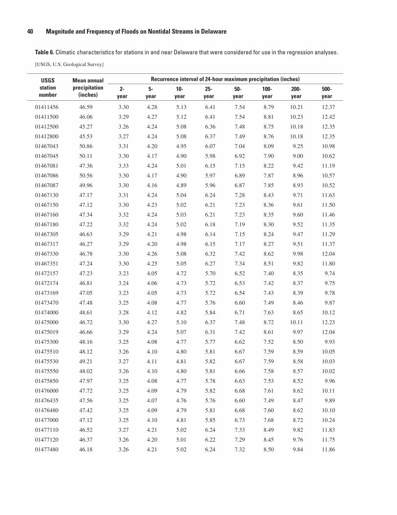
Table �. Climatic characteristics for stations in and near Delaware that were considered for use in the regression analyses.
[USGS, U.S. Geological Survey]
USGS station number
Mean annual precipitation
(inches)
Recurrence interval of ��-hour maximum precipitation (inches)
�- year
�- year
10- year
��- year
�0- year
100- year
�00- year
�00- year
01411456 46.59 3.30 4.28 5.13 6.41 7.54 8.79 10.21 12.37
01411500 46.06 3.29 4.27 5.12 6.41 7.54 8.81 10.23 12.42
01412500 45.27 3.26 4.24 5.08 6.36 7.48 8.75 10.18 12.35
01412800 45.53 3.27 4.24 5.08 6.37 7.49 8.76 10.18 12.35
01467043 50.86 3.31 4.20 4.95 6.07 7.04 8.09 9.25 10.98
01467045 50.11 3.30 4.17 4.90 5.98 6.92 7.90 9.00 10.62
01467081 47.36 3.33 4.24 5.01 6.15 7.15 8.22 9.42 11.19
01467086 50.56 3.30 4.17 4.90 5.97 6.89 7.87 8.96 10.57
01467087 49.96 3.30 4.16 4.89 5.96 6.87 7.85 8.93 10.52
01467130 47.17 3.31 4.24 5.04 6.24 7.28 8.43 9.71 11.63
01467150 47.12 3.30 4.23 5.02 6.21 7.23 8.36 9.61 11.50
01467160 47.34 3.32 4.24 5.03 6.21 7.23 8.35 9.60 11.46
01467180 47.22 3.32 4.24 5.02 6.18 7.19 8.30 9.52 11.35
01467305 46.63 3.29 4.21 4.98 6.14 7.15 8.24 9.47 11.29
01467317 46.27 3.29 4.20 4.98 6.15 7.17 8.27 9.51 11.37
01467330 46.78 3.30 4.26 5.08 6.32 7.42 8.62 9.98 12.04
01467351 47.24 3.30 4.25 5.05 6.27 7.34 8.51 9.82 11.80
01472157 47.23 3.23 4.05 4.72 5.70 6.52 7.40 8.35 9.74
01472174 46.81 3.24 4.06 4.73 5.72 6.53 7.42 8.37 9.75
01473169 47.05 3.23 4.05 4.73 5.72 6.54 7.43 8.39 9.78
01473470 47.48 3.25 4.08 4.77 5.76 6.60 7.49 8.46 9.87
01474000 48.61 3.28 4.12 4.82 5.84 6.71 7.63 8.65 10.12
01475000 46.72 3.30 4.27 5.10 6.37 7.48 8.72 10.11 12.23
01475019 46.66 3.29 4.24 5.07 6.31 7.42 8.61 9.97 12.04
01475300 48.16 3.25 4.08 4.77 5.77 6.62 7.52 8.50 9.93
01475510 48.12 3.26 4.10 4.80 5.81 6.67 7.59 8.59 10.05
01475530 49.21 3.27 4.11 4.81 5.82 6.67 7.59 8.58 10.03
01475550 48.02 3.26 4.10 4.80 5.81 6.66 7.58 8.57 10.02
01475850 47.97 3.25 4.08 4.77 5.78 6.63 7.53 8.52 9.96
01476000 47.72 3.25 4.09 4.79 5.82 6.68 7.61 8.62 10.11
01476435 47.56 3.25 4.07 4.76 5.76 6.60 7.49 8.47 9.89
01476480 47.42 3.25 4.09 4.79 5.81 6.68 7.60 8.62 10.10
01477000 47.12 3.25 4.10 4.81 5.85 6.73 7.68 8.72 10.24
01477110 46.52 3.27 4.21 5.02 6.24 7.33 8.49 9.82 11.83
01477120 46.37 3.26 4.20 5.01 6.22 7.29 8.45 9.76 11.75
01477480 46.18 3.26 4.21 5.02 6.24 7.32 8.50 9.84 11.86
�0 Magnitude and Frequency of Floods on Nontidal Streams in Delaware

Table �. Climatic characteristics for stations in and near Delaware that were considered for use in the regression analyses.—Continued
[USGS, U.S. Geological Survey]
USGS station number
Mean annual precipitation
(inches)
Recurrence interval of ��-hour maximum precipitation (inches)
�- year
�- year
10- year
��- year
�0- year
100- year
�00- year
�00- year
01477500 46.07 3.26 4.21 5.02 6.24 7.31 8.50 9.83 11.84
01477800 46.77 3.27 4.13 4.84 5.89 6.77 7.73 8.77 10.30
01478000 45.86 3.25 4.07 4.77 5.78 6.62 7.53 8.52 9.96
01478040 45.08 3.24 4.08 4.78 5.80 6.67 7.59 8.61 10.08
01478200 47.83 3.25 4.08 4.77 5.76 6.60 7.50 8.47 9.88
01478500 47.39 3.26 4.08 4.77 5.77 6.61 7.51 8.48 9.89
01479000 46.97 3.26 4.08 4.77 5.78 6.62 7.52 8.49 9.91
01479200 48.07 3.27 4.10 4.79 5.80 6.64 7.55 8.53 9.96
01479820 47.68 3.27 4.10 4.79 5.79 6.63 7.53 8.50 9.91
01479950 47.47 3.27 4.11 4.80 5.81 6.66 7.57 8.56 9.99
01480000 47.69 3.27 4.10 4.80 5.80 6.64 7.55 8.52 9.94
01480015 47.53 3.27 4.10 4.80 5.80 6.65 7.55 8.53 9.95
01480100 45.84 3.27 4.12 4.81 5.83 6.68 7.60 8.60 10.05
01480300 47.81 3.21 4.02 4.70 5.68 6.49 7.37 8.32 9.70
01480500 47.76 3.22 4.03 4.71 5.69 6.51 7.39 8.34 9.72
01480610 47.25 3.24 4.05 4.73 5.72 6.54 7.43 8.38 9.77
01480675 47.58 3.24 4.06 4.74 5.72 6.54 7.42 8.38 9.77
01480680 47.29 3.24 4.06 4.74 5.72 6.54 7.43 8.38 9.77
01480700 47.24 3.24 4.05 4.73 5.71 6.53 7.42 8.37 9.75
01480870 47.11 3.24 4.06 4.74 5.72 6.54 7.42 8.38 9.76
01481000 47.25 3.25 4.07 4.75 5.74 6.56 7.45 8.41 9.80
01481200 47.94 3.28 4.12 4.82 5.83 6.68 7.60 8.59 10.02
01481450 47.62 3.28 4.13 4.84 5.87 6.73 7.67 8.70 10.18
01481500 47.29 3.25 4.07 4.75 5.74 6.57 7.46 8.43 9.83
01482310 43.93 3.22 4.10 4.83 5.92 6.88 7.88 9.01 10.68
01482500 46.06 3.26 4.22 5.04 6.29 7.39 8.60 9.97 12.05
01483000 45.48 3.26 4.23 5.06 6.32 7.42 8.65 10.05 12.16
01483200 44.41 3.20 4.14 4.94 6.17 7.24 8.43 9.77 11.81
01483290 44.55 3.21 4.15 4.96 6.19 7.27 8.47 9.82 11.88
01483400 44.34 3.20 4.14 4.95 6.18 7.25 8.45 9.80 11.85
01483500 44.51 3.25 4.22 5.05 6.32 7.43 8.67 10.07 12.21
01483700 44.62 3.27 4.25 5.10 6.39 7.53 8.79 10.23 12.42
01483720 44.56 3.30 4.29 5.14 6.45 7.60 8.88 10.35 12.57
01484000 44.86 3.31 4.30 5.16 6.47 7.63 8.92 10.38 12.60
01484002 44.83 3.33 4.33 5.20 6.52 7.68 8.98 10.46 12.70
01484050 44.80 3.33 4.33 5.19 6.51 7.67 8.97 10.44 12.69
01484100 44.94 3.35 4.36 5.23 6.56 7.73 9.04 10.51 12.77
01484270 45.37 3.41 4.43 5.32 6.67 7.86 9.19 10.70 13.00
Tables � through � �1

Table �. Climatic characteristics for stations in and near Delaware that were considered for use in the regression analyses.—Continued
[USGS, U.S. Geological Survey]
USGS station number
Mean annual precipitation
(inches)
Recurrence interval of ��-hour maximum precipitation (inches)
�- year
�- year
10- year
��- year
�0- year
100- year
�00- year
�00- year
01477500 46.07 3.26 4.21 5.02 6.24 7.31 8.50 9.83 11.84
01477800 46.77 3.27 4.13 4.84 5.89 6.77 7.73 8.77 10.30
01478000 45.86 3.25 4.07 4.77 5.78 6.62 7.53 8.52 9.96
01478040 45.08 3.24 4.08 4.78 5.80 6.67 7.59 8.61 10.08
01478200 47.83 3.25 4.08 4.77 5.76 6.60 7.50 8.47 9.88
01478500 47.39 3.26 4.08 4.77 5.77 6.61 7.51 8.48 9.89
01479000 46.97 3.26 4.08 4.77 5.78 6.62 7.52 8.49 9.91
01479200 48.07 3.27 4.10 4.79 5.80 6.64 7.55 8.53 9.96
01479820 47.68 3.27 4.10 4.79 5.79 6.63 7.53 8.50 9.91
01479950 47.47 3.27 4.11 4.80 5.81 6.66 7.57 8.56 9.99
01480000 47.69 3.27 4.10 4.80 5.80 6.64 7.55 8.52 9.94
01480015 47.53 3.27 4.10 4.80 5.80 6.65 7.55 8.53 9.95
01480100 45.84 3.27 4.12 4.81 5.83 6.68 7.60 8.60 10.05
01480300 47.81 3.21 4.02 4.70 5.68 6.49 7.37 8.32 9.70
01480500 47.76 3.22 4.03 4.71 5.69 6.51 7.39 8.34 9.72
01480610 47.25 3.24 4.05 4.73 5.72 6.54 7.43 8.38 9.77
01480675 47.58 3.24 4.06 4.74 5.72 6.54 7.42 8.38 9.77
01480680 47.29 3.24 4.06 4.74 5.72 6.54 7.43 8.38 9.77
01480700 47.24 3.24 4.05 4.73 5.71 6.53 7.42 8.37 9.75
01480870 47.11 3.24 4.06 4.74 5.72 6.54 7.42 8.38 9.76
01481000 47.25 3.25 4.07 4.75 5.74 6.56 7.45 8.41 9.80
01481200 47.94 3.28 4.12 4.82 5.83 6.68 7.60 8.59 10.02
01481450 47.62 3.28 4.13 4.84 5.87 6.73 7.67 8.70 10.18
01481500 47.29 3.25 4.07 4.75 5.74 6.57 7.46 8.43 9.83
01482310 43.93 3.22 4.10 4.83 5.92 6.88 7.88 9.01 10.68
01482500 46.06 3.26 4.22 5.04 6.29 7.39 8.60 9.97 12.05
01483000 45.48 3.26 4.23 5.06 6.32 7.42 8.65 10.05 12.16
01483200 44.41 3.20 4.14 4.94 6.17 7.24 8.43 9.77 11.81
01483290 44.55 3.21 4.15 4.96 6.19 7.27 8.47 9.82 11.88
01483400 44.34 3.20 4.14 4.95 6.18 7.25 8.45 9.80 11.85
01483500 44.51 3.25 4.22 5.05 6.32 7.43 8.67 10.07 12.21
01483700 44.62 3.27 4.25 5.10 6.39 7.53 8.79 10.23 12.42
01483720 44.56 3.30 4.29 5.14 6.45 7.60 8.88 10.35 12.57
01484000 44.86 3.31 4.30 5.16 6.47 7.63 8.92 10.38 12.60
01484002 44.83 3.33 4.33 5.20 6.52 7.68 8.98 10.46 12.70
01484050 44.80 3.33 4.33 5.19 6.51 7.67 8.97 10.44 12.69
01484100 44.94 3.35 4.36 5.23 6.56 7.73 9.04 10.51 12.77
01484270 45.37 3.41 4.43 5.32 6.67 7.86 9.19 10.70 13.00
01484300 45.11 3.39 4.40 5.29 6.62 7.80 9.12 10.62 12.90
�� Magnitude and Frequency of Floods on Nontidal Streams in Delaware

Table �. Climatic characteristics for stations in and near Delaware that were considered for use in the regression analyses.—Continued
[USGS, U.S. Geological Survey]
USGS station number
Mean annual precipitation
(inches)
Recurrence interval of ��-hour maximum precipitation (inches)
�- year
�- year
10- year
��- year
�0- year
100- year
�00- year
�00- year
01484500 45.61 3.42 4.45 5.34 6.69 7.88 9.22 10.73 13.03
01484525 45.52 3.42 4.45 5.34 6.69 7.88 9.22 10.73 13.03
01484550 45.65 3.42 4.44 5.33 6.68 7.86 9.20 10.71 13.00
01485000 45.49 3.44 4.47 5.37 6.73 7.93 9.27 10.79 13.11
01485500 45.33 3.47 4.51 5.41 6.79 7.99 9.35 10.89 13.22
01486000 44.90 3.35 4.35 5.22 6.54 7.71 9.02 10.49 12.74
01486100 45.38 3.45 4.49 5.39 6.75 7.95 9.30 10.82 13.15
01486980 44.98 3.36 4.37 5.25 6.58 7.76 9.07 10.55 12.81
01487000 44.98 3.36 4.37 5.25 6.58 7.75 9.06 10.54 12.80
01487500 45.35 3.44 4.47 5.36 6.72 7.91 9.25 10.77 13.08
01488000 44.67 3.42 4.45 5.34 6.69 7.88 9.22 10.73 13.03
Tables � through � ��

Table �. Basin characteristics for stations in and near Delaware that were considered for use in the regression analyses.
[USGS, U.S. Geological Survey; mi2, square miles; ft/mi, NHD, National Hydrography Dataset; NLCD.DE, 2001 National Land Cover Dataset and 2003 Delaware land cover dataset combined; feet per mile; mi, miles; in/hr, inches per hour; ft, feet]
USGS station number
Drain- age area (mi�)
Mean stream slope (ft/mi)
10/�� stream slope (ft/mi)
Mean basin slope
(percent)
Storage (NHD)
(percent)
Storage (NLCD.DE) (percent)
Forest cover
(percent)
Main channel length
(mi)
Basin shape factor
Hydro- logic soil
type A (percent)
01411456 9.78 8.84 8.07 0.72 12.3 18.8 59.9 5.40 2.98 12.501411500 112 6.16 4.84 0.99 9.27 11.7 50.8 19.7 3.46 13.601412500 2.55 25.0 22.6 2.09 0.06 1.39 4.87 3.36 4.43 0.5301412800 28.0 11.6 11.2 1.93 1.27 4.53 16.3 8.58 2.63 4.5501467043 1.20 71.8 67.1 4.39 0.00 0.57 13.4 2.13 3.80 6.25
01467045 43.1 20.4 16.7 4.75 0.47 0.96 19.1 14.7 5.02 2.8201467081 8.98 12.2 9.72 1.88 0.31 5.81 17.3 8.64 8.31 5.3901467086 16.2 38.3 26.9 5.23 0.33 1.49 13.5 9.40 5.46 5.9801467087 30.0 31.8 21.8 4.41 0.36 1.29 9.43 12.9 5.57 6.3101467089 33.8 30.9 20.8 4.11 0.33 1.20 8.44 13.8 5.59 6.56
01467130 5.03 32.5 20.0 2.71 2.47 11.2 44.2 4.11 3.36 30.001467150 17.1 18.3 11.2 2.69 1.25 7.58 29.9 9.92 5.75 11.701467160 5.32 24.0 12.8 2.57 0.34 8.22 29.8 6.16 7.13 3.2201467180 10.5 18.9 11.1 2.64 0.33 9.55 32.1 9.18 8.01 3.6401467305 1.33 41.8 30.3 1.21 0.31 3.49 21.1 2.31 4.04 6.00
01467317 0.62 43.5 45.5 1.51 0.28 2.38 11.0 1.46 3.44 6.0001467330 20.8 20.6 20.4 3.19 3.80 7.91 31.2 8.44 3.42 5.1701467351 7.16 24.8 27.3 3.69 2.66 6.81 36.7 5.63 4.43 35.301472157 59.0 36.1 25.1 9.53 0.73 2.44 53.1 19.0 6.08 5.4301472174 5.98 73.4 38.6 8.00 0.48 2.01 30.7 4.74 3.77 6.25
01473169 20.8 47.3 29.7 8.72 0.37 3.60 29.8 9.93 4.73 1.9701473470 20.8 35.6 28.1 4.39 0.24 0.24 16.3 7.87 2.97 0.0001474000 63.7 64.3 13.3 5.45 0.57 1.17 24.0 25.4 10.1 1.2601475000 6.05 17.7 19.2 2.07 2.58 5.23 19.2 4.50 3.35 4.0301475019 14.1 17.3 17.9 2.59 2.42 5.87 23.4 8.02 4.56 2.66
01475300 5.18 56.2 36.8 5.59 0.36 1.01 30.5 4.08 3.21 3.4701475510 37.6 28.2 21.0 6.90 0.46 1.00 24.7 18.3 8.94 6.2101475530 4.78 63.7 61.7 4.42 0.15 1.26 11.2 4.71 4.64 6.4601475550 21.8 35.4 32.2 4.08 0.27 1.17 8.17 11.8 6.34 7.3601475850 15.8 43.6 32.0 6.56 0.43 1.74 36.8 8.67 4.75 1.95
01476000 33.7 27.6 22.0 7.77 2.30 3.92 35.1 20.1 12.0 3.2501476435 9.71 40.8 32.7 5.54 0.56 1.31 24.9 6.42 4.24 3.1601476480 30.2 29.3 23.4 7.79 0.58 0.93 41.1 16.8 9.35 1.7401476500 31.6 28.4 22.3 7.88 0.59 0.96 40.8 18.2 10.4 1.9401477000 60.7 27.9 22.7 7.67 0.92 1.80 32.2 20.9 7.19 3.35
01477110 14.6 14.4 15.1 2.65 2.17 5.42 29.6 8.17 4.57 7.3201477120 25.9 13.4 14.8 2.84 1.77 5.70 29.5 10.3 4.10 5.19
�� Magnitude and Frequency of Floods on Nontidal Streams in Delaware

Table �. Basin characteristics for stations in and near Delaware that were considered for use in the regression analyses.— Continued
[USGS, U.S. Geological Survey; mi2, square miles; ft/mi, NHD, National Hydrography Dataset; NLCD.DE, 2001 National Land Cover Dataset and 2003 Delaware land cover dataset combined; feet per mile; mi, miles; in/hr, inches per hour; ft, feet]
Hydro- logic soil
type D (percent)
Average soil
permea- bility (in/hr)
Imper- vious area
(percent)
Basin relief
(ft)
Mean basin eleva tion (ft)
Gage elevation
(ft)
Develop- ment
intensity (percent)
Devel- oped area
(percent)
Centroid year
housing density (homes/
acre)
�000 Housing density (homes/
acre)
USGS station number
8.09 6.91 4.22 48.6 134 112 4.25 15.8 0.26 0.28 014114567.08 6.86 3.27 131 115 48.7 3.21 13.9 0.15 0.26 014115000.00 1.83 0.13 93.3 105 47.9 0.06 0.46 0.06 0.07 014125000.74 2.84 0.80 114 103 27.4 0.76 2.87 0.07 0.08 014128007.29 1.23 25.8 154 207 96.9 22.5 80.6 2.92 2.99 01467043
5.67 1.12 20.3 364 251 69.2 19.7 69.4 1.56 1.99 014670450.53 2.67 31.0 106 63.1 17.0 29.1 77.6 1.80 1.98 014670816.97 1.23 24.6 366 254 63.8 23.7 79.2 3.80 3.94 014670867.69 1.23 38.3 417 220 18.3 37.3 85.6 6.70 6.74 014670878.32 1.23 41.1 430 206 3.28 40.0 87.0 7.16 7.25 01467089
4.47 6.99 14.2 145 104 56.5 13.2 41.6 0.52 0.97 014671302.68 3.82 19.4 193 84.9 5.80 18.4 60.7 1.22 1.39 014671503.37 2.61 16.7 157 91.6 33.7 15.2 59.5 0.35 1.38 014671602.26 2.52 17.6 183 78.0 8.92 16.6 60.6 0.57 1.35 014671800.00 2.64 18.2 103 70.2 18.9 17.4 78.1 3.42 3.47 01467305
0.00 2.64 23.8 64.8 73.4 37.9 22.7 89.0 3.28 3.28 014673172.53 3.96 14.4 180 112 9.15 13.4 47.0 0.62 1.12 014673305.25 7.83 15.5 182 114 19.1 14.5 50.2 1.92 1.94 014673517.00 1.65 0.45 838 529 167 0.44 2.03 0.08 0.10 014721577.29 1.23 3.70 355 437 277 3.33 14.0 0.06 0.24 01472174
2.33 1.24 12.7 635 354 117 12.5 38.6 0.58 0.66 014731698.07 1.06 15.8 412 283 78.8 14.8 52.3 1.02 1.29 014734706.89 1.07 13.8 469 283 20.6 13.6 54.7 1.53 1.68 014740002.58 4.20 14.6 90.1 128 69.6 13.4 49.0 0.45 1.67 014750002.79 3.64 13.8 150 105 11.7 12.7 46.6 0.68 1.25 01475019
12.0 0.95 8.25 245 434 316 9.01 42.3 0.78 0.93 0147530010.7 1.15 15.7 531 325 28.3 15.0 56.9 1.90 2.03 01475510
7.85 1.23 22.6 311 319 126 21.5 81.4 3.19 3.33 0147553010.3 1.23 37.5 426 209 17.1 36.0 87.6 6.84 6.89 0147555014.6 0.79 3.56 382 419 218 4.10 20.6 0.49 0.53 01475850
13.6 0.90 7.24 561 336 35.4 7.30 32.3 0.47 0.82 0147600012.6 0.91 5.48 270 472 342 5.51 28.9 0.40 0.83 0147643515.0 0.77 3.83 499 373 110 3.82 19.5 0.20 0.57 0147648014.7 0.79 4.42 523 367 87.3 4.42 20.8 0.21 0.66 0147650012.3 0.93 7.74 586 338 24.6 7.78 29.8 0.30 0.62 01477000
5.35 4.98 1.60 140 115 31.0 1.60 8.13 0.12 0.15 014771103.86 3.93 1.67 163 102 10.6 1.56 7.78 0.11 0.14 01477120
Tables � through � ��

Table �. Basin characteristics for stations in and near Delaware that were considered for use in the regression analyses.— Continued
[USGS, U.S. Geological Survey; mi2, square miles; ft/mi, NHD, National Hydrography Dataset; NLCD.DE, 2001 National Land Cover Dataset and 2003 Delaware land cover dataset combined; feet per mile; mi, miles; in/hr, inches per hour; ft, feet]
USGS station number
Drain-age area (mi�)
Mean stream slope (ft/mi)
10/�� stream slope (ft/mi)
Mean basin slope
(percent)
Storage (NHD)
(percent)
Storage (NLCD.DE) (percent)
Forest cover
(percent)
Main channel length
(mi)
Basin shape factor
Hydro-logic soil
type A (percent)
01477480 13.8 14.5 13.5 2.47 1.31 5.33 31.8 9.16 6.09 5.4501477500 18.5 13.7 13.5 2.67 0.99 5.31 28.8 9.87 5.26 6.4401477800 7.34 65.3 65.4 3.70 0.13 0.23 7.29 6.10 5.07 1.56
01478000 20.8 30.5 21.7 4.71 0.43 2.26 23.7 13.4 8.67 2.6101478040 40.6 23.2 17.6 3.38 1.06 4.71 25.1 18.1 8.08 1.3301478200 12.7 36.8 27.5 6.63 0.18 0.66 15.9 11.0 9.53 6.2301478500 66.4 25.2 17.7 8.16 0.36 1.54 25.7 19.5 5.70 5.9001478650 68.6 23.3 16.7 8.22 0.41 1.59 26.5 21.7 6.86 5.82
01479000 88.9 20.0 13.9 7.69 0.42 1.56 25.1 27.2 8.32 5.1201479200 4.29 60.1 42.8 6.39 0.33 0.76 10.7 3.38 2.67 6.2501479820 27.6 32.8 20.9 6.90 0.64 1.76 19.6 10.8 4.22 5.8401479950 0.38 173 149 14.7 0.00 0.00 35.2 1.40 5.14 6.2501480000 47.2 23.8 15.9 8.58 1.36 2.07 25.1 19.3 7.88 6.01
01480015 52.5 22.3 15.4 8.34 1.31 2.03 23.8 23.7 10.7 5.8801480100 6.67 46.2 33.4 4.08 0.35 0.53 13.8 6.55 6.44 7.2201480300 18.7 44.9 24.4 5.23 0.26 3.15 22.0 9.22 4.56 5.3601480500 46.1 33.6 22.0 6.75 0.69 3.27 34.3 20.7 9.31 2.4201480610 2.61 124 145 9.96 0.23 4.74 31.8 2.65 2.68 3.74
01480617 55.3 31.1 21.5 7.48 0.67 3.83 33.9 23.7 10.1 2.6401480675 8.54 41.3 26.9 7.11 6.04 5.46 46.3 6.01 4.23 6.2501480680 17.6 39.9 31.6 7.80 5.15 5.57 39.1 9.13 4.72 6.2501480700 60.1 43.8 23.5 7.49 2.92 4.62 37.5 17.9 5.30 5.9901480800 81.8 40.3 22.0 7.61 2.26 4.22 35.5 20.2 4.97 5.39
01480870 89.8 35.0 19.9 7.95 2.14 4.27 36.2 24.1 6.46 5.3601481000 288 19.4 13.8 8.53 1.15 3.28 31.5 43.6 6.59 4.6501481200 1.05* 142 134 15.2 0.19 0.26 48.2 1.93 3.53 6.2501481450 0.31* 72.1 74.7 3.11 0.00 0.00 4.07 0.92 2.69 0.0001481500 319 17.2 11.2 8.63 1.21 3.26 31.8 54.4 9.28 4.59
01482310 1.05 32.1 32.0 2.22 0.82 4.92 13.3 1.81 3.10 0.0001482500 14.6 15.0 11.7 2.55 1.71 4.13 17.9 8.11 4.51 3.8801483000 20.4 13.8 13.6 2.86 2.83 5.29 39.0 9.35 4.29 11.601483200 4.06* 14.4 14.8 1.76 4.39 17.7 30.7 4.19 4.33 3.0701483290 1.2* 11.9 11.7 1.16 1.67 10.4 7.34 2.40 4.79 3.06
01483400 0.51* 30.3 28.2 1.70 2.59 18.0 7.44 1.08 2.3 3.0601483500 9.15 9.04 8.22 1.46 0.89 11.3 9.40 5.86 3.75 3.601483700 31.0 4.87 4.95 1.06 4.28 16.1 14.0 13.7 6.04 3.7101483720 2.54* 14.0 14.3 1.01 0.06 3.33 9.95 2.53 2.51 3.06
�� Magnitude and Frequency of Floods on Nontidal Streams in Delaware

Table �. Basin characteristics for stations in and near Delaware that were considered for use in the regression analyses— Continued.
[USGS, U.S. Geological Survey; mi2, square miles; ft/mi, NHD, National Hydrography Dataset; NLCD.DE, 2001 National Land Cover Dataset
and 2003 Delaware land cover dataset combined; feet per mile; mi, miles; in/hr, inches per hour; ft, feet]
Hydro-logic soil
type D (percent)
Average soil
permea-bility (in/hr)
Imper-vious area
(percent)
Basin relief
(ft)
Mean basin eleva-
tion (ft)
Gage elevation
(ft)
Develop-ment
intensity (percent)
Devel-oped area
(percent)
Centroid year
housing density (homes/
acre)
�000 Housing density (homes/
acre)
USGS station number
23.8 4.06 0.33 148 109 17.2 0.34 1.76 0.05 0.05 0147748019.4 4.34 0.31 150 105 13.0 0.31 1.57 0.02 0.05 0147750019.1 0.66 18.6 400 275 21.9 31.5 90.7 1.74 1.87 01477800
7.98 1.25 11.0 412 191 28.6 16.3 40.0 0.50 0.74 014780006.61 1.38 11.6 423 135 17.0 20.5 47.4 0.59 0.80 014780407.27 1.23 1.03 414 452 235 1.09 6.18 0.10 0.16 014782006.88 1.23 1.64 582 376 70.4 2.19 9.79 0.12 0.20 014785006.92 1.23 1.84 597 369 55.5 2.54 10.7 0.21 0.21 01478650
7.19 1.23 5.10 636 324 16.2 8.06 23.1 0.15 0.50 014790007.29 1.23 8.22 226 313 214 23.7 76.8 0.20 0.72 014792006.81 1.23 3.75 361 370 190 3.83 15.8 0.30 0.31 014798207.29 1.23 0.56 269 305 147 8.94 37.8 0.15 0.42 014799507.01 1.23 2.55 467 336 84.7 5.82 24.8 0.18 0.29 01480000
7.08 1.23 3.90 536 320 15.7 8.09 30.7 0.37 0.38 0148001514.2 1.13 22.6 304 155 49.7 34.1 83.0 1.64 1.67 01480100
6.3 1.47 1.35 463 726 590 1.24 4.33 0.10 0.15 0148030011.5 1.10 1.47 743 663 306 1.31 5.95 0.09 0.20 01480500
5.86 1.17 4.38 331 543 354 4.17 20.7 0.33 0.38 01480610
10.5 1.12 3.82 783 632 266 3.56 11.3 0.30 0.35 014806177.29 1.23 0.60 381 598 452 0.57 2.79 0.06 0.08 014806757.29 1.23 1.33 494 557 336 1.21 6.53 0.03 0.12 014806806.98 1.31 1.66 795 558 261 1.48 6.42 0.12 0.19 014807006.53 1.32 3.08 826 531 228 2.82 11.6 0.07 0.32 01480800
6.48 1.31 3.71 855 516 199 3.47 13.2 0.27 0.35 014808707.79 1.21 3.38 901 489 154 3.23 12.4 0.11 0.34 014810007.29 1.23 0.40 282 327 157 8.57 34.5 0.07 0.11 01481200
18.0 0.59 23.7 70.7 355 312 34.8 95.9 1.51 1.51 014814508.11 1.19 3.45 987 472 67.3 3.91 14.4 0.19 0.34 01481500
2.15 1.76 5.57 58.8 58.1 21.4 13.8 25.7 0.08 0.21 014823104.47 3.03 0.89 133 110 31.0 0.99 4.34 0.04 0.06 014825003.79 3.29 0.13 151 82.2 10.1 0.14 0.92 0.03 0.04 014830003.05 2.87 0.05 63.1 62.8 19.8 2.25 9.91 0.03 0.04 014832003.06 2.87 0.14 34.6 64.0 45.6 2.99 13.4 0.02 0.06 01483290
3.06 2.87 0.94 33.8 52.9 36.2 13.6 29.1 0.02 0.06 014834003.06 2.98 0.56 56.1 58.7 20.0 3.31 14.9 0.02 0.07 014835002.70 2.78 5.30 67.7 51.4 12.6 11.0 31.4 0.22 0.31 014837003.06 2.87 12.4 36.0 45.3 24.1 22.2 36.6 0.33 0.64 01483720
Tables � through � ��
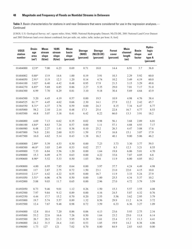
Table �. Basin characteristics for stations in and near Delaware that were considered for use in the regression analyses.— Continued
[USGS, U.S. Geological Survey; mi2, square miles; ft/mi, NHD, National Hydrography Dataset; NLCD.DE, 2001 National Land Cover Dataset
and 2003 Delaware land cover dataset combined; feet per mile; mi, miles; in/hr, inches per hour; ft, feet]
USGS station number
Drain- age area (mi�)
Mean stream slope (ft/mi)
10/�� stream slope (ft/mi)
Mean basin slope
(percent)
Storage (NHD)
(percent)
Storage (NLCD.DE) (percent)
Forest cover
(percent)
Main channel length
(mi)
Basin shape factor
Hydro- logic soil
type A (percent)
01484000 12.9* 7.00 6.23 0.69 0.71 18.0 14.4 6.91 3.7 36.8
01484002 0.88* 13.9 14.6 1.00 0.19 3.91 10.3 2.29 5.92 60.001484050 2.91* 11.9 12.3 1.20 0.14 4.74 10.2 3.49 4.19 60.001484100 3.02* 6.40 4.42 0.48 0.95 17.9 21.5 3.15 3.29 49.801484270 6.85* 5.69 6.85 0.86 2.27 5.35 29.0 7.01 7.17 51.001484300 6.99 7.70 8.29 0.81 3.10 9.18 30.4 5.69 4.64 43.9
01484500 5.20 4.45 4.19 0.57 0.00 19.5 10.9 4.98 4.76 38.401484525 61.7* 4.45 4.62 0.66 2.30 14.1 27.9 12.2 2.42 45.701484550 8.31* 4.37 3.76 0.59 0.00 24.3 8.15 7.34 6.47 6.7701485000 58.2 2.10 2.14 0.48 17.3 25.4 22.8 16.7 4.77 8.5301485500 44.8 5.07 3.18 0.41 6.42 8.22 66.0 13.3 3.91 18.2
01486000 4.69 7.13 6.62 0.35 0.02 9.98 56.1 3.68 2.89 6.0101486100 4.84* 8.63 7.24 0.57 0.00 1.11 57.1 4.88 4.93 7.1701486980 6.48 2.27 1.41 0.36 0.10 25.2 26.3 4.47 3.08 17.601487000 74.0 2.81 2.60 0.53 1.59 17.9 16.8 15.1 3.07 17.901487500 16.0 4.62 5.14 0.43 1.38 16.2 40.1 9.00 5.06 46.2
01488000 2.89* 5.39 4.53 0.30 0.00 7.23 3.73 3.30 3.77 59.501488500 46.8* 3.03 2.49 0.53 0.02 27.7 8.3 12.3 3.21 8.5501489000 7.33 6.84 5.56 1.20 0.00 1.64 19.8 6.06 5.01 4.7001490000 15.3 6.09 4.75 0.63 0.00 4.22 33.6 7.87 4.05 6.801490600 8.90* 5.52 5.33 0.50 1.03 36.6 11.9 6.00 4.05 10.2
01490800 4.00 6.95 7.85 0.64 0.00 3.97 37.7 4.24 4.49 4.9801491000 117 2.87 2.75 0.72 1.50 23.1 21.0 22.0 4.15 10.001491010 2.11* 4.42 4.22 0.55 0.00 16.7 11.9 3.33 5.24 27.901491050 3.51* 6.06 4.76 0.50 0.00 1.00 25.5 4.34 5.37 10.201492000 5.88 9.03 11.7 0.65 0.00 2.96 27.0 4.72 3.79 3.59
01492050 8.73 9.46 9.01 1.12 0.26 1.50 15.3 5.57 3.55 4.0801492500 7.97 9.84 9.12 0.89 0.00 4.16 24.5 5.87 4.32 0.7601492550 4.44 17.7 15.2 0.70 0.20 2.55 5.56 3.62 2.95 3.7901493000 19.7 5.74 5.57 0.89 1.32 8.56 29.9 11.2 6.34 3.7201493500 12.4 7.67 9.48 0.98 0.72 3.59 6.33 6.36 3.27 1.09
01494000 12.8 10.4 7.20 0.86 0.06 4.13 23.6 5.93 2.75 2.3401495000 53.2 22.8 16.6 7.26 0.50 1.64 23.2 25.0 11.8 6.1401495500 26.7 28.5 23.3 5.95 0.39 1.61 23.4 17.3 11.3 4.4101496000 24.2 31.5 24.4 3.83 0.53 1.85 19.9 14.2 8.38 4.0601496080 1.73 127 121 7.02 0.70 8.80 84.9 2.83 4.63 0.00
�� Magnitude and Frequency of Floods on Nontidal Streams in Delaware

Table �. Basin characteristics for stations in and near Delaware that were considered for use in the regression analyses.— Continued
[USGS, U.S. Geological Survey; mi2, square miles; ft/mi, NHD, National Hydrography Dataset; NLCD.DE, 2001 National Land Cover Dataset
and 2003 Delaware land cover dataset combined; feet per mile; mi, miles; in/hr, inches per hour; ft, feet]
Hydro- logic soil
type D (percent)
Average soil
permea- bility (in/hr)
Imper- vious area
(percent)
Basin relief
(ft)
Mean basin eleva-
tion (ft)
Gage eleva-
tion (ft)
Develop- ment
intensity (percent)
Devel- oped area
(percent)
Centroid year
housing density (homes/
acre)
�000 Housing density (homes/
acre)
USGS station number
4.31 2.92 0.84 52.0 55.0 21.3 3.68 13.5 0.04 0.09 01484000
6.00 3.15 0.69 32.6 54.3 28.1 1.40 2.19 0.03 0.08 014840025.99 3.15 2.01 48.5 52.8 22.9 7.40 22.6 0.02 0.08 014840505.25 3.05 0.01 25.8 53.1 37.5 1.49 6.33 0.03 0.06 014841004.91 2.90 0.72 51.2 34.5 4.19 4.08 13.3 0.05 0.08 014842704.76 3.37 0.50 45.8 37.1 8.33 1.99 7.55 0.02 0.05 01484300
3.05 2.60 2.62 29.4 43.8 26.8 8.17 19.0 0.03 0.07 014845004.29 2.95 1.48 62.0 39.7 1.00 5.58 15.4 0.08 0.09 01484525
10.1 3.93 1.34 35.9 33.7 9.08 3.76 11.9 0.03 0.05 0148455013.0 4.00 0.16 55.8 41.1 19.2 0.87 3.63 0.02 0.03 01485000
6.09 4.49 0.12 74.8 44.3 14.3 0.12 0.66 0.02 0.04 01485500
2.00 3.22 0.12 35.3 28.6 17.5 0.10 0.62 0.01 0.02 014860001.35 2.15 0.03 40.3 59.3 39.2 0.03 0.13 0.01 0.06 014861002.91 2.74 0.38 39.6 51.9 44.1 2.96 11.0 0.01 0.03 014869803.49 3.04 0.87 65.6 48.6 18.8 3.35 11.2 0.02 0.04 014870004.89 3.21 0.05 49.4 48.7 28.8 1.22 5.12 0.02 0.03 01487500
5.96 3.16 0.01 17.9 37.0 28.6 2.10 8.93 0.01 0.04 014880002.45 2.93 0.12 38.9 55.8 31.2 1.37 6.23 0.02 0.04 014885002.58 2.91 0.14 42.6 44.4 17.5 0.11 0.53 0.02 0.04 014890003.19 3.57 0.11 49.1 29.2 2.72 0.11 0.36 0.02 0.02 014900002.87 3.15 0.04 34.1 58.1 36.6 1.56 7.03 0.01 0.04 01490600
2.02 2.62 0.86 29.9 57.2 35.7 0.80 3.13 0.02 0.04 014908002.80 3.10 0.28 103 57.1 11.4 2.24 9.60 0.03 0.06 014910004.94 4.68 0.03 18.0 58.5 46.7 0.28 2.11 0.01 0.02 014910102.66 3.08 0.10 26.3 56.5 39.2 0.12 0.68 0.02 0.06 014910502.28 2.34 0.18 43.2 52.3 16.9 0.21 1.26 0.01 0.03 01492000
3.82 3.55 0.18 57.7 40.2 2.19 0.19 0.75 0.02 0.04 014920502.26 1.85 0.27 60.8 55.1 18.7 0.36 2.21 0.02 0.04 014925002.52 2.73 0.27 66.8 51.1 14.3 0.23 1.13 0.01 0.03 014925503.07 2.99 0.26 69.2 59.9 10.4 0.28 1.28 0.02 0.03 014930004.50 1.75 0.26 63.8 56.5 16.9 0.28 1.24 0.01 0.01 01493500
3.06 2.71 0.32 64.3 62.3 18.0 0.31 1.61 0.01 0.03 014940006.90 1.26 0.92 583 409 68.5 0.91 3.98 0.05 0.13 014950006.99 1.26 1.12 504 366 67.2 1.17 5.29 0.05 0.14 014955007.62 1.19 1.08 451 404 119 1.11 4.16 0.03 0.11 014960006.66 0.88 2.49 365 225 58.8 2.28 6.94 0.02 0.06 01496080
Tables � through � ��

Table �. Basin characteristics for stations in and near Delaware that were considered for use in the regression analyses.— Continued
[USGS, U.S. Geological Survey; mi2, square miles; ft/mi, NHD, National Hydrography Dataset; NLCD.DE, 2001 National Land Cover Dataset
and 2003 Delaware land cover dataset combined; feet per mile; mi, miles; in/hr, inches per hour; ft, feet]
USGS station number
Drain- age area (mi�)
Mean stream slope (ft/mi)
10/�� stream slope (ft/mi)
Mean basin slope
(percent)
Storage (NHD)
(percent)
Storage (NLCD.DE) (percent)
Forest cover
(percent)
Main channel length
(mi)
Basin shape factor
Hydro- logic soil
type A (percent)
01496200 8.96 38.1 30.1 5.25 0.25 0.52 15.8 6.71 5.02 3.7901578200 5.53 91.0 71.2 7.43 0.11 0.74 18.0 4.76 4.09 6.2501578400 6.03 86.6 70.7 7.10 0.06 0.96 18.1 4.36 3.15 6.2501578500 192 16.3 9.50 7.74 0.93 2.26 20.2 41.9 9.14 5.5201578800 1.37* 66.7 71.2 3.87 0.78 1.54 13.0 1.76 2.27 5.89
01579000 5.26 52.8 45.2 4.90 0.48 1.79 20.5 3.87 2.85 5.33
* Indicates that drainage area has been revised as a result of this study.
�0 Magnitude and Frequency of Floods on Nontidal Streams in Delaware

Table �. Basin characteristics for stations in and near Delaware that were considered for use in the regression analyses.— Continued
[USGS, U.S. Geological Survey; mi2, square miles; ft/mi, NHD, National Hydrography Dataset; NLCD.DE, 2001 National Land Cover Dataset
and 2003 Delaware land cover dataset combined; feet per mile; mi, miles; in/hr, inches per hour; ft, feet]
Hydro- logic soil
type D (percent)
Average soil
permea- bility (in/hr)
Imper- vious area
(percent)
Basin relief
(ft)
Mean basin eleva-
tion (ft)
Gage eleva-
tion (ft)
Develop- ment
intensity (percent)
Devel- oped
area (per-cent)
Centroid year
housing density (homes/
acre)
�000 Housing density (homes/
acre)
USGS station number
8.19 1.18 0.19 274 381 207 0.17 0.67 0.08 0.11 014962007.29 1.23 1.18 434 656 472 1.13 3.28 0.08 0.11 015782007.29 1.23 0.23 406 654 478 0.20 0.83 0.03 0.09 015784007.70 1.19 0.69 839 500 84.0 0.63 2.62 0.04 0.09 015785005.52 1.39 0.10 142 367 299 0.11 0.55 0.09 0.15 01578800
5.93 1.37 0.61 269 356 218 0.62 3.23 0.07 0.15 01579000
Tables � through � �1

Table 8. Flood-frequency statistics for stations in and near Delaware that were considered for use in the regression analyses.[USGS, U.S. Geological Survey; discharges are in cubic feet per second; G is estimated from the systematic record at the streamgaging station, R is estimated from the regression equation, and W is the weighted estimate]
USGS station number
2-year Recurrence interval
5-year Recurrence interval
10-year Recurrence interval
25-year Recurrence interval
G R W G R W G R W G R W
01411456 70 194 76 113 321 130 143 423 175 182 571 243
01411500 504 1,180 509 820 1,930 837 1,100 2,540 1,130 1,540 3,440 1,610
01412500 109 198 110 237 332 240 356 441 360 548 605 552
01412800 424 721 434 868 1,190 892 1,260 1,570 1,300 1,880 2,140 1,920
01467043 290 321 296 475 490 480 608 749 656 786 1,030 882
01467045 2,830 3,490 2,940 4,010 5,000 4,260 4,850 6,310 5,280 5,970 8,510 6,850
01467081 550 306 541 768 504 751 936 665 911 1,180 904 1,140
01467086 2,420 1,900 2,330 3,400 2,750 3,220 4,010 3,910 3,980 4,760 5,230 4,920
01467087 6,290 3,590 5,940 8,370 4,950 7,680 9,660 6,820 9,020 11,200 8,940 10,600
01467089 6,750 4,090 6,090 8,510 5,620 7,530 9,580 7,800 8,930 10,800 10,200 10,500
01467130 150 141 150 244 228 243 317 298 315 422 400 419
01467150 779 438 769 1,230 715 1,200 1,610 939 1,560 2,200 1,270 2,100
01467160 225 327 228 330 434 335 414 572 426 538 782 562
01467180 469 417 465 677 688 679 825 908 839 1,020 1,240 1,070
01467305 180 67 177 221 111 215 248 147 240 281 199 273
01467317 210 42 204 259 70 247 294 92 276 342 125 316
01467330 424 659 431 732 1,080 753 1,020 1,420 1,060 1,510 1,940 1,570
01467351 284 190 279 424 305 411 518 398 500 637 535 617
01472157 2,440 1,730 2,350 4,430 3,130 4,170 6,120 4,740 5,810 8,730 6,660 8,150
01472174 669 528 636 1,330 906 1,190 1,870 1,360 1,670 2,660 1,870 2,300
01473169 2,040 1,700 1,970 2,620 2,570 2,620 3,050 3,270 3,120 3,650 4,550 3,970
01473470 5,410 3,010 4,960 9,470 4,550 8,100 12,700 4,390 9,310 17,400 5,960 11,900
01474000 3,690 4,380 3,760 5,770 6,440 5,870 7,580 7,290 7,520 10,400 9,900 10,300
01475000 211 256 211 291 422 294 353 558 360 444 759 459
01475019 398 549 406 530 907 561 612 1,200 677 711 1,640 844
01475300 709 572 687 1,240 922 1,160 1,670 1,270 1,560 2,330 1,770 2,140
01475510 2,920 2,360 2,840 4,070 3,450 3,940 4,830 5,170 4,910 5,800 7,070 6,150
01475530 769 887 790 1,400 1,340 1,380 1,970 1,950 1,970 2,900 2,620 2,790
01475550 2,520 2,990 2,570 3,540 4,180 3,660 4,230 5,950 4,570 5,080 7,800 5,740
01475850 1,140 1,130 1,140 1,890 1,910 1,900 2,500 2,450 2,480 3,380 3,430 3,400
01476000 1,000 1,910 1,130 1,550 2,980 1,860 1,930 3,110 2,220 2,430 4,000 2,890
01476435 588 958 674 761 1,590 1,010 865 2,020 1,250 985 2,750 1,660
01476480 1,320 1,710 1,350 2,400 2,820 2,450 3,390 3,510 3,410 5,020 4,900 5,000
01476500 1,060 1,750 1,120 1,690 2,850 1,850 2,240 3,600 2,480 3,120 5,020 3,630
01477000 2,990 2,990 2,990 5,320 4,590 5,250 7,420 5,800 7,220 10,900 7,840 10,400
52 Magnitude and Frequency of Floods on Nontidal Streams in Delaware

Table 8. Flood-frequency statistics for stations in and near Delaware that were considered for use in the regression analyses.—Continued[USGS, U.S. Geological Survey; discharges are in cubic feet per second; G is estimated from the systematic record at the streamgaging station, R is estimated from the regression equation, and W is the weighted estimate]
50-year Recurrence interval
100-year Recurrence interval
200-year Recurrence interval
500-year Recurrence interval
USGS station numberG R W G R W G R W G R W
211 694 298 240 827 355 270 973 415 309 1,190 497 01411456
1,960 4,200 2,050 2,460 5,050 2,580 3,050 5,980 3,210 4,020 7,370 4,220 01411500
724 745 725 929 901 926 1,170 1,080 1,160 1,540 1,340 1,510 01412500
2,430 2,630 2,470 3,060 3,170 3,080 3,780 3,780 3,780 4,870 4,700 4,830 01412800
922 1,260 1,060 1,060 1,500 1,250 1,200 1,770 1,450 1,400 2,160 1,730 01467043
6,850 10,400 8,140 7,770 12,400 9,510 8,730 14,700 11,000 10,100 18,100 13,000 01467045
1,380 1,110 1,340 1,600 1,330 1,560 1,850 1,580 1,810 2,220 1,960 2,170 01467081
5,290 6,320 5,670 5,800 7,500 6,440 6,300 8,790 7,220 6,950 10,700 8,280 01467086
12,300 10,700 11,800 13,400 12,500 13,100 14,400 14,600 14,400 15,700 17,500 16,200 01467087
11,700 12,100 11,900 12,500 14,300 13,300 13,400 16,400 14,700 14,400 19,800 16,700 01467089
508 487 505 603 583 600 706 688 703 856 843 854 01467130
2,730 1,560 2,580 3,350 1,880 3,140 4,080 2,230 3,790 5,220 2,760 4,810 01467150
645 958 682 765 1,160 816 901 1,380 968 1,110 1,710 1,200 01467160
1,180 1,520 1,260 1,340 1,840 1,470 1,510 2,200 1,690 1,740 2,730 2,020 01467180
306 242 299 331 289 326 356 341 354 391 417 394 01467305
379 152 348 419 181 384 460 214 423 520 261 479 01467317
1,990 2,390 2,050 2,590 2,890 2,640 3,340 3,450 3,360 4,620 4,300 4,550 01467330
725 652 709 813 782 806 901 925 907 1,020 1,140 1,050 01467351
11,000 8,340 10,200 13,700 10,300 12,600 16,700 12,400 15,300 21,400 15,700 19,600 01472157
3,320 2,310 2,820 4,030 2,780 3,390 4,800 3,300 4,020 5,900 4,070 4,950 01472174
4,150 5,660 4,710 4,680 6,900 5,520 5,260 8,290 6,400 6,110 10,400 7,670 01473169
21,400 7,300 14,100 25,800 8,780 16,700 30,500 10,400 19,700 37,500 12,900 24,300 01473470
13,100 12,100 12,800 16,200 14,600 15,800 20,000 17,300 19,200 26,000 21,400 24,600 01474000
521 931 544 607 1,120 639 703 1,330 745 848 1,650 904 01475000
782 2,020 979 851 2,440 1,120 918 2,920 1,270 1,000 3,640 1,470 01475019
2,910 2,190 2,640 3,560 2,660 3,200 4,300 3,170 3,840 5,420 3,930 4,820 01475300
6,510 8,710 7,160 7,230 10,500 8,210 7,950 12,500 9,300 8,920 15,600 10,800 01475510
3,770 3,160 3,500 4,800 3,750 4,310 6,040 4,390 5,250 8,040 5,300 6,700 01475530
5,720 9,300 6,640 6,350 10,900 7,560 6,990 12,600 8,480 7,840 15,200 9,710 01475550
4,120 4,280 4,180 4,950 5,230 5,060 5,860 6,290 6,030 7,210 7,900 7,480 01475850
2,810 4,690 3,410 3,190 5,400 3,920 3,580 6,130 4,430 4,100 7,130 5,110 01476000
1,070 3,350 1,980 1,150 4,010 2,300 1,220 4,720 2,610 1,320 5,750 3,010 01476435
6,570 6,100 6,460 8,440 7,460 8,190 10,700 8,980 10,300 14,400 11,300 13,600 01476480
3,930 6,240 4,610 4,890 7,660 5,740 6,040 9,150 7,030 7,900 11,500 9,060 01476500
14,100 9,560 13,200 17,900 11,500 16,600 22,600 13,500 20,700 30,200 16,600 27,300 01477000
Tables 6 through 8 53

Table 8. Flood-frequency statistics for stations in and near Delaware that were considered for use in the regression analyses.—Continued[USGS, U.S. Geological Survey; discharges are in cubic feet per second; G is estimated from the systematic record at the streamgaging station, R is estimated from the regression equation, and W is the weighted estimate]
USGS station number
2-year Recurrence interval
5-year Recurrence interval
10-year Recurrence interval
25-year Recurrence interval
G R W G R W G R W G R W
01477110 328 443 331 633 726 638 910 955 914 1,360 1,300 1,350
01477120 717 743 718 1,180 1,220 1,180 1,510 1,610 1,520 1,950 2,190 1,970
01477480 391 449 393 574 738 585 699 972 724 861 1,320 917
01477500 655 543 649 1,200 891 1,170 1,720 1,170 1,640 2,620 1,600 2,400
01477800 2,440 1,820 2,380 3,480 2,810 3,400 4,320 3,120 4,130 5,560 4,100 5,280
01478000 1,810 1,810 1,810 2,730 2,780 2,740 3,430 3,550 3,450 4,410 4,860 4,490
01478040 1,980 3,080 2,150 2,920 4,640 3,300 3,620 4,810 3,960 4,580 6,370 5,210
01478200 990 1,140 1,010 1,680 2,130 1,760 2,240 3,230 2,420 3,060 4,400 3,380
01478500 4,830 2,870 4,580 6,710 4,970 6,410 8,190 7,650 8,090 10,400 10,600 10,400
01478650 4,340 2,900 3,860 8,480 5,010 6,870 12,100 7,640 9,810 17,700 10,500 13,400
01479000 3,820 3,950 3,830 6,070 6,270 6,090 7,840 9,260 7,990 10,400 12,700 10,700
01479200 557 770 617 900 1,280 1,040 1,190 1,760 1,430 1,630 2,320 1,970
01479820 1,850 1,920 1,860 3,480 3,220 3,410 4,980 4,450 4,800 7,420 5,940 6,800
01479950 47 67 52 84 136 102 117 228 159 169 329 240
01480000 2,200 2,360 2,210 3,490 4,010 3,540 4,560 5,080 4,620 6,170 6,640 6,240
01480015 2,840 2,710 2,820 5,500 4,440 5,170 7,770 5,620 7,000 11,300 7,340 9,520
01480100 963 984 967 1,760 1,460 1,670 2,490 2,120 2,360 3,730 2,830 3,330
01480300 1,220 1,310 1,230 2,160 2,380 2,190 2,930 3,570 3,040 4,080 4,930 4,260
01480500 1,940 2,220 1,960 3,530 3,900 3,580 4,900 4,900 4,900 7,030 6,730 6,970
01480610 342 327 340 601 565 594 805 815 807 1,100 1,150 1,110
01480617 2,620 2,660 2,620 4,600 4,370 4,560 6,150 5,600 6,040 8,360 7,690 8,180
01480675 243 485 260 409 914 461 538 844 584 722 1,020 781
01480680 659 903 714 851 1,620 1,070 978 1,550 1,180 1,140 1,880 1,450
01480700 2,400 2,210 2,380 3,860 3,790 3,850 4,890 4,230 4,780 6,240 5,380 6,060
01480800 3,680 2,950 3,480 4,800 4,860 4,820 5,640 5,670 5,650 6,800 7,300 7,040
01480870 3,490 3,180 3,460 5,060 5,120 5,070 6,070 6,050 6,070 7,320 7,850 7,410
01481000 6,980 7,700 7,010 11,000 12,300 11,100 14,100 16,100 14,300 18,500 21,500 18,800
01481200 110 112 110 227 223 226 336 372 352 516 537 527
01481450 247 342 270 371 565 432 466 480 472 600 619 609
01481500 7,810 8,260 7,840 12,400 13,100 12,500 16,100 17,000 16,200 21,300 22,700 21,500
01482310 130 122 129 209 205 208 274 274 274 369 376 371
01482500 667 513 664 1,370 846 1,350 2,050 1,120 2,000 3,220 1,520 3,080
01483000 519 506 519 948 826 938 1,300 1,080 1,280 1,830 1,470 1,770
01483200 147 195 148 268 324 270 371 429 373 529 584 533
01483290 138 73 132 220 121 204 290 160 261 402 217 347
54 Magnitude and Frequency of Floods on Nontidal Streams in Delaware

Table 8. Flood-frequency statistics for stations in and near Delaware that were considered for use in the regression analyses.—Continued[USGS, U.S. Geological Survey; discharges are in cubic feet per second; G is estimated from the systematic record at the streamgaging station, R is estimated from the regression equation, and W is the weighted estimate]
50-year Recurrence interval
100-year Recurrence interval
200-year Recurrence interval
500-year Recurrence interval
USGS station numberG R W G R W G R W G R W
1,780 1,590 1,750 2,280 1,920 2,220 2,870 2,290 2,760 3,820 2,840 3,620 01477110
2,280 2,690 2,320 2,620 3,260 2,680 2,960 3,900 3,060 3,420 4,850 3,580 01477120
983 1,620 1,070 1,110 1,960 1,240 1,230 2,340 1,410 1,400 2,900 1,640 01477480
3,490 1,960 3,100 4,590 2,370 3,950 5,960 2,820 4,970 8,300 3,500 6,650 01477500
6,650 4,900 6,270 7,880 5,740 7,390 9,280 6,650 8,670 11,400 7,950 10,600 01477800
5,220 5,970 5,360 6,080 7,200 6,300 7,020 8,560 7,320 8,380 10,600 8,800 01478000
5,370 7,640 6,220 6,200 9,010 7,290 7,100 10,500 8,430 8,400 12,600 10,000 01478040
3,750 5,400 4,180 4,520 6,500 5,060 5,380 7,710 6,020 6,650 9,510 7,440 01478200
12,200 13,100 12,400 14,300 16,000 14,700 16,600 19,300 17,200 20,100 24,300 21,100 01478500
22,800 13,000 16,700 28,500 15,900 20,400 35,100 19,000 24,600 45,200 24,000 31,300 01478650
12,600 15,800 13,000 15,000 19,200 15,600 17,600 23,100 18,500 21,600 28,900 22,700 01479000
2,020 2,760 2,420 2,480 3,240 2,900 3,010 3,730 3,420 3,830 4,440 4,180 01479200
9,710 7,180 8,540 12,500 8,520 10,500 15,700 9,980 12,800 21,100 12,100 16,400 01479820
217 415 311 273 512 390 339 618 478 443 778 612 01479950
7,600 7,890 7,640 9,220 9,220 9,220 11,100 10,600 11,000 14,000 12,600 13,700 01480000
14,300 8,720 11,600 17,800 10,200 14,000 21,700 11,800 16,600 27,700 14,000 20,500 01480015
4,910 3,400 4,190 6,370 4,040 5,240 8,160 4,700 6,340 11,100 5,660 8,180 01480100
5,070 6,090 5,310 6,180 7,390 6,480 7,410 8,840 7,770 9,260 11,000 9,710 01480300
8,940 8,300 8,780 11,100 10,000 10,900 13,700 12,000 13,200 17,600 14,900 16,900 01480500
1,340 1,430 1,370 1,610 1,740 1,650 1,900 2,090 1,950 2,310 2,610 2,400 01480610
10,200 9,470 9,990 12,100 11,500 11,900 14,200 13,700 14,100 17,200 17,100 17,200 01480617
873 1,130 932 1,040 1,240 1,090 1,210 1,330 1,240 1,470 1,440 1,460 01480675
1,260 2,110 1,640 1,380 2,330 1,820 1,500 2,510 1,980 1,660 2,750 2,170 01480680
7,260 6,260 7,030 8,310 7,150 8,030 9,370 8,060 9,040 10,800 9,280 10,400 01480700
7,760 8,580 8,170 8,780 9,990 9,400 9,890 11,300 10,600 11,500 13,300 12,500 01480800
8,220 9,280 8,410 9,090 10,800 9,410 9,950 12,400 10,400 11,100 14,600 11,700 01480870
22,100 26,100 22,600 26,100 31,400 26,800 30,500 36,800 31,300 36,900 45,500 38,000 01481000
683 679 681 883 839 858 1,120 1,020 1,060 1,500 1,290 1,370 01481200
711 724 717 831 829 830 962 936 947 1,150 1,080 1,110 01481450
25,700 27,500 26,000 30,400 32,900 30,900 35,700 38,800 36,300 43,500 47,600 44,200 01481500
451 463 455 542 560 548 645 670 653 800 833 812 01482310
4,360 1,870 4,110 5,770 2,260 5,370 7,510 2,700 6,900 10,400 3,360 9,430 01482500
2,290 1,800 2,190 2,800 2,170 2,660 3,370 2,580 3,180 4,210 3,200 3,960 01483000
670 715 674 831 862 834 1,020 1,020 1,020 1,300 1,260 1,300 01483200
504 265 423 625 318 510 769 376 611 1,000 460 771 01483290
Tables 6 through 8 55

Table 8. Flood-frequency statistics for stations in and near Delaware that were considered for use in the regression analyses.—Continued[USGS, U.S. Geological Survey; discharges are in cubic feet per second; G is estimated from the systematic record at the streamgaging station, R is estimated from the regression equation, and W is the weighted estimate]
USGS station number
2-year Recurrence interval
5-year Recurrence interval
10-year Recurrence interval
25-year Recurrence interval
G R W G R W G R W G R W
01483400 24 44 25 32 74 36 38 97 45 46 132 58
01483500 217 317 219 415 526 420 606 695 612 937 946 938
01483700 517 680 520 856 1,130 866 1,100 1,500 1,120 1,420 2,040 1,460
01483720 145 118 143 270 198 259 375 262 351 533 356 482
01484000 307 171 302 575 280 555 790 367 749 1,100 491 1,020
01484002 19 25 19 32 40 33 44 52 46 66 70 67
01484050 63 61 63 112 99 110 157 129 152 233 172 217
01484100 51 50 51 81 82 81 103 107 103 133 143 134
01484270 36 106 38 55 173 60 69 226 79 91 302 111
01484300 36 110 37 56 180 60 72 236 81 97 315 114
01484500 120 84 119 160 137 160 190 180 189 231 241 231
01484525 562 482 555 970 786 939 1,300 1,030 1,240 1,800 1,380 1,670
01484550 269 192 265 402 321 394 495 423 485 616 574 608
01485000 832 676 829 1,130 1,130 1,130 1,360 1,490 1,370 1,700 2,010 1,720
01485500 827 434 818 1,180 719 1,160 1,430 946 1,400 1,770 1,270 1,730
01486000 142 113 142 246 189 243 326 251 321 438 339 431
01486100 97 128 99 144 213 152 178 281 194 222 380 255
01486980 39 107 42 60 177 69 74 234 93 93 314 127
01487000 1,000 673 995 1,440 1,110 1,430 1,780 1,460 1,770 2,290 1,970 2,270
01487500 208 162 206 332 266 327 425 348 417 554 465 541
01488000 9 40 10 25 66 27 42 86 46 74 114 79
01488500 2,160 597 2,120 2,830 992 2,740 3,260 1,310 3,130 3,780 1,770 3,600
01489000 471 239 465 724 397 708 930 524 901 1,240 714 1,190
01490000 232 302 233 376 502 381 488 664 499 651 899 672
01490600 221 172 217 315 286 311 394 377 390 512 509 511
01490800 177 127 173 278 212 268 352 280 337 452 380 432
01491000 1,850 1,200 1,840 3,310 1,980 3,250 4,450 2,620 4,340 6,070 3,540 5,860
01491010 63 48 61 130 79 121 204 104 180 354 139 281
01491050 63 89 65 105 148 110 144 195 153 212 263 224
01492000 266 181 263 504 303 492 728 402 698 1,110 546 1,030
01492050 88 275 96 143 456 167 190 604 236 262 820 349
01492500 222 330 225 462 556 466 690 740 694 1,080 1,010 1,070
01492550 113 150 115 184 251 192 250 332 263 361 451 381
01493000 622 466 619 879 776 876 1,080 1,030 1,080 1,390 1,400 1,390
01493500 377 441 378 856 740 852 1,390 985 1,370 2,420 1,350 2,330
56 Magnitude and Frequency of Floods on Nontidal Streams in Delaware

Table 8. Flood-frequency statistics for stations in and near Delaware that were considered for use in the regression analyses.—Continued[USGS, U.S. Geological Survey; discharges are in cubic feet per second; G is estimated from the systematic record at the streamgaging station, R is estimated from the regression equation, and W is the weighted estimate]
50-year Recurrence interval
100-year Recurrence interval
200-year Recurrence interval
500-year Recurrence interval
USGS station numberG R W G R W G R W G R W
51 162 69 57 194 80 63 229 92 70 281 109 01483400
1,260 1,160 1,250 1,680 1,400 1,640 2,190 1,660 2,110 3,080 2,050 2,890 01483500
1,660 2,500 1,730 1,910 3,010 2,010 2,160 3,580 2,300 2,510 4,420 2,700 01483700
670 435 591 822 521 712 993 616 846 1,250 756 1,050 01483720
1,360 594 1,240 1,640 706 1,470 1,940 826 1,720 2,380 1,000 2,090 01484000
87 84 86 114 99 109 147 115 137 205 138 181 01484002
306 208 275 395 246 343 504 287 421 687 347 546 01484050
157 172 158 182 203 184 208 236 211 245 283 249 01484100
109 364 137 128 433 165 151 506 198 184 609 245 01484270
119 381 143 144 452 176 172 529 214 217 639 270 01484300
264 290 266 299 343 303 338 401 343 393 483 400 01484500
2,230 1,670 2,030 2,700 1,990 2,420 3,240 2,330 2,860 4,040 2,840 3,510 01484525
708 696 705 802 833 809 898 981 918 1,030 1,190 1,070 01484550
1,980 2,450 2,020 2,300 2,930 2,350 2,650 3,460 2,730 3,180 4,240 3,280 01485000
2,040 1,550 2,000 2,330 1,840 2,280 2,640 2,160 2,580 3,070 2,630 3,020 01485500
530 411 519 629 488 614 734 572 716 885 694 863 01486000
257 462 306 292 550 359 329 647 415 380 787 494 01486100
108 379 156 123 449 187 139 524 218 160 632 261 01486980
2,720 2,400 2,690 3,200 2,860 3,170 3,740 3,370 3,700 4,550 4,110 4,500 01487000
659 561 643 772 664 752 892 774 869 1,060 933 1,040 01487500
106 137 111 147 161 149 197 186 195 283 222 269 01488000
4,160 2,160 3,960 4,540 2,590 4,320 4,900 3,050 4,690 5,390 3,740 5,190 01488500
1,510 870 1,440 1,820 1,050 1,720 2,170 1,240 2,040 2,710 1,520 2,530 01489000
787 1,100 818 936 1,310 979 1,100 1,540 1,160 1,340 1,890 1,410 01490000
618 618 618 739 735 738 880 863 874 1,100 1,050 1,080 01490600
531 462 510 614 552 593 701 650 683 823 793 812 01490800
7,400 4,330 7,090 8,830 5,200 8,420 10,400 6,150 9,850 12,600 7,570 11,900 01491000
523 167 380 761 198 503 1,100 231 660 1,760 277 936 01491010
277 319 289 359 379 366 462 444 456 640 538 602 01491050
1,480 666 1,340 1,930 797 1,720 2,490 941 2,170 3,420 1,150 2,910 01492000
327 1,000 452 403 1,210 569 491 1,430 702 630 1,760 904 01492050
1,440 1,240 1,420 1,890 1,500 1,830 2,430 1,780 2,320 3,320 2,200 3,120 01492500
467 550 489 598 658 616 761 776 765 1,040 949 1,000 01492550
1,650 1,710 1,660 1,940 2,060 1,960 2,280 2,440 2,290 2,790 3,010 2,810 01493000
3,560 1,650 3,340 5,110 2,000 4,690 7,220 2,380 6,460 11,200 2,940 9,700 01493500
Tables 6 through 8 57

Table 8. Flood-frequency statistics for stations in and near Delaware that were considered for use in the regression analyses.—Continued[USGS, U.S. Geological Survey; discharges are in cubic feet per second; G is estimated from the systematic record at the streamgaging station, R is estimated from the regression equation, and W is the weighted estimate]
USGS station number
2-year Recurrence interval
5-year Recurrence interval
10-year Recurrence interval
25-year Recurrence interval
G R W G R W G R W G R W01494000 477 377 470 839 631 813 1,150 838 1,100 1,650 1,140 1,520
01495000 2,940 2,500 2,910 4,970 4,500 4,930 6,610 6,650 6,620 9,030 9,060 9,040
01495500 1,780 1,660 1,750 2,600 3,020 2,760 3,240 4,270 3,660 4,170 5,860 4,970
01496000 1,540 1,710 1,560 2,530 3,140 2,620 3,380 4,150 3,510 4,710 5,580 4,900
01496080 290 198 262 496 353 440 653 359 505 869 516 671
01496200 1,090 934 1,070 2,140 1,860 2,080 3,080 2,510 2,930 4,580 3,400 4,170
01578200 455 612 471 874 1,150 917 1,260 1,790 1,360 1,920 2,470 2,050
01578400 636 610 631 1,300 1,220 1,280 1,980 1,920 1,960 3,230 2,660 3,000
01578500 4,560 6,480 4,660 9,540 11,600 9,720 14,200 15,300 14,400 22,000 20,300 21,800
01578800 447 262 381 707 551 636 890 681 789 1,130 879 991
01579000 598 549 590 1,040 1,070 1,050 1,400 1,490 1,420 1,900 2,000 1,950
58 Magnitude and Frequency of Floods on Nontidal Streams in Delaware

Table 8. Flood-frequency statistics for stations in and near Delaware that were considered for use in the regression analyses.—Continued[USGS, U.S. Geological Survey; discharges are in cubic feet per second; G is estimated from the systematic record at the streamgaging station, R is estimated from the regression equation, and W is the weighted estimate]
50-year Recurrence interval
100-year Recurrence interval
200-year Recurrence interval
500-year Recurrence interval
USGS station numberG R W G R W G R W G R W
2,110 1,400 1,900 2,640 1,680 2,330 3,270 2,000 2,820 4,260 2,460 3,590 01494000
11,100 11,100 11,100 13,400 13,400 13,400 16,000 15,900 16,000 19,800 19,700 19,800 01495000
4,960 7,210 6,080 5,830 8,720 7,310 6,810 10,400 8,660 8,290 12,900 10,600 01495500
5,910 6,780 6,120 7,310 8,090 7,520 8,960 9,520 9,110 11,600 11,600 11,600 01496000
1,040 651 815 1,230 801 975 1,420 967 1,150 1,690 1,210 1,410 01496080
5,940 4,140 5,250 7,520 4,950 6,480 9,350 5,840 7,900 12,200 7,140 10,100 01496200
2,540 3,040 2,670 3,290 3,680 3,400 4,210 4,380 4,260 5,730 5,430 5,640 01578200
4,520 3,300 3,960 6,220 4,000 5,130 8,410 4,790 6,560 12,300 5,960 8,960 01578400
29,400 24,400 28,500 38,200 28,900 36,400 48,800 33,800 45,800 65,900 41,100 60,600 01578500
1,310 1,030 1,150 1,500 1,180 1,310 1,680 1,330 1,470 1,940 1,540 1,700 01578800
2,320 2,420 2,380 2,780 2,890 2,840 3,270 3,370 3,330 3,990 4,080 4,040 01579000
Tables 6 through 8 59