maine’s power project stage 3 report: planning implementation
TRANSCRIPT

Maine’s Power Project
Stage 3 Report: Planning Implementation
William Lilley1, Luke Reedman1and Dean Bridgfoot2
1. CSIRO Energy Transformed Flagship
2. Mount Alexander Sustainability Group
June 2009 ET-IR 1132R
Prepared for Mount Alexander Sustainability Group

Enquiries should be addressed to:
Dr William Lilley PO Box 330, Newcastle 2300 [email protected]
Distribution list
Mount Alexander Sustainability Group 1
Copyright and Disclaimer
© 2009 CSIRO To the extent permitted by law, all rights are reserved and no part of this
publication covered by copyright may be reproduced or copied in any form or by any means
except with the written permission of CSIRO.
Important Disclaimer
CSIRO advises that the information contained in this publication comprises general statements
based on scientific research. The reader is advised and needs to be aware that such information
may be incomplete or unable to be used in any specific situation. No reliance or actions must
therefore be made on that information without seeking prior expert professional, scientific and
technical advice. To the extent permitted by law, CSIRO (including its employees and
consultants) excludes all liability to any person for any consequences, including but not limited
to all losses, damages, costs, expenses and any other compensation, arising directly or indirectly
from using this publication (in part or in whole) and any information or material contained in it.
Confidentiality
Circulation of this report is strictly limited to partners in the Maine’s Power project. In addition,
energy usage data for the four major facilities is of commercial significance to the project
partners, and is reported here subject to the provision that individual users not be identified. The
four facilities therefore are referred to throughout the report simply as Sites 1-4.
Supplementary material
This report draws upon detailed data that are held in electronic form by CSIRO. Some of this
material may be made available to project partners; some however is held in confidence and
will be released, if at all, only with the express permission of the original providers.

SUMMARY
i
Contents
Summary ..................................................................................................................... 3
1. Energy Landscape ............................................................................................ 5
2. Options Development ..................................................................................... 11
2.1 Technology options ................................................................................................. 11
2.2 Updates and changes to Stage 2 technology options ............................................ 13
2.3 Alternative options .................................................................................................. 17
2.3.1 Green power purchases ...................................................................................... 17
2.3.2 Demand side measures ...................................................................................... 18
2.4 Preferred options .................................................................................................... 19
2.4.1 Site 1 ................................................................................................................... 19
2.4.2 Site 2 ................................................................................................................... 20
2.4.3 Site 3 ................................................................................................................... 21
2.4.4 Site 4 ................................................................................................................... 22
2.4.5 Summary ............................................................................................................ 24
3. Technical Aspects ........................................................................................... 25
3.1 Network operations ................................................................................................. 25
3.1.1 Connecting local power supply in the distribution network .................................. 25
3.1.2 Energy flows and charges ................................................................................... 30
3.1.3 Connection costs and charges ............................................................................ 31
3.1.4 Victorian DMIS .................................................................................................... 33
3.1.5 Site 1 ................................................................................................................... 34
3.1.6 Site 2 ................................................................................................................... 35
3.1.7 Site 3 ................................................................................................................... 35
3.1.8 Site 4 ................................................................................................................... 36
3.2 Resource sharing .................................................................................................... 37
3.2.1 Electricity supply ................................................................................................. 37
3.2.2 Heat supply ......................................................................................................... 41
4. Business Considerations ............................................................................... 44
4.1 Business models ..................................................................................................... 44
4.1.1 Capital purchase ................................................................................................. 44
4.1.2 Energy purchase ................................................................................................. 44
4.1.3 Green power ....................................................................................................... 44
4.1.4 Retail solutions.................................................................................................... 44
4.1.5 DNSP solutions ................................................................................................... 45
4.1.6 Alternative energy supply solutions ..................................................................... 45
4.2 Energy use and productivity ................................................................................... 45
4.3 Carbon Pollution Reduction Scheme ...................................................................... 46
4.4 Regional Development Victoria Water and Energy Efficiency Initiative ................. 48
4.5 Regional Development Victoria Regional Electric Access Program (REAP) ......... 49
4.6 Federal Government Re-tooling for Climate Change Program .............................. 49
5. Lessons and Recommendations .................................................................... 53
5.1 Project conception .................................................................................................. 53
5.2 Program structure ................................................................................................... 53
5.3 The role of innovation ............................................................................................. 54
5.4 Network partners .................................................................................................... 56

SUMMARY
5.5 Analytical techniques and data requirements ......................................................... 57
References ................................................................................................................ 58
Appendix A – Project Participants .......................................................................... 60
Appendix B – Calculation Procedures .................................................................... 61
Appendix C – Glossary ............................................................................................ 74
Appendix D – Energy Efficiency Audit Summary ................................................... 75

SUMMARY
3
SUMMARY
In 2006 the Mount Alexander Sustainability Group (MASG) approached four major businesses
in Castlemaine to consider an environmental savings initiative aimed at reducing their
greenhouse emissions. In October 2006, the four businesses partnered on a process to consider
options to reduce greenhouse emissions by 30% by 2010. A collaborative process was
developed between the local businesses, peak industry bodies, local interest groups and local,
state and federal government agencies.
This project which considers options for the four businesses was built on a three stage process.
In Stage 1 the energy landscape of the area and the individual businesses was examined. This
provided an understanding of issues around base and peak loads on the local network and of
individual contributions from each facility. In Stage 2, local options in generation and demand
management were analysed for their cost and greenhouse benefits. In this final report issues
around implementation of preferred options is considered.
The Stage 1 study found that the local distribution network was nearing peak capacity. While
some incremental modifications were made recently at the local substation to alleviate this
problem, growth in the region is likely to put the system under significant constraint in the near
future. In addition the operation of one of the businesses was identified as contributing
significantly to local peak demand. The very large intermittent loads required coordination
between the business and the local distribution company to align activities so that disturbances
to the network were minimised. For the Castlemaine region the reported losses in electricity
sent from points of generation to the points of use is very large. These factors vary considerably
by location and at this site the combined losses in the transmission and distribution networks are
greater than 17% for low voltage (i.e. 240/415 V) connections and around 15% for connections
at higher voltages (i.e. 6.6/11/22 kV). By installing local electrical generation much of these
losses could be avoided providing a substantial savings in greenhouse emissions.
The Stage 2 report provided a suite of potential renewable and fossil fuel (natural gas based)
technologies for local generation that could reduce greenhouse emissions and peak demand. The
options include local solar photovoltaic and wind for electricity generation, local solar thermal
options for hot water generation and combined heat and power (CHP) facilities that would
provide for electric and hot water needs. In addition an energy harvesting option was provided
for the business contributing substantially to local peak demand. While the device in itself
provides a small amount of greenhouse savings the ability to reduce peak loads in the region
could alleviate significant infrastructure costs which would be borne by the Victorian public.
In this report consideration is also given to green power purchases that provide electricity from
remote renewable generation in Victoria. In the Stage 2 report it was found that the local
meteorological conditions in the Castlemaine region resulted in lengthy paybacks for the
renewable generation options. By purchasing power in regions of Victoria better suited to large
scale renewable installations, the local businesses reduce their emissions from renewable
technologies at a decreased cost. While this seems like a simple and logical choice, the process
ignores constraints in the local electricity network. Costly upgrades to the local network would
be required if each of the businesses adopted this simple approach and these factors need
consideration in choosing and implementing the final options. This report details these issues

SUMMARY
along with others such as the regulatory structures relating to allocation of connection costs, and
the potential of the businesses to share electrical and thermal energy.
Examination of options found that each of the businesses could technically achieve their desired
emission reductions through a mixture of energy efficiency, demand management, local
generation and green power purchase options. Savings could be enhanced by businesses
exporting surplus electricity to the grid for use by other local users including the project
partners. A number of the options were found to have paybacks outside the normal business
investment criteria and it may be necessary for the businesses to receive assistance such as a
government grant in order for the options to become a reality. Additionally issues arising from
the global financial crisis may delay implementation for some project participants.

ENERGY LANDSCAPE
5
1. ENERGY LANDSCAPE
In this section results from the Stage 1 report detailing the energy landscape for the Mount
Alexander Shire and the four businesses are recapped. The data presented are based on a
reference year from October 2006 to September 2007. Analysis showed that electricity was the
predominate source of greenhouse gas emissions and that the four businesses in the study
account for around 45 per cent of the region’s greenhouse gas emissions.
Currently the Mount Alexander Shire is serviced by electricity through Powercor’s distribution
network and for natural gas via SP AusNet’s distribution system. Powercor delivers electrical
power to Castlemaine at 22 kV via a substation consisting of three 6.25 MVA transformers. In
the reference year around 383 000 gigajoules (GJ) of electricity was consumed from the
substation with residential consumers accounting for around 42 per cent of the use, commercial
and industrial users accounting for 52 per cent with the remainder consumed in rural areas.
Consumption showed a tendency for higher rates in winter and lower rates in summer (see
Figure 1).
-
5,000
10,000
15,000
20,000
25,000
Oct-06 Nov-06 Dec-06 Jan-07 Feb-07 Mar-07 Apr-07 May-07 Jun-07 Jul-07 Aug-07 Sep-07
Ele
ctr
icity
use
(G
iga
joule
s)
Residential
Commercial & Industrial
Rural
Figure 1: Total electricity consumption by sector in the Castlemaine region for the reference year
Natural gas is supplied via SP AusNet’s distribution network which is connected to the South-
East Australian natural gas reticulation system. In the reference year 430 000 GJ of natural gas
was consumed: 46 percent for residential use, 46 percent for industrial use, and the remainder
for commercial use. Residential consumption is highly variable, with a strong winter peak
reflecting increased consumption for heating as seen in Figure 2. Industrial natural gas
ENERGY LANDSCAPE
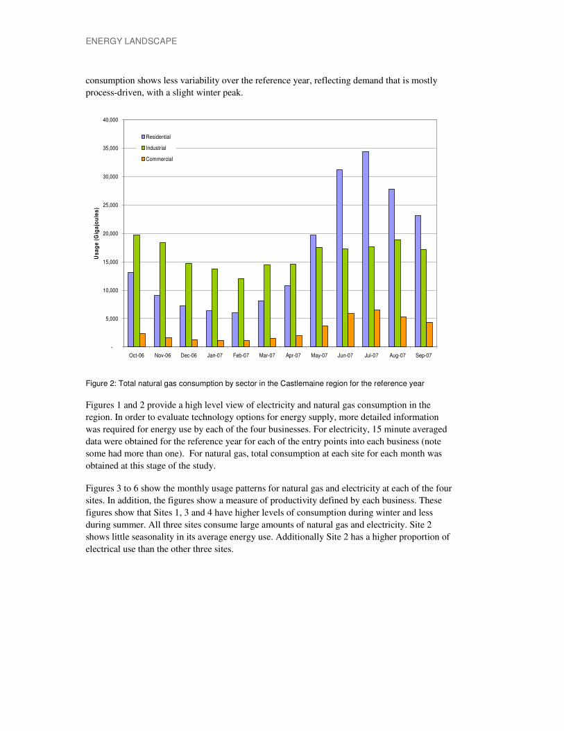
consumption shows less variability over the reference year, reflecting demand that is mostly
process-driven, with a slight winter peak.
-
5,000
10,000
15,000
20,000
25,000
30,000
35,000
40,000
Oct-06 Nov-06 Dec-06 Jan-07 Feb-07 Mar-07 Apr-07 May-07 Jun-07 Jul-07 Aug-07 Sep-07
Us
ag
e (
Gig
ajo
ule
s)
Residential
Industrial
Commercial
Figure 2: Total natural gas consumption by sector in the Castlemaine region for the reference year
Figures 1 and 2 provide a high level view of electricity and natural gas consumption in the
region. In order to evaluate technology options for energy supply, more detailed information
was required for energy use by each of the four businesses. For electricity, 15 minute averaged
data were obtained for the reference year for each of the entry points into each business (note
some had more than one). For natural gas, total consumption at each site for each month was
obtained at this stage of the study.
Figures 3 to 6 show the monthly usage patterns for natural gas and electricity at each of the four
sites. In addition, the figures show a measure of productivity defined by each business. These
figures show that Sites 1, 3 and 4 have higher levels of consumption during winter and less
during summer. All three sites consume large amounts of natural gas and electricity. Site 2
shows little seasonality in its average energy use. Additionally Site 2 has a higher proportion of
electrical use than the other three sites.

ENERGY LANDSCAPE
7
0
50
100
150
200
250
0
2,500
5,000
7,500
10,000
12,500
15,000
17,500
20,000
22,500
Oct-06 Nov-06 Dec-06 Jan-07 Feb-07 Mar-07 Apr-07 May-07 Jun-07 Jul-07 Aug-07 Sep-07
Pro
du
cti
ivit
y (
kg
/GJ)
En
erg
y c
on
su
mp
tio
n (
GJ)
Site 1: Energy consumption and productivity
Electricity
Gas
Productivity
Figure 3: Site 1, monthly energy usage and productivity during the reference year
0.00
5.00
10.00
15.00
20.00
25.00
0
200
400
600
800
1,000
1,200
1,400
1,600
1,800
2,000
Oct-06 Nov-06 Dec-06 Jan-07 Feb-07 Mar-07 Apr-07 May-07 Jun-07 Jul-07 Aug-07 Sep-07
Pro
du
cti
vit
y (
fou
nd
ary
la
bo
ur
ho
urs
/GJ)
En
erg
y c
on
su
mp
tio
n (
GJ)
Site 2: Energy consumption and productivity
Electricity
Gas
Productivity
Figure 4: Site 2, monthly energy usage and productivity during the reference year

ENERGY LANDSCAPE
0
10
20
30
40
50
60
70
0
1,000
2,000
3,000
4,000
5,000
Oct-06 Nov-06 Dec-06 Jan-07 Feb-07 Mar-07 Apr-07 May-07 Jun-07 Jul-07 Aug-07 Sep-07
Pro
du
cti
vit
y (
kg
/GJ)
En
erg
y c
on
su
mp
tio
n (
GJ)
Site 3: Energy consumption and productivity
Electricity
Gas
Productivity
Figure 5: Site 3, monthly energy usage and productivity during the reference year
0
1
1
2
2
3
3
4
0
1,000
2,000
3,000
4,000
Oct-06 Nov-06 Dec-06 Jan-07 Feb-07 Mar-07 Apr-07 May-07 Jun-07 Jul-07 Aug-07 Sep-07
Pro
du
cti
vit
y (
bed
-da
ys/G
J)
En
erg
y c
on
su
mp
tio
n (
GJ)
Site 4: Energy consumption and productivity
Electricity
Gas
Productivity
Figure 6: Site 4, monthly energy usage and productivity during the reference year
The 15 minute electricity data highlight further issues relating to the energy use by the four
businesses, these can be observed in Figure 7. In this figure it is apparent that Site 1 consumes
by far the most electricity with a definitive weekday/weekend split in consumption. Sites 3 and
4 show a similar pattern of repeatable weekday usage, with reduced consumption on weekends.
Site 2 shows a consistent baseline similar in magnitude to Site 3 but also shows large transient
spikes associated with testing of very large pumps. These spikes can place stress on the overall

ENERGY LANDSCAPE
9
system and while treating them is beneficial to the grid, they represent only a small potential
saving in greenhouse gas emissions due to their relative infrequency.
Figure 7: 15 minute averaged electricity use for a 2 week period in October 2006. The two week period
was chosen to highlight the transient peaks at Site 2.

ENERGY LANDSCAPE
Table 1a provides a measure of the energy used at each site in the reference year. Table 1b
provides an estimate of greenhouse gas savings required by each of the four businesses to reach
their ambitious 30 per cent greenhouse gas reduction target. Both tables include a correction to
the Site 2 electricity total which was in error in the earlier reports. Those sites able to reduce
their electricity consumption will benefit more in this regard. Reduced electricity use
significantly decreases the greenhouse gas emissions due to the high emission associated with
grid based electricity (mostly brown coal derived) and the large losses in the transmission and
distribution of electricity to Castlemaine. Table 1c presents the productivity for each site
divided by the annual CO2 emissions and energy use. These values provide a baseline for future
comparisons which allow the environmental performance of each business to factor in changes
in production.
Table 1a: Total energy usage (GJ/year), reference year
Site 1 Site 2 Site 3 Site 4 Total
Natural Gas 145 332 5 128 25 199 29 324 204 983
Electricity 81 980 11 096 9133 7644 165 542
Coking Coal 8434 8434
Total 227 312 24 658 34 332 36 968 323 270
Note: Coking coal usage is not tracked directly, so the figure is an estimate based on averaged amounts ordered.
Table 1b: Total CO2 emissions (tonnes/year), reference year
Site 1 Site 2 Site 3 Site 4 Total
Natural Gas 8298 293 1439 1674 11 704
Electricity 36 650 4722 4083 3418 48 873
Coking Coal 928 928
Total 44 948 5943 5522 5092 61 505
Savings required 13 484 1782 1656 1528 18 450
Note: Coking coal usage is not tracked directly, so the figure is an estimate based on averaged amounts of coke ordered.
Table 1c: Emissions, energy use and productivity for the reference year
Productivity measure Site 1 Site 2 Site 3 Site 4
Emissions 918.7a 38.7c 229.2e 15.2g
Energy 181.6b 9.3d 36.9f 2.1h a kg product / tonne CO2 b kg product / GJ c labour hours / tonne CO2 d labour hours / GJ e kg product / tonne CO2 f kg product / GJ g bed days / tonne CO2 h bed days / GJ

OPTIONS DEVELOPMENT
11
2. OPTIONS DEVELOPMENT
In Stage 2 of this study a number of options were investigated using renewable and fossil fuel
systems for local energy supply. Local energy was chosen as the primary focus to allow each
business to control their own supply and to potentially increase their efficiency through
cogeneration.
2.1 Technology options
In Stage 2 of this study an economic analysis was performed for solar thermal, solar
photovoltaic, wind turbine and natural gas based combined heat and power (CHP) systems for
the production of electricity and/or hot water.
Table 2 provides the characteristics of the systems considered, while Table 3 provides an
indication of energy generation costs. The systems using wind and solar are modular and as
such can be scaled either up or down accordingly for cost and greenhouse gas savings (Table 4).
Table 5 provides an indication of discounted payback time. Results in this table show that CHP
and solar thermal evacuated tubes provide reasonable payback times, while solar PV and wind
are less favourable due to the geographical location of the study area.
Table 2: Scale and characteristics of various options
Technology Site 1 Site 2 Site 3 Site 4
CHP Cogeneration
Two plants at existing site (2x 1.9 MWth) and one at the planned expansion (3 MWth)
N/A One plant on site (0.9 MWth)
N/A
Solar Thermal N/A N/A a. Parabolic trough collector (4,000 m2).
b. Evacuated tube collector (2,666 m2, aperture area)
Roof-mounted flat plate collectors (45 m2).
Wind (large) A single 3 MW wind turbine
Wind (small) Twenty-five 10 kW wind turbines (250 kW in total)
Solar PV Modular 250 kWp polycrystalline array
aScaled to match thermal power demands on each site.

OPTIONS DEVELOPMENT
Table 3: Cost of generating energy for various options (c/kWh)
Technology Site 1 Site 2 Site 3 Site 4
CHP Cogeneration 5.3 - 9.5 N/A 7.3 - 9.6 N/A
Solar Thermal N/A N/A a. 3.3
b. 1.6
6.1
Wind (large) 13.2
Wind (small) 85.0
Solar PV 29.6
Table 4: Greenhouse gas emission savings (tonnes per year)
Technology Site 1 Site 2 Site 3 Site 4
CHP Cogeneration 35 465a N/A 1987 N/A
Solar Thermal N/A N/A a. 815
b. 815
4.6
Wind (large) 7464
Wind (small) 280
Solar PV 561
a GHG savings include the notional site expansion.
Table 5: Discounted payback for various options (years)
Technology Site 1 Site 2 Site 3 Site 4
CHP Cogeneration 3 - 7 N/A 3 - 5 N/A
Solar Thermal N/A N/A a. 21 - 34
b. 6 - 6
>100
Wind (large) 24 - >100
Wind (small) >100
Solar PV >100

OPTIONS DEVELOPMENT
13
2.2 Updates and changes to Stage 2 technology options
During Stage 2 of this study, the freeware program Cogen Ready Reckoner v 3.1 (Sinclair
Knight Merz, 2002) was used to assess the financial and environmental savings from the
installation of CHP at Sites 1 and 3. This program was used to allow similar studies to be
performed elsewhere using the same methodologies. On further inspection a small number of
limitations became apparent. While emission rates for electricity production can be prescribed,
the emission rate for natural gas (and other fuels) used for the cogeneration plant are fixed
within the model. Thus site specific emissions for these fuels need to be post processed.
As noted in the two previous reports, the CO2 emission rate for grid based electricity in Victoria
(mostly derived from brown coal) is assumed to be 1.532 t/MWh in Castlemaine accounting for
transmission and distribution losses. Natural gas is assumed to have a CO2 emission rate of
0.057t/GJ accounting for upstream losses. Using these figures, the greenhouse gas savings in
Table 4 are updated and presented in Table 6 which shows a small degree of change (from the
assumptions of Cogen Ready Reckoner) and also shows contributions from each plant at Site 1.
In the Stage 2 report, greenhouse gas savings from exported electricity were not accounted for,
while greenhouse gas emissions from extra natural gas consumption were. The electricity
created by the combustion of natural gas onsite displaces grid based electricity with much
higher emission intensity. Table 7 presents results for greenhouse gas savings which also
include the impacts from displaced electricity. In this table it can be seen that Plant 1 at Site 1
and Site 3 savings are substantially increased. These extra savings are attributable to a poor
matching of thermal and electrical needs. In this case, the high thermal demand requires
generation of electricity above the needs of each premise. This result indicates that local natural
gas-fired generation is advantageous from a greenhouse gas reduction perspective. Indeed, any
local natural gas-fired unit with an electrical efficiency of only 14 per cent or above would
produce greenhouse gas savings. This is due to the inherently low efficiency of generation in
Victoria, which is further exacerbated by the large transmission and distribution losses to the
Castlemaine region.
Table 6: Updated greenhouse gas emission savings using location specific emission rates (tonnes per
year)
Technology Site 1 Site 2 Site 3 Site 4
CHP Cogeneration 5844a
11 193b
19 092 c
N/A
1951 N/A
Solar Thermal N/A N/A c. 815
d. 815
4.6
Wind (large) 7464
Wind (small) 280
Solar PV 561 a Plant 1 b Plant 2 c Plant 3

OPTIONS DEVELOPMENT
Table 7: Updated greenhouse gas emission savings (tonnes per year) using location specific emission
rates including displaced exported electricity
Technology Site 1 Site 2 Site 3 Site 4
CHP Cogeneration 13 872a
11 949b
22 492 c
N/A
5785 N/A
Solar Thermal N/A N/A e. 815
f. 815
4.6
Wind (large) 7464
Wind (small) 280
Solar PV 561 a Plant 1 b Plant 2 c Plant 3
For the Stage 2 report it was assumed that excess electrical generation from CHP units would
receive retail price for export. A business intending to export electricity into the local grid does
so under a Network Connection Agreement with the local distributor (in this case Powercor)
and a contractual arrangement with their retailer. The agreement would typically cover the price
paid by the retailer, hours of operation, and total annual amount of electricity supplied. While a
CHP unit with export potential may provide the retail business a hedge against price volatility in
the NEM, the retailer must gauge this against their business interest and their perceived risk of
losing generation capacity at crucial times. The final price for export will be determined through
negotiations with the retailer and the generation proponent taking such factors into account.
Table 8 provides a sensitivity analysis for payback times by setting a price for export as a
percentage of the retail price. While the price for export in the Stage 2 report was on the
optimistic side, little difference is apparent for any plant at Site 1. At Site 3 the change is more
pronounced as this business has significantly higher heating demands resulting in a large
amount of electricity export.
Table 8: Discounted payback rates (nearest year) for CHP options with varying degrees of retail price for
exported electricity
Technology Site 1
(Plant 1)
Site 1
(Plant 2)
Site 1
(Plant 3)
Site 3
100% Retail 3 – 5 4 – 7 3 – 5 3 – 5
80% Retail 3 – 6 4 – 7 3 – 5 4 – 7
60% Retail* 3 – 6 4 – 7 3 – 5 5 – 10
*Currently the annual average wholesale price in Victoria (~$46/MWh) which is approximately 60% of peak retail price for these two businesses.

OPTIONS DEVELOPMENT
15
A number of the businesses expressed interest in having a combination of technologies to meet
their greenhouse gas reduction targets. To this end, Table 9 presents payback calculations for
those sites able to use CHP with a combination of solar PV and/or wind turbines. Only electrical
generation has been considered as the thermal needs of the sites have been provided by the
proposed CHP plant. In this table slight variations are apparent for the CHP only estimates
compared with the Cogen Ready Reckoner estimates due to averaging of the data.
In this table it is obvious that a reasonable level of renewable technologies can be added to an
overall package without substantially altering the payback times. When packaged as an overall
solution the renewable options appear more favourable than when considered in isolation. All
options presented in this table have a positive NPV and an IRR above 15 per cent (for both the
low and high cases) which could be broadly considered a reasonable investment, although many
businesses consider 20% a minimum value depending on the type of investment option.
One immediate and somewhat counterintuitive outcome of this packaging is that the investment
in extra capacity appears best for those sites (or plants) which export electricity. This result is
from the favourable revenue that could be received for export electricity (even at wholesale
price) due to the low price of gas. In this case, adding more electricity would be unwarranted for
the business needs but could be seen as potentially beneficial for the “greening” and security
(through generation diversity) of the wider network.
Table 9: Multiple technology options for each business (100% retail price for export)
Additional Renewable Additional CO2
savings (t/y)
Payback (High)
Payback (Low)
NPV (High)
NPV (Low)
IRR (High)
IRR (Low)
Site 1 (Plant 1)
CHP only 0 2 3 $5,560,867 $2,509,487 48.1 28.8
10kW Wind 11.21 2 4 $5,455,209 $2,396,530 45.5 26.9
20kW Wind 22.42 2 4 $5,349,561 $2,283,573 43.1 25.2
30kW Wind 33.63 2 4 $5,243,912 $2,170,615 41.0 23.7
50kW Wind 56.05 3 5 $5,032,616 $1,944,701 37.3 20.9
100kW Wind 112.1 3 6 $4,504,374 $1,379,914 30.1 15.5
10 kW Solar PV 22.44 2 4 $5,499,535 $2,432,309 46.0 27.3
20 kW Solar PV 44.88 2 4 $5,438,212 $2,355,131 44.1 25.9
30kW Solar PV 67.32 2 4 $5,376,889 $2,277,953 42.3 24.7
50 kW Solar PV 112.2 3 4 $5,254,244 $2,123,597 39.1 22.4
100 kW Solar PV 224.4 3 5 $4,947,630 $1,737,708 32.9 17.8
10kW Wind + 10kW Solar 33.65 2 4 $5,393,886 $2,319,352 43.6 25.6
20kW Wind + 20kW Solar 67.3 3 4 $5,226,915 $2,129,217 39.8 22.9
30kW Wind + 30kW Solar 100.95 3 5 $5,059,944 $1,939,081 36.6 20.5
40kW Wind + 40kW Solar 168.25 3 6 $4,726,002 $1,558,811 31.4 16.6
Site 1 (Plant 2)
CHP only 0 3 5 $3,560,651 $1,176,564 35.6 18.0
10kW Wind 11.21 3 6 $3,455,003 $1,063,607 33.6 16.5

OPTIONS DEVELOPMENT
20kW Wind 22.42 3 6 $3,349,355 $950,649 31.7 15.2
10 kW Solar PV 22.44 3 5 $3,499,328 $1,099,386 34.0 16.9
20 kW Solar PV 44.88 3 6 $3,438,006 $1,022,208 32.5 15.8
10kW Wind + 10kW Solar 33.65 3 6 $3,393,680 $986,429 32.1 15.5
Site 1 (Plant 3)
CHP only 0 2 4 $8,457,047 $3,654,763 47.5 27.5
10kW Wind 11.21 2 4 $8,351,399 $3,540,805 45.8 26.3
20kW Wind 22.42 2 4 $8,245,750 $3,427,848 44.2 25.2
30kW Wind 33.63 2 4 $8,140,102 $3,314,891 42.8 24.2
50kW Wind 56.05 2 4 $7,928,805 $3,088,976 40.0 22.2
100kW Wind 112.1 3 5 $7,400,563 $2,524,190 34.4 18.2
10 kW Solar PV 22.44 2 4 $8,395,724 $3,576,585 46.1 26.6
20 kW Solar PV 44.88 2 4 $8,334,402 $3,499,407 44.9 25.7
30kW Solar PV 67.32 2 4 $8,273,079 $3,422,229 43.6 24.8
50 kW Solar PV 112.2 2 4 $8,150,433 $3,267,873 41.4 23.3
100 kW Solar PV 224.4 3 5 $7,843,819 $2,881,983 36.6 19.9
150 kW Solar PV 336.6 3 5 $7,537,206 $2,496,094 32.8 17.2
10kW Wind + 10kW Solar 33.65 2 4 $8,290,076 $3,463,627 44.5 25.4
20kW Wind + 20kW Solar 67.3 2 4 $8,123,105 $3,273,492 41.9 23.6
30kW Wind + 30kW Solar 100.95 3 4 $7,956,134 $3,083,357 39.6 21.9
40kW Wind + 40kW Solar 168.25 3 5 $7,622,191 $2,703,087 35.5 19.0
Site 3
CHP only 0 2 3 $2,959,035 $1,379,616 49.4 29.9
10kW Wind 11.21 2 4 $2,853,387 $1,266,659 44.5 26.4
20kW Wind 22.42 2 4 $2,747,738 $1,153,701 40.4 23.4
30kW Wind 33.63 3 5 $2,642,090 $1,040,744 36.9 20.9
50kW Wind 56.05 3 6 $2,430,793 $814,829 31.3 16.7
10 kW Solar PV 22.44 2 4 $2,897,712 $1,302,438 45.4 27.1
20 kW Solar PV 44.88 2 4 $2,836,390 $1,225,260 42.0 24.6
30kW Solar PV 67.32 3 4 $2,775,067 $1,148,082 39.0 22.5
50 kW Solar PV 112.2 3 5 $2,652,421 $993,726 34.1 19.0
10kW Wind + 10kW Solar 33.65 2 4 $2,792,064 $1,189,481 41.2 24.0
20kW Wind + 20kW Solar 67.3 3 5 $2,625,093 $999,345 35.2 19.6
30kW Wind + 30kW Solar 100.95 3 6 $2,458,122 $809,210 30.5 16.2

OPTIONS DEVELOPMENT
17
2.3 Alternative options
2.3.1 Green power purchases
Only one of the four businesses currently purchases green energy. Using the independent
organisation green electricity watch (http://www.greenelectricitywatch.org.au ) as a guide, the
average additional price (above the standard contract rate) for the 6 retail packages rated very
good (in Victoria) is around 4.97 c/kWh for 100 per cent accredited green power.
The selection of green power options is not simple. The star rating provided by green electricity
watch is based on responses to a detailed questionnaire and interview. These factors determine
the extent to which the purchases use existing sources and the percentage of total sales that are
derived from green sources (i.e. the degree to which the product is driving the market forward).
Retailers charge for green power in a number of ways. Firstly they can charge per unit of power
used, for instance if a 10 per cent green power option is chosen, the bill will be charged 90 per
cent at the standard retail rate and 10 per cent at the retail rate plus a green power premium.
Some options are sold as a fixed amount of green power at a fixed rate, and some retailers
charge a fixed amount but the consumer receives a variable amount of green power equal to a
percentage of power use.
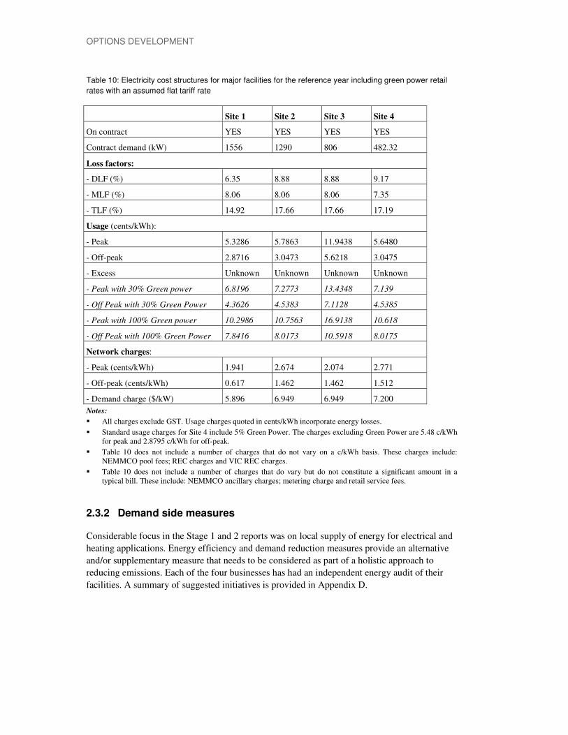
Table 10 displays the current contract rate for the businesses and includes an estimate of the
retail rate if the businesses were to adopt green power assuming a variable premium payment of
4.97 c/kWh. It is possible through negotiation that the businesses could obtain a cheaper rate
given their large energy use. For example the rate paid by Site 4 indicates a premium payment
of 3.4 c/kWh. For the purpose of this analysis however, the value chosen is based on the price
of the highest rated variable tariff products for 100 per cent green power listed by green
electricity watch. It is assumed that the same premium is applicable to a 30 per cent purchase.
These results provide a comparison for the businesses to consider against the cost of local
generation. Referring to Table 3, it is obvious that only the CHP and solar thermal evacuated
tube (for hot water) technologies are comparable or cheaper than the green power purchase.
Additionally the green power purchase does not involve additional capital expenses. While this
would indicate that green power is a more promising option than local generation, there are a
number of network issues that need consideration. Primarily if the network is under or
approaching constraint (as is the case in Castlemaine) then purchasing green power can only be
viable through upgrades to the local network which will increase the cost of supply. Local
generation on the other hand may remove the need for augmentation resulting in lower
electricity costs. Furthermore, simply buying green power does not provide incentive to deal
with efficiency gains through better use and control of local load devices.
OPTIONS DEVELOPMENT
Table 10: Electricity cost structures for major facilities for the reference year including green power retail
rates with an assumed flat tariff rate
Site 1 Site 2 Site 3 Site 4
On contract YES YES YES YES
Contract demand (kW) 1556 1290 806 482.32
Loss factors:
- DLF (%) 6.35 8.88 8.88 9.17
- MLF (%) 8.06 8.06 8.06 7.35
- TLF (%) 14.92 17.66 17.66 17.19
Usage (cents/kWh):
- Peak 5.3286 5.7863 11.9438 5.6480
- Off-peak 2.8716 3.0473 5.6218 3.0475
- Excess Unknown Unknown Unknown Unknown
- Peak with 30% Green power 6.8196 7.2773 13.4348 7.139
- Off Peak with 30% Green Power 4.3626 4.5383 7.1128 4.5385
- Peak with 100% Green power 10.2986 10.7563 16.9138 10.618
- Off Peak with 100% Green Power 7.8416 8.0173 10.5918 8.0175
Network charges:
- Peak (cents/kWh) 1.941 2.674 2.074 2.771
- Off-peak (cents/kWh) 0.617 1.462 1.462 1.512
- Demand charge ($/kW) 5.896 6.949 6.949 7.200
Notes:
� All charges exclude GST. Usage charges quoted in cents/kWh incorporate energy losses.
� Standard usage charges for Site 4 include 5% Green Power. The charges excluding Green Power are 5.48 c/kWh for peak and 2.8795 c/kWh for off-peak.
� Table 10 does not include a number of charges that do not vary on a c/kWh basis. These charges include: NEMMCO pool fees; REC charges and VIC REC charges.
� Table 10 does not include a number of charges that do vary but do not constitute a significant amount in a typical bill. These include: NEMMCO ancillary charges; metering charge and retail service fees.
2.3.2 Demand side measures
Considerable focus in the Stage 1 and 2 reports was on local supply of energy for electrical and
heating applications. Energy efficiency and demand reduction measures provide an alternative
and/or supplementary measure that needs to be considered as part of a holistic approach to
reducing emissions. Each of the four businesses has had an independent energy audit of their
facilities. A summary of suggested initiatives is provided in Appendix D.

OPTIONS DEVELOPMENT
19
2.4 Preferred options
2.4.1 Site 1
After the Stage 2 report, the Site 1 business considered CHP as a serious candidate to meet their
greenhouse gas targets and to accommodate for expansion of their business. Between the Stage
2 report and the current Stage 3 report, the business engaged a consulting firm to detail more
exactly the costs, system performance and network issues for this option. Through this
engagement, the business has found that the full cost for deployment of CHP including factors
such as civil engineering, water treatment, steam reticulation, supplemental gas firing and high
voltage switch gear etc is closer to $1500 to $2000/kW (compared to $1100/kW assumed in the
Stage 2 report). It should be noted that the final cost of installation can vary considerably
depending on the vendor supplying and installing the machine. This is a major consideration in
the tendering process and is likely to contribute more significantly to the cost effectiveness of a
solution than performance differences of componentry between suppliers.
Table 11 presents payback calculations using Cogen Ready Reckoner assuming an installation
price of $1500/kW. In this case the results show that the payback time increases by around 1 to
2 years overall.
The use of waste to create biogas was considered in the Stage 2 report. Preliminary calculations
for the facility suggest that it would be economically feasible primarily due to the large costs for
dumping. Further analysis from the Site 1 staff has indicated that the high nitrogen content of
their waste is likely to decrease the energy output and hence the economic viability of the plant.
The system and others such as plasma arc technology remains of interest to the business in the
longer term but is not being considered for this current project.
Site 1 has also expressed an interest in a number of smaller local renewable options such as
solar PV for lighting. The business is considering these options against other passive measures
such as extensive use of sky lights for instance in the design of their expanded facilities.
Table 11: Discounted payback rates (nearest year) for CHP options with varying degrees of retail price for
exported electricity assuming an installation cost of $1500/kW
Technology Plant 1 Plant 2 Plant 3
100% Retail 4 – 6 5 – 9 4 – 7
80% Retail 4 – 7 5 – 9 4 – 7
60% Retail* 5 – 8 5 – 9 4 – 8
*Currently the annual average wholesale price in Victoria (~$46/MWh) is approximately 60% of peak retail price for these two businesses.

OPTIONS DEVELOPMENT
2.4.2 Site 2
Discussions with Site 2 staff after the release of the Stage 2 report confirmed that it may be
possible to reclaim some of the energy used during their pump testing. A conceptual model for
the reclamation is shown in Figure 8. In the current system an electrical motor is used to drive
the pump under test (red). A load is placed on the pump via a control valve before water is
returned to a large tank in which the water is stored and extracted for use. In the proposed
system, the control valve is replaced by pump (green) run in reverse. Electrical energy
reclamation and flow control is achieved through the attached motor.
Current System
Proposed System
Figure 8: Proposed energy reclamation system for Site 2
To estimate the potential of this energy reclamation system, it is assumed that the electrical
motors are 95 per cent efficient and that the pumps are 85 per cent efficient. In this case the total
system efficiency should be around 65 per cent (i.e. 95% x 85% x 85% x 95% for the four
stages). Referring to Figure 7 it can be seen that testing of the large pumps can be in the order
1.8 MW electrical load (above the baseline). In this case, with a suitably sized pump and motor
combination, the reclamation could be around 1.2 MW with the final amount varying by the
degree of control required.
Using a class C pump from this business as a guide, it is suggested that this arrangement could
be built (onsite) for around $615/kW of reclaimed energy. This value is similar in magnitude to
the installation of an onsite diesel generator. Assuming a cost of electricity and network use at
8.46c/kWh, the business could save around $100 per hour under these conditions with this
facility.
OPTIONS DEVELOPMENT
21
The Site 2 business does not pay for modern demand charges as it falls under a legacy tariff
arrangement. If the business were to have been billed with a modern tariff, by reducing peak
load by 1200 kW, the business would avoid network demand charges of around $8,400 per
month. This would represent a significant saving for the business and allow a strong business
case to be made for installation of the recovery device.
While the tariff arrangement removes some incentive for the business to install a recovery
system, there are considerable gains to be had for the local network business by dealing with the
large intermittent peaks. This is dealt with further in Section 3.1.6 which considers the role of
the AER’s proposed demand management incentive scheme (DMIS). Ignoring the potential of
the DMIS, under the current billing arrangement the network business and retailer experience
the cost that would have otherwise been passed on to the customer under a modern tariff. In this
case, it is expected that the avoided cost (or lost revenue for these businesses under a modern
tariff) is a reasonable estimate of their impost. Installation of this demand management system
could allow the network business in particular to offset system upgrades required to maintain
the overall stability of the network for the small number of hours the test procedure operates. It
can also reduce the impact of critical peak pricing for the retailer if the tests coincide with high
market prices. It should be noted however that these benefits need to be considered against the
risk of failure which for the DNSP in particular can result in significant financial impost if the
effects propagate throughout the network.
2.4.3 Site 3
Discussions with Site 3 staff indicated that they would be interested in options to reduce their
heating loads with a potential preference for a CHP solution. In the Stage 2 report, two options
were determined to be suitable for meeting their needs, those being CHP and solar thermal
evacuated tubes. Both options were developed on the understanding that the business required
hot water. Feedback and subsequent discussion with Site 3 staff indicated that natural gas was
used to generate hot water (by passing steam through coils in a heating vat) for the wool dying
process and hot air (~80 °C) for drying the wool. Discussions indicated that 8 to 10 vats were
processed each day and that each vat contained around 9000 L of water and 4000 kg of wool.
For each vat cold water is injected at the beginning of a cycle and warmed to around 95 °C over
30 minutes and then held stable for a further 40 minutes. The wool is then rinsed with cold
water. The wool is spun dry and then sent to the gas fired drier.
The most appropriate application of CHP for this business would appear to be to preheat the
water injected into the vats and to heat the air used to dry the wool. Given that both processes
occur below 100°C it is possible that hot water (or another liquid medium such as oil) could be
used as the heat transfer medium for both activities. Further by using a storage tank the losses
from mismatched timing between the heating processes could be minimised. As such the
assumptions from the Stage 2 report remain adequate for estimating the potential of CHP at this
site.
Similarly estimations for the evacuated tubes remain adequate although it should be noted that
because of the time variation of the business operations and the solar thermal outputs a storage

OPTIONS DEVELOPMENT
tank would be vital, and would need to maintain temperature overnight. In both cases a
supplementary natural gas fired boiler may be required to ensure adequate supply.
Following the findings from Site 1, Table 12 presents paybacks updating capital costs to
$1550/kW. This table shows an increase in the payback time by around 1 to 2 years. For this
business the price received for export electricity is more pronounced due to the potential for a
large amount of exported electricity.
Table 12: Discounted payback rates (nearest year) for CHP options with varying degrees of retail price for
exported electricity assuming an installation cost of $1500/kW
Technology Discounted Payback (years)
100% Retail 4 – 7
80% Retail 5 – 9
60% Retail* 6 – 11
*Currently the annual average wholesale price in Victoria (~$46/MWh) which is approximately 60% of peak retail price for these two businesses.
2.4.4 Site 4
Site 4 is a government health care facility. At the beginning of the project the facility purchased
5 per cent of its energy under a green power retail contract. Currently the business buys 15 per
cent of their electricity as green power. While a number of potential local generation options
were provided for this facility, their preferred option is a combination of green energy purchases
and energy efficiency savings (see Sections 2.3.1 and 2.3.2). A combination of these practices
will allow the business to meet its 30% savings target.
In some regard the government run facility is constrained in undertaking large capital purchases
due to the nature of their operations. For this facility the first option for capital purchases comes
from its operating allocation. This funding provides for day to day operations and up to $25,000
can be approved by the CEO. Purchases greater than this amount must be given board approval.
Given the nature of the facility, health related activities are given highest priority. Gains from
energy efficiency audits for instance would require justification on freeing financial resources
over the long term for use in the core business of health care.
The second option for funding is through the Victorian Department of Health infrastructure
grants. In general, proposals taken to the department are based on reducing risk associated with
interruption or loss of services vital to the core business of health care. Generally projects
submitted to the department range between $20,000 and $200,000. There may be some merit in
providing a CHP facility which provides hot water, steam and electricity to the site to increase
security of supply. This facility could in fact replace the current diesel emergency standby
generators, the cost of doing this however is likely to be well in excess of the normal range
submitted for these grants.

OPTIONS DEVELOPMENT
23
Emergency generators in hospitals are guided by Australian Standard AS/NZS 3009:1998 (AS,
1998). The rules specify units above 25 kW can be fuelled through either onsite or reticulated
supplies that can provide at least 24 hrs capacity at full load. Safety valves should be powered
from the cranking battery of the generator. The likelihood of damage by catastrophe (e.g. flood,
fire, earthquake etc) should be considered when determining emergency supply. The AS 3009
suggests the following order (ascending) of reliability:
� One feeder from the electricity supply authority.
� Two independent feeders from the electricity supply authority.
� Two external sources of energy, i.e. a feeder from the electricity supply authority
and on-site generation of electricity from reticulated gas.
� On-site generation of electricity and an on-site emergency generator.
These Australian Standard suggestions indicate that a grant based on security of supply and
increased efficiency may be warranted. Furthermore, the system seems ideal given the rather
steady and predictable energy use by this facility (see Figure 7). Annual consumption data
(Figure 1a) are similar to Site 3 which suggests that considerably more natural gas is used than
electricity, and that a CHP unit matched to thermal needs would export a considerable amount
of electricity. A unit matched to the electrical needs would still provide substantial greenhouse
gas savings and would be far cheaper.
The final option for capital funding are government grants and in many cases the primary
motivation may be environmental (e.g. reduction in greenhouse gas emissions) rather than the
health based outcomes. Examples of schemes relevant to this project which could be considered
avenues in this regard are provided in Section 5.

OPTIONS DEVELOPMENT
2.4.5 Summary
Table 13 provides a simple summary of options preferred by each business. It should be noted
that this summary is only a reflection of the businesses preferred options and selection and
uptake of any options developed in this study will be determined by each business after
consideration of the issues noted in the Stage 1, 2 and 3 reports and those issues faced by each
individual business in their day to day operations. Additionally more than one option may also
be applicable for the same process (for instance hot water from solar thermal or CHP). While
each business joined the partnership model with the ambitious target of a 30% reduction in
greenhouse emissions by 2010 in good faith, at the time of writing the worldwide economic
downturn may cause a re-evaluation on the timing of implementation of any options considered.
Table 13: Preferred technology options for each business
Technology Site 1 Site 2 Site 3 Site 4
CHP � � � � Solar Thermal
� � � �
Solar PV � � � �
Wind (large) � � � �
Wind (small) � � � �
Energy Efficiency Measures � � � �
Green Power Purchases � � � �

TECHNICAL ASPECTS
25
3. TECHNICAL ASPECTS
3.1 Network operations
As noted in the Stage 2 report, there are a number of issues relating to the impact of local
generation on the network that need to be considered. These issues relate to impacts on network
safety and reliability, changes in revenue and return on investment for the network operator, and
methods used to charge for upgrades to the network.
3.1.1 Connecting local power supply in the distribution network
A number of issues need to be considered by the DNSP when considering the introduction of
local generation to their low voltage (LV) and medium voltage (MV) network. Primarily the
DNSP needs to ensure that they maintain established levels of power quality, availability, and
reliability of the network at a reasonable cost. While the term ‘MV’ is technically inapplicable
in accordance with the Australian Standards, it is used here to exclude the high voltage
transmission and sub-transmission levels of the network (see Figure 9) which are owned and
operated by a transmission network service provider (TNSP). While local generation can lead
to effects in all levels of the transmission and distribution systems, in this report the focus is on
effects in the distribution system where they are most prominent.
The connection of local generation in the low voltage distribution system can lead to design and
control issues for network companies. This is primarily because the electricity grid was
designed to feed power in one direction from a few large generators to a large number of
consumers. In this section, a number of the issues facing a DNSP when connecting local
generation are briefly examined.
It is important to note that in regard to local generation, devices essentially fall into three classes
of generator: synchronous machine, induction machine and inverter-connected generators.
The synchronous machine is the backbone of electricity generation throughout the world. It is
an alternating-current machine whose average speed is proportional to the frequency of the
applied or generated voltage. The output frequency is determined by the rotational shaft speed
and the number generator poles. Synchronous machines are commonly used as generators in
large power systems such as turbine generators and hydroelectric generators. Because the rotor
speed is proportional to the frequency of excitation, synchronous motors can be used in
situations where constant speed drive is required.
Synchronous machines have the capacity to deliver and sustain fault currents which can exceed
the rated current by several orders of magnitude. A fault current is an abnormal current in
circuit due to a fault (usually a short circuit). The maximum (making current) fault occurs in the
first 20 ms while the steady state fault current follows after approximately 40-60 ms. To protect
a circuit, the fault current must be high enough to operate a protective device as quickly as
possible. The protective device must be able to withstand the fault current. A calculation of fault

TECHNICAL ASPECTS
currents in a system determines the maximum current at a particular location. The value
determines the breakers and fuses required to ensure a rating equal to or greater than this value.
Asynchronous (or induction) machines (AMG) can be operated at a range of speeds. The rotor
in this case must be driven at a speed higher than the grid frequency in order to deliver power to
a network. The capacity to generate at variable speeds lends the AMG to renewable energy
applications where the primary energy source is variable. Large wind turbines are an example
technology.
AMG’s require an external supply to provide excitation. Depending on the speed of the rotor,
the excitation flux will either consume power (as a motor) or deliver power at the synchronous
frequency (as a generator). For a grid connected device, the excitation flux current is supplied
from the network which results in the generator requiring reactive power. The requirement of
real power from the network is a cost that needs to be factored into consideration. Since these
generators do not have self-excitation they are incapable of delivering sustained fault currents
but their making current needs to be accounted for.
For devices that output a direct current (DC) such as a photovoltaic cell, an inverter is required
to transform the output to an alternating current (AC) when connecting to the wider grid. A
power converter interfaces the generator’s variable DC output to the fixed AC grid signal. At
larger scales, AC rotating machines are used operating at variable speed and a power converter
is used to interface the variable-frequency, variable-voltage AC signal with the fixed AC grid.
Like induction machines, inverters will not deliver steady state fault currents. Both will deliver
'making' fault current - in the case of inverters, at a similar level to normal operation, in the case
of induction machines, at a similar level to locked rotor start-up (say 6 times normal current;
westernpower, 2008).

TECHNICAL ASPECTS
27
Figure 9: Scehematic representation of a radial network

TECHNICAL ASPECTS
3.1.1.1 Voltage Control
In the transmission of electrical energy, the role of the distribution network is to deliver energy
from a zone substation directly to the consumer. Distribution feeders operate at medium
voltages (e.g. 22 kV) that directly supply MV loads or feed small distribution transformers
which step the voltage down to a lower voltage level. A distribution substation typically serves
several radial lines which provide power to local consumers (see Figure 9). The voltage on these
lines gradually decreases with distance and as such the voltage at the substation is set higher to
ensure the most distant consumer receives an adequate minimum voltage.
If a local generation unit is placed on the line with sufficient power such that the voltage can
rise above the substation level, then the DNSP will be unable to control the voltage. The
problem can be exacerbated by the fact that small units are non-dispatchable and as such are not
remotely controlled by the DNSP to match system load.
Another issue can be balance between the phases when a generating unit is connected to one
phase of the system. In this case, a voltage level increase on one phase may lead to an
imbalance between all three phases. A simple solution is for local generation to be three phase
connected. This is generally not an issue for large units (e.g. a CHP plant). Cost impediments
mean that smaller units such as solar PV however are likely to be single phase systems.
Installation of a large number could potentially lead to imbalances depending on their location.
3.1.1.2 Incident stability
Before allowing the connection of a local generator, the network operator must examine the
effects of a fault on the network. Consider a case where a local generator is located near the end
of an LV line. Normally there are interconnecting points in the LV system that allows
redundancy in the network under fault conditions. The number of these points will vary
considerably by region with more points expected in highly developed areas, and less in remote
locations. The circuit formed when using these interconnecting points is commonly longer than
the normal route. In this circumstance, the voltage at the local generation connection point will
rise and the unit may need to be disconnected to ensure the safety of other equipment on the
network.
If a change in frequency occurs in the network (from the loss of a large local generator for
instance), small local generating units with little inertia may not ride through the fault if the
spinning reserve in the system does not arrest the reduction in frequency quickly enough. In this
case, the units will disconnect and may potentially compound the problem. In this case it would
be necessary to carry an increased amount of spinning reserve in the system which will increase
the total cost of system operation.

TECHNICAL ASPECTS
29
3.1.1.3 Protection issues
Distribution network protection equipment is arranged for passive operation using settings
based on minimum fault currents while equipment sensitivities depend on maximum
prospective fault currents. In a traditional radial network, power flow is unidirectional (see
Figure 9) and fault currents are delivered from centrally located generators to the fault. Local
generation particularly in the form of synchronous machines provides additional sources of fault
current and the potential for bi-directional flow. To assess the impacts of local generation, the
DNSP needs to consider issues such as the maximum short circuit current, impedance relay
reach, power flow reversal, auto re-closure, and safety. If a proposed addition of local generator
causes significant change in this regard, the proponent may be required to pay for expenses
relating to system upgrades.
3.1.1.4 Power Quality
A DNSP is responsible for maintaining voltage levels between specified limits and ensuring the
quality of power remains within specified standards. This may be complicated by local
generation which could introduce many effects including voltage variation and harmonics.
Sudden changes in current injected into a network from local generation (from say a loss of a
CHP unit or large scale fluctuations in wind speed for wind turbines) or alternatively large
inrush currents from start-up operations can cause voltage dips.
Flicker (a variation of luminous flux from a lamp) can be caused by the voltage variation of
intermittent sources such as a wind turbine.
The power-electronics in local generation units can contribute to distortion of the network
waveform although the degree of distortion can be limited by local filtering and design.
Remote control signals distributed in the network to control, for example, the switching of
public lighting and day and night tariffs can be affected by some local generation units
especially wind turbines.

TECHNICAL ASPECTS
3.1.2 Energy flows and charges
The National Electricity Market (NEM) is a wholesale market for electricity supply in the
Australian Capital Territory and the states of Queensland, New South Wales, Victoria,
Tasmania and South Australia. It commenced operating in 1998 and delivers electricity to
customers on an interconnected power system more than 4000 km long. The NEM comprises
five regions that are based on State boundaries, with the ACT considered part of NSW.
Establishment of the NEM led to disaggregation of the vertically integrated government-owned
electricity authorities into separate generation, transmission, distribution and retail sales sectors
in each State (Figure 10). A gross pool spot market sets the short term (e.g. 5 minute) operating
levels and dispatchable resources (i.e. generators) by matching supply and demand. In doing so,
it sets a price for generation in each of the five regions every 30 minutes. The energy flows
through transmission lines (operated by a transmission network service provider; TNSP), to the
distribution system (operated by a distribution network service provider; DNSP), to the point of
end use. Large energy users (e.g. smelters etc) and energy retailers (collectively Market
Customers) purchase energy from the market and either use it onsite (in the case of large users)
or on-sell the energy to smaller end users (in the case of retailers). These market customers are
subject to volatile movements in the market price and can use a number of strategies such as
derivatives (which include swaps or hedges, options and forward purchased contracts), local
generation or demand reduction activities to shield themselves from these fluctuations.
For end users receiving their energy via a retail business, the retailer buys electricity at the price
determined by the spot market (ignoring strategies to reduce their exposure to market
fluctuations) and on-sells the electricity to them. The retailer pays the transmission and
distribution companies’ money for use of system charges (TUoS and DUoS) and the generator
for the electricity produced, it also pays the market operator (the National Electricity Market
Management Company; NEMMCO) charges associated with being a retailer. The generator
transactions are settled through NEMMCO, while the distributors are paid directly by the
retailer.
Other forms of energy production can exist. A non market generator (generally small units,
noting that units above 30 MW must participate in the NEM) could sell directly to a retailer for
instance. Alternatively, a retailer could own and operate a generation unit and sell electricity to
a customer. Similarly a business aggregating demand reduction activities could sell reductions
in load (equivalent to providing local generation) to a retailer. These alternative models are
beginning to be more widely adopted and form the basis for consideration of activities in this
study.
NEMMCO GENERATOR TNSP DNSPMARKET
CUSTOMER
Financial flow
Dispatch instructions
Energy flow
Figure 10: NEM energy and financial flows
TECHNICAL ASPECTS
31
3.1.3 Connection costs and charges
As noted in the Stage 1 report, the substation at Castlemaine is approaching its peak capacity.
Growth in the region, particularly rapid growth for instance from the expansion at Site 1, will
require significant network upgrades to ensure reliable energy service using standard network
development procedures.
Network utilities operate, maintain and upgrade their infrastructure based on forecast growth
over a 5 year cycle. These forecasts are used to determine the amount of spend required to meet
demand and are subject to regulatory checks. Previously Powercor’s economic operations were
regulated by the Essential Services Commission in Victoria (ESCV). As of 1 January 2009, the
state based regulatory operations were transferred to a national system run by the Australian
Energy Regulator (AER). While economic regulations are now operated at a national level, the
AER has used a legacy type arrangement whereby many of the previous state based
mechanisms have remained at least for the first determination (2011 to 2015 in Victoria) of the
AER.
The Regulatory authority decides how much Victorian DNSPs can receive in revenue by setting
a price cap for electricity sales. This cap represents the regulators view on what is reasonable
for Victorian DNSPs to charge customers for the delivery of electricity including maintenance,
operation and system reinforcement. This revenue forms part of the total electricity bill and is
known as the distribution use of system charge (DUoS). These prices are set at the beginning of
each five year determination. Currently the Victorian DNSPs are operating on the determination
set by ESCV for the period 2006 to 2010. The AER will set conditions for the next regulatory
cycle beginning in 2011.
A vital component of the regulators determination is a prediction of peak and base demand
provided by the DNSP. Any changes to the network within a regulatory cycle that result from
say demand side reductions or local generation can seriously affect this determination and short
falls in forecast throughput effectively operate as a penalty for the business under the price
capping scheme. Similarly, the introduction of a large load mid cycle (such as proposed by the
Site 1 expansion) can lead to significant concerns for the DNSP if their system does not have
sufficient redundancy built in.
Under the ESCV the cost of new and upgraded connections in Victoria was determined by the
“Electricity Industry Guideline, No 14: Provision of Services by Electricity Distributors”
(ESCV, 2004a). The guideline facilitates the determination of customer contributions to the
capital cost of new works and augmentation, the contestability of connection and augmentation
works, and the provision for excluded services. Embedded generation (distributed or local
generation in this study) falls under the excluded services in Guideline 14 and is guided further
by the “Electricity Industry Guideline, No 15: Connection of Embedded Generation” (ESCV,
2004b ). Guideline 15 is meant to provide clarity in the manner in which DNSPs negotiate and
set charges with distributed generation proponents and in determining payment of avoided use
of system charges (DUoS and TUoS). As noted earlier the AER is now responsible for the
economic determinations for distributors in each Australian State. In transferring functions to
the national level the AER inherited these guidelines and is responsible for their

TECHNICAL ASPECTS
implementation. While the AER is currently reviewing connection standards, it is likely that any
changes will be some time away due to the complex nature of the issue. As such it is expected
that these two guidelines will remain relevant to the study participants in their current form.
A contentious point in the connection of distributed generation has been the allocation of
“shallow” or “deep” connection costs. This has been raised in many submissions to government
authorities in reviews locally and abroad. The cost of connecting a local generator to the nearest
point in a network is referred to as a “shallow” connection charge. A circuit breaker used
exclusively by the generator for instance would fall into this category. This cost might not fully
reflect system reinforcement upstream which may be required to allow the safe implementation
of the device. These additional costs are considered by some as “deep costs” and in some areas
may be passed onto the proponent. Guideline 15 states that in Victoria shallow costs for the
connection are those associated with connection assets and any augmentation of the distribution
system up to and including the first transformation in the distribution system. Furthermore the
guideline states that deep costs beyond this point cannot be allocated to the local generator.
While reasonably simple in design, the issue can vary depending upon the timing of connection.
Consider a number of proponents that wish to connect to a network over time. The first
proponent may find that the system can easily cater for their introduction. Now at a later time a
second proponent may wish to connect to the network. In this case, the network’s ability to cater
for their introduction will have been altered by connection of the first proponent. In this case,
they may find that their proposed connection requires changes in the network such as
replacement of a circuit breaker at the next highest voltage level from increased fault levels for
instance. These costs which fall within the definition of a shallow charge may have been
avoidable by the second proponent if for instance, they had connected first, and if their addition
did not require augmentation for the earlier network state. Additionally a third proponent may
now find that adding to a network requires only standard costs because of changes brought
about by proponent two.
Clearly this is a complex issue determined by a number of factors including, the number of
proposed additions to a network, the forecast estimates used in the current determination, the
size of the proposed change and the degree of contingency available. It is worth noting here a
distinction between adding generation to a network and in undertaking local energy efficiency
measures. Adding local generation will require connection to the grid which incurs a connection
cost. In contrast, energy efficiency measures provide a reduction in demand (equivalent to
increased generation) which does not incur extra network costs. Both mechanisms can reduce
profits to retailers and DNSPs (those regulated by a price cap) through reduced volumes of
energy.
Dealing with these connection costs is an area of considerable and complex debate. In some
cases, the connection costs are seen as a barrier for introducing local generation. Some consider
this discriminatory given that existing large generators (formed under the previous integrated
government system) do not pay for their contribution to the network (e.g. fault currents etc)
which allows their energy to be delivered to the end user. In recent times however new large
scale generators have been liable for transmission upgrades.
Furthermore, issues around reliability and safety are a significant concern for network operators
who are responsible for the performance of their network and are penalised for inadequate

TECHNICAL ASPECTS
33
standards. Addition of generation (or demand reduction) within their network and outside their
scope of control can lead to significant risk. Valuing the change that local generation (or
demand management) provides for the network (positive or negative) is considered difficult to
determine, is location specific and has no currently available generalised method for evaluation.
In Victoria, Guideline 15 is used to assist in determining the portion of avoided DUoS from
local generation (note that local generation receives a full TUoS reduction).
In Australia, these issues are being considered via the Ministerial Council on Energy (MCE)
review on “Network Incentives for Demand Side Response and Distributed Generation” and the
Australian Energy Market Commission (AEMC) review of “Demand Side Participation in the
National Electricity Market”. A number of similar processes are underway abroad, one of the
most relevant being those under taken by Office of the Gas and Electricity Markets (Ofgem) in
the United Kingdom (see Ofgem, 2009).
3.1.4 Victorian DMIS
As an acknowledgement of the technical and policy barriers facing demand side solutions, the
AER have developed demand side incentive schemes (DMIS) for the NEM. Of direct relevance
to this study is the DMIS for Victoria (AER, 2009). At this stage, the DMIS in each state differs
reflecting in essence state based variations in policy prior to national regulation. The AER
intends to deliver a national version once influencing national policy settings such as CPRS and
reviews such as AEMC’s demand side participation are understood. Further discussion of DMIS
below relates specifically to the final Victorian determination as it is of most relevance to this
project.
The objective of the scheme is to provide incentives for Victorian DNSPs to implement efficient
non-network alternatives or to manage expected demand for standard control services in some
other way. It is not designed to be the primary source of funding for demand management
expenditure which is based on the approved forecasts of operating and capital expenditure in the
AER’s determination for a particular DNSP.
The scheme will provide a demand management innovation allowance (DMIA) which allows
the DNSP to recover funds allocated to these non network solutions through two mechanisms.
Part A of the DMIS allows “an annual, ex-ante allowance in the form of a fixed amount of
additional revenue at the commencement of each regulatory year of the regulatory control
period”. “In the second regulatory year of the subsequent regulatory control period, when
results for regulatory years one to five are known, a single adjustment will be made to return the
amount of any underspend on unapproved amounts to customers” to ensure the scheme remains
neutral. “The total amount recoverable under the DMIA within a regulatory control period will
be capped at an amount based on the AER’s understanding of typical demand management
project costs, and is scaled to the relative size of each DNSPs average annual revenue allowance
in the previous regulatory control period” (AER, 2009)
Part B of the DMIS allows the DNSP to “recover forgone revenue resulting from a reduction in
the quantity of energy sold for a DNSP”, “whose direct control services are subject to a form of
control whereby recovery of the annual revenue is at least partially dependent on energy sold.”
“The reduction in energy sold must be directly attributable to the implementation of a non-tariff
demand management program approved under part A of the DMIS. Approved forgone revenue

TECHNICAL ASPECTS
will be provided to a DNSP in the second regulatory year of the subsequent regulatory control
period, as an addition to the innovation allowance adjustment in that regulatory year, to offset
the disincentives associated with certain forms of control.” “Recovery under this part B is
limited to revenue forgone as a result of non-tariff demand management projects or programs
approved by the AER under the DMIA” (AER, 2009).
The DMIS is a potentially useful mechanism to realise the outcomes of this project particularly
for Site 2 which could implement a non network solution to a peak demand problem through the
use of a waste energy capture system (see Section 2.4.2). Any changes that might be
implemented through a DMIS would arrive slightly outside the window prescribed by this
project (30 per cent reductions in greenhouse gas emissions by 2010) due to the alignment of
the regulatory cycles. If proposed and accepted, it could be implemented at the beginning of
2011. This is the case with any proposed change that requires Powercor to participate directly to
facilitate the project outcomes. While not ideal, it is an unavoidable consequence of the
relatively long cycles used to regulate the network businesses.
3.1.5 Site 1
As noted earlier, since the release of the Stage 2 report, the Site 1 business has announced a
significant expansion (around twice the capacity) to their business. This potential was flagged in
Stage 2 and initial calculations of its impact were considered. To cater for the expansion, the
business found that it had three potential options for its energy supply, those being:
� Upgrades to the 22 kV Powercor substation at Castlemaine
� Installation of an on-site substation (22 kV) to be fed from a 66 kV line
� Installation of a cogeneration plant.
Upgrades to the existing substation and associated distribution equipment to handle the
proposed load would be significant. It is possible that the business would be required to pay a
component of this the upgrade cost. This capital contribution is developed on the principle that
customer contributions are required where the revenue expected from the customer over the
lifetime of the connection is less than the incremental cost of servicing the customer. The
incremental cost is the difference between the expected present costs of providing network
services with the customer, against those without the customer (ESCV, 2004a). The remaining
cost would be borne by the DNSP. This capital contribution from the DNSP would form part of
the asset base used in the submission to the regulator in their next determination.
Installation of an onsite substation to be fed from a passing medium voltage sub transmission
line (66 kV) was estimated at around $12 million. This upgrade would provide 20 MVA
capacity, an ample amount for Site 1’s energy security but with no additional environmental
savings.
Detailed costing analysis and further quotations for a cogeneration plant suggest a cost of
between $9 and $12 million for 6 MW of electrical capacity. The proposed system would be
built from three 2 MW units to deliver inbuilt redundancy. This system would require the
business to retain their current supply from Powercor.

TECHNICAL ASPECTS
35
The Site 1 business has indicated that the cogeneration option is their preferred scenario as it
provides them with substantial environmental savings and can be implemented in a timely
manner to facilitate expansion of their site. Preliminary discussions between Site 1 staff and
Powercor have indicated that fault current from the installation of the CHP plant is unlikely to
be an issue. Electricity supply from the cogeneration units are not intended to be exported.
3.1.6 Site 2
The peak demand solution noted in Section 2.4.2 may be a practical measure able to be
implemented under the Victorian DMIS. Preliminary discussions with Powercor have indicated
that this could be viable and that they will investigate its merit.
A number of factors need to be considered in this case. While Powercor could pay for the
development of an energy recovery system and recoup the costs through the DMIS, the system
itself falls outside the engineering expertise of the company. In this case, Site 2 staff would be
the most appropriate personnel to ensure the system is maintained and operated reliably. This
would require a contracting service arrangement with the Site 2 business to ensure optimal
operation. Alternatively it would require training of Powercor staff.
The proposed energy recovery device would need to be considered against standard network
options. Powercor has a thorough understanding of the reliability of these standard options. For
the proposed energy recovery system, the Site 2 business would need to use its expertise to
verify the operational abilities and reliability of their pumps. This would be necessary to ensure
sufficient comparisons can be made by Powercor with other alternatives. This is particularly
vital to ensure that risk to Powercor is minimised in the event of a failure of the proposed unit,
which could lead to disturbances elsewhere in the network. In this case, Powercor would be
penalised for reduced reliability and service of their network.
3.1.7 Site 3
Site 3 is also interested in a CHP solution. Because the business has heat loads well in excess of
their electrical requirements, an installation of a CHP unit to cater for their thermal needs (or a
portion thereof) would result in a significant amount of electricity exported to the grid. As for
any addition to the network, issues such as fault current levels, impacts on voltage from
start/stop operations etc would need to be investigated. Changes to fault current levels may
require upgrades to circuit breakers in the system depending on the current operational margins
of the network. The larger the fault current output by the unit the more likely this issue will be.
The level of fault current output by the unit is proportional to its size.
Given the disparity between electrical and heat loads for the Site 3 business, one option is the
introduction of a smaller unit to cater for electrical demand. Waste heat from the unit could still
be used to generate hot water or steam but would offset a smaller component of the overall heat
load. For a 200 kW unit, around 21 per cent of the heating load could be displaced compared to
around 67 per cent for the 834 kW unit.

TECHNICAL ASPECTS
Based on a yearly average of weekday loads, a 200 kW unit would save around 60 per cent of
greenhouse gas emissions. This compares to savings of around 93 per cent for the 834 kW plant
(49 per cent not accounting for export due to increased fuel use).
It is worth noting that the Site 3 business could achieve a greenhouse gas saving of 73 per cent
by offsetting all their electricity purchases with green power. The 834 kW option at $1500/kW
equates to a capital purchase of $1.25 million. The Site 3 business could afford to buy 10 years
of 100 per cent green power using the charge rates specified in Table 10. The CHP unit however
could be paid off in a quicker timeframe depending on the ability to negotiate the export
electricity price, and the difference in price of electricity and natural gas over time. After this
period the unit could be making a profit and in addition it could potentially save significant
network upgrade costs which haven’t been factored into the estimate.
A small microturbine which is less electrically efficient (e.g. 33% for a Capstone C200
compared with 40% for the Jenbacher engine based unit specified in the Stage 2 report) could
be useful for this site as it creates a high grade heat output. Given the clean burning of these
units, the hot exhaust could be used directly for drying the dyed wool with appropriate mixing
and control to ensure correct temperatures. While the microturbine may have some advantages
in this regard, the nominal cost of a microturbine is roughly 1.5 times its engine based
counterpart.
3.1.8 Site 4
Site 4 staff have not indicated a preference for a technology option that would result in direct
issues for the network. Their preference has been the purchase of green electricity and the
installation of energy efficiency measures aimed at reducing their use of natural gas and
electricity.
A CHP unit located at this site would have similar issues to Site 3 (i.e. high heat demand
resulting in exported electricity if matched to thermal load).

TECHNICAL ASPECTS
37
3.2 Resource sharing
3.2.1 Electricity supply
Each of the four businesses is currently joined to the distribution network owned and operated
by Powercor. Their electricity is obtained from generation at large remote sites which send their
output via the transmission and distribution networks. If one of the businesses were to install
local generation at their facility with export potential then demand on the substation would be
reduced and less power would enter the region. It is possible however that the network could
need augmentation to supply electricity by standard means in the event of failure. This could be
dealt with through other arrangement such as voluntary load shedding or using multiple smaller
units which reduces the overall risk albeit at additional cost.
One of the largest uncertainties in local generation is the price received for electricity supply.
The price that is received for the local electricity supply is determined through negotiation with
the energy retailer. It is expected that the price received is somewhere between the wholesale
and retail price. Some argue the price should be greater than wholesale because the local
generation can bring value to the network in terms of increased security and a potential
reduction in network upgrade costs presuming the equipment or procedure meets necessary
standards. This is particularly evident when considering peak load events. In this case, the
network is generally constrained in its ability to supply demand. In order to meet high customer
expectations, the traditional method to deal with the issue is to substantially upgrade the
network to cater for the few hours a year that peak load becomes critical. Local generation (or
demand reductions) can alleviate these costs by supplying energy close to or at the point of
load.
In some locations abroad (most notably Woking in the United Kingdom) the impediments of
connecting local generation to the network has brought about the installation of local “private
wire” networks (Jones, 2003). Physically this provides little difference (assuming that the
private network has a link to the larger grid at some location) to connecting the generation
source to the existing network. The main incentive in taking this approach is a reduction in
potential barriers and an ability to set more favourable prices for generation than through
negotiation with the local retailer.
In Australia, private wires exist on individual’s properties as shown in the example of Figure
11. These wires are owned by and are the responsibility of the property owner up to the point of
connection to the distribution network (Powercor, 2008). In Victoria, the safe operation of these
wires is governed by the Electrical Safety Act 1998 (ESV, 1998). The wires are inspected by the
local DNSP who issue notices if work is required on these lines.

TECHNICAL ASPECTS
Figure 11: An example of a private wire in the distribution grid
The private wire network as installed in Woking (and similar areas) generates and supplies not
only electricity, but also hot and cool water. In Woking, the model works with relative ease as it
has been setup as a public private partnership in the form of an environmental and energy
services company (ESCO). The ESCO is a wholly municipally owned non-profit making
company that delivers the local authority’s fuel poverty (minimising costs for vulnerable
residents) and environmental services. The company itself can enter into partnerships to deliver
these energy services to customers (Jones, 2003). Considerable effort was undertaken at the
beginning of the Woking process to investigate the legal frameworks required. To operate
within Australia, a similar legal and business structure would require investigation and
development.
An example of this process in Australia are the recent applications by GridX
(http://www.gridxpower.com/index.aspx) to build and operate developments in Greenfield
locations. In these developments, GridX propose to develop a service using gas engines that
provide electricity, hot and potentially chilled water supplies to consumers. In doing so they
seek to operate a vertically integrated monopoly consisting of combined generation, distribution
and retail.
Currently GridX own and operate a cogeneration facility in Glenfield NSW. At this location the
network is owned by a registered DNSP which receives energy from the cogeneration plant. A
retailer sells energy to the onsite customers.
The distinction between the ownership model employed at Glenfield and the proposed model is
important, as it forms the basis for determining whether registration is required under the
National Electricity Rules (NER). In the proposed model, GridX plans to own, operate and
control network infrastructure that is connected to another distribution system. As such, GridX
are required under the NER to register as a DNSP or seek exception from the AER. Registration
is designed to ensure that electricity network providers are subject to provisions of the NER
dealing with system security (chapter 4), network standards (chapters 5 and 7), pricing (chapter
6) and dispute resolution (chapter 8).
The AER can impose two types of exemption. First, a general exemption can be made.
Currently a number of facilities such as certain caravan parks, office buildings, flats, units and
apartments sharing common infrastructure, industrial parks and shopping centres are designated

TECHNICAL ASPECTS
39
this way. A general exemption by definition exempts compliance with chapter 5 of the NER
(AER, 2007). Second, the AER can grant a limited exemption which can exempt registration
but require compliance on specific conditions of chapter 5.
In submissions to the AER on the GridX proposal, a number of stakeholders commented on
issues they considered important when considering the proposed model. These included:
� Reliability and performance standards
� Technical and safety standards
� Setting of network charges and retail prices
� The applicability of retailer and distributor of last resort arrangements
� Informed consent
� Access to full retail competition
� Inconsistency with the AER’s NSP exemption guidelines
� Cooperation with long term network planning.
Some of these technical issues are discussed in Section 3 while other non technical issues such
as access to full retail contestability display the large degree of difficulty that could manifest
when considering an alternative business model for energy supply.
State based authorities have a direct role in regulating retail provision. States may also impose
their own consumer and protection arrangements such as implementing a price cap to ensure
consumers are not disadvantaged with respect to customers on traditional networks.
Additionally many of the safety obligations of DNSPs are contained in industry specific codes
that vary between jurisdictions.
AER (2007) in its deliberations on the proposed GridX model noted a large number of
conditions necessary to gain a retail licence in NSW as noted below. These licenses are granted
by the Minister for Energy in NSW based on recommendations from the Independent Pricing
and Regulatory Tribunal (IPART). These conditions are examples of those required in NSW. It
would be expected that each State has similar conditions. In Victoria, a retail licence is
governed by the “Electricity Industry Act 2000”.
� Prudential and credit support arrangements that must be observed by retailers
� Seeking to purchase energy from the wholesale electricity market
� Approved business-to-business procedures
� Pricing and price-control arrangements
� Standards of conduct for marketing arrangements

TECHNICAL ASPECTS
� Arrangements concerning the provision of information to customers
� The form of customer supply contract used to supply retail customers with
electricity and the matters that are required to be included within those contracts
� Telephone hotline arrangements for faults and difficulties with electrical works and
customer connection queries
� Mandated service levels for different categories of customer service queries
� Record-keeping requirements
� Customer transfer arrangements
� Commencement and discontinuance of supply arrangements
� Billing standards
� Meter testing arrangements
� Various reporting and compliance management obligations and dispute resolution
procedures.
To share excess electricity in the case of this study, the most obvious solution is the use of the
local existing distribution network. The price received for electricity supply to the local grid is
negotiated between the business owning the onsite generator (which could be a third party) and
the local retailer. Given the partnership model of the study, it is conceivable that a three (or
more) way negotiation could be arranged between the business exporting electricity, businesses
wishing to receive the exported electricity and the retailer to the mutual benefit of all parties.
If impediments in operating within the existing frameworks are considered too large, then
alternatives such as the GridX or Woking model could be considered. These may be significant
and costly exercises that require dealings and submissions to a number of relevant state and
federal authorities. In terms of this project, it is very unlikely the timeframes could be met
taking this route. Rather, it is suggested that the partnership model adopted in this study
provides a mechanism to ensure a more open and considered dialogue between the businesses,
retailers and local distribution network.

TECHNICAL ASPECTS
41
3.2.2 Heat supply
Sharing of heat resources is not governed by the same rules that govern electrical supply. It is
conceivable that heat in the form of hot water or steam could be produced at one of the four
sites and piped to the other sites. The piping would need to be placed underground and
depending on the sites may have to cross a major railway line. Furthermore, a contract of supply
would need to be formed which stipulated items such as the amount of hot water or steam
required, times of use, price for supply, reliability standards and contingencies plans etc.
Ignoring for the moment any cost impediments; the concept could be advantageous for a CHP
plant that produced more heat than was required for local use. In this study, the businesses
considered for CHP were provided estimates based on systems that matched (to as near as
possible given quotes received from vendors) their heating requirements. For Site 1, the heating
and electrical requirements were such that little export of either source was likely for Plant 2
and 3, and some excess electricity could be generated at Plant 1. At Site 3, matching thermal
load would create a large excess of electricity. If a CHP unit was located at Site 2 or 4 to
provide electricity, it could conceivably export a considerable amount of heat.
Heat loss from pumping low grade hot water is considerably smaller than from pumping high
temperature water or steam, since the loss is proportional to the temperature difference between
the medium and its surrounds. In addition, piping steam requires special treatment to trap and
remove condensate which can form due to the heat loss. While the loss can be minimised by
pumping low grade hot water, the energy savings are significantly reduced as less energy is
stored in the medium.
To a first approximation, heat loss from an insulated pipe can be estimated by Equation 1
(Cheng et al., 2006). This equation represents the steady state heat loss from an insulated pipe to
its surrounds. When buried underground, the temperature of the ground and its ability to
dissipate heat needs to be considered. Similarly, the transient effects for demand (and hence
flow) also need consideration. Estimates shown here are meant as a guide to the approximate
degree of loss that might be expected in steady sate conditions.
)D/Dln(
)TT(L2
inout
inoutkQ
−=
π (1)
Where;
Q is the heat loss (W)
k is the thermal conductivity (W/m°C)
L is the length of the pipe (m)
Din is the inside diameter of the pipe
Dout is the outside diameter of the insulated pipe
Tin is the fluid temperature
Tout is the ambient temperature

TECHNICAL ASPECTS
Table 14 presents the steady state heat loss estimates from a 1 m section of insulated pipe. The
thermal conductivity is assumed to be that of mineral wool (0.04 W/m°C; Tierling, 2009) and
the temperature differential is assumed to be 80 °C. These heat loss estimates can be thought of
as the supplemental heat required to maintain the temperature within the pipe. It is obvious from
this table that for a well insulated pipe the losses are moderate.
The distance between sites (see Figure 13, Table 15) assuming the pipe would follow a road is
around a kilometre. Referring to Table 14, it can be seen that the losses may be on the order of
10s of kilowatts. Assuming that an excess heat of around 500 kW is to be transferred then a loss
of around 25 kW represents 5 per cent of the total energy. Comparatively, electrical losses over
the same distance are much smaller. This is evidenced by comparing the losses in the entire
distribution system. For 2008-2009 the loss factor is 9.25% in this region (NEMMCO, 2008).
Given the electrical infrastructure already exists, clearly transferring energy in the form of
electricity is a preferable option assuming network arrangements and pricing are favourable.
Table 14. Heat loss estimates from an insulated pipe of various diameters (W/m)
Insulation Thickness
Pipe
Diameter 10 mm 20 mm 30 mm 40 mm 50 mm
30 mm 39.4 23.7 18.3 15.5 13.7
40 mm 49.6 29.0 21.9 18.3 16.0
50 mm 59.8 34.2 25.5 21.0 18.3
60 mm 69.9 39.4 29.0 23.7 20.5
70 mm 80.0 44.5 32.5 26.4 22.7
80 mm 90.1 49.6 35.9 29.0 24.8
90 mm 100.2 54.7 39.4 31.6 26.9
100 mm 110.3 59.8 42.8 34.2 29.0

TECHNICAL ASPECTS
43
Figure 12: GoogleEarth image of the study region showing Sites 1 to 4
Table 15: Distance between sites (m)
Site 1 Site 2 Site 3 Site 4
Site 1 0 1240 1110 770
Site 2 1240 0 460 920
Site 3 1110 460 0 710
Site 4 770 920 710 0
BUSINESS CONSIDERATIONS
4. BUSINESS CONSIDERATIONS
4.1 Business models
A number of business models are available for the installation, operation and maintenance of
local solutions for energy supply and use. These are briefly discussed in this section. The
methods used by the businesses will depend on their ability to spend on capital infrastructure,
their determination of risk and reward, and the in-house expertise in energy management.
4.1.1 Capital purchase
In a capital purchase arrangement, a technology vendor will provide a fixed cost for a complete
installation including project design, supply, installation and commissioning. In addition to this,
a service package can be offered that will operate and maintain the system throughout its life.
An advantage of this financing mode is that greater savings are achievable under this
arrangement. Options developed in this study are based on this approach.
4.1.2 Energy purchase
In an energy purchase arrangement, a technology vendor or third party may fully fund, or part
finance, the costs associated with the implementation of a plant, including the design, supply,
installation and operation of the scheme over a contract period. For renewable options, a vendor
may offer to supply a guaranteed level of energy supply.
The vendor would recover the initial capital costs and the ongoing maintenance charges over a
contractual agreement period, usually ten years, by charging a flat c/kWh for electrical output
and thermal output if applicable. Each specific project will have a unique c/kWh rate, dependent
upon a number of factors such as plant selection, project costs, maintenance prices, operational
hours and contract period. The benefits of this option include: no capital outlay entailing lower
risk; no ongoing maintenance costs; more immediate savings; and capped energy costs over the
contract period.
4.1.3 Green power
As noted in Section 2.3.1 a business may consider buying green power from a retailer rather
than locate generation on-site. It is not necessary for a business to buy green power from their
current retailer and in this regard the partnership model of this project may allow a coordinated
approach by the businesses with a retailer or a broker which allows them to negotiate a better
contractual price.
4.1.4 Retail solutions
Given the nature of this project, it is possible that an arrangement could be struck between the
businesses and a retailer which values the emission and network savings that could be achieved
with local generation. In this case, it might be possible that the retailer is able to provide a
business exporting cleaner electricity with a premium that is recouped through on selling to

BUSINESS CONSIDERATIONS
45
other business in the region (both to the other project partners and to other members of the local
community). This may provide the retailer a competitive market position by providing local
solutions for local problems. The retailer would need to assess how this compares with green
power options they may already sell, and how it may be used in the local region to hedge
against price volatility in the NEM. Further they would need to consider the impost of site
specific changes to standard business practices such as billing arrangements.
4.1.5 DNSP solutions
A number of the options discussed for this project can be of direct benefit to Powercor, the local
DNSP. While installation of a CHP plant might seem like an attractive non-network option to
cater for demand growth, the network business is not able to setup a plant under an energy
purchase arrangement for instance as it is not an energy retailer.
Section 3.1.6 detailed the possibility of a technology that could be developed for use by
Powercor to provide a unique local solution to a specific peak demand issue. This could utilise
the recent DMIS developed for Victorian DNSPs by the AER (see Section 3.1.4). This option
would require the business to consider a unique solution and to develop contractual
arrangements with a third party or develop in-house skills to ensure it was operated and
maintained in a fashion suitable for introduction on their grid.
4.1.6 Alternative energy supply solutions
The introduction of local supply and its ability to operate efficiently is contingent on favourable
arrangements with the local distribution company and with energy retailers. Alternative
business arrangements such as the Woking and GridX models discussed in Section 3.2.1 could
provide a solution if traditional routes are unfavourable. While conceptually simple, the
discussion in Section 3.2.1 details at a high level, the large number of issues that need to be
addressed with government authorities. To a large extent this is due to the small number of
precedents in this regard.
4.2 Energy use and productivity
In the Stage 1 report, the energy landscape was detailed to provide a base year for comparing
the results of any adoption undertaken by the project participants. A part of the analysis was a
measure of productivity which varied for each of the businesses. This was done to ensure that
future measures could factor in changes that could occur from either an expansion or
contraction in activity.
Since the release of the Stage 2 report, changes in the market has severely impacted the Site 3
business. The business has reduced its workforce by around one-third and then subsequently
reduced operations from a 5-day to a 4-day week. In this regard, they have easily achieved a 30
per cent reduction in emissions through demand reduction. This clearly shows the need to
consider energy use per unit of product or service delivered when considering the change in
emissions over time.
Likewise the Site 1 business has announced that it will have a two fold expansion in its
production. It is unfair to suggest that the business will double its greenhouse gas emissions as a

BUSINESS CONSIDERATIONS
result if it adopts alternative energy supply options. A final analysis of their impact needs to
factor the reduction in the energy intensity of production.
4.3 Carbon Pollution Reduction Scheme
The Federal Government released the exposure draft of the Carbon Pollution Reduction Scheme
(CPRS) legislation on 10 March 2009. The draft legislation follows on from the White Paper,
entitled Carbon Pollution Reduction Scheme: Australia's Low Pollution Future, which outlined
the Government's policy position on the Scheme's design. The Government has recently delayed
the start date for the scheme until 1 July 2011.
The structure of the CPRS has implications for the businesses that are considering natural gas-
fired cogeneration. Under the draft legislation, scheme obligations for greenhouse gas emissions
apply to operators of facilities that have direct (that is, on-site) greenhouse gas emissions of 25
000 tonnes of carbon dioxide equivalent (CO2e) a year or more. To illustrate these implications,
we consider two cases.
Case A
In Case A, we assume that the business continues with the same emissions profile as that in the
reference year. Table 1b shows that reference year direct greenhouse gas emissions (mainly
from the combustion of natural gas) place all the businesses below the 25 000 tonnes threshold.
As such, the business is not required to quote an obligation transfer number (OTN), and the
supplier of the fuel (i.e. the retailer) is liable for the emissions from the combustion of the fuel
by the business. The retailer will pass on these costs to the business (i.e. costs of the permits)
just as the retailer currently passes on network charges imposed by network operators. Given
the monthly billing cycle, this imposes increased cash outflow on a monthly basis.
Case B
In Case B, the business installs natural gas-fired cogeneration. Depending on the size of the
CHP, direct emissions may rise above the 25 000 tonnes threshold. If this is the case, the
business is regarded as a liable entity and must quote an OTN for a supply of fuel, transferring
scheme obligations from the retailer to the business. The company must now manage scheme
obligations (i.e. purchase permits equal to their emissions).
This has different cash flow implications compared to Case A. Under the draft legislation, the
business is required to surrender sufficient eligible emissions units to meet its obligation for a
financial year, by 15 December of the following financial year. This imposes compliance costs
on the business which were previously borne by the natural gas retailer. The business may
decide to purchase permits at different stages throughout the year depending on the spot price of
permits and its cash flow. The CPRS allows unlimited banking of permits and limited
borrowing of permits. Alternatively, the business can hedge its carbon price risk using carbon
futures markets.
Despite these cash flow implications regarding scheme coverage, the business case for on-site
natural gas-fired cogeneration is still a favourable one. This is because of the avoided carbon
costs by substituting emission intensive grid electricity (approximately 1.532 t/MWh) with low

BUSINESS CONSIDERATIONS
47
emission intensive natural gas-fired CHP (approximately 0.51 t/MWh assuming an electrical
efficiency of 40%).
Table 17 provides results for a hypothetical scenario for a business approaching the CPRS
threshold when using CHP. In this case, we consider a business whose yearly emissions from
CHP are 27 000 tonnes (~52 600 MWh @ 0.51 t/MWh). At full load and capacity this equates
to an installation around 6 MW in size. In the hypothetical scenario the business may choose to
run their facility at part load (say 90%) and obtain its extra needs from the gird. Furthermore,
we assume that the 6 MW is comprised of three 2 MW units. The business in this case may wish
to install two units instead to ensure it remains under the CPRS threshold and again obtain its
extra needs from the grid.
The Federal Government has made an unconditional commitment to an emissions allocation
that leads to a reduction in emissions of 5 per cent on 2000 levels by 2020 and 60 per cent
below 2000 levels by 2050. According to economic modelling conducted by Treasury, this
entails a carbon price of around $20 per tonne in 2010, increasing to around $36 per tonne in
2020.
As a ‘strongly affected industry’, the coal-fired electricity generation sector will benefit from
the Electricity Sector Adjustment Scheme and receive part of their requirements for carbon
permits for free. The allocation of free permits, the availability of international credits, hedging
and the structure of power purchase agreements between generators and retailers makes it
difficult to determine the degree of pass-through of carbon prices to the end-user.
Table 16 shows the CPRS costs for a hypothetical CHP facility assuming different degrees of
pass-through from electricity retailers but 100% pass-through from natural gas retailers over the
ten year period 2010 to 2020.
Table 16: CPRS costs over a ten year period for a hypothetical CHP facility
Site
Emissions
Total
Emissions
Cost
(PT 0%)
Cost
(PT 80%)
Cost
(PT 100%)
3 Units 27 000 27 000 $8,350,000 $8,350,000 $8,350,000
3 Units at
90% load
24 300 32 201 $7,520,000 $9,475,000 $9,950,000
2 Units 20 250 40 265 $6,265,000 $11,220,000 $12,500,000
PT = pass-through
The results clearly show that by avoiding the CPRS threshold, the business increases its
greenhouse emissions significantly as it replaces cleaner local natural gas-fired electricity with
more emission intensive grid based electricity which includes transmission and distribution
losses. With full pass-through of carbon prices its costs are significantly higher operating 2
units of CHP. However, operating 3 units at 90% load instead of 3 units at full load may reduce
its overall costs if CPRS compliance costs (staffing, working capital etc) over the ten year
period are estimated to exceed $1.6 million. Clearly, with no pass-through, business as usual is
the most attractive financial option.

BUSINESS CONSIDERATIONS
4.4 Regional Development Victoria Water and Energy Efficiency Initiative
The Water and Energy Efficiency Initiative is administered by Regional Development Victoria.
The program will provide $10 million over two years toward the cost of capital works to enable
industry to become more efficient in its use of water and energy.
Projects will need to demonstrate water or energy savings:
Water: A reduction in demand on potable urban water supplies, or the demand on a shared raw
water resource, or a lowering of the industry’s water usage per unit of output.
Energy: A lowering of energy usage, or energy related emissions, per unit of output.
Grants are primarily targeted at companies in the manufacturing and processing industries
located in regional Victoria and as such Site 4 may not be eligible.
Energy efficiency projects can include one or a number of supply or demand management
measures:
� Supply management: Involves projects that are capable of substituting one form of
energy for a more efficient one, e.g. using natural gas for boilers rather than mains
electricity.
� Demand management: Involves reductions in energy usage, internal waste heat
recovery, or a change in the manufacturing process that reduces energy demand
and/or substitution to a more efficient energy source.
Note this program also supports water saving initiatives.
Grants are only available to projects with an internal payback greater than three years and are
limited to 50 per cent of the total project capital cost or the amount required to reduce the
payback period to three years, whichever is the lesser.
Regional Development Victoria (RDV) has adopted benchmark capital costs for water and
energy projects. Funding requests that approach or exceed RDV’s adopted benchmark capital
cost will need to demonstrate that they have greater potential for investment attraction, job
creation, exports, or import replacement, and/or satisfy the following additional criteria:
� Environmental criterion: There are local water resource constraints, or energy
distribution capacity constraints that preclude lower cost alternatives.
� Technical criterion: There are site-specific engineering, water quality, or energy
supply stability requirements.
BUSINESS CONSIDERATIONS
49
It is possible that this funding mechanism could be used to assist the businesses for energy
efficiency or generation options which demonstrate payback periods under the guideline three
year limit.
Further information can be obtained from:
Regional Infrastructure Development Fund; Regional Development Victoria GPO Box 4509, Melbourne VIC 3001 www.business.vic.gov.au or [email protected] Telephone: 13 22 15
4.5 Regional Development Victoria Regional Electric Access Program (REAP)
The Regional Electric Access Program (REAP) is a new $10 million Victorian Government
program which aims to help regional businesses expand by improving electricity supply. The
program provides grants for up to 50 per cent of the cost of a new electrical connection or a
power upgrade to a regional business.
The eligibility criteria include:
� Location in regional Victoria
� Must be for a business, and must support new or existing investment and or jobs
� Must provide community benefit, i.e. the upgrade must provide additional power
capacity for neighbouring areas that is likely to be utilised in the next few years.
The program provides grants for up to 50 per cent of the cost of a new electrical connection or a
power upgrade to a regional business. The grant may help to alleviate costs associated with
network infrastructure change that may be caused by addition of local generation.
Further information can be obtained from:
Craig Eyes at Regional Development Victoria on (03) 9651 8121 or [email protected]
4.6 Federal Government Re-tooling for Climate Change Program
The Federal Government have allocated $75 million for the Re-tooling for Climate Change
competitive grants program as part of the Government's Clean Business Australia initiative. It is
administered by AusIndustry.
The program aims to help Australian small and medium-sized manufacturers reduce their
environmental footprint, through projects that improve the energy and/or water efficiency of
their production processes. The program provides grants between $10,000 and $500,000 up to a

BUSINESS CONSIDERATIONS
maximum of one third of the cost of each project. The grant is competitive and operates in a
series of funding rounds.
An eligible applicant for the grant must:
� Be a non-tax exempt manufacturing company incorporated under the “Corporations
Act 2001”;
� Have, or is part of a group, that have an annual turnover of less than $100 million
in each of the three financial years before the year of application lodgement;
� Be able to fund the costs of the project not met by the grant (at least two thirds of
the cost of the project).
� Eligible projects must be directed towards improvement of energy and/or water
efficiency of manufacturing processes.
Larger manufacturing companies will also be able to apply for grants under the Re-tooling for
Climate Change initiative with funding to be considered on a case by case basis.
Final applications that demonstrate eligibility are forwarded for merit assessment to Innovation
Australia, a Commonwealth statutory body. The Program Delegate, a Commonwealth employee
authorised by the Minister for Innovation, Industry, Science and Research to administer the Re-
tooling for Climate
Each merit criterion is equally weighted.
Criterion 1 – Potential for reduction of environmental footprint
The applicant may indicate merit by demonstrating:
� Improved energy efficiency of the production process (reduced energy consumption
or reduced energy waste)
� Conversion to a renewable or co-generated energy source for use in the production
process
� Improved water efficiency of the production process (reduced water consumption or
reduced water waste)
� Reduced carbon emissions
� That there is appropriate evidence to verify the rationale for the proposed project,
and projected energy and/or water savings and/or reduced carbon emissions.
Criterion 2 – Scope and impact of process improvement
The applicant may indicate merit by demonstrating:

BUSINESS CONSIDERATIONS
51
� The extent to which the project is above what could be seen as routine
� The extent to which the project will have a long term, sustainable impact on the
ability of the manufacturing operation to respond to climate change
� That the positive impact of the project on addressing climate change extends
beyond the individual firm, for example through changes to the supply chain
� The demonstration potential of the project, and/or extent to which it results in
innovative transferable technology.
Criterion 3 – Organisational capacity/capability to undertake the project
The applicant may indicate merit by demonstrating:
� An appropriate level of expertise in project management and business management
� The technical capacity to undertake the project, including appropriately skilled staff
and/or subcontractors
� A well articulated project plan, including methodologies and milestones linked to a
feasible timeframe.
Each individual partner would need to apply separately. Site 1 and Site 4 are not eligible.
Sites 2 and 3 could apply to assist with:
� Cogeneration at Site 3
� Energy recapture at Site 2
� Solar thermal pre-heating at Site 3
� Solar PV at both facilities
� Energy efficiency at both facilities that could include:
o Improving insulation and recovering waste heat to improve manufacturing
process efficiency
o Process re-engineering involving the adoption of energy efficient
manufacturing tools that substantially reduce the energy used in the production
process (e.g. air compressors, furnaces, HVAC etc).
The applicant cannot source its share of project costs from in-kind (non-financial) contributions
or other government grant funding sources. ‘Government’ includes Commonwealth, state and
territory, local or international government agencies.
The program opened for application on 12 September 2008. The following are the dates for the
first three rounds:

BUSINESS CONSIDERATIONS
� Round 1 - closed 20 October 2008
� Round 2 - closed 16 February 2009
� Round 3 - closing 1 June 2009.
Applications may be submitted at any time up to 5pm local time on the publicised closing date.
Further information can be obtained from:
AusIndustry Hotline on 13 28 46 or by email at [email protected] or website www.ausindustry.gov.au . Click on ‘AusIndustry products’, which contains an alphabetical listing of all AusIndustry programs and follow the links to Re-tooling for Climate Change. Victoria State Office (Melbourne CBD) 9th Floor, KPMG House 161 Collins Street Postal Address GPO Box 85 MELBOURNE VIC 3001 Phone (03) 9268 7555 Fax (03) 9268 7599 Email: mailto:[email protected] Regional office, Bendigo – Neil Hamilton, Northern Victoria 46 Edward Street Postal Address PO Box 1332 BENDIGO VIC 3552 Phone (03) 5442 4199 Fax (03) 5441 8941

LESSONS AND RECOMMENDATIONS
53
5. LESSONS AND RECOMMENDATIONS
5.1 Project conception
The Maine’s power project was initiated by a local community and environment group (Mount
Alexander Sustainability Group; MASG) who discussed the project concept with the four
businesses (referred to within as Sites 1-4). MASG with the help of representatives from the
CSIRO Sustainable Communities Initiative (SCI) gathered together the external expertise and
facilitated external funding through government funding agencies. The targeted 30 per cent
reduction in greenhouse gas emissions by 2010 was discussed with the four businesses and the
wider project participants (see Appendix A) at the beginning of the project. The ambitious goal
was selected on what the businesses believed they could achieve, and to match the same target
set by the local council.
The project was developed as a non legal partnership model to enable four businesses to work
together with government agencies, peak industry bodies, energy retailers, distribution network
owner operators and environmental organisations to achieve an ambitious 30 per cent reduction
in greenhouse gas emissions by 2010. Each organisation brought with it, its own understanding
of relevant issues and their own concepts on appropriate methods for tackling the problem. As
expected, each organisation exhibited individual bias in their views but all were united in
wanting to facilitate the greenhouse gas savings target. While each organisation brought their
own unique skills to the project, ultimately the four business in which the energy saving
measures are to be adopted are responsible for choosing and adopting methods they believe
would deliver their goals. This section details a number of the lessons learnt and puts forward a
number of recommendations to enable a similar project to operate in a different community.
5.2 Program structure
MASG in consultation with CSIRO developed a general project plan based on a three stage
approach. The first stage was to analyse the energy landscape of the local region and more
specifically for the four businesses. The second stage was the identification of options to meet
the project reduction goals knowing the energy use patterns. The final stage (this report) was to
identify and document processes and issues required for any of the chosen options to be
realised.
During the first stage, a project partner was identified to undertake energy efficiency audits as
an in-kind contribution. Unfortunately, the partner moved from their business and their in-kind
contribution was not able to be filled by remaining participants. In response, the businesses
were asked to pay for an external audit of their sites (with financial assistance from SV) by an
accredited company. It was thought appropriate that each business contributed financially to this
task in the belief it was something they should undertake as part of their normal operations.
Each business agreed, but the process of obtaining quotes, choosing appropriate vendors and
obtaining sign-off meant that the energy efficiency audits were not available before the
development of the options delivered in the Stage 1 or 2 reports. A brief analysis of business
operations was provided in the Stage 1 report.

LESSONS AND RECOMMENDATIONS
Given the timelines of the audit process it is recommended that this action is taken at the very
beginning of the project and is preferably carried out by an external party unless contingencies
are available for those contributing on an in-kind basis. This allows both a thorough
understanding of the business operations and energy landscape as well as a more considered
project goal to be established.
While the energy audits are vital, it should be noted that the process in itself only informs. It
was found for instance that one of the businesses had undertaken an audit in 1998 as part of the
federal government greenhouse gas challenge. Little action was taken as a result of the earlier
audit. It is recommended that the partnership model undertaken in this study is adopted where
appropriate to facilitate exchange and dialogue to increase the success of adoption.
The partnership model is advantageous in two ways. First, it helps facilitate and guide choices
of the business, particularly for those businesses not directly employing an energy and operation
specialist. While energy costs may be significant to most businesses, in general the cost is
considerably smaller than other processes such as labour, material costs etc. In this case, an
external facilitator (particularly government agencies) is vital to help the business evaluate their
environmental concerns against other processes vital to their continual operation and survival.
Second, the partnership model allows government agencies to continue their skill development,
to retain information learnt, and to collate and pass on relevant knowledge to businesses and the
community in the future. This project highlights that these processes are underway and the
recommendation is simply meant to reinforce the usefulness of the approach.
5.3 The role of innovation
Surveys were conducted at the beginning of the work program to establish the perceptions,
understandings and goals of the diverse group of participants in the study. A number of
interviewees expressed a wish that the solutions proposed included new and innovative ideas. In
general, these innovations were considered primarily in a technological sense.
Government agencies when attributing their scarce funds to projects such as the Maine’s Power
initiative do so for a number of reasons. Foremost they do so to encourage the uptake of
technologies or policies that they believe have merit for their core agency values. In this case,
the agencies involved have been primarily driven by the environment and rural community
development. Second, the agencies provide funds in the hope of developing new and novel
ways of dealing with often common problems.
The businesses drawn into this study do so for similar reasons, those being an interest in
improving their environmental performance and in fostering ties with the community. While the
public sector may contribute funds to the development of innovative solutions, it is the
businesses that bear the greatest financial impost and risk when adopting change in their
operation. This is not an unreasonable position as it is the businesses who gain from efficiency
improvements. In this sense, the public sector is a vital source of information, skills and
sometimes funds to ensure that changes to the business as usual approach can be tackled with
minimal risk. A partnership model as used in this project provides an excellent method to
improve the overall outcomes for all parties and it is recommended that a similar approach is
adopted where possible.

LESSONS AND RECOMMENDATIONS
55
While technologies may play a significant role in innovation, there are potentially more gains to
be had in developing new business and engagement models that allow risk and gains to be
spread across all participants. It is worth reiterating a few such examples from this study.
The network businesses are a vital stakeholder in the case of reducing consumption in the
stationary energy sector. It is their asset base which allows the flow of energy and it is their
asset in which local generation or demand reduction activities may be located. The network
businesses are highly regulated and subject to severe penalties when their service falls below
specified standards. As such, these businesses have a propensity to adopt well understood
practices to ensure their business operates within established guidelines.
In Section 3.1.6 a method for reducing high transient loads in the local network was provided.
Realisation of this method would involve Powercor taking a risk based on the engineering
knowledge, skills and information provided by Site 2 staff. If Powercor were to take this risk,
they would need to retrain their staff or buy in the services of Site 2 personnel to ensure the
system was well maintained and operated within bounds acceptable to Powercor and hence to
the AER. The proposed DMIS from AER provides a means for Powercor to consider trialling
this option as a new and innovative technique to reducing the largest single source of transient
peaks in the local network. While the adaptation of the technology used in this scenario is
somewhat innovative (similar systems are used elsewhere such as in desalinisation plants for
instance), the real innovation comes from changing business processes. For the case of the
distributor, they would need to own (and operate through a third party) an unfamiliar
technology. Additionally, staff from Site 2 would need to design, build and test the equipment
and develop testing protocols that match their current regulated methods.
An alternative method for potentially alleviating peak load issues from Site 2 was also
considered in discussion with the other project partners. At Site 1, the operation uses large cold
stores that have a high thermal inertia. It is conceivable that the business could install simple
switch gear that could coordinate a demand response that minimises network demand during the
start-up of Site 2 tests by switching off compressors to the refrigeration system. This application
could be used for small periods of time (say 10s of minutes) at minimal cost and with minimal
disruption to Site 1 activities. The system could in fact augment an energy recovery device at
Site 2 by ensuring start-up effects were minimised. This could also fit well within the proposed
DMIS as the activity benefits the community as a whole by increasing network security.
The same approach could also be used inside Site 1 itself as a mechanism to reduced peak load
payments. By coordinating large infrequently used energy intensive devices such a mechanical
choppers, with isolating switches on the cold store compressors, the business could ensure
maximum demand is kept to a minimum.
Section 3.1.7 details the concept of using CHP to deliver the hot air and steam requirement of
the Site 3 business. Because the heat load of the site is significantly higher than the electrical
demand the business would need to export a significant amount of electricity (note this could
also be the case for Site 4). Due to the reduced greenhouse gas emissions from using natural
gas, the excess electricity can be considered a form of cleaner energy. To export electricity to
the grid, the operator of the generator needs to negotiate a price for export with a retailer.
Generally the rate is less than retail and is to a large extent governed by the negotiating abilities
of the proponent.

LESSONS AND RECOMMENDATIONS
Due to the collaboration of the businesses in this project, it is conceivable that one or more of
the businesses could form an arrangement with a retailer to buy power that recognises the
cleaner export power. They could for instance agree to pay a green power type premium to
ensure the exporting site receives an attractive rate that maximises the amount of power
exported. This would allow all businesses to claim a reduction in emissions, ensure that the
export site receives a decent price and gives a retailer the opportunity to service more customers
by providing a differentiated service.
Alternatively, a retailer might agree to own and operate a large CHP unit at Site 3 or 4 (given
their large heat load), sell the heat load to the site and sell the excess electricity to other local
users as an environmentally favourable energy supply. This arrangement could shield the
retailer form price volatility in the NEM and perhaps increase their market share by marketing
local solutions to local users.
5.4 Network partners
A key partner in this study were the local distribution companies (both natural gas, and in this
case, particularly electricity). Castlemaine was found to have high transmission and distribution
losses from the source (in general considered to be the Latrobe Valley) to the point of end use in
the local community. The local distribution network was also found to be approaching its
current peak capacity. Minimising network losses through local generation is advantageous
from a greenhouse gas emissions perspective. Introduction of these technologies however
significantly impacts the network business both financially through reduced energy supply and
through operation and safety concerns given the business is wholly responsible for the system
performance.
Because of these issues, the network businesses can be seen as a barrier to the implementation
of more efficient local measures, a point which has been raised in many barrier studies to date.
For those businesses willing to cooperate (such as those in this study) there remains a number of
issues to be faced. Because the network businesses are essentially monopoly operators, they are
highly regulated. Every five years the businesses submit a proposal to a government authority
(now the AER, previously in Victoria the ESCV) on the money they need to spend to operate,
maintain and upgrade their systems. The government authority reviews the applications and
determines firstly if the claims are warranted, and secondly an appropriate rate the business can
charge to receive a return on their investment.
The obvious choice for network business in operating their networks has been standard “poles
and wire” solutions that the businesses know well, understand the risks of, and can justify easily
to government authorities. A number of initiatives such as the proposed Victorian DMIS (see
section 3.1.4) have been established by authorities to assist these businesses in considering non-
network solutions in the future. While the DMIS may facilitate the choice of non-network
solutions by a DNSP, the five year cycle dictates that any such claim needs to be considered
well in advance of a determination cycle.
In the case of this project, the next cycle starts in 2011 for Victoria. If Powercor determines that
one of the options (say the energy recovery scheme for Site 2) is appropriate for their business,
they could not easily implement it until the beginning of 2011, a time just outside the goal of
this study. If another community group were to undertake a similar process then they need to

LESSONS AND RECOMMENDATIONS
57
strongly consider these impediments when setting the timelines for their goals. While local
initiatives could be established mid-cycle, it is likely that extra costs may occur that could have
otherwise been avoided by individual businesses.
Furthermore, when considering network issues and estimating greenhouse gas savings, changes
to the network from local solutions need to be evaluated against other solutions that facilitate
the use of clean large scale generation. This is only a concern however if green power
alternatives are being considered.
In this study, only the local CHP and perhaps solar thermal hot water applications are as cost
effective as purchasing green power. This power is provided by large scale renewable
technologies that operate more efficiently in more suitable locations within the state. The energy
from these generators needs to be transferred from the point of generation through the
transmission and distribution systems to the point of end use. If each business where to decide
to buy green power for instance, the system would need to be upgraded to cater for their needs.
In this case, the premiums would go up as the network business recouped its capital
expenditure. These factors need to be considered and valued by the DNSP in conjunction with
issues such as diversity in supply. Given the complexity of these issues, it is highly
recommended that the local DNSPs are engaged to help gather data, to help understand local
issues and to assist in the understanding of the costs and benefits of changes to their network.
5.5 Analytical techniques and data requirements
Ideally, high resolution data (e.g. 15 minute interval) are required to investigate peak load issues
within the electricity and natural gas networks to identify peak load issues and to optimise the
sizing and performance of local technology solutions. In this study, 15 minute electricity data
were provided by Powercor. Natural gas data were supplied by SP AusNet for the sites on a
hourly basis.
Appendix B details the method used to calculate the performance of the solar PV, solar thermal,
wind options considered in this study using these data. Cogen Ready Reckoner was used to
estimate the performance of CHP options. This option was chosen as the model is freeware (and
hence available for subsequent studies elsewhere) and detailed in its analysis, although it does
require the demand data to be highly averaged (e.g. monthly averages rather than an hour by
hour analysis). A simple method of performance evaluation for a CHP unit can be formed using
the solution noted in Appendix B, particularly if high resolution demand data are available.

LESSONS AND RECOMMENDATIONS
REFERENCES
AER (2007). Decision. GridX Power Pty Ltd, Network Service Provider Application for
Exemption. May 2007. http://www.aer.gov.au/content/index.phtml/itemId/709557
AER (2009). Final demand management incentive scheme for Victorian DNSPs.
http://www.aer.gov.au/content/index.phtml/itemId/728005
AS (1998). AS/NZS 3009:1998 . Electric installations - Emergency power supplies in hospitals.
Cheng, C-L., Lee, M-C., and Lin, Y-H (2006). Empirical prediction method of transmission
heat loss in hot water plumbing. Energy and Buildings, 38, 1220-1229.
ESV (1998). Electrical safety act.
http://www.esv.vic.gov.au/ForElectricityProfessionals/Legislationandregulations/ElectricitySafe
tyAct/tabid/189/Default.aspx
ESCV (2004a). Guideline no. 14: electricity industry - provision of services by electricity
distributors.
http://www.esc.vic.gov.au/public/Energy/Regulation+and+Compliance/Codes+and+Guidelines/
Guideline+no+14+electricity+industry+-
+provision+of+services+by+electricity+distributors/Guideline+no+14+electricity+industry+-
+provision+of+services+by+electricity+distributors.htm
ESCV (2004b). Guideline no. 15: electricity industry - connection of embedded generation.
http://www.esc.vic.gov.au/public/Energy/Regulation+and+Compliance/Codes+and+Guidelines/
Guideline+no+15+electricity+industry+-
+connection+of+embedded+generation/Guideline+no+15+electricity+industry+-
+connection+of+embedded+generation.htm
Jones, A. (2003). Private wire systems for delivering electricity to tenants.
http://www.eukn.org/binaries/eukn/netherlands/practice/2007/10/private-wire-systems-
delivering-electricity.pdf )
NEMMCO (2008). Distribution Loss Factors for the 2008/09 Financial Year. Available at:
http://www.nemmco.com.au/psplanning/171-0019.pdf (accessed 26 May 2008).
Ofgem (2009). Electricity Distribution Policy: Distributed Generation.
http://www.ofgem.gov.uk/Networks/ElecDist/Policy/DistGen/Pages/DistributedGeneration.aspx
Powercor (2008). Private overhead electric lines.
http://www.powercor.com.au/docs/pdf/Community%20and%20Environment/Private%20Overh
ead%20Electric%20Lines%20Understanding%20Your%20Responsibilities.pdf
Sinclair Knight Merz (2002). Cogeneration “Ready Reckoner” User’s Manual, Version 3.1,
August.
Tierling (2009). Pipe heat loss calculation. http://tierling.home.texas.net/PipeHeatLossShell.htm

LESSONS AND RECOMMENDATIONS
59
Westernpower (2008) User Guide for the connection of generators of up to 10 MW to the
Western Power SWIN distribution system.
http://www.westernpower.com.au/documents/AccessArrangement/2007/Technical%20Rules/Us
er%20guide.pdf
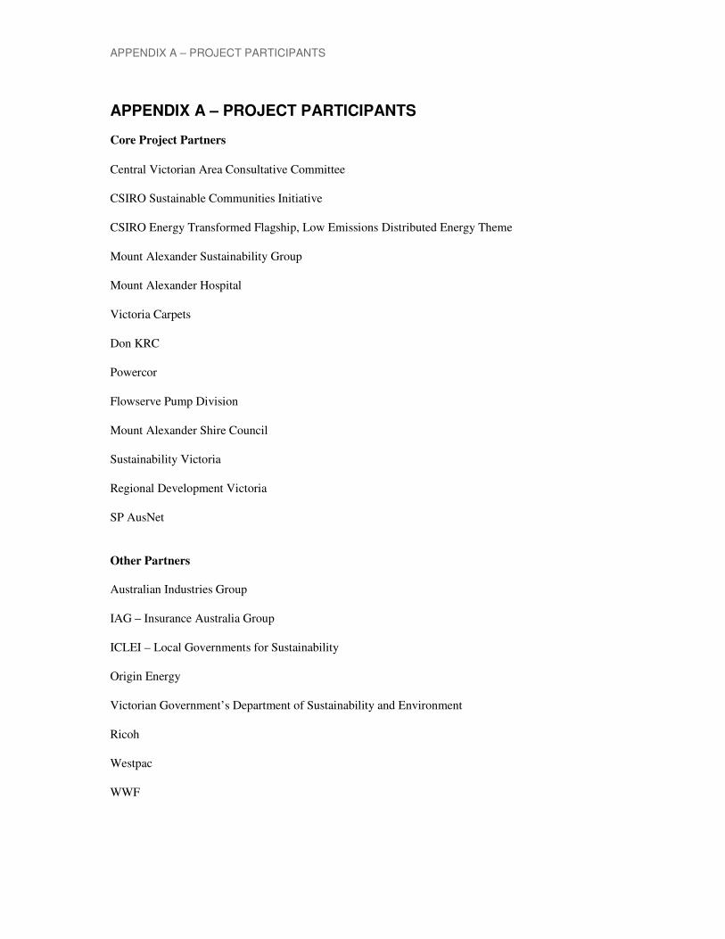
APPENDIX A – PROJECT PARTICIPANTS
APPENDIX A – PROJECT PARTICIPANTS
Core Project Partners
Central Victorian Area Consultative Committee
CSIRO Sustainable Communities Initiative
CSIRO Energy Transformed Flagship, Low Emissions Distributed Energy Theme
Mount Alexander Sustainability Group
Mount Alexander Hospital
Victoria Carpets
Don KRC
Powercor
Flowserve Pump Division
Mount Alexander Shire Council
Sustainability Victoria
Regional Development Victoria
SP AusNet
Other Partners
Australian Industries Group
IAG – Insurance Australia Group
ICLEI – Local Governments for Sustainability
Origin Energy
Victorian Government’s Department of Sustainability and Environment
Ricoh
Westpac
WWF

APPENDIX B – CALCULATION PROCEDURES
61
APPENDIX B – CALCULATION PROCEDURES
Solar Photovoltaic
The performance of a solar photovoltaic (PV) installation can be derived using Steps 1-2.
Calculations are performed for each hour of the data set (preferably a year or more long) to
calculate the electrical output and greenhouse gas savings for a 1 kW PV panel. Savings for a
larger system are simply scaled to the appropriate size by multiplying the outputs by the number
of units installed.
Step 1: For each hour calculate the electrical output from a nominal 1 kW array. A panel is
assumed to produce 1 kW for a shortwave radiative flux of 1000 W/m2 at an ambient
temperature of 25°C. A temperature correction loss factor of 0.4% per degree increase in
ambient temperature is applied:
25)-(ATPTT
T/100),(0.4-1 LF
LFRkWh in
+∆=∆
∆=
=
Step 2: Calculate the greenhouse gas savings for a year:
HPY
i
i 1
GHG (kWh GridER)=
= ∑
Step 3: Calculate the energy costs:
[ ]
[ ] [ ]
[ ]
[ ]
PVbase
grid
iiHPM1,i
gridgridPV
grid
iHPM1,igridgridbase
HPY
1i
i
ECEC∆EC
,NU(kWh)REC
)HPM
αDC)NU(kWh-EL(max
)NCUCαNU(kWh)-EL(EC
),HPM
DCBoilEffEL(max)NCUC(ELEC
)(EC EC
−=
−
++=
++=
=
=
=
=
∑

APPENDIX B – CALCULATION PROCEDURES
Where,
kWh is the electrical output for a 1 kW unit (kWh)
Rin is the hourly average short wave radiation flux over one square metre (kW/m2)
LF is the temperature loss factor
∆T is the temperature differential between the panel and air normalised to 25°C (°C)
∆PT is the panel operating temperature above ambient (°C)
AT is the ambient temperature (°C)
GHG is the greenhouse gas savings from a solar panel per year (kg/y)
GridER is the emission factor for grid based electricity (kg/kWh)
EL is the electrical requirement of the business (kWh)
α is a scalar equal to 1 when importing and set a value determined a feed-in tariff when
exporting
EC is the annual difference in energy cost for a solar PV installation ($/y)
ECbase is the cost of energy supply for the current system ($/h)
ECPV is the cost of energy supply for the solar PV unit ($/h)
∆EC is the hourly difference in energy cost for a solar PV installation ($/h)
UCgrid is the usage charge for grid electricity for the given hour ($/kWh)
NCgrid is the network charge for grid electricity for the given hour ($/kWh)
DCgrid is the demand charge for grid electricity ($/kW) based on the peak demand (kW) for the
given month
REC is the income from renewable energy certificates ($/kWh)
HPM are the number of hours in the given month
HPY are the number of hours in the given year.
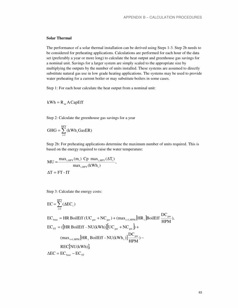
APPENDIX B – CALCULATION PROCEDURES
63
Solar Thermal
The performance of a solar thermal installation can be derived using Steps 1-3. Step 2b needs to
be considered for preheating applications. Calculations are performed for each hour of the data
set (preferably a year or more long) to calculate the heat output and greenhouse gas savings for
a nominal unit. Savings for a larger system are simply scaled to the appropriate size by
multiplying the outputs by the number of units installed. These systems are assumed to directly
substitute natural gas use in low grade heating applications. The systems may be used to provide
water preheating for a current boiler or may substitute boilers in some cases.
Step 1: For each hour calculate the heat output from a nominal unit:
CapEffARkWh in=
Step 2: Calculate the greenhouse gas savings for a year
GasER)(kWh GHGHPY
1i
i∑=
=
Step 2b: For preheating applications determine the maximum number of units required. This is
based on the energy required to raise the water temperature:
IT-FTT
,)(kWhmax
)T(maxCp)m(max MU
iHPYi,
iHPYi,iHPYi,
=∆
∆=
Step 3: Calculate the energy costs:
[ ]
[ ][ ]
[ ]
[ ]
STbase
gas
iiHPM1,i
gasgasST
gas
iHPM1,igasgasbase
HPY
1i
i
ECEC∆EC
,NU(kWh)REC
)HPM
DC)NU(kWh-BoilEffHR(max
)NCUCNU(kWh)-BoilEffHR(EC
),HPM
DCBoilEffHR(max)NCUC(BoilEffHREC
)EC( EC
−=
−
++=
++=
∆=
=
=
=
∑

APPENDIX B – CALCULATION PROCEDURES
Where,
kWh is the heat output for a nominal unit (kWh)
Rin is the hourly average short wave radiation flux over one square metre (kW/m2)
A is the capture area (m2)
CapEff is the efficiency rate of capture (%, expressed in decimal form)
GHG is the greenhouse gas savings from a solar panel per year (kg/y)
HPY is the number of hours per year
GasER is the emission factor for natural gas (kg/kWh)
MU is the maximum number of units required for preheating water
m is the mass of water to be heated (kg)
Cp is the heat capacity of water (kWh/kg °C)
FT is the final temperature of the water being heated (°C)
IT is the initial temperature of the water to be heated (°C)
∆T is the temperature difference between the initial and final states
NU is the number of units to be installed
HR is the heat requirement (kWh)
BoilEff is the efficiency of a boiler (%, expressed in decimal form)
EC is the annual difference in energy cost for a solar thermal installation ($/y)
ECbase is the cost of energy supply for the current system ($/h)
ECST is the cost of energy supply for the solar thermal unit ($/h)
∆EC is the hourly difference in energy cost between the base and CHP cases ($/h)
UCgas is the usage charge for natural gas supply for the given hour ($/kWh)
NCgas is the network charge for natural gas supply for the given hour ($/kWh)
DCgas is the demand charge for natural gas supply ($/kW) based on the peak demand (kW) for
the given month
REC is the income from renewable energy certificates ($/kWh)

APPENDIX B – CALCULATION PROCEDURES
65
HPM are the number of hours in the given month
HPY are the number of hours in the given year.
Note: 1 GJ = 277.78 kWh

APPENDIX B – CALCULATION PROCEDURES
Wind
The performance of a wind turbine installation can be derived using Steps 1-3. Calculations are
performed for each hour of the data set (preferably a year or more long) to calculate the
electrical output and greenhouse gas savings for a nominal wind turbine. Savings for a larger
system are simply scaled to the appropriate size by multiplying the outputs by the number of
units installed.
Step 1: For each hour calculate the electrical output from a nominal wind turbine from the
atmospheric wind speed at the required height:
)U(fkWh =
If wind speed data are only available at 10 m height (the standard for meteorological stations)
then the speed at higher locations can be derived from the following:
γ
=10h
h10UU
Step 2: Calculate the greenhouse gas savings for a year:
GridER)(kWh GHGHPY
1i
i∑=
=
Step 3: Calculate the energy costs:
[ ]
[ ] [ ]
[ ]
[ ]
WTbase
grid
HPM1,i
gridgridWT
grid
HPM1,igridgridbase
HPY
1i
ECEC∆EC
,NU(kWh)REC
)HPM
αDCNU(kWh)-EL(max
)NCUCαNU(kWh)-EL(EC
),HPM
DCBoilEffEL(max)NCUC(ELEC
∆EC EC
−=
−
++=
++=
=
=
=
=
∑

APPENDIX B – CALCULATION PROCEDURES
67
Where,
kWh is the electrical output for a nominal unit (kWh)
U is the hourly average wind speed (m/s) at the required height (h)
f( U ) is the functional form of the turbine output (kWh)
h is the height of the wind turbine (m)
h10 is a height of 10m
γ is an exponential whose value is determined by the land use and atmospheric conditions
GHG is the greenhouse gas savings from a solar panel per year (kg/y)
GridER is the emission factor for grid based electricity (kg/kWh)
EL is the electrical requirement of the business (kWh)
α is a scalar equal to 1 when importing and set a value determined by negotiations with a
retailer or potentially a feed-in tariff if applicable when exporting
EC is the annual difference in energy cost for a wind turbine installation ($/y)
ECbase is the cost of energy supply for the current system ($/h)
ECWT is the cost of energy supply for the wind turbine ($/h)
∆EC is the hourly difference in energy cost between the base and CHP cases ($/h)
UCgrid is the usage charge for grid electricity for the given hour ($/kWh)
NCgrid is the network charge for grid electricity for the given hour ($/kWh)
DCgrid is the demand charge for grid electricity ($/kW) based on the peak demand (kW) for the
given month
REC is the income from renewable energy certificates ($/kWh)
HPM are the number of hours in the given month
HPY are the number of hours in the given year

APPENDIX B – CALCULATION PROCEDURES
CHP (Dual Stream)
The total system performance for a dual stream CHP option can be derived using Steps 1-4.
Calculations are performed for each hour of the data set (preferably a year or more long) to
calculate the system requirement, the system outputs, supplementary boiling and electricity
loads, greenhouse gas emissions and operation costs.
Step 1: For each hour calculate engine capacity to match the maximum of electrical or heat
load:
engine
engine
engine
jacket
jacket
exhaust
exhaust ElecEff/ElecEff
ER,
CapEff
HR,
CapEff
HRmaxGL
=
Step 2: Calculate the actual generation and supplementary boiling and electricity requirements:
[ ]
),HR -HLmax(0, L
),HR-HLmax(0, L
,ER-ElecGen L
,CapEffElecEff
ElecGen HL
,CapEffElecEff
ElecGen HL
,EngineCapGL,minElecGen
exhaustexhaustexhaust
jacketjacketjacket
engine engine
exhaust
engine
exhaust
jacket
engine
jacket
=∆
=∆
=∆
=
=
=
Step 3: Calculate the greenhouse gas emissions from the system:
[ ][ ]
engine
engine
CHPbase
engineexhaustjacketengineCHP
exhaustjacketenginebase
HPY
1i
i
ElecEff
ElecGenGC
,GHGGHGGHG
),GridERL()GasERLL()GasERGC(GHG
),GasERBoilEffHRHR()GridERER(GHG
)GHG( GHG
=
−=∆
∆+∆+∆+=
++=
∆=∑=

APPENDIX B – CALCULATION PROCEDURES
69
Step 4: Calculate the energy costs:
[ ]
[ ] [ ]
[ ]
[ ]
[ ]
[ ]
CHPbase
gas
exhaustjacketengineHPM1,i
gasgasexhaustjacketengine
grid
engine
HPM
1igridgridengineCHP
gas
exhaustjacketHPM1,i
gasgasexhaustjacket
grid
engineHPM1,igridgridenginebase
HPY
1i
i
ECEC∆EC
),HPM
DCBoilEff)HRHR(GC(max
))NCUC(BoilEffLL((GC
)HPM
αDCL(max)NCUCαL(EC
),HPM
DCBoilEffHRHR(max
)NCUCBoilEffHRHR(
)HPM
DCER(max)NCUC(EREC
)EC( EC
iii
ii
i
−=
++
++∆+∆+
+∆++∆=
+
+++
+++=
∆=
=
=
=
=
=
∑

APPENDIX B – CALCULATION PROCEDURES
Where,
GL is the maximum electrical output of the generator (kWh)
HRjacket is the heat requirement from the jacket water (kWh)
HRexhaust is the heat requirement from the jacket water (kWh)
ERengine = EL is the electrical requirement (kWh)
CapEff jacket is the capture efficiency of the jacket waste stream (%, expressed in decimal form)
CapEff exhaust is the capture efficiency of the exhaust waste stream (%, expressed in decimal
form)
ElecEffengine is the electrical efficiency of the CHP unit (%, expressed in decimal form)
ElecGen is the actual generation by the unit (kWh)
EngineCap is the maximum electrical output of the generator (kWh)
HLjacket is the heat output of the jacket water (kWh)
HLexhaust is the heat output of the exhaust stream (kWh)
∆Lengine is the difference between actual and required electrical load (kWh)
∆Ljacket is the difference between actual and required jacket heat load, negative values represent
wasted heat (kWh)
∆Lexhaust is the difference between actual and required exhaust heat load, negative values
represent wasted heat (kWh)
BoilEff is the efficiency of a boiler (%, expressed in decimal form)
GHG is the annual greenhouse gas savings from a CHP installation (kg/y)
GHGbase are the greenhouse gas emissions for the current system (kg/h)
GHGCHP are the greenhouse gas emissions for the CHP unit (kg/h)
∆GHG is the difference in greenhouse gas emissions between the base and CHP cases (kg/h)
GasER is the emission rate for gas (kg/kWh)
GridER is the emission rate for grid based electricity (kg/kWh)
GCengine is the gas consumption rate for the engine (kWh)
EC is the annual difference in energy cost for a CHP plant ($/y)

APPENDIX B – CALCULATION PROCEDURES
71
ECbase is the cost of energy supply for the current system ($/h)
ECCHP is the cost of energy supply for the CHP unit ($/h)
∆EC is the difference in energy cost between the base and CHP cases ($/h)
α is a scalar equal to 1 when importing and set a value determined by negotiations with a
retailer when exporting
UCgrid is the usage charge for grid electricity for the given hour ($/kWh)
NCgrid is the network charge for grid electricity for the given hour ($/kWh)
DCgrid is the demand charge for grid electricity ($/kW) based on the peak demand (kW) for the
given month
UCgas is the usage charge for natural gas supply for the given hour ($/kWh)
NCgas is the network charge for natural gas supply for the given hour ($/kWh)
DCgas is the demand charge for natural gas supply ($/kW) based on the peak demand (kW) for
the given month
HPM are the number of hours in the given month
HPY are the number of hours in the given year.
Note: 1 GJ = 277.78 kWh

APPENDIX B – CALCULATION PROCEDURES
Economics
Net Present Value
Net present value (NPV) is a measure of the profitability of a project. It is the difference
between the present value of cash inflows and the present value of cash outflows over the life of
the project. It is considered an absolute measure of project merit. A key factor in the NPV
calculation is the rate used to discount future cash flows to their present value. It is calculated
by the following formula:
( )∑
=
−
+=
T
1i
0i Cr1
C NPV
i
Where,
NPV is the net present value ($)
T is the number of years
r is the discount rate (%, expressed in decimal form)
C is the net cash flow, where C0 represents the initial capital investment.
Internal Rate of Return
The internal rate of return (IRR), sometimes referred to as the economic rate of return, is a
common metric used to gauge the viability of an investment. It is an indicator of the quality of
an investment (compared to NPV which provides a value or magnitude).Generally speaking, the
higher the IRR the more desirable it is to undertake the project.
An iterative solver is employed to find the value of the discount rate (r) which satisfies the
following equation:
( )∑
=
=
−
+=
T
1i
0i 0Cr1
C NPV
i
Where,
IRR is the internal rate of return which corresponds to the discount rate (r) when this function is
zero
T is the number of years
r is the discount rate (%, expressed in decimal form)
C is the net cash flow, where C0 represents the initial capital investment.

APPENDIX B – CALCULATION PROCEDURES
73
Simple Payback
Companies frequently require that the upfront capital outlay of any project be recoverable
within some specified period of time. This is defined as the payback period. Some consider just
a ‘simple payback’ where no discount rate is applied. The simple payback period is calculated
as the upfront capital cost divided by the annual savings.
The payback method mainly indicates a project’s liquidity rather than its profitability. It is used
as a measure of a project’s riskiness, since liquidity deals with how fast an investment can be
recovered. A low-valued payback period is considered desirable.
It is calculated by the following formula:
AS
CSP 0=
Where,
SP is the payback time (years)
C0 is the capital investment ($)
AS are the annual savings ($).
Discounted Payback
Alternatively, a ‘discounted payback’ recognises the time value of money and estimates the
number of years required to recover the original investment discounted by the cost of the
project. It takes into account a time value on investment (discount rate). It allows an estimate of
present value taking into account future accrual. An iterative solver is used to find the number
of years which satisfies the following equation:
( )∑
=
=
−
+=
T
1i
0i
i 0Cr1
AS DP
Where,
DP is the payback time (years)
r is the discount rate (%, expressed in decimal form)
AS are the annual savings ($)
T is the upper bound on the number of years.

APPENDIX C – GLOSSARY
APPENDIX C – GLOSSARY
Acronym Description AC Alternating Current
AEMC Australian Energy Market Commission AER Australian Energy Regulator
AMG Asynchronous machine CHP Combined Heat and Power
CO2e Carbon dioxide equivalent
CPRS Carbon Pollution Reduction Scheme CSIRO Commonwealth Scientific and Industrial Research Organisation
DC Direct Current DLF Distribution Loss Factor
DMIA Demand Management Incentive Allowance DMIS Demand Management Incentive Scheme
DNSP Distribution Network Service Provider
DUoS Distribution Use of System charge ESCO Energy Services Company
ESCV Essential Services Commission Victoria HV High Voltage
HVAC Heating Ventilation and Air Conditioning IPART Independent Pricing and Regulatory Tribunal
LV Low Voltage
MASG Mount Alexander Sustainability Group MCE Ministerial Council on Energy
MLF Marginal Loss Factor MV Medium Voltage
NEM National Electricity Market NEMMCO National Electricity Market Management Company
NER National Electricity Rules
Ofgem Office of the Gas and Electricity Markets (UK) OTN Obligation Transfer Number
PV Photovoltaic RDV Regional Development Victoria
REAP Regional Electric Access Program REC Renewable Energy Certificate
SCI Sustainable Communities Initiative
SV Sustainability Victoria TLF Transmission Loss Factor
TNSP Transmission Network Service Provider TUoS Transmission Use of System charge

APPENDIX D – ENERGY EFFICIENCY AUDIT SUMMARY
75
APPENDIX D – ENERGY EFFICIENCY AUDIT SUMMARY
In this Appendix brief details from external energy audits are provided. It should be noted when considering the totals that the savings are compared to the baseline total and that adoption of certain options like power factor correction for instances would affect the values of other options implemented afterwards. It should also be noted that the GHG savings have been adjusted to match the emission rates for avoided electricity and gas adopted in this report (see Section 2.2) as the estimates from the auditors have ignored transmission and distribution savings.
Site 1 Site 1 is a large and varied business which has many potential energy savings possibilities. The largest single saving is from the potential use of cogeneration. The figures in Table D1are updates based on a specific addition of 4MW unit (2x2MW with supplemental gas boilers) for a proposed expanded facility. The savings in this case from the cogeneration would be around 39 % of their projected total emissions based on average consumption patterns if all of the heat converted to steam and hot water is utilised. If only a portion of the total heat recovered is used (say 60% representing all of the steam and part of the hot water) then the total efficiency will be somewhat lower, around 35% for this assumption. The recommendations in Table D1 are six options provided by an external energy and water audit that the business considers as potential candidates for their business
Table D1. Potential greenhouse savings provided by an external audit in 2009.
Project Energy Saving
(kWh / GJ)
Cost Saving
($)
GHG Saving (tCO2e)
Project Cost ($)
Simple Payback (years)
Cogeneration (4MW) 25,792,000 kWh and
-125,105 GJ
2,080,000 32,380 8,600,000 4.1
Xflame panel 154,500 kWh 17,000 237 663,500 39 Rainwater harvesting/reuse 35,994 575,900 16
Refrigeration heat recovery 420,500 kWh 64,000 644 240,000 3.8
Occupancy sensing offices 18,180 kWh 2,000 28 20,000 10 P6 office daylighting 81,820 kWh 9,000 125 78,000 8.7
Total 2,207,994 33,661 10,177,400
Site 2 Table D2 provides an indication of potential greenhouse savings from a recent external audit of the Site 2 business. For comparison Table D3 provides an indication of greenhouse savings from an earlier audit as part of the federal government greenhouse challenge in 1998. Discussions with site staff indicate that the business processes have changed little since the earlier report and it is interesting to note a difference in potential energy savings of around a factor of 3 to 4 (ignoring the cogeneration option). This highlights the variation that can be attributed to different audit processes. It also highlights that there are many potential energy savings measures and that to properly evaluate them takes a combination of external and internal skills. In both cases the simple paybacks for most options are within 3 to 4 years.
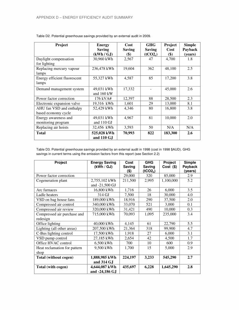
APPENDIX D – ENERGY EFFICIENCY AUDIT SUMMARY
Table D2. Potential greenhouse savings provided by an external audit in 2009.
Project Energy Saving
(kWh / GJ)
Cost Saving
($)
GHG Saving (tCO2e)
Project Cost ($)
Simple Payback (years)
Daylight compensation for lighting
30,960 kWh 2,567 47 4,700 1.8
Replacing mercury vapour lamps
236,478 kWh 19,604 362 48,100 2.5
Energy efficient fluorescent lamps
55,327 kWh 4,587 85 17,200 3.8
Demand management system 49,031 kWh and 160 kW
17,332 - 45,000 2.6
Power factor correction 176 kVA# 12,397 88 28,500 2.3
Electronic expansion valve 19,316 kWh 1,601 29 13,000 8.1
AHU fan VSD and enthalpy based economy cycle
52,429 kWh 4,346 80 16,800 3.8
Energy awareness and monitoring program
49,031 kWh and 110 GJ
4,967 81 10,000 2.0
Replacing air hoists 32,456 kWh 3,593 50 N/A N/A
Total 525,028 kWh and 110 GJ
70,993 822 183,300 2.6
Table D3. Potential greenhouse savings provided by an external audit in 1998 (cost in 1998 $AUD). GHG
savings in current terms using the emission factors from this report (see Section 2.2)
Project Energy Saving (kWh / GJ)
Cost Saving
($)
GHG Saving (tCO2e)
Project Cost ($)
Simple Payback (years)
Power factor correction 29,000 320 85,000 2.9
Cogeneration plant 2,755,102 kWh and -21,500 GJ
211,500 2,995 1,100,000 5.2
Arc furnaces 16,800 kWh 1,716 26 6,000 3.5
Ladle heaters 314 GJ 7,500 18 30,000 4.0
VSD on bag house fans 189,000 kWh 18,916 290 37,500 2.0 Compressed air control 340,000 kWh 33,070 521 3,000 0.1
Compressed air review 320,000 kWh 31,421 490 10,000 0.3 Compressed air purchase and redesign
715,000 kWh 70,093 1,095 235,000 3.4
Office lighting 40,000 kWh 4,145 61 22,790 5.5
Lighting (all other areas) 207,500 kWh 21,364 318 99,900 4.7
C-Bus lighting control 17,500 kWh 1,918 27 6,000 3.1
VSD pump control 27,185 kWh 2,654 42 4,500 1.7
Office HVAC control 6,500 kWh 700 10 600 0.9
Heat reclamation for pattern shop
9,500 kWh 1,700 15 5,000 2.9
Total (without cogen) 1,888,985 kWh and 314 GJ
224,197 3,233 545,290 2.7
Total (with cogen) 4,644,087 kWh and -24,186 GJ
435,697 6,228 1,645,290 2.8
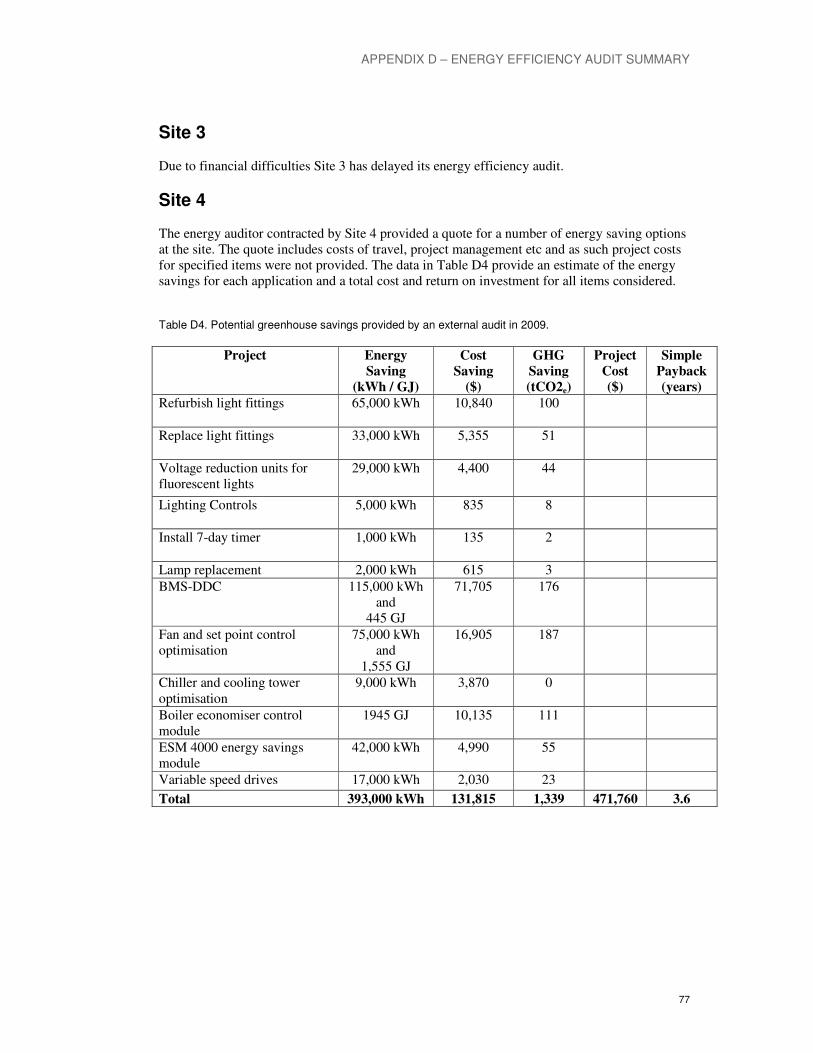
APPENDIX D – ENERGY EFFICIENCY AUDIT SUMMARY
77
Site 3 Due to financial difficulties Site 3 has delayed its energy efficiency audit.
Site 4 The energy auditor contracted by Site 4 provided a quote for a number of energy saving options at the site. The quote includes costs of travel, project management etc and as such project costs for specified items were not provided. The data in Table D4 provide an estimate of the energy savings for each application and a total cost and return on investment for all items considered.
Table D4. Potential greenhouse savings provided by an external audit in 2009.
Project Energy Saving
(kWh / GJ)
Cost Saving
($)
GHG Saving (tCO2e)
Project Cost ($)
Simple Payback (years)
Refurbish light fittings 65,000 kWh 10,840 100
Replace light fittings 33,000 kWh 5,355 51
Voltage reduction units for fluorescent lights
29,000 kWh 4,400 44
Lighting Controls 5,000 kWh 835 8
Install 7-day timer 1,000 kWh 135 2
Lamp replacement 2,000 kWh 615 3
BMS-DDC 115,000 kWh and
445 GJ
71,705 176
Fan and set point control optimisation
75,000 kWh and
1,555 GJ
16,905 187
Chiller and cooling tower optimisation
9,000 kWh 3,870 0
Boiler economiser control module
1945 GJ 10,135 111
ESM 4000 energy savings module
42,000 kWh 4,990 55
Variable speed drives 17,000 kWh 2,030 23
Total 393,000 kWh 131,815 1,339 471,760 3.6
