maintenance optimisation for wind turbines … · for wind turbines jesse agwandas ... 5.2.3...
TRANSCRIPT

MAINTENANCE OPTIMISATION FOR WIND TURBINES
JESSE AGWANDAS ANDRAWUS
A thesis submitted in partial fulfilment of the requirements of
The Robert Gordon University for the degree of Doctor of Philosophy
April 2008

Maintenance Optimisation for Wind Turbines
PhD Thesis, The Robert Gordon University Aberdeen, 2008. I
SUPERVISORS AND FUNDING
Principal Supervisor: Professor John F Watson BSc, PhD Second Supervisor: Dr Mohammed Kishk BSc, MSc, PhD
Funding: The Robert Gordon University

Maintenance Optimisation for Wind Turbines
PhD Thesis, The Robert Gordon University Aberdeen, 2008. II
CONTENTS PAGE LIST OF FIGURES………………………………………………………………VIII LIST OF TABLES……………………………………………………………...….XI ACKNOWLEDGEMENTS………………………………...…………………….XIII DEDICATION…..…………..……………………………………………………XIV ABSTRACT……………………………………………………………………….XV 1 INTRODUCTION..…………… …………………………..……………….1 1.1 Background..……………………………………………………..…..1 1.2 Renewable Energy..……………………………………………..…...2 1.3 Wind Energy Generation..………………………………………..….2 1.4 Challenges of Investment in the Wind Energy Industry…………......3 1.5 Common Maintenance Strategies Applied to Wind Turbines..…..….3 1.5.1 Preventative Maintenance………………………………...….4 1.5.2 Corrective Maintenance..……………………………..……...5 1.6 Problems Associated with the Current Maintenance Practises of Wind Turbines..……………………………………..……………………...5
1.7 Asset Management…………………………………...……………....7 1.7.1 Asset Management in other industrial sectors…………….....8
1.7.1.1 The Oil and Gas Sector……………………..……......8 1.7.1.2 Electricity Supply Industry…..……………………....8 1.7.1.3 Water Supply Industry……………..…………….......9 1.7.1.4 Transport Services……………..………………….....9
1.7.2 Processes of Asset Management……………...……………...9 1.8 Asset Management and the Wind Energy Industry..………..……...10 1.9 Tools and Techniques of Asset Management..…………..…………11 1.9.1 Reliability Centred Maintenance..…………..……………...12
1.10 Condition Based Maintenance Strategy.....……………………...….12 1.11 Maintenance Optimisation.………………………………................13 1.11.1 Benefits of Maintenance Optimisation for wind turbines…..14
1.12 Research Aim and objectives.…………………………………...….15 1.12.1 Research aim.…………………………………...…………..15 1.12.2 Research objectives.………………………………...………15 1.13 Thesis layout..…………………………………………………..…..15

Maintenance Optimisation for Wind Turbines
PhD Thesis, The Robert Gordon University Aberdeen, 2008. III
2 LITERATURE REVIEW ..………………………………….…….……...18
2.1 Introduction.……………………………………………...…….…...18 2.2 The Wind Energy Industry.…………………………….…..…….…18
2.2.1 Onshore and Offshore wind energy generation.....................18 2.3 Wind Turbines..………………………………………………..…...19
2.3.1 Design Types…………………………………………….....20 2.3.2 Components Functionality, Design Materials and Failure
characteristics..........................................................………...23 2.3.2.1 Blades…………………………..…………………...23 2.3.2.2 Causes of fibreglass reinforced plastic blades
failure.........................................................................25 2.3.2.3 Hub………………..………………………………...25 2.3.2.4 Main Shaft…………………..……………………....26 2.3.2.5 Main Bearing………………………………..……...26 2.3.2.6 Causes of main bearing failures.................................26 2.3.2.7 Gearbox……………………………………..……....26 2.3.2.8 Causes of gearbox failures.........................................28 2.3.2.9 Generator……………………………..……….........28 2.3.2.10 Causes of squirrel cage induction generator
failures.......................................................................29 2.3.2.11 Blade Pitching System…………………………....29 2.3.2.12 Causes of blade pitching failures............................30 2.3.2.13 Mechanical Brake………………….........……..…30 2.3.2.14 Causes of Mechanical brake failures......................30 2.3.2.15 Hydraulic System………………………………....31 2.3.2.16 Causes of hydraulic system failures........................31 2.3.2.17 Yaw Drive…………………………………...…....31 2.3.2.18 Causes of yaw system failures................................32 2.3.2.19 Electronic Controller……………………………..32 2.3.2.20 Nacelle, Canopies and Spinners…………….…....33 2.3.2.21 Tower……………………………………...…..….34 2.3.2.22 Foundation………………………………...……...34
2.4 Cost significant items in a Wind Turbine…………………………..34 2.5 Tools and Techniques of Asset Management…………………........35
2.5.1.1 Hazard and Operability Study…………………....…36 2.5.1.2 Fault Tree Analysis…………………………………36 2.5.1.3 Event Tree Analysis………………………………...36 2.5.1.4 Critical Task Analysis………………………………37 2.5.1.5 Quantified Risk Analysis…………………………...37 2.5.1.6 Root Cause Analysis……………………….…...…..37 2.5.1.7 Structured What-if Technique……………….…...…37
2.6 Condition Monitoring Techniques and Wind Turbines………….....38 2.6.1 Strain Measurement……………………........……...38 2.6.2 Acoustic Analysis Technique………………………38 2.6.3 Vibration Analysis Technique……………………...39 2.6.4 Performance/Process Parameter Technique…….…..39 2.6.5 Visual Examination…………………………………40

Maintenance Optimisation for Wind Turbines
PhD Thesis, The Robert Gordon University Aberdeen, 2008. IV
2.6.6 Fibre Optics Measurement………………………….40 2.6.7 Oil Analysis Technique……………………………..41
3 APPROACH AND METHODOLOGY…………………… …………….42
3.1 Introduction…………………………………………………………42 3.2 Design of a structured asset management model…………………...42 3.3 Selection of a suitable Maintenance Strategy………………………44
3.3.1 Total Productive Maintenance……………………………...44 3.3.2 Risk Based Inspection………………………………………44 3.3.3 Reliability Centred Maintenance…………………………...45 3.3.4 A Hybrid Approach (RCM plus ALCA)…………………...46
3.4 Maintenance Optimisation………………………………………….47 3.4.1 Types of Maintenance Optimisation………………………..48
3.4.1.1 Quantitative Maintenance Optimisation…………...48 3.5 Modelling System Failures…………………………………………49
3.5.1 Statistical Distributions……………………………………..49 3.5.2 Weibull Distribution……………………………...………...50 3.5.3 Parameter Estimation Techniques………………...………..51 3.5.4 Maximum Likelihood Estimation…………………...……...52
3.6 Delay-Time Maintenance Mathematical Model……………………54 3.6.1 Concept of the delay-time mathematical model……………55 3.7 Data Requirement and Collection…………………………………..57 3.6 Summary……………………………………………………………57
4 A STRUCTURED MODEL FOR ASSET MANAGEMENT IN THE
WIND ENERGY INDUSTRY……………………… ……………………59
4.1 Introduction…………………………………………………………59 4.2 Asset Management Processes in the Wind Energy Industry……….59 4.3 Detail Design of the Model………………………………………....60
4.3.1 Stakeholders’ Requirements………………………………..60 4.3.2 Mission and Vision Statements……………………………..61 4.3.3 Asset Classification..………………………………….…….62 4.3.4 Primary Asset……………………………………………….63 4.3.5 Secondary Assets…………………………………………...64
4.3.5.1 Data…………………………………………………64 4.3.5.2 Work force………………………………………….66
4.3.6 The Overall Continuous Performance Improvement……….66 4.4 The Overall Picture…………………………………………………67 4.5 The benefits of the system………………………………………….67 4.6 Practical Implementation…………………………………………...69
4.6.1 Institutional Barriers………………………………………..69 4.6.2 Responsibilities……………………………………………..70
4.7 Summary……………………………………………………………71

Maintenance Optimisation for Wind Turbines
PhD Thesis, The Robert Gordon University Aberdeen, 2008. V
5 SELECTION OF A SUITABLE MAINTENACE STRATEGY FOR WIND TURBINES…………… …………………………………………...72 5.1 Introduction…………………………………………………………72 5.2 Application of RCM to a Generic Horizontal Axis Wind Turbine…72
5.2.1 Function and Performance Standards of a Wind Turbine…..73 5.2.2 Functional Failures………………………………………….73 5.2.3 Failure Modes and Effect Analysis…………………………73
5.3 A Case Study………………………………………………………..73 5.3.1 Data Collection...……………………………………...……75 5.3.2 Failure Consequences………….………………………...…75 5.3.3 Selection of CBM Tasks……………………………………78 5.3.4 Economic Analysis of CBM and Comparison with TBM….81 5.3.5 Uncertainties and Risk Assessment………………………...82 5.3.6 Evaluation of Non-financial Factors………………………..86 5.3.7 Benefit-To-Cost Ration Evaluation………………………...88 5.3.8 Effect of Failure Rates……………………………………...89
5.4 Summary……………………………………………………………89
6 ASSESSMENT OF WIND TURBINES FIELD FAILURE DATA... .....91 6.1 Introduction…………………………………………..….………....91 6.2 Data Collection………………………………………………..…....91 6.3 Shape and Scale Parameters of components and subsystems of 600
kW Wind Turbines……………....……………...........................….95 6.3.1 Main Shaft.....................................…..…………………......96 6.3.2 Main Bearing………………................………..…………...98 6.3.3 Gearbox………………………........................…...………...99 6.3.4 Generator....................……………………...……………...101
6.4 A Case Study………………………………………………...…….103 6.4.1 Reliability Trend of critical components of the 600 kW
Turbine………………………………………...…………..103 6.4.2 Maintenance Optimisation…………………………...…....104 6.4.3 Optimisation of Time-Based Maintenance Tasks………....105
6.4.3.1 Gearwheels...............................................................106 6.4.3.2 Intermediary speed shaft bearings...........................107 6.4.3.3 Main shaft................................................................108 6.4.3.4 Main bearings...........................................................109 6.4.3.5 Gearbox HSS bearings.............................................110 6.4.3.6 Generator bearings...................................................111
6.5 Summary………………………………………………………..…112 7 MODELLING WIND TURBINE FAILURES TO OPTIMISE
MAINTENANCE………… …………………………………...………....114 7.1 Introduction……………………………………………………......114
7.2 Modelling Failures of the 600 kW Wind Turbine………………...114 7.3 600 kW Wind Turbine Model Assessment………………………..117

Maintenance Optimisation for Wind Turbines
PhD Thesis, The Robert Gordon University Aberdeen, 2008. VI
7.4 Wind Farm Model Assessment……………………………………120 7.5 Reliability, Availability and Maintainability Optimisation……….124 7.5.1 The Wind Turbine…………………………………………124 7.5.2 The Wind Farm……………………………………………126 7.6 Summary…………………………………………………………..129
8 THE DELAY-TIME APPROACH TO MAINTENANCE
OPTIMISATION…………… ……………………………………….......131 8.1 Introduction…………………………………………………...…...131
8.2 A Case Study……………………………………………………....131 8.2.1 Failure Mode and Effect Criticality Analysis………….….131 8.2.2 Vibration Analysis…………………………………….......132 8.2.3 Failure Consequences of Subsystems………………….….133 8.2.4 Cost of Inspection and Repair of Components…….……...134 8.2.5 Defects Rate………………………………………….........135 8.2.6 Delay-Time………………………………………………..136
8.3 Summary…………………………………………………………..138
9 COMPARATIVE STUDIES…………………… ……………………….140 9.1 Introduction………………………………………………………..140 9.2 Overview result of the Modelling System Failures technique…….140 9.3 Overview result of the Delay-time Model…….………………......141 9.4 Comparison of MSF and DTMM...…………………………...…..142 9.4.1 Practical Implementation…………………………..….…..142 9.4.2 Potential Benefits…………………………………...……..142 9.5 Summary…………………………………………………..….…...143 10 SUMMARY, CONCLUSIONS AND RECOMMENDATIONS…… ...145 10.1 Summary…………………………………………………………..145 10.1.1 A structured model for AM in the wind industry…………145 10.1.2 Suitable maintenance strategies for wind turbines………..147 10.1.3 Optimised maintenance of wind turbines…………………149 10.2 Conclusions………………………………………………………..153 10.3 Recommendations for further research……………………………154 10.3.1 Modelling Wind Turbine Failures…………………….......154 10.3.2 Development of novel Web-based software……………....155 11 REFERENCES…………………………………………………………...157 APPENDIX A……………………………………………………………….……167
A1…………………………………………………………………….……167
A2………………………………………………………………………….180

Maintenance Optimisation for Wind Turbines
PhD Thesis, The Robert Gordon University Aberdeen, 2008. VII
A3……………………………………………………………….......…….184
APPENDIX B: GLOSSARY.................................................................................189
APPENDIX C: ABSTRACTS OF PUBLISHED PAPERS...............................191

Maintenance Optimisation for Wind Turbines
PhD Thesis, The Robert Gordon University Aberdeen, 2008. VIII
LIST OF FIGURES FIGURE PAGE
Figure 1.1 Generic Business Model showing key Issues..............................................10
Figure 2.1 Components and Subsystems of a typical HAWT wind turbine…...21
Figure 2.2 Causes of wind turbine failures- The German experience………….22
Figure 2.3 Wind turbine component failures in the UK………………………..23
Figure 2.4 Causes of offshore wind turbines failure in the Netherlands….……23
Figure 2.5 Components of a 3-stage planetary gearbox………………………..28
Figure 2.6 Cost significant items of a typical wind turbine…………………....35
Figure 2.7 Percentage costs of components/subsystems in a Nacelle……….....35
Figure 3.1 Maintenance Optimisation Concepts…………………………….....48
Figure 3.2 Bath-Tub’ curve showing failure patterns…………………….……50
Figure 3.3 Modelling wind turbine failures…………………………………….54
Figure 3.4 Potential-to-Functional failure intervals…………………...……….55
Figure 3.5 Delay-time concepts………………………………………..……….56
Figure 4.1 An outline framework for the Asset Management process……...….60
Figure 4.2 Stakeholders’ requirements flow process…………………………..61
Figure 4.3 Mission and Vision statement flow process…………………….….62
Figure 4.4 Asset categorisation flow process……………………..……………63
Figure 4.5 Primary asset flow process………………………………….………65
Figure 4.6 Secondary assets flow process…………………………………..….66
Figure 4.7 Continuous performance improvement flow process………………67
Figure 4.8 The overall flow process of AM in the wind industry……………...68
Figure 5.1 Effect of capacity factor and down time on revenue generation…....79
Figure 5.2 The effects of two or more turbines failure on revenue generation...80
Figure 5.3 Failure consequences of critical components of a 600kW wind
turbine................................................................................................80
Figure 5.4 Maintenance Selection Model…………………………...…...……..81

Maintenance Optimisation for Wind Turbines
PhD Thesis, The Robert Gordon University Aberdeen, 2008. IX
FIGURE PAGE
Figure 5.5 NPV overlay chart………………………………...………………...83
Figure 5.6 NPV trend chart…………………………………………...……......83
Figure 5.7 TBM sensitivity report ……………………………...……………...84
Figure 5.8 CBM sensitivity report……………………………………………...85
Figure 5.9 Model for screening options and criteria……………………….......86
Figure 5.10 Weighted Evaluation of non-financial factors of TBM and CBM....88
Figure 6.1 Main Shaft Weibull Plot……………………………………..…......96
Figure 6.2 Main Shaft pdf plot………………………………………………....97
Figure 6.3 Main Shaft Failure Rate Plot…………………………………..........97
Figure 6.4 Main Bearing Weibull plot……………………………….………...98
Figure 6.5 Main Bearing pdf plot…………………………………………........98
Figure 6.6 Main Bearing Failure Rate Plot………………………………….....99
Figure 6.7 Gearbox Weibull Plot……………………………………………..100
Figure 6.8 Gearbox PDF plot……………………………………………..…..100
Figure 6.9 Gearbox failure rate plot………………………………………..…101
Figure 6.10 Generator Weibull Plot…………………………………………....101
Figure 6.11 Generator PDF plot……………………………………………..…102
Figure 6.12 Generator failure rate plot………………………………………....102
Figure 6.13 Reliability Trends of Critical Components over a 20 year Life-
Cycle................................................................................................104
Figure 6.14 Gearwheels Optimum Replacement……………………….....…...106
Figure 6.15 IMS Bearings Optimum Replacement ………………….…….......107
Figure 6.16 Main Shaft Optimum Replacement…………………………….....108
Figure 6.17 Main Bearing Optimum Replacement………………………..…...109
Figure 6.18 Gearbox HSS Bearing Optimum Replacement……………...…….111
Figure 6.19 Generator Bearing Optimum Replacement…………………..…...112
Figure 7.1 Gearbox Failure Model……………………………………..……..115
Figure 7.2 Generator Failure Model……………………………………..…....115
Figure 7.3 Failure Model of 600 kW Wind Turbine……………………..…...116

Maintenance Optimisation for Wind Turbines
PhD Thesis, The Robert Gordon University Aberdeen, 2008. X
FIGURE PAGE
Figure 7.4 Failure Model of the 26 x 600 kW Wind Farm……………….......118
Figure 7.5 Wind Turbine and Subsystems up/down……………………....….120
Figure 7.6 Wind Farm up/downtime trend…………………………………....121
Figure 7.7 Optimised Wind Turbine’s up/down trend……………………......125
Figure 7.8 Optimised wind farms’ up/down trend………………………....…126
Figure 8.1 Fault detection model……………………………………………...132

Maintenance Optimisation for Wind Turbines
PhD Thesis, The Robert Gordon University Aberdeen, 2008. XI
LIST OF TABLES
TABLES PAGE
Table 2.1 Common Design Orientation of Wind Turbines………………........20
Table 2.2 Composites and binders used in manufacturing wind turbine
blades.................................................................................................24
Table 2.3 Technical specification of a typical blade of a wind turbine....….…24
Table 2.4 Technical specification of a typical hub of a wind turbine……...….25
Table 5.1 Functional Failure and Failure Modes for Horizontal Axis Wind
Turbines……………………………………………………….........74
Table 5.2 Data for calculating failure consequences……………………..…...76
Table 5.3 Inspection activities of 26 x 600 kW wind turbine drive trains….....76
Table 5.4 CBM tasks of 26 x 600 kW wind turbine drive trains…….……......77
Table 5.5 Failure consequences of critical components of a 600kW wind
turbine................................................................................................78
Table 5.6 TBM Simulation Result………………………………...………..…82
Table 5.7 CBM Simulation Result……………………………………….…....83
Table 5.8 The trend Chart data at various percentages…………………….….84
Table 5.6 Effect of failure characteristics on maintenance strategy…………..89
Table 6.1 Failure Data for the Main Shafts of 600 kW Wind Turbines……....92
Table 6.2 Failure Data for the Main Bearings of 600 kW Wind Turbines…....92
Table 6.3 Failure Data for the Gearboxes of 600 kW Wind Turbines……......93
Table 6.4 Failure Data for the Generators of 600 kW Wind Turbines………..94
Table 6.5 Shape and Scale parameters for critical components of 600 kW Wind
Turbine………………………...........................................................96
Table 6.6 Reliability trend for critical components of a 600 kW wind
turbine..............................................................................................104
Table 7.1 Current Spare Pool Policy…………………………………………118
Table 7.2 Crew Policy for Corrective Maintenance………………………....119
Table 7.3 Crew Policy for Inspection and Preventative Maintenance……….119
Table 7.4 Wind Turbine Overview result………………………………...….120
Table 7.5 Wind Farm Overview Result………………………………….......122
Table 7.6 Wind Farm Cost summary………………………………...……....122

Maintenance Optimisation for Wind Turbines
PhD Thesis, The Robert Gordon University Aberdeen, 2008. XII
TABLES PAGE
Table 7.7 Wind Farm Crew summary…………………………………..…...123
Table 7.8 Wind Farm Spare Pool Summary…………………………...…….123
Table 7.9 Optimised Task Intervals for the Subsystems………………….....124
Table 7.10 Optimised Wind Turbine’s overview result…………………..…..125
Table 7.11 Optimised Wind Farm Overview result……………………….......127
Table 7.12 Optimised Wind Farm Cost Summary…………………..………..128
Table 7.13 Optimised wind farms crew cost summary…………………..…...128
Table 7.14 Optimised Spare Pool cost summary………………………….......129
Table 8.1 Cost of inspection and repair of critical components…………..…134
Table 8.2 Defects Rate of Critical Components…………………………..…135
Table 8.3 Mean time to failures………………………………………….......136
Table 8.4 Mean delay-time for critical components……………………...….137
Table 8.5 Optimal inspection interval of the critical components………...…138

Maintenance Optimisation for Wind Turbines
PhD Thesis, The Robert Gordon University Aberdeen, 2008. XIII
ACKNOWLEDGEMENTS
I would like to thank my principle supervisor Prof John F. Watson for his
encouragement, patience and support through out the duration of the PhD. I am also
grateful to my second supervisor Dr Mohammed Kishk for his invaluable support
and encouragement.
I acknowledge the invaluable feedback from anonymous referees of various journal
and conference papers that have been published from the research work that
underpins this thesis. Special thanks to my industrial collaborators who wish to
remain anonymous, for providing all the required data and information to meet the
overall research aim.
I would like to acknowledge the financial support from the School of Engineering
through out the duration of the PhD. I am very grateful to Dr Neil Arthur for
initiating the research work and believing in my ability to accomplish it. Special
thanks to Mr Laurie Power, Dr Allan Adam and Mrs Heather Gordon for their
helpful comments and suggestions at the initial stage of my research. I also wish to
thank all who taught me during the Postgraduate Certificate in Research Method,
particularly, Dr Bernice West. I would like to thank all my office colleagues; Dr
Prabhu Prabhu, Dr Simon Officer, Mr Morgan Adams, Mr Ado Abdu and Miss
Fiona Wood for their friendship and encouragement. Special thanks to Mrs Petrena
Morrison.
Last, but not least, I would like to thank Stella Maris Asiimwe and all my family
members; Akawaya, Linus, Usakutiya, Gloria, Greater for their invaluable prayers,
support and encouragement.

Maintenance Optimisation for Wind Turbines
PhD Thesis, The Robert Gordon University Aberdeen, 2008. XIV
DEDICATION
This thesis is dedicated to my late parents
Andrawus Agwandas
and
Damaris A. Agwandas

Maintenance Optimisation for Wind Turbines
PhD Thesis, The Robert Gordon University Aberdeen, 2008. XV
ABSTRACT
Wind is becoming an increasingly important source of energy for countries that
ratify to reduce the emission of greenhouse gases and mitigate the effects of global
warming. Investments in wind farms are affected by inter-related assets and
stakeholders’ requirements. These requirements demand a well-founded Asset
Management (AM) frame-work which is currently lacking in the wind industry.
Drawing from processes, tools and techniques of AM in other industries, a
structured model for AM in the wind industry is developed. The model divulges that
maintenance is indispensable to the core business objectives of the wind industry.
However, the common maintenance strategies applied to wind turbines are
inadequate to support the current commercial drivers of the wind industry.
Consequently, a hybrid approach to the selection of a suitable maintenance strategy
is developed. The approach is used in a case study to demonstrate its practical
application. Suitable Condition-Based Maintenance activities for wind turbines are
determined.
Maintenance optimisation is a means to determine the most cost-effective
maintenance strategy. Field failure and maintenance data of wind turbines are
collected and analysed using two quantitative maintenance optimisation techniques;
Modelling System Failures (MSF) and Delay-Time Maintenance Model (DTMM).
The MSF permits the evaluation of life-data samples and enables the design and
simulation of a system’s model to determine optimum maintenance activities.
Maximum Likelihood Estimation is used to estimate the shape (β) and scale (η)
parameters of the Weibull distribution for critical components and subsystems of the
wind turbines. Reliability Block Diagrams are designed using the estimated β and η
to model the failures of the wind turbines and of a selected wind farm. The models
are simulated to assess and optimise the reliability, availability and maintainability
of the wind turbine and the farm. The DTMM examines equipment failure patterns
by taking into account failure consequences, inspection time and cost in order to
determine optimum inspection intervals. Defects rate (α) and mean delay-time (1/γ)
of components and subsystems within the wind turbine are estimated. Optimal
inspection intervals for critical subsystems of the wind turbine are then determined.

Maintenance Optimisation for Wind Turbines
PhD Thesis, The Robert Gordon University Aberdeen, 2008. 1
CHAPTER 1
INTRODUCTION
1.1 BACKGROUND
Global warming is increasingly becoming a crucial issue in the contemporary world.
The seriousness of the issue is reflected through the recent commitment of corporate
organisations and individuals to combat the effects of global warming. In 1997 the
United Nations adopted the Kyoto Protocol as an amendment to the Framework
Convention on Climate Change (FCCC). The Protocol is a legally binding
agreement under which industrialised countries are obliged to reduce collective
emissions of greenhouse gases (Kyoto Protocol to the United Nations Framework
Convention on Climate Change, 1997). Countries which ratify the protocol commit
to reduce their emissions of carbon dioxide and five other greenhouse gases, or
engage in emissions trading if they maintain or increase emissions of these gases.
However, many countries including the United State of America (USA) who
contribute a significant percentage of the total global pollution are yet to ratify the
Kyoto protocol.
There has been rising concern about the finiteness of the earth’s fossil fuel reserves
(Manwell et al. 2002). The global demand for energy is increasing with population
growth. The normal human daily life such as communication, transportation, health-
care, etc is becoming more and more dependent on energy. Nations are currently
challenged to find proactive measures to comply with the global policies on climatic
change and respond effectively to the finiteness of the earth’s fossil fuel reserves.
Accordingly, the UK government in 2002 introduced the Renewable Obligation
Order (RO). The RO requires electricity suppliers to prove that they are generating a
specified proportion of their power from renewable energy sources. A target was set
to increase the current level of 2% to 10% by 2010 (Department of Trade and
Industry, 2002). Electricity suppliers that meet the terms of the RO are issued a
Renewable Obligation Certificate (ROC). This has compelled the electricity
suppliers in the UK to generate energy from alternative sources which are naturally

Maintenance Optimisation for Wind Turbines
PhD Thesis, The Robert Gordon University Aberdeen, 2008. 2
replenished, and do not release carbon dioxide as a by-product into the atmosphere.
These alternative sources of energy are referred to as Renewable Energy.
1.2 RENEWABLE ENERGY
Renewable energy is obtained from natural sources that are essentially inexhaustible
(Energy Information Administration, 2005). Basically, there are seven (7) common
types of renewable energy; wind, solar, hydroelectric, tidal, wave, geothermal and
bio-fuels (Cresswell et al. 2002). Each of these energy sources can be converted
from their original form to produce electricity without depleting or distorting the
natural characteristics of the resources. Energy generated from wind is fast
becoming one of the most utilised renewable energy sources in the world (Pellerin,
2005). Improvements in the design of wind turbines (Marsh, 2005) and the ready
availability of wind resources in most parts of the world are contributing to the rapid
development of the industry.
1.3 WIND ENERGY GENERATION
Wind energy generation refers to the conversion of air movement into electrical
energy by using a wind turbine. Wind moves around the earth as a result of
temperature and pressure differences. The wind movement is harnessed by the
blades of a wind turbine to generate electricity. The blades are connected to a shaft
and often times a gearbox to convert the rotational speed of the blades into
mechanical energy. This is converted into electrical energy by an electrical generator
connected to the gearbox or shaft as required. Wind turbines are often installed
onshore but in recent years, the wind industry has experienced a significant shift in
the development of wind farms from onshore to offshore locations (Gaudiosi, 1999).
It is worth noting that the availability of wind resources in a specific location
depends on the nature of the landscape, altitude. Indeed, the European Wind Energy
Association (2003) claims that the North Sea area allocated to offshore wind energy
generation could provide enough power to satisfy all of Europe’s electricity demand.
These factors have increased significantly the potential for investment in the wind
energy industry as well as the range of possible stakeholders. However, caution must

Maintenance Optimisation for Wind Turbines
PhD Thesis, The Robert Gordon University Aberdeen, 2008. 3
be exercised in evaluating the business climate of the wind energy industry to ensure
the return on investments in wind farms is maximised.
1.4 CHALLENGES OF INVESTMENT IN THE WIND ENERGY
INDUSTRY
The UK government’s target to generate 10% of the national electricity from
renewable sources by 2010 would require an investment of about £10 billion; given
that the current level of renewable energy generation is only 2% (Department of
Trade and Industry, 2002). The current priority of the wind energy industry is to
expand by developing more wind farms using turbines of high capacity ratings.
Globally, very significant financial investments have been made in developing wind
farms with a wide range of stakeholders. Indeed, the wind energy industry in 2005
spent more than US$14 billion on installing new generating equipment
(Environment News Service, 2006). Progressively, the world generated wind energy
has now increased to about 59,322 MW (Environment News Service, 2006) from
2,000 MW in 1990 (Marafia and Ashour, 2003) with an annual average growth rate
of about 26 percent (Junginger et al. 2005). However, with this huge investment
potential and significant increase in generation capacity comes an additional and
often overlooked responsibility; the management of wind farms to ensure the lowest
total Life Cycle Cost (LCC).
Learney et al. (1999) states that the “...net revenue from a wind farm is the revenue
from sale of electricity less operation and maintenance (O&M) expenditure”. Thus,
to increase the productivity and profitability of the existing wind farms, and to
ensure the lowest total LCC for successful future developments will require
maintenance strategies that are appropriate (technically feasible and economically
viable) over the life-cycle of wind turbines.
1.5 COMMON MAINTENANCE STRATEGIES APPLIED TO WIND
TURBINES
The term maintenance is sometimes referred to as asset care or asset preservation. It
involves activities like inspection, repair, overhaul and/or replacement of parts of the

Maintenance Optimisation for Wind Turbines
PhD Thesis, The Robert Gordon University Aberdeen, 2008. 4
asset. British Standard (BS) 3811 defines maintenance as “…the combination of all
technical and associated administrative actions intended to retain an item or system
in, or restore it to, a state in which it can perform its required function”. Dunn
(2005) defines maintenance as “…any activity carried out on an asset in order to
ensure that the asset continues to perform its intended functions”. Where as
Moubray (1997) defines maintenance as “…ensuring that physical assets continue
to do what their users want them to do”.
Wind turbines are often purchased with a 2-5 years all-in-service contract, which
includes warranties, and corrective and preventative maintenance strategies
(Verbruggen 2003; Conover et al. 2000; Rademakers & Verbruggen 2002). These
maintenance strategies (corrective and preventative) are usually adopted by wind
farm operators at the expiration of the contract period to continue the maintenance of
wind turbines (Rademakers & Verbruggen 2002).
1.5.1 Preventative Maintenance
The preventative tasks are planned to include routine checks, testing and
maintenance. The tasks are aimed to determine whether any major maintenance
work is required so that corrective maintenance is reduced to a minimal level. Full
servicing of wind turbines is often carried out twice a year (Verbruggen, 2003;
Conover et al. 2000; Rademakers & Verbruggen, 2002). This bi-annual servicing is
carried out with the aid of a checklist to verify the current status, and update the
maintenance record, of each turbine.
The checklists are turbine specific and activities include a check of the gearbox and
the hydraulic system oil levels, inspection of oil leaks, inspection of the cables
running down the tower and their supporting systems, observation of the machine
while running to check for any unusual drive train vibrations, inspection of the brake
disc, and inspection of the emergency escape equipment. Other activities include
checking the security of fixings (e.g. blade attachment, gearbox hold down, jaw
bearing attachment, tower base-bolt), the high speed shaft alignment, the brake
adjustment and brake pad wear, the performance of yaw drive and brake, bearing

Maintenance Optimisation for Wind Turbines
PhD Thesis, The Robert Gordon University Aberdeen, 2008. 5
greasing, the security of cable terminations, pitch calibration (for pitch regulated
machines), oil filters, etc.
1.5.2 Corrective Maintenance
Corrective maintenance of wind turbines include tasks carried out in response to
components’ wear and tear, human errors, design faults and operational factors such
as over speeding, excessive vibration, low gearbox oil pressure, yaw error, pitch
error, premature activation of brakes, synchronisation failure, loss of grid
connection, etc. The operators become aware of corrective tasks either during
routine inspection or when the protection system shuts down the turbines in response
to an incipient fault.
In the final report of the Concerted Action on offshore Wind Energy in Europe
(Garrad Hassan & Partners, et al. 2001), four maintenance strategies are proposed
for European offshore wind farms. These include: (i) No maintenance; where neither
preventive nor corrective maintenance are executed but major overhauls are to be
performed every five years. (ii) Corrective maintenance only; where a certain
number of wind turbines are allowed to fail before repairs are carried out, and no
permanent maintenance crew is required. (iii) Opportunity maintenance; where
maintenance activities are executed on demand and taking the opportunity to
perform preventive maintenance at the same time. Maintenance crew is not required.
(iv) Periodic maintenance; this includes schedule visits to perform preventative
maintenance and corrective actions using permanently dedicated maintenance crew.
1.6 PROBLEMS ASSOCIATED WITH THE CURRENT MAINTENANCE
PRACTICES OF WIND TURBINES
The no-maintenance and corrective maintenance-only strategies commonly known
as Failure-Based Maintenance (FBM) strategy involve using a wind turbine or any
of its components until it fails. This strategy is usually implemented where failure
consequences will not result in revenue losses, customer dissatisfaction or health and
safety impact. However, critical component failures within a wind turbine can be
catastrophic with severe operational and Health, Safety and Environmental (HSE)

Maintenance Optimisation for Wind Turbines
PhD Thesis, The Robert Gordon University Aberdeen, 2008. 6
consequences. Thus, the viability of FBM strategy is averted by the consequences of
failures on electricity network and revenue generation.
The preventative maintenance strategy commonly referred to as Time-Based
Maintenance (TBM) involves carrying out maintenance tasks at predetermined
regular-intervals. This strategy is often implemented to avoid invalidating the
Original Equipment Manufacturers’ (OEM) warranty and to maintain sub-critical
machines where patterns of failure are well known. However, the choice of the
correct interval poses a problem as too frequent an interval increases operational
costs, wastes production time and unnecessary replacements of components in good
condition, whereas, unexpected failures frequently occur between TBM intervals
which are too long (Thorpe, 2005). Thus, time and resources are usually wasted on
maintenance with little knowledge of the current condition of the equipment. This
thwarts the adequacy of the periodic and opportunity maintenance strategies to
support the current commercial drivers of wind farms.
A detailed assessment of failure characteristics of 15,500 grid-connected wind
turbines were carried out in Germany. The aim was to identify all possible causes of
failures of horizontal axis wind turbines. It was found that forty two (42) percent of
the total failures were caused by components breakdown while twenty one (21)
percent were caused by control system failures (Windstats Newsletter, 2004).
Similar studies were undertaken at the Centre for Renewable Energy Systems
Technology (CREST) and the Energy Centre Netherlands (ECN). The results show
components’ breakdown was responsible for most of the wind turbines’ failure.
Rademakers & Verbruggen (2002) observed that the failure rate of an onshore wind
turbine was about 1.5 to 4 times per year while an offshore wind turbine was said to
require about 5 service visits per year (Garrad Hassan & Partners et al, 2001). This
implies that huge amount of money and effort are required annually to fix failed
wind turbines’ components in addition to the severe economic, operational, health,
safety and environmental consequences.

Maintenance Optimisation for Wind Turbines
PhD Thesis, The Robert Gordon University Aberdeen, 2008. 7
Thus, owing to the current maintenance practises and failure characteristics of wind
turbines, there exists a need to determine an appropriate maintenance strategy that
will effectively reduce the total LCC of wind turbines and maximise the return on
capital investment in wind farms. Such a strategy must comprise maintenance
activities that are technically feasible and economically viable over the life-cycle of
wind turbines.
1.7 ASSET MANAGEMENT
The Chambers Dictionary defines asset as “…any thing of value to the owner”.
Eyre-Jackson and Winstone (1999) classified assets into 5 major groups; physical,
human, financial, intellectual and intangible. As a result, the term ‘Asset
Management’ has been used widely across several industrial sectors. For example,
the financial services and banking sectors have applied the term to the management
of investment funds, financial assets, credit and equity (Woodhouse, 2002). The Oil
and Gas industry uses the phrase to describe a more comprehensive approach to
getting the best value out of hydrocarbon reserves and production infrastructure
(PAS 55- Asset management view, 2004). In spite of the numerous areas of
application, Asset Management (AM) has evolved from many industrial sectors as a
means to describe a holistic application of business best practices in order to satisfy
all stakeholders’ requirements.
The Institute of Asset Management (IAM) defines Asset Management as “…the
systematic and coordinated activities and practises through which an organisation
optimally manages its physical assets, and their associated performance, risks and
expenditure over their lifecycle for the purpose of achieving its organisational
strategic plan”.
The processes, tools and techniques of Asset Management have historically been
developed by industries to improve their overall business performance. Nowadays,
AM is becoming a major issue in many organisations wishing to redefine business
performance and get the best value for money.

Maintenance Optimisation for Wind Turbines
PhD Thesis, The Robert Gordon University Aberdeen, 2008. 8
1.7.1 Asset Management in other Industrial Sectors
A brief overview of the experiences of some industries that adopted AM
methodologies to manage day-to-day business activities give insight into the
potential benefits of AM.
1.7.1.1 The Oil and Gas Sector
The first UK’s oil was produced from the Argyll field in 1975 (Institute of
Petroleum, 2005). A huge financial investment was made in the sector due to the
government’s commitment to make UK self sufficient in oil production. As a result,
the sector experienced rapid infrastructural developments. Moreover, there was a
steady increase in the profit margins to a climax of US$20 per barrel (operating
expenditure was approximately $15 with a crude oil market value at about $35 per
barrel). Subsequently, the oil market price crashed in 1986 to about $9 per barrel
(Woodhouse, 2002) resulting in a loss of about $6 per barrel. Production became
unprofitable and ownership of physical infrastructure such as production platforms,
underwater pipelines, etc became uneconomical. Also in 1988, the sector suffered
another business dilemma; the destruction of the Piper Alpha platform killing 167
persons (The History of the oil industry in UK). These economic and safety factors
necessitated the development and application of some AM processes, tools and
techniques to maximise the return on investment in hydrocarbon reserves and
production infrastructure while ensuring a safe working environment.
1.7.1.2 The Electricity Supply Industry
In 1980 the UK started restructuring its Electricity Supply Industry (ESI) through
privatisation. A substantial part of the privatisation took place between 1990 and
1993. It concluded with the sale of the newer nuclear power stations in 1996 (Pollitt,
1999). The privatisation brought to the sector new and crucial challenges such as
improving the efficiency and quality of services to meet the increasing public
demand, lower prices to gain a larger market share, reducing operating expenditure
to increase overall profitability of the sector, etc. The ESI adopted AM processes,
tools and techniques to improve equipment reliability, plant integrity and overall

Maintenance Optimisation for Wind Turbines
PhD Thesis, The Robert Gordon University Aberdeen, 2008. 9
network performance to eliminate intermittent supplies. Regulatory requirements
were reviewed. Measures for proactive and total compliance were initiated.
1.7.1.3 The Water Supply Industry
The privatisation of the Water Supply Industry (WSI) in the UK had three key
objectives; increase efficiency, lower prices and increase quality of services.
However, as Hall (2001) pointed out, a constant tension exists between public
service objectives and profit-seeking behaviour of a privatised sector. The sector
was faced with incompatible objectives of lower prices and profit maximisation.
Consequently, WSI prioritised the maintenance of pump stations and the control of
leakages in pipes and storage facilities by adopting AM methodologies to ensure the
reliability of water supply.
1.7.1.4 Transport Services
AM is gaining popularity in the UK transport services due to the privatisation of the
sector. The overall business objectives as well as methods of getting the best value
for money are re-defined through the application of AM methodologies.
1.7.2 Processes of Asset Management
A generic business model outlining the fundamental issues involved in the
management of any physical asset is presented in figure 1.1. A high level of
performance is required in terms of compliance with health, safety and
environmental requirements as well as improving the quality of products and
services while ensuring cost effectiveness. Equipment reliability needs to be
assessed and optimised through the application of appropriate asset management
tools and techniques. People and operational requirements for effective and efficient
performance should be identified and aligned with equipment reliability
requirements. Performance measurement frame-works need to be designed to ensure
periodic evaluation of actual performance against intended targets and goals. Where
deviations are identified, corrective measures are initiated to ensure continuous
performance improvements. Therefore, it is absolutely necessary to review the

Maintenance Optimisation for Wind Turbines
PhD Thesis, The Robert Gordon University Aberdeen, 2008. 10
various tools and techniques used in AM with a view to understand their area of
application.
Figure 1.1 Generic Model showing key Business Issues
1.8 ASSET MANAGEMENT AND THE WIND ENERGY INDUSTRY
The offshore Oil and Gas (O & G) sector in the UK reactively adopted AM
methodologies to maximise the return on investment in hydrocarbon reserves and
production infrastructures when production became unprofitable and ownership of
physical infrastructures such as production platforms became uneconomical. There
is a clear corollary of the current status of the wind energy industry with that of the
O & G industry of 30 years ago; the O & G in the UK increased in size dramatically
over one to two decades, with little consideration of the impact that appropriate
maintenance might have in terms of reducing total life-cycle costs (LCC).
Subsequently, the O& G industry has historically suffered from ineffective and
Business Needs • Safety • Environment • Cost
effectiveness
Addition Equipment
• Design for reliability
• Minimise LCC/disposal
• Standardise • Min
Modification
Operations
• Process optimisation
• Supply chain integration
• Risk Mgt. • Information
Mgt. • Dynamic KPI
People • Competency • Training • Clear
Procedures • Performance
Management • Knowledge
management
Equipment Reliability
• Failure Elimination
• Condition Knowledge
• Availability • Integrity
Mgt.
• Use of RCA, RCM & RBI
Improvement • Identify problem & opportunities • Rank by cost/benefit • Nominate Champions • Timetable • Go for quick wins
Required performance
Required performance
Factors to optimise
Review Measures & targets

Maintenance Optimisation for Wind Turbines
PhD Thesis, The Robert Gordon University Aberdeen, 2008. 11
inefficient maintenance practices and the impact on productivity has been
significant. It is estimated that an optimal maintenance regime reduces direct
maintenance cost by 40-70% and can improve availability by up to 7% (Arthur,
2005). The O& G industry has perpetually been reactively attempting to address
these issues by re-engineering design, installation, etc for effective maintenance.
The wind energy industry has a clear opportunity to consider the strategic
importance of maintenance now, and to proactively realise the benefits that are
available over the life of wind farm installations. This is especially important when
it is considered that planning regulations for wind farms currently do not relate to
maintenance and no regulations pertinent to maintenance exist (Melford 2004). The
processes, tools and techniques of AM are currently well-established in the mature
industries most especially in the area of maintenance optimisation but the
application to the wind energy sector has historically been poor.
1.9 TOOLS AND TECHNIQUES OF ASSET MANAGEMENT
A number of quality tools and techniques exist in the field of asset management to
effectively and efficiently manage the ownership of physical assets; taking into
account economic, health, safety and environmental issues. These tools and
techniques include the Reliability-Centred Maintenance (RCM), Failure Mode and
Effect Analysis (FMEA), Hazard and Operatibility studies (HAZOP), Hazard
Analysis (HAZAN), Fault Tree Analysis (FTA), Event Tree Analysis (ETA), Critical
Task Analysis (CTA), Quantified Risk Analysis (QRA), Total Productive
Maintenance (TPM), Risk Based Inspection (RBI), Root Cause Analysis (RCA),
Structured What-if Technique (SWIFT), etc.
Reliability-Centred Maintenance, Risk Based Inspection and Total Productive
Maintenance are techniques commonly used to determine appropriate maintenance
strategies for physical assets. Moubray (2000) explains that no comparable
technique exists for identifying the true, safe minimum of what must be done to
preserve the functions of physical assets in the way that RCM does. RCM was
introduced in the air craft industry by Nowlan and Heap (1978). Since its inception,

Maintenance Optimisation for Wind Turbines
PhD Thesis, The Robert Gordon University Aberdeen, 2008. 12
the approach has been applied in several industrial sectors with considerable success
(Rausand, 1998) for example, the railway (Rasmussen et al. 2004), offshore Oil &
Gas (Arthur & Dunn 2001; Hokstad et al. 1998), manufacturing (Deshpande &
Modak 2003).
1.9.1 Reliability-Centred Maintenance
RCM is a technique used to determine what must be done to ensure that any physical
asset or system continues to do whatever its users want it to do (Moubray 1991). The
process predicts how a system’s failures can occur and the potential consequences
on the system operation. The technique further assesses failure consequences and the
probability of occurrence to provide a basis upon which to decide an appropriate
maintenance action for each failure mode (Latino 1997). Fundamentally, there are
three (3) factors that must be considered to select an appropriate maintenance
strategy for any physical asset. These factors include failure consequences,
predictability of reasonable asset life, and the possibility of installing condition
monitoring systems on the asset. A suitable maintenance strategy could include one
or a combination of the following; failure-based, time-based and/or condition-based
maintenance activities.
1.10 CONDITION-BASED MAINTENANCE STRATEGY
Condition-Based Maintenance (CBM) is one of the possible strategies that can be
determined through the application of an RCM technique. CBM constitutes
maintenance tasks carried out in response to deterioration in the condition or
performance of an asset or component as indicated by condition monitoring
processes (Moubray 1991). Saranga & Knezevic (2001), Arthur & Dunn (2001)
stated that CBM is the “…most cost-effective means of maintaining critical
equipment”. The broad research area of CBM applied to wind energy conversion has
largely been ignored, although limited work has been undertaken in the areas of
monitoring the structural integrity of turbine blades using thermal imaging and
acoustic emission (Clayton et al. 1990; Dutton et al. 1991), the use of performance
monitoring (Learney et al. 1999), lubricant analysis, temperature monitoring and on-
line analysis systems (Philippidis & Vassilopoulos 2004). Generally, as reported,

Maintenance Optimisation for Wind Turbines
PhD Thesis, The Robert Gordon University Aberdeen, 2008. 13
these works exist in isolation, and are not considered with the wider context of a
maintenance, integrity and asset management strategy. For example, the intervals at
which these activities should be carried out (if at all) have not been assessed in terms
of cost-benefit. Determining an appropriate maintenance strategy for a piece of
equipment is not in itself a means to an end, but the maintenance activities ought to
be optimised on a continuous basis.
1.11 MAINTENANCE OPTIMISATION
Maintenance optimisation is “…a process that attempts to balance the maintenance
requirements (legislative, economic, technical, etc.) and the resources used to carry
out the maintenance program (people, spares, consumables, equipment, facilities,
etc.)” (Systems Reliability Centre, 2003). A maintenance strategy that is appropriate
and optimal now may not be optimal in the very near future due the erratic nature of
the input variables such as interest rate, components cost, failure behaviour, etc.
Thus, maintenance optimisation is not a one-off procedure but a continuous process
which requires periodic evaluation of performance and improving on the successes
of the past.
Essentially, there are 2 approaches to maintenance optimisation; qualitative and
quantitative. Arthur (2005) and Scarf (1997) observed that qualitative maintenance
optimisation is often clouded with subjective opinion and experience, and further
suggest the utilisation of quantitative methods to optimise the maintenance activities
of physical assets. Quantitative maintenance optimisation (QMO) techniques employ
a mathematical model in which both the cost and benefits of maintenance are
quantified and an optimum balance between both is obtained (Dekker, 1996).
There are a number of QMO techniques in the field of Applied Mathematics and
Operational Research (AMOR), for example, Markov Chains and Analytical
hierarchy processes (Chiang et al. 2001); Genetic Algorithms (Tsai et al. 2001), etc.
However, most of the approaches are criticised for being developed for
mathematical purposes only and are seldom used in practical asset management to
solve real-life maintenance problems (Dekker, 1996). Modelling System Failures

Maintenance Optimisation for Wind Turbines
PhD Thesis, The Robert Gordon University Aberdeen, 2008. 14
(MSF) has been recommended as the best approach to assess the reliability and
optimise the maintenance of mechanical systems (Davidson and Hunsley 1994). The
Delay-Time Maintenance Model (DTMM) (Scarf, 1997) is well-known for its
simplistic mathematical modelling and has been applied practically to optimise the
inspection intervals of some physical assets with considerable success. Andrawus et
al (2007a) discussed the concept and relevance of the two quantitative maintenance
optimisation techniques and highlighted their applicability to the wind energy
industry.
1.11.1 Benefits of maintenance optimisation for wind turbines
Maintenance is based on observed conditions which reduces components’ damage
and prevents catastrophic failures of wind turbines. Thus, costs associated with
longer downtimes are reduced by ensuring minor failures are resolved before they
escalate to major ones. Replacements or overhauls of components in good operating
conditions are avoided completely.
The overall availability of wind turbines is increased by maximising the time
interval between repairs and overhauls. Furthermore, suitable maintenance intervals,
logistics, spare parts and associated man-hours are planned ahead, adding up to
greater turbine availability. Consequently, the number of access and logistic costs
are reduced significantly.
The conditions of turbines can be monitored remotely in real-time without personnel
having to travel to sites which pose serious safety treats. The lead time given by
monitoring systems will enable stoppage of a turbine before it reaches a critical
condition. Extreme external conditions such as wave-induced oscillation of towers in
remote locations can be detected. This prevents damage to components of turbines.
The overall result is improved reliability/availability of wind turbines, and
significant reduction in downtimes and net maintenance costs.

Maintenance Optimisation for Wind Turbines
PhD Thesis, The Robert Gordon University Aberdeen, 2008. 15
1.12 RESEARCH AIM AND OBJECTIVES
This section elaborates the aim and objectives of the undertaken research work
reported in this thesis.
1.12.1 Research Aim
The overall aim of the research work was to determine and optimise appropriate
maintenance tasks for wind turbines.
1.12.2 Research Objectives
Specifically, seven research objectives were logically outlined and addressed:-
1. Assess the current maintenance of wind turbine equipment.
2. Develop a structured model for asset management in the wind energy industry.
3. Critically evaluate wind turbines to determine likely failure characteristics.
4. Assess the technical and commercial feasibility of maintenance strategies
taking into account commercial drivers such as warranty issues, geographical
location, intermittent operation and the value of generation.
5. Optimise maintenance activities using Modelling System Failures based on
Monte Carlo Simulation Techniques.
6. Optimise maintenance activities using Delay-time mathematical maintenance
model.
7. Compare the results of the Modelling System Failures and the Delay-time
mathematical maintenance model.
1.13 THESIS OVERVIEW
The thesis determines and optimises appropriate maintenance tasks for wind
turbines. Field failure and maintenance data of wind turbines are collected and
analysed using the Modelling System Failures and Delay-Time Maintenance Model
optimisation techniques. Failures of the wind turbines are modelled and simulated to
assess and optimise the reliability, availability and maintainability of a selected wind
farm. Defects rate and mean delay-time of components and subsystems within the
wind turbine are estimated to determine optimal inspection intervals for critical
subsystems of the wind turbine.

Maintenance Optimisation for Wind Turbines
PhD Thesis, The Robert Gordon University Aberdeen, 2008. 16
Chapter 2 reviews the renewable energy sector with a particular focus on the wind
energy industry. It discusses the failure characteristics and cost significant items of
horizontal axis wind turbines. The subject of Asset management is reviewed to
understand its concept and processes applied in other industries. Existing asset
management tools and techniques which can be deployed to improve assets’
performance are identified and discussed.
Chapter 3 presents the approaches and methodologies adopted to achieve the stated
objectives of the research work reported in this thesis. Field failure data of wind
turbines were collected from 27 wind farms (comprising turbines of different
capacity ratings) located within the same geographical region. Failure data pertinent
to the critical components and subsystems of wind turbines were extracted from the
Supervisory Control and Data Acquisition (SCADA) system of wind farms. The
SCADA system records failures and the date and time of occurrence; these were
used in conjunction with maintenance Work Orders (WOs) of the same period to
ascertain the specific type of failure and the components involved. The collected
data were organised in accordance with the type, design and capacity of the wind
turbines. A total of seventy seven 600 kW wind turbines of a particular type have
been used to carry out the objectives of the research work reported in this thesis. The
600 kW wind turbines rating were of particular interest to the collaborating wind
farm operator in regard to optimising maintenance on their wind farm. Therefore
maintenance optimisation of 600 kW wind turbine is the focus of this thesis.
The methodology presented in the thesis can be applied to offshore wind farms.
However, additional models are required to include the cost of various possible
access systems to carry out maintenance works on offshore wind turbines. Hostile
weather conditions that can delay the maintenance activities on offshore wind
turbines are other factors to be considered
In Chapter 4 we design a structured model for asset management in the wind energy
industry. Chapter 5 critically evaluates a generic horizontal axis wind turbine to

Maintenance Optimisation for Wind Turbines
PhD Thesis, The Robert Gordon University Aberdeen, 2008. 17
determine its likely failure characteristics and suitable maintenance activities. The
technical and commercial feasibility of the maintenance activities on a 26 x 600 kW
wind farm are assessed. In Chapter 6 we analyse collected field failure data of wind
turbines to estimate shape (β) and scale (η) parameters of critical components and
subsystems. Chapter 7 models the failures of the 600 kW wind turbine and the 26 x
600 kW wind farm. The models are simulated to assess and optimise the reliability,
availability and maintainability of the wind turbine and the farm. In Chapter 8 we
determine optimal inspection intervals for critical subsystems of the 600 kW wind
turbine. Chapter 9 compares the results of the modelling system failures and the
delay-time mathematical maintenance model. In Chapter 10 we summarise the
study, then presents conclusions drawn from the research work and
recommendations for further study.

Maintenance Optimisation for Wind Turbines
PhD Thesis, The Robert Gordon University Aberdeen, 2008. 18
CHAPTER 2
LITERATURE REVIEW
2.1 INTRODUCTION
This chapter critically reviews literature pertinent to Wind Energy Industry and the
field of Asset Management. The wind energy industry is discussed in section 2.2
where we expound on the potentials of onshore and offshore wind energy
generation. In section 2.3, the common types of wind turbine design as well as
component functionalities and design materials were discussed. The section reviews
failure characteristics of horizontal axis wind turbines and, identifies some common
causes of failure in wind turbines. A review of the cost significant items within a
wind turbine is presented in section 2.4.
Asset management tools and techniques existing in other industries are identified
and their applicability, strengths and weaknesses are discussed in section 2.5.
Condition monitoring techniques that are applicable to wind turbines are discussed
in section 2.6.
2.2 THE WIND ENERGY INDUSTRY
Wind turbines are stand-alone machines which are often installed and net-worked in
a place referred to as a Wind Farm or Wind Park. Wind farms can be located either
onshore or offshore.
2.2.1 Onshore and Offshore Wind Energy Generation
Onshore and offshore wind energy generation differs not only in the geographical
location but also in some vital technical and economic issues as discussed in the
following:
Wind resources
The offshore wind resources are often significantly higher than onshore, even
though wind resources at a specific site depend on the nature of the landscape,
altitudes, shapes of hills, etc (Department of Trade and Industry, 2005). The
temperature difference between the sea surface and the air above it is far smaller

Maintenance Optimisation for Wind Turbines
PhD Thesis, The Robert Gordon University Aberdeen, 2008. 19
than the corresponding difference onshore. This means turbulence tends to be lower
offshore than onshore (World Energy Council, 2005). Consequently, offshore wind
turbines suffer less dynamic operating stress.
Capital cost
Another significant difference between onshore and offshore wind energy generation
is the installed cost. The foundation structures of an onshore wind farm cost about
6% of the total project cost while grid connection facilities cost about 3% (World
Energy Council, 2005). On the other hand, the foundation structures of an offshore
wind farm need to ensure the turbines are connected to the seabed and are able to
cope with additional factors such as loading from waves, currents and ice. Thus, the
cost is about 23% of the total project cost while the cost of grid connection facilities
is about 14% (World Energy Council, 2005). These costs are significantly higher
than onshore wind farm costs.
Technology
The technology of the wind turbines used in onshore and offshore wind farms is
very similar. The main difference is in the size and the power rating of the turbines.
Onshore farms often utilise turbines with capacities of up to 2 MW while offshore
farms use multi-mega watt turbines (Department of Trade and Industry, 2005).
Offshore wind farms are usually connected to a sub-station located onshore by using
submarine cables. The substation is connected to an electricity grid using overhead
cables in similar manner to onshore wind farms. Offshore wind farms usually
require higher voltage transmission systems and technical equipment such as
transformers and switch-gear. The significant wind resources offshore and the
possibility to install multi-mega watt turbines are some of the major drivers of the
recent shift in development of wind farms from onshore to offshore locations.
2.3 WIND TURBINES
This section discusses some common design types of wind turbines. It reviews
components’ functionalities, design materials as well as their failure characteristics.

Maintenance Optimisation for Wind Turbines
PhD Thesis, The Robert Gordon University Aberdeen, 2008. 20
2.3.1 Design Types
The design of a wind turbine is usually specified according to the following six basic
criteria; hub height, rotor diameter or swept area, blade solidity1, tip speed ratio2,
rated power and rated wind speed (Walker & Jenkins 1997). These criteria are
designed to suit a specific orientation or topology (Manwell et al. 2002). Table 2.1
summarises some common design topology of wind turbines. Note there are designs
that are not commercially available are not included in the table. HAWT have been
popularised by designers because they offer the possibility of using towers to raise
the blades to a position of maximum wind resources.
Table 2.1 Common Design Orientation of Wind Turbines
Sub-system Design options
1 Rotor axis orientation a. Horizontal axis wind turbine (HAWT)b. Vertical axis wind turbine (VAWT)
2 Rotor power control a. Stall controlb. Variable pitch controlc. Aerodynamic controld. Yaw control
3 Rotor position a. Down wind rotorb. Up wind rotor
4 Yaw control a. Free controlb. Active control
5 Rotational speed a. Constant speedb. Variable speed
6 Tip speed ratios a. High speedb. Low speed
7 Hub a. Rigidb. Teeteringc. Hinged or gimballed
8 Rigidity a. Stiffb. Flexible
9 Number of blades a. Three bladesb. Two blades
10 Tower structure a. Tubularb. Pipe-typec. Trusses
11 Foundations a. Concrete caissons foundationb. Steel gravitational foundationc. Tripod foundationd. Mono piles foundation
212 1 The ratio of the area of blades to the swept area. 2 Ratio of the speed of the blade tip to the wind speed.

Maintenance Optimisation for Wind Turbines
PhD Thesis, The Robert Gordon University Aberdeen, 2008. 21
A horizontal axis wind turbine comprise 3-blades, up-wind, pitch control, a 3-stage
planetary gearbox, 4-pole asynchronous generator, and a tubular tower, is chosen to
pursue the objectives of the research work reported in this thesis. The subsystems
and components of a typical horizontal axis wind turbine are shown in figure 2.1.
Figure 2.1 Components and Subsystems of a typical HAWT wind turbine
2.3.2 Components Functionality, Design Materials and Failure characteristics
This subsection discusses the functions as well as the design materials of the various
subsystems and components of a horizontal axis wind turbine. It further identify
from the literature, the possible causes of a wind turbine’s components and
subsystems failure.
Basically, there are 4 main causes of failure of equipment or physical assets; human
error3, Acts-of-God4, design faults and components related failure5. The
International Electro-technical Commission on Wind Turbine Standards [IEC
61400-22] and, the European Wind Turbine Certification Guidelines [EWTC, 2001] 212 3 The gap between what is done and what should have been done such as wrong installation of components, etc. 4 Refers to natural events which the occurrence can not be reasonably foreseen or avoided e.g. lightening, etc. 5 Deterioration of equipment in its normal operating context such as fatigue, wear-out, etc.

Maintenance Optimisation for Wind Turbines
PhD Thesis, The Robert Gordon University Aberdeen, 2008. 22
require comprehensive design tests for the various components of a wind turbine.
However, these design tests cannot accurately predict all the actual environmental
factors which vary from site to site (Dutton A.G., et al 1999) or all possible causes
of failure that may occur during the operating life of the wind turbine. Thus
assessing field failure characteristics of wind turbines is essential to understanding
the likely failure behaviour of the turbines when they are exposed to the natural
environment.
In Germany, field failure behaviour of 15,500 grid connected wind turbines were
assessed to determine all causes of failure. The result presented in figure 2.2 shows
that 42% of the total failure was caused by component breakdown while 21% was
caused by control system failure (Windstats Newsletter, 2004).
Figure 2.2 Causes of wind turbines failure- The German experience (Source: Windstats Newsletter, 2004)
Similar studies on failure behaviour of wind turbines in the UK and the Netherlands
were undertaken at the Centre for Renewable Energy Systems Technology (CREST)
and the Energy Centre Netherlands (ECN) respectively. The results are presented in
figures 2.3 and 2.4 respectively.
Grid failure 5%
Lightning 4%
Loosening of parts 2% Icing
2%
Other causes 11%
Cause unknown 8%
High wind 5%
Control system failure 21%
Components failure 42%

Maintenance Optimisation for Wind Turbines
PhD Thesis, The Robert Gordon University Aberdeen, 2008. 23
Figure 2.3 Wind turbine component failures in the UK (Source: CREST Loughborough University- http://www.hie.co.uk/Renewables-
seminar-04-presentations/crest-david-infield.pdf )
Figure 2.4 causes of offshore wind turbines failure in the Netherlands (Source: ECN- http://www.ecn.nl/docs/dowec/2003-EWEC-O_M.pdf )
2.3.2.1 Blades
Wind turbine blades are designed to harness wind movement and then transmit the
rotational energy to the gearbox via the hub and main shaft. The blades of a wind
turbine are usually made from composite6 materials. Composite materials are often
preferred because of the possibility of achieving high strength and stiffness-to-
weight ratio (Manwell et al. 2002). They are also corrosion resistant and good
212 6 Items made from combining at least two completely different materials
Generator 32%
Gear box 21%
Electrical systems 5%
Control 2%
Pitch mechanism 2% Yaw system
2%
Shaft and bearing 1%
Inverter 1%
Brake 0%
Parking brake 0%
Blades 34%
Hub 0% Tower
0%
Couplings 0%
Foundation 0%
Entire turbine 7%
Hydraulics 5%
Brake 3%
Air brake 2%
Blades 5%
Generator 5%
Gear box 12%
Electrical control 13%
Mechanical control 2%
Yaw system 8% Other
30%
Entire nacelle 1% Axle bearing
1%
Grid 5%

Maintenance Optimisation for Wind Turbines
PhD Thesis, The Robert Gordon University Aberdeen, 2008. 24
electrical insulators. These properties are advantageous in an offshore environment
where corrosion is a critical factor to be considered. Table 2.2 shows some
composite materials and their corresponding binders commonly used in the
production of wind turbine blades.
Table 2.2 Composites and binders used in manufacturing wind turbine blades
Composites Binders or Resins
Fibreglass Polyester (unsaturated)
Carbon fibre Vinyl ester
Wood Epoxy
Wind turbine composite blades can be described as Carbon fibre reinforcing or
Wood-epoxy laminates or fibreglass reinforced plastic (GRP). GRP is the most
commonly used blade because it is cheaper than other composite materials (Burton
et al. 2001). Furthermore, fibre glass has good tensile strength while the binder
(polyester resins) has a short cure time and low cost.
A wind turbine blade consists of two main parts; the spar which gives the structural
stiffness and the skin which provides the air foil shape as required by a specific
design. Basically, there are three common shapes of a wind turbine’s blade. The
shapes are determined by the overall topology of a wind turbine and the
aerodynamic considerations. These common shapes are; near optimum, linear taper
and constant chord (Manwell et al. 2002). Table 2.3 shows an example of a
specification for a wind turbine blade.
Table 2.3 Technical specification of a typical blade of a wind turbine
Type Self supporting – constant chord
Material Fibre glass reinforced plastic (GRP)
Length 30 metres

Maintenance Optimisation for Wind Turbines
PhD Thesis, The Robert Gordon University Aberdeen, 2008. 25
Connecting blades to the hub
The blade is connected to the turbine’s hub through the blade’s root. The root is
usually made thicker to cope with the high dynamic loading it will experience in its
operating life. The blades, hubs and the fasteners are made from different materials.
Thus, interactions between these 3 components in terms of stiffness during variable
loading constitute huge operating problems. Modern wind turbine blades have
threaded bushes glued into their roots, and are connected to the hub by using bolts.
2.3.2.2 Causes of Fibreglass reinforced plastic (GRP) blades Failure
Interaction between wind turbine blades’ centrifugal and gravitational force as well
as varying wind thrust and turbulence induce the blades to a cyclic and flap-wise
loading. As a result, the IEC TS 61400-23 requires full-scale blade test for strength,
static and dynamic fatigue, stability and critical deflection to validate design
certification. GRP blades in normal operating conditions are known to fail as a result
of cracks arising from fatigue (Philippidis T.P and Vassilopoulos A.P. 2004; Infield
D. 2003; Dutton A.G., et al. 1990), defects in materials accumulating to critical
cracks (Jorgensen E.R., et al 2004) (Anastassopoulos A.A., et al 2002) and
lightening strikes (Conover K., et al. 2000). Ice build-up is also known to cause
failure of GRP blades.
2.3.2.3 Hub
The hub of a wind turbine connects the blades to the main-shaft, and transmits
rotational force generated by the blades. Hubs are generally made from steel which
can be welded or cast (Manwell et al. 2002). Essentially, there are three common
designs of wind turbine hubs; rigid, teetering and hinged. The topology of a wind
turbine determines the specific type of hub design to be used on the wind turbine.
Table 2.4 shows an example of a wind turbine hub specification.
Table 2.4 Technical specification of a typical hub of a wind turbine
Design Rigid
Material SG cast iron
Others Contains the equipment to alter
pitch of blades

Maintenance Optimisation for Wind Turbines
PhD Thesis, The Robert Gordon University Aberdeen, 2008. 26
2.3.2.4 Main Shaft
The main or low-speed shaft of a wind turbine connects and transmits rotational
force from the hub to the gearbox. Wind turbines’ main shafts are usually of forged
alloy steel (Burton et al. 2001).
2.3.2.5 Main Bearing
The main bearing of a wind turbine reduces the frictional resistance between the
blades, the main-shaft and the gearbox while undergoing relative motion. The main
bearings of a wind turbine are usually of the self-aligning spherical roller type
designed specifically for wind turbines. The spherical bearing has two sets of rollers
which allow the absorption of radial loads (across the shaft) and axial forces (along
the shaft). The uniqueness of these bearings is associated with the spherical shape
which allows the bearing’s inner and outer rings to be slightly slanted and out-of-
track in relation to each other. The out-of-track can be up to a maximum of a half
degree without damaging the bearing while it is operating (Manwell et al. 2002).
Main bearing installation
The main bearing is mounted in the bearing housing and bolted to the main frame of
the turbine while the pitching bearing uses the hub as housing.
2.3.2.6 Causes of Main Bearings Failure
The main bearings are usually designed to specifically ensure that wind turbines
withstand high loads during gusts and braking. However, poor lubrication (Molinas
M. 2004), wear, pitting, deformation of outer race and rolling elements (Caselitz P.,
et al. 2004) are known to cause main bearing failures. Other causes of failure of a
generic bearing are identified by Smith and Mobley (2003).
2.3.2.7 Gearbox
The gearbox of a wind turbine increases the rotational speed of the main shaft from
very low revolutions per minute (rpm) to a higher rpm required to drive a generator
of the wind turbine. The gearbox often has a constant speed increasing ratio, that is,
it does not change speed by changing gears like conventional gearboxes. It is worth

Maintenance Optimisation for Wind Turbines
PhD Thesis, The Robert Gordon University Aberdeen, 2008. 27
noting that it is not uncommon to have a wind turbine operating at different
operational speeds. This is possible by having two different sized generators in a
wind turbine; each generator unit with a distinctive speed of rotation or alternatively
having one generator with two different stator windings (Burton et al. 2001).
The gearbox is one of the heaviest and most expensive components of a wind
turbine. A three-stage planetary gearbox is usually utilised in wind turbines
(Manwell, 2002). The three-stage planetary gearbox consists of a planetary gear and
a three-stage gear as shown conceptually in figure 2.5. The planetary gear
comprises an interior toothed gear-wheel known as a ring wheel (see ‘a’ in figure 2.5
), three smaller toothed gear wheels known as planet wheels (b1, b2 and b3) which
are carried on a common carrier arm known as the planet carrier ‘c’, and a centrally
placed toothed gear wheel known as the sun gear wheel ‘d’.
The ring wheel is usually stationary while the planet carrier is mounted on the
hollow shaft. The planet carrier rotates with the same rotational speed as the rotor
blades. The three planet wheels (b1, b2 and b3) revolve around the inner
circumference of the ring wheel ‘a’ thereby increasing the speed of the sun-gear
wheel ‘d’. The sun-gear wheel is fixed to a shaft driving the three-stage gear.
The three-stage gear has three sets of toothed gear wheels i.e. slow speed stage
(5&6), intermediate stage (7&8) and the high speed stage (9&10). In the low speed
stage, the larger gear wheel (5) is mounted directly on the hollow-shaft (1) driven by
the sun gear wheel. The smaller gear (6) is machined directly onto the intermediate
shaft (2). This drives the larger gear wheel (7) in the intermediate stage. The small
intermediate gear wheel (8) is mounted on the intermediate shaft (3). This drives the
larger gear wheel (9) in the high speed stage. The small gear wheel (10) in the high
speed stage is attached to the high speed shaft (4) which is connected to a generator.
Connecting the gearbox to the generator
The high speed shaft from the gearbox is connected to the generator by means of a
coupling. The coupling is a flexible unit made from pieces of rubber which allow

Maintenance Optimisation for Wind Turbines
PhD Thesis, The Robert Gordon University Aberdeen, 2008. 28
some slight difference in alignment between the gearbox and the generator during
normal operation.
Figure 2.5 components of a 3-stage planetary gearbox
2.3.2.8 Causes of Planetary Gearbox Failure
Some major causes of failure in a wind turbine planetary gearbox include poor
lubrication, bearings and gear teeth failures (Rasmussen F., et al. 2004) (Molinas M.
2004), (Caselitz P., et al. 2004) (Niederstucke B., et al. 2000). Polak (1999) carried
out a detailed research on gearbox problems, and enumerated some generic causes of
their failure. Also, Smith and Mobley (2003) listed some common failure modes of
gearbox and gear-sets.
2.3.2.9 Generator
The generator within a wind turbine converts the mechanical rotational energy from
the gearbox into electrical energy. The generator is slightly different from other
generating units connected to the electric grid because it works with a power source
(the wind turbine rotor) that supplies fluctuating mechanical power (torque).
Essentially, there are two types of generators commonly used in wind turbines;
synchronous and asynchronous.
Synchronous generator
A generator is synchronous when its rotor rotates at a constant speed which is
synchronous7 with the rotation of the magnetic field (stator). Wind turbines which
use this type of generator normally use electromagnets in the rotor which are fed by 212 7 Running exactly like the cycle.
Planetary Gear 3-stage Gear
a
b 1d
c
1 5
267
83
9
41 0
b 3
b 2a
b 1d
c
1 5
267
83
9
41 0
1 5
267
83
9
4
1 5
267
83
9
41 0
b 3
b 2

Maintenance Optimisation for Wind Turbines
PhD Thesis, The Robert Gordon University Aberdeen, 2008. 29
direct current from the electric grid. Note that the grid supplies alternating current;
this is converted to direct current before sending it into the coil-winding around the
electromagnets in the rotor. The rotor electromagnets are connected to the current by
using brushes and slip rings on the shaft of the generator.
Asynchronous generator
This is also known as an induction generator. It is referred to as asynchronous
because the rotor has no torque (power) at the precise synchronous rotational speed.
The generator consists of two main parts, the stator and the rotor. The stator contains
a series of coils placed in slots forming a cylindrical assembly of thin iron plates.
The rotor is also assembled of thin iron plates forming rows of thick aluminium bars
joined at each end with an aluminium ring. These are fitted in key ways on the outer
surface of the rotor which looks like a squirrel cage. The rotor sits on a shaft placed
inside the stator.
2.3.2.10 Causes of Squirrel Cage Induction Generator failure
Bearings are known to be the major cause of failure of a squirrel cage induction
generator (Hansen L.H, 2001). Thus, maintenance of a SCIG is mainly restricted to
bearing lubrication. Muljadi et al. (1999) observed that at power frequencies, SCIG
is inherently stable, but when connected to a weak grid with an unbalanced three-
phase load, overheating and torque pulsations may occur. Machelor (1998 & 1999)
listed some generic causes of failure in an AC induction motor.
2.3.2.11 Blade Pitching System
Wind turbines are generally designed to operate within specified wind speed limits;
cut-in and cut-out limits. To maximise energy conversion and avoid components’
stress or damage due to strong wind, some form of power control are installed in
wind turbines. One of these power control systems is the blade pitching system. The
pitching system serves a dual purpose; aerodynamic power control and aerodynamic
braking. The electronic controller of a wind turbine supervises wind-speed in
relation to power out put by measuring the wind-speed and the power out put as

Maintenance Optimisation for Wind Turbines
PhD Thesis, The Robert Gordon University Aberdeen, 2008. 30
analogue signals. The controller decides which operations are to be carried out while
the hydraulic system operates the pitching mechanism.
2.3.2.12 Causes of Pitch System Failure
Each blade has a separate pitching activator which comprises a hydraulic cylinder,
piston rod etc. The pitch bearings are generally four-point bearings. Some causes of
pitch system failure are listed in the European Wind Turbine Certification
Guidelines (2001).
2.3.2.13 Mechanical Brake
The mechanical braking system in a wind turbine serves a dual purpose. First as a
back-up system to prevent the rotational speed of the drive train from escalating to
an unacceptable level in the event the aerodynamic braking system (pitching system)
fails to operate. Secondly as a packing brake when wind turbine is not in operation.
The mechanical braking system is usually located on the high speed shaft (HSS)
between the gearbox and the generator. The brake system consists of a brake disc,
brake pads and callipers.
Mechanical Brake Activation
In the event that the aerodynamic braking system fails to operate, the electronic
controller of a wind turbine sends an action message to the hydraulic system to
operate the mechanical braking system. During braking, pressure is released by the
hydraulic system which actuates the brake callipers. These push the brake pads
against the brake disc which is fixed on the rotating high speed shaft. The braking is
a result of friction between the brake pads and the disc. Similar operation takes place
during parking of the wind turbine. The hydraulic system of the mechanical brake is
fail safe i.e. the required hydraulic pressure must be reached before the wind turbine
can start operating.
2.3.2.14 Causes of Mechanical Brake Failure
Excessive wear on brake linings may cause brake failure or even fire EWTCG
(2001) pp22.

Maintenance Optimisation for Wind Turbines
PhD Thesis, The Robert Gordon University Aberdeen, 2008. 31
Rademakers et al (2002) listed some common failure modes and causes of a typical
wind turbine mechanical brake.
2.3.2.15 Hydraulic System
The hydraulic system operates the mechanical braking system, the pitching system
and the yaw control system. It also operates the on-board cranes and locking systems
for canopies and spinners in larger wind turbines. Main components of the hydraulic
system include pumps, drives, oil tanks, filters and pressure valves. The hydraulic
system contains hydraulic oil which is put under pressure to move pistons in
hydraulic cylinders. This system ensures that pressure is established when the wind
turbine starts and also releases the pressure when the turbine stops. The pump builds
up the pressure which is controlled by a pressure sensitive valve to ensure safe
attainment of the required pressure level. For effective operation, a reserve pressure
steel tank is often included in the system. The tank contains a rubber membrane
which separates the hydraulic oil from the enclosed body of air. When the hydraulic
oil is under pressure, it pushes the rubber membrane against the enclosed body of
air, this in turn act as a cushion to give a counter pressure that enable the pressure in
the system to be maintained.
2.3.2.16 Causes of Hydraulic System Failure
Hydraulic pump failures are often caused by contamination of hydraulic fluid,
wrong oil viscosity, premature failure of cylinders as a result of high hydraulic fluid
temperature, hydraulic valve failure caused by cavitations, faulty circuit protection
devices (Casey B. 2005), and seal failure (Whitlock J. 2003).
2.3.2.17 Yaw Drive
The yaw system is used to continuously align the rotor of a horizontal axis wind
turbine with the changing wind directions for maximum energy extraction.
Basically, there are two types of yawing systems; active and free. The topology of
the rotor determines the specific type of yaw system to be incorporated. Upwind
turbines use active yaw which consists of a motor to actively align the turbine with

Maintenance Optimisation for Wind Turbines
PhD Thesis, The Robert Gordon University Aberdeen, 2008. 32
wind direction. Downwind turbines usually use the free yaw which depends on the
aerodynamics of the rotor to align the turbine with the wind direction.
Operation of the active yaw system
The active yaw system comprises a four-geared drive motor, yaw bearing and a
bull-gear attached to its circumference, drive pinion gear, pinion shaft and housing,
gear reducer, brake disc, brake callipers, etc. When wind changes direction, the
meteorological sensors of the wind turbine send a message to the electronic
controller. This in turn sends a control message to the yaw system which operates by
using power supply from slip rings to the electric drive motor. The motor converts
the electrical energy into mechanical energy required to drive the pinion gear. The
pinion gear engages the bull gear mounted on the yaw bearing there-by turning the
whole nacelle to align with wind direction. As soon as yawing is completed, the
electronic controller sends a control message to activate the yaw braking system to
stop the turbine from turning further. Conversely, brakes are released just before
yawing begins.
2.3.2.18 Causes of Yaw System Failure
The major causes of failure of a yaw system include bearing failures, pinion and bull
gear teeth pitting, yaw brake failure (Verbruggen T.W. 2003; Manwell J.F., et al.
2002), pinion and bull gear teeth wear-out (Burton T., et al. 2001).
2.3.2.19 Electronic Controller
The electronic controller of a wind turbine basically serves two purposes. First it
oversees the normal operation of the turbine by measuring and storing statistical data
such that faults are registered and retrieved as required. Secondly, it is responsible
for most decision-making processes in the safety system of a wind turbine. The
controller uses a micro-computer designed for industrial use. It has a large storage
capacity and the control program is stored in a microchip. The microchip, electro-
technical equipment, contactors, switches, fuses are placed in the control cabinet of
the nacelle. To prevent internal errors by the electronic controller, an internal
automatic self-supervision is built-in to allow the controller to check and control its

Maintenance Optimisation for Wind Turbines
PhD Thesis, The Robert Gordon University Aberdeen, 2008. 33
own systems. Usually a back-up system is installed having the same function as the
controller but assembled with different types of components.
The Control System
The IEC 612400-2 defines the control system as “…a sub-system of wind turbine
that receives information about the condition of the wind turbine and/or its
environment and adjusts the turbine in order to maintain it within its operating
limit”. The basic design requirement for a control system is defined in IEC 61400-1
section 8. However, Stiesdal H (1998) explained that there are possibilities of error
no matter how high the quality of installed sensors, cables, software and hardware.
Indeed, the National Renewable Energy Laboratory (2004) states that the
“… reliability of software is not readily calculated and its failure modes are not
predictable, even though a watch-dog timer is a prudent mechanism for monitoring
and detecting some software faults. There are large numbers of potentially unsafe
software faults that will not be detected as it is not possible to test all in-put
sequences”. Some causes of control system failure are listed in the European Wind
Turbine Certification Guidelines (2001).
The Protection System
The protective system also known as the safety system comprises the hydraulic
system, the mechanical brakes and the pitch system. The European Wind Turbine
Certification Guidelines (EWTCG-2001) states that “…where the pitch system is
used as part of the braking system it shall be considered as part of the protecting
system and evaluated as such” (Page 21 of the EWTCG).
2.3.2.20 Nacelle Canopies and Spinners
The canopy covers and protects the wind turbine’s components from weather
elements. The spinner covers the hub and the pitch assembly. Nacelle canopies and
spinners are usually made from composite materials (light weight) such as fibreglass
reinforced plastic (GRP). This is to reduce the overall imposed load of the wind
turbine, and ensure high strength and stiffness to weight ratio. Composite materials
are corrosion resistant and good electrical insulators.

Maintenance Optimisation for Wind Turbines
PhD Thesis, The Robert Gordon University Aberdeen, 2008. 34
2.3.2.21 Tower
The tower of a wind turbine raises the main parts of the turbine to a height where
conversion of energy from the wind can be optimised. The tower transmits self and
imposed loads of the turbine to the foundation. Wind turbine towers can be made
from reinforced concrete and painted or galvanised steel. Some common tower
designs include; free-standing lattice (truss), guyed-lattice (pole) and tubular towers
(Manwell et al. 2002). Tubular towers are commonly used in offshore wind turbines
because they are fabricated in sections of significant lengths and erected on site with
less bolted connections. Tubular towers require less periodic inspection for loose
torque. The tower also provides a safe climbing access to nacelle, and is
aesthetically better than the other types of towers afore mentioned.
2.3.2.22 Foundation
The foundation of a wind turbine keeps it in an upright and stable position even
under extreme weather conditions. The foundation transfers the weight of all
imposed loads to the surrounding soil. Two common materials used in the
construction of wind turbine’s foundations are concrete and steel. Common designs
include pad foundation often used onshore while concrete caissons, steel
gravitational, tripod and mono piles foundations are usually used offshore.
2.4 COST SIGNIFICANT ITEMS WITHIN A WIND TURBINE
This section identifies cost significant items within a wind turbine i.e. where
consequences of failure will result in significant financial loss. Figure 2.6 presents a
cost breakdown of a typical wind turbine. The nacelle which contains the main-drive
and the generator is about 56% of the total cost of a wind turbine. The rotor which
comprises the blades, the hub and associated components is about 29%, and the
tower is approximately 15%.
A further breakdown of cost of components/subsystems within a nacelle of a wind
turbine is shown in figure 2.7. The gearbox, converter and the generator have 33%,
17% and 13% respectively of the total cost of a nacelle. Thus, the gearbox, converter
and the generator are the cost significant items within a nacelle of a wind turbine.

Maintenance Optimisation for Wind Turbines
PhD Thesis, The Robert Gordon University Aberdeen, 2008. 35
Figure 2.6 cost significant items of a typical 600 kW wind turbine
Figure 2.7 Percentage costs of components within a Nacelle of 600 kW Turbine
Figures 2.2-2.4 have shown the blades, gearbox, generator, yaw system, hydraulic
system, electrical and control system are the major causes of failure of wind
turbines. Coincidentally, the blades, gearbox, generator, electrical and control
system are cost significant items within a wind turbine (figures 2.6 and 2.7).
Therefore, it is crucial to improve the performance of wind turbines by
implementing suitable maintenance tasks aimed at meeting equipment specific
needs.
2.5 TOOLS AND TECHNIQUES OF ASSET MANAGEMENT
This section gives a brief description as well as the uses of some tools and
techniques used in asset management.
Towers 15%
Rotor 29%
Nacelle 56%
Blade bearings 5%
Rotor shaft 4% Generator
13%
Hydraulic system 6%
Hydraulic cylinder 1%
Converter 17%
Nacelle cover 4%
Hub casting machined 5%
Yaw Drives 4% Front Bed plate
4%
Gear box 33%
Control cabinet 4%

Maintenance Optimisation for Wind Turbines
PhD Thesis, The Robert Gordon University Aberdeen, 2008. 36
2.5.1 Hazard and Operatibility Study
Hazard and Operatibility Study (HAZOP) is a Bottom-Up detailed hazard
identification technique that examines processes, procedures and organisational
change to identify critical deviations in process units. It identifies all possible
hazards associated with the deviations and determines the resultant effects. The
effects are analysed so that the risk of the events can be quantified in tangible terms
(Smith D.J., 2001). HAZOP is used in organisations where micro details are
required to address both hard-ware and people-ware systems. It reduces or removes
hazards that can cause process interruption or production losses due to mistakes
made by operators, and to some limited extent equipment breakdown (Smith D.J.,
2001).
2.5.2 Fault Tree Analysis
Fault Tree Analysis (FTA) is a frequency and probability analysis technique that
permits the assessment of an undesirable event or accident. It starts with a major
‘Top’ event and works its way down, in a bid to investigate and identify possible
combinations of factors that can lead to the occurrence of the event (Huggett, J. et al.
2003). FTA is used to find the root-causes of an undesirable event in order to
determine a solution. It can also be used to estimate consequences and probabilities
of occurrence of a top-event (Huggett, J. et al. 2003).
2.5.3 Event Tree Analysis
Event Tree Analysis (ETA) is a technique which permits sequential assessment of an
initiating event to identify and quantify all possible effects of the event. It identifies
remedies for minimising the consequences of the event (Huggett, J. et al. 2003).
ETA is often used during the design phase of an equipment to assess potential
accidents resulting from a postulated initiating event. It is also used on operating
facilities to assess the adequacy of existing safety features or to examine the
potential out comes of equipment failures (Huggett, J. et al. 2003).

Maintenance Optimisation for Wind Turbines
PhD Thesis, The Robert Gordon University Aberdeen, 2008. 37
2.5.4 Critical Task Analysis
Critical Task Analysis (CTA) is a Top-Down hazard identification technique that
analyses work in terms of the tasks performed to determine criticality rating of all
possible risks associated with the tasks that are not performed properly. CTA is used
in task-based activities to highlight critical tasks that need to be carried out correctly.
It outlines appropriate procedures and indicates actions and precautions that will
prevent or minimise potential losses. CTA is used to structure working procedures
(Huggett, J. et al. 2003).
2.5.5 Quantified Risk Analysis
Quantified Risk Analysis (QRA) is a technique that analyses risks associated with a
particular event. It assesses the nature of the risks and the probability of occurrence.
The impact of various available options to attenuate the risks is assessed. Financial
values are assigned to each of the identified options (Kolluru, 1996). QRA is used to
establish a priority ranking for risk reduction, so that management can prioritise their
expenditure to get the best HSE benefit for the least cost (Kolluru, 1996).
2.5.6 Root Cause Analysis
Root Cause Analysis (RCA) is a technique that conducts a full-blown analysis to
identify the latent root causes of ‘Why’ any undesirable event occurred. It identifies
necessary steps to eliminate the event in its entirety and prevent reoccurrence
(Reliability Center Inc, 2000). RCA finds and corrects the causes of a problem,
hence it is used where solutions are sought to stop problems from happening again
(Reliability Center Inc, 2000)
2.5.7 Structured What-if Technique
Structured What-if Technique (SWIFT) is a high level Top-Down system-oriented
hazard identification method. It examines the whole system or subsystem to identify
all possible hazards, causes and frequency of occurrence to produce risk priority
ranking. The technique is based on structured brain storming efforts by a team of
experienced process experts with supplemental questions from a structured what-if
check list (Cox and Tait, 1998). SWIFT is often used in hazard based operations as

Maintenance Optimisation for Wind Turbines
PhD Thesis, The Robert Gordon University Aberdeen, 2008. 38
an indicator of the seriousness of risks and how quickly actions must be taken by
management to remove or mitigate the hazards based on the causes (Cox and Tait,
1998).
Other AM tools and techniques include the Reliability-Centred Maintenance (RCM),
Failure Modes and Effects Analysis (FMEA), Risk Based Inspection (RBI) and
Total Productive Maintenance (TPM). These are discussed in chapter 3.
2.6 CONDITION MONITORING TECHNIQUES AND WIND TURBIN ES
Condition-Based Maintenance (CBM) strategy depends on the utilisation of
appropriate condition monitoring techniques. Condition monitoring is "…extracting
information from machines to indicate their condition and to enable them be
operated and maintained with safety and economy” (Moubray, 1991). Verbruggen
(2003) and Infield (2004) listed some condition monitoring techniques that are
potentially applicable to wind turbines. Some of these techniques are discussed
below.
2.6.1 Strain Measurement
Strain-gauges attached to the surfaces of a wind turbine’s blades are used to measure
strain in the blades. This is done by measuring changes in electrical resistance in the
strain gauge. The technique is used for laboratory life-time prediction and
safeguarding of the stress level of blades (Verbruggen T. W. 2003).
2.6.2 Acoustic Analysis Technique
Acoustic monitoring involves attaching acoustic sensors to wind turbine blades, and
then listening to the sounds generated by the blades. The sensors are attached to the
blades by using flexible glue with low attenuation. Abnormal sounds which are not
related to the dynamic loading of the turbine are indicators of possible blade failure.
The variability of wind speed, wave, turbulence as well as the dynamic operating
nature of wind turbines can limit the use of acoustic analyses technique.
Maintenance Optimisation for Wind Turbines
PhD Thesis, The Robert Gordon University Aberdeen, 2008. 39
2.6.3 Vibration Analysis Technique
Vibration monitoring involves the use of vibration sensors mounted rigidly on
equipment to register its local motion. The technique is used to monitor the
condition of rotating components of a wind turbine such as the blades, main
bearings, main shaft, gearbox and associated components (gearwheels, shafts,
bearings), generator and associated components (bearings, rotor, stator) (Infield,
2004). There are 3 sensors commonly used in vibration monitoring; transducers,
displacement and acceleration (Mitchell, 1993). Wind turbines, unlike other
equipment, operate on both steady and dynamic loads as well as high and low
rotational speeds. These make signal analysis and diagnosis difficult (Verbruggen T.
W. 2003). Vibration analysis of wind turbines components and subsystems are
expounded upon in chapter 8.
2.6.4 Performance/ Process Parameter Technique
A wind turbine is designed to operate within a defined wind speed limit. The
controller of a wind turbine measures the wind speed and the main-shaft rotational
speed as analogue signals. The main-shaft rotational speed is supposed to be directly
proportional to the wind speed. Any significant variation in the measured parameters
indicates possible failure of the rotor (Infield, 2004). However, the variation does
not precisely indicate the equipment associated with the failure; hence failure
detection using parameter/process technique leaves the specific causes of failure and
the extent unknown.
In addition to the wind and main-shaft rotational speed, the controller measures the
high-speed-shaft rotational speed as an analogue signal. For every in-put speed of
the main shaft, there is a predetermined corresponding speed of the high-speed-shaft
as an out-put from the gearbox. Variation between the actual and the predetermined
rotational speed of the high-speed-shaft is an indication of failure of the gearbox.
Also, the bearings and gear-oil temperatures are measured as analogue signals.
Excessive bearing temperature is an indication of bearing failure or insufficient
lubrication.

Maintenance Optimisation for Wind Turbines
PhD Thesis, The Robert Gordon University Aberdeen, 2008. 40
Furthermore, the controller of the wind turbine measures wind speed, generator
temperature, high-speed-shaft rotational speed, voltage, current, all as analogue
signals. The voltage and current are used to calculate the actual power out-put. For a
given high-speed-shaft rotational speed, there is a corresponding expected power out
put. Significant variations between the expected and calculated power is indicative
of generator failure.
The performance/process parameter technique lacks real-time fault diagnosis. Its
effectiveness depends on the mode of calculation and comparison. Measurement
errors may indicate failure which will invariably affect the operation of the wind
turbine. Robust application will involve developments of algorithms such that
measurements and comparisons can be generated automatically. Another draw back
is the dependence of the monitoring system on the controller. This means that a fault
on the controller could affect the monitoring process.
2.6.5 Visual Examination
One of the reasons for installing condition monitoring systems on wind turbines is to
reduce the number of maintenance activities which could be very expensive and
sometimes restricted by weather conditions. Visual examination involves physical
examination of the condition of wind turbine’s components and subsystems such as
detection of cracks in blades, etc. The technique may require the deployment of
cranes and crane-vessels in onshore and offshore wind farms respectively. In
addition to the access costs, invisible failures are not be detectable by using this
technique.
2.6.6 Fibre Optics Measurement
Optical fibre sensors can be embedded in the blade structure to enable the
measurement of five parameters which are critical to blade failure. The five
parameters include; strain measurement which monitors the blade loading and
vibration level, temperature measurement for likely over-heating, acceleration
measurement to monitor pitch angle and rotor position, crack detection
measurements, and lightning detection which measures front steepness, maximum

Maintenance Optimisation for Wind Turbines
PhD Thesis, The Robert Gordon University Aberdeen, 2008. 41
current and specific energy. The loading data from blades sensors can be used for
real-time pitch control. This reduces significantly the out-of balance loading on the
tower and foundation.
2.6.7 Oil Analysis Technique
This technique serves a dual-function; first to safeguard the quality of lubrication oil
(contamination by parts, moisture) and secondly, to safeguard the components
involved (characterisation of parts). In order to safeguard the oil quality, on-line
sensors are used for part-counting and moisture detection. The oil analyses are done
off-line by taking samples at prescribed intervals. The majority of maintenance
activities require climbing the turbine’s tower, and working either within the
confines of the nacelle or outside by using the platform below the nacelle. Thus the
remoteness of work place and accessibility for sample taking are factors to be
considered.
For safeguarding components, samples are taken at intervals for off-line analysis.
The interval for sample taking constitutes a problem with the technical applicability
of the technique. For instance, if the level of deterioration is not identified, then it is
difficult to determine whether the component or equipment will not fail before the
next sample taking. The technique is best used as a supporting test to indicate
components with excessive wear.

Maintenance Optimisation for Wind Turbines
PhD Thesis, The Robert Gordon University Aberdeen, 2008. 42
CHAPTER 3
APPROACH AND METHODOLOGY
3.1 INTRODUCTION
This chapter presents and discusses the approach and methodology adopted to
achieve the research aim and objectives stated in Chapter 1. The methodology to
design a framework for re-organising the wind energy industry into an asset
management-based industry is presented in section 3.2. Section 3.3 presents the
methodology for the selection of a suitable maintenance strategy for wind turbines.
Sections 3.4 and 3.5 present the approach and methodology for quantitative
maintenance optimisation; Modelling System Failures and Delay-time Mathematical
Maintenance model respectively. Data requirements for the optimisation processes
and the collection technique are discussed in section 3.6. Finally, section 3.7
presents the summary of the chapter.
3.2 DESIGN OF A STRUCTURED ASSET MANAGEMENT MODEL
Asset Management (AM) has evolved as a means to describe a holistic application
of business best practices in order to satisfy all stakeholders’ requirements.
Successful AM organisations utilise a framework or a model (Holland, 2002) to link
all the vital requirements for effective management of assets (Townsend, 1998). AM
models are not information management systems but a method or process through
which valid decisions can be made in the wider context of external business
expectations (Gyimothy and Dunay, 2004). In the past, generic business models
were used for management of assets but these fail to consider and align assets
specific needs with corporate business values. Levery (2004) for example observed
that there is a need to develop an industry-specific AM model to incorporate suitable
maintenance management strategies that will maximise the return on investments in
physical assets.
The AM process commences by identifying business values which control the
industry’s performance (Liyanage and Kumar, 2001) and the assets that are
indispensable to drive and sustain the future of these values (Woodhouse, 2000).

Maintenance Optimisation for Wind Turbines
PhD Thesis, The Robert Gordon University Aberdeen, 2008. 43
These ensure that the “strategic and tactical decisions that are required to deliver
the asset management mission are clearly driven by the asset itself rather than any
activity” (Townsend, 1998). Appropriate Key Performance Indicators (KPI) and Key
Performance Measurement (KPM) frameworks are formulated (Liyanage and
Kumar, 2001) to allow effective evaluation of actual performance in comparison to
intended targets. This sets continuous performance improvements in motion by
identifying gaps and opportunities so that appropriate strategies for harnessing the
benefits can be determined and implemented.
The subject of Asset Management has been addressed by Townsend (1998) using a
three-tiered model (i.e. Business Values, Asset Management Life-Cycle Phases, and
Asset Management Processes). The first tier identifies strategic business values
which the asset manager is seeking to contribute. The second tier identifies the phase
of asset management life-cycle that must be managed in order to deliver these
values. Finally, the third tier identifies the process in which the asset manager will
be engaged as the life-cycle phases are managed. Similar philosophical thinking is
presented by Woodhouse (2000), Hammond and Jones (2000).
The wind industry currently lacks a holistic framework to combine and rationalise
opposing stakeholders’ demands, and to also ensure that assets remain in a
satisfactory condition over the life-cycle of wind farms. A methodology to design a
structured model for asset management in the wind energy industry is outlined in the
following six (6) key steps:
Review of literature pertinent to AM to understand the generic concept of AM
processes, models, tools and techniques existing in other industries.
Critical assessment of the wind energy industry to identify business values and
assets that drive the long-term survival and profit generation of wind farms.
Identification of crucial requirements for effective management of the
identified business values and assets of the wind farms.
Designing a frame-work to harness and transform the crucial requirements for
the effective management of wind farms into AM processes for the wind
industry.

Maintenance Optimisation for Wind Turbines
PhD Thesis, The Robert Gordon University Aberdeen, 2008. 44
A detailed design of each AM process with an explicit explanation including
the incorporated AM tools and techniques.
Logical integration of all the designed process by using a unique process
modelling technique to form a robust structured model for AM in the wind
energy industry.
These six (6) key steps are followed logically in chapter 4 to design a structured
model for asset management in the wind energy industry.
3.3 THE SELECTION OF A SUITABLE MAINTENANCE STRATEG Y
One of the fundamental issues raised in chapter 2 was the common maintenance
strategies applied to wind turbines are inadequate to meet the current commercial
drivers of the wind industry. Consequently, a need exists to determine an
appropriate8 maintenance strategy for wind turbines within the wider context of asset
management methodology. A number of approaches to determine appropriate
maintenance strategies for physical assets exist in the field of asset management,
these include:
3.3.1 Total Productive Maintenance
This approach evaluates potential causes of asset failure by focusing on the machine,
methods of operation, measurement styles, manpower error and materials. Total
Productive Maintenance (TPM) assesses a failure mode by asking ‘Why’ up to five
times, in a bid to trace the problem to its root cause. The approach is used often in
the manufacturing sector to treat, tolerate, transfer or terminate a problem (DeHaas,
1997). However, TPM is constrained on the specific tools needed to determine
which tasks are worth doing in terms of risk consideration and equipment life
expectancy (Woodhouse, 2002).
3.3.2 Risk Based Inspection
Risk Based Inspection (RBI) systematically assesses static-equipment to determine
appropriate condition monitoring methods for equipment with high likelihood and
212 8 technically feasible and economically viable over the life-cycle of wind turbines

Maintenance Optimisation for Wind Turbines
PhD Thesis, The Robert Gordon University Aberdeen, 2008. 45
consequence of failure. It uses risk as a basis for prioritising and managing
inspection programs of static-equipment. The approach allows development of
equipment-specific inspection plans as well as optimising inspection methods and
intervals (Wintle et al. 2001; Favvennec, 2001). However RBI is notably weak in
determining how much to spend on inspections and condition monitoring systems
and also in pointing to alternative risk-treatment options (Woodhouse, 2002).
3.3.3 Reliability-Centred Maintenance
Reliability-Centred Maintenance (RCM) identifies ways in which components or
systems at the design stage or already in operation can fail to perform their intended
design functions. The approach focuses on the functions of equipment in order to
predict failure modes and the resultant consequences so that suitable maintenance
actions can be determined (Moubray, 1991; Latino, 1997). This makes RCM unique
from the other approaches. Moubray (2000) explains that no comparable technique
exists for identifying the true, safe minimum of what must be done to preserve the
functions of physical assets in the way that RCM does. RCM originated in the
aircraft industry and has been applied with considerable success in several industrial
sectors, for example, Railways (Marquez et al. 2003); Offshore Oil & Gas (Arthur
and Dunn, 2001); Manufacturing sector (Decade and Modak, 2003) etc.
The entire purpose of maintenance is to ensure that machines continue to do what
their users want of them. Therefore the first step to determine a suitable maintenance
strategy is to understand what is required of an asset, how this can be affected and
the consequences. RCM which is defined as “….a systematic consideration of
system functions, the way functions can fail, and a priority-based consideration of
safety and economics that identifies applicable and effective preventive maintenance
tasks” (Rausand, 1998), provides the necessary underlying concepts to do this by
asking and building upon seven basic questions (Moubray, 1991) in the sequence
shown below:
What are the functions and associated desired standards of performance of the
asset in its present operating context (functions)?
In what ways can it fail to fulfil its functions (functional failures)?

Maintenance Optimisation for Wind Turbines
PhD Thesis, The Robert Gordon University Aberdeen, 2008. 46
What causes each functional failure (failure modes)?
What happens when each failure occurs (failure effects)?
In what way does each failure matter (failure consequences)?
What should be done to predict or prevent each failure (proactive tasks and task
intervals)?
What should be done if a suitable proactive task cannot be found (default
actions)?
Answering the 7 basic RCM questions about a wind turbine will identify ways in
which a wind turbine already in operation can fail to perform its design intentions
and the resultant consequences. However, RCM alone is limited in determining
which maintenance strategies are the most cost effective options available
(Woodhouse, 2002).
3.3.4 A Hybrid Approach (RCM plus ALCA)
Given the limitation of RCM to assess the economic viability of selected options, a
very strong economic assessment technique known as the Asset Life-Cycle Analysis
is in this thesis integrated into the RCM to form a hybrid approach. Asset Life-Cycle
Analysis (ALCA) is defined as “…the combined evaluation of capital costs with
future performance, operating and maintenance implications, life expectancies and
eventual disposal or replacement of an asset” (Woodhouse, 2002).
In the hybrid approach, RCM approach is used to determine possible failure modes,
causes and the resultant effects on system operation. Failure consequences of critical
components and subsystems are evaluated and expressed in financial terms. Then,
the ALCA technique is used to assess the commercial viability of selected
maintenance activities; taking into account geographical location, intermittent
operation and value of generation. Uncertainties in the financial calculations are
identified and risk assessed using a probabilistic technique of the Crystal Ball Monte
Carlo simulation software. The Crystal Ball Monte Carlo simulation software is
commercially available (http://www.decisioneering.com/crystal_ball/index.html). It
is a leading software suite for financial and economic risk assessment. Non-financial

Maintenance Optimisation for Wind Turbines
PhD Thesis, The Robert Gordon University Aberdeen, 2008. 47
aspects of the selected activities are identified and assessed using a Weighted
Evaluation (WE) technique and Benefit-to-cost ratio. This hybrid approach is
applied in chapter 5 to select a suitable maintenance strategy for wind turbines.
3.4 MAINTENANCE OPTIMISATION
Maintenance optimisation is “…a process that attempts to balance the maintenance
requirements (legislative, economic, technical, etc.) and the resources used to carry
out the maintenance program (people, spares, consumables, equipment, facilities,
etc.)”(Systems Reliability Centre). In chapter 2, we explained that determining and
implementing suitable maintenance strategies for physical assets is not in itself a
means to an end, but that maintenance activities ought to be optimised. It was further
explained that maintenance optimisation is not a one-off procedure but a continuous
process which requires periodic evaluation of performance and improving on the
successes of the past.
The main purpose of maintenance optimisation is to determine the most cost-
effective maintenance strategy. This strategy should provide the best possible
balance between direct maintenance costs (labour, materials, administration) and the
consequences or penalty of not performing maintenance as required (i.e. labour,
materials, administration, loss of production and anticipated profit, etc) without
prejudice to Health, Safety and Environmental (HSE) factors. The concept of
maintenance optimisation is illustrated conceptually in Figure 3.1.
Evidently, carrying out maintenance activities such as inspection, preventative
maintenance, and replacement of components more frequently, increases the direct
cost of maintenance. Thus, the risk exposure or the consequences of not performing
maintenance activities as required, reduces. However, the less frequent the
maintenance activities, the lower the maintenance cost, and the higher the risk
exposure. Optimisation deals with the interaction between these factors and aims to
determine the optimum level. This is usually obtained at the lowest point on the total
combination of the key variables, where maintenance activities are carried out at the
lowest total impact (optimal cost and interval) as shown in Figure 3.1.

Maintenance Optimisation for Wind Turbines
PhD Thesis, The Robert Gordon University Aberdeen, 2008. 48
Figure 3.1 Maintenance Optimisation Concept
3.4.1 Types of Maintenance Optimisation
There are two common approaches to maintenance optimisation; qualitative and
quantitative. Arthur (2005) and Scarf (1997) observed that qualitative maintenance
optimisation is often clouded with subjective opinion and experience, and further
suggest the utilisation of quantitative methods to optimise the maintenance activities
of physical assets.
3.4.1.1 Quantitative Maintenance Optimisation
Quantitative maintenance optimisation (QMO) techniques employ a mathematical
model in which both costs and benefits of maintenance are quantified and an
optimum balance between both is obtained (Dekker, 1996). There are a number of
QMO techniques in the field of Applied Mathematics and Operational Research, for
example, Markov Chains and Analytical hierarchy processes (Chiang and Yuan,
2001); Genetic Algorithms (Tsai et al. 2001), etc. However, most of the approaches
are criticised by Scarf (1997), Dekker (1996), and Arthur (2005) for being
developed for mathematical purposes only and are seldom used in practical asset
management to solve real-life maintenance problems. Furthermore, Arthur (2005)
observed that, “…quantitative maintenance optimisation can be clouded through the
rigorous data demands of mathematical modelling and these same models require
data that is often unavailable”.
0.002.004.006.008.00
10.0012.0014.0016.00
1 2 3 4 5 6 7 8 9 10
Inspection/Maintenance/Replacement Interval (Months)
Cos
t (P
ound
s/m
onth
) Total
Consequence
DirectMaintenancecost
Optimal
Optimal

Maintenance Optimisation for Wind Turbines
PhD Thesis, The Robert Gordon University Aberdeen, 2008. 49
Modelling System Failures (MSF) is a QMO technique that has been recommended
as the best approach to assess the reliability and optimise the maintenance of
mechanical systems (Davidson and Hunsley, 1994). Delay-Time Maintenance
Model (DTMM) (Scarf, 1997) is attractive for its simplified mathematical modelling
and has been applied practically to optimise the inspection intervals of some
physical assets with considerable success. For example, Arthur (2005) has employed
it to optimise inspection intervals for an Oil and Gas water injection pumping
system. The approaches of the two QMO are now discussed in more detail.
3.5 MODELLING SYSTEM FAILURES
The modelling System Failures (MSF) technique enables the investigation of
operations and failure patterns of equipment by taking into account failure
distribution, repair delays, spare-holding, and resource availability to determine
optimum maintenance requirements (Davidson and Hunsley, 1994). The first step in
the approach is to identify a suitable statistical distribution that will best fit the
assessed failure characteristics of the physical asset. Secondly, a suitable parameter
estimation method is selected to calculate the parameters of the identified statistical
distribution. Then, the calculated parameters are used to design Reliability Block
Diagrams (RBD) to model the failures of the asset. The RBD permits the use of
Monte Carlo simulations software to assess and determine the optimal levels of key
maintenance variables such as costs, spare holdings, the level of reliability and
availability required, etc.
3.5.1 Statistical Distributions
Fundamentally, there are three patterns of failure that describe the failure
characteristics of mechanical systems (Davidson and Hunsley, 1994). These include
reducing, constant and increasing failure patterns as illustrated in Figure 3.2. The
figure displays a curve usually referred to as a hazard rate or most commonly a
bath-tub curve. The reducing failure pattern usually known as the infant mortality
denotes failures that occur at the early-life of equipment and the likelihood of
occurrence reduces as the age of the equipment increases. The constant failure
pattern represents failures that are independent of equipment age, that is, the

Maintenance Optimisation for Wind Turbines
PhD Thesis, The Robert Gordon University Aberdeen, 2008. 50
likelihood of occurrence is invariable through out the life-cycle of the equipment.
Lastly, the increasing failure pattern commonly referred to as wear-out symbolises
failures that occur at the later life of equipment, that is, the likelihood of occurrence
increases with the age of the equipment. It is worth noting, that the bath-tub curves
differ for different pieces of equipment in the wind turbine. The reader is referred to
(Moubray, 1991) for a more detailed study on types of failure pattern.
Figure 3.2 ‘Bath-Tub’ curve showing failure patterns
A number of statistical distributions exist to fit the failure patterns described. The
Exponential distribution describes a constant hazard rate while Normal and
Lognormal describe effectively the period of increasing hazard rate (Davidson and
Hunsley, 1994). However, the most commonly used distribution is the Weibull,
named after a Swedish engineer Waloddi Weibull (1887-1979) who formulated and
popularised the use of the distribution for reliability analysis. The distribution is
very versatile as it fits all the three basic patterns of failure. Note that the Weibull
distribution is also employed in the analysis of wind speed distribution but this is
outside the scope of this research work.
3.5.2 The Weibull Distribution
The Weibull distribution can be represented in 3 different forms; 3-parameter, 2-
parameter and 1-parameter. The 3-parameter and 1-parameter Weibull distribution
probability density function is given in Equations 3.1 and 3.2 respectively.
Reducing Constant Increasing
Equipment life
Haza
rd rate
β < 1 β = 1 β > 1
Reducing Constant Increasing
Equipment life
Haza
rd rate
β < 1 β = 1 β > 1

Maintenance Optimisation for Wind Turbines
PhD Thesis, The Robert Gordon University Aberdeen, 2008. 51
( )β
ηγβ
ηγ
ηβ
−−
−
−=T
eT
Tf1
(3.1)
Where,
∞<<∞−>>≥≥ γηβγ ,0,0,0,0)( orTTf . β , η and γ represent the shape,
scale and location parameter respectively. Note that the location parameter does not
necessarily represent failure free interval.
( )CTC
eTC
Tf
−
−
= η
ηη
1
(3.2)
The one parameter Weibull pdf is obtained by setting γ = 0 in the equation 3.1, and
assuming β = C or assumed value from past experience on identical or similar
products. The only unknown parameter is the scale parameter (η ).
The 2-parameter Weibull distribution denoted by a probability density function (pdf)
and cumulative distribution function (cdf) given in Equations 3.3 and 3.4
respectively is considered exclusively due to its broad acceptability.
( ) 0,0,0;1
>>≥
=
−
−
ηβηη
ββ
ηβ
TeT
TfT
(3.3)
( )β
η
−
−=T
eTF 1 (3.4)
Where β and η represent the shape and scale parameter respectively. The value of
β describes the failure pattern of the equipment. As a general rule, (β < 1) means a
reducing failure pattern, (β =1) signifies a constant failure pattern and (β >1)
indicates an increasing failure pattern, as depicted in Figure 3.2. Conversely, the
scale parameter denotes the characteristic life of the equipment; the time at which
there is an approximately 0.632 probability that the equipment will have failed
(Davidson and Hunsley, 1994). Estimating the parameters requires a suitable method
that will best fit the characteristics of the collected data.
3.5.3 Parameter Estimation Methods
Common parameter estimation methods include probability plot, regression analysis
and Maximum Likelihood Estimation (MLE). The characteristics of collected data

Maintenance Optimisation for Wind Turbines
PhD Thesis, The Robert Gordon University Aberdeen, 2008. 52
influence the estimation method to be used. The regression analysis is suitable for a
complete data sample, that is, all the equipment under assessment has failed within
the period under consideration. Field or life failure data are seldom complete as they
are often subjected to suspensions or censorings. An item could have been
temporarily removed from the test during the test interval or the test interval could
elapse before an item fails. The probability plot and the regression analysis are
limited in dealing with data sets containing a relatively large number of suspensions
or censorings (Cohen, 1965).
3.5.4 Maximum Likelihood Estimation
The Maximum Likelihood Estimation (MLE) takes into account the times-to-
suspension or censoring in the estimation process which makes it a more robust and
rigorous estimation method. The process of using the maximum likelihood to
estimate the parameters of the Weibull distribution when data are censored or
suspended is now discussed.
Consider a random failure sample consisting of multiple censoring or suspension.
Suppose that censoring occurs progressively in k stages at times iT where 1−> ii TT ,
ki ......2,1= and that at the ith stage of censoring ir sample specimens selected
randomly from the survivors at time iT are removed from further observation. If N
designates the total sample size and n the number of specimens which fail at times
jT and therefore provide completely determined life spans (Cohen, 1965), it follows
that
∑=
+=k
iirnN
1
(3.5)
The likelihood function is
( ) ( )[ ]∏∏==
−=k
i
ri
n
jj
iTFTfCL11
1 (3.6)
Where C is a constant, ( )Tf is the pdf, and ( )TF is the cdf.

Maintenance Optimisation for Wind Turbines
PhD Thesis, The Robert Gordon University Aberdeen, 2008. 53
Note: Harris and Stocker (1998) defined a likelihood function L (α) as “the
probability or probability density for the occurrence of a sample configuration x1,
…, xn given that the probability density f(x; α) with parameter α is unknown i.e. L
(α) = f(x1; α)… f(xn; α)” . Substituting equations 3.3 and 3.4 in 3.17, then taking the
natural logarithm and partial derivative of the equation with respect β and η will
result in Equations that can be used to estimate the values of β and η respectively.
ReliaSoft Weibull ++7 software (http://www.ReliaSoft.com ) which is based on the
fundamental mathematical principles of the MLE discussed above will be used to
analyse field failure data of wind turbines. The software package is commercially
available, and robust in life data analysis. It calculates automatically the β and η
parameters of the Weibull distribution and allows a number of graphs such as the
Weibull probability plots, reliability graphs, failure verses time plots, probability
density function graphs, etc to be generated. In chapter 6, MLE in the Weibull
distribution is used to analyse collected field failure data of wind turbines.
The estimated values of β and η of each component within a subsystem will be
used to design Reliability Block Diagrams (RBD) to model the failures of the
subsystem. The β and η values for each subsystem within a system are estimated
to model the failures of the system. For example, consider a wind turbine as a
system and the gearbox of the turbine as a subsystem with the following
components; shafts, intermediary speed shaft (IMS) bearings, high speed shaft
(HSS) bearings, key ways, gear-teeth etc. The β and η of each of the components are
estimated to model the failure behaviour of the gearbox. Similarly, the β and η of
each subsystem of the turbine such as the generator, yaw, hub etc are estimated to
model the failures of the wind turbine.
In the modelling, Reliability Block Diagrams (RBD) are designed for the
subsystems to incorporate the failure characteristics of the components. Then, the
RBD of the subsystems are used to model the failures of the wind turbine as
illustrated conceptually in figure 3.3. Thus, the failure behaviour of the wind turbine
can be used in modelling the failure characteristics of a selected wind farm. It is

Maintenance Optimisation for Wind Turbines
PhD Thesis, The Robert Gordon University Aberdeen, 2008. 54
worth noting however, that the modelling processes depend on the availability of
failure data to estimate the β and η values for the components and subsystems of the
wind turbine. The models are simulated to assess and optimise the reliability,
availability and maintainability of the wind turbine as well as the wind farm; taking
into account the costs and availability of maintenance crew and spare holdings.
‘ReliaSoft BlockSim-7’ software (http://www.ReliaSoft.com ) will be used in
chapter 7 to model and assess the reliability, availability and maintainability of a
selected wind turbine and a wind farm, the software uses Monte Carlo simulation.
Figure 3.3 Modelling wind turbine failures
3.6 DELAY-TIME MAINTENANCE MATHEMATICAL MODEL
The delay-time mathematical model examines equipment failure patterns by taking
into account failure consequences, inspection costs and intervals to determine an
optimal inspection interval. The time taken by an incipient failure to deteriorate from
inception to catastrophic event is fundamental to determining maintenance intervals.
This is illustrated in Figure 3.4.
In an RCM approach, P-F intervals are determined subjectively on the basis of
engineering judgement and experience (Rausand, 1998). The P-F interval determines
the frequency of CBM activities and is usually carried out at a
time 2IntervalFP−≤ . Moubray (1991) although questionable suggested five ways
IMSBearings
Shaft GearsHSS
BearingKeyWays
Gearbox
WindingsRotorBearings
Generator
Wind Turbine
IMSBearings
Shaft GearsHSS
BearingKeyWays
GearboxIMS
BearingsShaft Gears
HSSBearing
KeyWays
Gearbox
WindingsRotorBearings
Generator
WindingsRotorBearings
Generator
Wind Turbine
Start
Blade1
Flexiblecoupling
Gearbox
2oo2
Mainshaft
BearingB
3oo3
GeneratorBlade2
Blade3
BearingA
TowerFoundation
1oo2
End
Aerodynamicbrake
Mechanicalbrake

Maintenance Optimisation for Wind Turbines
PhD Thesis, The Robert Gordon University Aberdeen, 2008. 55
to determine P-F intervals for equipment but concludes: “it is either impossible,
impracticable or too expensive to try to determine P-F intervals on an empirical
basis”. A simple quantitative mathematical model known as the delay-time
maintenance model (Scarf, 1998) allows the determination of optimal inspection
interval by taking into account costs, risks and performance. The delay-time is the
time between a defect becoming apparent and functional failure actually occurring.
This is synonymous to the P-F interval. The concept of the delay-time model is
discussed in the next subsection.
Figure 3.4 Potential-to-Functional failure intervals
3.5.1 Concept of the Delay-time Maintenance Mathematical Model
This maintenance mathematical model proposes a Poisson process of defects rate of
arrival (α ); exponentially distributed delay-times with mean ( γ1 ), and perfect
inspection. Perfect inspection permits the detection of all expected failure modes.
Note the defects rate of arrival connote complete failure of an item or defects found
during inspection. Suppose all the gearboxes of wind turbines in a particular wind
farm are subjected to regularly spaced inspections (such as vibration analysis) with
inspections occurring every ∆ in the interval [0, T]; where T is a multiple of ∆ as
shown conceptually in figure 3.5. Two defect arrival scenarios (F1 and F2)
underpinning the principles of the delay-time mathematical model are shown in the
figure. Incipient failure F1 occurs between inspection intervals, is detected at the
next inspection 2∆ which is then followed by a repair or F2 occurs, fails
catastrophically at ti before the next inspection 3∆.
S
P
F
S = Point where defect initiates
P = Point where defect can be identified (Potential failure)
F = Point where component fails(Functional failure)
Time P-F Interval
Cond
ition
S
P
F
S = Point where defect initiates
P = Point where defect can be identified (Potential failure)
F = Point where component fails(Functional failure)
Time P-F Interval
Cond
ition

Maintenance Optimisation for Wind Turbines
PhD Thesis, The Robert Gordon University Aberdeen, 2008. 56
Figure 3.5 delay-time concept
Thus, for a component observed over a period of T days with inspections equally
spaced at intervals of ∆ days, the maximum likelihood estimates satisfy the
expressions;
T
n=α) [Baker et al. 1997] (3.7)
Where; α) = defect rate, n = total number of defects observed (i.e. the sum of failed
and repaired equipments), and T = period under consideration. Also
)(1
)(
11
kne
kn
e
tk
it
i
i−=
−∆−+
− ∆=∑ γγ
γγ))
))
[Baker et al. 1997] (3.8)
Where k failures are observed at times it ( ).....,,.........1 ki = from the last
inspection, and kn − defects are found at inspections. αγ ))and are estimates of
αγ and respectively. The optimal inspection interval,*∆ satisfies the expression
2
1* 1)1(*
c
ce
αγγ γ −=∆+ ∆−
, which has a solution provided 21 cc αγ < (3.9)
Where 1c is the cost of inspection and repair, and 2c the cost or consequences of
failure (Baker et al. 1997). Equations 3.8 and 3.9 can be solved by amending them to
equations 3.10 and 3.11 respectively, and using an iterative procedure or trial and
error approach to find the values of γ and ∆ for which )(γf and *)(∆f are zero.
)(1
)(1
)(1
kne
kne
tf
k
it
i
i−−
−∆−+
−= ∆
=∑ γγ
γγγ ))
))
(3.10)
0 T
∆ 2∆ 3∆
Period under consideration
Inspection interval
* *F1 F2ti
ti
∆
0 T
∆ 2∆ 3∆
Period under consideration
Inspection interval
* *F1 F2ti
ti
∆

Maintenance Optimisation for Wind Turbines
PhD Thesis, The Robert Gordon University Aberdeen, 2008. 57
−−∆+=∆ ∆−
2
1* 1)1(*)(*
c
cef
αγγ γ
(3.11)
The reader is referred to [Baker et al. 1997; Baker and Christer, 1994; Baker and
Wang, 1991] for a detailed study on the concept and derivation of the delay-time
maintenance mathematical model.
3.7 DATA REQUIREMENT AND COLLECTION
Historical failure data pertinent to the critical components and subsystems of wind
turbines will be extracted from the Supervisory Control and Data Acquisition
(SCADA) system of wind farms. The SCADA system records failures and the date
and time of occurrence; this will be used in conjunction with maintenance Work
Orders (WOs) of the same period to ascertain the specific type of failure and the
components involved. Information will be sourced from wind farms (comprising
turbines of different capacity ratings) located within the same geographical region.
The collected data will be organised in accordance with the type, design and
capacity of the wind turbines. For example, failure data of all 600 kW horizontal
axis turbines will be extracted and collated. This will further re-grouped according to
subsystems and components of the wind turbine and then re-arranged in order of
failure modes and dates. The asset identification number and the serial numbers for
the subsystems and the components are essential for a very detailed analysis.
3.8 SUMMARY
The outlined methodology for designing a structured model for asset management in
the wind energy industry will be applied in chapter 4. The hybrid approach to
selection of a suitable maintenance strategy will be used in chapter 5 to determine an
appropriate maintenance strategy for wind turbines. The modelling system failures
maintenance optimisation technique will be applied in chapters 6 and 7 to assess and
optimise the reliability, availability and maintainability of wind turbines on a
selected wind farm. The delay-time maintenance mathematical model will be used in
chapter 8 to optimise the inspection intervals of critical subsystems of wind turbines

Maintenance Optimisation for Wind Turbines
PhD Thesis, The Robert Gordon University Aberdeen, 2008. 58
on a selected wind farm. A number of case studies will be used to demonstrate the
practical application of the discussed methodologies.

Maintenance Optimisation for Wind Turbines
PhD Thesis, The Robert Gordon University Aberdeen, 2008. 59
CHAPTER 4
A STRUCTURED MODEL FOR ASSET
MANAGEMENT IN THE WIND INDUSTRY
4.1 INTRODUCTION
In chapter 2 it was explained that achieving a return on investment in wind farms is
affected by inter-related stakeholders’ requirements as well as technical issues
associated with the assets. It was further explained that inter-related issues require a
holistic framework to combine and rationalise stakeholders’ demands, and ensure
assets remain in a satisfactory condition over the life-cycle of wind farms.
Consequently, six (6) key steps were outlined in chapter 3 to re-organise the wind
energy industry to support the applicability of asset management methodologies.
This chapter applies the outlined steps to design a structured model for asset
management in the wind energy industry. Asset management processes in the wind
energy industry are identified and arranged in a logical framework in section 4.2.
Detailed design of each of the identified structured AM processes is presented in
section 4.3. The overall picture of the structured model, highlighting the need to pull
them together into a more coherent and effectively focused whole is presented in
section 4.4. The potential benefits of the model are outlined in section 4.5.
Institutional barriers in the way of practical implementation as well as individual
responsibilities are discussed in sections 4.6. Finally, the summary of the chapter is
presented in section 4.7.
4.2 ASSET MANAGEMENT PROCESSES IN THE WIND ENERGY
INDUSTRY
Literature pertinent to Asset Management was reviewed in chapter 2 to understand
its processes, tools and techniques existing in other industries. Andrawus et al.
(2006a) critically assessed the wind energy industry and identified business values
and assets which drive the long-term survival and profit generation of wind farms.
Crucial requirements for the effective management of wind farms were also

Maintenance Optimisation for Wind Turbines
PhD Thesis, The Robert Gordon University Aberdeen, 2008. 60
identified. The business values, assets and the crucial requirements are logically
harnessed and rationalised into a 3-level AM model as shown conceptually in Figure
4.1 and described as follows. Level 1 comprises “stakeholders’ requirements”
(process A-B) and “Mission and vision statements” (process B-C). This is similar to
the ‘Business Values’ in the AM model described in Chapter 3 section 3.2. Level 2
consist of “Assets classification and maintenance management” (process C-F) which
is synonymous to the 2nd and 3rd tier in the model previously described. Finally,
level 3 comprise of “Overall continuous performance improvements” (process F-A
or F-G). The detailed design of these processes is reported in the next section.
Figure 4.1 an outline framework for the Asset Management process
4.3 DETAILED DESIGN OF THE MODEL
This section presents a detailed design of each of the asset management processes
shown in figure 4.1.
4.3.1 Stakeholders’ Requirements
The first stage involves recognising and assembling all stakeholders’ requirements
which are often incompatible, and to unveil fundamental business values that will
drive the performance and long-term survival of the wind farms. This process will
AStakeholders’requirements
B
Mission and vision statements
Terminate
Continuous performance improvement
Asset indispensable to
core business goal?
Yes
No
E
DSecondary Assets
Assets classification Primary Asset
F
G
C
Start
Integrated assets register and data Management system
Workforce
Wind turbines and grid connection facilities
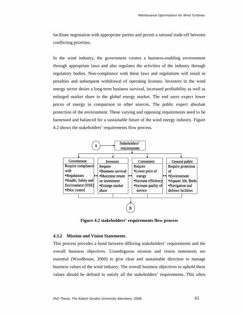
Maintenance Optimisation for Wind Turbines
PhD Thesis, The Robert Gordon University Aberdeen, 2008. 61
facilitate negotiation with appropriate parties and permit a rational trade-off between
conflicting priorities.
In the wind industry, the government creates a business-enabling environment
through appropriate laws and also regulates the activities of the industry through
regulatory bodies. Non-compliance with these laws and regulations will result in
penalties and subsequent withdrawal of operating licenses. Investors in the wind
energy sector desire a long-term business survival, increased profitability as well as
enlarged market share in the global energy market. The end users expect lower
prices of energy in comparison to other sources. The public expect absolute
protection of the environment. These varying and opposing requirements need to be
harnessed and balanced for a sustainable future of the wind energy industry. Figure
4.2 shows the stakeholders’ requirements flow process.
Figure 4.2 stakeholders’ requirements flow process
4.3.2 Mission and Vision Statements
This process provides a bond between differing stakeholders’ requirements and the
overall business objectives. Unambiguous mission and vision statements are
essential (Woodhouse, 2000) to give clear and sustainable direction to manage
business values of the wind industry. The overall business objectives to uphold these
values should be defined to satisfy all the stakeholders’ requirements. This often
AStakeholders’requirements
GovernmentRequire compliancewithRegulationsHealth, Safety and Environment (HSE)Price control
ConsumersRequireLower price of
energyIncrease efficiencyIncrease quality of
service
General publicRequire protectionofEnvironmentAquatic life, BirdsNavigation anddefence facilities
B
InvestorsRequireBusiness survivalMaximise return on investmentEnlarge market share

Maintenance Optimisation for Wind Turbines
PhD Thesis, The Robert Gordon University Aberdeen, 2008. 62
results in contradicting objectives and it is imperative therefore to minimise the
variability in the objectives by translating the objectives into concise and well
communicated functions. Thus it is crucial the overall strategies align the
departmental and individual responsibilities. An overall Key Performance
Measurement (KPM) system should be designed to reflect the requirements of the
stakeholders. Figure 4.3 shows the mission and vision statements flow process.
Figure 4.3 Mission and Vision statement flow process
4.3.3 Asset Classification
Assets are basically classified into five main groups (Eyre-Jackson and Winstone,
1999), these include physical (e.g. equipment, property, etc); human (e.g. labour,
skills, knowledge etc); intellectual (e.g. data, information, patents, copy right,
design, etc); financial (e.g. money, credit, etc) and intangible (e.g. public image,
morale, goodwill, communication etc) assets. A wind farm holds a variety of these
assets, some are primary to the core business objectives and others facilitate the
performance of the primary assets. Classifying assets in this manner will draw
C
B
Considers & exceed stakeholders
requirements?
Mission & vision statements
No
Yes
Concise,well communicated
do-able?
No
Yes
Define overall businessgoals
Establish overall KPM Return on investmentRegulatory complianceRevenue generatedShareholder value
C
B
Considers & exceed stakeholders
requirements?
Mission & vision statements
No
Yes
Concise,well communicated
do-able?
No
Yes
Define overall businessgoals
Establish overall KPM Return on investmentRegulatory complianceRevenue generatedShareholder value

Maintenance Optimisation for Wind Turbines
PhD Thesis, The Robert Gordon University Aberdeen, 2008. 63
attention to assets that are indispensable to the long-term survival of the wind
industry and also elucidate boundaries and inter-dependencies of the assets. Figure
4.4 shows the asset classification flow process.
Figure 4.4 asset categorisation flow process
4.3.4 Primary Asset
Wind turbines operate within defined wind speed limits (cut-in and cut-out). The
generated energy is then transmitted and connected to the electricity network for
distribution to consumers. Effective management of wind turbines and the associated
grid connection facilities will require the formulation of asset-based business
objectives to align the overall goals of the wind farms. The objectives will include;
effective management of Health, Safety & Environmental (HSE) factors, improving
Reliability, Availability and Maintainability (RAM), minimising the Whole Life-
Cycle Costs (WLCC), and failure elimination. Desirable and achievable targets
should be set to reflect the expected level of performance. Suitable strategies for
achieving the objectives should be determined by using appropriate AM tools and
techniques.
Reliability-Centred Maintenance (RCM) is an AM technique used mostly to select
suitable maintenance strategies for physical assets (Moubray, 1991). The approach
Asset classification
Asset indispensable to
core business goal?
YesNo
C
DE
Secondary assets Primary assets
Asset classification
Asset indispensable to
core business goal?
YesNo
C
DE
Secondary assets Primary assets

Maintenance Optimisation for Wind Turbines
PhD Thesis, The Robert Gordon University Aberdeen, 2008. 64
has been applied in several industrial sectors with considerable success. The wind
industry is yet to explore the full potentials of RCM to determine appropriate
maintenance strategies for wind turbines and the associated grid connection
facilities. RCM alone is limited in determining which maintenance strategies are the
most cost effective options available. Therefore, an ALCA technique which is
defined as “…the combined evaluation of capital costs with future performance,
operating and maintenance implications, life expectancies and eventual disposal or
replacement of an asset” (Woodhouse, 2000) should be incorporated into RCM to
assess the commercial viability of maintenance activities over the life-cycle of wind
turbines. The integration of RCM and ALCA will provide a sustainable method of
determining appropriate (technically feasible and economically viable) maintenance
strategies for wind turbines and the associated grid connection facilities to maximise
the return on investment in wind farms (Andrawus et al. 2006b & c).
Appropriate Key Performance Indicators (KPI) and the measurement systems should
be designed (Liyanage and Kumar, 2001) to align the maintenance activities and the
overall strategic business values. Actual performance should be evaluated
periodically and checked against intended targets. This will provide a baseline for
maintenance optimisation to achieve the best combination of costs, risks and
performances. Gaps and opportunities should be identified continuously and
appropriate strategies to harvest the benefits should be determined and implemented.
Figure 4.5 shows the flow process of primary assets.
4.3.5 Secondary Assets
This section discusses the secondary assets which facilitate the performance of the
primary assets discussed in subsection 4.3.4.
4.3.5.1 Data
The significance of collecting and storing the correct type of data from the
commencement of the AM process has been emphasised by Townsend (1998),
Hammond and Jones (2000), Sherwin (2005). Improving the reliability, availability
and maintainability of wind turbines and the associated grid connection facilities

Maintenance Optimisation for Wind Turbines
PhD Thesis, The Robert Gordon University Aberdeen, 2008. 65
will depend on the availability of useful historical failure and maintenance data. It is
imperative therefore to have a comprehensive inventory (including specific location)
of all wind turbines and grid connection facilities in an integrated asset register and
data management system. The system should be robust to accommodate sequential
recording of maintenance and failure data in an RCM format. This will keep the
maintenance track record of each asset in a meaningful format that can be used for
optimisation processes and for an informed decision making process.
Figure 4.5 primary asset flow process
D
Wind turbines and gridconnection facilities
Establish strategyUseRCM/FMECA to determine appropriatemaintenance strategies
Define asset business objectives
Improve reliability of turbines
Improve wind farm availability
Minimise Life Cycle Costs
Failure eliminationManage HSE
Performance according to
targets?
Optimise strategiesUse Delay-time mathematic-al modelSystem failure models-Monte Carlo simulation RCA
No
Yes
Yes
F
No
Any room forimprovement?
Performance according to
target?
Yes
NoIntegrated asset register and data management
Identify gaps, opportunities & strategies
Benchmark
Set targetsAvailability = 100%Reliability = 99%Number of injuries = 0
Set Performance Measurement for KPIAvailability= MTBF
MTBF + MTTR + PM Reliability= MTTF
MTTF + MTTR
No of injuries
Evaluate the economics Use ALCA to ensure strategies are the most cost effective options.
Establish dynamic KPIAvailability of wind turbines
Failure rates of windturbines
Maintenance efficiencyand effectivenessInjuries
Evaluate performance periodically

Maintenance Optimisation for Wind Turbines
PhD Thesis, The Robert Gordon University Aberdeen, 2008. 66
4.3.5.2 Workforce
The work force ensures effective operation and maintenance (O&M) of wind
turbines and the associated grid connection facilities to achieve the expected level of
performance. The quest for excellent performance revolves around a competent
workforce with the right people on the right jobs, having manageable work backlogs
and zero human error. Achieving this level of excellence will require an effective
training and communication scheme, clear work procedures, team work and
effective shift and reward systems. The performance of individuals should be
evaluated periodically to identify training needs for the purposes of continuous staff
development. Figure 4.6 shows the flow process of the work force.
Figure 4.6 secondary assets flow process
4.3.6 The overall continuous performance improvement
This process involves periodic evaluation of the overall business performance of
wind farms to satisfy all the requirements of the stakeholders. The overall
Performance Measurement (PM) will indicate the level of success or failure attained
in the period under consideration; this will reveal the gaps and opportunities on a
continuous basis. Furthermore, it will motivate the desire to determine and
Define business objectives Right people on right jobs Achieve competency
Workforce
Set target Human error= 0% Minimum work backlog
F
Performance according to
target?
No
Evaluate performance periodically
Identify opportunities and implement strategies
Yes
E
Establish strategies Effective training &
communication scheme Clear work procedures Team work Effective shift & reward
system
Define business objectives Right people on right jobs Achieve competency
Define business objectives Right people on right jobs Achieve competency
Workforce
Set target Human error= 0% Minimum work backlog
F
Performance according to
target?
No
Evaluate performance periodically
Identify opportunities and implement strategies
Yes
E
Establish strategies Effective training &
communication scheme Clear work procedures Team work Effective shift & reward
system
Establish strategies Effective training &
communication scheme Clear work procedures Team work Effective shift & reward
system

Maintenance Optimisation for Wind Turbines
PhD Thesis, The Robert Gordon University Aberdeen, 2008. 67
implement appropriate strategies that will bridge the identified gaps and to explore
new opportunities. Nonetheless, if no significant improvements are achieved by
applying the appropriate strategies and the root-causes cannot be identified, then
benchmarking (Benson and McGregor, 2005) against pace-setters within or across
the industry should be used to yield useful success factors that will drive the
continuous performance improvement process. Figure 4.7 shows the process flow of
the overall continuous performance improvement.
Figure 4.7 continuous performance improvement flow process
4.4 THE OVERALL PICTURE
The overall picture showing the holistic interaction and interdependencies of the
asset management processes is shown in figure 4.8. This represents the structured
model for asset management in the wind industry.
4.5 THE BENEFITS OF THE SYSTEM
The model when fully implemented will aid long-term survival of businesses
operating in the wind energy industry as well as maximising the return on
investments in wind farms.
Yes
Yes
No
Identify gap
Any opportunity/room for
improvement ?
Performanceaccording to overall
business goals?
No
Identify/implement most cost effective strategies
Evaluate overall performance periodicallyF Continuous performance
improvement
G
Performanceaccording to overall
business goals?
Benchmark No
Yes
Yes
Yes
No
Identify gap
Any opportunity/room for
improvement ?
Performanceaccording to overall
business goals?
No
Identify/implement most cost effective strategies
Evaluate overall performance periodicallyF Continuous performance
improvement
G
Performanceaccording to overall
business goals?
Benchmark No
Yes

Maintenance Optimisation for Wind Turbines
PhD Thesis, The Robert Gordon University Aberdeen, 2008. 68
Figure 4.8 the overall flow process of AM in the wind industry
Stakeholders will be kept in touch with all the necessary information they will
require to perform their task effectively.
Define business objectives
• Right people onright jobs
• Competency
Set target
• Human error= 0%• Minimum work
back log
Establish strategies
•Effective training •Clear work procedures•Effective communication
•Team work•Effective reward system
Stakeholders’requirements
Government
Require compliance with • Regulations• Health, Safety and Environment (HSE)
• Price control
ConsumersRequire
• Lower price of energy• Increase in efficiency• Increase in quality of service
General Public
Require protection of • Environment• Aquatic life, Birds etc• Navigation and defence facilities
Investors
Require
• Business survival• Profit maximisation• Enlarge market share• Minimise life cycle cost
Consider & exceed stakeholders
requirements?
Mission & vision statements
No
Yes
Concise, wellcommunicated
do-able?
No
Yes
Define overall business goals
Establish overall KPM
• Return on investment• Regulatory compliance• Revenue generated• Shareholder value added
Assets categorisation
Asset indispensable to
core business objectives?
Yes
No
D
Set performance measurement
• Availability= MTBFMTBF + MTTR + PM
• Reliability= MTTFMTTF + MTTR
• No of injuries
Evaluate the economics
Use• ALCA to ensure strategies are the most cost effective options(economically viable)
Establish dynamic KPI
• Availability of turbine• Failure rates of turbine• Maintenance efficiency
& effectiveness• Injuries
Primary Assets
Wind turbines & gridconnection facilities
Define objectives
• Improve reliability • Improve availability • Minimise LCC • Eliminate failures• Manage HSE
Establish strategyUse• RCM/FMECA to determine appropriate maintenance strategies (technically feasible)
Evaluate performance periodically
Inte
grat
ed a
sset
regi
ster
, da
ta a
nd in
form
atio
n m
an
age
men
t
B
C
Set targets
• Availability= 99%• Reliability = 99%• No of injuries= 0
Identify opportunities and implement strategy
Workforce
Evaluate performance periodically
Yes
Yes
No
Identify gap
room for any improvement ?
Performanceaccording to overall
business goals?
No
Identify/implement mostcost effective strategy
Evaluate overall performance periodically
Continuous performance improvement
G
Yes
Yes
Performance according to
targets?
Optimise strategies
Use• Mathematical models• System failure models • Root Cause Analysis
Any room forimprovement?
Benchmark
Performance according to
target?
Identify gaps, opportu-
nities & strategies
F
Performance according to target?
No
Yes
Yes
Terminate
Start
E
No
No
Performanceaccording to overall
business goals?
Benchmark
No
Yes
Maintenance Optimisation for Wind Turbines
PhD Thesis, The Robert Gordon University Aberdeen, 2008. 69
The system will preserve knowledge and improve the quality of decision making
on crucial issues such as the Health, Safety and Environment (HSE), Operational
& Maintenance etc through out the life-cycle of wind farms.
The system will improve the ability to trace causes of incidents by providing a
specific operation and maintenance diagnosis of equipment to the end user. This
will reduce the number of operational incidents such as emergency shutdowns.
Maintenance will be based on observed conditions. This will reduce the number
of down-times due to breakdowns, defects or damage, thus improving the
productivity of wind turbines and also reducing the cost of energy generation.
Replacements or overhauls of components in good operating condition will be
avoided.
The time interval between repairs and overhauls will be maximised through an
optimisation process. This will allow better planning of suitable maintenance
periods, logistics, spare holding and the associated man-hours.
Access and logistic costs will be reduced significantly.
The overall return on the investments in wind farms will be maximised.
4.6 PRACTICAL IMPLEMENTATION
This section discusses some institutional barriers in the way of practical
implementation of the AM model as well as individual responsibilities to make it
happen.
4.6.1 Institutional barriers
One key barrier to the practical implementation of the model is getting all the
stakeholders to recognise and accept the strategic importance of AM, and to be fully
and visibly committed to its implementation. Also, confidentiality among wind farm
operators can limit data and information sharing. This will affect the update of the
data base which is fundamental to long-term sustenance of the system.

Maintenance Optimisation for Wind Turbines
PhD Thesis, The Robert Gordon University Aberdeen, 2008. 70
4.6.2 Responsibilities
The right climate and a mechanism to make known the strategic importance of AM
to the wind industry are fundamental to successful implementation. It is imperative
that all the key stakeholders should take responsibilities as discussed below:
National
Government should, through appropriate policies and bye-laws, ensure that the wind
farm operators take full responsibility of maintaining assets within the wind industry
in the wider context of asset management methodology.
Company
The establishment of a policy at the national level to ensure practical
implementation of AM in the wind industry must be supported with a significant
allocation of human, material and financial resources. To this end, wind farm
management must be fully and visibly committed before the system can yield its rich
dividends. The management must be committed to initiating the required
expenditure as rapidly as possible at the start of the programme and maintaining it
while the programme continues. It is important to state that the wind farm operators
should strive to be the primary custodian of the model, even if government is
reluctant to support the system.
Workforce
The commitment of the entire personnel to the implementation of AM will be the
driving force to ensure success. The degree of benefit will be directly proportional to
the level of commitment of the personnel. It is paramount that the entire workforce
accepts the change and to be fully committed to the implementation so that the full
benefits of the system can be harvested.
4.7 SUMMARY
The wind energy industry is face with incompatible stakeholders’ requirements and
the lack of a holistic framework to harness stakeholders’ needs with assets technical
issues. A structured model for asset management in the wind industry was

Maintenance Optimisation for Wind Turbines
PhD Thesis, The Robert Gordon University Aberdeen, 2008. 71
developed. In the development of the model, AM processes, tools and techniques
existing in other industries were drawn down and integrated for the effective
management of wind farms. Crucial requirements for effective management of wind
farms have been identified and transformed into AM processes. These processes
were logically arranged to form the structure of the model. Each process was
subsequently discussed and appropriately represented in a flowchart. Finally, the
overall flow process indicating a holistic interaction of decision making and asset
interdependence has been outlined by integrating the individual process chart.
The model coherently harnesses and rationalises stakeholders’ requirements and
ensures that assets remain in a satisfactory condition over the life cycle of wind
farms. Such a model initiates the basic concept of AM in the wind industry as a
prelude to developing dedicated AM software for the industry. The activities
presented in the “primary asset flow process” (figure 4.5) will be carried out in
chapters 5-8 due to its strategic function in the overall model.

Maintenance Optimisation for Wind Turbines
PhD Thesis, The Robert Gordon University Aberdeen, 2008. 72
CHAPTER 5
SELECTION OF A SUITABLE MAINTENANCE
STRATEGY FOR WIND TURBINES
5.1 INTRODUCTION
The previous chapters had explained that the common maintenance strategies
applied to wind turbines are inadequate to meet the current maintenance demands of
the wind energy industry. Chapter 2 highlighted the need to determine an
appropriate maintenance strategy for wind turbines using asset management tools
and techniques. In chapter 3, section 3.3, a hybrid approach comprising Reliability
Centred Maintenance (RCM) and Asset Life-Cycle Analysis (ALCA) techniques
was developed to select an appropriate maintenance strategy for wind turbines.
This chapter presents and discusses the practical application of the hybrid approach
to determine a suitable maintenance strategy for wind turbines. A generic horizontal
axis wind turbine is critically assessed in section 5.2 to determine its failure
characteristics by using the Reliability-Centred Maintenance approach. A case study
is presented in section 5.3 to demonstrate the practical application of the hybrid
RCM and ALCA to determine suitable maintenance activities for critical
components and subsystems of a 600 kW wind turbine on a 26 x 600kW wind farm.
The commercial viability of CBM activities is assessed using the ALCA technique;
taking into account geographical location, intermittent operation and value of
generation. Uncertainties in the financial calculations are risk assessed using a
probabilistic technique of the Crystal Ball Monte Carlo simulation software. Non-
financial factors are identified and assessed using a Weighted Evaluation (WE)
technique and Benefit-To-Cost ratio. Finally, the summary of the chapter is
presented in section 5.4.
5.2 APPLICATION OF RCM TO A GENERIC HORIZONTAL AXI S
WIND TURBINE
The first four RCM questions, listed in chapter 3, subsection 3.3.3, identify ways in

Maintenance Optimisation for Wind Turbines
PhD Thesis, The Robert Gordon University Aberdeen, 2008. 73
which a wind turbine already in operation can fail to perform its design intentions
and the resultant effects on the components and systems of the turbine. This is
usually referred to as a Failure Mode and Effect Analysis (FMEA).
5.2.1 Functions and performance standards of a wind turbine
The primary function of a wind turbine is to convert wind kinetic energy into
electrical energy within a defined speed limit (cut-in and cut-out wind speed). This
function is solely considered to minimise complexity in the analysis. The reader is
referred to Wind Turbine Standards IEC 61400-22 for other functions and standards
of performance.
5.2.2 Functional failures
Three functional failures are defined in view of the primary function stated in
subsection 5.2.1; these include (i) Complete loss of energy conversion capability (ii)
Partial loss of energy conversion capability and (iii) Over speeding. This broad
classification permits the analysis of critical components and subsystems that are
indispensable to the normal operation of a wind turbine.
5.2.3 Failure Mode and Effect Analysis
Failure modes for the defined functional failures are presented logically in Table 5.1.
These were further scrutinised sequentially to identify possible causes up to a third
level as shown in Appendixes A1, A2 and A3. The result of this analysis can be
applied to a generic horizontal axis wind turbine.
5.3 A CASE STUDY
In this section, a case study is presented to demonstrate the practical applicability of
the approach. The last three RCM questions determine failure consequences and
suitable maintenance tasks to mitigate the penalties. Data from a 26 x 600 kW
onshore wind farm (total capacity of 15.6 MW) operating at an average capacity
factor of 33% is used to answer the last three questions. The selection of this
category of wind farm and turbine is deliberate for a number of reasons; first,
onshore wind farms have ease of access for maintenance activities; secondly, it has

Maintenance Optimisation for Wind Turbines
PhD Thesis, The Robert Gordon University Aberdeen, 2008. 74
been suggested (Verbruggen, 2003) that the failure of a low-rated-power wind
turbine such as 600 kW does not greatly affect the revenue generation of a wind
farm because wind turbines operate stand-alone and the financial margins in the
wind industry is relatively small.
Table 5.1 Functional Failure and Failure Modes for Horizontal Axis Wind Turbines Function Functional failure Failure modes WT to covert WT-1 Complete loss WT-1-1 Catastrophic blade failure wind kinetic of energy conversion WT-1-2 Catastrophic hub failure energy into capability WT-1-3 Main bearing failure electrical WT-1-4 Main shaft failure energy WT-1-5 Shaft-gearbox coupling failure within WT-1-6 Gearbox failure defined WT-1-7 Gearbox-generator coupling failure speed limit WT-1-8 Generator failure (cut-in and WT-1-9 Meteorological system failure cut-out) WT-1-10 Premature brake activation WT-1-11 Electrical system failure
WT-1-12 Tower failure WT-1-13 Foundation failure WT-2 Partial loss of WT-2-1 Crack in blade energy conversion WT-2-2 Deteriorating blade root stiffness capability WT-2-3 Blades at different pitches WT-2-4 Dirt build-up on blades WT-2-5 Ice build-up on blades WT-2-6 Damping in blades WT-2-7 Hub spins on shaft WT-2-8 Low speed shaft misalignment WT-2-9 Nacelle not yawing WT-2-10 Nacelle yaws too slowly WT-2-11 Nacelle yaws too fast WT-2-12 Large yaw angle WT-2-13 Cable twist WT-2-14 Wind speed measurement error WT-2-15 Wind direction measurement error WT-3 Over speeding WT-3-1 Controller failure WT-3-2 Hydraulic system failure WT-3-3 Pitching system failure WT-3-4 Mechanical brake failure WT-3-5 Grid connection failure

Maintenance Optimisation for Wind Turbines
PhD Thesis, The Robert Gordon University Aberdeen, 2008. 75
5.3.1 Data Collection
Current market prices of major components of a 600kW wind turbine, including
transportation cost to site, were obtained from manufacturers. Labour requirements
for replacements of these components as well as the access costs were obtained from
the collaborating wind farm operator (see table 5.2). Historical failure data pertinent
to failure modes WT-1-1, WT-1-2, WT-1-3, WT-1-4, WT-1-6 and WT-1-8 of the
600kW turbine were extracted from the SCADA (i.e. Supervisory Control and Data
Acquisition) system for a period of 6 years. The SCADA system records failures and
the date and time of occurrence; this was used in conjunction with maintenance
Work Orders (WOs) of the same period to ascertain the specific type of failure and
the components involved. Over this period, the catastrophic failure (by
“catastrophic” in this case, we mean failures beyond repair which require
replacement of the system) of a gearbox (failure mode WT-1-6) occurred twice,
while the catastrophic failure of a generator (failure mode WT-1-8) occurred on one
occasion. Activities for inspection of wind turbines drive trains were obtained from
the collaborating wind farm operator (see table 4.3) while current market prices of
vibration monitoring systems for failure modes WT-1-3, WT-1-4, WT-1-5, WT-1-6
WT-1-7 and WT-1-8 were obtained from vendors of condition monitoring system
(see table 5.4).
5.3.2 Failure Consequences
Our analysis is based on the following equations, using functions given in the
Glossary (Appendix B):
( )
++++=100
1 ATOLdLdTPITIT
VCCCCTC (5.1)
RThrdyPnLB LWNNTC ×××= (5.2)
( )
××+×=100
ATdyCRdyCRAS
VNCNCTC (5.3)
( )
××××+=
10024 f
EHPRdyhcPL
CCWTRLT (5.4)
PLASLBITC TTCTCTCF +++= (5.5)
( )Td
PW+
=1
1 (5.6)

Maintenance Optimisation for Wind Turbines
PhD Thesis, The Robert Gordon University Aberdeen, 2008. 76
Table 5.2 Data for calculating failure consequences
Materials Blade Main-bearingsMain shaft Gearbox GeneratorCost of item (£) 28,000.00 7,985.00 9,024.00 50,000.00 19,000.00 Cost of transportation (£) at 4% of material cost 1,120.00 319.40 360.96 2,000.00 760.00 Cost of Loading (£) at 0.5% of material cost 140.00 39.93 45.12 250.00 95.00Cost of off loading (£) at 0.5% of material cost 140.00 39.93 45.12 250.00 95.00Value Added Tax (%) 17.5 17.5 17.5 17.5 17.5 LabourNumber of person to replace components 3 3 3 3 3Number of days required to replace components 2 2 4 3 2Work hours per day 8 8 8 8 8Skilled labour rate per hour (£) 50.00 50.00 50.00 50.00 50.00 Access costsCost of crane hire per hour including driver (£) 100.00 100.00 100.00 100.00 100.00 Number of hours per day 24 24 24 24 24Cost of crane hire/day including Mob & Demob (£) 2,400.00 2,400.00 2,400.00 2,400.00 2,400.00 Number of days 3 3 4 4 3Value Added Tax (%) 17.5 17.5 17.5 17.5 17.5 Production lossLead time to supply material (days) 180 21 30 120 60Lead time to hire a crane (days) 4 4 4 4 4Number of repair days including travel time 3 3 4 4 3Hours per day 24 24 24 24 24Wind turbine power rating (kW) 600 600 600 600 600Capacity factor (%) 33 33 33 33 33Cost of energy per MWh (£) 50 50 50 50 50
Table 5.3 Inspection activities of 26 x 600 kW wind turbine drive trains
Number of wind turbines in wind farm (NTWF) 26
Rated power per wind turbine 600 kWCapacity factor 33 %
6-monthly service inspection of drive train
Number of turbines serviced/day/ 2 personnel (NTSD) 1 turbine
Number of full-service per year (NFS) 2
Number of full service days/year = (NTWF / NTSD) NFS 52 days
Number of personnel (NPn) 2
Work hours per day (Whr) 6 hours
Labour rate per hour (LRT) 17 pounds
Annual cost of 6-monthly inspection = 52 x Npn x Whr x LRT 10,608.00 Pounds
Annual gearbox inspection
Number of gearbox inspected/day/2 personnel (NGB) 6
Number of inspection per year (NI) 1
Number of days = (NTWF / NGB) NI 4.333 days
Number of personnel (NPn) 2
Work hours per day (Whr) 6 hours
Labour rate per hour (LRT) 50 pounds
Annual cost of gearbox inspection = 4.33 x NPn x Whr x LRT 2,600.00 pounds
Total Annual Cost of Inspection ( 10,608.00 + 2,600.00) 13,208.00 Pounds

Maintenance Optimisation for Wind Turbines
PhD Thesis, The Robert Gordon University Aberdeen, 2008. 77
Table 5.4 CBM tasks of 26 x 600 kW wind turbine drive trains
Number of wind turbines (NTWF) 26
Rated power per wind turbine 600 kWIMU 16 channel H/W & S/W D5DA3/turbine (CIMU) 7,300 pounds
Park server/ wind farm (PSF) 2,500 pounds
Maintenance spares/ wind farm (MSF) 7,300 pounds
WEBCON/turbine/annum (WEBCON) 294 pounds
Diagonostic support vibration analysis consultancy/ wind farm/annum (DSV) 1,800 pounds
Application engineering & bearing inspection/wind farm/inspection/report (AEBI) 600 pounds
Aptitude exchange licence/wind farm/annum (AELF) 696 pounds
Annual condition based servicing of drive trains
Number of turbines serviced/day/ 2 personnel (NTSD) 6 turbine
Number of full-service per year (NFS) 1
Number of full service days/year = (NTWF / NTSD) NFS 4.33 days
Number of personnel (NPn) 2
Work hours per day (Whr) 6 hours
Labour rate per hour (LRT) 17 pounds
Costs of CBM activities
Capital Cost of Condition Monitoring (CM) System = (NTWF x CIMU)+ PSF+MSF 199,600.00 pounds
Annual maintenance cost of CM = WEBCON + DSV + AEBI + AELF 3,390.00 pounds
Annual cost of condition-based servicing of drive trains = 4.33 x NPn x Whr x LRT 884.00 pounds
( )( )T
T
dd
dPWA
+−+
=1
11 (5.7)
PWATANPV ICTBM ×= (5.8)
( ) ( ) PWAACAMPWCNPV CBMcmcmCBM ++×= (5.9)
TCCR NFA ϕ= (5.10)
∑∨==
==m
jijj
niii SWSAA
1,1
.* (5.11)
i
i
niii NPV
SBTCAA ∨
===
,1
* (5.12)
Table 5.5 shows the failure consequences of critical components of a 600kW wind
turbine expressed in financial terms. These were determined by using equation 5.5
and the data in Table 5.2, taking into account cost of material (Equation 5.1), cost of
labour (Equation 5.2), cost of access (Equation 5.3) and production losses (Equation
5.4).

Maintenance Optimisation for Wind Turbines
PhD Thesis, The Robert Gordon University Aberdeen, 2008. 78
A single day outage of a 600kW wind turbine (at 33% capacity factor and ₤50/MWh
energy value) would result to a revenue loss of about ₤237/day. Moreover onshore
wind farms have the potential to operate at higher average capacity factors which
results to a greater loss of revenue. Figure 5.1 shows the effect of capacity factors
and down times on revenue generation of a 600kW wind turbine. A month down
time at 33% and 36% capacity factors will result to a revenue loss of ₤7,128 and
₤7,776 respectively, approximately 8% of the total annual revenue. Furthermore, the
effects of two or more turbines failure on revenue generation are significantly higher
(see figure 5.2). A month outage of seven 600kW wind turbines at 33% capacity
factor will result to a revenue loss of about ₤49,896. Hence, implementing a Failure
Based Maintenance strategy only, where a certain number of wind turbines are
allowed to fail before repairs are carried out will result in a significant loss of
revenue in addition to the effect on the electricity network and cost of component
replacement, given that, the lead time to supply most of the critical components
ranges between 3-4 months.
Table 5.5 Failure consequences of critical components of a 600kW wind turbine
Failure Modes Failure consequences FC (£)TCMT TCLB TCAS PLS Total
WT-1-1 Catastrophic blade failure 34,545.00 2,400.00 8,460.00 1,663.20 47,068.20 WT-1-3 Catastrophic main bearings failure 9,851.49 2,400.00 8,460.00 1,663.20 22,374.69 WT-1-4 Catastrophic main shaft failure 11,133.36 4,800.00 11,280.00 1,900.80 29,114.16 WT-1-6 Catastrophic gearbox failure 61,687.50 3,600.00 11,280.00 1,900.80 78,468.30 WT-1-8 Catastrophic generator failure 23,441.25 2,400.00 8,460.00 1,663.20 35,964.45
5.3.3 Selection of CBM tasks
The diagram in figure 5.4 was designed to select suitable on-condition tasks also
known as the Condition-Based Maintenance activities. These were selected on the
basis that an appropriate condition monitoring task is available to detect incipient
dominant failure modes (that occur gradually with warning signs and are
independent of age) so that actions can be taken to avoid the resultant consequences
(Wiggelinkhuizen E, et al 2006; Infield D, 2004; Verbruggen T 2003; Caselitz, P et
al 1997). Condition Monitoring Systems for Wind Turbines are now commercially
available, and have been installed on wind turbines in many wind farms around the

Maintenance Optimisation for Wind Turbines
PhD Thesis, The Robert Gordon University Aberdeen, 2008. 79
world, for example; the Enertrag Wind farm in Germany (see reference page), the
Cathedral Rocks wind farm in South Australia (see reference page), etc. The
collaborating wind farm operator has installed a vibrations monitoring system on the
drive train of one of the 600 kW wind turbines as a pilot project. Indeed, installation
of vibration monitoring system on the drive train of wind turbines is now becoming
a requirement for insurance purposes.
Vibration analysis was identified as the suitable condition based maintenance
technique to mitigate dominant causes of failure modes WT-1-3, WT-1-4, WT-1-5,
WT-1-6, WT-1-7, WT-1-8, WT-1-12, WT-2-7 and WT-2-8 while strain gauge
measurements were employed for dominant causes of failure modes; WT-1-1, WT-1-
2, WT-2-1, WT-2-2, WT-2-4, WT-2-5, and WT-2-6. Catastrophic failures of critical
components such as the blades, main bearings and shaft, gearbox and associated
components, the generator and associated components, towers and foundations can
be prevented through the application of appropriate CBM activities.
Figure 5.1 Effect of capacity factor and down time on revenue generation
£0
£5,000
£10,000
£15,000
£20,000
£25,000
1 2 3 4 5 6 7 14 30 60 90 Down-time (days)
Cost
cf=0.30
cf=0.31
cf=0.32
cf=0.33
cf=0.34
cf=0.35
cf=0.36

Maintenance Optimisation for Wind Turbines
PhD Thesis, The Robert Gordon University Aberdeen, 2008. 80
Figure 5.2 the effects of two or more turbines failure on revenue generation
Figure 5.3 Failure consequences of critical components of a 600kW wind
turbine
20,000.00
40,000.00
60,000.00
80,000.00
100,000.00
120,000.00
Cos
t (£)
WT-1-1Blade failure
WT-1-3Main bearing
failure
WT-1-4Main shaft
failure
WT-1-6gearbox
failure
WT-1-8generator
failure
PLS
TCAS
TCLB
TCMT
20,000.00
40,000.00
60,000.00
80,000.00
100,000.00
120,000.00
Cos
t (£)
WT-1-1Blade failure
WT-1-3Main bearing
failure
WT-1-4Main shaft
failure
WT-1-6gearbox
failure
WT-1-8generator
failure
PLS
TCAS
TCLB
TCMT
1 2 3 4 5 6 7 14 30 60 902
3 4 5
6 7
-
20,000.00
40,000.00
60,000.00
80,000.00
100,000.00
120,000.00
140,000.00
160,000.00
Co
st (
£)
Down time (days)
Turbines1 2 3 4 5 6 7 14 30 60 902
3 4 5
6 7
1 2 3 4 5 6 7 14 30 60 902
3 4 5
6 7
-
20,000.00
40,000.00
60,000.00
80,000.00
100,000.00
120,000.00
140,000.00
160,000.00
Co
st (
£)
Down time (days)
Turbines

Maintenance Optimisation for Wind Turbines
PhD Thesis, The Robert Gordon University Aberdeen, 2008. 81
Figure 5.4 Maintenance Selection Model
5.3.4 Economic Analysis of CBM and comparison with TBM
The economic life of a wind turbine is 20 years (Lenzen and Munksgaard, 2002),
(Kaldellis and Gavras, 2000) but an analysis period of 18 years is used in this paper
to account for the 2 years all-in-service contract and obsolescence with changing
technology. The corporate organisation of the collaborating wind farm operator
utilises a discount rate of 8.2% for all financial analysis. Also, a spare pool of 1
gearbox, 1 generator, 3 blades etc is held by the wind farm under the TBM strategy.
If any of these systems fail and it can not be repaired in-situ, the failed system is
replaced with a spare before repairs are carried out and then transferred into the
spare pool (note; the maximum number of spares that can possibly be in the re-
supply chain of the wind farm at one time is beyond the scope of this paper). Using
this information and the data in tables 5.3 and 5.4, the economics of TBM and CBM
are evaluated and compared.
The Present worth (PW) and Present Worth per Annum (PWA), which is used for
discounting initial non-recurring costs and annual recurring costs respectively, are
determined by using equations 5.6 and 5.7 to obtain the values of 0.24 and 9.24
Designing out cause of failure economical?
Consequences of failure acceptable?
Designing out cause of failure practical?
Failure Based Maintenance (FBM)
YesNo
Condition monitoringeconomical?
Condition Based Maintenance (CBM)
No
Yes
Yes
No
No Life reasonably predictable?
Time Based Maintenance (TBM)
Yes
Yes
Condition monitoringpossible?
Modify plant
Yes
No
No
Designing out cause of failure economical?
Consequences of failure acceptable?
Designing out cause of failure practical?
Failure Based Maintenance (FBM)
YesNo Consequences of failure acceptable?
Designing out cause of failure practical?
Failure Based Maintenance (FBM)
YesNo
Condition monitoringeconomical?
Condition Based Maintenance (CBM)
No
Yes
Yes
No
Condition monitoringeconomical?
Condition Based Maintenance (CBM)
No
Yes
Yes
No
No Life reasonably predictable?
Time Based Maintenance (TBM)
Yes
Yes
Condition monitoringpossible?
Modify plant
Yes
No
No

Maintenance Optimisation for Wind Turbines
PhD Thesis, The Robert Gordon University Aberdeen, 2008. 82
respectively. Then, the Net Present Value (NPV) of TBM and CBM, are calculated
by using equations 5.8 and 5.9 respectively to obtain the values of £122,085 and
£239,105 respectively. The results show that scheduled inspection of the drive trains
of wind turbines is the most cost effective option over the 18 year life-cycle with a
total savings of about £117,020. Indeed, the NPV of inspection (£122,085) is less
than the initial capital cost of installing condition monitoring systems (£199,600).
5.3.5 Uncertainties and Risks Assessment
The NPV analysis deals with future costs which invariably contain uncertainties and
risks that require critical assessments to ensure the accuracy of results for valid
decision making. A probabilistic approach of ‘Crystal Ball Monte Carlo’ simulation
was used to assess the risks and uncertainties of the key variables in the Net Present
Value calculations. After a 10,000 trials, the result of the TBM simulation is
presented in table 5.6. The mean Net Present Value of the TBM is £122,407. This is
slightly greater than the calculated NPV of the TBM (subsection 5.3.4) with about
£322. The standard deviation is about £12,487 and the mean standard error is £125.
The skewness and coefficient of variability are 0.21 and 0.10 respectively.
Table 5.6 TBM Simulation Result
Statistics Forecast valuesTrials 10,000Mean 122,407.55 Median 121,936.82 Mode ---Standard Deviation 12,487.39 Variance 155,934,950.27 Skewness 0.21Kurtosis 3.04Coeff. of Variability 0.10Minimum 80,113.10 Maximum 172,893.77 Range Width 92,780.67 Mean Std. Error 124.87
The result of the CBM simulation after a 10,000 trials is presented in table 5.7. The
mean Net Present Value of the CBM is £239,070. In this case, the mean Net Present
Value of the CBM is less than its calculated NPV with about £35. The standard

Maintenance Optimisation for Wind Turbines
PhD Thesis, The Robert Gordon University Aberdeen, 2008. 83
deviation is about £19,202 and the mean standard error is about £192. The skewness
and coefficient of variability are almost zero.
Table 5.7 CBM Simulation Result
Statistics Forecast valuesTrials 10,000Mean 239,070.30 Median 238,856.63 Mode ---Standard Deviation 19,201.98 Variance 368,715,966.09 Skewness 0.04Kurtosis 3.02Coeff. of Variability 0.08Minimum 162,846.43 Maximum 309,711.35 Range Width 146,864.92 Mean Std. Error 192.02
Figures 5.5 and 5.6 show the overlay and trend chart of the NPVs of the TBM and
the CBM. The overlay chart shows no significant effect of uncertainties on the
NPVs as the two forecast are widely apart. Similarly, the trend chart clearly shows a
constant increasing NPV from TBM to CBM as shown in the figure 5.6. The trend
chart data at various percentiles are shown in table 5.8. Note the median NPV of the
TBM and CBM are £121,937 and £238,857 respectively.
Overlay Chart 1
0
200
400
600
800
1000
1200
1400
89,496.78 130,575.38 171,653.98 212,732.58 253,811.17
Fre
que
ncy Net Present Value (NPV) of
inspection
NPV of Condition BasedMaintenance
Figure 5.5 NPV overlay chart

Maintenance Optimisation for Wind Turbines
PhD Thesis, The Robert Gordon University Aberdeen, 2008. 84
Trend Chart 1
94,242.83114,242.83134,242.83154,242.83174,242.83194,242.83214,242.83234,242.83254,242.83274,242.83
Net P
resentV
alue (NP
V)
of inspection
NP
V of
ConditionB
asedM
aintenance
90.00%
50.00%
25.00%
10.00%
Median
Figure 5.6 NPV trend chart
Table 5.8 The trend Chart data at various percentages
Trend Chart Data NPV of TBM NPV of CBM90.0% 102,658.44 207,669.4650.0% 113,685.65 226,151.8625.0% 118,031.91 232,918.8210.0% 120,402.80 236,493.54Median 121,936.82 238,856.6310.0% 123,556.95 241,231.8625.0% 126,164.56 244,886.7850.0% 130,498.37 251,734.7990.0% 143,609.60 270,970.68
The sensitivity report of the TBM and CBM Net Present Value calculation are
presented in figures 5.7 and 5.8 respectively. Labour cost per hour is found to be the
most sensitive variable in the TBM Net Present Value calculation with about 64.3%
sensitivity. On the other hand, the discount rate is found to be the most insensitive
variable with about minus 31.7% sensitivity.

Maintenance Optimisation for Wind Turbines
PhD Thesis, The Robert Gordon University Aberdeen, 2008. 85
Sensitivity: Net Present Value (NPV) of inspection
-100.0% -50.0% 0.0% 50.0% 100.0%
Labour cost per hour
Park server/park
Discount rate (M28)
Diagonostic support VAconsultancy/park/annum
Figure 5.7 TBM sensitivity report
The initial cost of the condition monitoring systems (i.e. IMU 16 channel H/W &
S/W D5DA3/ turbine) is found to be the most sensitive variable in the CBM Net
Present Value calculation with about 93.3% sensitivity as shown in the figure 5.8.
Diagnostic support vibration analysis consultancy has sensitivity of about 1.1%.
Also the discount rate is found to be insensitive variable with sensitivity value of
about minus 1.1%.
Sensitivity: NPV of Condition Based Maintenance
-100.0% -50.0% 0.0% 50.0% 100.0%
IMU 16 channel H/W & S/WD5DA3/turbine
Maintenance spares/park
Aptitude exchangelicence/park/annum
Labour cost per hour
Figure 5.8 CBM sensitivity report

Maintenance Optimisation for Wind Turbines
PhD Thesis, The Robert Gordon University Aberdeen, 2008. 86
5.3.6 Evaluation of Non-financial Factors
An economic analysis based on purely financial criteria is not in itself adequate for
valid decision making (Kirk and Dell’lsola, 1995). Non-financial factors, which are
not reducible to monetary values should be identified and incorporated into the
overall economic analysis (Kishk, 2002). A maintenance strategy that is appropriate
for a specific physical asset should be reliable to uphold the integrity of the asset and
also to fulfil all statutory and health and safety requirements. These non-financial
factors are fundamental and can not be compromised in the selection of a suitable
maintenance strategy. In figure 5.9, a screening model (Kishk and Pollock, 2004) for
maintenance strategies is presented and a weight of 3 (i.e. good) was established as
the minimum standard requirement for each of the decisive criteria.
Figure 5.9 Model for screening options and criteria
Identify alternatives Establish screening criteria
Minimum requirement
satisfied?
Reliability Criteria
Health and safety Criteria
Statutory Criteria
Establish standard requirements
Collate performance data
Discard Alternative No Compile otherassessment criteria
Yes
Non-financial criteria
Collate financialdata
Life-cycle Analysis
Net Present Value
Evaluate applicability
Weighted EvaluationCollate non-financialdata
BTC ratios
Overall ranking
A
Criteria reduced
to monetaryscale?
Financial criteria
Terminate
Yes
No

Maintenance Optimisation for Wind Turbines
PhD Thesis, The Robert Gordon University Aberdeen, 2008. 87
In addition to the crucial factors, five other criteria were identified. These includes
‘ fault detection’ which is the ability to discover faults at an early stage so that
appropriate actions can be taken to avoid the consequences; ‘fault identification’
which is the ability to identify the subsystem or component most relevant to
diagnosing the fault within the shortest time possible; ‘fault diagnosis’ is the ability
to determine the cause of the fault within the shortest time possible; ‘process
recovery’ is the ease of rectifying the fault in good time and ‘Efficiency’ is the
effectiveness of restoring the asset to a normal operating condition. These were
assessed using the Weighted Evaluation (WE) technique (Kirk and Dell’lsola, 1995);
(Kishk, 2002) and the result is presented in figure 5.10. It is worth noting however,
that the non-financial factors can be subjective and figure 5.10 was established
through discussion with wind farm operators.
The WE approach consists of two processes; first, assessment criteria are identified
and the weights of their relative importance are established. These are sequentially
compared in pairs and the most vital criterion is scored according to its comparative
preference of scale 1 to 4, for example in figure 5.10, criterion ‘A’ (fault detection)
is compared with criterion ‘E’ (health and safety), E is found to be more important
than A and it is a major preference, hence the value ‘E-4’ was recorded.
The scores of each criterion are summed up (Raw Score in figure 5.10) and the final
weights jW are determined such that the maximum weight is assigned a value of 10
(Weight of importance in figure 5.10). Secondly, the rating ijS of each strategy
(TBM and CBM) in terms of each criterion is determined on a scale of 1 to 5 (i.e.
poor to excellent), for instance, the performance of CBM in terms of criterion ‘A’
(fault detection) was found to be ‘good’ (i.e. 3). These values were then multiplied
by the corresponding criterion final weights jW and the summation gives the total
score of the strategy (equation 5.11). As a rule, the best alternative A* should have
the highest total score (Kishk, 2002). In figure 5.10, the total scores of TBM and
CBM are 105 and 142 respectively; this suggests that the CBM strategy is the best
alternative.

Maintenance Optimisation for Wind Turbines
PhD Thesis, The Robert Gordon University Aberdeen, 2008. 88
Figure 5.10 Weighted Evaluation of non-financial factors of TBM and CBM
5.3.7 Benefit-To-Cost Ratio Evaluation
The benefit-to-cost (BTC) ratio evaluation combines the results of the financial and
the non-financial calculations to determine and compare the benefits derived from
the competing options. The higher the ratio the better the benefit derived from the
alternative. Equation 5.12 was used to determine the BTC ratio of TBM and CBM to
obtain the values of 0.000860 and 0.000594 respectively (figure 5.10). This indicates
that the BTC ratio of CBM strategy is very low in comparison to TBM because of
the high initial capital investments required for installing condition monitoring
systems. However, the life-cycle analysis is not complete unless the effect of failure
rate of the critical components is assessed and incorporated into the overall analysis
(Andrawus et al. 2006c).
Criteria
A. Fault detection
B. Fault identification
C. Fault diagnosis
D. Process recovery
E. Health & safety
F. Reliability
G. Efficiency
Criteria Importance4-Major preference3-Medium preference2-Minor preference1-(letter/letter)-no preference
Each scores one point
Raw Score
Weight of importance
AN
ALY
SIS
MA
TR
IX
2. Condition BasedMaintenance
A/BA -4
D/FF -4
F -4F -4
D -3C -3
B -3A -4
D -4
E-4
E/FE -4
F -4
D -4B -4
E-4E -4
D -4E -4
AG F E D C B
90 20 21 17 3 8
41* 10 10 8 2 4
33 4 3 1 2 2123 40 30 8 4 8
Total
105
142
NPV
£122,085.03
£239,105.71
CR
ITE
RIA
SC
OR
ING
MA
TR
IXA
ltern
ativ
es 0.000860
0.000594
BTC Ratio
Excellent - 5; Very good -4; Good -3; Fair -2; Poor -1
33 3 5 4 3 3123 30 50 32 6 12
1. Time Based Maintenance
Criteria
A. Fault detection
B. Fault identification
C. Fault diagnosis
D. Process recovery
E. Health & safety
F. Reliability
G. Efficiency
Criteria Importance4-Major preference3-Medium preference2-Minor preference1-(letter/letter)-no preference
Each scores one point
Raw Score
Weight of importance
AN
ALY
SIS
MA
TR
IX
2. Condition BasedMaintenance
A/BA -4
D/FF -4
F -4F -4
D -3C -3
B -3A -4
D -4
E-4
E/FE -4
F -4
D -4B -4
E-4E -4
D -4E -4
A/BA -4
D/FF -4
F -4F -4
D -3C -3
B -3A -4
D -4
E-4
E/FE -4
F -4
D -4B -4
E-4E -4
D -4E -4
AG F E D C B
90 20 21 17 3 8
AG F E D C B AG F E D C B
90 20 21 17 3 8 90 20 21 17 3 8
41* 10 10 8 2 4 41* 10 10 8 2 4
33 4 3 1 2 2 33 4 3 1 2 2123 40 30 8 4 8 123 40 30 8 4 8
Total
105
Total
105
142
NPV
£122,085.03
£239,105.71
CR
ITE
RIA
SC
OR
ING
MA
TR
IXA
ltern
ativ
es 0.000860
0.000594
BTC Ratio
Excellent - 5; Very good -4; Good -3; Fair -2; Poor -1
33 3 5 4 3 3 33 3 5 4 3 3123 30 50 32 6 12 123 30 50 32 6 12
1. Time Based Maintenance
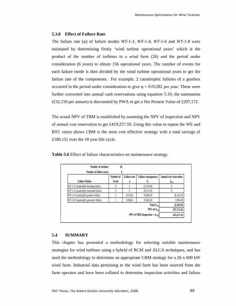
Maintenance Optimisation for Wind Turbines
PhD Thesis, The Robert Gordon University Aberdeen, 2008. 89
5.3.8 Effect of Failure Rate
The failure rate (φ) of failure modes WT-1-3, WT-1-4, WT-1-6 and WT-1-8 were
estimated by determining firstly ‘wind turbine operational years’ which is the
product of the number of turbines in a wind farm (26) and the period under
consideration (6 years) to obtain 156 operational years. The number of events for
each failure mode is then divided by the wind turbine operational years to get the
failure rate of the components. For example, 2 catastrophic failures of a gearbox
occurred in the period under consideration to give φ = 0.01282 per year. These were
further converted into annual cash reservations using equation 5.10; the summation
(£32,150 per annum) is discounted by PWA to get a Net Present Value of £297,172.
The actual NPV of TBM is established by summing the NPV of inspection and NPV
of annual cost reservation to get £419,257.59. Using this value to repeat the WE and
BTC ratios shows CBM is the most cost effective strategy with a total savings of
£180,151 over the 18 year life cycle.
Table 5.6 Effect of failure characteristics on maintenance strategy.
Number of turbines 26
Number of failure years 6
Number of Failure rate Failure consequences Annual cost reservation Failure Modes Event α FC ACR
WT-1-3 Catastrophic bearings failure 0 0 22,374.69 0WT-1-4 Catastrophic mainshaft failure 0 0 29,114.16 0WT-1-6 Catastrophic gearbox failure 2 0.01282 78,468.30 26,156.10
WT-1-8 Catastrophic generator failure 1 0.00641 35,964.45 5,994.08
Total ACR 32,150.18 NPV of ACR 297,172.56
NPV of TBM (Inspection + ACR) 419,257.59
5.4 SUMMARY
This chapter has presented a methodology for selecting suitable maintenance
strategies for wind turbines using a hybrid of RCM and ALCA techniques, and has
used the methodology to determine an appropriate CBM strategy for a 26 x 600 kW
wind farm. Industrial data pertaining to the wind farm has been sourced from the
farm operator and have been collated to determine inspection activities and failure

Maintenance Optimisation for Wind Turbines
PhD Thesis, The Robert Gordon University Aberdeen, 2008. 90
history of the wind turbines. Current market prices of critical components of the
wind turbines as well as the condition monitoring systems have been sourced from
manufactures and vendors. The RCM approach has been used to determine wind
turbines failure modes, causes and effects. Failure consequences of critical
components have been determined and expressed in financial terms.
Suitable CBM tasks have been determined and compared with TBM activities using
the ALCA technique. In the comparison, the NPV of TBM and CBM has been
calculated. It has been shown that comparison of the NPV of the two strategies is not
absolute for a valid decision making since the NPV considers only financial criteria.
The non-financial aspects of the two strategies have been identified and assessed
using the ‘WE technique’ and ‘benefit-to-cost ratio’. Failure data was extracted from
the SCADA system of the wind farm, and was validated by the maintenance work
orders of the same period. The failure rate of the critical components was calculated
and included in the analysis since the selection of a suitable maintenance strategy
depends upon the failure characteristics of the wind turbines. The overall result
shows CBM is the most cost effective option with a total savings of about £180,152
over 18 year life-cycle.

Maintenance Optimisation for Wind Turbines
PhD Thesis, The Robert Gordon University Aberdeen, 2008. 91
CHAPTER 6
ASSESSMENT OF WIND TURBINES
FIELD FAILURE DATA
6.1 INTRODUCTION
This chapter and the next, will demonstrate the practical application of one the
quantitative maintenance optimisation approach known as the Modelling System
Failures (MSF). This chapter focuses on the analyses of field failure and
maintenance data of horizontal axis wind turbines collected from wind farms. The
characteristics of the collected data are discussed in section 6.2. The data are
analysed in section 6.3 using Maximum Likelihood Estimation (MLE) to estimate
the shape (β) and scale (η) parameters of the Weibull distribution for critical
components and subsystems of a particular type of 600 kW wind turbine. Weibull
probability plots, reliability graphs, failure verses time plots, and probability density
function graphs for the components and subsystems are presented along side the
estimated shape (β) and scale (η) parameters. A case study of the 26 x 600 kW wind
farm is presented in section 6.4 to demonstrate the practical application of the
estimated β and η values to determine and optimise maintenance activities for the
critical components and subsystems of the wind turbine. The summary of the chapter
is presented in section 6.5.
6.2 DATA COLLECTION
In addition to the failure data collected from the 26 x 600 kW wind farm, more data
were sourced from 26 wind farms (comprising turbines of different capacity ratings)
located within the same geographical region. The collected data was first organised
in accordance with the type, design and capacity of the wind turbines. This was
further re-grouped according to subsystems and components of the wind turbine and
then re-arranged in order of failure modes and dates. Tables 6.1, 6.2, 6.3 and 6.4
contain the field failure data for the main shaft, main bearings, gearbox and the
generator respectively of 600 kW wind turbines.

Maintenance Optimisation for Wind Turbines
PhD Thesis, The Robert Gordon University Aberdeen, 2008. 92
In order to evaluate the wind farms in confidentiality, they were labelled
alphabetically (A to Z; AB); WF-C in column 1 of Table 6.1 denotes Wind Farm C.
The wind turbines were named according to their respective wind farms; WF-A-WT-
10 (Table 6.2, column 2) denotes Wind Farm A-Wind Turbine number 10. The
manufacturers of the failed components were numbered and recorded in column 3 of
tables 6.1-6.4. The fail-date and fail-time from the base-date as well as the causes of
failure are recorded in the same tables. Note that table 6.4 shows additional
information about the serial numbers of the failed generators. This information is
essential to identify re-occurring failure modes and to effectively trace the failure
history of each component or subsystem of the wind turbine.
Table 6.1 Failure Data for the Main Shafts of 600 kW Wind Turbine
Wind Farm (WF )
Wind Turbine (WT )
Component Manufacturer
Fail date dd/mm/yyyy Fail time (days) Main shaft
Causes of failure
WF-C WF-C-WT-13 2 "19/11/2003" 315 F Other
WF-K WF-K-WT-7 5 "01/03/2004" 424 F Poor design
WF-F WF-F-WT-16 1 "07/05/2004" 492 F Unknown
WF-A WF-A-WT-27 1 "13/06/2004" 529 F Fatigue
WF-L WF-L-WT-3 7 "29/12/2004" 698 F Fatigue
WF-N WF-N-WT-3 2 "25/07/2005" 936 F Fatigue
WF-M WF-M-WT-3 7 "14/06/2006" 1233 F Fatigue
Table 6.2 Failure Data for the Main Bearings of 600 kW Wind Turbine
Wind Farm (WF )
Wind Turbine (WT)
Component Manufacturer
Fail date dd/mm/yyyy
Fail time (days) Main Bearings
Causes of failure
WF-A WF-A-WT-10 1 "29/01/2003" 29 F Poor design
WF-B WF-B-WT-4 2 "09/05/2003" 129 F Poor design
WF-A WF-A-WT-13 1 "19/05/2003" 139 F Poor design
WF-A WF-A-WT-3 1 "27/06/2003" 178 F Poor design
WF-C WF-C-WT-4 2 "31/07/2003" 212 F Unknown
WF-D WF-D-WT-13 1 "05/11/2003" 309 F Unknown
WF-A WF-A-WT-34 4 "10/02/2004" 406 F Fatigue
WF-E WF-E-WT-2 3 "15/05/2004" 500 F Poor design
WF-A WF-A-WT-22 1 "15/12/2004" 714 F Fatigue
WF-D WF-D-WT-13 1 "27/12/2004" 726 F Fatigue
WF-A WF-A-WT-26 1 "17/01/2005" 747 F Fatigue
WF-A WF-A-WT-34 3 "18/01/2005" 748 F Fatigue

Maintenance Optimisation for Wind Turbines
PhD Thesis, The Robert Gordon University Aberdeen, 2008. 93
Table 6.3 Failure Data for the Gearboxes of 600 kW Wind Turbine
Wind Farm (WF )
Wind Turbine (WT)
Component Manufacturer
Fail date dd/mm/yyyy
Fail time (days)
HSS bearing
IMS bearing
Gear wheels
Key way
Gearbox catastrophic
Causes of failure
WT-F WF-F-WT-1 8 "24/11/1999" 329 F S S S F "Unknown"
WT-F WF-F-WT-18 8 "13/01/2000" 378 F S F F F "Fatigue"WT-F WF-F-WT-24 8 "26/03/2001" 815 F S S F F "Fatigue"WT-F WF-F-WT-07 8 "23/07/2001" 934 F S S F S "Fatigue"WT-F WF-F-WT-15 8 "19/11/2001" 1043 F S F S S "Fatigue"
WF-A WF-A-WT-8 9 "05/05/2003" 1585 F F S S S "Fatigue"WF-A WF-A-WT-14 9 "06/06/2003" 1649 F F S S S "Fatigue"WF-A WF-A-WT-23 9 "04/08/2003" 1676 F S S S S "Fatigue"WF-A WF-A-WT-9 9 "27/08/2003" 1699 F F S S S "Fatigue"WF-B WF-B-WT-6 9 "11/09/2003" 1714 F F S S S "Fatigue"
WF-B WF-B-WT-10 9 "04/11/2003" 1768 S S S S S "Fatigue"
WF-B WF-B-WT-6 10 "04/11/2003" 1768 S S S S S "Fatigue"WF-B WF-B-WT-14 9 "22/11/2003" 1786 S S S S S "Fatigue"WF-F WF-F-WT-19 9 "18/06/2004" 1985 S S F S S "Fatigue"
WF-G WF-G-WT-9 9 "30/06/2004" 2006 F F S S F "Unknown"WF-A WF-A-WT-33 8 "09/10/2004" 2107 S S F S F "Fatigue"WF-A WF-A-WT-1 8 "18/10/2004" 2116 S S S S S "Fatigue"
WF-A WF-A-WT-19 8 "30/10/2004" 2128 S S S S S "Fatigue"WF-C WF-C-WT-7 11 "01/11/2004" 2130 F S F S S "Fatigue"WF-D WF-D-WT-20 10 "04/02/2005" 2225 S S F S S "Poor design"WF-A WF-A-WT-19 10 "02/04/2005" 2282 S S F S S "Poor design"WF-D WF-D-WT-2 8 "11/05/2005" 2321 S S S S S "Poor design"
To illustrate the importance of the additional information in the table 6.4, consider
the failure data recorded in row 3 of the table. A generator with a serial number
GSN-2 failed in wind turbine 22 of wind farm F. Also in row 4 of the table, another
generator failure is recorded with a serial number GSN-2 but this time in wind
turbine 15 of the same wind farm. It will be noticed that the serial numbers of the
generators are the same, indeed, it is the same generator. The first failure of the
generator in wind turbine 22 was due to bearing failure, it was removed for repairs
and the turbine was fitted with a spare. The failed generator (GSN-2) was repaired
and transferred into the spare pool.
The generator in wind turbine 15 failed and it was fitted with the GSN-2 from the
spare pool. The generator (GSN-2) eventually failed catastrophically as a result of a
stator winding failure. A similar failure event is recorded in rows 9-11 of the table. It

Maintenance Optimisation for Wind Turbines
PhD Thesis, The Robert Gordon University Aberdeen, 2008. 94
is worth noting that this type of detailed recording of failure data was found only in
wind farm F and is specific to the generators.
Table 6.4 Failure Data for the Generators of 600 kW Wind Turbine Wind Farm (WF )
Wind Turbine (WT)
Serial number
Component Manufacturer
Fail date dd/mm/yyyy
Fail time (days)
Windings Bearings
Generator catastrophic
Causes of failure
WF-F WF-F-WT-1 GSN-1 4 "24/02/1997" 55 S S F FatigueWF-F WF-F-WT-22 GSN-2 4 "15/02/1998" 411 S F S FatigueWF-F WF-F-WT-15 GSN-2 4 "01/06/2000" 424 F S F FatigueWF-F WF-F-WT-15 GSN-3 4 "01/03/1999" 789 S F S FatigueWF-F WF-F-WT-18 GSN-4 4 "01/06/1999" 881 S F S OtherWF-F WF-F-WT-12 GSN-5 4 "01/12/2000" 548 S S F OtherWF-F WF-F-WT-12 GSN-6 4 "01/10/1999" 1003 F S S Poor DesignWF-F WF-F-WT-17 GSN-7 4 "15/12/1999" 1080 F S S UnknownWF-F WF-F-WT-15 GSN-7 4 "01/01/2002" 746 F S S Poor DesignWF-F WF-F-WT-15 GSN-7 4 "01/07/2002" 181 F S S Poor DesignWF-F WF-F-WT-5 GSN-8 4 "08/01/2000" 1307 S F S FatigueWF-F WF-F-WT-24 GSN-9 4 "08/01/2000" 1307 S S F Poor DesignWF-F WF-F-WT-16 GSN-10 4 "01/11/2000" 1399 S F S Poor DesignWF-F WF-F-WT-7 GSN-11 4 "01/06/2002" 1977 S F S Poor DesignWF-D WF-D-WT-26 GSN-12 4 "21/01/2003" 2211 S F S FatigueWF-A WF-A-WT-29 GSN-13 4 "29/01/2003" 2219 S F S FatigueWF-A WF-A-WT-20 GSN-14 4 "09/04/2003" 2289 S F S FatigueWF-C WF-C-WT-11 GSN-15 4 "09/05/2003" 2319 S F S FatigueWF-A WF-A-WT-18 GSN-16 4 "09/06/2003" 2349 F S S FatigueWF-A WF-A-WT-8 GSN-17 4 "24/06/2003" 2364 S F S FatigueWF-D WF-D-WT-4 GSN-18 4 "07/08/2003" 2409 S F S FatigueWF-D WF-D-WT-2 GSN-19 4 "28/08/2003" 2430 F S S FatigueWF-D WF-D-WT-27 GSN-20 4 "15/09/2003" 2445 S F S FatigueWF-A WF-A-WT-21 GSN-21 4 "11/11/2003" 2535 F F F FatigueWF-H WF-H-WT-11 GSN-22 4 "13/11/2003" 2537 S F S FatigueWF-A WF-A-WT-7 GSN-23 4 "29/12/2003" 2553 S F S FatigueWF-A WF-A-WT-20 GSN-24 4 "29/01/2004" 2584 S F S OtherWF-C WF-C-WT-8 GSN-25 4 "04/03/2004" 2618 S F S OtherWF-E WF-E-WT-20 GSN-26 4 "25/03/2004" 2639 F S S Poor DesignWF-F WF-F-WT-20 GSN-27 4 "25/03/2004" 2639 S S S UnknownWF-I WF-I-WT-1 GSN-28 4 "20/04/2004" 2665 S F S Poor DesignWF-D WF-D-WT-15 GSN-29 4 "23/04/2004" 2668 S S S FatigueWF-A WF-A-WT-1 GSN-30 4 "04/05/2004" 2679 F F F Poor DesignWF-D WF-D-WT-27 GSN-31 4 "07/05/2004" 2682 S F S Poor DesignWF-E WF-E-WT-4 GSN-32 4 "18/06/2004" 2724 S F S Poor DesignWF-I WF-I-WT-6 GSN-33 4 "26/06/2004" 2732 S F S Poor DesignWF-G WF-G-WT-9 GSN-34 4 "08/07/2004" 2744 S S S OtherWF-A WF-A-WT-29 GSN-35 4 "13/07/2004" 2749 S F S Poor DesignWF-A WF-A-WT-17 GSN-36 4 "16/07/2004" 2752 S F F Poor DesignWF-C WF-C-WT-19 GSN-37 4 "30/07/2004" 2766 S S S Poor DesignWF-C WF-C-WT-10 GSN-38 4 "12/08/2004" 2779 S S F Poor DesignWF-E WF-E-WT-11 GSN-39 4 "17/09/2004" 2815 S F S Poor DesignWF-D WF-D-WT-28 GSN-40 4 "21/09/2004" 2819 S F S Poor DesignWF-E WF-E-WT-16 GSN-41 4 "25/10/2004" 2853 F S S FatigueWF-E WF-E-WT-13 GSN-42 4 "07/11/2004" 2866 F S S FatigueWF-I WF-I-WT-7 GSN-43 4 "29/12/2004" 2918 F S S Poor DesignWF-A WF-A-WT-24 GSN-44 4 "02/01/2005" 2922 F S S Poor DesignWF-A WF-A-WT-6 GSN-45 4 "28/02/2005" 2969 F F F Poor DesignWF-I WF-I-WT-13 GSN-46 4 "07/04/2005" 3007 S F S Poor DesignWF-A WF-A-WT-19 GSN-47 4 "26/04/2005" 3026 S F S Poor DesignWF-J WF-J-WT-9 GSN-48 4 "12/09/2005" 3165 S F S Poor Design

Maintenance Optimisation for Wind Turbines
PhD Thesis, The Robert Gordon University Aberdeen, 2008. 95
6.3 SHAPE AND SCALE PARAMETERS OF COMPONENTS AND
SUBSYSTEMS OF 600 kW WIND TURBINE
The shape and scale parameters for components and subsystems of the various types
of wind turbines are estimated in this section. It was mentioned previously that the
value of β describes the failure pattern of the equipment, that is, β <1 means a
reducing failure pattern, β =1 signifies a constant failure pattern and β >1 indicates
an increasing failure pattern. The scale parameter (η) denotes the characteristic life
of the equipment; the time at which there is probability of approximately 0.632 that
the equipment will have failed.
The reducing failure pattern (β <1) usually known as the infant mortality denotes
failures that occur at the early-life of equipment and the likelihood of occurrence
reduces as the age of the equipment increases. The constant failure pattern (β =1)
represents failures that are independent of equipment age, that is, the likelihood of
occurrence is invariable through out the life-cycle of the equipment. Lastly, the
increasing failure pattern (β >1) commonly referred to as wear-out symbolises
failures that occur at the later life of equipment, that is, the likelihood of occurrence
increases with the age of the equipment.
The shape (β) and scale (η) parameters of critical components and subsystems of the
600 kW wind turbine are estimated using the ReliaSoft Weibull ++7 software. The
results are presented in table 6.5. The probability distribution and the parameter
estimation technique are shown in columns 3 and 4 of the table respectively. In the
analysis, the Fisher Matrix (FM) confidence bound method and median (MED)
ranking was used to underpin the statistical evaluation. The Mean Life or Mean Time
Between Failures (MTBF) of each of the critical components and subsystems are
presented in column 10 of the same table. Note that the scale parameters and the
mean time between failures are in days.

Maintenance Optimisation for Wind Turbines
PhD Thesis, The Robert Gordon University Aberdeen, 2008. 96
Table 6.5 Shape and Scale parameters for critical components of 600 kW wind
turbine
Sub-system Components Distribution Analysis Shape
(β)Scale (η)
Likeli- hood Failed Suspended
Mean Life (MTBF)
BladeMain shaft Weibull-2P MLE 1.43 6389 -72.90 7 70 5807
Main bearing Weibull-2P MLE 1.09 3835 -112.79 12 65 3711
Gearbox Weibull-2P MLE 1.05 29051 -56.99 5 72 28521
Gears Weibull-2P MLE 2.50 5715 -75.10 7 70 5070
HSS bearings Weibull-2P MLE 1.52 7244 -125.00 12 64 6528
IMS bearings Weibull-2P MLE 3.63 4694 -53.99 5 72 4232
Key way Weibull-2P MLE 0.84 101790 -35.69 3 74 111720
Generator Weibull-2P MLE 1.11 17541 -98.70 9 68 16888
Bearings Weibull-2P MLE 1.39 4956 -300.00 31 46 4524
Windings Weibull-2P MLE 1.62 7158 -155.00 15 62 6412
6.3.1 The Main Shaft
The estimated values of β and η for the main shaft are 1.43 and 6389 respectively.
The β value of 1.43 indicate a wear out failure pattern while the η value of 6389
implies that there is a probability of approximately 0.632 that all the main shafts in a
wind farm of 600 kW turbine would have failed within 6389 days or approximately
18 years, given the assessed failure behaviour of the main shafts and the current
maintenance strategy employed. The Weibull plot (graphical data analysis) for the
main shafts failure data is shown in figure 6.1.
Figure 6.1 Main Shaft Weibull Plot
β=1.4256, η=6389.0267Time, (t)
Unreliability, F(t)
100.000 10000.0001000.000
0.500
1.000
5.000
10.000
50.000
90.000
99.000
0.100
Data- Main ShaftWeibull-2PMLE SRM MED FMF=7/S=70
Data Points
Probability Line
( )
−−= η
t
etF 1
β=1.4256, η=6389.0267Time, (t)
Unreliability, F(t)
100.000 10000.0001000.000
0.500
1.000
5.000
10.000
50.000
90.000
99.000
0.100
Data- Main ShaftWeibull-2PMLE SRM MED FMF=7/S=70
Data Points
Probability Line
β=1.4256, η=6389.0267Time, (t)
Unreliability, F(t)
100.000 10000.0001000.000
0.500
1.000
5.000
10.000
50.000
90.000
99.000
0.100
Data- Main ShaftWeibull-2PMLE SRM MED FMF=7/S=70
Data Points
Probability Line
( )
−−= η
t
etF 1

Maintenance Optimisation for Wind Turbines
PhD Thesis, The Robert Gordon University Aberdeen, 2008. 97
The probability density function (pdf) plot for the main shaft is presented in figure
6.2. The plot is skewed to the left showing that bulk of the failure modes occur
between 0 and 4000 days even though the estimated MTBF is 5807 days.
Figure 6.2 Main Shaft pdf plot
The main shaft failure rate plot is presented in figure 6.3. The plot shows a
constantly increasing failure rate and not a clear wear out even though the value of
β is greater 1. This demonstrates the significance of the plots to provide more
information to support the calculated values.
Figure 6.3 Main Shaft Failure Rate Plot
β=1.4256, η=6389.0267Time, (t)
f(t)
0.000 200004000 8000 12000 160000.000
2.000E-4
4.000E-5
8.000E-5
1.200E-4
1.600E-4
Data- Main ShaftWeibull-2PMLE SRM MED FMF=7/S=70
Pdf Line
( ) 0,0,0;1
>>≥
=
−−
ηβηη
ββ
ηβ
tet
tft
β=1.4256, η=6389.0267Time, (t)
f(t)
0.000 200004000 8000 12000 160000.000
2.000E-4
4.000E-5
8.000E-5
1.200E-4
1.600E-4
Data- Main ShaftWeibull-2PMLE SRM MED FMF=7/S=70
Pdf Line
β=1.4256, η=6389.0267Time, (t)
f(t)
0.000 200004000 8000 12000 160000.000
2.000E-4
4.000E-5
8.000E-5
1.200E-4
1.600E-4
Data- Main ShaftWeibull-2PMLE SRM MED FMF=7/S=70
Pdf Line
( ) 0,0,0;1
>>≥
=
−−
ηβηη
ββ
ηβ
tet
tft
β=1.4256, η=6389.0267Time, (t)
Failure Rate, f(t)/R(t)
0.000 200004000 8000 12000 160000.000
4.000E-4
8.000E-5
1.600E-4
2.400E-4
3.200E-4
Data-Main ShaftWeibull-2PMLE SRM MED FMF=7/S=70
Failure Rate Line
( )1
)(−
==
β
ηηβ t
tRtffunctionrateFailure
β=1.4256, η=6389.0267Time, (t)
Failure Rate, f(t)/R(t)
0.000 200004000 8000 12000 160000.000
4.000E-4
8.000E-5
1.600E-4
2.400E-4
3.200E-4
Data-Main ShaftWeibull-2PMLE SRM MED FMF=7/S=70
Failure Rate Line
β=1.4256, η=6389.0267Time, (t)
Failure Rate, f(t)/R(t)
0.000 200004000 8000 12000 160000.000
4.000E-4
8.000E-5
1.600E-4
2.400E-4
3.200E-4
Data-Main ShaftWeibull-2PMLE SRM MED FMF=7/S=70
Failure Rate Line
( )1
)(−
==
β
ηηβ t
tRtffunctionrateFailure

Maintenance Optimisation for Wind Turbines
PhD Thesis, The Robert Gordon University Aberdeen, 2008. 98
6.3.2 The Main Bearing
The estimated β and η values for the main bearing are 1.09 and 3835 respectively.
The 1.09 value of β indicates a random failure pattern. The Weibull plot is shown
in figure 6.4.
Figure 6.4 Main Bearing Weibull plot
The pdf plot of the main bearings is shown in Figure 6.5. The plot is also skewed to
the left and the right side of the pdf steeply drops down before 1300 days; this
means that that most of the failures will occur before this time.
Figure 6.5 Main Bearing pdf plot
β=1.0906, η=3835.3150Time, (t)
Unreliability, F(t)
10.000 1000100.0000.100
0.500
1.000
5.000
10.000
50.000
90.000
99.000 Data- Main BearingWeibull-2PMLE SRM MED FMF=12/S=65
Data Points
Probability Line
( )
−−= η
t
etF 1
β=1.0906, η=3835.3150Time, (t)
Unreliability, F(t)
10.000 1000100.0000.100
0.500
1.000
5.000
10.000
50.000
90.000
99.000 Data- Main BearingWeibull-2PMLE SRM MED FMF=12/S=65
Data Points
Probability Line
β=1.0906, η=3835.3150Time, (t)
Unreliability, F(t)
10.000 1000100.0000.100
0.500
1.000
5.000
10.000
50.000
90.000
99.000 Data- Main BearingWeibull-2PMLE SRM MED FMF=12/S=65
Data Points
Probability Line
( )
−−= η
t
etF 1
β=1.0906, η=3835.3150Time, (t)
f(t)
0.000 200004000 8000 12000 160000.000
3.000E-4
6.000E-5
1.200E-4
1.800E-4
2.400E-4
Data-Main BearingWeibull-2PMLE SRM MED FMF=12/S=65
Pdf Line
( ) 0,0,0;1
>>≥
=
−−
ηβηη
ββ
ηβ
tet
tft
β=1.0906, η=3835.3150Time, (t)
f(t)
0.000 200004000 8000 12000 160000.000
3.000E-4
6.000E-5
1.200E-4
1.800E-4
2.400E-4
Data-Main BearingWeibull-2PMLE SRM MED FMF=12/S=65
Pdf Line
β=1.0906, η=3835.3150Time, (t)
f(t)
0.000 200004000 8000 12000 160000.000
3.000E-4
6.000E-5
1.200E-4
1.800E-4
2.400E-4
Data-Main BearingWeibull-2PMLE SRM MED FMF=12/S=65
Pdf Line
( ) 0,0,0;1
>>≥
=
−−
ηβηη
ββ
ηβ
tet
tft

Maintenance Optimisation for Wind Turbines
PhD Thesis, The Robert Gordon University Aberdeen, 2008. 99
The main bearing failure rate plot in figure 6.6 shows the randomness of the failure
pattern.
Figure 6.6 Main Bearing Failure Rate Plot
6.3.3 The Gearbox
The estimated values of β and η for the gearbox are 1.05 and 29051 respectively.
The β value of 1.05 indicate a random failure pattern while the η value of 29051
implies that there is an approximately 0.632 probability that all the gearboxes in a
wind farm of 600 kW turbine would have failed within 29051 days or approximately
79 years, given the assessed failure behaviour of the gearbox and the current
maintenance strategy employed. The Weibull probability plot of the failure
characteristic is shown in Figure 6.7.
The probability density function (pdf) and the failure rate plots are shown in Figures
6.8 and 6.9 respectively. The pdf plot is skewed to the left; it shows a classic failure
characteristic of the gearboxes as a result of many failure modes. Unfortunately, the
assessed failure data did not capture the exact failure modes due poor recording of
failure information. The failure rate plot shows a horizontal line which explains the
randomness of the failure pattern of the gearboxes. The gear-wheels and the
intermediate stage (IMS) bearing of the gearbox have β values of 2.50 and 3.63
respectively. These indicate a wear-out failure pattern. The key-way of the gearbox
has a β value of 0.8 which denotes an in-born failure pattern or infant mortality.
β=1.0906, η=3835.3150Time, (t)
Failure Rate, f(t)/R(t)
0.000 200004000 8000 12000 160000.000
4.000E-4
8.000E-5
1.600E-4
2.400E-4
3.200E-4
Data- Main BearingWeibull-2PMLE SRM MED FMF=12/S=65
Failure Rate Line
( )1
)(−
==β
ηηβ t
tRtffunctionrateFailure
β=1.0906, η=3835.3150Time, (t)
Failure Rate, f(t)/R(t)
0.000 200004000 8000 12000 160000.000
4.000E-4
8.000E-5
1.600E-4
2.400E-4
3.200E-4
Data- Main BearingWeibull-2PMLE SRM MED FMF=12/S=65
Failure Rate Line
β=1.0906, η=3835.3150Time, (t)
Failure Rate, f(t)/R(t)
0.000 200004000 8000 12000 160000.000
4.000E-4
8.000E-5
1.600E-4
2.400E-4
3.200E-4
Data- Main BearingWeibull-2PMLE SRM MED FMF=12/S=65
Failure Rate Line
( )1
)(−
==β
ηηβ t
tRtffunctionrateFailure

Maintenance Optimisation for Wind Turbines
PhD Thesis, The Robert Gordon University Aberdeen, 2008. 100
The MTBF for the gearbox is about 28521 days. The gear-wheels, HSS bearing,
IMS bearing and the key ways have MTBF of 5070, 6528, 4232 and 111720 days
respectively.
Figure 6.7 Gearbox Weibull Plot
Figure 6.8 Gearbox pdf plot
β=1.0472, η=2.9051Ε+4 Time, (t)
Unreliability, F(t)
100.000 10000.0001000.0000.100
0.500
1.000
5.000
10.000
50.000
90.000
99.000 Data-GearboxWeibull-2PMLE SRM MED FMF=5/S=72
Data PointsProbability Line
β=1.0472, η=2.9051Ε+4 Time, (t)
Unreliability, F(t)
100.000 10000.0001000.0000.100
0.500
1.000
5.000
10.000
50.000
90.000
99.000 Data-GearboxWeibull-2PMLE SRM MED FMF=5/S=72
Data PointsProbability Line
β=1.0472, η=2.9051Ε+4 Time, (t)
f(t)
0.000 90000.00018000.000 36000.000 54000.000 72000.0000.000
3.000E-5
6.000E-6
1.200E-5
1.800E-5
2.400E-5
Data-Gearbox Weibull-2PMLE SRM MED FMF=5/S=72
Pdf Line( ) 0,0,0;
1
>>≥
=
−−
ηβηη
ββ
ηβ
tet
tft
β=1.0472, η=2.9051Ε+4 Time, (t)
f(t)
0.000 90000.00018000.000 36000.000 54000.000 72000.0000.000
3.000E-5
6.000E-6
1.200E-5
1.800E-5
2.400E-5
Data-Gearbox Weibull-2PMLE SRM MED FMF=5/S=72
Pdf Line
β=1.0472, η=2.9051Ε+4 Time, (t)
f(t)
0.000 90000.00018000.000 36000.000 54000.000 72000.0000.000
3.000E-5
6.000E-6
1.200E-5
1.800E-5
2.400E-5
Data-Gearbox Weibull-2PMLE SRM MED FMF=5/S=72
Pdf Line( ) 0,0,0;
1
>>≥
=
−−
ηβηη
ββ
ηβ
tet
tft

Maintenance Optimisation for Wind Turbines
PhD Thesis, The Robert Gordon University Aberdeen, 2008. 101
Figure 6.9 Gearbox failure rate plot
6.3.4 Generator
The estimated values of β and η for the generator are 1.107 and 17541
respectively. The β value of 1.11 indicates a random failure pattern. The Weibull
plot is shown in figure 6.10. The pdf and failure rate plots are shown in figures 6.11
and 6.12 respectively. The pdf plot of the generator is slightly skewed to the left.
Figure 6.10 Generator Weibull Plot
β=1.0472, η=2.9051Ε+4 Time, (t)
Failure Rate, f(t)/R(t)
0.000 90000.00018000.000 36000.000 54000.000 72000.0000.000
5.000E-5
1.000E-5
2.000E-5
3.000E-5
4.000E-5
Data-GearboxWeibull-2PMLE SRMMED FMF=5/S=72
Failure Rate Line
( )1
)(−
==β
ηηβ t
tRtffunctionrateFailure
β=1.0472, η=2.9051Ε+4 Time, (t)
Failure Rate, f(t)/R(t)
0.000 90000.00018000.000 36000.000 54000.000 72000.0000.000
5.000E-5
1.000E-5
2.000E-5
3.000E-5
4.000E-5
Data-GearboxWeibull-2PMLE SRMMED FMF=5/S=72
Failure Rate Line
β=1.0472, η=2.9051Ε+4 Time, (t)
Failure Rate, f(t)/R(t)
0.000 90000.00018000.000 36000.000 54000.000 72000.0000.000
5.000E-5
1.000E-5
2.000E-5
3.000E-5
4.000E-5
Data-GearboxWeibull-2PMLE SRMMED FMF=5/S=72
Failure Rate Line
( )1
)(−
==β
ηηβ t
tRtffunctionrateFailure
β=1.1074, η=1.7541Ε+4 Time, (t)
Unreliability, F(t)
10 10000100 10000.100
0.500
1.000
5.000
10.000
50.000
90.000
99.000 Data-Generator Weibull-2PMLE SRM MED FM F=9/S=68
Data Points
Probability Line
( )
−−= η
t
etF 1
β=1.1074, η=1.7541Ε+4 Time, (t)
Unreliability, F(t)
10 10000100 10000.100
0.500
1.000
5.000
10.000
50.000
90.000
99.000 Data-Generator Weibull-2PMLE SRM MED FM F=9/S=68
Data Points
Probability Line
β=1.1074, η=1.7541Ε+4 Time, (t)
Unreliability, F(t)
10 10000100 10000.100
0.500
1.000
5.000
10.000
50.000
90.000
99.000 Data-Generator Weibull-2PMLE SRM MED FM F=9/S=68
Data Points
Probability Line
( )
−−= η
t
etF 1

Maintenance Optimisation for Wind Turbines
PhD Thesis, The Robert Gordon University Aberdeen, 2008. 102
Figure 6.11 Generator pdf plot
The failure rate plot of the generator in figure 6.12 shows a horizontal line which
explains the randomness of the failure characteristics of the generator. Note that the
estimated mean time between failures of the generator is 16888 days.
Figure 6.12 Generator failure rate plot
β=1.1074, η=1.7541Ε+4 Time, (t)
f(t)
0.000 6000012000 24000 36000 480000.000
5.000E-5
1.000E-5
2.000E-5
3.000E-5
4.000E-5
Data-GeneratorWeibull-2PMLE SRM MED FMF=9/S=68
Pdf Line
( ) 0,0,0;1
>>≥
=
−−
ηβηη
ββ
ηβ
tet
tft
β=1.1074, η=1.7541Ε+4 Time, (t)
f(t)
0.000 6000012000 24000 36000 480000.000
5.000E-5
1.000E-5
2.000E-5
3.000E-5
4.000E-5
Data-GeneratorWeibull-2PMLE SRM MED FMF=9/S=68
Pdf Line
β=1.1074, η=1.7541Ε+4 Time, (t)
f(t)
0.000 6000012000 24000 36000 480000.000
5.000E-5
1.000E-5
2.000E-5
3.000E-5
4.000E-5
Data-GeneratorWeibull-2PMLE SRM MED FMF=9/S=68
Pdf Line
( ) 0,0,0;1
>>≥
=
−−
ηβηη
ββ
ηβ
tet
tft
β=1.1074, η=1.7541Ε+4Time, (t)
Failure Rate, f(t)/R(t)
0.000 6000012000 24000 36000 480000.000
8.000E-5
1.600E-5
3.200E-5
4.800E-5
6.400E-5
Data-GeneratorWeibull-2PMLE SRM MED FMF=9/S=68
Failure Rate Line
( )1
)(−
==β
ηηβ t
tRtffunctionrateFailure
β=1.1074, η=1.7541Ε+4Time, (t)
Failure Rate, f(t)/R(t)
0.000 6000012000 24000 36000 480000.000
8.000E-5
1.600E-5
3.200E-5
4.800E-5
6.400E-5
Data-GeneratorWeibull-2PMLE SRM MED FMF=9/S=68
Failure Rate Line
β=1.1074, η=1.7541Ε+4Time, (t)
Failure Rate, f(t)/R(t)
0.000 6000012000 24000 36000 480000.000
8.000E-5
1.600E-5
3.200E-5
4.800E-5
6.400E-5
Data-GeneratorWeibull-2PMLE SRM MED FMF=9/S=68
Failure Rate Line
( )1
)(−
==β
ηηβ t
tRtffunctionrateFailure

Maintenance Optimisation for Wind Turbines
PhD Thesis, The Robert Gordon University Aberdeen, 2008. 103
6.4 A CASE STUDY
This section presents a case study to demonstrate the practical application of the
estimated β and η values to determine and optimise maintenance activities for the
critical components and subsystems of the 600 kW wind turbine.
6.4.1 Reliability Trend of Critical Components of the 600 kW Wind Turbine
Table 6.12 presents the reliability trend of the critical components of the 600 kW
wind turbine over a period of 20 years. The table shows the upper and the lower
limits of the reliabilities at 95% confidence bound. The reliability of the main-shaft
reduces from 0.98 in the first year to about 0.30 at the end of the 20 years life-cycle.
The lower limit of the reliability reduces significantly from 0.93 in the first year to
0.25 in the 9th year and subsequently to about 0.01 at the end of the 15th year.
On the other hand, the reliability of the main bearing reduces from 0.93 in the first
year to about 0.53 in the 7th year and further degenerates to about 0.13 at the end of
the 20 years life-cycle. The lower limit reduces from 0.86 in the first year to 0.00 at
end of the 15th year. The gearbox appears to be more reliable than any of the other
subsystems in the first year with a reliability of 1. However, this reduces drastically
to about 0.66 at the end of the 7th year and further degenerates to 0.29 and 0.00 in
the 11th and the 20th year respectively. The lower limit of the reliability reduces to
0.15 and 0.00 in year 10 and 14 respectively. The reliability of the generator
reduces from 0.99 in the first year to 0.35 and 0.01 in the 9th and 18th year
respectively. The lower limit deteriorates to 0.00 in the 16th year from 0.97 in the
first year.
Figure 6.13 shows the reliability trend of the critical components. Assuming a
reliability of 0.95 is desired as a minimum threshold, it is worth noting that the
components (main bearing, main shaft, gearbox and the generator) will fall below
this target in year 3, 1, 4 and 3 respectively, given the current failure behaviour and
the maintenance strategy employed.

Maintenance Optimisation for Wind Turbines
PhD Thesis, The Robert Gordon University Aberdeen, 2008. 104
Table 6.6 Reliability trend for critical subsystems of a 600 kW wind turbine
Year 1 2 3 4 5 6 7 8 9 10 11 12 13 14 15 16 17 18 19 20
Reliability 0.98 0.96 0.92 0.89 0.85 0.80 0.76 0.72 0.68 0.64 0.60 0.56 0.52 0.48 0.45 0.41 0.38 0.35 0.33 0.30
Upper 1.00 0.98 0.96 0.94 0.93 0.92 0.91 0.90 0.90 0.89 0.89 0.88 0.88 0.87 0.87 0.86 0.86 0.86 0.85 0.85
Lower 0.93 0.89 0.84 0.77 0.67 0.57 0.45 0.35 0.25 0.17 0.11 0.07 0.04 0.02 0.01 0.01 0.00 0.00 0.00 0.00
Reliability 0.93 0.85 0.78 0.71 0.64 0.58 0.53 0.48 0.43 0.39 0.35 0.31 0.28 0.25 0.23 0.21 0.18 0.17 0.15 0.13
Upper 0.96 0.91 0.87 0.84 0.82 0.80 0.78 0.76 0.75 0.74 0.72 0.71 0.70 0.69 0.68 0.67 0.66 0.65 0.65 0.64
Lower 0.86 0.75 0.62 0.49 0.37 0.27 0.19 0.13 0.08 0.05 0.03 0.02 0.01 0.01 0.00 0.00 0.00 0.00 0.00 0.00
Reliability 1.00 0.98 0.95 0.90 0.83 0.75 0.66 0.56 0.46 0.37 0.29 0.21 0.15 0.11 0.07 0.04 0.03 0.02 0.01 0.00
Upper 1.00 0.99 0.98 0.94 0.89 0.83 0.76 0.70 0.64 0.59 0.54 0.49 0.45 0.40 0.36 0.33 0.29 0.26 0.24 0.21
Lower 0.98 0.94 0.89 0.82 0.75 0.65 0.52 0.39 0.26 0.15 0.08 0.03 0.01 0.00 0.00 0.00 0.00 0.00 0.00 0.00
Reliability 0.99 0.96 0.91 0.83 0.75 0.65 0.54 0.44 0.35 0.27 0.20 0.14 0.10 0.07 0.04 0.03 0.02 0.01 0.01 0.00
Upper 1.00 0.98 0.95 0.89 0.82 0.73 0.63 0.54 0.46 0.38 0.32 0.26 0.21 0.17 0.14 0.11 0.08 0.07 0.05 0.04
Lower 0.97 0.91 0.84 0.75 0.65 0.55 0.45 0.34 0.25 0.17 0.11 0.06 0.03 0.02 0.01 0.00 0.00 0.00 0.00 0.00
Mai
n S
haft
Mai
n be
arin
gsG
earb
oxG
ener
ator
Reliability trend of critical components
0.00
0.20
0.40
0.60
0.80
1.00
1.20
1 2 3 4 5 6 7 8 9 10 11 12 13 14 15 16 17 18 19 20
Time (years)
Rel
iabi
lity
Main shaft
Main bearings
Gear box
Generator
Figure 6.13 Reliability Trends of Critical Components over a 20 year Life-Cycle
6.4.2 Maintenance Optimisation
A Condition-based maintenance (CBM) strategy is suitable for components or
subsystems with a random failure pattern (β=1) if identifiable and measurable
warning signs exist to assess the actual conditions of incipient failures, and the
availability of reasonable time to take proactive action to prevent the failures from

Maintenance Optimisation for Wind Turbines
PhD Thesis, The Robert Gordon University Aberdeen, 2008. 105
escalating to catastrophic events. Therefore, where there are no identifiable and/or
measurable warning signs, and/or the lack of reasonable time to take proactive
action such as components with very short P-F interval, CBM will not apply.
Moreover, CBM is not applied to components or subsystems with a random failure
pattern if failure consequences will not result in revenue losses, customer’s
dissatisfaction or health, safety and environmental impact. Time-based (TBM) is
suitable for components or subsystems exhibiting wear-out failure pattern (i.e. β>1)
while Failure-based (FBM) (corrective actions performed upon failure of the
component or subsystems) is appropriate for components and subsystems with
negligible failure consequences.
Thus, given the failure patterns of the components and subsystems of the 600 kW
wind turbine in table 6.5, and their failure consequences in table 5.5, Condition-
Based Maintenance is the most suitable strategy to maintain the main bearing,
gearbox and the generator. The strategy enables early detection of incipient failures
that can potentially cause catastrophic failure of the subsystems. Time-based as well
as corrective actions based on unanticipated failures are suitable for the gear wheels
and the main shaft.
Recall that Time-Based and Failure-Based Maintenance are the strategies commonly
adopted by wind farm operators to maintain wind turbines. In chapter 5, we
established that these strategies are not adequate to meet the current maintenance
requirement of the wind industry. In the next subsection we will re-assess the
suitability of the TBM tasks using quantitative optimisation technique.
6.4.3 Optimisation of Time-Based Maintenance Tasks
We have seen in the previous section that the gearwheels and the IMS bearing of the
gearbox exhibit a wear out failure pattern, and that time-based maintenance is
appropriate for these components. In this subsection we will determine the optimum
cost and time to carry out the TBM task. Furthermore, the suitability of TBM tasks
for the other components and subsystems will be assessed.

Maintenance Optimisation for Wind Turbines
PhD Thesis, The Robert Gordon University Aberdeen, 2008. 106
6.4.3.1 The Gear Wheels
In chapter 3, we had explained the concept of maintenance optimisation to denote
the best possible balance between costs/risks/performance (figure 3.1). In chapter 5,
the failure consequences or unplanned replacement of critical components and
subsystems of the 600 kW wind turbine were determined and presented in table 5.5.
The cost of planned replacement of gear wheels is given in chapter 8, table 8.2.
Using this information the optimal time and cost are determine and the result is
presented in figure 6.14.
Start Time: 365 Cost for planned replacement: £8,182 Increment: 365 Cost for unplanned replacement: £78,468
Time Units Cost/Unit
Time
365 22.62287
730 11.79035
1095 8.53828
1460 7.23868
1825 6.75484
2190 6.70032
2555 6.90344
2920 7.27316
3285 7.75424
3650 8.30936
4015 8.91100
4380 9.53755
4745 10.17125
5110 10.79719
5475 11.40279
5840 11.97761
6205 12.51323
6570 13.00333
6935 13.44363
7300 13.83189
7665 14.16780 Minimum point = 6.7003
Figure 6.14 Gearwheels Optimum Replacement
The minimum point on the curve is at 6.7003, this represents the optimal point. The
optimal cost per unit time is £6.7003 and the optimal interval is at 2190 days i.e. 6
years. For the purposes of comparison, the cost of PM must be reduced to a common
unit such as cost/year. Thus, the PM cost/year at the optimal point is the product of
the cost per unit time (i.e. 6.7003) and the number of days in a year (i.e. 365) to give
£2,445.61 as the optimum cost/year of the PM task. In table 6.5, the estimated Mean
6
8
10
12
14
16
18
20
22
24
0 1000 2000 3000 4000 5000 6000 7000 8000
PM Time
Cost Per Unit Time vs. Replacement Time

Maintenance Optimisation for Wind Turbines
PhD Thesis, The Robert Gordon University Aberdeen, 2008. 107
Time Between Failures (MTBF) for the gearwheels is 5070 days. The PM tasks are
often scheduled at the MTBF, however we need to determine the cost/year at this
period and compare it with the optimal point. Measuring from figure 6.14, the unit
cost at 5070 days is about £10.8679. Thus, the PM cost/year at the MTBF is about
£3,966.78. This is about 62% higher than the cost/year at the optimum interval.
Alternatively, about £1,521.17 will be saved per PM task if it is carried out at the
optimum interval.
6.4.3.2 The Intermediary Speed Shaft Bearing
Figure 6.15 shows the optimised Time-Based Maintenance task for the intermediary
Speed Shaft Bearing of the gearbox. The cost of planed replacement of the IMS
bearing is about £2,742 (Chapter 8, Table 8.2) and the failure consequences is about
£78,468 (Chapter 5, Table 5.5).
Start Time: 365 Cost for planned replacement: £2,742 Increment: 365 Cost for unplanned replacement: £78,468
Time Units Cost/Unit Time
365 7.53192
730 3.87734
1095 2.85601
1460 2.62649
1825 2.84222
2190 3.39856
2555 4.25152
2920 5.36996
3285 6.71743
3650 8.24388
4015 9.88252
4380 11.55136
4745 13.15962
5110 14.61889
5475 15.85715
5840 16.83193
6205 17.53757
6570 18.00296
6935 18.28003
7300 18.42757
7665 18.49720 Minimum point = 2.62649
Figure 6.15 IMS Bearings Optimum Replacement
2
4
6
8
10
12
14
16
18
20
0 1000 2000 3000 4000 5000 6000 7000 8000
PM Time
Cost Per Unit Time vs. Replacement Time

Maintenance Optimisation for Wind Turbines
PhD Thesis, The Robert Gordon University Aberdeen, 2008. 108
The minimum value on the curve in figure 6.15 is about 2.62649; this represents the
optimal replacement cost per unit time. The optimum time is about 1460 days i.e. 4
years. Thus, the optimal PM cost/year is the product of the optimal cost i.e.
£2.62649 and the number of days in a year (365) to give £958.69. The estimated
MTBF of the IMS bearing is 4232 days (Table 6.5). The cost per unit time at the
MTBF is about 10.42156, thus the cost/year of PM at the MTBF is about £3,803.87.
Carrying out the PM task at the optimum time will save about £2,845.18 per PM
task.
6.4.3.3 The Main Shaft
Figure 6.16 shows no optimum cost and interval for performing PM task on the
main shaft.
Start Time: 365 Cost for planned replacement: £12,885 Increment: 365 Cost for unplanned replacement: £29,114
Time Units Cost/Unit Time
365 36.29810
730 18.98762
1095 13.35339
1460 10.61503
1825 9.02437
2190 8.00153
2555 7.29934
2920 6.79491
3285 6.42041
3650 6.13540
4015 5.91432
4380 5.74026
4745 5.60160
5110 5.49013
5475 5.39985
5840 5.32632
6205 5.26618
6570 5.21684
6935 5.17627
7300 5.14288
7665 5.11540
Figure 6.16 Main Shaft Optimum Replacement
5
10
15
20
25
30
35
40
0 1000 2000 3000 4000 5000 6000 7000 8000
PM Time
Cost Per Unit Time vs. Replacement Time
No optimal Cost

Maintenance Optimisation for Wind Turbines
PhD Thesis, The Robert Gordon University Aberdeen, 2008. 109
The shape parameter (β) for the main bearing in table 6.5 and the failure rate plot in
figure 6.3 show that the main shaft failure characteristic is neither a complete
random failure pattern nor a complete wear out as indicated by the constantly
increasing failure pattern. The cost for planned replacement of the main shaft is
about £12,885 (Chapter 8, Table 8.2) while the cost for unplanned replacement or
the consequences of failure is £29,114 (Chapter 5, Table 5.6). The cost per unit time
decreases continuously as time increases. This means that PM task is not suitable for
maintaining the main shaft of the 600 kW wind turbine.
6.4.3.4 The Main Bearing
Figure 6.17 shows no optimum cost and interval for performing PM task on the
main bearing.
Start Time: 365 Cost for planned replacement: £10,763 Increment: 365 Cost for unplanned replacement: £22,374
Time Units Cost/Unit
Time
365 33.02744
730 18.52287
1095 13.76032
1460 11.41797
1825 10.03768
2190 9.13540
2555 8.50448
2920 8.04203
3285 7.69109
3650 7.41764
4015 7.20008
4380 7.02410
4745 6.87980
5110 6.76016
5475 6.66002
5840 6.57556
6205 6.50384
6570 6.44259
6935 6.39004
7300 6.34475
7665 6.30558
Figure 6.17 Main Bearing Optimum Replacement
5
10
15
20
25
30
35
0 1000 2000 3000 4000 5000 6000 7000 8000
PM Time
Cost Per Unit Time vs. Replacement Time
No Optimal Cost

Maintenance Optimisation for Wind Turbines
PhD Thesis, The Robert Gordon University Aberdeen, 2008. 110
The shape parameter of the main bearings in table 6.5 and the failure rate plot in
figure 6.6 show the random failure pattern of the main bearing. Recall that PM tasks
are not suitable for components or subsystems which exhibits random failure pattern
if there is an identifiable warning signs that can be measured to assess the actual
condition of incipient failures and the availability of reasonable time to take
proactive action to prevent the failures from escalating to catastrophic events. The
cost for planned replacement of the main bearing is 10,763 (Chapter 8, Table 8.2)
while the cost for unplanned replacement or the consequences of failure is £22,374
(Chapter 5, Table 5.6). The cost per unit time decreases continuously as the time
increases. This means that PM task is not suitable for maintaining the main bearing
of the 600 kW wind turbine.
6.4.3.5 The Gearbox HSS Bearing
The estimated shape parameter (β) of the gearbox high speed shaft bearing is 1.52.
This is neither a complete random nor a wear out failure pattern but a constant
increasing failure rate plot. The cost for planned replacement of the HSS bearing is
given in chapter 8, table 8.2 and the cost for unplanned replacement or consequences
of failure of the bearing in chapter 5, table 5.6. Using this information the
optimisation graph is plotted as shown in figure 6.18.
The minimum point on the graph in the figure is 5.9834474. This represents the
optimal cost per unit time, and the optimal interval is at 1095 days (3 years). The
optimal cost/year is determined by multiplying the optimal cost per unit time
(5.9834) and the number of days in a year (365) to obtain £2,183.94. In table 6.5, the
estimated MTBF of the HSS bearing is 6,528 days.
Thus, the cost per unit time at the MTBF is 9.9009. Multiplying the cost per unit
time at the MTBF and the number of days in a year (365) will give £3,613.83
cost/year at MTBF. By carrying out the PM task at the optimal interval will save the
sum £1,429.89/PM task.

Maintenance Optimisation for Wind Turbines
PhD Thesis, The Robert Gordon University Aberdeen, 2008. 111
Start Time: 365 Cost for planned replacement: £2,230 Increment: 365 Cost for unplanned replacement: £78,468
Time Units
Cost/ Unit Time
365 8.344
730 6.257
1095 5.983
1460 6.099
1825 6.340
2190 6.625
2555 6.923
2920 7.220
3285 7.510
3650 7.790
4015 8.058
4380 8.314
4745 8.557
5110 8.788
5475 9.007
5840 9.215
6205 9.411
6570 9.596
6935 9.771
7300 9.935
7665 10.09 Minimum = 5.9834474
Figure 6.18 Gearbox HSS Bearing Optimum Replacement
It is worth noting however, that the gearwheels, the IMS and HSS bearings are
components within a gearbox, and the gearbox failure is characterised by a random
failure pattern as indicated by the estimated shape parameter and the failure rate plot
in table 6.5 and figure 6.9 respectively. The gearbox is a repairable subsystem with a
number of components, thus the failure characteristic of the subsystem in this case
will override the PM tasks for the individual components because of the random
pattern of failure.
6.4.3.6 The Generator bearing
Figure 6.19 shows the optimisation plot for the generator bearing. The minimum
point on the curve in the figure is 5.89848 which represent the optimal cost per unit
time. The optimal interval for performing the PM task is 1460 days (4 years). The
5.5
6
6.5
7
7.5
8
8.5
9
9.5
10
10.5
0 1000 2000 3000 4000 5000 6000 7000 8000
PM Time
Cost Per Unit Time vs. Replacement Time

Maintenance Optimisation for Wind Turbines
PhD Thesis, The Robert Gordon University Aberdeen, 2008. 112
optimal cost/year is £2,152.77. The estimated MTBF of the generator bearing is
4524 days (table 6.5); the cost per unit time at the MTBF is 6.9936. The cost/year
for doing the PM task at the MTBF is £2552.67.
Start Time: 365 Cost for planned replacement: £2,332 Increment: 365 Cost for unplanned replacement: £35,964
Time Units
Cost/Unit Time
365 8.941
730 6.51
1095 5.997
1460 5.898
1825 5.941
2190 6.039
2555 6.160
2920 6.288
3285 6.416
3650 6.541
4015 6.659
4380 6.771
4745 6.876
5110 6.974
5475 7.065
5840 7.149
6205 7.226
6570 7.298
6935 7.363
7300 7.423
7665 7.478 Minimum = 5.89848
Figure 6.19 Generator Bearing Optimum Replacement
6.5 SUMMARY
This chapter has analysed the collected field failure and maintenance data of 600 kW
wind turbines. The failure and maintenance data was collected from 27 wind farms
located in the same geographical region. The Maximum Likelihood Estimation
(MLE) was used to determine the shape and scale parameters of the Weibull
distribution for critical components and subsystems of the wind turbines. ReliaSoft
Weibull ++7 software was used in the analyses. The Weibull probability plots,
5.5
6
6.5
7
7.5
8
8.5
9
0 1000 2000 3000 4000 5000 6000 7000 8000
PM Time
Cost Per Unit Time vs. Replacement Time

Maintenance Optimisation for Wind Turbines
PhD Thesis, The Robert Gordon University Aberdeen, 2008. 113
probability density function (pdf) plots and the failure rate plots were generated for
the critical components and subsystems of the wind turbines.
A case study was undertaken to demonstrate the practical application of the
estimated β and η values to determine and optimise maintenance activities for the
critical components and subsystems of the 600 kW wind turbine. The main bearing
and shaft of the wind turbine have no optimal cost and interval to carry out PM
tasks. The optimal interval for performing PM task on the gearwheels, IMS bearing
and the HSS bearing of the gearbox of the 600 kW wind turbine are 2190, 1460 and
1095 days respectively while the optimal cost/year are £2,445, £958 and £2,183
respectively. Similarly, the optimal interval and cost/year for performing PM task on
the bearing of the generator are 1460 days and £2152 respectively. The gearbox and
the generator are repairable subsystems of the wind turbine with estimated shape
parameters of 1.09 and 1.11 respectively. Thus the random pattern of failures of the
subsystems will not allow effective implementation of the PM tasks for the
components as PM will not be suitable for the subsystems.

Maintenance Optimisation for Wind Turbines
PhD Thesis, The Robert Gordon University Aberdeen, 2008. 114
CHAPTER 7
MODELLING WIND TURBINE FAILURES
TO OPTIMISE MAINTENANCE
7.1 INTRODUCTION
The shape and scale parameters of critical components and subsystems of the 600
kW wind turbines were estimated in chapter 6. The parameters were further used to
determine appropriate maintenance tasks for the components and subsystems of the
turbine. This chapter present a case study to model and assess the Reliability,
Availability and Maintainability (RAM) of the 600 kW wind turbine and the 26 x
600 kW wind farm. The estimated values of β and η (chapter 6, table 6.5) of each
component within a subsystem of the 600 kW wind turbine will be used to populate
the BlockSim of the ‘ReliaSoft BlockSim-7’ simulation software to model the
failures of the subsystem. The β and η values of each subsystem of the 600 kW wind
turbine will be used to populate the BlockSim to model the failures of the wind
turbine. The model of the wind turbine is then used to model the failure
characteristics of the wind farm. Monte Carlo simulation is used by the ‘ReliaSoft
BlockSim-7’ software to assess the RAM of the wind turbine and the wind farm;
taking into account the costs and availability of maintenance crew and spare
holdings.
7.2 Modelling Failures of the 600 kW Wind Turbine
A failure model of a typical gearbox in the 600 kW horizontal axis wind turbine is
shown in Figure 7.1. The components (represented by Reliability Block Diagrams)
are connected in series, that is, the function of each component is dependent on the
functionality of the other components. Conversely, failure of a component within the
subsystem will result to the subsystem’s breakdown. The estimated β and η values
of each component are incorporated into the Reliability Block diagrams (RBD).
Note that any component which failure data was not available has been set to ‘block
cannot fail’ in the models. This is to avoid subjective and illogical assumptions

Maintenance Optimisation for Wind Turbines
PhD Thesis, The Robert Gordon University Aberdeen, 2008. 115
about the components, and to ensure the modelling is based solely on field failure
data. The incorporated β and η values of the gear wheels, key ways, intermediary
speed shaft (IMS) and high speed shaft (HSS) bearings are shown in the figure. The
complete reliability equation of the gearbox model is shown in Equation 7.1.
Figure 7.1 Gearbox Failure Model
RGearbox= RShaft.RIMS Bearings.RKey Ways.RHSS Bearing.RGears … (7.1)
Where, R= Reliability
Failure model of generators within the 600 kW wind turbines is shown in Figure 7.2.
The components; stator winding, bearing, rotor, etc are connected in series. The
incorporated β and η values of the stator windings and the bearings are shown in
the figure. The complete reliability equation of the generator’s model is presented in
Equation 7.2.
Figure 7.2 Generator Failure Model
RGenerator= RWindings .RBearings. RRotor … (7.2)
Where, R= Reliability.
IMSBearings
Shaft GearsHSS
BearingKeyWays
EndStart
Block Failure Distribution LegendStart: Block Cannot Fail End: Block Cannot Fail Shafts: Block Cannot Fail IMS Bearings: β=3.63; η=4694; γ=0HSS Bearings: β=1.52; η =7244; γ=0 Key ways: β=0.84; η=101790; γ =0Gears: β=2.5; η=5715; γ=0
IMSBearings
Shaft GearsHSS
BearingKeyWays
EndStart
Block Failure Distribution LegendStart: Block Cannot Fail End: Block Cannot Fail Shafts: Block Cannot Fail IMS Bearings: β=3.63; η=4694; γ=0HSS Bearings: β=1.52; η =7244; γ=0 Key ways: β=0.84; η=101790; γ =0Gears: β=2.5; η=5715; γ=0
Block Failure Distribution LegendStart: Block Cannot Fail End: Block Cannot Fail Shafts: Block Cannot Fail IMS Bearings: β=3.63; η=4694; γ=0HSS Bearings: β=1.52; η =7244; γ=0 Key ways: β=0.84; η=101790; γ =0Gears: β=2.5; η=5715; γ=0
WindingsRotorBearings EndStart
Block Failure Distribution Legend
Start: Block Cannot Fail End: Block Cannot FailBearings: β=1.39; η=4956; γ=0 Rotor: Block Cannot Fail Windings: β=1.62; η=7158; γ=0
WindingsRotorBearings EndStart
Block Failure Distribution Legend
Start: Block Cannot Fail End: Block Cannot FailBearings: β=1.39; η=4956; γ=0 Rotor: Block Cannot Fail Windings: β=1.62; η=7158; γ=0

Maintenance Optimisation for Wind Turbines
PhD Thesis, The Robert Gordon University Aberdeen, 2008. 116
Figure 7.3 shows the failure model of the 600 kW wind turbine. The figure shows
the RBD of key subsystems and their estimated values of β andη . The blades of
the turbine are connected in parallel as they operate independently. However, all the
blades must be in good operating condition before the wind turbine can function.
This operating condition is depicted in the 3-out of-3 node (3oo3) shown in the
figure 7.3. Similar condition applies to the main bearings which require a 2-out of-2.
The operating condition of the mechanical and aerodynamic brakes are however
different, one of the brake is enough to stop the turbine (i.e. 1-out of-2). Safety
requirements demand a 2-out of-2 to avoid failures related to over speeding of the
turbine. These parallel arrangements are connected in series to the other subsystems
of the wind turbine. The appropriate β and η values of each component and
subsystem are incorporated in the model. The start and end blocks as well as the
connecting nodes are set to ‘block cannot fail’.
The gearbox and the generator models in figures 7.1 and 7.2 respectively are
incorporated to represent the gearbox and the generator in the wind turbine’s failure
model shown in the figure 7.3. The incorporated values of β and η of each
subsystem are shown in the figure. The complete reliability equation of the wind
turbine’s model is presented in Equation 7.3.
Figure 7.3 Failure Model of 600 kW Wind Turbine
Block Failure Distribution LegendStart: Block Cannot Fail Blade 1: Block Cannot Fail Bearing A: β=1.09; η=3835; γ=0Flexible coupling: Block Cannot Fail Gear box: β=1.05; η=29051; γ=0 Aerodynamic break: Block Cannot Fail 2oo2: Block Cannot Fail Main shaft: β=1.43; η=6389; γ=0 Foundation: Block Cannot Fail Bearing B: β=1.09; η=3835; γ=0 3oo3: Block Cannot Fail Blade 3: Block Cannot FailGenerator: β=1.11; η=17541; γ=0 Blade 2: Block Cannot Fail 1oo2: Block Cannot Fail Mechanical break: Block Cannot Fail Tower: Block Cannot Fail End: Block Cannot Fail
Start
Blade1
Flexiblecoupling
Gearbox
2oo2
Mainshaft
BearingB
3oo3
GeneratorBlade2
Blade3
BearingA
TowerFoundation
1oo2
End
Aerodynamicbrake
Mechanicalbrake
Block Failure Distribution LegendStart: Block Cannot Fail Blade 1: Block Cannot Fail Bearing A: β=1.09; η=3835; γ=0Flexible coupling: Block Cannot Fail Gear box: β=1.05; η=29051; γ=0 Aerodynamic break: Block Cannot Fail 2oo2: Block Cannot Fail Main shaft: β=1.43; η=6389; γ=0 Foundation: Block Cannot Fail Bearing B: β=1.09; η=3835; γ=0 3oo3: Block Cannot Fail Blade 3: Block Cannot FailGenerator: β=1.11; η=17541; γ=0 Blade 2: Block Cannot Fail 1oo2: Block Cannot Fail Mechanical break: Block Cannot Fail Tower: Block Cannot Fail End: Block Cannot Fail
Block Failure Distribution LegendStart: Block Cannot Fail Blade 1: Block Cannot Fail Bearing A: β=1.09; η=3835; γ=0Flexible coupling: Block Cannot Fail Gear box: β=1.05; η=29051; γ=0 Aerodynamic break: Block Cannot Fail 2oo2: Block Cannot Fail Main shaft: β=1.43; η=6389; γ=0 Foundation: Block Cannot Fail Bearing B: β=1.09; η=3835; γ=0 3oo3: Block Cannot Fail Blade 3: Block Cannot FailGenerator: β=1.11; η=17541; γ=0 Blade 2: Block Cannot Fail 1oo2: Block Cannot Fail Mechanical break: Block Cannot Fail Tower: Block Cannot Fail End: Block Cannot Fail
Start
Blade1
Flexiblecoupling
Gearbox
2oo2
Mainshaft
BearingB
3oo3
GeneratorBlade2
Blade3
BearingA
TowerFoundation
1oo2
End
Aerodynamicbrake
Mechanicalbrake

Maintenance Optimisation for Wind Turbines
PhD Thesis, The Robert Gordon University Aberdeen, 2008. 117
RTurbine = (RMian Shaft.RGearbox.RFlexible coupling.RTower.RFoundation (R3oo3 (RBlade 13)) (R2oo2
(RBearing A2)) (RGenerator.R1oo2 (2RMechanical Brake-RMechanical Brake
2)))… (7.3)
Where, R= Reliability
RBlade 1=RBlade 2=RBlade 3
RBearing A=RBearing B
RAerodynamic brake =RMechanical Brake
The failure model of the 26 x 600 kW wind farm is shown in Figure 7.4. Each of the
Reliability Blocks (numbered 1-26) represent one of the 26 wind turbines in the
farm. All the 26 turbines are a replica of the 600 kW wind turbine failure model
presented in figure 7.3. Generally, wind turbines operate independently in a wind
farm, that is, failure of a wind turbine on a wind farm does not affect the operation
of the other turbines on the farm. This operational independency of the wind
turbines is depicted in the parallel connection of the blocks in the wind farm model
as shown in the figure 7.4. The 1-out of-26 (i.e. 1oo26) operating condition
represents the autonomy of each wind turbine on the wind farm.
7.3 600 kW Wind Turbine Model Assessment
The reliability, availability and maintainability (RAM) of the wind turbine is
assessed over a period of 4 years; taking into account the costs and availability of
maintenance crew and spares holding. The ‘4 years’ is a short term economic
analysis period required by the collaborating wind farm operator. Recall that CBM
strategy (i.e. corrective maintenance based on inspection) is suitable for components
or subsystems with a random failure pattern (i.e. β=1) if there is an identifiable and
measurable warning signs that permit the assessment of the actual conditions of
incipient failures and the availability of reasonable time to take proactive action to
prevent the failures from escalating to catastrophic events.
Tables 7.1, 7.2 and 7.3 show the current spare pool policy, corrective maintenance
crew policy, and inspection and preventative maintenance (PM) crew policy
respectively. Note that tables 7.2 and 7.3 are developed based on a discussion with
the collaborating wind farm operators to initiate the process of quantitative
maintenance optimisation. The detailed breakdown of the direct cost per item in

Maintenance Optimisation for Wind Turbines
PhD Thesis, The Robert Gordon University Aberdeen, 2008. 118
table 7.1 and the failure consequences in table 7.2 are given in Chapter 5, Section
5.3.2. The current spare pool policy and the maintenance crew policies were used to
populate the appropriate RBD of the wind turbine’s model.
Figure 7.4 Failure Model of the 26 x 600 kW Wind Farm
Table 7.1 Current Spare Pool Policy
Subsystem
Direct cost
per item (£)Indirect
cost (£)Initial
stock level
Restock when
stock level
drops to
Number of
stock to be
added
Total Initial
stock cost (£)
Mean bearings 9,851 100 4 2 2 39804
Main shaft 11,133 100 2 1 1 22466
Gear box 61,687 100 1 0 1 61787
Generator 23,441 100 2 1 1 47082
Note the indirect cost in the Table 7.1 is the cost of keeping an item in a spare pool
measured per annum.
Block Failure Distribution Legend1-26: Wind turbineStart: Block Cannot Fail 1oo26: Block Cannot Fail End: Block Cannot Fail
1
2
3
4
5
6
7
8
9
10
11
16
12
13
14
15
17
18
19
20
21
22
23
24
25
26
1oo26
start End
Block Failure Distribution Legend1-26: Wind turbineStart: Block Cannot Fail 1oo26: Block Cannot Fail End: Block Cannot Fail
Block Failure Distribution Legend1-26: Wind turbineStart: Block Cannot Fail 1oo26: Block Cannot Fail End: Block Cannot Fail
1
2
3
4
5
6
7
8
9
10
11
16
12
13
14
15
17
18
19
20
21
22
23
24
25
26
1oo26
start End

Maintenance Optimisation for Wind Turbines
PhD Thesis, The Robert Gordon University Aberdeen, 2008. 119
Table 7.2 Crew Policy for Corrective Maintenance
Subsystem
Repair
Distribution
Parameters
(days)
Crew
A
(Person)
Labour
cost/
hour
(£)
Work
hours/
day
Tasks crew
can
perform at
the same
time
Labour
Cost
per
incident
(£)
Failure
Consequence
(£)
Mean bearings Normal µ = 2σ = 1 3 50 8 1 2,400 22,375
Main shaft Normal µ = 4σ = 1 3 50 8 1 4,800 29,114
Gear box Normal µ = 3σ = 1 3 50 8 1 3,600 78,468
Generator Normal µ = 2σ = 1 3 50 8 1 2,400 35,964
Table 7.3 Crew Policy for Inspection and Preventative Maintenance
Subsystem Task
Fixed
interval
(days)
Crew
A
(Person)
Labour
cost/
hour
(£)
Task
duration
(hours)
Tasks crew
can
perform at
the same
time
Labour
Cost per
incident
(£)
Cost of
crane
per
hour
(£)
Direct
cost of
crane
(£)
Total
cost
of
task
(£)CBM
Mean bearings (Inspection) 180 3 50 1.33 1 200 300 399 599
TBM
Main shaft (PM) 365 3 50 1.33 1 200 300 399 599
CBM
Gearbox (Inspection) 180 3 50 2 1 300 300 600 900
CBM
Generator (Inspection) 180 3 50 1.6 1 240 300 480 720
The wind turbine model is populated with the information in the tables, and then
simulated over a period of fours years. The simulations start from 0 to 365, 730,
1095 and 1460 days respectively. The wind turbine and its subsystems up/downtime
trend are shown in Figure 7.5. The subsystems uptime is relatively consistent over
the 4 year period; given the defined maintenance strategy, crew and spare pool
availability. The overview result and the cost summary are shown in Tables 7.4 and
7.5 respectively. The mean availability (all events) of the wind turbine in the first
and the fourth year are 97% and 98% respectively. The total down time increases
from about 10 days in the first year to about 27 days in the fourth year. The total
costs increases from £180,912 in the first year to about £208,758 in the fourth year.
The break down of the total cost is shown in table 7.5. It is evident that the spare
pool costs constitute the greater percentage of the total costs.

Maintenance Optimisation for Wind Turbines
PhD Thesis, The Robert Gordon University Aberdeen, 2008. 120
Figure 7.5 Wind Turbine and Subsystems up/down Table 7.4 Wind Turbine Overview result
System Overview Year 1 Year 2 Year 3 Year 4
General
Mean Availability (All Events): 0.97 0.98 0.98 0.98
Std Deviation (Mean Availability): 0.09 0.06 0.04 0.04
Mean Availability (w/o PM & Inspection): 0.97 0.98 0.98 0.98
Point Availability (All Events): 1 1 1 1
Reliability: 0.88 0.79 0.74 0.67
Expected Number of Failures: 0.13 0.23 0.29 0.39
Std Deviation (Number of Failures): 0.35 0.47 0.52 0.60
MTTFF: 2787 3134 3615 3640
System Uptime/Downtime
Uptime: 355 713 1075 1433
CM Downtime: 0 1 1 1
Inspection Downtime: 0 0 0 1
PM Downtime: 0 0 0 0
Total Downtime: 10 17 20 27
System Downing Events
Number of Failures: 0 0 0 1
Number of CMs: 0 1 1 1
Number of Inspections: 2 4 6 8
Number of PMs: 0 0 0 0
Total Events: 2 5 7 10
Costs
Total Costs: 180,912.16 191,029.01 199,886.83 208,758.54
7.4 Wind Farm Model Assessment
The wind farm’s up/downtime trend is shown in Figure 7.6. At 44 days, some wind
turbines failed which brought the wind farm into a non-full operating time. The non-
full operating time is as a result of repairs of failed turbines and/or delays waiting for
Time, (t)
0 1460292 584 876 1168
Turbine
Bearing A
Bearing B
Gear box
Generator
Main ShaftOperating
Time
Time Under Repair
Time, (t)
0 1460292 584 876 1168
Turbine
Bearing A
Bearing B
Gear box
Generator
Main ShaftOperating
Time
Time Under Repair

Maintenance Optimisation for Wind Turbines
PhD Thesis, The Robert Gordon University Aberdeen, 2008. 121
crew/spare parts. In this case, the maintenance crew can only perform one task at a
time, hence resulting in the long delay. Similar non-full operating times are recorded
at 308, 902 and 1099 days respectively.
Figure 7.6 Wind Farm up/downtime trend
Tables 7.5, 7.6, 7.7 and 7.8 show the overview result, cost summary, crew costs
summary and spare pool cost summary of the wind farm respectively. The mean
availability A (t) of the farm at the end of the first and the fourth year are 46% and
40% respectively. The reliability of the wind farm in the first and the fourth year are
0.02 and 0 respectively. The mean time to functional failure (MTTFF) decreases
from 90 days in the first year to about 87 days in the 4th year. The total down time
increases from 196 days in the first year to about 877 days in the 4th year.
The number of failure resulting to downing of the wind farm increases from 2 events
in the first year to about 7 events in the 4th year. The total cost of managing the farm
as the results the maintenance strategies in the first and the 4th year are £376,246 and
£1,006,068 respectively. The spare pool costs (i.e. overall costs of keeping the
spares in the pool) are added to the total corrective maintenance (CM) costs and
inspection costs to obtain the total costs of the strategies in each year (see table 7.6).
Time, (t)
0 1460292 584 876 1168
Wind Farm
Full OperatingTime
Non-full Operating Time
44 182
159 177161138
Time, (t)
0 1460292 584 876 1168
Wind Farm
Full OperatingTime
Non-full Operating Time
44 182
159 177161138

Maintenance Optimisation for Wind Turbines
PhD Thesis, The Robert Gordon University Aberdeen, 2008. 122
Table 7.5 Wind Farm Overview Result
System Overview Year 1 Year 2 Year 3 Year 4
General
Mean Availability (All Events): 0.46 0.43 0.42 0.40
Std Deviation (Mean Availability): 0.25 0.20 0.17 0.16
Mean Availability (w/o PM & Inspection): 0.46 0.43 0.42 0.40
Point Availability (All Events): 0.90 0.78 0.68 0.57
Reliability: 0.02 0.00 0.00 0.00
Expected Number of Failures: 2 4 5 7
Std Deviation (Number of Failures): 1 1 1 2
MTTFF: 90 90 90 87
System Uptime/Downtime
Uptime: 169 316 457 583
CM Downtime: 4 7 11 14
Inspection Downtime: 0.16 0.31 0.45 0.57
PM Downtime: 0 0 0 0
Total Downtime: 196 414 638 877
System Downing Events
Number of Failures: 2 4 5 7
Number of CMs: 2 3 5 6
Number of Inspections: 3 6 10 12
Number of PMs: 0 0 0 0
Total Events: 7 13 20 25
Costs
Total Costs: 376,246.42 592,209.73 809,132.55 1,006,068.97
Table 7.6 Wind Farm Cost summary
System Cost Summary Year 1 Year 2 Year 3 Year 4
Misc. Corrective Costs: 46,985.86 89,071.99 131,930.76 170,188.67
Costs for Parts (CM): 24,095.69 45,245.73 66,223.59 85,569.96
Costs for Crews (CM): 4,248.77 8,155.32 12,152.62 15,599.70
Total CM Costs: 75,330.33 142,473.05 210,306.97 271,358.33
Misc. Preventive Costs: 0 0 0 0
Costs for Parts (PM): 0 0 0 0
Costs for Crews (PM): 0 0 0 0
Total PM Costs: 0 0 0 0
Misc. Inspection Costs & 129,777.10 257,595.69 384,000.58 508,334.64
Costs for Crews (IN):
Total Inspection Costs: 129,777.10 257,595.69 384,000.58 508,334.64
Spare Pool Costs: 171,139.00 192,141.00 214,825.00 226,376.00
Total Costs: 376,246.42 592,209.73 809,132.55 1,006,068.97
Table 7.7 shows the maintenance crew summary. The numbers of calls made to the
crew in each year, the accepted and rejected calls, the time used to repair the failures

Maintenance Optimisation for Wind Turbines
PhD Thesis, The Robert Gordon University Aberdeen, 2008. 123
as well as the total costs of the crew are shown in the table. For example, a total of
15 and 31 calls were made to the crew in the 1st and the 4th year out of which 6 and
12 calls were accepted and, 9 and 19 calls were rejected respectively, given that, the
crews can only work on one job at a time. A total of about 4 and 14 days were used
to attend to the calls at the cost of £4,248 and £15,599 respectively.
Table 7.7 Wind Farm Crew summary
Maintenance Crew Summary
Period Crew Policy Calls Accepted Rejected Time Used Cost
Year 1 Crew A 15 6 9 3.86 4,248.77
Year 2 Crew A 18 13 5 7.44 8,155.32
Year 3 Crew A 23 10 13 11.16 12,152.62
Year 4 Crew A 31 12 19 14.39 15,599.70
The summary of the spare parts re-supplied to the pools of each subsystem
consumed are shown in Table 7.8. Average Stock Level (ASL) and item dispensed
of each of the subsystems are indicated in columns 3 and 4 of the table respectively.
For example, 1 bearing was dispensed to carry out repairs in the first year, reducing
the ASL in spare pool of bearings to 3. The indirect cost of spares (the cost of
keeping the item in the spare pool per annum) is added to the direct cost per item to
obtain the total cost of each spare.
Table 7.8 Wind Farm Spare Pool Summary
Period Pool ASL
Items
Dispensed
Cost Per
Item
Total
Cost
Total
Annual
Cost
Spare Pool gearbox 1 0 61,687 61,787.00
Spare Pool Shaft 2 0 11,133 22,466.00
365 Spare Pool Bearings 3 1 9,851 39,804.00
Spare Pool Generator 2 0 23,441 47,082.00 171,139.00
Spare Pool gearbox 1 0 61,687 61,887.00
Spare Pool Shaft 2 0 11,133 22,666.00
730 Spare Pool Bearings 3 3 9,851 60,306.00
Spare Pool Generator 2 0 23,441 47,282.00 192,141.00
Spare Pool gearbox 1 0 61,687 61,987.00
Spare Pool Shaft 2 1 11,133 34,299.00
1095 Spare Pool Bearings 3 4 9,851 71,057.00
Spare Pool Generator 2 0 23,441 47,482.00 214,825.00
Spare Pool gearbox 1 0 61,687 62,087.00
Spare Pool Shaft 2 1 11,133 34,599.00
1460 Spare Pool Bearings 3 5 9,851 82,008.00
Spare Pool Generator 2 0 23,441 47,682.00 226,376.00

Maintenance Optimisation for Wind Turbines
PhD Thesis, The Robert Gordon University Aberdeen, 2008. 124
7.5 RELIABILITY, AVAILABILITY & MAINTAINABILITY
OPTIMISATION
The fixed CBM and TBM task intervals in table 7.3 are responsible for the very long
downtime of the wind farm shown in figure 7.6. The intervals are rather ambitious,
thus not ideal for the subsystems because their PF-intervals are far less than the tasks
interval (see chapter 5). Furthermore, TBM task is not suitable for the maintenance
of the main shaft due the constant increasing pattern of failure. Thus, we recommend
a monthly inspection interval for the gearbox, generator, main bearing and shaft;
taking into account their P-F intervals. Table 7.9 shows the adjusted the tasks
intervals for the subsystems.
Table 7.9 Optimised Task Intervals for the Subsystems
Subsystem Task
Fixed
interval
(days)
Crew
A
(Person)
Labour
cost/
hour
(£)
Task
duration
(hours)
Tasks crew
can
perform at
the same
time
Labour
Cost per
incident
(£)
Cost of
crane
per
hour (£)
Direct
cost of
crane
(£)
Total
cost
of
task
(£)CBM
Mean bearings (Inspection) 30 3 50 1.33 1 200 300 399 599
CBM
Main shaft (Inspection) 30 3 50 1.33 1 200 300 399 599
CBM
Gearbox (Inspection) 30 3 50 2 1 300 300 600 900
CBM
Generator (Inspection) 30 3 50 1.6 1 240 300 480 720
7.5.1 The Wind Turbine
Using the adjusted information and then repeating the simulations described in
section 7.3, the overview results and up/down trend for the wind turbine are shown
in table 7.10 and figure 7.7 respectively. Note the improvement in the mean
availability, reliability and the total downtime of the wind turbine recorded in table
7.10 when compared to the result in table 7.4.
Table 7.10 shows the mean availability of the wind turbine in the first 3 years is
100%; this reduces to about 98% in the fourth year as a result of the failure shown in
figure 7.7. Also, the reliability of the wind turbine in the first 3 years is 1 which
reduces to about 0.79 in the fourth year. The optimisation reduces drastically the
total downtime of the wind turbine from 74 days as recorded in table 7.4 to 19 days

Maintenance Optimisation for Wind Turbines
PhD Thesis, The Robert Gordon University Aberdeen, 2008. 125
in table 7.10. The total downing events in the first three years is zero (0); this
increases to 2 events in the fourth year. This shows a great improvement in the
operating time of the turbine when compared to the initial total downing events of
2, 5, 7 and 10 events in the first, second, third and fourth year respectively (see table
7.4).
Figure 7.7 Optimised Wind Turbine’s up/down trend
Table 7.10 Optimised Wind Turbine’s overview result
System Overview Year 1 Year 2 Year 3 Year 4
General
Mean Availability (All Events): 1 1 1 0.99
Std Deviation (Mean Availability): 0 0 0 0
Mean Availability (w/o PM & Inspection): 1 1 1 0.99
Point Availability (All Events): 1 1 1 1
Reliability: 1 1 1 0.79
Expected Number of Failures: 0 0 0 1
Std Deviation (Number of Failures): 0 0 0 0
MTTFF: 527 1053 1580 944
System Uptime/Downtime
Uptime: 365 730 1095 1441
CM Downtime: 0 0 0 3
Inspection Downtime: 0 0 0 0
PM Downtime: 0 0 0 0
Total Downtime: 0 0 0 19
System Downing Events
Number of Failures: 0 0 0 1
Number of CMs: 0 0 0 1
Number of Inspections: 0 0 0 0
Number of PMs: 0 0 0 0
Total Events: 0 0 0 2
Time, (t)
0 1460292 584 876 1168
Turbine
Bearing A
Bearing B
Gearbox
Generator
Main Shaft Operating Time
Time Under Repair
Time, (t)
0 1460292 584 876 1168
Turbine
Bearing A
Bearing B
Gearbox
Generator
Main Shaft Operating Time
Time Under Repair

Maintenance Optimisation for Wind Turbines
PhD Thesis, The Robert Gordon University Aberdeen, 2008. 126
7.5.2 The Wind Farm
The wind farm’s up/down trend, overview result, cost summary, crew summary and
spare pool summary are shown in figure 7.8, tables 7.11, 7.12, 7.13 and 7.14
respectively. These are compared with the initial wind farm up/down trend,
overview result, cost summary, crew summary and spare pool summary presented in
figure 7.6, tables 7.5, 7.6, 7.7 and 7.8 respectively. The optimised up/down trend in
figure 7.8 shows a significant improvement in the wind farms operating time in
comparison to the initial up/down trend presented in figure 7.6. The monthly
inspection permits the rectification of incipient failures before they escalate to
catastrophic events. This reduces significantly the wind farm’s total downtime.
Table 7.11 shows the mean availability of the wind farm remained consistently at
about 99% over the four year period. This is a great improvement over the mean
availability of 46%, 43%, 42% and 40% in year 1, 2, 3 and 4 respectively as
reported in the initial overview result presented in table 7.5. Also, the reliability of
the wind farm is significantly improved to 1 from 0 over the four year period. The
total downtime of the wind farm is reduced to 2 days as against the initial 196, 414,
638 and 877 days in the first, second, third and fourth year respectively. The number
of unexpected failures is reduced to zero (0) from 2, 4, 5 and 7 in the first, second,
third and the fourth year respectively as reported in the initial overview result
recorded in table 7.5.
Figure 7.8 Optimised wind farms’ up/down trend
Time, (t)
0 1460292 584 876 1168
Wind Farm
Operating Time
Time Under Repair
Time, (t)
0 1460292 584 876 1168
Wind Farm
Operating Time
Time Under Repair

Maintenance Optimisation for Wind Turbines
PhD Thesis, The Robert Gordon University Aberdeen, 2008. 127
Table 7.12 shows a significant reduction in the cost of corrective maintenance of the
wind farm over the four year period as a result of the optimisation. The initial
corrective maintenance costs ranged between £75, 330.33 in the first year and £271,
358.33 in the fourth year (see table 7.6). However, table 7.13 shows the reduction of
the corrective maintenance costs to about £34,711.13. Also, the miscellaneous
inspection and crew costs were significantly reduced from the second year. It is
worth noting that the initial result presented in table 7.6 shows a better
miscellaneous inspection and crew costs in the first year than the optimised result in
table 7.12. Similarly, the spare pool costs for the wind farm starts reducing in the
second year due to the lower number of unexpected failures when compared with the
initial result presented in table 7.6. Thus, the total costs of the optimised wind farm
starts reducing drastically in the second year as shown in table 7.12 when compared
to the initial result presented in table 7.6.
Table 7.11 Optimised Wind Farm Overview result
System Overview Year 1 Year 2 Year 3 Year 4
General
Mean Availability (All Events): 0.9953 0.9977 0.9984 0.9988
Std Deviation (Mean Availability): 0 0 0 0
Mean Availability (w/o PM & Inspection): 0.9953 0.9977 0.9984 0.9988
Point Availability (All Events): 1 1 1 1
Reliability: 1 1 1 1
Expected Number of Failures: 0 0 0 0
Std Deviation (Number of Failures): 0 0 0 0
MTTFF: 527 1053 1580 2106
System Uptime/Downtime
Uptime: 363 728 1093 1458
CM Downtime: 1.703 1.703 1.703 1.703
Inspection Downtime: 0 0 0 0
PM Downtime: 0 0 0 0
Total Downtime: 2 2 2 2
System Downing Events
Number of Failures: 0 0 0 0
Number of CMs: 1 1 1 1
Number of Inspections: 0 0 0 0
Number of PMs: 0 0 0 0
Total Events: 1 1 1 1
Costs
Total Costs: 382,336 383,236 384,136 384,735

Maintenance Optimisation for Wind Turbines
PhD Thesis, The Robert Gordon University Aberdeen, 2008. 128
Table 7.12 Optimised Wind Farm Cost Summary
System Cost Summary Year 1 Year 2 Year 3 Year 4
Misc. Corrective Costs: 22,375.00 22,375.00 22,375.00 22,375.00
Costs for Parts (CM): 9,851.00 9,851.00 9,851.00 9,851.00
Costs for Crews (CM): 2,485.13 2,485.13 2,485.13 2,485.13
Total CM Costs: 34,711.13 34,711.13 34,711.13 34,711.13
Misc. Preventive Costs: 0 0 0 0
Costs for Parts (PM): 0 0 0 0
Costs for Crews (PM): 0 0 0 0
Total PM Costs: 0 0 0 0
Misc. Inspection Costs & 176,486.00 176,486.00 176,486.00 176,185.00
Costs for Crews (IN):
Total Inspection Costs: 176,486.00 176,486.00 176,486.00 176,185.00
Spare Pool Costs: 171,139.00 172,039.00 172,939.00 173,839.00
Total Costs: 382,336.13 383,236.13 384,136.13 384,735.13
Table 7.13 shows the summary of the wind farm’s crew cost as a result of the
optimisation. The number of calls made to maintenance crew as presented in table
7.7, ranged between 15 calls in the first year and 31 calls in the fourth year. These
calls are reduced significantly to 1 call over the 4 year period. All calls under the
optimised wind farm were accepted (see table 7.13) as against the high number of
rejected calls in the initial crew summary shown in table 7.7. Also, the total time
used to repair failures have been reduced to an average of 2 days over the four year
period as against the 4, 7, 11 and 14 days for the first, second, third and the fourth
year respectively as shown in table 7.7.
Table 7.13 Optimised wind farms crew cost summary
Period Crew Policy Calls Accepted Rejected Time Used Cost
Year 1 Crew A 1 1 0 1.7026 2485.13
Year 2 Crew A 1 1 0 1.7026 2485.13
Year 3 Crew A 1 1 0 1.7026 2485.13
Year 4 Crew A 1 1 0 1.7026 2485.13
Table 7.14 shows the spare pool cost summary after the optimisation. Note the
significant difference between the spare pool cost summary presented in table 7.8
and table 7.14. The items dispensed for maintenance purposes are reduced in table

Maintenance Optimisation for Wind Turbines
PhD Thesis, The Robert Gordon University Aberdeen, 2008. 129
7.14 which resulted in the lower total cost of spare pool starting from the second
year.
Table 7.14 Optimised Spare Pool cost summary
Period Spare Pool ASL
Items
Dispensed
Cost Per
Item
Total Cost/
Item
Total Cost
of Spares
Main Bearings 3 1 9,851 39,804.00
Year 1 Main Shaft 2 0 11,133 22,466.00
Gearbox 1 0 61,687 61,787.00 171,139.00
Generator 2 0 23,441 47,082.00
Main Bearings 3 1 9,851 40,204.00
Year 2 Main Shaft 2 0 11,133 22,666.00
Gearbox 1 0 61,687 61,887.00 172,039.00
Generator 2 0 23,441 47,282.00
Main Bearings 3 1 9,851 40,604.00
Year 3 Main Shaft 2 0 11,133 22,866.00
Gearbox 1 0 61,687 61,987.00 172,939.00
Generator 2 0 23,441 47,482.00
Main Bearings 3 1 9,851 41,004.00
Year 4 Main Shaft 2 0 11,133 23,066.00
Gearbox 1 0 61,687 62,087.00 173,839.00
Generator 2 0 23,441 47,682.00
7.6 SUMMARY
This chapter has modelled the failure characteristics of the 600 kW wind turbine and
the 26 x 600 kW wind farm. The estimated values of β and η of critical components
and subsystems of the wind turbine were used to populate Reliability Block
Diagrams of the models. ReliaSoft BlockSim software which uses Monte Carlo
simulation was used to assess the reliability, availability and maintainability of the
wind turbine and the wind farm over a period of 4 years; taking into account the cost
and availability of maintenance crew and spare-holding of the critical components.
Initial fixed maintenance task intervals were defined for the subsystems of the wind
turbine. These intervals were meant to reduce access and crew costs associated with
shorter maintenance tasks intervals. The models were simulated based on the initial
information and the results were discussed. However, the intervals were ambitious,
resulting to a very long downtime of the wind farm. The P-F intervals of the critical
components range between 1 and 2 months. Thus, the maintenance task intervals
were reduced to 30 days from 180.2 days. Then, the models were re-simulated over
the same period; incorporating the same number of crew and spare holding.

Maintenance Optimisation for Wind Turbines
PhD Thesis, The Robert Gordon University Aberdeen, 2008. 130
The results of the re-simulation (i.e. optimised) were compared with the results of
the initial simulation. In the comparison, the optimised result showed an initial
increase in the cost of inspection due to shorter interval. The result further shows
that adopting the shorter maintenance interval increases the overall availability and
reliability of the wind turbine as well as the wind farm. The total downtime and the
overall cost of the wind farm were drastically reduced through the optimisation. For
instance, the total costs of maintaining the wind farm based on the initial interval are
about £376,246 and £1,006,068 in the first and the fourth year respectively while the
total costs of maintaining the wind farm based on the shorter (optimised) interval are
about £382,336 and £384735 in the first and the fourth year respectively.
Maintenance Optimisation for Wind Turbines
PhD Thesis, The Robert Gordon University Aberdeen, 2008. 131
CHAPTER 8
DELAY-TIME APPROACH TO
MAINTENANCE OPTIMISATION
8.1 INTRODUCTION
The last two chapters had assessed the failure characteristics of wind turbines, and
optimised the reliability, availability and maintainability of a 26 x 600 kW wind
farm using the modelling system failures approach. This chapter will examine the
failure characteristics of the 600 kW horizontal axis wind turbine using the Delay-
Time Maintenance Mathematical Model (DTMM). The concept and relevance of
DTMM have been discussed in chapter 3, section 3.6. Also, the failure modes of
critical components and subsystems of the wind turbine were identified using the
Reliability Centred Maintenance approach (see chapter 5). The failure consequences
of the critical subsystems was determined and expressed in financial terms. Section
8.2 of this chapter will present a case study to demonstrate the practical application
of the delay-time maintenance model to optimise the inspection intervals of the
critical subsystems of the wind turbine. Cost of inspections and repairs of
components within the subsystems will be calculated. The defect rate for each
component of the subsystems will be evaluated. Optimal inspection intervals for the
subsystems will be determined. The summary of the chapter is presented in section
8.3.
8.2 A CASE STUDY
This section presents a case study to demonstrate the practical application of the
DTMM techniques to optimise the inspection intervals of critical subsystems of the
600 kW wind turbine.
8.2.1 Failure Mode Effect and Criticality Analysis
The Failure Mode and Effect Criticality Analysis (FMECA) technique has been used
to predict the failure modes of the 600 kW horizontal axis wind turbine. The result is
logically presented in table 5.1 of chapter 5.

Maintenance Optimisation for Wind Turbines
PhD Thesis, The Robert Gordon University Aberdeen, 2008. 132
Suitable Condition-Based Maintenance tasks to mitigate the effects of the identified
failure modes were identified and presented in subsection 5.3.3 of chapter 5. Recall
that vibration analysis was identified as the suitable condition based maintenance
task to mitigate dominant causes of failure modes WT-1-3, WT-1-4, WT-1-5, WT-1-
6, WT-1-7, WT-1-8, WT-1-12, WT-2-7 and WT-2-8 while strain gauge measurements
were employed for dominant causes of failure modes; WT-1-1, WT-1-2, WT-2-1,
WT-2-2, WT-2-4, WT-2-5, and WT-2-6. Catastrophic failures of critical components
of the wind turbine such as the blades, main bearings and shaft, gearbox and
associated components, the generator and associated components, towers and
foundations should therefore be detectable and prevented through the application of
the appropriate CBM activities.
8.2.2 Vibration Analysis
All rotating equipment produces ultrasonic or acoustic vibration regardless of the
state of lubrication (Smith, 1989). Vibration analysis (VA) is used for monitoring
the failure behaviour of rotating equipment such as the wheels and bearings of the
gearbox, generator bearings, main shaft and bearings of the wind turbine. The
principle of vibration monitoring to detect incipient faults is illustrated in Figure 8.1.
Vibration monitoring involves using sensors. The sensors employed depend on the
frequency range of the equipment to be monitored. Low frequency range equipment
requires position transducers (Mitchell, 1993), middle frequencies require velocity
sensors (Mitchell, 1993) and high frequency requires accelerometers (Mitchell,
1993). Appropriate vibration sensors are mounted rigidly on the components to
register the local motion.
Figure 8.1 Fault detection model
System
Diagnosis system
Input Output
Fault information
Disturbances Faults
System
Diagnosis system
Input Output
Fault information
Disturbances Faults

Maintenance Optimisation for Wind Turbines
PhD Thesis, The Robert Gordon University Aberdeen, 2008. 133
Accelerometers are commonly used to monitor the rotating equipment of the wind
turbine (Caselitz et al. 1997). Although displacement sensors seem more appropriate
for monitoring the performance of the main bearings and shaft since they operate at
a low speed. However, wind turbines differ from other mechanical equipment
because it operates on both steady and dynamic loads, high and low rotational
speeds which make signal analysis and diagnostic difficult (Caselitz et al. 1997).
This requires a specialised knowledge which the suppliers of the system often
execute in addition to the maintenance of the monitoring system.
The cost of installing condition monitoring system on a wind turbine is expected to
be covered by the benefits of preventing the consequences of catastrophic failures.
The trade-off between the cost of installing vibration monitoring system on the drive
train of the 600 kW wind turbines and the benefits of preventing the consequences
of failure of critical subsystems in the 26 x 600 kW wind farm has been carried out
in chapter 5.
Vibration information of the wind turbine’s drive train is collected on a monthly
basis by a trained employee. A portable device is utilised to register the vibration
characteristics of the components from the mounted sensors. These are downloaded
to a system and the results are compared with the threshold and previous results, to
determine if there are deviations.
8.2.3 Failure Consequences of Subsystems
The failure consequences (2C ) of critical subsystems of the 600 kW wind turbine
represented by failure modes WT-1-1, WT-1-3, WT-1-4, WT-1-6 and WT-1-8 (table
5.1) were determined and expressed in financial terms. The result is presented in
Table 5.5. The 2C were calculated by taking into account total cost of material
( MTTC ), total cost of labour ( LBTC ), total cost of access ( ASTC ) and production
losses ( LSP ). The consequence of catastrophic9 failure of a gearbox is about
£78,468. The generator, main bearings and the main shaft have failure consequences
212 9 We use “catastrophic” to refer to failures beyond repair which require replacement of the system.

Maintenance Optimisation for Wind Turbines
PhD Thesis, The Robert Gordon University Aberdeen, 2008. 134
of £35,964, £22,374 and £29,114 respectively. The reader is referred to chapter 5 for
a detailed calculation of the failure consequences of critical subsystem of the 600
kW wind turbine.
8.2.4 Cost of Inspection and Repair of Components
The cost of inspection and repair of components of the subsystems are present in
Table 8.1. The cost per hour and the time required to repair each component were
estimated from the information obtained from collaborating wind farm operators.
The cost and time needed to inspect the components of the subsystems are estimated
from the information obtained from the vendors of condition monitoring system. In
the table, the total cost of labour (LBTC ) is obtained by multiplying repair time, cost
of labour per hour and the number of repair crew. Also, the cost of inspection per
hour is multiplied by the inspection duration and the number of inspection crew to
obtain the total cost of inspection ( INPTC ). The total cost of material ( MTTC )
includes the cost of loading and off-loading, cost of transportation to site, and a
value added tax (VAT) at 17.50% (see chapter 5). Thus, the cost of inspection and
repair ( 1C ) is the summation of INPTC , LBTC and MTTC . For example, the 1C of high
speed shaft (HSS) bearings and intermediary shaft (IMS) bearings of the gearbox are
£2,230 and £2,742 respectively.
Table 8.1 Cost of inspection and repair of critical components
Repair Inspection Cost of Cost of InspectionSub-system Activity & duration duration inspection repair per & Repair TC INP TCLB TCMT Total
Component (hrs) (hrs) per hour(£) hour (£) crew (£) (£) (£) (C1)Blade Replace blade
Main Shaft Replace shaft 32 2 12 17.5 3 72.0 1,680.0 11,133.4 12,885.4
Main Bearing Replace bearing 16 2 12 17.5 3 72.0 840.0 9,851.5 10,763.5
Gearbox Replace gear wheels 16 2 12 17.5 3 72.0 840.0 7,270.0 8,182.0
Replace HSS bearing 16 2 12 17.5 3 72.0 840.0 1,318.0 2,230.0
Replace IMS bearing 16 2 12 17.5 3 72.0 840.0 1,830.0 2,742.0
Generator Replace bearing 16 2 12 17.5 3 72.0 840.0 1,420.0 2,332.0

Maintenance Optimisation for Wind Turbines
PhD Thesis, The Robert Gordon University Aberdeen, 2008. 135
8.2.5 Defects Rate
The defects rate (α) of each component of the critical subsystems of the 600 kW
wind turbine is presented in Table 8.2. The (α) were estimated by determining firstly
the ‘wind turbine operational years’ which is the product of the number of wind
turbine assessed (i.e. 77 turbines) and the period under consideration. From tables
6.1-6.4, the period under consideration for the main-shaft, main-bearings, gearbox
and the generator are 4, 3, 7 and 8 years respectively. These result to ‘wind turbine
operational years’ of 539, 616, 308 and 231 for the gearbox, generator, main shaft
and bearings respectively. The (α) of each component is obtained by dividing the
total defects observed (i.e. the sum of number of defects failed and defects repaired)
of the component by the corresponding ‘wind turbine operational years’. For
example, twelve (12) HSS bearings of the gearbox failed and replaced, while 5
gearboxes failed catastrophically (table 6.3). Thus, the total number of defects
observed for the HSS bearing is 17 in the 7 years under consideration. Similarly,
thirty one (31) bearings of the generator failed and replaced while 9 generators failed
catastrophically (see table 6.4). Therefore, the total number of defects observed for
the bearing of the generator is 40 in the 8 years under consideration. Hence, the
defects rate (α) of the HSS bearing of the gearbox and the bearing of the generator
are 0.0315 and 0.0649 respectively. The components defects rates were further
converted to Mean-Time-Between-Failures (MTBF). The MTBF are obtained by
determining the inverse value of (α). For example, the MTBF of the main bearings is
21019.5
1−x
to give 19.25 wind turbine years as shown in the table 8.2.
Table 8.2 Defects Rate of Critical Components
Sub-system ComponentsEquipment-years
No of defects
repaired
No of defects failed
Total defects
observed
Defects rate (α) x
10-2
MTBF (Equipment-
years)Blade BladeMain shaft Shafts 308 0 7 7 2.27 44Main bearing Bearings 231 0 12 12 5.19 19.25Gearbox Gears 539 7 5 12 2.22 44.92
HSS bearings 539 12 5 17 3.15 31.71IMS bearings 539 5 5 10 1.86 53.9
Generator Bearings 616 31 9 40 6.49 15.4

Maintenance Optimisation for Wind Turbines
PhD Thesis, The Robert Gordon University Aberdeen, 2008. 136
8.2.6 Delay-Time
As mentioned in chapter 3, section 3.6 that the P-F interval of a component is
synonymous to its delay-time. Historical maintenance data were sourced from
collaborating wind farm operators to calculate the mean delay-time ( γ1 ) of the
components of the subsystems. The γ1 will be used in conjunction with the
calculated consequences of failure (2C ), cost of inspection and repair (1C ), and the
defects rate (α) to determine optimal inspection interval (*∆ ) for the subsystems.
Table 8.3 contains the estimated times to failures ( iT ) for the components of the
critical subsystems. The lower, most-likely and the upper values of the times to
failure are presented in the table. Ideally, if inspection intervals are equally spaced
and failure occurs between the inspections, then the period from the date of last
inspection to the time failure actually occurred is the delay-time of the component as
shown conceptually in figure 3.5 of chapter 3. This type of data is seldom available
in the wind energy industry due to poor recording of maintenance and failure data.
Furthermore, vibration monitoring is not well established in the wind energy
industry. It is worth noting however, that table 8.3 was established through
discussion with wind farm engineers. The current inspection intervals for the
subsystems are also presented in the same table.
Table 8.3 Mean time to failures
Inspection Time to failure Ti (months) Mean (µ)Sub-system Components interval ∆ (Months) Lower Most likely Upper T i
Blade BladeMain shaft Shafts 1 0.93 0.95 0.97 0.95Main bearing Bearings 1 0.85 0.90 0.95 0.90Gearbox Gears 1 0.70 0.80 0.90 0.80
HSS bearings 1 0.85 0.90 0.95 0.90IMS bearings 1 0.75 0.85 0.95 0.85
Generator Bearings 1 0.70 0.80 0.90 0.80

Maintenance Optimisation for Wind Turbines
PhD Thesis, The Robert Gordon University Aberdeen, 2008. 137
The total numbers of defects observed (n ) and the defects repaired (k ) presented in
table 8.2, the times-to-failure (iT ) and the current inspection intervals (∆ ) presented
in table 8.3 were assessed using Equation 3.46 to determine the mean delay-time
( γ1 ) of the components. The result is presented in Table 8.4. Note that each of the
defects repaired were assumed to have failed at the estimated mean time to failures
in table 8.3. The mean delay-time for the gear wheels, HSS and IMS bearings of the
gearbox are 0.918, 1.469 and 0.735 respectively.
Table 8.4 Mean delay-time for critical components
Sub-system Components Mean delay-time 1/γ (months) Blade BladeMain shaft Shafts 0.038Main bearing Bearings 0.038Gearbox Gears 0.918
HSS bearings 1.469IMS bearings 0.735
Generator Bearings 1.948
Optimal inspection intervals for the critical subsystems are determined by using
Equation 3.47. The failure consequences of the subsystems ( 2c ) in table 5.5, the cost
of the inspection and repair (1c ) in table 8.1, the components defects rates (α) in
table 8.2, and the mean delay-time (γ1 ) in table 8.5 were substituted in the
equation 3.46. The result of optimal inspection intervals for the subsystems is
presented in table 8.5. Recall, the prerequisite to determining the optimal inspection
intervals using the delay-time mathematical model is 21 CC αγ < (see chapter 3).
Thus, the result in the table 8.5 shows that the main bearing and shaft, the
gearwheels and IMS of the gearbox have no optimal inspection interval as the pre-
condition is not satisfied.

Maintenance Optimisation for Wind Turbines
PhD Thesis, The Robert Gordon University Aberdeen, 2008. 138
Table 8.5 Optimal inspection interval of the critical components
Sub-system Components
Total number
of defects
Defects rate α
Mean delay-time (1/γ)
(months)
Inspec- tion Cost
C1 (£)Failure
Cost C2 (£) γ*C 1 α*C 2
Optimal inspection interval ∆* (months)
Blade BladeMain shaft Shaft 5 0.0227 0.038 12,885.00 29,114.00 338,012.12 661.68 No optimalMain bearing Bearings 12 0.0519 0.038 10,763.00 22,374.00 282,345.78 1,162.28 No optimalGearbox Gears 12 0.0222 0.918 8,182.00 78,468.00 8,913.07 1,746.97 No optimal
HSS bearings 17 0.0315 1.469 2,230.00 78,468.00 1,517.77 2,474.87 3.045IMS bearings 10 0.0185 0.735 2,742.00 78,468.00 3,731.79 1,455.81 No optimal
Generator Bearings 40 0.0649 1.948 2,332.00 35,964.00 1,196.98 2,335.32 3.349
The HSS bearing of the gearbox and the bearing of the generator have optimal
inspection intervals of 3.035 and 3.349 months respectively; given the assessed
failure data.
8.3 SUMMARY
This chapter has presented a quantitative optimisation of condition-based
maintenance inspection intervals for critical subsystems of 600 kW wind turbine
using the delay-time mathematical maintenance model (DTMM). Industrial data
pertaining to the wind turbine has been sourced from wind farm operator and have
been collated to determine inspection activities and failure history of the wind
turbines. Current market prices of critical components of the wind turbines as well
as the activities of condition monitoring have been sourced from manufactures and
vendors. The FMECA approach has been used to determine failure modes of the
wind turbines. Failure consequences of critical subsystems have been determined
and expressed in financial terms. The costs of inspection and repair as well as the
failure rate of the components of the subsystems have been calculated. The DTMM
has been used to determine mean delay-time and optimal inspection intervals for the
critical subsystems of the wind turbine. The optimal inspection interval for the HSS
bearing of the gearbox and the bearings of the generator, are 3.045 and 3.349 months
respectively. The main shaft and bearings, the gearwheels and the IMS bearing of
the gearbox have no optimal inspection; given the assessed failure data and the
methodology applied.

Maintenance Optimisation for Wind Turbines
PhD Thesis, The Robert Gordon University Aberdeen, 2008. 139
Comparative studies between the result of the modelling system failures as presented
in chapters 7 and 8, and the result of the delay-time maintenance mathematical
model will be carried out in the next chapter.

Maintenance Optimisation for Wind Turbines
PhD Thesis, The Robert Gordon University Aberdeen, 2008. 140
CHAPTER 9
COMPARISON OF THE MODELLING SYSTEM FAILURES
AND DELAY-TIME MAINTENANCE MODEL
9.1 INTRODUCTION
The Modelling System Failures approach to quantitative maintenance optimisation
was used in chapters 6 and 7 to assess the collected field failure data of wind
turbines. The reliability, availability and maintainability of the 600 kW wind
turbines on a 26 x 600 kW wind farm were optimised. The delay-time maintenance
mathematical model was used in chapter 8 to assess the failure data. Optimal
inspection intervals for critical subsystems of the 600 kW wind turbine were
determined.
This chapter will compare the two approaches to quantitative maintenance
optimisation by taking into account the results of the assessments presented in
chapters 6, 7 and 8. The overview results of the MSF and DTMM are presented in
sections 9.2 and 9.3 respectively. Detailed comparison of the two approaches in
terms of data requirements, analysis robustness, practical implementation and the
potential benefits are presented in section 9.4. The summary of the chapter is
presented in section 9.5.
9.2 OVERVIEW OF THE MODELLING SYSTEM FAILURES
The estimated shape (β) and scale (η) parameters of the Weibull distribution, the
probability density function and failure rate plots revealed the failure characteristic
of each of the components and subsystems of the 600 kW wind turbine. The failure
attributes of the components and subsystems were described by one of the three
basic failure patterns of the bath-tub curve. The gearbox and the generator consist of
a number of components. Each component had a distinctive shape parameter which
described its pattern of failure. Similarly, each subsystem within the wind turbine;
the main bearing, main shaft, gearbox, generator, etc had individual patterns of
failure. The failure characteristics were used to determine a suitable maintenance
task for each of the components and subsystems of the wind turbine. Optimal

Maintenance Optimisation for Wind Turbines
PhD Thesis, The Robert Gordon University Aberdeen, 2008. 141
replacement intervals for components with β > 1 were determined. The optimal
replacement interval for the gear-wheels, IMS bearings and HSS bearings of the
gearbox are 6, 4 and 3 years respectively. The optimal replacement interval for the
bearings of the generator is 4 years.
Failure models were designed for the wind turbine and the wind farm to forecast
their future performance over a defined period of time. Optimum maintenance tasks
for effective future operational performance were determined. The initial assessment
of the wind turbine and the wind farm models in sections 7.3 and 7.4 respectively,
showed poor levels of reliability and availability. The wind turbine and the wind
farm’s mean availability after the 4 year period were 98% and 42% while their
reliabilities were 0.67 and 0 respectively. The total costs of managing the wind
turbine and the wind farm over the 4 year period were £208,758 and £1,006,068
respectively. Significant amount of resources (direct costs) are expended on fixing
failed wind turbines in addition to the huge down-time (indirect) costs.
In sections 7.5 and 7.6, the models were re-simulated to explore all possible options
to improve their overall performance. The optimum maintenance tasks were selected
to improve future performance of the wind turbines and maximise the return on
investment in wind farm. The availability of the wind turbine and the wind farm in
the 4th year were 99% and 100% and their reliabilities were 0.79 and 1 respectively.
The total cost of managing the wind farm was reduced from £1,006,068 to about
£384,735.
9.3 OVERVIEW OF THE DELAY-TIME MODEL
The delay-time maintenance mathematical model considered the failure history of
components of repairable subsystems within the 600 kW wind turbine. It assessed
the field failure data of each component in relation to its subsystem. It took into
cognisance the diverse failure behaviour of components within a subsystem. The
defects rate and mean delay-time of each component within a repairable subsystem
were determined. For instance subsections 8.2.5 and 8.2.6 contain the assessment of
a typical gearbox. Each of the components of the gearbox had individual defects rate

Maintenance Optimisation for Wind Turbines
PhD Thesis, The Robert Gordon University Aberdeen, 2008. 142
and mean delay-time. The defects rate of the gearwheels, HSS bearings, IMS
bearings are 0.022, 0.0315 and 0.0185 respectively while the mean delay-times are
0.918, 1.469 and 0.735 respectively. These influenced the inspection intervals for
the gearbox. Similarly, the inspection interval for the generator is dependent on the
defects rate and mean-delay-time of its components.
The optimal inspection intervals for the components of the gearbox and generator
were determined based on; the estimated defects rate and mean delay-time of each
component within a subsystem, the failure consequences of the subsystem and, the
cost of inspection and repair of each component within the subsystem. These
provided a good compromise between costs, risks and performance. The optimal
inspection intervals for the HSS bearings of the gearbox and the bearings of the
generator were 3.045 and 3.349 respectively.
9.4 COMPARISION OF THE MSF AND DTMM
This section will compare and contrast the two quantitative approaches to
maintenance optimisation; taking into account data requirements, analysis
robustness, practical implementation and the potential benefits.
9.4.1 Practical Implementation
The results of both the MSF and DTMM can be implemented in practical terms,
provided the analyses are not clouded with illogical and subjective assumptions.
Thus, for practical implementation purposes, analyses should consider field failure
and maintenance data wherever possible, and minimise all forms of assumption.
9.4.2 Potential Benefits
The potential benefits of the MSF include:-
identification of components and subsystems susceptible to failure;
identification of dominant failure modes of critical components and
subsystems;
identification of root causes of failure modes such as poor design, human error,
wear-out and fatigue;

Maintenance Optimisation for Wind Turbines
PhD Thesis, The Robert Gordon University Aberdeen, 2008. 143
ability to improve the reliability and availability of systems to reduce failure
rates and the overall cost of maintenance;
determination and optimisation of appropriate maintenance strategy for
systems, subsystems and components; and
optimisation of spare-holding, and maintenance crew.
The potential benefits of the DTMM include:-
ability to determine defects rate for components and subsystems;
ability to determine in real terms, mean delay-time which is synonymous with
P-F intervals for components and subsystems;
ability to determine optimum balance between risks, costs and performance;
and
optimisation of inspection intervals for repairable systems.
9.5 SUMMARY
This chapter has reviewed the result of the MSF and the DTMM. It has compared
and contrasted the two approaches to quantitative maintenance optimisation. The
data requirements, analyses robustness, ease of practical implementation and
potential benefits of the approaches were compared and discussed.
The two approaches emerged to be complimentary in contrast with the earlier
assertion made in chapter 3 that there are independent techniques to maintenance
optimisation. Hence, where field failure data exist to carry out quantitative analyses,
the MSF technique should be used first to assess the collected data. Thereafter, the
components and subsystems with random failure patterns (β=1) should further be
assessed using the DTMM technique to determine optimal inspection intervals. If
the result of the DTTM shows no optimal inspection intervals for the components,
then the calculated failure consequences should be used to determine the most
appropriate maintenance strategy. The strategy can be condition monitoring, run-to-
failure or predetermined replacements. The DTMM result presented in table 8.5
showed no optimal inspection intervals for the gearwheels, IMS bearings, main
shafts and main bearings. This implies that there are no conclusive optimal

Maintenance Optimisation for Wind Turbines
PhD Thesis, The Robert Gordon University Aberdeen, 2008. 144
inspection intervals for the gearbox, generator, main shaft and main bearing. Thus,
condition monitoring can be used since the consequences of failure will not permit
the use of run-to-failure strategy as shown in chapter 5. The MSF result presented in
table 6.5 shows that main bearing exhibits a random failure pattern while the
gearwheels, IMS bearing and the main shaft exhibit a wear-out failure pattern.
The DTMM technique can be incorporated into an RCM process as presented in
chapter 8. RCM is a qualitative technique for maintenance optimisation while
DTMM is quantitative. This blend provides a good balance between the qualitative
which is often clouded with subjective assumptions and the quantitative which
usually require rigorous data sets that are difficult to obtain.

Maintenance Optimisation for Wind Turbines
PhD Thesis, The Robert Gordon University Aberdeen, 2008. 145
CHAPTER 10
SUMMARY, CONCLUSIONS AND RECOMMENDATIONS
FOR FURTHER RESEARCH
10.1 SUMMARY
Wind is fast becoming one of the most utilised renewable energy sources to reduce
the emission of greenhouse gases and mitigate the effects of global warming.
Improvement in the design of wind turbines and the availability of wind resources in
most parts of the world are contributing to the rapid development of the wind energy
industry. In recent years, the wind industry has experienced a shift in the
development of wind farms to offshore from onshore locations due to more
favourable wind resources and the possibility of installing higher power turbines.
These factors have increased significantly the potential for investment in the
industry as well as the range of possible stakeholders. A clear corollary exists
between the current status of the wind energy industry and that of the Oil and Gas
(O & G) industry of 30 years ago: the O & G industry in the UK increased in size
dramatically over one to two decades, with little consideration of the impact that
Asset Management might have in terms of reducing total Asset Life-Cycle Costs
(LCC). Subsequently, the O & G industry has historically suffered from ineffective
and inefficient maintenance practices with significant impact on productivity and
Health, Safety and Environment. As a result, the sector has perpetually been
reactively attempting to address these issues by re-engineering maintenance through
application of Asset Management methodologies.
Thus, the wind energy industry and the field of Asset Management were reviewed
critically. The main findings from the review are summarised in the following:
The wind energy industry has a clear opportunity to consider the strategic
importance of Asset Management, and implement its methodologies to
effectively manage assets over their life-cycle.

Maintenance Optimisation for Wind Turbines
PhD Thesis, The Robert Gordon University Aberdeen, 2008. 146
Achieving return on investment in wind farms is affected by inter-related
stakeholders’ requirements and technical issues associated with the assets.
These issues require a holistic frame-work currently not applied consistently
across the wind industry to combine and rationalise stakeholders’ demands, and
ensure assets remain in a satisfactory condition over the life-cycle of wind
farms.
Asset Management processes, tools and techniques exist in other industries.
These processes, tools and techniques can be assessed and adopted for effective
management of wind farms.
Effective maintenance of wind turbines is indispensable to the core business
objectives of the wind energy industry, and crucial to maximising the return on
investment in wind farms.
Wind turbines are often purchased with a 2-5 years all-in-service contract,
which includes warranties, and corrective (failure-based) and preventive (time-
based) maintenance strategies. These strategies are usually adopted by wind
farm operators at the expiration of the contract period to continue the
maintenance of wind turbines.
Failure Based Maintenance (FBM) involves using a wind turbine or any of its
components until it fails. The strategy is usually implemented where failure
consequences will not result in revenue losses, customers’ dissatisfaction or
health and safety impact. However, critical component failures within a wind
turbine can be catastrophic with severe operational and Health, Safety and
Environmental (HSE) consequences.
Time Based Maintenance (TBM) involves carrying out maintenance tasks at
predetermined regular-intervals. TBM strategy is often implemented to avoid
invalidating the Original Equipment Manufacturers’ (OEM) warranty, and to
maintain sub-critical machines where the pattern of failure is well known.

Maintenance Optimisation for Wind Turbines
PhD Thesis, The Robert Gordon University Aberdeen, 2008. 147
However, the choice of the correct TBM interval poses a problem as too
frequent an interval increases operational costs, wastes production time and
unnecessary replacements of components in good condition, whereas,
unexpected failures frequently occur between TBM intervals which are too
long. Thus, time and resources are usually wasted on maintenance with little
knowledge of the current condition of the equipment.
Condition-Based Maintenance (CBM) strategy which constitutes maintenance
tasks being carried out in response to the deterioration in the condition or
performance of an asset or component as indicated by a condition monitoring
process, has largely been ignored in the wind energy industry. Limited work
has been undertaken in monitoring the structural integrity of turbine blades
using thermal imaging and acoustic emission; the use of performance
monitoring and temperature monitoring and on-line analysis systems.
Generally, as reported, this work is considered in isolation, and is not
considered within the wider context of a maintenance, integrity and asset
management strategy.
Optimisation of wind turbines’ maintenance strategies is crucial to the long
term survival of the wind energy industry.
Based on the findings, three vital research areas were identified. These included the
need to; (i) develop a structured model for asset management in the wind energy
industry (objective 2), (ii) select a suitable maintenance strategy for wind turbines
that is technically feasible and economically viable over the life-cycle of wind
turbines (objectives 3 and 4), (iii) optimise the maintenance of wind turbines to
determine the most cost effective strategy (objectives 5, 6 and 7).
10.1.1 A structured model for asset management in the wind energy industry
Asset management models existing in other industries were reviewed. Key steps to
design a structured model for asset management in the wind energy industry were
outlined in chapter 3, section 3.2. The key steps were applied in chapter 4 to design a

Maintenance Optimisation for Wind Turbines
PhD Thesis, The Robert Gordon University Aberdeen, 2008. 148
structured model for asset management in the wind industry. The main points are
summarised in the following:
Crucial requirements for the effective management of wind farms were
identified. The requirements were transformed into Asset Management
processes which are specific to the wind energy industry.
Stakeholders’ requirements which are often opposing were outlined and
harnessed. The fundamental business values that drive the performance and
long-term survival of the wind farms were identified.
The strategic importance of unambiguous mission and vision statements and
the need to outline them to reflect the stakeholders’ requirement were
highlighted and discussed.
Assets within the wind energy industry were categorised into primary and
secondary. Wind turbine and associated grid connection facilities were found
to be primary because they drive and sustain the future of the wind energy
industry. The workforce, assets’ failure and maintenance data were found to be
secondary because they facilitate the performance of the primary assets.
Appropriate asset management tools and techniques necessary for the effective
management of the various assets were identified and integrated into the
model.
A structured model showing a holistic interaction of decision making processes
as well as assets requirements and management was designed for the wind
industry.
Institutional barriers in the way of practical implementations of the model as
well as individual responsibilities to make it happen were highlighted and
discussed.

Maintenance Optimisation for Wind Turbines
PhD Thesis, The Robert Gordon University Aberdeen, 2008. 149
10.1.2 Suitable maintenance strategies for wind turbines
Suitable maintenance tasks that are technically feasible and economically viable
over the life-cycle of wind turbines were selected. A number of asset management
approaches to the selection of appropriate maintenance strategies for physical assets
were reviewed. Total Productive Maintenance (TPM), Risk Based Inspection (RBI)
and Reliability-Centred Maintenance (RCM) were critically evaluated in chapter 3,
section 3.3. RCM was found to be unique from the other approaches to the selection
of a suitable maintenance strategy. It was also found that RCM is limited in
determining which maintenance strategy is the most cost effective option available.
Thus, a hybrid approach comprising RCM and Asset Life-Cycle Analysis technique
was developed in chapter 3, subsection 3.3.4. The hybrid approach was used in
chapter 5 to select a suitable maintenance strategy for wind turbines. The main
points are summarised in the following:
A generic horizontal axis wind turbine was critically assessed. Possible failure
modes, causes and the resultant effects on the wind turbine’s operation were
determined. Failure consequences of critical subsystems were evaluated and
expressed in financial terms.
The failure consequences of critical subsystems of the wind turbine were found
to limit the common maintenance strategies (failure-based and time-based) to
support the current commercial drivers of the wind energy industry.
Appropriate Condition-Based Maintenance (CBM) tasks for critical subsystems
of a 600 kW wind turbine on a 26 x 600 kW wind farm were determined.
Vibration analysis was identified as the suitable condition based maintenance
task to mitigate the dominant causes of failure of the main bearings, main shaft,
gearbox and associated components, the generator and associated components,
towers and foundations. Strain gauge measurements were employed for
dominant causes of failure of blades.

Maintenance Optimisation for Wind Turbines
PhD Thesis, The Robert Gordon University Aberdeen, 2008. 150
The CBM task for drive-trains of the wind turbines on the 26x600 kW wind
farm were compared with Time-Based Maintenance (TBM) activities using the
Asset Life-Cycle Analysis technique. The Net Present Value (NPV) of the
TBM and CBM were calculated and compared. It was shown that comparison
of the Net Present Values is not absolute for a valid decision making since it
considers only financial criteria.
Non-financial factors of the CBM and TBM strategies were identified and
assessed using the Weighted Evaluation technique. Benefit-To-Cost ratio of
each of the option was calculated and the values were compared.
The overall result showed Condition-Based Maintenance is the most cost
effective option over 18 year life-cycle.
10.1.3 Optimise maintenance of wind turbines
Approaches to maintenance optimisation; qualitative and quantitative were reviewed
and discussed in chapter 3, section 3.4. Two quantitative maintenance optimisation
(QMO) techniques; Modelling System Failures (MSF) and Delay-time Maintenance
Mathematical model (DTMM) were recommended for the optimisation of wind
turbine maintenance. The concept, relevance and applicability of the two QMO
techniques to the wind industry were discussed in chapter 3, sections 3.5 and 3.6
respectively. The MFS technique was used in chapters 6 and 7 while the DTMM
was applied in chapter 8 to assess the collected field failure data of wind turbines.
The results from the application of the modelling system failures approach to
quantitative maintenance optimisation are summarised in the following:
The shape and scale parameters of the Weibull distribution for critical
components and subsystems of the 600 kW wind turbines were determined
from the collected field failure data. The Weibull probability plots, failure rate
plots and probability density function plots were generated for the components
and subsystems of the wind turbines.

Maintenance Optimisation for Wind Turbines
PhD Thesis, The Robert Gordon University Aberdeen, 2008. 151
The estimated shape parameters for the critical components and subsystems
were described by one of the three basic failure patterns of the bath-tub curve.
A case study of a 26 x 600 kW wind farm was undertaken. The estimated β and
η values for the critical components and subsystems of the 600 kW wind
turbine were used to optimise their Preventative Maintenance (PM) tasks. It
was found that the main bearing and shaft of the wind turbine have no optimal
cost and interval for carrying out Preventative Maintenance tasks. The optimal
interval for performing PM task on the gearwheels, IMS bearing and the HSS
bearing of the gearbox of the 600 kW wind turbine are 2190, 1460 and 1095
days respectively while the optimal cost/year are £2,445, £958 and £2,183
respectively. Similarly, the optimal interval and cost/year for performing PM
task on the bearing of the generator are 1460 days and £2152 respectively. The
gearbox and the generator are repairable subsystems of the wind turbine with
estimated shape parameters of 1.09 and 1.11 respectively. Thus the random
pattern of failures of the subsystems will not allow effective implementation of
the PM tasks for their components. Hence, the PM tasks were not suitable for
the subsystems.
The failure characteristics of the 600 kW wind turbine and the 26 x 600 kW
wind farm were modelled; cost and availability of maintenance crew and spare-
holding of the critical components were taken into account. The models were
simulated to assess the reliability, availability and maintainability of the wind
turbine and the wind farm over a period of 4 years. Initial inspection interval of
180.2 days was defined for the components and subsystems with β=1. The
interval was meant to reduce failure frequency, access and crew costs. The
models were simulated based on the initial information. The interval was found
to be inappropriate due to long and frequent downtime of the wind farm as
shown in figure 7.6. The Potential-to-Functional failure intervals of the critical
components were found to range between 1-2 months. Thus, interval was
reduced to 30 days from the 180.2 days. The models were then re-simulated

Maintenance Optimisation for Wind Turbines
PhD Thesis, The Robert Gordon University Aberdeen, 2008. 152
over the same period; taking into account the same numbers of crew and spare
holding. The results of the re-simulation (i.e. optimised) were compared with
the results of the initial simulation. In the comparison, the optimised result
showed an initial increase in the cost of inspection due to shorter interval. The
result further showed the shorter interval increases the overall availability and
reliability of the wind turbine and the wind farm. Furthermore, the total
downtime and the overall cost of the wind farm were drastically reduced
through the optimisation. The total costs of maintaining the wind farm in the
first and the fourth year based on the initial interval were £376,246 and
£1,006,068 respectively. Conversely, the total costs of maintaining the wind
farm in the first and the fourth year based on the shorter (optimised) interval
were £382,336 and £384,735 respectively.
The findings from the application of the delay-time mathematical maintenance
model (DTMM) approach to quantitative maintenance optimisation are summarised
in the following:
A case study of a 26 x 600 kW wind farm was undertaken to determine optimal
inspection intervals for critical subsystems of the 600 kW wind turbine. The
costs of inspection and repair as well as the defects rate of the components
within the subsystems of the wind turbine were calculated from the collected
field failure data.
The mean delay-time for the critical components and subsystems of the wind
turbine were determined. The mean delay-time of the main bearing, main
shafts, gearwheels, IMS bearing, HSS bearing, and the bearing of the generator
are 0.038, 0.038, 0.918, 0.735, 1.469 and 1.948 respectively.
The optimal inspection interval for the HSS bearing of the gearbox and the
bearings of the generator, were 3.045 and 3.349 months respectively. The main
shaft and bearings, the gearwheels and the IMS bearing of the gearbox had no
optimal inspection intervals; given the assessed failure data.

Maintenance Optimisation for Wind Turbines
PhD Thesis, The Robert Gordon University Aberdeen, 2008. 153
10.2 CONCLUSIONS
The following key conclusions can be drawn from the research work reported in this
thesis:
Achieving the return on investments in wind farms is affected by inter-related
stakeholders’ requirements and technical issues associated with the assets.
These issues require a well-founded Asset Management frame-work to deal
with the inter-related complexities.
The common maintenance strategies applied to wind turbines are not the most
effective to support the current commercial drivers of the wind energy industry.
A hybrid approach to the selection of a suitable maintenance strategy for wind
turbines was developed. Practical application of the hybrid approach was
demonstrated and validated through a case study.
Suitable Condition-Based Maintenance activities for critical subsystems of 600
kW wind turbine on a 26 x 600 kW wind farm were determined. Catastrophic
failures of critical components and subsystems of a wind turbine such as the
blades, main bearings and shaft, gearbox and associated components, the
generator and associated components, towers and foundations are detectable
and can be prevented through the application of the appropriate CBM
activities.
The technical feasibility and economic viability of the selected Condition-
Based Maintenance strategy was assessed and compared with Time-Based
maintenance strategy. The overall result showed CBM is the most cost
effective option over 18 year life-cycle.
Maintenance optimisation is fundamental to profit maximisation of the wind
energy industry due to its impact on costs, risks and performance.

Maintenance Optimisation for Wind Turbines
PhD Thesis, The Robert Gordon University Aberdeen, 2008. 154
Optimisation of the maintenance of wind turbines is a promising way to
maximise the return on investment in wind farms over a defined period. The
process of maintenance optimisation is not a one-off procedure but a
continuous process which requires periodic evaluation of performance and
improving on the successes of the past.
Two quantitative maintenance optimisation techniques; MSF and DTMM were
recommended for practical application in the wind energy industry due to their
simplicity and robustness in solving real life maintenance problems.
Practical application of the MSF approach was demonstrated through the
assessment of the field failure and maintenance data collected from 27 wind
farms. The MSF and DTMM approaches were validated through a case study
of 600 kW wind turbines on a 26 x 600 kW wind farm.
10.3 RECOMMENDATIONS FOR FURTHER RESEARCH
The research work reported in this thesis has clearly identified critical parameters
pertinent to the development of optimal maintenance and spares for the wind
industry. It has clearly addressed key maintenance challenges of the wind energy
industry such as; minimisation of the direct and indirect maintenance costs
associated with wind energy generation, optimisation of wind turbines’ reliability
and availability in order to maximise the return on investment in wind farms. In spite
of the critical assessment and the designed methodologies to tackle the key
challenges of the wind energy industry, there exist some areas which requires further
research work. These areas include:
10.3.1 Modelling Wind Turbine Failures
The RAM assessment in chapters 6 and 7 did not incorporate all components and
subsystems of the wind turbine. Some field failure data of the components and
subsystems were not available as at the time of data collection. The unexplored
subsystems include:

Maintenance Optimisation for Wind Turbines
PhD Thesis, The Robert Gordon University Aberdeen, 2008. 155
Fatigue and reliability modelling of the wind turbine blades. This will require a
concerted effort to engage willing collaborating wind farm operators to initiate
and measure degradation in the blades of wind turbines and other composite
materials. Data measurement and collection procedure needs to be design to
suit the methodology described in chapter 3, section 3.5.
Structural modelling of towers to assess their failure characteristic. The
structural integrity of wind turbine towers is crucial to the reliability modelling
of wind turbines. Tower failure can be catastrophic with a huge economic,
health, safety and environmental consequences.
It is essential therefore to collect and analyse field failure and maintenance data of
the blades and towers. Then incorporating the result into the models presented in
chapters 6 and 7. These will give more detailed failure behaviour of the wind turbine
and the wind farm. The reliability, availability, maintainability, spares-holding, crew
requirements, etc can then be assessed in more detail.
10.3.2 Development of a Novel Web-Based Software
A need also exists to develop an online software tool that can determine optimal
maintenance and spares holding for wind farms based on critical, site-specific
criteria. This will involve development of algorithms specifically for the wind farm
environment. First, a robust financial algorithm to integrate all the financial models
such as the failure consequences of subsystems, cost of repair and inspection of
components, cost of crew and spares will be developed. Secondly, mathematical
maintenance optimisation algorithms will be developed from the combination of the
two quantitative maintenance optimisation techniques discussed in chapter 3.
Optimised spares inventory algorithms will be developed for planed and unplanned
maintenance activities.
The algorithms will then be embodied in a web-based software tool that will provide
wind farm operators/engineers with an optimal maintenance program for wind farms
based on specific criteria entered by the user. The tool will be able to be used for the

Maintenance Optimisation for Wind Turbines
PhD Thesis, The Robert Gordon University Aberdeen, 2008. 156
development of maintenance and spares program for new wind farms, and can act as
an audit/benchmark for existing facilities. Online help will be provided and
individual applications will be able to be customised to suit specific requirements.

Maintenance Optimisation for Wind Turbines
PhD Thesis, The Robert Gordon University Aberdeen, 2008. 157
CHAPTER 11
LIST OF REFERENCES Anastassopoulos, A. A., Kourousis, D. A., Dutton, A. G., Blanch, M. J., Vionis, P. & Leku,D. J. (2002), ‘Real-time evaluation of wind turbine blades with
acoustic monitoring during certification tests’, Non Destructive Techniques NDT.net 7(09).
URL: http://www.ndt.net/article/v07n09/12/12.htm [accessed 24th July 2004]
Andrawus, J.A., Watson, J. and Kishk, M. (2006a), “Asset Management processes in
the Wind Energy Industry”, Proceedings of the 2nd Joint International conference on Sustainable Energy and Environment, Bangkok, pp. 269-274.
Andrawus, J.A., Watson, J., Kishk, M. and Adam, A. (2006b), Determining an
appropriate Condition-Based Maintenance strategy for wind turbines, Proceedings of the 2nd Joint International Conference on “Sustainable Energy and Environment” Bangkok, 275-280.
Andrawus, J.A., Watson, J., Kishk, M. and Adam, A. (2006c), “The Selection of a
Suitable Maintenance Strategy for Wind Turbines”, International Journal of Wind Engineering, Vol 30 No 6, pp. 471-486.
Andrawus, J.A., Watson, J and Kishk, M (2007a), “Wind Turbine Maintenance
Optimisation: principles of quantitative maintenance optimisation”, International Journal of Wind Engineering, Vol 31 No 2, pp. 101-110.
Andrawus, J.A, Watson, J and Kishk, M (2007b) Maintenance optimisation of wind turbines: lessons for the built environment. In: Boyd, D (Ed) Procs 23rd Annual ARCOM Conference, 3-5 September 2007, Belfast, UK, Association of Researchers in Construction Management, 893-902.
Arthur. N., (2005) Optimisation of vibration analysis inspection intervals for an offshore Oil and Gas water injection pumping system, Proceedings of the I MECH E Part E Journal of Process Mechanical Engineering, Number E3, August 2005, 251-259.
Arthur, N. and Dunn, M., (2001) Effective Condition Based Maintenance of
reciprocating compressors on an offshore oil and gas installation, IMechE International Conference on Compressor and their system, 2001.
Atmosphere, Climate & Environment Information programme. URL:

Maintenance Optimisation for Wind Turbines
PhD Thesis, The Robert Gordon University Aberdeen, 2008. 158
www.ace.mmu.ac.uk/Resources/Fact_Sheets/Key_Stage_4/Energy/pdf/
07.pdf [accessed 24th July 2004]
Baker, R.D., Scarf, P.A., and Wang, W (1997) A delay-time model for repairable machinery: maximum likelihood estimation of optimum inspection intervals, IMA Journal of Mathematics Applied in Business and Industry, 8, 83-92.
Baker, R.D., and Wang, W (1991) Estimating the delay-time distribution of faults in
repairable machinery from failure data, I.M.A. Journal of Mathematics Applied in Business and Industry, 3, 259-282.
Baker, R.D., and Christer, A.H (1994) Review of delay-time OR modelling of
engineering aspect of maintenance, European Journal of Operational Research, 73, 407-422.
Benson, R. and McGregor, L. (2005), “Benchmarking-Art of science?” Maintenance and Asset Management, Vol. 20 No 1, pp 21-30.
British Standard Institution, BS3811 Glossary of maintenance terms in terotechnology, BSI, London, 1984. Burton, T., Sharpe, D., Jenkins, N. & Bossanyi, E. (2001), Wind Energy Handbook,
JohnWiley and Sons Ltd. Caselitz, P., Giebhardt, J. and Mevenkamp (1997) Application of condition
monitoring system in wind energy converters, Proceedings of European Wind Energy Council, Dublin, 579-582.
Casey, B. (2005), Hydraulic system. Chiang, J.H., and Yuan, J., Optimal maintenance policy for a Markovian system
under periodic inspection, Reliability Engineering and System Safety, 2001, 71,165-172.
Clayton, B. R., Dutton, A. G., Aftab, N., Bond, L., Lipman, N. H. and Irving, A. D
(1990) Development of structural condition monitoring techniques for composite wind turbine blades, proceedings of European Community Wind Energy Conference, 10-14.
Cohen, A.C (1965) Maximum Likelihood estimation in the Weibull Distribution
Based on Complete and on Censored Samples, Technometrics, 7(4), 579-588.
Conover, K., VandenBosche, J., Rhoads, H. and Smith, B (2000) Review of
operation and maintenance experience in the DOE-EPRI wind turbine

Maintenance Optimisation for Wind Turbines
PhD Thesis, The Robert Gordon University Aberdeen, 2008. 159
verification program, Proceedings of American Wind Energy Association’s WindPower 2000, NREL/CP-500-28620.
Cox, S. & Tait, R. (1998), Safety, Reliability and Risk Management, Butterworth-
Heinemann. Cresswell, L., Twigg, R. & Buchdahl, J. (2002), Energy fact sheet series for key
stage 4 and A level, Technical report, Atmosphere Climate and Environment Information Programme Manchester Metropolitan University. URL: http://www.ace.mmu.ac.uk/Resources/Fact_Sheets/Key_Stage_4/Energy/pdf/Energy.pdf [accessed 24th July 2008]
Cathedral Rocks wind farm in South Australia, URL
http://evolution.skf.com/zino.aspx?articleID=14903 [accessed July 2008]
Davidson, J., and Hunsley, C (1994) the Reliability of Mechanical Systems. 2nd ed. Institute of Mechanical Engineers, Great Britain.
Deshpande, V. S. and Modak, J. P (2003) Maintenance strategy for tilting table of
rolling mill based on reliability considerations, Reliability Engineering and System Safety, 80, 1–18.
Design and costing of offshore wind turbine foundations (1997). URL:
http://www.windpower.org/en/tour/rd/foundat.htm [accessed 24th July
2004]
DeHaas, J. W., (1997) Performance, how to measure maintenance effectiveness,
Asset management, 12 (4). Dekker R., (1996) Application of maintenance optimization models: a review and
analysis, Reliability Engineering and System Safety, 51, 229-240. Department of Trade and Industry: Renewable Obligation Order (2002), Technical
report, URL: http://www.opsi.gov.uk/si/si2002/20020914.htm [accessed 24th July 2008]
Dunn, S., (2005) Maintenance Terminology-some key Terms. Plant Maintenance
Resources Centre. URL: http://www.plant-maintenance.com/terminology.shtml [accessed 24th July 2008]
Dutton, A. (1991), Infra red condition monitoring techniques for composite wind
turbine blades, in ‘British Wind Association Conference’. Energy Information Administration.

Maintenance Optimisation for Wind Turbines
PhD Thesis, The Robert Gordon University Aberdeen, 2008. 160
URL: www.eia.doe.gov/emeu/efficiency/recs_glossary.htm [accessed 24th July 2008]
Environment News Service (2006), Global Wind Power Industry Spins into High Gear, February 23, Brussels, URL: http://www.ens-newswire.com/ens/feb2006/2006-02-23-04.asp [accessed 24th July 2008]
Enertrag Wind farm in Germany, URL:
http://findarticles.com/p/articles/mi_hb5083/is_200502/ai_n18466307 [accessed 24th July 2008] European Wind Energy Association (2003), Technical report, The European Wind
Energy Association.
European Wind Turbine Certification Guidelines [EWTC, 2001] Eyre-Jackson, D. and Winstone, N. (1999), “Full life cycle asset management. Its
role in enterprise wide change: Part I”, Maintenance and Asset Management, Vol 14 No 3, 3-10.
Favvennec, J. P. Refinery Operation and Management, Technip Paris, 2001. Gerrad Hassan & Partners, Tractebel Energy Engineering, Riso National Laboratory,
Kvaerner Oil & Gas, and Energi & Miljoe Undersoegelser (2001) Concerted Action on offshore Wind Energy in Europe: Final Report, Delft University Wind Energy Research Institute, the Netherlands.
Gaudiosi, G. (1999), “Offshore wind energy prospects”, Renewable Energy, Vol 16
(1-4), pp. 828-834. S Global Wind Energy Council (n.d.). URL: [email protected] Gyimothy, B. and Dunay, A. (2004), “Power Hungary: How information
management supports the optimized management of networks” Institute of Asset Management, Technical report. Available http://www.iam.co.uk
Hall, D. (2001). Water privatisation and quality of services- PSIRU evidence to the
Walkerton enquiry, Toronto, July 2001. University of Greenwich] http://www.psiru.org/reports/2001-07-W-walkerton.doc [accessed 24th July 2008]

Maintenance Optimisation for Wind Turbines
PhD Thesis, The Robert Gordon University Aberdeen, 2008. 161
Hammond, M. and Jones, P. (2000), “The road to effective asset management is paved with a look at how we got here and how we might move on” Maintenance and Asset Management, Vol 15 No 4, pp. 3-8.
Hansen, L. H., Helle, L., Blaabjerg, F., Ritchie, E., Munk-Nielsen, S., Bindner, H.,
Sorensen, P. & Bak-Jensen, B. (2001), Conceptual survey of generators and power electronics for wind turbines, Technical report, Riso National Laboratory, Roskilde, Denmark.
Harris, J.W., and Stocker, H., (1998) Hand book of mathematics and computational
science. New York: Springer-verlag. Hokstad, P., Oien, K. & Reinersten, R. (1998), ‘Recommendations on the use of
expert judgement in safety and reliability engineering studies. Two offshore case studies’, Reliability Engineering and System Safety 61, 65–76.
Holland, G. (2002), “Taking canals from 1761 to the 21st century: How British
waterway has navigated its way to good asset management” Institute of Asset Management, Technical report. Available http://www.aim.co.uk
Huggett, J., Labouchere, C. & Whitmore, D. (2003), Asset Management’s tools and
techniques. Institute of Asset Management, Technical report. Available http://www.aim.co.uk
Infield, D. (2004), Condition monitoring of wind turbines, Technical report, Centre
for Renewable Energy Systems Technology Loughborough University. URL:http://www.hie.co.uk/Renewables-seminar-04-presentations/crest-david-infield.pdf
[Accessed 15th February 2005]
Institute of Asset Management. URL: http://www.iam.co.uk.
Institute of Petroleum (2005) http://www.energyinst.org.uk/education/natural/5.htm International Electro-technical Commission Wind Turbine Standards [IEC 61400-
22] Jorgensen, E. R., k. Borum, K., McGugan, M., Thomsen, C. L., Jensen, F. M.,
Debelog, C.P. & Sorensen, B. F. (2004), Full scale testing of wind turbine blade to failure- flapwise loading, Technical Report Riso-R-1392(EN), Riso National Laboratory, Roskilde.URL: http://www.risoe.dk/rispubl/VEA/veapdf/ris-r-1392.pdf
[Accessed 15th February 2005]

Maintenance Optimisation for Wind Turbines
PhD Thesis, The Robert Gordon University Aberdeen, 2008. 162
Junginger, M., Faaij, A. and Turkenburg, W. C. (2005) Global experience curves for wind farms, Energy Policy, 33(2), 133-150.
Kaldellis, J.K. and Gavras, Th. J., (2000) the economic viability of commercial wind
plants in Greece: A complete sensitivity analysis, Energy Policy, 28(8), 509-517.
Kirk, S.J. and Dell’lsola, A.J., (1995) Life Cycle Costing for Professionals.
McGrew-Hill Book Company, New York. Kishk, M., (2002) Towards Effective Consideration of non-financial factors in the
design and management of construction assets. Journal of financial management of property and construction, 7(3), 163-174.
Kishk, M. and Pollock, R. (2004). An extended whole-life costing frame work to
achieve best value. Proceedings of the international Construction Conference: Responding to Change, 2004, Leeds Metropolitan University.
Kolluru (1996), Risk assessment and management handbook, Butterworth-
Heinemann. Kyoto Protocol to the United Nations Framework Convention on Climate Change
(1997), Technical report, The United Nations. URL: http://unfcc.int/2860.php [accessed December 2005]
Latino, M (1999) RCFA+ RCM = formula for successful maintenance, Plant
Engineering, URL: http://www.plantengineering.com/article/CA130429.html [accessed April 2008]
Learney, V.C., Sharpe, D.J., and Infield, D., (1999) Condition monitoring technique
for optimisation of wind farm performance, International Journal of COMADEM, 2(1), 5–13.
Lenzen, M and Munksgaard, J. (2002) Energy and CO2 life-cycle analyses of wind
turbines- review and applications, Renewable Energy, 2002, 26(3), 339-362.
Levery, M (2004), “How maintenance should be dealt with as part of a successful
asset management model” Institution of Asset Management, Technical report. Available http://ww.iam.co.uk
Liyanage, J.P. and Kumar, U. (2001), “Re-defining the strategic significance of asset
maintenance from a cost centre to a value driver (part I): Inferences from the petroleum industry” Maintenance and Asset Management, Vol 16 No 1, pp. 3-9.

Maintenance Optimisation for Wind Turbines
PhD Thesis, The Robert Gordon University Aberdeen, 2008. 163
Machelor, J. M. (1998), ‘Root cause failure analysis on ac induction motors’, Energy
Matters Extra. URL: http://www.eere.energy.gov/industry/bestpractices/energymatters/articles.cfm/article_id=203 [Accessed December 2005]
Machelor, J. M. (1999a), ‘Root cause failure analysis on ac induction motors’,
ENERGY MATTERS. URL: http://www.eere.energy.gov/industry/bestpractices/energymatters/articles.cfm/article_id=171 [accessed December 2005]
Machelor, J. M. (1999b), ‘Root cause failure analysis on ac induction motors’,
ENERGY MATTERS. URL:http://www.eere.energy.gov/industry/bestpractices/energymatters/articles.cfm/article_id=182 [Accessed December 2005]
Manwell, J. F., McGowan, J. G. & Rogers, A. (2002), Wind Energy Explained:
Theory, Design and Application, John Wiley & Sons, Ltd. Marafia, A.H. and Ashour, H.A. (2003), “Economics of Offshore/Onshore Wind
Energy Systems in Qatar” Renewable Energy, Vol 28 No 12, pp. 1953-1963.
Marsh, G. (2005), “Wind turbines how big can they get?” Refocus, Vol 6 No2, pp.
22-28. URL: http://dx.doi.org/10.1016/S1471-0846(05)00326-4 [accessed 24th July 2008]
Marquez, F. P. G., Schmid, F. and Collado, J. C., (2003) A Reliability centred
approach to remote condition monitoring. A railway points case study, Reliability Engineering and System Safety, 80, 33-40.
Melford, F. (2004), ‘True costs of wind farms’, Professional Engineering. Molinas, M. (n.d.), Gearboxes in the wind energy conversion context. Moubray, J. (1991), Reliability-Centred Maintenance II, 2nd ed. Butterworth-
Heinemann, Oxford. Moubray, J., (2000). The case against streamlined RCM,
http://www.relogica.com/picture/papers/papers9.pdf?PHPSESSID=35675a27ddef65c1b76ccfba57748681 [accessed 24th July 2008]
Muljadi, E., Yildirim, D., Batan, T. & Butterfield, C. P. (1999), ‘Understanding the
unbalanced voltage problem in wind turbine generation.’ Industry Application Conference, 1999. Thirty fourth IAS Annual Meeting. 2, 1359–1365.
Mitchell, John S., (1993) Introduction to Machinery Analysis and Monitoring. Pen

Maintenance Optimisation for Wind Turbines
PhD Thesis, The Robert Gordon University Aberdeen, 2008. 164
Well Publishing Company. Niederstucke, B. (2000) Load data analysis for wind turbine gearboxes, Technical
report, Germanischer Lloyd WindEnergie GmbH. Nowlan, F.S and Heap H. F (1978). Reliability-Centered Maintenance. URL
http://stinet.dtic.mil/oai/oai?verb=getRecord&metadataPrefix=html&identifier=ADA066579 [accessed 24th July 2008]
Olson, P., (2005)
http://www.web-and-flow.com/members/polson/webquest/webquest.htm
[accessed 24th July 2008] Philippidis, T. P. and Vassilopoulos, A. P., (2004) Life prediction methodology for
GFRP laminates under spectrum loading, Renewable Energy, 35, 657–666.
Pellerin, C. (2005), “Wind power world's fastest-growing new electricity source:
Financial incentives, technology critical for further development”, Global Issues.
PAS 55 (2004) www.iam-uk.org/downloads/PAS%20launch%20JM_BP_E&P.pdf.
[accessed 24th July 2008]
Pollitt, M., (1999) The Restructuring and Privatisation of the Electricity Supply Industry in Scotland. URL: http://www.electricitypolicy.org.uk/people/pollitt/esiscotland.pdf
[accessed 24th July 2008] Polak, S. (1999), ‘Gearbox and gear system problems’, Plant and Works magazine.
URL: http://www.tribology.co.uk/publish/p004.htm [accessed 24th July 2008] Rademakers, L. W. and Verbruggen, T., (2002) Maintenance manager to control
operation and maintenance of offshore wind farms, International Journal of Environment and sustainable Development, 1(4), 370–378.
Rademakers, L. & Braam, H. (2001), ‘The maintenance manager: collecting and
analysing maintenance data of wind turbine’, Microelectron Reliability ECN-C-01-012.
Rasmussen, F., Thomsen, K. & Larsen, T. J. (2004), The gearbox problem revisited,
Technical report, Aeroelastic Design Wind Energy Department Riso National Laboratory, Roskilde, Denmark.

Maintenance Optimisation for Wind Turbines
PhD Thesis, The Robert Gordon University Aberdeen, 2008. 165
Rausand, M., (1998) Reliability-Centred Maintenance, Reliability Engineering and System Safety, 60, 121–132.
Reliability Centre Inc: analysis- RCM versus RCA (2000), technical report,
reliability centre Inc. ReliaSoft Weibull++7 software. http://www.reliasoft.com/products.htm ReliaSoft BlockSim 7 software. http://www.reliasoft.com/products.htm Saranga, H. and Knezevic, J., (2001) Reliability prediction for Condition-Based
maintained systems, Reliability Engineering and System Safety, 71, 219-224.
Scarf, P.A., (1997) On the application of mathematical models in maintenance,
European Journal of Operational Research, 99, 493-506. System Reliability Center URL:
http://src.alionscience.com/pdf/MaintOptimDesc.pdf [accessed 24th July 2008]
Sherwin, D., (2005) The case for more comprehensive data collection and how it
might be achieved: Part 2, Asset Management and Maintenance, 2005, 20(4), 34-40.
Shibata, F. & Taka, K. (1990), ‘A self cascaded induction generator combined with
a separately controlled inverter and a synchronous condenser.’ Industry Applications Society Annual Meeting 1, 309–317.
Smith, D.J., (2001) Reliability, maintainability and Risk, Practical methods for
Engineering. Butterworth-Heinemann Press, 6th Edition Smith, J. D., (1989) Vibration Measurement and Analysis. Butterworth. Smith, R. & Mobley, R. (2003), Industrial Machinery Repair: Best Maintenance
Practices Pocket Guide, Butterworth Heinemann. Stiesdal Henrik (1998), The Wind Turbine Components and Operation, Special issue
of the Bonus-info 1998 newsletter. URL http://www.windmission.dk/workshop/BonusTurbine.pdf [accessed 24th July 2008]
The history of the oil industry in UK (2005). URL:
http://www.rigjobs.co.uk/oil/history.shtml. [accessed 24th July 2008] Thorpe, C., (2006) Condition-Based Maintenance for CVN-21and DD (x),
Empfasis, 2005, URL:

Maintenance Optimisation for Wind Turbines
PhD Thesis, The Robert Gordon University Aberdeen, 2008. 166
http://www.empf.org/empfasis/july05/cbm705.htm [accessed August 2006]
Townsend, T. (1998), Asset management-the maintenance perspective”,
Maintenance and Asset Management, Vol 13 No 1, pp. 3-10. Tsai, Y.T., Wang, K.S., and Teng, H.Y., (2001) Optimizing preventive maintenance
for mechanical components using genetic algorithms, Reliability Engineering and System Safety 2001, 74, 89–97.
Verbruggen, T. (2003) Wind turbine operation and maintenance based on condition
monitoring WT-Ω final report, Technical Report, ECN-C–03-047, Energy Centre Netherlands.
Walker, J. F. & Jenkins, N. (1997), Wind Energy Technology. Wang, W., Christer, A.H. and Jia, X., (1998) Determining the optimal condition
monitoring and PM intervals on the basis of vibration analysis – A case study, ESREL, 241-246.
Woodhouse, J. (2000), “Asset management- latest thinking*”, Asset Management
and Maintenance, Vol 15 No 4, pp. 16-25. Wilkinson, M. R. and Tavner, P. J. (2004) Extracting condition monitoring
information from a wind turbine drive train, proceeding of the 39th International Universities Power Engineering Conference, IEEE Cat. No. 04EX858, 1(1), 591-595.
Woodhouse, J., (2002) Combining the best bits of RCM, RBI, TQM, Six-Sigma and
other solutions, Institute of Asset Management publication, 2002, URL http://www.iam-uk.org/downloads/ertc%202001%20paper.pdf [accessed August 2006]
Wintle, J. et al., (2001) Best practice for risk based inspection as a part of plant
integrity management, Health and Safety Executive, Suffolk, Great Britain.
Wind Turbine Standards IEC 61400-22, The International Electro-technical
Commission, 2000, Technical report. http://www.awea.org/standards/iec_stds.html [accessed July 2006]
Windstats Newsletter 17(2).Causes of Downtime for 15,500 Wind Turbines in
Germany (2004), World Energy Council (2005), Technical report, World Energy Council.
URL: http://www.worldenergy.org/wecgeis/publications/default/tech_papers/17th_congress/3_2-01.asp#heading5 [accessed August 2006]

Maintenance Optimisation for Wind Turbines
PhD Thesis, The Robert Gordon University Aberdeen, 2008. 167
APPENDIX A1 Functional Failure A: Complete Loss of Energy Conversion Capability
System No: 1 Facilitator: SYSTEM: Horizontal Axis Wind Turbine (HAWT) comprising of 3 blades up wind and pitch controlled, 3 -stage planetary gearbox, 4-poles asynchronous generator, etc. Sub-system No Auditor:
Function: To convert wind kinetic energy into electrical energy within defined speed limit.
Consequence Evaluation
Default action
Functional failures
Failure modes
Failure causes
H
S
E
O
H1 S1 O1 N1
H2 S2 O2 N2
H3 S3 O3 N3
H4
H5
S4
Proposed Tasks
a. Lightening
Y
Y
N
N
N
Y
Inspect blades lightening protection devices
b. Loose blades-hub joint
Y
Y
Y
Vibration monitoring of blades
c. Cracks Y Y Y Fibre optic measurement
1. Catastrophic blade failure
d. Fatigue Y Y N N Y Replace blades of wind turbine
1a. Lightening a. Damaged lightening receptor
Y
Y
N
N
N
Y
Inspect blades lightening protection devices
a. Damaged shrink disc
Y
Y
Y
Vibration monitoring of blades
b. Broken or loose bolts
Y
Y
Y
Vibration monitoring of blades
1b. Loose blade-hub joint
c. Improper fitting Y Y Y Vibration monitoring of blades a. Matrix or resin crack
Y
Y
Y
Fibre optics measurement
b. De-bonding of matrix and fibre
Y
Y
Y
Fibre optics measurement
c. De-lamination of composite materials
Y
Y
Y
Fibre optics measurement
1c. Cracks
d. Fatigue
Y
Y
N
N
Y
Replace blades at end of life-cycle
1d. Fatigue
a. Wear and tear
Y
Y
N
N
Y
Replace blades at end of life-cycle
a. Loose hub – main shaft connection
Y
Y
Y
Variation in performance parameter of the blades and the main shaft
A. COMPLETE LOSS OF ENERGY CONVERSION CAPABILITY
2. Catastrophic hub failure
b. Slip or spin on shaft
Y Y Y Variation in performance parameter of the blades and the main shaft

Maintenance Optimisation for Wind Turbines
PhD Thesis, The Robert Gordon University Aberdeen, 2008. 168
c. Fatigue
Y
Y
N
N
Y
Replace blades at end of life-cycle
d. Improper fitting
Y
Y
Y
Variation in performance parameter of the blades and the main shaft
a. Inadequate lubrication
Y
Y
Y
Vibration monitoring of the main bearing
b. Use of wrong lubricant
Y
Y
Y
Lubrication oil analysis
c. Lubricant breakdown
Y
Y
Y
Lubrication oil analysis
d. Bearing binding on shaft
Y
Y
Y
Vibration monitoring of the main bearing
e. Bearing turning on shaft
Y
Y
Y
Vibration monitoring of the main bearing
f. Excessive vibration
Y
Y
Y
Vibration monitoring of the main bearing
g. Overheating Y
Y
Y
Temperature measurement of the main bearing
h. Normal wear and tear
Y
Y
N
N
Y
Replace main bearing at end of life-cycle
i. False brinelling10 Y
Y
Y
Vibration monitoring of the main bearing
3. Main bearing failure
j. Corrosion due to water ingression
Y
Y
N
N
Y
Inspect main bearing for corrosion creep
a. Lubricant churning due to too soft a consistency
N
Y
Y
Lubrication oil analysis
3c. Lubricant breakdown
b. Lubricant deterioration due to excessive operating temperature
N
Y
Y
Temperature monitoring of the main bearing
212 10 False brinelling occurs when a non-rotating bearing is subjected to external vibration e.g. during transportation, storage etc (Machelor J.M. 1999) (Moubray J. 1997)

Maintenance Optimisation for Wind Turbines
PhD Thesis, The Robert Gordon University Aberdeen, 2008. 169
c. Operating beyond lubricant life
N
Y
N
N
Y
Lubrication oil analysis
d. Lubricant foaming due to air flow through housing
N
Y
Y
Lubrication oil analysis
a. Lack of lubricant
N
Y
Y
Vibration monitoring of the main bearing
b. Contaminated lubricant
N
Y
Y
Lubrication oil analysis
c. Housing distortion
N
Y
Y
Vibration monitoring of the main bearing
d. Preload build up
N
Y
Y
Vibration monitoring of the main bearing
e. Loss of clearance due to excessive adapter tightening
N
Y
Y
Vibration monitoring of the main bearing
3d. Bearing binding on shaft
f. Thermal shaft expansion
N
Y
Y
Vibration monitoring of the main bearing
a. Growth of race due to over heating
N
Y
Y
Temperature monitoring of the main bearing
b. Normal wear and tear of bearing
N
Y
N
N
Y
Replace main bearing at end of life
c. Fitting error
N
Y
Y
Vibration monitoring of the main bearing
3e. Bearing turning on shaft
d. Excessive shaft deflection
N
Y
Y
Vibration monitoring of the main bearing
a. Dirt or chips in bearing
N
Y
Y
Vibration monitoring of the main bearing
b. Pitting or crack on outer race
N Y Y Vibration monitoring of the main bearing
c. Pitting or crack on rolling elements
N
Y
Y
Vibration monitoring of the main bearing
3f. Abnormal vibration
d. Rotor unbalance
N
Y
Y
Vibration monitoring of the main bearing

Maintenance Optimisation for Wind Turbines
PhD Thesis, The Robert Gordon University Aberdeen, 2008. 170
e. Out of round shaft
N
Y
Y
Vibration monitoring of the main bearing
f. Race misalignment
N
Y
Y
Vibration monitoring of the main bearing
g. Housing resonance
N
Y
Y
Vibration monitoring of the main bearing
h. Bearing housing normal wear and tear
N
Y
N
N
Y
Replace bearing housing at end of life
i. Mixed rolling element diameters
N
Y
Y
Vibration monitoring of the main bearing
j. Race turning due to excessive clearance during initial fit
N
Y
Y
Vibration monitoring of the main bearing
a. Inadequate lubrication
N
Y
Y
Vibration monitoring of the main bearing
b. Excessive lubrication
N
Y
Y
Vibration monitoring of the main bearing
c. Lubricant liquefaction or aeration
N
Y
Y
Vibration monitoring of the main bearing
d. Housing distortion due to warping or out-of- round
N
Y
Y
Vibration monitoring of the main bearing
e. Abrasion or corrosion due to contaminants
N
Y
Y
Vibration monitoring of the main bearing
f. Housing wear
N
Y
Y
Vibration monitoring of the main bearing
3g. Bearing over heating
g. Inadequate bearing clearance or bearing preload
N
Y
Y
Vibration monitoring of the main bearing

Maintenance Optimisation for Wind Turbines
PhD Thesis, The Robert Gordon University Aberdeen, 2008. 171
h. Race turning
N
Y
Y
Vibration monitoring of the main bearing
a. Fitting error
b. Elastic deflection under load
c. Thermal expansion
4. Main shaft failure
d. Wear and tear
a. Damaged shrink disc
Y
Y
Y
Vibration monitoring of the main shaft
b. Broken or loose bolts
Y
Y
Y
Vibration monitoring of the main shaft
c. Improper fitting
Y
Y
Y
Vibration monitoring of the main shaft
5. Main shaft - gearbox coupling failure
d. Grease in coupling
Y
Y
Y
Vibration monitoring of the main shaft
a. Bearing seizes
Y
Y
Y
Vibration monitoring of the gearbox
b. Gear teeth pitting
Y
Y
Y
Vibration monitoring of the gearbox
c. Misalignments
Y
Y
Y
Vibration monitoring of the gearbox
6. Gearbox failure
d. Thermal instability
Y
Y
Y
Vibration monitoring of the gearbox

Maintenance Optimisation for Wind Turbines
PhD Thesis, The Robert Gordon University Aberdeen, 2008. 172
e. Torsional and lateral vibration
Y
Y
Y
Vibration monitoring of the gearbox
f. Unexpected load
Y
Y
Y
Vibration monitoring of the gearbox
g. Lubrication failure
Y
Y
Y
Vibration monitoring of the gearbox
h. Foreign object in gearbox
Y
Y
Y
Vibration monitoring of the gearbox
i. Manufacturing error
Y
Y
Y
Vibration monitoring of the gearbox
j. Corrosion due to water ingression
Y
Y
N
N
N
Y
Strip gearbox to inspect for corrosion creep
k. Wear and tear
Y
Y
N
N
Y
Replace gearbox at end of life
a. Lack of lubricant
N
Y
Y
Vibration monitoring of the gearbox
b. Lubrication deficiencies
N
Y
Y
Gearbox oil analysis
c. Operating beyond lubricant life
N
Y
N
N
Y
Gearbox oil analysis
d. Debris in gearbox
N
Y
Y
Vibration monitoring of the gearbox
e. Misalignment
N
Y
Y
Vibration monitoring of the gearbox
f. Vibration and shock
N
Y
Y
Vibration monitoring of the gearbox
6a. Gearbox bearings seizes
g. Excessive force used during fitting of couplings
N
Y
Y
Vibration monitoring of the gearbox
a. Wheels misalignments
N
Y
Y
Vibration monitoring of the gearbox
b. Shafts misalignments
N
Y
Y
Vibration monitoring of the gearbox
c. Particles in lubricant
N
Y
Y
Gearbox oil analysis
6b. Gear teeth pitting and wear
d. Vibration and shock
N
Y
Y
Vibration monitoring of the gearbox

Maintenance Optimisation for Wind Turbines
PhD Thesis, The Robert Gordon University Aberdeen, 2008. 173
e. Eccentricity11 of tooth wheels
N
Y
Y
Vibration monitoring of the gearbox
f. Excessive backlash12 of teeth
N
Y
Y
Vibration monitoring of the gearbox
g. Normal wear and tear
N
Y
N
N
Y
Replace gear wheels
a. Setting-up errors
N
Y
Y
Vibration monitoring of the gearbox
b. Elastic deflection of components under load
N
Y
Y
Vibration monitoring of the gearbox
6c. Misalignment
c. Thermal expansion of components
N
Y
Y
Vibration monitoring of the gearbox
a. Failed cooling system
N
Y
Y
Temperature monitoring of the gearbox
b. High operating speed
N
Y
Y
Temperature monitoring of the gearbox
6d. Thermal instability
c. External heat conducted into shaft
N
Y
Y
Temperature monitoring of the gearbox
a. Interaction between gearbox components masses, inertias and stiffness
N
Y
Y
Vibration monitoring of the gearbox
6e. Torsional and lateral vibrations
b. Interaction between gearbox, mounting and supporting structures
N
Y
Y
Vibration monitoring of the gearbox
6f. Unexpected load
a. Worn out couplings
N
Y
Y
Vibration monitoring of the gearbox
212 11 Eccentricity: defects caused by a high point, tooth or oval casting (Murphy T.J. 2004) 12 Backlash – gear teeth cut a little smaller to allow free space between teeth when they mesh (Manwell J.F et al. 2002)

Maintenance Optimisation for Wind Turbines
PhD Thesis, The Robert Gordon University Aberdeen, 2008. 174
b. Worn out bearings
N
Y
Y
Vibration monitoring of the gearbox
c. Shafts tortional deflection
N
Y
Y
Vibration monitoring of the gearbox
a. Shearing of oil molecules
N
Y
Y
On-line oil analysis of gearbox
b. oxidation of base oil
N
Y
Y
On-line oil analysis of gearbox
c. additive depletion
N
Y
Y
On-line oil analysis of gearbox
d. moisture sucked in through breathers and vent or missing lip seals
N
Y
Y
On-line oil analysis of gearbox
e. build up of sludge
N
Y
Y
On-line oil analysis of gearbox
f. Use of wrong lubricant
N
Y
Y
On-line oil analysis of gearbox
g. Lubricant deterioration due to excessive operating temperature
N
Y
Y
Temperature monitoring of the gearbox
6g. Lubrication failure
h. Operating beyond lubricant life
N
Y
N
N
Y
Change lubrication oil of the gearbox
a. Left-in objects
N
Y
Y
Vibration monitoring of the gearbox
6h. Foreign object in gearbox
b. Loose parts
N
Y
Y Vibration monitoring of the
gearbox a. Damaged flexible coupler
Y
Y
Y
Variation in process parameter measurements of high speed shaft out put and generator rotor input
7. Gearbox – generator coupling failure
b. Broken or loose bolts
Y
Y
Y
Variation in process parameter measurements of high speed shaft out put and generator rotor input

Maintenance Optimisation for Wind Turbines
PhD Thesis, The Robert Gordon University Aberdeen, 2008. 175
c. Improper fitting
Y
Y
Y
Variation in process parameter measurements of high speed shaft out put and generator rotor input
d. Excessive operating torque
Y
Y
Y
Variation in process parameter measurements of high speed shaft out put and generator rotor input
a. Loose rotor on shaft
Y
Y
Y
Vibration monitoring of generator shaft
b. Rolling bearing seizes
Y
Y
Y
Vibration monitoring of bearing of the generator
c. Stator insulation breakdown
Y
Y
Y
Variation in performance parameter of the generator
d. Broken rotor bar
Y
Y
Y
Variation in performance parameter of the generator
e. Crack between rotor bars and rings
Y
Y
Y
Variation in performance parameter of the generator
f. Overheating
Y
Y
Y
Temperature monitoring of the generator
8. Generator failure
g. Torsional and lateral vibrations
Y
Y
Y
Vibration monitoring of generator
a. Loose couplings
Y
Y
Y
Vibration monitoring of generator
8a. Loose rotor on shafts b. Setting up
errors
Y
Y
Y Vibration monitoring of
generator a. Lack of lubricant
N
Y
Y
Vibration monitoring of bearing of the generator
8b. Rolling bearing seizes
b. Contaminated lubricant
N
Y
Y
Oil analysis of generator bearing

Maintenance Optimisation for Wind Turbines
PhD Thesis, The Robert Gordon University Aberdeen, 2008. 176
c. Operating beyond lubricant life
N
N
N
N
Y
Clean and apply lubricant to bearing of the generator
d. Misalignment
N
Y
Y
Vibration monitoring of bearing of the generator
e. Vibration and shock
N
Y
Y
Vibration monitoring of bearing of the generator
f. Excessive force used during fitting of couplings
N
Y
Y
Vibration monitoring of bearing of the generator
g. False brinelling
N
Y
Y
Vibration monitoring of bearing of the generator
h. Corrosion due to water ingression
N
Y
N
N
N
Y
Inspect generator for corrosion creep
i. Normal wear and tear
N
Y
Y
Replace bearing of the generator
a. Excessive heat within windings/core iron
N
Y
Y
Temperature monitoring of the generator
b. Partially or totally blocked ventilation passages
N
Y
Y
Temperature monitoring of the generator
c. Damaged or destroyed external cooling fan
N
Y
Y
Temperature monitoring of the generator
8c. Stator insulation breakdown
d. Foreign substance build- up on generator surface
N
Y
Y
Temperature monitoring of the generator

Maintenance Optimisation for Wind Turbines
PhD Thesis, The Robert Gordon University Aberdeen, 2008. 177
e. Generator operating in direct sunlight for long periods of time.
N
Y
Y
Temperature monitoring of the generator
f. High humidity
N
Y
Y
Variation in process parameter of the generator
g. Normal wear and tear
N
Y
N
N
Y
Replace generator at end of life
a. Worn bearings
N
Y
Y
Vibration monitoring of bearing of the generator
8c. Rotor bar breaks
b. Excessive operating torque
N
Y
Y
Vibration monitoring of bearing of the generator
a. Fatigue
N
Y
Y
Variation in performance parameter technique
8d. Cracks between rotor bars and rings
b. Manufacturing defects
N
Y
Y
Variation in performance parameter technique
a. Overloading
N
Y
Y
Temperature monitoring of the generator
b. Damaged or destroyed external cooling fan
N
Y
Y
Temperature monitoring of the generator
c. Eddy current losses
N
Y
Y
Temperature monitoring of the generator
d. Unbalanced voltage
N
Y
Y
Temperature monitoring of the generator
8f. Overheating
e. High ambient temperature
N
Y
Y
Temperature monitoring of the generator

Maintenance Optimisation for Wind Turbines
PhD Thesis, The Robert Gordon University Aberdeen, 2008. 178
a. Interaction between generator components masses, inertias and stiffness
N
Y
Y
Vibration monitoring of the generator
b. Interaction between generator mounting and supporting structures
N
Y
Y
Vibration monitoring of the generator
c. Worn couplings
N
Y
Y
Vibration monitoring of bearing of the generator
8g. Torsional and lateral vibrations
d. Worn out bearing
N
Y
Y
Vibration monitoring of bearing of the generator
a. Anemometer seizes
N
Y
Y
Variation in wind speed at main mast and wind turbine
b. Potentiometer wind vane seizes
N
Y
Y
Variation in wind direction at main mast and wind turbine
9. Meteorological system failure
c. Barometric pressure sensor seizes
N
Y
Y
Variation in pressure at main mast and wind turbine
a. Meteorological measurement error
Y
Y
Y
Variation in process parameters
b. System controller error
Y
Y
Y
Variation in process parameter
c. Mechanical brake shoes stuck
Y
Y
N
N
N
Y
Inspect braking system for insipient fault
10. Premature brake activation
d. Too much pretension of spring in calliper
Y
Y
N
N
N
Y
Inspect braking system for insipient fault

Maintenance Optimisation for Wind Turbines
PhD Thesis, The Robert Gordon University Aberdeen, 2008. 179
a. Buckling
Y
Y
Y
Vibration monitoring of tower
b. Cracks Y Y N N N Y Inspection of towers for cracks
c. Fatigue Y Y Y Strain measurement
11. Tower failure
d. Corrosion
Y
Y
N
N
N
Y
Inspection of towers for corrosion creep
a. Loose or broken bolts at joints
N
Y
Y
Vibration monitoring of tower
b. Corrosion creep N Y Y Corrosion monitoring c. Erecting error
N
Y
Y
Vibration monitoring of tower
d. Poor material design
N
Y
Y
Vibration monitoring of tower
e. Unbalanced interface between tower and nacelle
N
Y
Y
Vibration monitoring of tower
10a. Buckling
f. Loose connection between foundation and towers
N
Y
Y
Vibration monitoring of tower
a. Inappropriate foundation type
Y
Y
Y
Vibration monitoring of tower
b. Insufficient distance into subsoil
Y
Y
Y
Vibration monitoring of tower
c. Defects in workmanship
Y
Y
Y
Vibration monitoring of tower
d. Corrosion creep Y Y Y Corrosion monitoring
12. Foundation failure
e. Deterioration due to long term exposure to climatic extremes
Y
Y
Y
N
N
Y
Inspect foundation for fault

Maintenance Optimisation for Wind Turbines
PhD Thesis, The Robert Gordon University Aberdeen, 2008. 180
APPENDIX A2 Functional Failure B: Partial Loss of Energy Conversion Capability
System No 1
Facilitator:
SYSTEM: Horizontal Axis Wind Turbine (HAWT) comprising of 3 blades up wind and pitch controlled, 3-stage planetary gearbox, 4-poles asynchronous generator, etc.
Sub-system No
Auditor:
Function: To convert wind kinetic energy into electrical energy within defined speed limit.
Consequence Evaluation
Default action
Functional failures
Failure modes
Failure causes
H
S
E
O
H1 S1 O1 N1
H2 S2 O2 N2
H3 S3 O3 N3
H4
H5
S4
Proposed Task
a. Excessive cyclic loading
N
Y
Y
Strain measurement for load monitoring and vibration
b. Excessive flap-wise loading
N
Y
Y
Strain measurement for load monitoring and vibration
c. Bad cohesion between skin laminate and matrix
N
Y
Y
Fibre optics measurement
d. No cohesion between main spar and matrix
N
Y
Y
Fibre optics measurement
e. Delamination between plies
N
Y
Y
Fibre optics measurement
f. Porosities in skin
N
Y
Y
Fibre optics measurement
1. Crack in blades
g. damaged gel coat a. Fatigue
N
Y
Y
Fibre optics measurement
b. Delamination N Y Y Fibre optics measurement
2. Deteriorating blade root stiffness
c. Poor design
N
Y
Y
Fibre optics measurement
B. PARTIAL LOSS OF ENERGY CONVERSION CAPABILITY
3. Blades imbalance
a. Blades at different pitches
N
Y
Y
Variation in performance: acceleration measurement with relation to pitch angle and rotor position

Maintenance Optimisation for Wind Turbines
PhD Thesis, The Robert Gordon University Aberdeen, 2008. 181
a. Insects
N
Y
N
Y
Clean blades
4. Dirt build-up on blades
b. Debris from surrounding
N
Y
N
Y
Clean blades
5. Ice build-up on blades
a. Weather elements
N
Y
N
Y
Clean blades
6. Damping in blades
a. Porous blade finishing
N
Y
Y
Fibre optics measurement
a. Broken or loose bolts
N
Y
Y
Variation in performance parameter of blades speed and the low-speed shaft
7. Hub slip or spin on shaft
b. Fitting error
N
Y
Y
Variation in performance parameter of blades speed and the low-speed shaft
a. Blade imbalance
N
Y
Y
Acceleration measurement with relation to pitch angle and rotor position
b. Deflection under load
N
Y
Y
Vibration monitoring of low speed shaft
8. Low speed shaft misalignment
c. Fitting error
N
Y
Y
Vibration monitoring of low speed shaft
a. Yaw electric drive motor seizes
Y
Y
Y
Variation in process parameter of wind vane and yaw direction
b. Yaw bearing seizes
Y
Y
Y
Variation in process parameter of wind vane and yaw direction
9. Nacelle not yawing
c. Foreign object between bull gear and drive pinion gear
Y
Y
Y
Variation in process parameter of wind vane and yaw direction
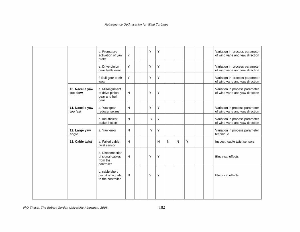
Maintenance Optimisation for Wind Turbines
PhD Thesis, The Robert Gordon University Aberdeen, 2008. 182
d. Premature activation of yaw brake
Y
Y
Y
Variation in process parameter of wind vane and yaw direction
e. Drive pinion gear teeth wear
Y
Y
Y
Variation in process parameter of wind vane and yaw direction
f. Bull gear teeth wear
Y
Y
Y
Variation in process parameter of wind vane and yaw direction
10. Nacelle yaw too slow
a. Misalignment of drive pinion gear and bull gear
N
Y
Y
Variation in process parameter of wind vane and yaw direction
a. Yaw gear reducer seizes
N
Y
Y
Variation in process parameter of wind vane and yaw direction
11. Nacelle yaw too fast
b. Insufficient brake friction
N
Y
Y
Variation in process parameter of wind vane and yaw direction
12. Large yaw angle
a. Yaw error
N
Y
Y
Variation in process parameter technique
a. Failed cable twist sensor
N
N
N
N
Y
Inspect cable twist sensors
b. Disconnection of signal cables from the controller
N
Y
Y
Electrical effects
13. Cable twist
c. cable short circuit of signals to the controller
N
Y
Y
Electrical effects

Maintenance Optimisation for Wind Turbines
PhD Thesis, The Robert Gordon University Aberdeen, 2008. 183
a. Faulty electrical wiring in anemometer
N
Y
Y
Variation in process parameter technique
b. Defective bearing in anemometer
N
Y
Y
Variation in process parameter technique
c. Anemometer deteriorating due to long term exposure to climatic extremes
N
Y
Y
Variation in process parameter technique
14. Wind speed measurement error
d. Anemometer not suitable for application
N
Y
Y
Variation in process parameter technique
a. Potentiometer wind vane deteriorating due to long term exposure to climatic extremes
N
Y
Y
Variation in process parameter technique
15. Wind direction measurement error
b. Potentiometer wind vane not suitable for application
N
Y
Y
Variation in process parameter technique
a. Barometric pressure sensor deteriorating due to long term exposure to climatic extremes
N
Y
Y
Variation in process parameter technique
16. Air density measurement error
b. Barometric pressure sensor not suitable for application
N
Y
Y
Variation in process parameter technique

Maintenance Optimisation for Wind Turbines
PhD Thesis, The Robert Gordon University Aberdeen, 2008. 184
APPENDIX A3 Functional failure C: Over Speeding
System No 1
Facilitator:
SYSTEM: Horizontal Axis Wind Turbine (HAWT) comprising of 3 blades up wind and pitch controlled, 3-stage planetary gearbox, 4-poles asynchronous generator, etc.
Sub-system No
Auditor:
Function: To convert wind kinetic energy into electrical energy within defined speed limit.
Consequence Evaluation
Default action
Functional failures
Failure modes
Failure causes
H
S
E
O
H1 S1 O1 N1
H2 S2 O2 N2
H3 S3 O3 N3
H4
H5
S4
Proposed Task
a. Failed sensors
Y
Y
N
N
N
Y
Inspect controller for failed sensors
b. Disconnection of signal cables to the controller
Y
Y
Y
Thermography
c. Cable short circuit of signals to the controller
Y
Y
Y
Thermography
d. Failed contactors
Y
Y
N
N
N
Y
Inspect controller for failed contactors
e. failed switching relays
Y
Y
N
N
N
Y
Inspect controller for failed switching relays
f. failed fuses
Y
Y
N
N
N
Y
Inspect controller for failed fuses
g. Software design error
Y
Y
Y
Variation in process parameter technique
h. Measurement error
Y
Y
Y
Variation in process parameter technique
C. OVER SPEEDING
1. Controller failure
i. Lightening strike
Y
Y
N
N
N
Y
Inspect lightening protection devices

Maintenance Optimisation for Wind Turbines
PhD Thesis, The Robert Gordon University Aberdeen, 2008. 185
a. Contaminated hydraulic oil13
N
Y
Y
Hydraulic oil analysis
b. Wrong oil viscosity
N
Y
Y
Hydraulic oil analysis
c. High hydraulic fluid temperature
N
Y
Y
Temperature measurement of hydraulic oil
d. Hydraulic pump failure
N
Y
Y
Variation in process parameter technique- pressure measurement
e. Hydraulic cylinder failure
N
Y
Y
Variation in process parameter technique- pressure measurement
f. Hydraulic valve failure
N
Y
Y
Variation in process parameter technique- pressure measurement
g. Faulty circuit protection devices.
N
Y
Y
Tribology
h. Hydraulic seal failure
N
Y
Y
Tribology
i. Hydraulic hose failure
N
Y
Y
Tribology
2. Hydraulic system failure
j. Operating beyond filters life
N
Y
N
N
Y
Replace filters
2c. High hydraulic fluid temperature
a. Failed cooling system
N
Y
Y
Temperature measurement of hydraulic oil
2f.Hydraulic valve failure
a. Cavitations14
N
Y
Y
Variation in process parameter – pressure measurement
212 13 Contaminants include solid particles, air, water or any matter that impairs the function of the fluid 14 Cavitations occur when the volume of hydraulic fluid demanded by any part of a hydraulic circuit exceeds the volume of fluid being supplied.

Maintenance Optimisation for Wind Turbines
PhD Thesis, The Robert Gordon University Aberdeen, 2008. 186
b. High temperature
N
Y
Y
Temperature measurement of hydraulic oil
a. Improper installation
N
Y
Y
Tribology
b. Hydraulic system
contamination
N
Y
Y
Tribology
c. chemical break down of the seal
N
Y
Y
Tribology
2h. Hydraulic seal failure
d. Heat degradation
N
Y
N
N
Y
Replace seal
a. External damage through pulling, kinking, crushing or abrasion of the hose.
N
Y
N
N
N
Y
Inspect hydraulic hoses for damages
b. Multi plane bending
N
Y
N
N
N
Y
Inspect hoses for damages
2j Hydraulic hose failure
c. Temperature extremes
N
Y
Y
Temperature measurement of hydraulic oil
a. Pitching bearings seizes
Y
Y
Y
Acceleration measurement in relation to pitch angle and rotor position
b. Disconnection of pitch angle signal to the controller
Y
Y
Y
Acceleration measurement in relation to pitch angle and rotor position
c. Disconnection of hydraulic pump signal cables from the controller
Y
Y
Y
Acceleration measurement in relation to pitch angle and rotor position
3. Pitching system failure
d. Cable short circuit of signals to the controller
Y
Y
Y
Acceleration measurement in relation to pitch angle and rotor position

Maintenance Optimisation for Wind Turbines
PhD Thesis, The Robert Gordon University Aberdeen, 2008. 187
e. Slip-ring fails
Y
Y
Y
Acceleration measurement in relation to pitch angle and rotor position
a. Fatigue deterioration
N
Y
Y
Vibration monitoring of pitch bearing
b. Misalignment
N
Y
Y
Vibration monitoring of pitch bearing
c. Lack of lubricant
N
Y
Y
Vibration monitoring of pitch bearing
d. Contaminated lubricant
N
Y
Y
Vibration monitoring of pitch bearing
e. wrong lubricant
N
Y
Y
Vibration monitoring of pitch bearing
3a. Pitching bearing seizes
f. Fitting error
N
Y
Y
Vibration monitoring of pitch bearing
a. Insufficient friction
N
Y
N
N
N
Y
Inspect mechanical braking system
4. Mechanical brake failure
b. Too much friction
N
Y
N
N
N
Y
Inspect mechanical braking system
a. Too much wear of brake pads and shoes
N
Y
N
N
Y
Change mechanical brake pad and shoes
b. Too little pretension of spring in calliper
N
Y
Y
Variation in performance parameter technique
c. Spring in calliper broken
N
Y
Y
Variation in performance parameter technique
4a. Insufficient mechanical brake friction
d. Degraded hydraulic oil
N
Y
N
N
Y
Change hydraulic oil

Maintenance Optimisation for Wind Turbines
PhD Thesis, The Robert Gordon University Aberdeen, 2008. 188
e. Too much wear of brake disc
N
Y
N
N
Y
Replace mechanical brake disc
f. Malfunctioning of combination valve
N
Y
Y
Variation in performance parameter technique
g. Leakage in the brake system
N
Y
N
N
N
Y
Inspect braking system for leakage
a. Brake shoes stuck
N
Y
Y
Variation in performance parameter technique
4b. Too much friction
b. Too much pretension of spring in calliper
N
Y
Y
Variation in performance parameter technique
a. Power line fails
Y
Y
Y
Controller fail safe
5. Grid connection failure
b. Disconnection of generator while turbine is in operation
Y
Y
Y
Controller fail safe

Maintenance Optimisation for Wind Turbines
PhD Thesis, The Robert Gordon University Aberdeen, 2008. 189
APPENDIX B
GLOSSARY
*A = Best alternatives
CRA = Annual cost reservation
CBMAC =Annual condition based
servicing of drive train ALCA= Asset Life Cycle Analysis
cmAM =Annual maintenance cost of
condition monitoring AM =Asset Management AMOR= Applied Mathematics & Operational Research BTC= Benefit- to-cost ratio BS= British Standard CBM = Condition Based Maintenance
MTC = Cost of material
LdC = Cost of loading
OldC = Cost of offloading
TPC = Cost of transportation
CRC = Cost of crane hire per day
(including cost of driver, mobilisation and demobilisation fee)
EHC = Cost of energy per kWh
fC = Capacity factor
cmC = Capital cost of condition
monitoring system CBM = Condition Based Maintenance CREST= Centre for Renewable Energy Systems Technology CTA= Critical Task Analysis DTMM = Delay Time Maintenance Model d = Discount rate (% /100) ECN = Energy Centre Netherlands ETA= Event Tree Analysis ESI = Electricity Supply Industry
EWTCG= European Wind Turbine Certification Guidelines F =Failure
cF = Failure consequences
FBM = Failure Based Maintenance FMEA= Failure Mode and Effect Analysis FTA=Fault Tree Analysis
( )TF =Cumulative Distribution Function
)(Tf = Probability Density Function GRP= Glass fibre Reinforced Plastic GSN = Generator Serial Number HAZAN= HAZard ANalysis HAZOP= HAZard OPeratibility HSE= Health, Safety and Environment HSS =High Speed Shaft i= Alternative IAM =Institute of Asset Management IMS =InterMediary speed Shaft IEC = International Electro-Technical Commission KPM = Key Performance Measurement KPI = Key Performance Indicator LCC = Life Cycle Cost
RTL = Labour rate per hour
hcL = Lead time to hire a crane
m= Decision criteria MTBF =Mean Time Between Failure MTTF =Mean Time To Failure MTTR=Mean Time To Repair MLE = Maximum Likelihood Estimation MSF= Modelling Systems Failure MW = Mega Watt n= Number of competing alternatives
PnN = Number of person

Maintenance Optimisation for Wind Turbines
PhD Thesis, The Robert Gordon University Aberdeen, 2008. 190
dyN = Number of working days
TN = Number of turbines in a wind farm
CBMNPV = Net present Value of
Condition Based Maintenance
TBMNPV = Net present Value of Time Based Maintenance OEM = Original Equipment Manufacturer
GO & = Oil &Gas MO & = Operation &Maintenance
IntervalFP − =P is point where defect can be identified and F point where component fails PM =Preventive Maintenance PW = Present worth PWA= Present worth per annum QRA= Quantified Risk Assessment QMO= Quantitative Maintenance Optimisation
dyR = Replacement days including
travel time RAM = Reliability Availability and Maintainability RBI = Risk Based Inspection RBD= Reliability Block Diagram RCM = Reliability Centred Maintenance RCA= Root Cause Analysis RPM = Revolution Per Minute RO = Renewable Obligation order ROC = Renewable Obligation Certificate S = Suspension
iS = Total score of alternative
ijS = Alternative ratings
SCADA = Supervisory Control and Data Acquisition SCIG= Squirrel Cage Induction Generator SWIFT= Structured What IF Technique
T = Time
CITA = Total annual cost of inspection
TBM = Time Based Maintenance TPM = Total Productive Maintenance
PLT = Total Production loss
LBTC = Total cost of labour
ASTC = Total cost of access
MTTC = Total cost of material T = Analysis period
ATV = Value added tax
jW = Criterion weight
hrW = Work hours per day
WE= Weighted Evaluation WSI= Water Supply Industry WT = Wind Turbine WF = Wind Farm
PRWT = Wind turbine power rating in kilowatt (kW) α = Defects rate β = Shape Parameter of the Weibull distribution η = Scale Parameter of the Weibull distribution ϕ = Failure rate
γ1
= Delay time
∆ = Inspection Interval ∗∆ = Optimal Inspection Interval

Maintenance Optimisation for Wind Turbines
PhD Thesis, The Robert Gordon University Aberdeen, 2008. 191
APPENDIX C
ABSTRACTS OF PUBLISHED PAPERS Three (3) journal and three (3) conference papers have been published as a result of the
research work that underpins this thesis. Also, two (2) additional papers have been
written and are currently under review for journals publication. Abstracts of the six (6)
published papers are presented as follows:
C.1 ASSET MANAGEMENT PROCESSES IN THE WIND ENERGY INDUSTRY
Jesse A Andrawus, John Watson and Mohammed Kishk
Proceedings of the 2nd Joint International Conference on “Sustainable Energy and
Environment (SEE 2006)” 21-23 November 2006, Bangkok, Thailand, 269-274.
Asset management (AM) has evolved from several industrial sectors to
describe holistic application of business best practices to satisfy all
stakeholders’ requirements. The processes, tools and techniques of AM
are currently well-established in the mature industries. On the other
hand, wind is becoming an increasingly important source of energy for
countries that ratify to reduce emission of greenhouse gases and mitigate
global warming. This creates a huge investment potential for the wind
energy industry with a wide range of possible stakeholders. However,
achieving return on investment in wind farms is affected by interrelated
stakeholders’ requirements and assets technical issues. These require a
well-founded Asset Management (AM) frame-work currently lacking in
the wind industry. The main objective of this paper is to identify and
transform crucial requirements for effective management of wind farms
into AM processes as a first step towards developing a structured model
for AM in the wind energy industry. Six fundamental processes are
determined and presented with a detailed explanation.

Maintenance Optimisation for Wind Turbines
PhD Thesis, The Robert Gordon University Aberdeen, 2008. 192
Keywords: Asset Management, Wind Energy, Business Values, Process
modelling.
C.2 DETERMINING AN APPROPRIATE CONDITION-BASED MAINTENANCE STRATEGY FOR WIND TURBINES
Jesse A Andrawus, John Watson, Mohammed Kishk and Allan Adam
Proceedings of the 2nd Joint International Conference on “Sustainable Energy and
Environment (SEE 2006)” 21-23 November 2006, Bangkok, Thailand, 275-280.
Maintenance is fundamental to effective management of wind farms due
to its impact on productivity of wind turbines, operational costs and
hence revenue generation. Essentially, there are two common
maintenance strategies applied to wind turbines; Time-Based
Maintenance (TBM) which involves carrying out tasks at predetermined
regular-intervals and Failure-Based Maintenance (FBM) which involves
using a wind turbine until it fails. However, the impact of failure
consequences on revenue generation and electricity network limit the
adequacy of these strategies to support the current commercial drivers of
the wind industry. Reliability-Centred Maintenance (RCM) is a technique
mostly used to select suitable maintenance strategies for physical assets.
In this paper, the approach of RCM is applied to Horizontal Axis Wind
Turbines to identify possible failure modes, causes and the resultant
effects on system operation. Suitable Conditioned Based Maintenance
(CBM) activities are identified.
Keywords: Wind turbines, Reliability-Centred Maintenance, Condition-
Based Maintenance.

Maintenance Optimisation for Wind Turbines
PhD Thesis, The Robert Gordon University Aberdeen, 2008. 193
C.3 THE SELECTION OF A SUITABLE MAINTENANCE
STRATEGY FOR WIND TURBINES
Jesse A. Andrawus, John Watson, Mohammed Kishk and Allan Adam
International Journal of Wind Engineering, 2006, Vol 30 No 6, pp. 471-486.
Common maintenance strategies applied to wind turbines include ‘Time-
Based’ which involves carrying out maintenance tasks at predetermined
regular-intervals and ‘Failure-Based’ which entails using a wind turbine
until it fails. However, the consequence of failure of critical components
limits the adequacy of these strategies to support the current commercial
drivers of the wind industry. Reliability-Centred Maintenance (RCM) is a
technique used mostly to select appropriate maintenance strategies for
physical assets. In this paper, a hybrid of an RCM approach and Asset
Life-Cycle Analysis technique is applied to Horizontal-Axis Wind
Turbines to identify possible failure modes, causes and the resultant
effects on system operation. The failure consequences of critical
components are evaluated and expressed in financial terms. Suitable
Condition-Based Maintenance activities are identified and assessed over
the life-cycle of wind turbines to maximise the return on investment in
wind farms.
Keywords: Wind turbines, Reliability-Centred Maintenance, Failure
Mode and Effect Analysis, Asset Life-cycle Analysis, Condition-Based
Maintenance.

Maintenance Optimisation for Wind Turbines
PhD Thesis, The Robert Gordon University Aberdeen, 2008. 194
C.4 WIND TURBINE MAINTENANCE OPTIMISATION:
PRINCIPLES OF QUANTITATIVE MAINTENANCE
OPTIMISATION
Jesse A. Andrawus, John Watson and Mohammed Kishk International Journal of Wind Engineering, 2007, Vol 31 No 2, pp. 101-110.
Maintenance optimisation is a crucial issue for industries that utilise
physical assets due to its impact on costs, risks and performance. Current
quantitative maintenance optimisation techniques include Modelling
System Failures MSF (using Monte Carlo simulation) and Delay-Time
Maintenance Model (DTMM). The MSF investigates equipment failure
patterns by using failure distribution, resource availability and spare-
holdings to determine optimum maintenance requirements. The DTMM
approach examines equipment failure patterns by considering failure
consequences, inspection costs and the period to determine optimum
inspection intervals. This paper discusses the concept, relevance and
applicability of the MSF and DTMM techniques to the wind energy
industry. Institutional consideration as well as the benefits of practical
implementation of the techniques are highlighted and discussed.
Keywords: Wind turbine, Maintenance optimisation, Modelling System
Failures, Monte Carlo Simulation, Delay-time maintenance model.

Maintenance Optimisation for Wind Turbines
PhD Thesis, The Robert Gordon University Aberdeen, 2008. 195
C.5 MAINTENANCE OPTIMISATION OF WIND TURBINES:
LESSONS FOR THE BUILT ENVIRONMENT
Jesse A. Andrawus, John Watson and Mohammed Kishk
Proceedings 23rd Annual ARCOM Conference, 3-5 September 2007, Belfast, UK,
Association of Researchers in Construction Management, 893-902.
Maintenance optimisation is indispensable to the core business objectives
of industries that utilises physical assets. A quantitative maintenance
optimisation technique known as the Modelling System Failures (MSF)
is critically reviewed to identify its relevance to industries that employs
physical assets. Practical application of the approach to optimise the
maintenance activities of wind turbines is explored and discussed in a
case study. The analysis is based maximum likelihood parameter
estimation in the Weibull distribution. Shape and scale parameters for a
gearbox and its components are estimated. The estimated parameters are
used to design Reliability Block Diagrams to model the failures of the
gearbox of a selected wind turbine. The models are simulated using
Monte Carlo simulation software to assess the reliability, availability and
maintainability of the gearbox, and the resultant effects on the wind
turbine operation. The methodology presented in the paper is sufficiently
generic to any mechanical system in the Built Environment/Construction
Industry.
Keywords: Wind Turbine, Maintenance Optimisation, Monte Carlo
Simulation, Reliability Block Diagrams.

Maintenance Optimisation for Wind Turbines
PhD Thesis, The Robert Gordon University Aberdeen, 2008. 196
C.6 MODELLING SYSTEM FAILURES TO OPTIMISE WIND
TURBINE MAINTENANCE
Jesse A. Andrawus, John Watson and Mohammed Kishk International Journal of Wind Engineering, 2007, Vol 31 No 6, pp. 503-522.
Modelling System Failures (MSF) is a unique quantitative maintenance
optimisation technique which permits the evaluation of life-data samples and
enables the design and simulation of the system’s model to determine optimum
maintenance activities. In this paper, the approach of MSF is used to assess the
failure characteristics of a horizontal axis wind turbine. Field failure data are
collated and analysed using the Maximum Likelihood Estimation in the Weibull
Distribution; hence shape (β) and scale (η) parameters are estimated for critical
components and subsystems of the wind turbine. Reliability Block Diagrams are
designed to model the failures of the wind turbine and of a selected wind farm.
The models are simulated to assess the reliability, availability and
maintainability of the wind turbine and the farm; taking into account the costs
and availability of maintenance crew and spares holding. Optimal maintenance
activities are determined to minimise the total life-cycle cost of the wind farm.
Key words: Wind turbine, Failure Modelling, Reliability, Availability and
Maintenance Optimisation