Make Trade not War?∗

Philippe Martin† Thierry Mayer‡ Mathias Thoenig§

April 12, 2006

Abstract

This paper analyzes theoretically and empirically the relationship between military conflictsand trade. We show that the intuition that trade promotes peace is only partially true even in amodel where trade is beneficial to all, military conflicts reduce trade and leaders take into accountthe benefits of peace. When war can occur because of the presence of asymmetric information, theprobability of escalation is lower for countries that trade more bilaterally because of the opportunitycost associated with the loss of trade gains. However, countries more open to global trade have ahigher probability of war because multilateral trade openness decreases bilateral dependence to anygiven country. We test our predictions on a large data set of military conflicts on the 1950-2000period. Using different strategies to solve the endogeneity issues, including instrumental variables,we find robust evidence for the contrasting effects of bilateral and multilateral trade openness.

JEL classification: F12, F15Keywords: Globalization, Trade, War.

∗We thank Daron Acemoglu, Harry Bowen, Martin Feldstein, Gregory Hess, Philippe Jehiel, Ethan Kapstein, SolomonPolachek, Robert Powell and Andy Rose for very helpful comments. We also thank participants during presentationsat the NBER Summer Institute, ERWIT (Rotterdam), the CEPR “Macroeconomics and war” conference (Barcelona),and seminars in Berkeley, UC Davis, Tel-Aviv, Jerusalem, Georgetown, LSE, Geneva, Stockholm, Cergy, Paris, IUE-Florence, INSEAD, UNCTAD, IMF, WTO, and New York Fed. Kimberly Ann Elliot kindly provided us the data ontrade sanctions. All errors remain ours. Philippe Martin thanks Cepremap for financial assistance.

†University of Paris 1 Pantheon-Sorbonne (CES), PSE and CEPR‡University of Paris-Sud, CEPII, PSE and CEPR§University of Geneva, PSE and CEPR

1 Introduction

“The natural effect of trade is to bring about peace. Two nations which trade together, render them-selves reciprocally dependent; for if one has an interest in buying, the other has an interest in selling;and all unions are based upon mutual needs.”

Montesquieu, De l’esprit des Lois, 1758.

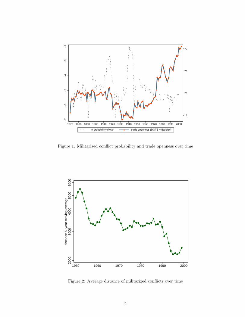
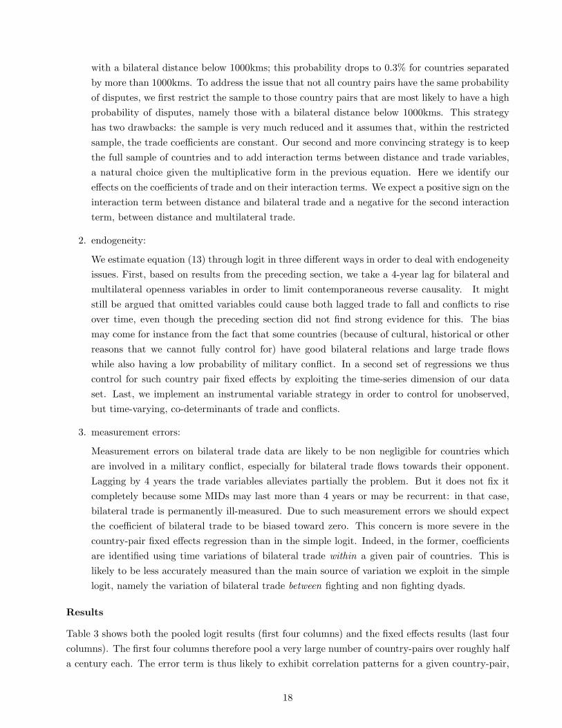
Does globalization pacify international relations? The “liberal” view in political science arguesthat increasing trade flows, and the spread of free markets and democracy should limit the incentiveto use military force in interstate relations. This vision, which can partly be traced back to Kant’sEssay on Perpetual Peace (1795), has been very influential: the main objective of the Europeantrade integration process was to prevent the killing and destruction of the two World Wars from everhappening again1. Figure 1 suggests 2 however that on the 1870-2001 period, the correlation betweentrade openness and military conflicts is not a clear cut one. The first era of globalization, at the end ofthe XIXth century, was a period of rising trade openness and of multiple military conflicts, culminatingwith World War I. Then, the interwar period was characterized by a simultaneous collapse of worldtrade and conflicts. After World War II, world trade increased rapidly while the number of conflictsdecreased (although the risk of a global conflict was obviously high). There is no clear evidence thatthe 1990s, during which trade flows increased dramatically, was a period of lower prevalence of militaryconflicts even taking into account the increase in the number of sovereign states.

The objective of this paper is to shed light on the following question: if trade promotes peace asillustrated by the European example, why is it that globalization, interpreted as trade liberalizationat the global level, has not lived up to its promise of decreasing the prevalence of violent interstateconflicts? We offer a theoretical and empirical answer to this question. On the theoretical side, we builda framework where escalation to military conflicts may occur because of the failure of negotiations ina bargaining game. The structure of this game is fairly general: (i) war is Pareto dominated by peace;(ii) countries have private information on what happens in case of war; (iii) we impose no institutionalconstraint so that countries can choose any type of negotiation protocol. We then embed this gamein a standard new trade theory model with trade costs. We show that a pair of countries with morebilateral trade has a lower probability of bilateral war. However, multilateral trade openness has theopposite effect: any pair of countries more open with the rest of the world decreases its degree ofbilateral dependence and this results in a higher probability of bilateral war. A theoretical predictionof our model is that globalization of trade flows changes the nature of conflicts. It decreases theprobability of global conflicts (maybe the most costly in terms of human welfare) but increases the

1Before this, the 1860 Anglo-French commercial Treaty was signed to diffuse tensions between the two countries.Outside Europe, MERCOSUR was created in 1991 in part to curtail the military power in Argentina and Brazil, thentwo recent and fragile democracies with potential conflicts over natural resources.

2Figure 1 depicts the occurrence of Militarized Interstate Disputes (MID) between country pairs divided by the totalnumber of countries. MIDs range from level 1 to 5 in terms of hostility level. Figure 1 accounts for level 3 (display offorce), level 4 (use of force) and 5 (war, which requires at least 1000 death of military personnel). See section 3.1 for amore precise description of the data. Trade openness is the sum of world trade (exports and imports) divided by worldGDP (trade data comes from the IMF DOTS dataset and Barbieri, 2002, while GDP figures come from World Bank’sWDI, and Maddison, 2001, for historical data).

1

.1.2

.3.4

−7

−6

−5

−4

−3

−2

1870 1880 1890 1900 1910 1920 1930 1940 1950 1960 1970 1980 1990 2000

ln probability of war trade openness (DOTS + Barbieri)

Figure 1: Militarized conflict probability and trade openness over time

2000

3000

4000

5000

6000

dist

ance

5−

year

mov

ing

aver

age

1950 1960 1970 1980 1990 2000

Figure 2: Average distance of militarized conflicts over time

2

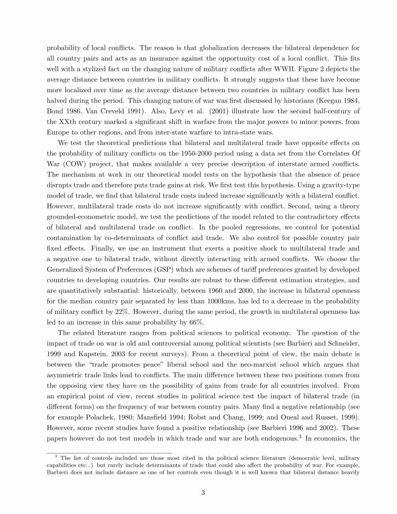
probability of local conflicts. The reason is that globalization decreases the bilateral dependence forall country pairs and acts as an insurance against the opportunity cost of a local conflict. This fitswell with a stylized fact on the changing nature of military conflicts after WWII. Figure 2 depicts theaverage distance between countries in military conflicts. It strongly suggests that these have becomemore localized over time as the average distance between two countries in military conflict has beenhalved during the period. This changing nature of war was first discussed by historians (Keegan 1984,Bond 1986, Van Creveld 1991). Also, Levy et al. (2001) illustrate how the second half-century ofthe XXth century marked a significant shift in warfare from the major powers to minor powers, fromEurope to other regions, and from inter-state warfare to intra-state wars.

We test the theoretical predictions that bilateral and multilateral trade have opposite effects onthe probability of military conflicts on the 1950-2000 period using a data set from the Correlates OfWar (COW) project, that makes available a very precise description of interstate armed conflicts.The mechanism at work in our theoretical model rests on the hypothesis that the absence of peacedisrupts trade and therefore puts trade gains at risk. We first test this hypothesis. Using a gravity-typemodel of trade, we find that bilateral trade costs indeed increase significantly with a bilateral conflict.However, multilateral trade costs do not increase significantly with conflict. Second, using a theorygrounded-econometric model, we test the predictions of the model related to the contradictory effectsof bilateral and multilateral trade on conflict. In the pooled regressions, we control for potentialcontamination by co-determinants of conflict and trade. We also control for possible country pairfixed effects. Finally, we use an instrument that exerts a positive shock to multilateral trade anda negative one to bilateral trade, without directly interacting with armed conflicts. We choose theGeneralized System of Preferences (GSP) which are schemes of tariff preferences granted by developedcountries to developing countries. Our results are robust to these different estimation strategies, andare quantitatively substantial: historically, between 1960 and 2000, the increase in bilateral opennessfor the median country pair separated by less than 1000kms, has led to a decrease in the probabilityof military conflict by 22%. However, during the same period, the growth in multilateral openness hasled to an increase in this same probability by 66%.

The related literature ranges from political sciences to political economy. The question of theimpact of trade on war is old and controversial among political scientists (see Barbieri and Schneider,1999 and Kapstein, 2003 for recent surveys). From a theoretical point of view, the main debate isbetween the “trade promotes peace” liberal school and the neo-marxist school which argues thatasymmetric trade links lead to conflicts. The main difference between these two positions comes fromthe opposing view they have on the possibility of gains from trade for all countries involved. Froman empirical point of view, recent studies in political science test the impact of bilateral trade (indifferent forms) on the frequency of war between country pairs. Many find a negative relationship (seefor example Polachek, 1980; Mansfield 1994; Robst and Chang, 1999; and Oneal and Russet, 1999).However, some recent studies have found a positive relationship (see Barbieri 1996 and 2002). Thesepapers however do not test models in which trade and war are both endogenous.3 In economics, the

3 The list of controls included are those most cited in the political science literature (democratic level, militarycapabilities etc...) but rarely include determinants of trade that could also affect the probability of war. For example,Barbieri does not include distance as one of her controls even though it is well known that bilateral distance heavily

3

only comparable empirical paper on the issue is a recent paper by Glick and Taylor (2005) whichfocuses on the reverse causal link, i.e. on the effect of war on trade. They control for the standarddeterminants of trade as used in the gravity equation literature. To our knowledge, our paper ishowever the first to derive theoretically the two-sided effect of trade on peace (positive for bilateraltrade and negative for multilateral trade) and to empirically test this prediction.

Skaperdas and Syropoulos (2001 and 2002) show in a theoretical model that terms of trade effectsmay intensify conflict over resources, a mechanism from which we abstract in our model. We alsoabstract from internal conflicts between factors of production that may be generated by opening totrade as in Schneider and Schulze (2005). The recent literature on the number and size of countries(see Alesina and Spolaore, 1997 and 2003) has also clear connections with our paper because in bothframeworks, a key mechanism is that globalization reduces local economic dependence. In Alesina andSpolaore, the consequence is an increase in the equilibrium number of countries. In our framework, itdecreases the opportunity cost of conflict and increases the equilibrium number of local wars. Alesinaand Spolaore (2005 and 2006) also study the link between conflicts, defense spending and the numberof countries. Their model aims to explain how a decrease in international conflicts can be associatedwith an increase in localized conflicts between a higher number of smaller countries. Their explanationis the following: when international conflicts become less frequent, the advantages of large countries(in terms of provision of public and defense goods) weaken so that countries split and the number ofcountries increases. This itself leads to an increase in the number of (localized) conflicts. In our paper,the number and size of countries are exogenous but trade and the probability of escalation to war areendogenous.

The next section derives the theoretical probability of escalation to war between two countries asa function of the degree of asymmetric information, bilateral and multilateral trade and analyzes theambivalent role of trade on peace. The third section first quantifies the impact of war on both bilateraland multilateral trade and then tests the impact of trade openness, bilateral and multilateral, on theprobability of military conflicts between countries.

2 The theory

In this section, we analyze a simple model of negotiation and escalation to war. We then embed it ina model of trade to assess the marginal impact of trade on war.

2.1 Escalation to war under asymmetric information

We follow the rationalist view of war among political scientists (see Fearon 1995 and Powell, 1999 forsurveys) and economists (see Grossman, 2003) whose aim is to explain the puzzle that wars do occurdespite their costs, even in the presence of rational leaders. The rationalist view is the most naturalstructure for our argument because trade gains are then taken into account in the decision to go towar.4

affects bilateral trade. Distance also affects negatively the probability of conflicts (see Kocs, 1995).4Scholars in political sciences have developed two alternative arguments: i) agents (and states leaders) may be

irrational and misperceive the costs of war; ii) leaders may be those who enjoy the benefits of war while the costs are

4

Studies in the rationalist view of war however greatly differ with respect to their assumptions oninstitutional setting and the negotiations protocols. In this paper, the only institutional constraintwe impose is that the negotiation protocol (bilateral or multilateral negotiations, repeated stages...)chosen is the one that maximizes the ex-ante welfare of both countries. This more general view has twoadvantages. First, it avoids the main drawback of the existing literature, namely the high sensitivityof results to the underlying restrictions made on institutions. Second, it is fully consistent with therationalist school view of war, as rationality implies that leaders choose the most efficient institutionalsetting and negotiation protocol.

Consider two countries i and j. Exogenous disputes may arise between these two countries. Disputescan end peacefully if countries succeed through a negotiated settlement or can escalate into militaryconflict if negotiations fail. The timing of the game is the following: if a dispute arises, a negotiationprotocol is optimally chosen, then information is privately revealed and negotiations take place. Waroccurs or does not depending on the outcome of negotiations. Production, trade and consumption arethen realized as described in the next section.

Leaders in both countries care about the utility level of a representative agent of their own countrywho, in peace, obtains respectively: (UP

i , UPj ). In a situation of war, they obtain a stochastic outside

option (UWi , UW

j ). Peace Pareto-dominates war so that the gains of the winning country are lowerthan the losses of the defeated country:

SP ≡ UPi + UP

j > UWi + UW

j ≡ SW (1)

Escalation to war is avoided whenever countries i and j agree on a sharing rule of SP . We assumethat stochastic outside options (UW

i , UWj ) are equal on average to the equilibrium values (UW

i , UWj )

as determined in the next section. More precisely:

UWi = (1 + ui)UW

i and UWj = (1 + uj)UW

j (2)

where ui and uj are privately known by each country. This private information could for instanceinclude the actual strength of national military forces. Unconditional mean and variance are: E(ui) =E(uj) = 0 and var(ui) = var(uj) = V 2/8. Hence, the parameter V measures the degree of informationalasymmetry between the countries.

Solving for the second best protocol in bargaining under private information constitutes one of themost celebrated results in the mechanism design literature (Myerson and Satherwaite 1983). However,we cannot apply directly Myerson and Satherwaite’s results because they assume that 1) once anagent has agreed to participate in the negotiation, it has no further right to quit the negotiation table;2)private information should be independently distributed between agents. Hereafter, we relax both

suffered by other agents (citizens and soldiers). We ignore those alternative explanations of war because it is unlikely thatthe trade openness channel interacts with them. Indeed an irrational leader may decide to go to war whatever the tradeloss suffered by his country. Similarly, the way the trade surplus (and the trade loss in case of conflict) is shared betweenpolitical leaders and the rest of the population is not obvious. Hence, marginally, a larger level of trade openness hasno clear cut impact on the trade-off between the marginal benefits of war enjoyed by political leaders and the marginalcosts suffered by the population. Consequently, internal politics do not play a role in our theoretical analysis. Studieson the relationship between domestic politics and war include Garfinkel (1994) and Hess and Orphanides (1995, 2001).

5

MA

MB

M A

B

A’

B’

Ui

Uj

Average outside option

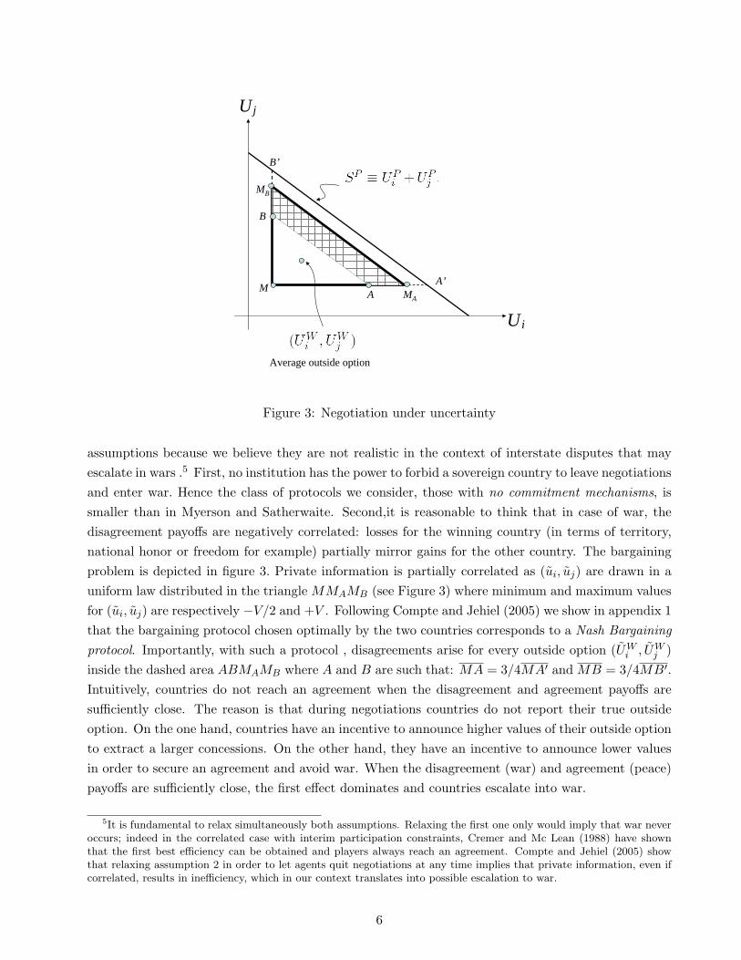
Figure 3: Negotiation under uncertainty

assumptions because we believe they are not realistic in the context of interstate disputes that mayescalate in wars .5 First, no institution has the power to forbid a sovereign country to leave negotiationsand enter war. Hence the class of protocols we consider, those with no commitment mechanisms, issmaller than in Myerson and Satherwaite. Second,it is reasonable to think that in case of war, thedisagreement payoffs are negatively correlated: losses for the winning country (in terms of territory,national honor or freedom for example) partially mirror gains for the other country. The bargainingproblem is depicted in figure 3. Private information is partially correlated as (ui, uj) are drawn in auniform law distributed in the triangle MMAMB (see Figure 3) where minimum and maximum valuesfor (ui, uj) are respectively −V/2 and +V . Following Compte and Jehiel (2005) we show in appendix 1that the bargaining protocol chosen optimally by the two countries corresponds to a Nash Bargainingprotocol. Importantly, with such a protocol , disagreements arise for every outside option (UW

i , UWj )

inside the dashed area ABMAMB where A and B are such that: MA = 3/4MA′ and MB = 3/4MB′.

Intuitively, countries do not reach an agreement when the disagreement and agreement payoffs aresufficiently close. The reason is that during negotiations countries do not report their true outsideoption. On the one hand, countries have an incentive to announce higher values of their outside optionto extract a larger concessions. On the other hand, they have an incentive to announce lower valuesin order to secure an agreement and avoid war. When the disagreement (war) and agreement (peace)payoffs are sufficiently close, the first effect dominates and countries escalate into war.

5It is fundamental to relax simultaneously both assumptions. Relaxing the first one only would imply that war neveroccurs; indeed in the correlated case with interim participation constraints, Cremer and Mc Lean (1988) have shownthat the first best efficiency can be obtained and players always reach an agreement. Compte and Jehiel (2005) showthat relaxing assumption 2 in order to let agents quit negotiations at any time implies that private information, even ifcorrelated, results in inefficiency, which in our context translates into possible escalation to war.

6

The probability of escalation to war corresponds to the surface of ABMAMB divided by the surfaceof the triangle MMAMB : Pr(escalationij) = 1 − MAMB

MMAMMB. Assuming that the informational noise

V is not too large, we obtain:

Pr(escalationij) = 1− 14V 2

[(UP

i + UPj

)− (UW

i + UWj )]2

UWi UW

j

(3)

The probability of escalation to war increases with the degree of asymmetric information as measuredhere by the observational noise V 2 and decreases with the difference in the surplus under peace andunder war, i.e. the opportunity cost of war. Trade affects both surpluses as shown in the next section.

2.2 Trade in a multi-country world

Our theoretical framework is based on a standard new trade theory model with trade costs. Thefirst reason we use such a model is that the multiplicity of trade partners is going to allow countriesto diversify the origin of imports and therefore to decrease dependence on a single partner. Thisdiversity effect is a natural feature of the Dixit-Stiglitz monopolistic competition model. Of course,the same results would apply if imperfectly substitutable intermediate goods were required to producea final consumption good. The second reason is that distance between countries plays an importanttheoretical and empirical role for both trade and war and is relatively easy to manipulate in new trademodels. Note that trade is welfare improving for all countries in such a model.

The world consists of R countries which produce differentiated goods under increasing returns.The utility of a representative agent in country i is equal to consumption of a composite good C madeof all varieties produced in the world with the standard Dixit-Stiglitz form:

Ui = Ci =

[R∑

h=1

nhcσ−1

σih

] σσ−1

(4)

where nh is the number of varieties produced in country h, cih is demand in country i for a varietyproduced in country h, and σ > 1 is the elasticity of substitution. Dual to this is the price index foreach country:

Pi =

(R∑

h=1

nh (phTih) 1−σ

)1/(1−σ)

(5)

where ph is the mill price of products made in h, and Tih > 1 represents the usual iceberg trade costs.Those depend on distance and other trade impediments such as political borders or trade restrictions.If one unit of good is exported from country h to country i, only 1/Tih units are consumed. In eachcountry, the different varieties are produced under monopolistic competition and the entry cost in themonopolistic sector requires f units of a freely tradable good which is chosen as numeraire. Producedin perfect competition with labor only, this sector serves to fix the wage rate in country i to its laborproductivity ai, common to both sectors. It is not crucial to our argument but simplifies the analysis.Mill prices in the manufacturing sector in all countries are identical and equal to the usual mark-upover marginal cost (here equal to 1): pi = σ/ (σ − 1) ,∀i. As labor is the only factor of production,

7

and agents are each endowed with one unit of labor, this implies that total expenditure of country i

is Ei = Li where Li ≡ aiLi is effective labor, productivity multiplied by Li the number of workers incountry i. Also, labor market equilibrium and free entry imply ni = Li/(fσ). The value of importsby country i from country j depends on both countries incomes, prices and trade costs:

mij ≡ njpjTijcij = EiEj

(pjTij

Pi

)1−σ

, (6)

a standard gravity equation. Utility increases with trade flows, the number of varieties and decreaseswith trade costs:

Ui =σ − 1

σ

(f

σ

) −1σ−1

[R∑

h=1

n1σh

(mih

Tih

)σ−1σ

] σσ−1

. (7)

We assume that the possible economic effects of a war between country i and country j are: (1)a decrease of λ percent in effective labor Li and Lj in both countries (which may come from a lossin productivity or in factors of production); and (2) an increase of τbil percent and τmulti percent, inrespectively the bilateral and the multilateral trade costs Tij and Tih, h 6= i, j on differentiated goods.During conflicts, borders are closed, transport infrastructures are destroyed and confidence is shaken.These can affect both bilateral and multilateral trade costs. Note that the assumed percentage increasein trade costs due to war is the same across the two fighting countries, but that the level of initialtrade costs between countries differ across country-pairs.

To sum up, a country i’s welfare under peace is UPi = U(xi) where the vector xi ≡ (Li, Lj , Tij , Tih).

Under war, country i’s welfare is stochastic (see equation (2)) but is equal on average to an equilibriumvalue UW

i = U [xi(1−∆)] with: ∆ ≡ (λ, λ,−τbil,−τmulti).

2.3 Trade openness and war

According to our model, the probability of escalation to war between country i and country j is givenby (3). Together with (7), we show in appendix 2 that, using a Taylor expansion around the symmetricequilibrium where countries i and j are identical in size, war occurs with probability:

Pr(escalationij) = 1− 1V 2

[W1λ + W2τbil + W3τmulti]2 (8)

The term in brackets is the total welfare differential between war and peace for both countries. Thisdifferential has three components which are given in appendix 2. The first one, W1 > 0, says that warreduces available resources among belligerents. There is a negative impact on welfare because of thedirect impact on income and the indirect impact on number of varieties consumed (locally producedand imported from j). The second component, W2 > 0, stands for the fact that war potentiallyincreases bilateral trade costs and therefore decreases bilateral trade. Similarly the third componentW3 > 0 stands for the possible increase of multilateral trade costs.

Importantly, equation (8) can also be rewritten in terms of the observable trade patterns. For this,

we use (6) and the national accounting identity:miiEi

+ mij

Ei+

R∑h 6=j,i

mihEi

= 1, where mii is the value of

trade internal to country i and (mij ,mih) are the observable trade flows in final goods. We then obtain

8

the probability of escalation as a function of observable bilateral import flows(

mij

Ei

)and multilateral

import flows

(R∑

h 6=j,i

mihEi

)as ratios of income:

Pr(escalationij) = 1− 1V 2

σλ

σ − 1+ τbil

mij

Ei−(

λ

σ − 1− τmulti

) R∑h 6=j,i

mih

Ei

2

(9)

It brings two important implications which are tested in the empirical section.

Testable implication 1: An increase in bilateral imports of i from j, as a ratio of the importer’sincome decreases the probability of escalation to war between these two countries.

This prediction holds as long as τbil > 0: bilateral trade costs increase following a war between i

and j. We test this condition in the empirical section and find that it holds. If war increases bilateraltrade costs, it lowers trade gains the more so the higher the ex-ante import flows. Hence, observedbilateral trade openness reveal the opportunity cost of a bilateral war.

Testable implication 2: An increase in multilateral imports (from countries other that j) as a ratioof country i’s income, implies a higher probability of escalation to war with country j.

This prediction holds under a stricter condition than the one necessary for testable implication 1,namely that: τmulti < λ

σ−1 , the increase in multilateral trade costs following a war with j is smallenough compared to the welfare loss due to the decrease in the number of varieties consumed thatcomes from the loss in factors of production of i and j. In the empirical section, we find that the impactof military conflicts on multilateral trade costs is indeed either small or insignificant in the post WorldWar II period. In addition, empirical work by Hess (2004) shows that pure economic costs of conflictsare large, which in the context of our model suggests that λ, the percentage decrease in effectivelabor and income, is large. The intuition for testable implication 2 is that a high level of multilateraltrade reduces the bilateral dependence vis-a-vis country j: the welfare loss due to the fall in varietiesfrom i and j is lower when internal trade flows and import flows from j are smaller in proportion oftotal expenditures, that is, when multilateral trade openness is large. Observed multilateral opennesseffectively works like an insurance device in case of war and therefore reduces the opportunity cost ofa bilateral war.

We now discuss the impact of globalization on war. By differentiating equation (8), we obtainthe effect on the probability of escalation of a decrease in bilateral trade barriers Tij . Appendix2 shows that lower bilateral trade costs between i and j decreases the probability of escalation towar between these two countries: d Pr(escalationij)

d(−Tij)< 0. A sufficient condition for this result to hold

is τmulti < λσ−1 . The intuition is similar to Testable implication 1. Under the same condition, an

increase in multilateral trade openness of country i with other countries than country j implies ahigher probability of escalation to war with country j: d Pr(escalationij)

d(−Tih) > 0.A direct consequence of these two results is that regional and multilateral trade liberalization

may have very different implications for the prevalence of war. Regional trade agreements between a

9

group of countries will unambiguously lead to lower prevalence of regional conflicts. Multilateral tradeliberalization may increase the prevalence of bilateral conflicts.

We can use our model to shed light on the following question: why has the process of globalizationnot led to a decrease of the number of military conflicts as was hoped in the beginning of the 1990s?For simplicity, we assume that the world is made of R similar countries with symmetric trade barriers,Tij = T for all i, j. We interpret globalization as a uniform decrease in trade barriers between allcountry pairs.

Result 1: Globalization – interpreted as a symmetric decrease in trade costs – increases the prob-ability of war between all country pairs

(d Pr(escalationij)

d(−T ) > 0)

if[

λσ−1 − τmulti

](R − 2) > τbil (see

appendix 2 for proof).

This result holds when the increase in multilateral trade costs (τmulti) following a bilateral conflictis low and when the number of countries (R) is sufficiently large. The reason is that in a worldwhere countries have a very diverse set of trade partners, globalization reduces the bilateral economicdependence and the opportunity cost of war for all pairs of countries. The intuition that trade is goodfor peace can actually be reversed. There are two important provisos to this (pessimistic) message.The first crucial proviso is that multilateral trade liberalization changes the nature of war: it increasesthe probability of small scale wars but it decreases the probability of a large scale war. R is the numberof countries in the model, but can also be interpreted as the number of coalitions with a dispute thatmay or may not escalate into a war. In the limit, when R = 2, globalization unambiguously decreasesthe probability of a world war between two coalitions of countries for the same reason that bilateraltrade liberalization induces a lower probability of bilateral war. If one thinks that world wars are themost costly in terms of human welfare, then globalization plays a very positive role.

The second proviso is the effect of trade on information flows and therefore on information asym-metries as measured by V . If globalization is interpreted as generating more information flows, itdecreases the probability of war between all country pairs. Contrary to the trade gains channel, theinformation channel should work in the same direction whether the increase in information flows isbilateral or multilateral. Information flows are complements rather than substitutes so that trade lib-eralization, bilateral or multilateral, should decrease information asymmetry and the probability ofwar. This last result echoes Izquierdo et al. (2003) who provide evidence for the informational impactof trade.

3 Empirical Analysis

3.1 Data description on conflicts

Most of the data we use in this paper comes from the Correlates Of War (COW) project, that makesavailable (at http://cow2.la.psu.edu/) a very large array of datasets related to armed conflicts butalso country characteristics over the last century. Our principal dependent variable is the occurrenceof a Militarized Interstate Dispute (MID) between two countries. This dataset is available for theyears 1816 to 2001, but we only use the years 1950-2000, because this is the period for which ourprincipal explanatory variable, bilateral trade over income product, is available on a large scale. Each

10

MID is coded with a hostility level ranging from 1 to 5 (1=No militarized action, 2=Threat to useforce, 3=Display of force, 4=Use of force, 5=War).6 In the COW project, war is defined as a conflictwith at least 1,000 deaths of military personnel. By this standard, only about 150 international warshave been fought since 1815, of which fewer than 100 were interstate wars. At the dyadic level ofanalysis the number of pairs of states at war is larger, since in multi-state wars each state on one sidewould be paired with every state on the other. Even so, the small number of warring country pairsinhibits the creation of truly robust estimates of relative determinants of wars. Consequently, it iscommon in the empirical literature to analyze the causes of MIDs using a broader definition: displayof force, use of force and war itself. Appendix 3 describes specific examples of MIDs. Examples ofdisplay of force (level 3 of a MID) include a decision of mobilization, a troop or ship movement, aborder violation or a border fortification. These are government-approved and unaccidental decisions.Examples of use of force (level 4 of a MID) include a blockade, an occupation of territory or anattack7. In the rest of this paper we thus consider MIDijt, our main explained variable, to be equalto 1 (and zero otherwise) if a MID of hostility level 3, 4 or 5 occurs at date t between i and j. Wehave also investigated with a hostility level of MID restricted to 4 and 5 and find qualitatively similarresults (see the robustness check regressions in Table 4). Our sample consists, for each year of the1950-2000 period, of all country-pairs combinations (“dyads”) in existence. Out of this universe ofdyads, few are in fact engaged in an MID, even with our enlarged definition. As appears in Table 1,our universe sample contains 536,388 observations, out of which 2,773 (0.45%) are in conflict accordingto our definition. In one of our preferred specification below (column 3 of Table 3) where we loosea substantial number of observations due to missing values in the explanatory variables, this overallwar frequency is preserved (1,031 conflicts out of 231,401 dyads, that is also 0.45%).

Table 1: Distribution of conflicts’ intensity over 1950-2000

Full sample Restricted sampleNon-fighting dyads 533,998 230,370Hostility level of MID Freq. Percent Freq. Percent3 (display of force) 455 19.04 237 22.994 (use of force) 1,482 62.01 686 66.545 (war) 453 18.95 108 10.48Total 2,390 100 1,031 100Note: The restricted sample is from our preferred specification in the

first set of regressions (column 3 of Table 3).

Bilateral trade is constructed from two different datasets. The first one is the dataset assembledby Katherine Barbieri (see http://sitemason.vanderbilt.edu/site/k5vj7G/new page builder 4), whichuses mostly information from the IMF since WWII and from the League of Nations internationaltrade statistics and various other sources including individual countries before the second world war.

6More detail about this data is available in Jones et al. (1996), Faten et al. (2004) and online on the COW project.7We drop the incidents that consists of boat seizures. Political scientists often recommend dropping those incidents,

since they mostly concern conflicts related to fishing areas, which are difficult to compare with the other armed conflictsin our sample. Those boat seizures are relatively unfrequent and leaves our main results unaffected.

11

Her data spans over the 1870-1992 period. We completed it for the post-WWII period using the IMFDOTS database (the same primary source as Barbieri (2002) for this period). Income data comes fromtwo different sources, Barbieri (2002), which assembles a dataset for the 1948-1992 period, and theWorld Bank WDI database for 1960-2000. Variables for the bilateral trade regressions accounting forbilateral trade impediments of facilitating factors (distance, contiguity, colonial links) come from theCEPII bilateral distance database (www.cepii.fr/anglaisgraph/bdd/distances.htm). The dummy forregional trade agreements includes all agreements listed in Baier and Bergstrand (2004), each undertheir different time-varying membership configurations.

The democracy index for each country comes from the Polity IV database and we use the compositeindex that ranks each country on a -10 to + 10 scale in terms of democratic institutions. We alsouse the correlation between countries’ positions during votes on resolutions in the General Assemblyof the United Nations as an index of their “political affinity”. The UN votes correlation is based onthe roll-call votes. This form of vote happens when one Member State requests the recording of thevote so that its stand, or the stand of another Member State, on the issue under discussion is clearlyidentified. This recording must be requested before the voting is conducted. This annual database,created by Gartzke et al. (1999), covers the 1946-1996 period. Military expenditures come from theCOW project. For GSP programs, we use the dataset of Rose (2003).

3.2 The effect of military conflicts on trade barriers

The first step of our empirical analysis is to assess the impact of past military conflicts on bothbilateral and multilateral trade patterns. The aim of this section is to test conditions that bilateraltrade barriers increase after a conflict and that a bilateral conflict has a small effect on multilateraltrade barriers. Remember that these are the conditions that enable us to sign the theoretical impact oftrade on the probability of escalation to a military conflict. We therefore want to evaluate empiricallyτbil and τmulti, the impact of a military conflict on the levels of bilateral and multilateral trade barriers.

To do this, note that using (6), reintroducing time subscripts, and neglecting constants, we obtainthat bilateral imports at time t of country i from country j are an increasing function of incomein the importing country Eit, of income in the exporting country Ejt and of bilateral trade freenessT 1−σ

ijt (since σ > 1) and the country specific price index Pit which in particular increases with theperipherality of the country. While the rest of the equation is relatively straightforward to estimate,this term is hard to measure empirically but important theoretically (see for example Anderson andVan Wincoop, 2003). In words, conflicts are likely to affect remote countries with large price indicesvery differently from centrally located countries. Omitting the price index potentially leads to mis-specification. Suppose for instance that New-Zealand enters in a conflict with Australia. If bilateraltrade costs between the two countries rise, the price index of New-Zealand will increase more thanfor a non peripheral country because Australia is its main trade partner. The omission of this termwill bias downward the coefficient on the bilateral trade effects of a military conflict. Several solutionshave been recently proposed to this problem which we can apply in our case (see Feenstra, 2003 andAnderson and Van Wincoop, 2004 for reviews). The simplest here is to use a convenient feature ofthe CES demand structure that makes relative imports from a given exporter independent of thecharacteristics of third countries. We can eliminate price indices in the bilateral trade equation by

12

choosing the imports from the United States as a benchmark of comparison for all imports of eachimporting country:

mijt

miut=

Ejt

Eut

(Tijt

Tiut

)1−σ

, (10)

where the first term of relative productivity-adjusted labor forces is proportional to relative output,and the second term involves trade costs of imports of country i from country j, relative to the US(u). Since the price index of the importer does not depend on characteristics of the exporter, it cancelsout here, which solves the mentioned issue in estimation. The last step is to specify the trade costsfunction. Here, we follow the gravity literature in the list of trade costs components (see Rose, 2004 forrecent worldwide gravity equations comparable to our work in terms of time and country coverage). Weseparate trade costs between non-policy related variables (bilateral distance, contiguity and similarityin languages, colonial links), policy-related ones (trade agreements and communist regime) and thoseinduced by militarized conflicts (measured with MIDijt):

Tijt = dδ1ij exp(δ2contij +δ3langij +ρ1colij +ρ2ccolij +ρ3rtaijt +ρ4gattijt +ρ5comijt +ρ6MIDijt), (11)

where dij is bilateral distance, contij , colij , ccolij , comijt are dummy variables indicating respectivelywhether the two countries have a common border, whether one was a colony of the other at somepoint in time, whether the two have been colonized by a same third country and whether one isa communist regime. We also account for common membership in a regional trade area, the rtaijt

dummy. A variable counting the number of GATT/WTO member in the country pair is also included.Combining (11) with (10), our variable of interest, the MIDijt dummy, therefore has an effect on tradecosts (with elasticity (1− σ)ρ6) which can be estimated by the following equation:

ln(

mijt

miut

)= ln

(GDPjt

GDPut

)+ (1− σ)

[δ1 ln

(dijt

diut

)+ δ2(∆uscontij) + δ3(∆uslangij)

]+(1− σ)

[ρ1(∆uscolij) + ρ2(∆usccolij) + ρ3(∆usrtaij) + ρ4(∆usgattij) + ρ5comijt

]+(1− σ)ρ6(∆usMIDijt), (12)

where the shortcut ∆us designates the fact that all variables are in difference with respect to theUnited States so that for instance, ∆uslangij = (langij − langiu).

Results

We estimate the impact of military conflict on trade through both a traditional gravity equation, whichneglects the price index issue (results are in the first two columns of Table 2), and with equation (12)that takes into account this concern by considering all variables (including the conflict variable) relativeto the United States (results are in the last two columns of Table 2). All regressions include yeardummies (not shown in the regression tables). All estimates other than the conflict variables, in bothsets of results, are reasonably similar to what is usually found in the literature. 8

We allow for the possibility that a military conflict can have contemporaneous as well as de-

8We have checked that the inclusion of the control GDP/capita variable, often introduced in the gravity literature,but which does not come naturally in our theoretical setup, does not change our results.

13

layed effects on bilateral trade barriers (up to 20 years): this corresponds to variables bil. MIDijt -bil. MIDijt+20. Whether in the traditional gravity equation (column 1) or in the difference with theUS version (our preferred specification, column 3), the impact of a bilateral military conflict has asizable impact on bilateral trade. During a military conflict, trade falls by exp(−0.197) − 1 ' 18%relative to the gravity prediction; this effect remains of the same order in the 3 following years. In ourpreferred specification, the impact is larger: the contemporary fall is 34% in column 3. We also findthat the fall is long lasting as the conflict coefficient is significant and negative for at least 10 years.These results are in between those found by Morrow et al. (1998) and by Glick and Taylor (2005).The former find no significant effect of military disputes on bilateral trade in a very reduced formgravity equation. The latter find a much larger contemporaneous effect in a sample that includes thetwo World Wars and only the highest hostility levels for MIDs.9 Anderton and Carter (2001) also finda negative impact of wars on trade for several pairs of countries.

In columns (2) and (3) of table 2, we investigate whether trade flows “anticipate” a conflict. Weadd dummies for the five years preceding the conflict. If those are also negative and significant, itwill point to a common cause that structurally explains why a specific country pair both trades lessthan the gravity norm, and experiences armed conflicts. In addition, if the coefficients values increase(in absolute value) as we get closer to the conflict, it might suggest for example that business climatedeteriorates between the belligerent countries before the conflict itself. Looking at what happens totrade flows before the conflict is therefore important as it can reveal potential static and dynamicomitted variable bias in the analysis. In the traditional gravity equation, no significant effect can bedetected. In the version relative to the US, the dummies for the three years preceding the conflictare negative and significant. We have experimented with the use of Switzerland as an alternativeto US as the norm. Whereas other results were similar, the impact of conflict on past trade wasinsignificant. This suggests that we can use trade lagged by four years in the regressions that test forthe impact of trade on conflict in the next section. To summarize, and after having experienced withmany different time windows both backward and forward, whereas the evidence that trade is affectedby the expectation of conflict is mixed, a military conflict has a large and persistent effect on futuretrade. The effect lasts between ten and twenty years.

We also want to investigate the impact of conflicts on total (multilateral) trade. This is done byinserting in the bilateral trade equation dummies set to one when the exporter or the importer is inconflict with another country than the trade partner. It therefore also gives the impact of conflictson overall exports and imports with countries not in the conflict. We perform this exercise only inthe odds specification and we investigate the impact for the five years preceding the conflict as wellas the ten years after the conflict. This regression involves 75 dummies (on top of the year dummiesand of the other variables from equation 12): 25 for the bilateral impact and 50 for the multilateraleffects.10 This regression yields our preferred estimates as it accounts for the full set of potential

9In Glick and Taylor (2005), the treatment of repeated MIDs also tends to increase the contemporaneous effect. Theyonly consider the latest MID to be relevant in their set of lagged variables. For instance, if a conflict occurs in year tbut another one happened in year t− 3, the dummy bil. MIDijt−3 = 0 in their case, while it is kept equal to one in ours.The method used in Glick and Taylor (2005) will tend to increase the impact of contemporaneous conflicts, since thelow level of trade in year t is partly due to the past conflicts which are not controlled for.

10This is a simple linear regression, with standard errors clustered by dyad. We experimented with a Heckman selection

14

.5.7

51

1.25

Exc

ess

trad

e ra

tio

−5 0 5 10 15 20Years since conflict

Figure 4: The impact of a conflict on bilateral trade

bilateral and multilateral impacts of a conflict over a long period of time (and deals properly with theprice index issue). Admittedly, the table is difficult to read, and we prefer to represent estimates ofinterest graphically, using three different “event-type” figures. Figure 4 shows, using this regression,the fall of trade relative to ”natural” trade with 5% confidence intervals in grey bands. There is asignificant effect of an upcoming conflict on bilateral trade for the three years preceding it. The effectof a military conflict on contemporaneous trade is large: The coefficient implies a more than 37%decrease in trade from its natural level. It then decreases in absolute value, and the fighting countrypair recovers a level of trade not statistically different from the norm in the 18th year after the conflict.

In figure 5, using the same regression, the impact on multilateral exports and imports is depicted,respectively. They show that the effect is either not statistically significant, for exports, or negativebut very small, for imports (around 5% when significant). Overall, these empirical results confirmthe validity of the conditions necessary to sign testable implications 1 and 2 derived in the theoreticalsection.

3.3 The impact of trade on militarized interstate disputes

Empirical strategies

In this section we test our theoretical predictions related to the impact of trade openness on conflicts.Allowing for asymmetry between countries i and j, we use the simple arithmetic average of bilateralimport flows over GDP as a measure of bilateral openness. For multilateral trade openness, we use

model to take into account the possibility that zero trade flows in conflict years might affect our estimates (the first stagebeing a probit with standard gravity controls and time dummies explaining whether the trade flow is zero or positive).The impact of MIDs on both bilateral and multilateral trade are very similar.

15

Table 2: Impact of militarized interstate dispute on trade

Dependent Variables: ln imports ln mijt/miut

Model: (1) (2) (3) (4)ln GDP origin 0.950a 0.930a 0.986a 0.960a

(0.006) (0.007) (0.007) (0.008)ln GDP destination 0.871a 0.869a - -

(0.006) (0.007) - -ln distance -0.964a -0.940a -1.155a -1.122a

(0.017) (0.018) (0.017) (0.018)contiguity 0.473a 0.458a 0.640a 0.654a

(0.072) (0.075) (0.063) (0.066)similarity in language index 0.427a 0.401a 0.155a 0.113c

(0.066) (0.069) (0.059) (0.062)colonial link ever 0.987a 0.924a 0.284a 0.254a

(0.084) (0.089) (0.059) (0.061)common colonizer post 1945 0.646a 0.582a 0.578a 0.499a

(0.057) (0.063) (0.062) (0.068)regional trade arrangement 0.432a 0.421a 0.309a 0.319a

(0.046) (0.049) (0.047) (0.050)number of gatt/wto members 0.146a 0.162a 0.246a 0.261a

(0.020) (0.022) (0.033) (0.035)one communist regime among partners -0.540a -0.566a -0.934a -0.963a

(0.031) (0.033) (0.043) (0.044)bil. MID + 0 years -0.197a -0.185a -0.416a -0.464a

(0.058) (0.040) (0.033) (0.030)bil. MID + 1 years -0.177a -0.199a -0.411a -0.332a

(0.048) (0.045) (0.026) (0.026)bil. MID + 2 years -0.175a -0.162a -0.377a -0.314a

(0.043) (0.043) (0.028) (0.030)bil. MID + 3 years -0.174a -0.188a -0.403a -0.392a

(0.036) (0.036) (0.027) (0.029)bil. MID + 4 years -0.037 -0.021 -0.289a -0.254a

(0.040) (0.043) (0.026) (0.029)bil. MID + 5 years 0.007 0.041 -0.136a -0.239a

(0.030) (0.031) (0.023) (0.027)bil. MID + 6 years -0.033 -0.014 -0.084a -0.061b

(0.029) (0.029) (0.025) (0.030)bil. MID + 7 years -0.060b -0.047 -0.189a -0.104a

(0.027) (0.030) (0.023) (0.025)bil. MID + 8 years -0.051b -0.036 -0.060a -0.075a

(0.025) (0.027) (0.020) (0.022)bil. MID + 9 years -0.054b -0.046c -0.056a -0.057b

(0.024) (0.027) (0.021) (0.022)bil. MID + 10 years -0.056b -0.084a -0.073a -0.006

(0.022) (0.025) (0.020) (0.020)bil. MID + 11 years -0.012 -0.043c -0.125a -0.156a

(0.024) (0.026) (0.020) (0.021)...bil. MID - 1 years -0.054 -0.145a

(0.042) (0.026)bil. MID - 2 years -0.002 -0.180a

(0.041) (0.025)bil. MID - 3 years 0.009 -0.180a

(0.041) (0.026)bil. MID - 4 years -0.012 0.054b

(0.043) (0.024)bil. MID - 5 years -0.050 -0.041

(0.057) (0.029)N 277091 226565 265201 214766R2 0.659 0.65 0.587 0.573RMSE 1.746 1.716 1.918 1.877

Note: The first two columns present simple gravity estimates, while the two lastpresent the specification where all variables are taken relative to the theUnited States. Standard errors in parentheses with a, b and c respectivelydenoting significance at the 1%, 5% and 10% levels. Standard errors arecorrected to take into account correlation of errors among country pairs.

16

Figure 5: The impact of a militarized interstate dispute on multilateral trade

.5.7

51

1.25

Exc

ess

trad

e ra

tio

−5 0 5 10 15 20Years since conflict

.5.7

51

1.25

Exc

ess

trad

e ra

tio

−5 0 5 10 15 20Years since conflict

(a) Impact on total exports (b) Impact on total imports

the arithmetic average of total imports of the two countries excluding their bilateral imports, dividedby their GDPs. We then estimate the probability of MIDijt between countries i and j at time t witha logit model:

Pr(MIDijt) = γ0 + γ1controlsijt + γ2 ln(

mijt

Eit+

mjit

Ejt

)+ γ3 ln

R∑h 6=j,i

miht

Eit+

mjht

Ejt

(13)

Equation (9) of our theoretical model predicts γ2 < 0 and γ3 > 0: a negative impact of bilateraltrade openness on the probability of Militarized Interstate Dispute but a positive impact of multi-lateral trade openness on this probability. When estimating equation (13) we face three problems:observability of disputes; endogeneity of trade variables; and measurement errors on trade.

1. cross-section variation of disputes:

Equation (9) of our theoretical model generates implications on how the process of escalationof disputes to Military Inter-state Disputes is affected by trade patterns. This is not directlytestable because the escalation process is not observed in isolation. In our data set only the finaloutcome, Militarized Inter-state Disputes (ie.MIDijt = 1), is observed. From our theoreticalframework, the probability that a MID occurs is the probability of a dispute between countriesi and j, multiplied by the conditional probability of escalation Pr(escalationijt | disputeijt):

Pr(MIDijt) = Pr(disputeijt)× Pr(escalationijt | disputeijt) (14)

It is therefore essential in our regressions to take into account the cross-sectional variationof disputes. The estimates will be biased if we impose identical coefficients for all countrypairs, whether they have a low probability or high probability of disputes. There are severaldeterminants of disputes but the one we will emphasize is bilateral distance. This seems naturalas most interstate disputes are related to disagreements about borders, ethnic minorities, religion.This view is supported by our data set where the probability of MID is around 5% for countries

17

with a bilateral distance below 1000kms; this probability drops to 0.3% for countries separatedby more than 1000kms. To address the issue that not all country pairs have the same probabilityof disputes, we first restrict the sample to those country pairs that are most likely to have a highprobability of disputes, namely those with a bilateral distance below 1000kms. This strategyhas two drawbacks: the sample is very much reduced and it assumes that, within the restrictedsample, the trade coefficients are constant. Our second and more convincing strategy is to keepthe full sample of countries and to add interaction terms between distance and trade variables,a natural choice given the multiplicative form in the previous equation. Here we identify oureffects on the coefficients of trade and on their interaction terms. We expect a positive sign on theinteraction term between distance and bilateral trade and a negative for the second interactionterm, between distance and multilateral trade.

2. endogeneity:

We estimate equation (13) through logit in three different ways in order to deal with endogeneityissues. First, based on results from the preceding section, we take a 4-year lag for bilateral andmultilateral openness variables in order to limit contemporaneous reverse causality. It mightstill be argued that omitted variables could cause both lagged trade to fall and conflicts to riseover time, even though the preceding section did not find strong evidence for this. The biasmay come for instance from the fact that some countries (because of cultural, historical or otherreasons that we cannot fully control for) have good bilateral relations and large trade flowswhile also having a low probability of military conflict. In a second set of regressions we thuscontrol for such country pair fixed effects by exploiting the time-series dimension of our dataset. Last, we implement an instrumental variable strategy in order to control for unobserved,but time-varying, co-determinants of trade and conflicts.

3. measurement errors:

Measurement errors on bilateral trade data are likely to be non negligible for countries whichare involved in a military conflict, especially for bilateral trade flows towards their opponent.Lagging by 4 years the trade variables alleviates partially the problem. But it does not fix itcompletely because some MIDs may last more than 4 years or may be recurrent: in that case,bilateral trade is permanently ill-measured. Due to such measurement errors we should expectthe coefficient of bilateral trade to be biased toward zero. This concern is more severe in thecountry-pair fixed effects regression than in the simple logit. Indeed, in the former, coefficientsare identified using time variations of bilateral trade within a given pair of countries. This islikely to be less accurately measured than the main source of variation we exploit in the simplelogit, namely the variation of bilateral trade between fighting and non fighting dyads.

Results

Table 3 shows both the pooled logit results (first four columns) and the fixed effects results (last fourcolumns). The first four columns therefore pool a very large number of country-pairs over roughly halfa century each. The error term is thus likely to exhibit correlation patterns for a given country-pair,

18

and we cluster the (robust) standard errors at the pair level to take this into account. We controlfor several variables that may be correlated with both trade patterns and the probability of MID(all controls that are not time varying are dropped in the fixed effects regressions). As is classical inpolitical science, we first control for the number of peaceful years (since the last MID) between thetwo countries, which should affect negatively the probability of MID and may impact positively tradeflows. We also control for the length of the military conflict by adding a dummy for country pairsthat were in MID the year before. The reason is that we have seen in section 3.2 that the effect of amilitary conflict on trade can be long-lasting. If the war itself is long-lasting, then lagging the tradevariable by four years may not be enough to eliminate the contemporaneous effect of war on trade.11

The overall evolution of MIDs over time is controlled by year dummies in the pooled logit, and by atime trend with decade dummies in the fixed effects specification (coefficients unreported). We thenadd gravity controls. The main one is distance which affects both bilateral trade and the probability ofMID negatively. We also introduce a dummy for all observations for which trade flows (both exportsand imports) are reported as zero by the IMF (these are not missing values). We view the dummy ofzero trade observations as a control for trade costs interpreted as fixed costs. There are many suchobservations when all country pairs are included and non surprisingly, such pairs of countries havea lower probability to be in a military conflict.12 We control for contiguity which affects positivelyboth the probability of conflict and bilateral trade. We also control for the index of similarity oflanguage, the existence of a preferential trade area and the number of GATT/WTO members in thecountry pair. We add a control for country pairs which had a colonial relationship and a control forthose with a common colonizer. We add political controls which are possible determinants of MIDand which could be correlated with trade flows, yielding biased (inflated in absolute value) estimatesof the impact of trade openness on conflicts. These are the sum of areas of the two countries (in log),the sum of the democracy indexes and the correlation of UN votes. The first control is potentiallyimportant because large area countries are typically countries with important minorities that can bethe source of conflicts with neighboring nations. Large countries may also be more difficult to defend,making them potential targets to frequent attacks. Larger countries are also naturally less open totrade. Democratic countries may also be more open and less prone to violence. This is the democraticpeace hypothesis, which has been studied by both political scientists and economists (see Levy andRazin, 2004, for a recent explanation of the hypothesis). The absence of these two controls may biasthe coefficient on multilateral openness downward. Finally, we control for the UN vote correlationbecause we believe this is a good (time-varying) measure of ideological, cultural and historical affinitybetween countries that may affect both the probability of MID and bilateral trade. The absence ofthis control may bias the coefficient on bilateral trade downward.

In column (1), we present the pooled regression for the whole sample without interaction terms.Hence, in terms of equation (14), this implicitly assumes that the probability of dispute is the same forall country pairs independent of bilateral distance. In this specification, none of the trade variables aresignificant, suggesting that accounting for variance in the probability of dispute is indeed important.

11Adding dummies for country pairs that were in MID in t-2, t-3... does not change the results.12The absence of this dummy does not change the sign or significance of the coefficients of interest.

19

Table 3: Impact of trade on military conflict - I (lagged trade)

Dependent Variable: MIDModel: (1) (2) (3) (4) (5) (6) (7) (8)

ln bil. openness t-4 0.04 -0.11b -0.64a -0.68a 0.05c 0.03 -0.04 -0.11(0.03) (0.05) (0.16) (0.18) (0.03) (0.05) (0.16) (0.19)

ln mult. openness t-4 0.03 0.37b 1.58a 1.44b 0.21b 0.50a 1.41b 1.35c

(0.10) (0.15) (0.55) (0.70) (0.10) (0.19) (0.61) (0.81)ln distance × ln bil. open 0.09a 0.09a 0.01 0.02

(0.02) (0.02) (0.02) (0.02)

ln distance × ln mult. open -0.20a -0.19b -0.16b -0.15(0.07) (0.09) (0.08) (0.10)

number of peaceful years -0.03a -0.02a -0.03a -0.03a 0.01a 0.01a 0.01a 0.01a

(0.00) (0.00) (0.00) (0.00) (0.00) (0.00) (0.00) (0.00)war in t-1 3.33a 2.55a 3.29a 3.40a 2.05a 1.68a 2.07a 2.03a

(0.18) (0.22) (0.17) (0.20) (0.09) (0.16) (0.09) (0.11)

ln distance -0.75a -0.51c -0.39b -0.30(0.09) (0.28) (0.18) (0.20)

dummy for zero trade t-4 -0.37b -0.11 -0.36b -0.48a -0.06 0.10 -0.10 -0.27(0.14) (0.25) (0.14) (0.16) (0.15) (0.27) (0.16) (0.19)

common language 0.13 0.25 0.12 0.10(0.14) (0.26) (0.13) (0.14)

contiguity 0.96a 1.02a 1.01a 0.95a

(0.17) (0.28) (0.16) (0.18)

ever colonial link 0.52b 0.88b 0.54b 0.43(0.26) (0.35) (0.24) (0.29)

common colonizer -0.05 -0.50c -0.09 -0.15(0.19) (0.29) (0.19) (0.21)

regional trade agreement -0.74a -0.67a -0.64a -0.53b -0.35 -0.61 -0.34 -0.34(0.23) (0.23) (0.22) (0.23) (0.31) (0.42) (0.31) (0.34)

nb of GATT/WTO members -0.33a -0.29a -0.32a -0.33a -0.60a -0.45c -0.66a -0.52a

(0.08) (0.11) (0.07) (0.08) (0.15) (0.24) (0.15) (0.19)sum ln areas 0.21a 0.22a 0.19a 0.17a

(0.03) (0.07) (0.03) (0.03)

sum of democracy indexes -0.23c 0.01 -0.27b -0.24c -0.30c 0.10 -0.34b -0.76a

(0.12) (0.18) (0.12) (0.13) (0.16) (0.29) (0.16) (0.19)

UN vote correlation t-4 -1.10a 0.06 -0.89a -0.80a -0.37c -0.25 -0.45b -0.38(0.17) (0.28) (0.17) (0.20) (0.20) (0.43) (0.20) (0.27)

ln mult. info. t-2 -0.01 -0.02(0.01) (0.04)

N 231401 8179 231401 189786 10954 2423 10827 7472Pseudo-R2 0.444 0.386 0.448 0.457 0.126 0.099 0.129 0.145Sample full < 1000kms full full full < 1000kms full fullEstimation method logit logit logit logit FE logit FE logit FE logit FE logit

Note: Standard errors in parentheses with a, b and c respectively denoting significance at the 1%, 5% and 10%levels. Time dummies are not reported. Column 1: whole sample without interaction term. Column 2:proximate countries only. Column 3: full sample with interaction term. Column 4: information flows added.Columns 5,6,7,8: same with country-pair fixed effect. The reported standard errors take into account thecorrelation of the error terms for a given dyad.

20

In column (2), we restrict the sample to those country pairs that are most likely to have disputesthat may escalate into MIDs. These are countries with a bilateral distance inferior to 1000kms (thebaseline MID probability for those countries is 4.2%, i.e. almost ten times the corresponding figurefor the whole sample). In this case, both the bilateral and the multilateral trade variables have theright sign and are significant at the 5% level.13

The previous specification has the drawback of dropping most of the sample. As an alternative,we use the whole sample in column (3) but add interaction terms between distance and the twotrade variables.14 In this regression, both trade variables have the right sign and are significant at1%. The interaction variables also have the right sign and are significant. An increase in bilateralopenness decreases the probability of MID but less so for distant countries. A high multilateralopenness raises the probability of MID mostly for proximate countries. This is consistent with ourtheoretical framework and suggests that trade patterns (bilateral and multilateral trade openness)affect the probability of military conflicts mostly for proximate countries because they mostly affectthe probability of escalation rather than the probability of disputes. Hence if, as suggested by ourtheory, globalization increases the probability of escalation for any given pair of countries (throughfacilitated global trade flows), it does so mostly for countries that have a high probability of disputes,i.e. proximate countries. This, we argue, may be an explanation for the trend towards more localconflicts as illustrated by Figure 2.

Other interesting results emerge in regression (3). Regional trade agreements and GATT mem-bership are negatively and significatively associated with the probability of a MID. This correlationis not driven by the trade induced effects of these agreements since trade is already accounted for inthe regression. Note also that the coefficient on democracy is negative and significant at 5%. Follow-ing our model, we finally want to test for the effect of asymmetric information on the probability ofconflict. For this, we add in column (4), a variable that accounts for multilateral trade in newspapersas a percentage of the countries’ GDPs (the source of this data is the COMTRADE database fromUNCTAD). We choose a multilateral rather than a bilateral measure because it is the total volume ofinformation flows that determines the extent of information asymmetry. To be able to compare theeffect of information flows and trade in goods flows, we construct this variable like the multilateraltrade openness one. In order to avoid contamination by variables which could simultaneously impactthe probability of bilateral conflict and the bilateral flow of information, we subtract from total multi-lateral trade in newspapers the bilateral value. The main problem with this variable is its availabilityas it reduces the sample size by more than 20%. This is the reason we lag this variable by only twoyears. The information variable is negative but insignificant. Both bilateral trade and multilateraltrade remain of the right sign and significant at 1% and 5% respectively in this reduced data set.

13In unreported regressions, we follow part of the political science literature and restrict the sample to the so-called“relevant dyads”. These are country pairs that are either contiguous states or contain “major powers”, i.e. countriesthat have a permanent seat in the U.N. Security Council. This is another way to deal with the issue that not all countrypairs have the same probability of disputes that may escalate into an MID. In this case, both coefficients on the bilateraland multilateral trade variables have the right sign but are less precisely estimated. See among others Polachek, 1980;Polachek, Robst and Chang, 1999, Oneal and Russet, 1999, Barbieri 1996 and 2002 on this issue.

14We have checked that adding other interaction terms of trade variables with a dummy for all non “relevant dyads”as defined in political sciences (see previous footnote) does not change the results.

21

In the next four columns, we replicate specifications (1) to (4) by adding country-pair fixed effects.The identification of the impact of the different covariates will be made only within those pairs ofcountries that have a conflict at some point in our time frame. All non-fighting country-pairs duringthe 1950 to 2000 period are dropped. This can be seen as an extreme version of our regressions. Itomits any type of cross-sectional variation that explains for instance why two countries never enteredinto a military conflict since WWII, which can be argued to also contain relevant information. Giventhe measurement error issue for bilateral trade for those country pairs that have had a MID duringthe period, those fixed-effects estimations serve mostly to test the impact of multilateral trade on theprobability of conflict in the time dimension. As expected, the multilateral trade variable is significantat 5% or 1% in regressions (5), (6) and (7). In this last regression, the interaction term has also theright sign and is significant at 5%. Multilateral openness has a more robust impact although bilateraltrade openness keeps its predicted sign.

In Table 4, we perform numerous robustness checks on our preferred pooled regression (see column(3) of Table 3. In the first column we restrict the definition of MIDs to the conflicts of highest intensity(4 and 5), i.e. those that are characterized by the use of force and war per se (defined as more than1000 military deaths). The coefficients on bilateral and multilateral trade remain significant at 1%and 5% respectively. The interaction terms also remain very significant. Note that for those conflicts,the democracy index has a larger and more significant effect. In regression (2) we add a dummyfor “major powers” which we define as those five countries (United States, United Kingdom, France,China and Russia) endowed with a permanent seat at the UN Security Council. We also add dummiesfor communist countries as we know that those regimes are less open to trade. We find that the firstgroup of countries has more conflicts but the second group has less. However, the trade results arenot driven by these two groups. In column (3), we add a dummy for oil exporting countries as definedby the IMF in the DOTS dataset. The reason is that oil exporting countries may be more open totrade and also more prone to conflicts to defend these resources. Hence, these countries may drive ourresults on multilateral trade. As expected, oil exporting countries are more often involved in conflictsbut the trade variables all remain significant at the 1% level. Interestingly, when controlling for oilexporting countries, the democracy variable looses its significance. In column (4), we add a dummythat designates those country pairs for which trade sanctions (lagged 4 years) are reported by Elliotet al. (2005). These authors show that trade sanctions lead to a decrease in trade. Such sanctionsalso reflect bad political relations between countries which can escalate into conflicts. Hence, thenegative effect of bilateral trade on conflicts could be spurious and generated by the effect of tradesanctions on trade that would also predict future conflicts. The last part of the reasoning is rightas shown by the positive and significant coefficient on the trade sanctions dummy but the effects ofbilateral and multilateral trade openness remain robust. In regression (5), we control for the level anddifference in development within a pair of countries as well as for the military expenditures. If richercountries are more open to trade and are also more prone to warfare (maybe because of higher militarycapacities) then our positive link between multilateral trade openness and the probability of conflictcould be spurious. Controlling for military expenditures also allows to control for another possibility.Countries at war may import more weapons which may explain the positive sign on multilateral tradein our regression. We do not have data on trade in weapons but military expenditures should proxy

22

Table 4: Impact of trade on MID - II (robustness checks)Dependent Variable: MID

Model: (1) (2) (3) (4) (5)

ln bil. openness t-4 -0.66a -0.52a -0.61a -0.57a -0.47a

(0.18) (0.16) (0.16) (0.15) (0.15)

ln mult. openness t-4 1.28b 1.24b 1.60a 1.26b 1.57a

(0.58) (0.55) (0.55) (0.56) (0.58)ln distance × ln bil. open 0.09a 0.07a 0.09a 0.08a 0.06a

(0.02) (0.02) (0.02) (0.02) (0.02)

ln distance × ln mult. open -0.19b -0.16b -0.22a -0.17b -0.18b

(0.08) (0.07) (0.07) (0.07) (0.07)number of peaceful years -0.02a -0.02a -0.03a -0.03a -0.02a

(0.00) (0.00) (0.00) (0.00) (0.00)war in t-1 3.33a 3.28a 3.26a 3.24a 3.26a

(0.19) (0.17) (0.17) (0.17) (0.18)

ln distance -0.29 -0.53a -0.45b -0.38b -0.48a

(0.20) (0.17) (0.18) (0.17) (0.18)

dummy for zero trade t-4 -0.36b -0.41a -0.31b -0.38a -0.14(0.16) (0.15) (0.14) (0.14) (0.15)

common language 0.02 0.04 0.11 0.10 0.28b

(0.15) (0.13) (0.13) (0.13) (0.14)regional trade agreement -0.46 -0.77a -0.66a -0.58a -0.71a

(0.31) (0.23) (0.23) (0.22) (0.24)nb of GATT/WTO members -0.34a -0.33a -0.23a -0.33a -0.25a

(0.09) (0.08) (0.08) (0.07) (0.08)

ever colonial link 0.39 0.49b 0.57b 0.49b 0.37(0.26) (0.24) (0.24) (0.24) (0.25)

common colonizer 0.07 -0.07 0.01 -0.06 0.00(0.20) (0.19) (0.20) (0.19) (0.19)

contiguity 1.03a 1.06a 1.10a 0.99a 1.21a

(0.19) (0.17) (0.17) (0.17) (0.17)sum ln areas 0.15a 0.16a 0.16a 0.18a 0.11a

(0.03) (0.03) (0.03) (0.03) (0.03)

sum of democracy indexes -0.42a -0.32b -0.12 -0.25b -0.33a

(0.14) (0.12) (0.12) (0.11) (0.12)UN vote correlation t-4 -0.85a -0.71a -0.95a -0.66a -0.65a

(0.19) (0.17) (0.17) (0.16) (0.18)security council 0.78a

(0.16)communist regime -0.49a

(0.18)one country is oil exporter 0.68a

(0.11)trade sanctions t-4 0.98a

(0.16)ln sum (gdp per cap) t-4 -0.14

(0.09)ln abs. diff (gdp per cap) t-4 -0.06

(0.04)ln military expenditures t-4 0.37a

(0.05)diff in ln military expenditures t-4 -0.13a

(0.03)

N 231401 231401 231401 231401 221563Pseudo-R2 0.451 0.452 0.453 0.452 0.46

Note: Standard errors in parentheses with a, b and c respectively denoting significanceat the 1%, 5% and 10% levels. Time dummies are not reported. The reportedstandard errors take into account the correlation of the error terms for a givendyad. Column 1: only MIDs of levels 4 and 5. Estimation by logit on the samesample as column (3) of Table 3.

23

for this. We add controls for the log of sum of GDP/capita of both countries, the log of differencein GDP/capita, the log of the sum of the level of reported military expenditures, and the log of thedifference of military expenditures. All variables are lagged by four years. Results suggest that thedifference in military capabilities affects negatively the probability of conflicts between two countries.The level of military expenditures is positively correlated with the probability of military conflict. Butthe level or difference of development have no significant effect on this probability. In this specification,bilateral and multilateral trade coefficients remain significant at the 1% level.

3.4 Instrumental variables

In this section, we use a different strategy to control for potential endogeneity of trade as an explanationof armed conflicts. It is standard since Frankel and Romer (1999) to use the gravity prediction asan instrument for trade flows (see Alcala and Ciccone, 2004, for a recent example). This approachwould however be of little use for us: according to the previous section’s results, the geographicaldeterminants of bilateral trade patterns usually incorporated in gravity equations (distance, contiguity,colonial linkages...) all have a significant influence on conflicts. Changes in trade policies are moreuseful for us as instruments. However, we need a change of trade policy that is not a choice influencedby the bilateral relationship between the two countries for which we want to estimate the probabilityof MID.

The Generalized System of Preferences (GSP), which consists of schemes of tariff preferencesgranted by developed countries to developing countries, is well fitted for our purpose. Those facilitateLDCs’ access to markets of rich countries15. The first GSP schemes were implemented by the EECand Japan in 1971 and by the USA in 1976; the number of beneficiary countries rose dramatically inthe 80s and early 90s. All GSP schemes provide tariff concessions on a wide range of products. GSPprogrammes resulted in a substantial increase in LDCs’ trade (for empirical evidence, see Baldwinand Murray (1977), Rose (2003) and Romalis (2003)). LDCs’ eligibility to GSP programs is primarilybased on their level of poverty. In particular, there is no official condition imposed on the beneficiarycountry’s propensity to enter into military conflicts. This last point is crucial to our instrumentationstrategy: A valid instrument should have no direct relationship with the dependent variable (conflictshere). Despite those official rules, GSP participation might in reality be linked to political objectivesof granting countries. It is possible that political ties between the two countries affect what remainsa discretionary decision by the rich country. From this perspective, a look at the history of the USGSP scheme is instructive: (i) most communist countries were excluded from the US scheme until theend of the Cold War; (ii) while most suspensions from the US program involve countries that in factreached a high enough level of development (e.g. Hong-Kong, Singapore and South Korea in 1989;Israel in 1995), there are several cases involving bad political relations between the beneficiary countryand the US (e.g. Nicaragua in 1985, Paraguay in 1987 and Chile in 1988). Nevertheless, regardingthe validity of our instrument, what matters is the fact that GSP participation has no causal linkwith the beneficiary country’s conflicts with countries different from the one granting the program.This is the reason why in the following, we exclude from the sample those countries (US, Japan, EU

15A detailed analysis of GSP schemes can be found in Romalis (2003) and UNCTAD (2003).

24

members, New Zealand, Australia, Poland, Hungary and Bulgaria) that have at some point granteda GSP program.

For pairs of countries including a GSP recipient, the improved access to a rich and distant marketis likely to exert a positive shock to multilateral trade and a negative one on bilateral trade because oftrade diversion, both movements increasing the probability of bilateral conflicts within the pair. While itis in theory possible to use the different donor countries’ programmes as separate instruments, they arein practice too correlated to be used independently. Therefore we have to rely on only one instrumentwhile our logit regressions embed two potentially endogenous variables (i.e. bilateral and multilateralopenness). Hence we “compact” those into a single trade variable which has a clear positive impacton the probability of a bilateral MID. This variable is the country pair geographical trade structure,i.e. the log of the ratio of multilateral over bilateral openness. We exploit the fact that GSP schemesexert a positive shock on this country pair trade structure.

In our estimation of militarized interstate conflicts in year t, the right-hand-side variable to beinstrumented is the ratio of multilateral over bilateral openness in year t−4. We define our instrumentalvariable in the following way: for each country pair, we count the number of recipients of a EuropeanGSP program and multiply this number by the combined proximity to the EU (the city of Brussels).The rationale is that the effects of a GSP given by the EU on the trade structure will be larger fornearby countries. We lag this instrumental variable by 8 years which eliminates any contemporaneouscorrelation between GSP participation and conflicts, and leaves time for the GSP programme toproduce its effect on the trade structure of recipient countries at date t− 4. We choose the Europeanscheme because: (i) it was the first to be implemented in 1971; (ii) US or Japanese schemes are lesspowerful instruments for the trade structure of recipient countries although the results are qualitativelysimilar; (iii) there was no unified foreign policy at the European level; hence it is hard to believe thatthe EU GSP scheme is used by the different members for their own foreign policy.16

In table 5, the top panel presents first stage results with associated F-tests on the instrument(the coefficients on the controls are not reported) and the bottom panel reports second stage results.The first stage results reveal that our GSP variable is a very powerful instrument of the ratio ofmultilateral over bilateral trade even after controlling for all the second stage controls (number ofpeaceful years, distance...) and clustering robust standard errors by country pair. The F-statisticof the exclusion hypothesis exceeds the threshold of ten recommended by Staiger and Stock (1997).Unreported regressions also show that, as expected, GSP schemes redirect trade flows: they have apositive and very significant impact on multilateral openness and a negative and very significant oneon bilateral openness of recipient countries.

Column (1) provides benchmark results for the non instrumented regression on the sample where

16A skeptical reader could be concerned by the fact that GSP schemes are an indirect way for rich countries to influencethe foreign policy of the beneficiary countries. In particular, during the cold war period, it is quite clear that US orEuropean GSP schemes were generally not granted to poor countries aligned with the Soviet Union interests. Froma statistical point of view, this could imply that for observations consisting of a pair of West- vs East-aligned poorcountries, there is a positive causal link between GSP participation of the West aligned country and the probability ofconflict between them in the following years. To deal with this concern, we build in unreported regressions a secondinstrumental variable, a dummy set to 1 if both countries of the pair participate to the European scheme at date t− 8;and 0 otherwise. Results are qualitatively similar.

25

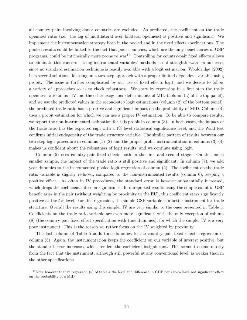
all country pairs involving donor countries are excluded. As predicted, the coefficient on the tradeopenness ratio (i.e. the log of multilateral over bilateral openness) is positive and significant. Weimplement the instrumentation strategy both in the pooled and in the fixed effects specifications. Thepooled results could be linked to the fact that poor countries, which are the only beneficiaries of GSPprograms, could be intrinsically more prone to war17. Controlling for country-pair fixed effects allowsto eliminate this concern. Using instrumental variables’ methods is not straightforward in our case,since no standard estimation technique is readily available with a logit estimation. Wooldridge (2002)lists several solutions, focusing on a two-step approach with a proper limited dependent variable usingprobit. The issue is further complicated by our use of fixed effects logit, and we decide to followa variety of approaches so as to check robustness. We start by regressing in a first step the tradeopenness ratio on our IV and the other exogenous determinants of MID (column (a) of the top panel),and we use the predicted values in the second-step logit estimations (column (2) of the bottom panel):the predicted trade ratio has a positive and significant impact on the probability of MID. Column (4)uses a probit estimation for which we can use a proper IV estimation. To be able to compare results,we report the non-instrumented estimation for this probit in column (3). In both cases, the impact ofthe trade ratio has the expected sign with a 1% level statistical significance level, and the Wald testconfirms initial endogeneity of the trade structure variable. The similar pattern of results between ourtwo-step logit procedure in columns (1)-(2) and the proper probit instrumentation in columns (3)-(4)makes us confident about the robustness of logit results, and we continue using logit.

Column (5) uses country-pair fixed effects both in the first and second stage. On this muchsmaller sample, the impact of the trade ratio is still positive and significant. In column (7), we addyear dummies to the instrumented pooled logit regression of column (2). The coefficient on the traderatio variable is slightly reduced, compared to the non-instrumented results (column 6), keeping apositive effect. As often in IV procedures, the standard error is however substantially increased,which drags the coefficient into non-significance. In unreported results using the simple count of GSPbeneficiaries in the pair (without weighting by proximity to the EU), this coefficient stays significantlypositive at the 5% level. For this regression, the simple GSP variable is a better instrument for tradestructure. Overall the results using this simpler IV are very similar to the ones presented in Table 5.Coefficients on the trade ratio variable are even more significant, with the only exception of column(8) (the country-pair fixed effect specification with time dummies), for which the simpler IV is a verypoor instrument. This is the reason we rather focus on the IV weighted by proximity.

The last column of Table 5 adds time dummies to the country pair fixed effects regression ofcolumn (5). Again, the instrumentation keeps the coefficient on our variable of interest positive, butthe standard error increases, which renders the coefficient insignificant. This seems to come mostlyfrom the fact that the instrument, although still powerful at any conventional level, is weaker than inthe other specifications.

17Note however that in regression (5) of table 4 the level and difference in GDP per capita have not significant effecton the probability of a MID.

26

Table 5: Impact of trade on MID - IV regressions

First Stage (dep. var: mul./bil. trade ratio)

Model: (a) (b) (c) (d) (e)

EU GSP Programme t-8 5.42a 5.42a 3.04a 2.49a 1.44a

(0.31) (0.31) (0.34) (0.31) (0.42)

Estimation method OLS OLS FE OLS OLS FE OLSF-test on IV 298 298 80 66 12R2 0.505 0.505 0.326 0.527 0.332

Second Stage (dep. var: MID)

Model: (1) (2) (3) (4) (5) (6) (7) (8)

ln mul./bil. trade ratio t-4 0.46b 0.16a 0.15b 0.42a

(0.20) (0.06) (0.07) (0.14)

ln dist. × ln mul./bil. trade ratio t-4 -0.06b -0.02b -0.06a

(0.03) (0.01) (0.02)number of peaceful years -0.03a -0.03a -0.01a -0.01a 0.02a -0.03a -0.03a 0.02a

(0.00) (0.00) (0.00) (0.00) (0.00) (0.00) (0.00) (0.01)war in t-1 3.00a 2.96a 1.73a 1.72a 2.24a 3.19a 3.22a 2.22a

(0.20) (0.20) (0.06) (0.07) (0.14) (0.13) (0.22) (0.22)ln distance -0.51a -0.41 -0.21a -0.28a -0.54a -0.32

(0.19) (0.30) (0.07) (0.08) (0.16) (0.32)

dummy for zero trade t-4 -0.34b -0.48 -0.14b -0.26c -3.52a -0.29c 0.33 -2.86(0.17) (0.34) (0.06) (0.15) (0.99) (0.15) (0.84) (2.54)

common language 0.14 0.13 0.05 0.05 0.21c 0.18(0.16) (0.16) (0.05) (0.05) (0.11) (0.16)

regional trade agreement -0.57a -0.53b -0.23b -0.23b -0.26 -0.55b -0.55b -0.31(0.22) (0.22) (0.11) (0.12) (0.41) (0.27) (0.23) (0.44)

nb of GATT/WTO members -0.30a -0.29a -0.14a -0.13a -0.09 -0.33a -0.36a -0.26(0.08) (0.08) (0.03) (0.03) (0.17) (0.08) (0.10) (0.31)

ever colonial link 0.64c 0.67c 0.31a 0.32a 0.65a 0.60(0.34) (0.34) (0.11) (0.11) (0.24) (0.38)

common colonizer -0.10 -0.09 -0.05 -0.05 -0.15 -0.16(0.19) (0.19) (0.06) (0.06) (0.14) (0.19)

contiguity 0.94a 1.00a 0.52a 0.53a 0.90a 0.83a

(0.19) (0.19) (0.06) (0.06) (0.14) (0.22)sum ln areas 0.16a 0.16a 0.05a 0.06a 0.17a 0.15a

(0.03) (0.04) (0.01) (0.01) (0.03) (0.04)sum of democracy indexes 0.09 0.08 0.02 0.02 0.22 0.00 -0.04 0.00

(0.14) (0.14) (0.05) (0.05) (0.19) (0.12) (0.17) (0.36)

UN vote correlation t-4 0.70b 0.58c 0.24b 0.19c 0.71b 0.13 0.07 0.74(0.32) (0.34) (0.10) (0.11) (0.31) (0.29) (0.35) (0.65)

pred. mul./bil. trade ratio t-4 0.67b 1.13b 0.37 0.84(0.31) (0.53) (0.40) (0.93)

ln dist. × pred. mul./bil. trade ratio t-4 -0.08c -0.01 0.00 -0.07c 0.01(0.04) (0.01) (0.06) (0.04) (0.06)

Estimation method logit logit probit 2S probit FE logit logit logit FE logitTime controls no no no no no yes yes yes

N 126544 126544 126544 126544 4971 126544 126544 4971Pseudo-R2 0.467 0.467 0.477 - 0.122 0.488 0.488 0.129

Note: Standard errors in parentheses with a, b and c respectively denoting significance at the 1%, 5% and 10%levels. In the first stage, coefficients of other exogenous variables (ie. the second stage controls) are notshown, standard errors are robust and clustered by country pair. In both stages, time controls consist ofyear dummies for columns (6) and (7), and decade dummies + a time trend for column (8).

27

3.5 Quantification

We now want to quantify the magnitude of the effect of trade on the probability of military conflictbetween two countries. First note that since our principal variables of interest are in logs, eachcoefficient is a very close approximation of the elasticity of war probability with respect to a changein the considered variable, when all variables are at their median value.18 A standard approach inour context is to imagine the following counterfactual experience. Take a pair of countries with amedian level for all variables, including bilateral and multilateral trade openness. Denote this countrypair’s initial probability of being in militarized dispute P . The interpretation of coefficients in termsof economic magnitude is here made difficult by the terms interacting openness with distance. Asemphasized by Ai and Norton (2003), the nonlinear nature of logit estimation makes it impossible tomake the usual linear adjustment to coefficients for different levels of distance.19 We therefore use theestimates on the sub-sample of proximate countries, given in column (2) of table 3. When estimated forpairs of countries separated by less than 1000 kilometers, the coefficients on bilateral and multilateralopenness are -0.11 and 0.37 and are significant both at the 5% level. A one standard deviation increasein both variables implies that median values increase by 123% and 218% respectively, which inducesa change in the probability of war of −14% and +81% respectively.

Historically, between 1960 and 2000, the bilateral openness variable has increased by 190% forthe median country pair separated by less than 1000kms. For the multilateral openness variable, theincrease is 179%. Using our point estimates, this means that the impact of bilateral trade has beento decrease the probability of bilateral war by around 22% for this median pair of countries. Theimpact of multilateral trade has been to increase this probability by around 66%. The net effect ofthis measure of globalization has therefore been to increase the probability of bilateral war by 44% inthe sample of proximate countries.

This seemingly pessimistic message illustrates the importance of the pattern of trade openness(bilateral vs multilateral): this pattern, which exhibits wide variations across country pairs, directlyinfluences the probability of conflicts. Let us consider the following illustrative example. France andGermany have in 2000 an average bilateral trade openness of 3.4% of GDP and an average multilateraltrade openness (excluding bilateral trade) of 22%. India and Pakistan, which experienced 36 conflictssince 1950, exhibit a different pattern: respectively 0.1% and 14%. We can use our econometric modelto address the following thought experiment: What would be the probability of conflict betweenIndia and Pakistan if those countries mimicked the Franco-German trade pattern? Using in-samplepredictions for 1995, our estimates show that the India-Pakistan probability of conflict drops from57% to 49%, mostly due to the increase in bilateral trade openness. The result is even more strikingif the trade structure was to mimic the Canada-US pattern as the estimated probability of war wouldthen drop to 39%. Interestingly, India and Pakistan are in the process of negotiating a large cut intheir tariffs within the South Asia Free Trade Area Agreement (SAFTA).

18The exact formula for this elasticity is β(1 − P ), where β is the obtained coefficient and P is the war probabilitygiven by the logit formula when all variables are at their median values (typically a small figure).

19we thank Harry Bowen for pointing out this issue.

28

4 Conclusion

Our paper is the first, to our knowledge, to highlight the opposite effects of bilateral and multilateraltrade on the probability of war and to base the empirical analysis on testable predictions generated bya theoretical model. Our results are somewhat ambivalent on the impact of trade and more generallyof globalization on the prevalence and the nature of war. We have shown that even in a model wheretrade increases welfare and war is Pareto dominated by peace, higher trade flows may not lead topeace. The intuition that trade promotes peace is only partially right: bilateral trade, because itincreases the opportunity cost of bilateral war indeed deters bilateral war. However, multilateral tradeopenness, because it reduces the opportunity cost of going to war with any given country, increases theprobability of war between any given pair of country. Trade globalization also affects the nature of war:multilateral trade openness increases the probability of local wars and deters global conflicts. This lastpoint is important: our paper should not be interpreted as suggesting that trade globalization leadsto war. Given that World Wars are certainly the most costly in terms of human welfare, this is not asmall achievement. We interpret more our paper as a word of caution and a possible explanation ofthe changing nature of wars.

Our model suggests a way through which multilateral trade openness and globalization couldbecome conducive to peace at the local level. Remember that the condition under which multilateraltrade increases the probability of war is that the increase in multilateral trade costs following a waris small. Our empirical analysis confirms this is the case. However, if countries in bilateral war wereto suffer large multilateral trade losses, for example through multilateral trade sanctions imposedby an international organization, then multilateral trade would become a deterrent to local wars.A second possible implication is that local trade integration should be encouraged by internationalorganizations.

Various extensions are possible on the impact of globalization on information flows and throughthis channel on the probability of war. A recent literature in trade (see Rauch 1999) has argued boththeoretically and empirically that trade in differentiated products (as opposed to homogenous productstraded anonymously) should generate more interactions between traders and therefore more informa-tion flows. Hence, we could more precisely test the impact of trade on war through the informationchannel by following Rauch distinction between differentiated and homogenous products.

Another possible extension is to focus on the impact of regional trade agreements on the probabilityof war and in particular to better understand which features of trade agreements are peace-promoting.This could provide an assessment of whether regional free trade, allowing for an increase in regionaltrade, is enough to augment peace prospects, or whether countries should be tied further by institu-tional and political ties.

29

References

[1] Ai C. and E. Norton, 2003, “Interaction terms in logit and probit models”, Economics Letters,80, 123-129.

[2] Alcala, F. and A. Ciccone, 2004, “Trade and Productivity,” Quarterly Journal of Economics119(2), 613–646.

[3] Alesina, A. and E. Spolaore, 1997, “On the Number and Size of Nations”, Quarterly Journal ofEconomics, 112(4), 1027-1056.

[4] Alesina, A. and E. Spolaore, 2003, The Size of Nations, MIT Press.

[5] Alesina, A. and E. Spolaore, 2005, “War, Peace and the Size of Nations”, Journal of PublicEconomics , 89(7), 1333-1354.

[6] Alesina, A. and E. Spolaore, 2006, “Conflict, defense Spending and the Number of Nations”,European Economic Review50(1), 91-120.

[7] Anderson, J. and E. van Wincoop, 2003, “Gravity with Gravitas: a Solution to the BorderPuzzle”, American Economic Review, 93, 170-92.

[8] Anderson, J. and E. van Wincoop, 2004, “Trade costs”. Journal of Economic Literature XLII,691-751.

[9] Anderton C. and J. R. Carter, 2001, “The Impact of War on Trade: An Interrupted Times-SeriesStudy”, Journal of Peace Research 38(4), 445457

[10] Baier, S. and J. Bergstrand, 2004, “Do Free Trade Agreements Actually Increase Members’International Trade”, mimeo University of Notre Dame.

[11] Baldwin R. and T.Murray, 1977, “MFN Tariff Reductions and Developing Country Trade BenefitsUnder the GSP”, Economic Journal, Vol. 87, 30-46.

[12] Barbieri, K, 1996, “Economic Interdependence: A Path to Peace or a Source of Interstate Con-flict?” Journal of Peace Research, 33(1), 29-49.

[13] Barbieri, K., 2002, The Liberal Illusion, Does Trade Promote Peace?, The University of MichiganPress.

[14] Barbieri, K. and G. Schneider, 1999, “Globalization and Peace: Assessing New Directions inthe Study of Trade and Conflict”, Journal of Peace Research, 36(4), Special Issue on Trade andConflict. 387-404.

[15] Bond B., 1986, War and Society in Europe, 1870-1970. New York: Oxford University Press.

[16] Chatterjee K. and W. Samuelson, 1983, “Bargaining under Incomplete Information”, OperationsResearch, 31, 835-851.

[17] Compte O. and P. Jehiel, 2005, “Inefficiencies in Bargaining: Departing from Akerlof andMyerson-Satterthwaite”, Mimeo, CERAS.

[18] Cremer J. and R. Mc Lean, 1988, “Full Extraction of the Surplus in Bayesian and DominantStrategy Auctions”, Econometrica 56, 1247-1257.

[19] Elliot Kimberly Ann , Jeffrey J. Schott , Gary Clyde Hufbauer and Barbara Oegg, 2005, EconomicSanctions Reconsidered, 3rd Edition , Institute for International Economics.

[20] Fearon J., 1995, “Rationalist Explanations for War”, International Organization, 49(3), 379-414.

[21] Feenstra, R., 2003, Advanced International Trade: Theory and Evidence, Princeton: PrincetonUniversity Press.

30

[22] Frankel, J., and D. Romer, 1999, “Does trade cause growth?” American Economic Review 89(3),379-399.

[23] Garfinkel, M., 1994, “Domestic politics and international conflict”, American Economic Review,84(5), 1294-1309.

[24] Garfinkel, Michelle R. and Skaperdas, Stergios, 2000, “Conflict Without Misperceptions or In-complete Information: How the Future Matters”, Journal of Conflict Resolution, 44(6), 793-807.

[25] Glick R. and A.Taylor, 2005, “Collateral Damage: Trade Disruption and the Economic Impactof War”, NBER Working Paper No. 11565.

[26] Grossman, H., 2003, “Choosing between peace and war”, NBER working paper 10180.

[27] Hess, G., 2004, “The Economic Welfare Cost of Conflict: an Empirical Assessment”, workingpaper Claremont Mc Kenna College.

[28] Hess, G. and A. Orphanides, 1995, “War politics: an economic, rational-voter framework”, Amer-ican Economic Review, 85(4), 828-846.

[29] Hess, G. and A. Orphanides, 2001, “War and democracy”, Journal of Political Economy, 109(4),776-810.

[30] Izquierdo A., Morisset J. and Olarreaga M., 2003, “Information Diffusion in International Mar-kets”, World Bank Working Paper No. 3032.

[31] Jones, D., S. Bremer and D. Singer, 1996, “Militarized Interstate Disputes, 1816-1992: Rationale,coding rules and empirical patterns”. Conflict Management and Peace Science, 15(2).

[32] Kapstein, E., 2003, “Two Dismal Sciences Are Better Than One Economics and the Study ofNational Security, A Review Essay”. International Security, Vol. 27, no. 3, pp. 158-187

[33] Keegan J., 1984, A History of Warfare. New York: Vintage.

[34] Kocs, S., 1995, “Territorial disputes and interstate war”, Journal of Politics 57(1), 159-175.

[35] Levy J., Walker Thomas and Edwards Martin, 2001, “Continuity and Change in the Evolutionof War”, in Zeev Maoz and Azar Gat (eds), War in a changing world. Ann Arbor: University ofMichigan Press; 15-48.

[36] Levy G. and R. Razin, 2004, “It takes two: An Explanation for the Democratic Peace”, Journalof the European Economic Association, 2(1), 1-29.

[37] Maddison, A., 2001, The World Economy: Historical Statistics, Paris: OECD.

[38] Mansfield, 1995, Power, Trade, and War, Princeton University Press.

[39] Morrow, J., R. Siverson and T. Tabares, 1998, “The Political Determinants of International Trade:The Major Powers, 1907-90”, American Political Science Review, Vol. 92, No. 3 September.

[40] Myerson, R. and M. Satterthwaite, 1983, “Efficient Mechanisms for Bilateral Trading”, Journalof Economic Theory, 29, 265-281.

[41] Oneal J. and B. Russett, 1999, “Assessing the Liberal Peace with Alternative Specifications:Trade Still Reduces Conflict”, Journal of Peace Research, 36(4), Special Issue on Trade andConflict. . 423-442.

[42] Polachek, S., 1980, “Conflict and Trade”, Journal of Conflict Resolution, 24(1), 57-78.

[43] Polachek, S., J. Robst and Y-C. Chang, 1999, “Liberalism and Interdependence: Extending theTrade-Conflict Model”, Journal of Peace Research, 36(4), Special Issue on Trade and Conflict:405-422.

31

[44] Powell, R., 1999, In the Shadow of Power: States and Strategies in International Politics , Prince-ton University Press.

[45] Rauch, James E., 1999, “Networks Versus Markets in International Trade,” Journal of Interna-tional Economics 48(1), 7-35.

[46] Romalis J., 2003, “Would Rich Country TRade Preferences Help Poor Countries Grow? EvidenceFrom the Generalized System of Preferences.”, Chicago GSB mimeo.

[47] Rose, A., 2003, “Which International Institutions Promote International Trade?”, forthcomingReview of International Economics.

[48] Rose, A., 2004, “Do We Really Know That the WTO Increases Trade?” American EconomicReview, 94(1), 98-114.

[49] Schneider, G and G. Schulze, 2005, “Trade and Armed Conflict: The Domestic Foundations ofCommercial Liberalism”. Mimeo, University of Konstanz.

[50] Skaperdas, S. and C. Syropoulos, 2001,“Guns, Butter, and Openness: On the Relationship Be-tween Security and Trade”, American Economic Review, Papers and Proceedings, 91(2), 353-357.

[51] Skaperdas, S. and C. Syropoulos, 2002, “Insecure Property and the Efficiency of Exchange,”Economic Journal, 112, 133-146.

[52] Staiger, D., and J. Stock, 1997, “Instrumental Variables Regression with Weak Instruments,”Econometrica, 557586.

[53] Subramanian, Arvind and Shang-Jin Wei, 2003, “The WTO Promotes Trade, Strongly, but Un-evenly”, NBER Working Paper 10,024.

[54] UNCTAD, 2003, “Trade Preferences for LDCs: an early assessment of benefits and possibleimprovements”.

[55] Van Creveld M., 1991, The Transformation of War. New York: The Free Press.

[56] Wooldridge, 2002, Econometric Analysis of Cross Section and Panel Data. Cambridge, MA: MITPress.

A Appendix 1: Solving for the second best protocol

This section derives the second best mechanism of our bargaining game under asymmetric information.To this purpose we rely on Myerson-Satherwaite (denoted M-S) and provide a two stage proof whichfollows Compte and Jehiel (2005). First, we study the equilibrium of a particular protocol, the so-calledNash bargaining protocol. We then show that this protocol implements the second best mechanism.

Remember that our setup differs from the M-S setup as 1) at any time, countries may quit ne-gotiations; 2) private information is partially correlated between countries: the outside options areuniformly distributed on the triangle Γ=(M,MA,MB) (see Figure 3).

Γ = (UWi , UW

j ) | (UWi , UW

j ) ≥(vi, vj

)and UW

i + UWj ≤ v

with vi ≡ (1 − V/2)UWi and vi ≡ (1 − V/2)UW

j and v = (1 + V )(UWi + UW

j ). From assumption (1),peace Pareto dominates war, meaning that v < SP ≡ UP

i +UPj . In the rest of the section, for the sake

of expositional clarity, we assume without loss of generality20 that V = 2 such that vi = vj = 0

20In figure 3, assuming V = 2 means that M corresponds to the origin (0, 0).

32

A.1 The Nash Bargaining protocol

The Nash bargaining protocol was first described in a slightly different setting by Chaterjee andSamuelson (1983). This is a two stage protocol.

• ”announcement stage”: In the first stage, both countries i and j announce an outside option(UW

i , UWj ) and a sharing rule is proposed.

If the announcements are compatible, that is, if the sum UWi + UW

j ≤ SP , an agreement isproposed along with transfers τi(UW

i , UWj ) and τj(UW

i , UWj ) chosen so that each party obtains

in addition to its announced outside option, half the surplus SP − (UWi + UW

j ) that is:

τi(UWi , UW

j ) = UWi +

SP − (UWi + UW

j )2

and τj(UWi , UW

j ) = UWj +

SP − (UWi + UW

j )2

In case the announcements are not compatible, UWi + UW

j > SP , the bargaining process stops,war is triggered and each party gets its (true) outside option (UW

i , UWj ).

• ”agreement stage”: In the second stage, parties sequentially report if they accept the deal21. Ifboth parties say ”yes”, the deal is implemented. Otherwise, negotiation stops, war is triggeredand each party gets its (true) outside option (UW

i , UWj ).

Clearly, in the second stage, it is a dominant strategy for each party k ∈ (i, j) with true outsideoption UW

k to say ”yes” (respectively ”no”) if τk ≥ UWk (respectively τk < UW

k ). From Compte andJehiel (2005), we are able to characterize the equilibrium of the outside option announcement game22:

Lemma 1: At equilibrium, a party k ∈ i, j with (true) type UWk announces UW

k = a(UWk ) where

a(UWk ) =

14Sp +

23UW

k

Consequently, there is an agreement and Peace is maintained when UWi + UW

j ≤ 34SP . War occurs

for UWi + UW

j > 34SP . On Figure 3, disagreement arises for every couple of outside options which are

located in the ABMBMA dashed area.Proof of lemma 1: The expected gain of player i with type UW

i when announcing UWi is

G(UWi , UW

i ) =∫

Sp−UWi

+a(UWj

)

2>UW

j

max(UWi ,

Sp − UWi − a(UW

j )2

)dUW

j

v−UWi

+UWi

∫Sp−UW

i+a(UW

j)

2<UW

j

dUWj

v−UWi

21This stage corresponds to our assumption of ”no commitment protocol”. In the M-S and C-S original approach, thisstage is not allowed: the parties agree ex-ante on the sharing rule; they cannot ex-post renegotiate.

22In the general case of V < 2, the formula becomes more complicated. Indeed a straightforward variable change showsthat in equilibrium, a party k ∈ i, j with (true) type UW

k announces UWk = a(UW

k ) where a(UWk ) = vk+ 1

4(Sp−vi−vj)+

23(UW

k −vk). Consequently, there is an agreement and Peace is maintained when (UWi + UW

j −vi−vj) ≤ 34(SP −vi−vj).

War occurs for (UWi + UW

j − vi − vj) > 34(SP − vi − vj).

33

We now check that it is optimal for party i to announce UWi = a(UW

i ). Given the form of a(.) it isreadily verified that whenever the announcements are compatible, i.e. a(UW

i )+a(UWj ) < Sp, we have:

a(UWk ) > UW

k for both k ∈ i, j. Hence the Nash bargaining share of each party k is above UWk . This

allows to simplify the expression of G(UWi , UW

i ) when UWi lies in the neighborhood of a(UW

i ) in:

G(UWi , UW

i ) =∫

a(UWj )<Sp−UW

i

Sp + UWi − a(UW

j )2

dUWj

v−UWi

+UWi

∫a(UW

j )>Sp−UWi

dUWj

v−UWi

Differentiating G(UWi , UW

i ) with respect to UWi yields:

∂G(UWi , UW

i )∂UW

i

=1

v−UWi

[b(Sp − UW

i )2

− (UWi − UW

i )b′(Sp − UWi )

]

where b(x) ≡ −38Sp + 3

2x is the inverse of function a(.). Straightforward computations show that

∂G(UWi , UW

i )∂UW

i

∣∣∣∣∣UW

i =a(UWi )

= 0

A.2 Second Best

We now show that the Nash bargaining protocol described in the previous section implements thesecond best. From M-S (1983), we know that when outside options are uniformly distributed on thesquare (UW

i , UWj ) ∈ [0, Sp]× [0, Sp] the second best (requiring interim participation constraint but not

an ex-post one) is implemented by the Nash bargaining protocol and leads to an agreement wheneverUW

i + UWj ≤ 3

4SP . But this is also the domain of agreement induced by the Nash Bargaining protocolin our model where outside options are uniformly distributed on the triangle Γ which can be viewed asa restriction of the uniform distribution to a subset of [0, Sp]× [0, Sp]. This implies that the allocationresulting from the Nash Bargaining protocol induces the second-best in our particular setup.

Indeed by contradiction, assume that in our setup where outside options are uniformly distributedon the triangle Γ, there is a mechanism Ω that generates a strictly higher expected welfare than theNash Bargaining Protocol. It would then be possible to improve upon the second best of the M-Ssetup, which we call the MS mechanism. To this purpose, note that any ”no commitment” truthfuldirect mechanism (ie. satisfying the ex-post participation constraints) is a truthful mechanism inthe M-S setup (ie. satisfying the interim participation constraint). Hence in the M-S setup, we canbuild a mechanism Ω′ stipulating: for (UW

i , UWj ) ∈ Γ, we have Ω′(UW

i , UWj ) = Ω(UW

i , UWj ); and

for (UWi , UW

j ) ∈ [0, Sp]2 − Γ, we have Ω′(UWi , UW

j ) = MS(UWi , UW

j ). From the previous remark,such a mechanism Ω′ is a truthful direct mechanism. Moreover as Ω generates a strictly higherexpected welfare than the Nash Bargaining Protocol on Γ, we have that Ω′ generates a strictly higherexpected welfare than the Nash bargaining protocol on the whole domain [0, Sp] × [0, Sp]. But thisis in contradiction with the fact that the Nash bargaining protocol is the second best for (UW

i , UWj )

uniformly distributed on [0, Sp]× [0, Sp].

34

B Appendix 2: equilibrium value of the probability of war.

Country i’s welfare under peace is UPi = U(xi) where xi ≡ (Li, Lj , Tij , Tih); under war, country i’s wel-

fare is stochastic (see equation (2)) but equal on average to an equilibrium value UWi = U [xi(1−∆)]

with: ∆ ≡ (λ, λ,−τbil,−τmulti). The probability of escalation to war between country i and countryj, given by (3), is then:

Pr(escalationij) = 1− 14V 2

[U(xi)− U(xi(1−∆)) + U(xj)− U(xj(1−∆))]2

U(xi(1−∆))U(xj(1−∆))

To obtain closed-form solutions we assume that the two countries are identical (however, they maybe different from the other countries in the world): xi = xj . We restrict our attention to first ordereffects and use a Taylor expansion around an equilibrium where countries are identical, such that:

Pr(escalationij) ' 1− 1V 2

[∆∇U(xi)U(xi)

]2

which can be rewritten, using (7) as equation (8) in the text with

W1 ≡ 1 + 1σ−1

LiRP

h=1LhT 1−σ

ih

+LjT 1−σ

ij

RP

h=1LhT 1−σ

ih

= 1 + 1σ−1

(miiEi

+ mij

Ei

)> 0

W2 ≡LjT 1−σ

ij

RP

h=1LhT 1−σ

ih

= mij

Ei> 0;W3 ≡

R∑h 6=j,i

LhT 1−σih

RP

h=1LhT 1−σ

ih

=R∑

h 6=j,i

mihEi

> 0

Using the national accounting identity:miiEi

+ mij

Ei+

R∑h 6=j,i

mihEi

= 1, we obtain equation (9) in the text.

Differentiating (8) with respect to Tij yields results mentioned in the text:

d Pr(1− escalationij)d (−Tij)

= 2Pr(1−escalationij)1/2 σ − 1V

mij

EiTij

τbil

(1− mij

Ei

)+(

λ

σ − 1− τmulti

) R∑h 6=j,i

mih

Ei

Differentiating (8) with respect to Tih yields:

d Pr(1− escalationij)d (−Tih)

= −2 Pr(1−escalih)1/2 σ − 1V

mih

EiTih

τbilmij

Ei+(

λ

σ − 1− τmulti

)1−R∑

h 6=j,i

mih

Ei

Using these two equations in the case of identical countries, we obtain the effect of globalization:

d Pr(1− escalationij)d (−T )

= −2 Pr(1− escalationij)1/2 σ − 1V

mihmii

E2i T

(R− 2)(

λ

σ − 1− τmulti −

τbil

R− 2

)which proves Result 1.

35

C Appendix 3: Examples of conflicts.

Table 6 provides examples of representative conflicts that are classified as MIDs in our sample. Foreach hostility level, two cases with narratives from the correlates of war project are presented.

Table 6: Narratives of representative MIDs

Countries involved Hostility level Short narrative

Guatemala/Belize 3 1993: Guatemala had long claimed the British colonyof British Honduras (Belize) to be Guatemalan territory.Guatemalan residents along the border with Belize claimedthat Belizean soldiers made an incursion to Guatemala anddestroyed corn and rice crops. Belize claimed that the sol-diers were operating on Belizean soil. As a response, theGuatemalan government dispatched 60 soldiers to the dis-puted border. No further incidents occurred in the imme-diate aftermath of the incursion.

Togo/Ghana 3 1994: Togo claims an incursion of 100 fighters (irregulars)from Ghana and accuses Ghana of supporting rebels. Togocloses its border with Ghana based on this claim. Ghana de-nies any involvement and accuses Togo of aggression. ThisMID is the border closing by Togo.

Cameroun/Nigera 4 1995: Camerounian troops attacked a Nigerian post, cap-tured it and lost it later in a Nigerian counteroffensive.

USA/Iraq 4 The FBI determined that the Iraqi government undertook aplot to assassinate former President Bush when he visitedKuwait in mid-April, 1993. The Clinton administrationretaliated by launching a cruise missile strike against anIraqi intelligence facility in downtown Baghdad.

Ethiopia/Eritrea 5 In May 1998, border skirmishes between Ethiopia and Er-itrea spun into the world’s largest conventional war at thetime. The war displaced hundreds of thousands of resi-dents and claimed several thousands causalities. In June2000, Ethiopia and Eritrea signed a cease-fire, December12, 2000 they signed a permanent peace treaty.

Jordan, Egypt,Syria, Iraq/Israel

5 1966-67: Six Day War Jordan, Egypt, Syria and Iraqagainst Israel

36