1

Maker-Taker Pricing Effects on Market Quotations

Larry Harris*

USC Marshall School of Business

November 14, 2013

Draft 0.91

(Complete draft but comparative analyses of high price stocks and earlier sample periods

are yet to be done.)

Abstract

The exchange maker-taker pricing scheme affects incentives to take or make markets resulting in narrower bid-ask spreads. This study traces the effect of maker-taker pricing on stock quotations. The analyses consider distributions of quotation sizes, values implied from these sizes, and changes in these sizes and values. The results help inform the current debate on whether tick sizes should be made smaller for actively traded low price stocks. They also shed light on various problems associated with maker-taker pricing and its cousin taker-maker pricing, which allows traders to engage in sub-penny quotation behavior that legally violates the spirit of Regulation NMS.

Keywords: Exchange fees, maker-taker, taker-maker, access fees, liquidity rebates, quotation sizes, microprice, tick size, minimum price variation, bid-ask spread

*Contact the author at lharris@USC.edu; Bridge Hall 308, USC Marshall School of Business, Los Angeles, CA 90089-0804; or +1 (213) 740-6496. The author gratefully acknowledges discussions with Robert Battalio, Naftali Harris, Joel Hasbrouck, Jonathan Karpoff, and Ingrid Warner; and research assistance provided by Georgios Magkotsios.

2

1 Introduction Exchanges changed how they price their services over the last 15 years. Traditionally, they charged a small fee to the buyer, the seller, or both. Now most exchanges charge a relatively high fee to the trade initiator (the taker) and rebate most of it to the liquidity supplier (the maker). Liquidity suppliers are buyers or sellers whose standing limit orders or quotes provide options to trade. They make markets. Trade initiators are sellers or buyers who take these options to trade by submitting marketable orders.

The fees charged to the takers are called access fees. For equity trades, the access fees typically are 0.30¢/share (3 mil or “30¢ a hundred”). The liquidity rebates received by the makers are typically 0.25¢/share. The difference between the access fee and the liquidity rebate is the net revenue that exchanges receive for providing exchange services—collecting orders, displaying orders when permitted, and arranging trades when possible. This net difference is approximately the same amount that traditional fee exchanges would collect in total from buyers and/or sellers when arranging trades.

Although maker-taker fees are a very small fraction of trade prices, the total money transferred from takers to makers in U.S. equity markets is quite significant due to their high trading volumes. Cardella, Hao and Kalcheva (2013) calculate that this flow amounts to approximately $2B/year.1

Economic theory suggests that the introduction of maker-taker pricing should have narrowed average bid-ask spreads by approximately twice the access fee or the liquidity rebate rate. All other things equal, such a narrowing would keep constant the net bid-ask spread—the quoted spread adjusted for fees paid by takers or rebates received by makers) that takers pay and makers receive. The theory of equilibrium spreads, which Cohen, Maier, Schwartz, and Whitcomb (1981) (“CMSW”) first formalized, suggests that traders choose to be takers or makers based on the net spreads that they pay or receive. Since the maker-taker pricing scheme essentially simply involves a transfer from the takers to the makers, in competitive equilibrium, spreads should narrow to offset the transfer.

In practice, two issues make it near impossible to observe the expected decrease in spreads. Most importantly, many other factors that affect bid-ask spreads have changed over the last 15 years. The most important of these factors has been the introduction of electronic exchange trading systems and the associated growth of electronic dealers. These innovations greatly reduced the costs of trading and therefore undoubtedly substantially reduced bid-ask spreads. The observed reduction in bid-ask spreads over the last 15 years documented by numerous authors2 cannot be entirely attributed to the introduction of maker-taker pricing, which occurred at different times for various exchanges.

Second, spreads cannot decrease for stocks that already trade at one-tick spreads. Instead, when liquidity rebates make offering liquidity more attractive, quotation sizes increase as makers compete to trade at attractive prices. Note however, that an empirical study of

1 See Table II of their study.

2 See for example, Angel, Harris, and Spatt (2010 or 2013).

3

quotation sizes also cannot identify the effect of maker-taker pricing for the same reasons that a study of bid-asks spreads cannot do so: Too many other factors that determine quotation sizes also have changed.

This study identifies secondary empirical effects of maker-taker pricing by examining characteristics of market data that are more uniquely related to maker-taker pricing than are average bid-asks spreads and quotation sizes. In particular, the results presented here show that quoted prices are more informative when adjusted for access fees and liquidity rebates. These results are a direct consequence of the fact that most sophisticated traders are concerned about net prices and not quoted prices. This evidence thus strongly suggests that maker-taker pricing indeed has affected average bid-ask spreads and average quotation sizes for stocks often trading at one-tick spreads.

These results are important to practitioners, regulators, and academics. Practitioners are interested because access fees and liquidity rebates are often large components of overall transaction costs, especially for small trades in low price stocks. For example, when the quoted bid-ask spread is 1¢, the average cost of taking the market is one-half the spread plus the 0.3¢ access fee.3 The net cost, 0.6¢/share, is 60% larger than the cost based only on the quoted spread. Practitioners, whether on the buy-side or sell-side, will make better trading decisions by focusing on net prices rather than quoted prices.

Several concerns motivate regulator interest in maker-taker pricing:

1. As discussed in detail in the next section, maker-taker pricing creates an agency problem between brokers and their clients when the clients do not receive the liquidity rebates or when business models prevent brokers from passing on the access fees.

2. Maker-taker pricing creates a transparency problem since quoted spreads are different from the more economically meaningful net spreads and since most retail traders are unaware of the difference.

3. Maker-taker pricing and its recent variant, taker-maker pricing (discussed in the conclusion), represent a means by which exchanges can permit net quotes on sub-penny increments. These pricing models thus represent loopholes through which exchanges and their more sophisticated clients can subvert the prohibition on sub-penny quotation pricing in Regulation NMS. This loophole allows sophisticated electronic traders to front-run buy-side traders.

4. Maker-taker pricing increases incentives to route market orders for execution in venues that do not charge access fees. These venues include dealers who internalize their client order flows, dealers who pay brokers to preference their customers’ orders them, and various dark pools that match buyers and sellers.

3 To easily see that the average cost of taking is half the bid/ask spread, consider the total loss associated with the

simultaneous submission of a small market buy order and an equal-sized market sell order. The two trades will accomplish nothing except for the completion of a round-trip trade that loses the bid/ask spread for each share traded. The cost per share of one trade thus is half of the bid/ask spread.

4

5. Finally, maker-taker pricing makes markets unnecessarily complex at the cost of creating agency problems and without the benefit of adding any positive value. Financial risk managers trained in systems engineering recognize that complexity is an important cause of systemic risk.4 The additional complexity associated with maker-taker pricing works against efforts to reduce systemic risk.

Maker-taker pricing interests academics for the opportunity to empirically explore implications of the equilibrium spread theory (as done in this study) and to examine associated agency problems.

The regulatory problems associated with the maker-taker pricing scheme also have generated substantial attention from politicians. For example, Senator Charles Schumer, among others, has called upon the SEC to require that liquidity rebates be passed through to clients.5

1.1 Non-price Competition

The results in this study are also interesting because they show how traders compete to offer liquidity when the minimum price variation (“tick”) sets a binding lower bound on bid-ask spreads. This topic interests regulators, practitioners and academics because a large tick prevents price competition among traders. Instead traders must queue to get their orders executed. Many people now think that tick sizes are too small for some low priced actively traded securities, and the SEC is considering a pilot study which would permit a smaller tick for the most actively traded low price stocks.

This paper examines how these securities trade. The results strongly support the view that makers compete to offer size when the minimum price variation prevents them from offering better prices. This competition causes quotation sizes to reflect trader information about values. Since maker-taker pricing affects quotation decisions, the information in the quoted sizes is best extracted by adjusting for the maker-taker fees and rebates.

The two topics—the impact of maker-taker pricing and the effects of a large minimum price variation—are closely linked to each other. By narrowing net spreads, maker-taker pricing partially mitigates the importance of the minimum price variation. And a large minimum price variation minimizes the economic importance of maker-taker pricing.

The organization of this article is as follows: Section 2 presents a quick description of the growth of maker-taker price and its implications for trader behavior. The next section outlines the empirical study. Section 4 describes the data while Section 5 provides the main empirical results. The article concludes in Section 6 with a discussion of implications for market structure.

4 See Bookstabbler (2007).

5 See Schumer (2012).

5

2 Maker-Taker Pricing

2.1 History

Soon after ECNs started business in the US, they adopted maker-taker pricing schemes to attract more liquidity to their systems.6,7 The first system to introduce this scheme was Island ECN in 1997.

The liquidity rebates encouraged brokers to post customer limit orders in their systems, which generated revenues for these brokers when these customer orders executed. The rebates also encouraged proprietary traders to make markets in their trading systems. Since takers paid the high access fee when trading with these orders, brokers and proprietary traders typically routed their taking orders first to traditional-fee exchanges (and off exchange-dealers) when the same prices were available at these other trading venues. The standing orders at maker-taker exchanges thus usually were the last orders to trade at their prices. Although this consequence was disadvantageous to the customers, in the absence of regulatory criticism of this obvious agency problem, the brokers continued to route customer orders to the ECNs to obtain the liquidity rebates. To remain competitive, all US equity exchanges ultimately adopted the maker-taker pricing model.

The competition for order flow among ECNs using the maker-taker pricing model encouraged the ECNs to play a game of leap frog in which they took turns increasing their liquidity rebates (and associated access fees) in attempts to attract more order flow. This competition reached its apex when the ATTAIN ECN charged non-subscribers 1.5¢/share access fees in 1998. The SEC Division of Market Regulation (since renamed Trading and Markets) put a stop to this game with an interpretive letter that effectively limited access fees to 0.3¢/share. This limit later was formally incorporated into Regulation NMS in 2005. Most access fees are now at or just under 0.3¢/share.8

The typical difference between access fees and liquidity rebates used to be 0.1¢/share, which was approximately the level of the typical traditional exchange transaction fee. Competition among electronic exchanges over the last few years has pushed this difference down to approximately 0.05¢/share.

The US options markets now are almost all maker-taker markets with the exception of the CBOE, which remains a traditional fee market. (The CBOE also runs the fully electronic maker-taker C2 Options Exchange as a separate exchange.) However, order routing in traditional fee options markets is strongly influenced by payments for order flow made by designated dealers, which are essentially negative access fees.

6 ECNs (Electronic Communications Networks) are a class of non-exchange electronic trading systems run by

broker-dealers that the SEC permitted with the adoption of Regulation ATS. Many of the surviving ECNs have since become exchanges. Examples of successful early ECNs include Island ECN (later bought by Instinet, which was then bought by NASDAQ), Archipelago ECN (later bought by the Pacific Stock Exchange, which was then bought by the NYSE), and BATS ECN, which became the BATS Exchange in 2008. 7 Island ECN introduced the first maker-taker fee schedule in 1997.

8 See Cardella, Hao and Kalcheva (2013) Table I for a characterization of the average fee structure at US exchanges.

Foucault, Thierry, Ohad Kadan, and Eugene Kandel (2013) Table I also provides a summary of make and take fees.

6

2.2 Implications

Holding constant the quoted bid and ask prices, the 0.3¢/share access fee effectively increases net bid-ask spreads paid by makers by 0.6¢/share over the quoted market spreads. Buyers who initiate trades pay the quoted ask price plus the 0.3¢ access fee while taking sellers receive the quoted bid price less the 0.3¢ access fee. The net spread received by makers likewise increases by approximately 0.5¢/share.

These changes in net spreads affect the incentives to take or make markets. In particular, holding constant the quoted spread, the access fees render taking liquidity less attractive, and the liquidity rebates render making markets more attractive. Following the adoption of maker-taker pricing, quoted bid-ask spreads thus had to decrease to restore the equilibrium between taking and making first formally described in CMSW.

The CMSW equilibrium spread model describes how bid-ask spreads regulate whether traders take or make markets. When spreads are too wide, making markets is more attractive than taking markets and overall volumes drop as most traders want to make markets and few are willing to take markets. As traders switch from taking to making, they quote more aggressively as they compete to trade and they thereby decrease spreads and restore equilibrium. Likewise, when spreads are too narrow, taking markets is more attractive than making markets and overall volumes drop as most traders want to take markets but few are willing to make markets. The competition to take markets widens spreads and restores equilibrium. The equilibrium spread occurs at quoted spreads that equate the total volume that trade initiators want to trade to the total volume the makers want to trade.

A trivial extension of the CMSW model predicts that, holding all other things constant, average quoted spreads should have decreased by approximately 0.6¢/share following the widespread adoption of maker-taker pricing. The uncertainty in the prediction is due to uncertainty about the burden of the net exchange fee of 0.5¢. If the entire burden falls on the takers, an access fee of 0.3¢/share would narrow by spreads by 0.6¢. The elimination of a 0.05¢ traditional fee would further reduce spreads by 0.05¢, for a net decrease of 0.65¢. In contrast, if the entire burden falls on the makers, a liquidity rebate of 0.25¢/share would narrow by spreads by 0.5¢. The elimination of a 0.05¢ traditional fee would further reduce spreads by 0.05¢, for a net decrease of 0.55¢.

In practice, as noted in the introduction, many concurrent changes in the markets make identifying such a decrease empirically very challenging. Moreover, the one-tick minimum price variation prevents the quotation of tighter bid-ask spreads for those stocks that commonly are quoted with one-tick spreads. For these stocks, maker-taker pricing presumably increases displayed sizes as traders compete to obtain the liquidity rebates.

2.3 Related Literature

Two event studies consider new adoptions of maker-taker pricing schemes to identify the effects of the change in the exchange pricing scheme. These studies are one-shot event studies for which controls for other effects on spreads may be difficult. Malinova and Park (2011) analyzes the 2005 introduction of maker-taker pricing at the Toronto Stock Exchange. They find that spreads narrowed and depths increased. Lutat (2010) analyzes the 2008 introduction of

7

maker-taker fees on the SWX Europe Exchange and shows that spreads were unchanged but quotation sizes widened.

Two studies examine the effects of changes in maker-taker fees in U.S. equity markets. Cardella, Hao and Kalcheva (2013) shows that exchange volumes depend on relative fees, but cannot identify an effect on spreads in a study of data from 2008 to 2010. Skjeltorp, Sojli and Tham (2013) uses changes in exchange volumes following changes in maker-taker fees to identify the value of the order flow externality.

Three theoretical studies examine the impact of maker-taker pricing on exchange revenues and overall welfare. Foucault, Kadan, and Kandel (2013) studies the determinants of trading rates and find that asymmetric fees can maximize the trade rate when the tick size is a binding constraint on bid-ask spreads. Otherwise, their model broadly supports the CMSW equilibrium results. Colliard and Foucault (2012) examines a model that considers the effect of net trading fees—the difference between the access fee and the liquidity rebate—on the competition among markets. Their results are generally consistent with CMSW. Brolley and Malinova (2012) examines the effect of maker-taker fees on markets and show that distortions result when the maker-taker fees and rebates are not passed through to brokerage customers. The customers take liquidity more often than they otherwise would.

Battalio, Shkilko, and Van Ness (2011) compares maker-taker pricing schemes used by some U.S. options markets to attract liquidity-supplying orders with payment for order flow schemes used by other options markets to attract market orders. Although both types of markets are order-driven, limit order traders provide most of the liquidity in the former markets whereas dealers provide most of the liquidity in the later markets. The differences in market structure make the results largely irrelevant to the issues explored in this study.

3 Empirical Predictions Simple economic principles suggest that rational traders will consider fees and rebates when making quotation and trading decisions. As discussed above, these considerations should lead to tighter spreads and greater quoted sizes for stocks that often trade with one-tick spreads. Although these primary effects cannot be easily identified, other effects of the fees and rebates can be.

In particular, maker-taker fees and rebates should affect the prices and quantities that traders quote conditional on their estimates of value. Accordingly, estimates of value based on quoted prices and sizes should be more informative if they account for the maker-taker fees and rebates than if they do not.

The empirical strategy that I use to identify the effects of maker-taker price examines estimates of stock values obtained from quoted prices and sizes. I show that these estimates are more informative when the estimates account for maker-taker fees and rebates. I also examine implications of maker-taker pricing for the distributions of these value estimates and confirm that they are present in the data.

The measures of value informativeness are described below. They are based on simple estimates of value obtained from quoted prices and sizes.

8

3.1 Value Estimates

Suppose that the market quote for a stock is $5.01 bid for 1,000 shares, with 1,000 shares offered at $5.02. If forced to provide a single estimate of the unobserved full-information value of the stock (the “true value”) given this information only, most people will estimate true value at the quotation midpoint, 1.5 ($5.015).

To simplify the discussion, I will refer to quotes as practitioners do: They would say that the market is “1 bid for 10, 10 offered at 2” where the 1 and 2 are understood to be cents with the $5 whole number part of the price assumed, and the 10 refers to 10 lots of 100 shares each. The further clarify the presentation, I will present market quotes within curly brackets as follows: {1 bid for 10, 10 offered at 2} or sometimes simply as {1, 2}.

Now suppose that the market is {1 bid for 28, 12 offered at 2}. Based only on this information, sophisticated market observers will note that the relative paucity of selling interest at the ask (2¢) in comparison to the much larger buying interest at the bid (1¢) suggests that overall, market participants think that the opportunity to buy at 1¢ is more attractive than the opportunity to sell at 2¢. Such a conclusion is consistent with the inference that true value is closer to the ask than to the bid.

If we assume that 1) demand and supply schedules are linear in the difference between potential trade prices and unobserved true values, 2) the absolute values of the slopes of these schedules are equal, and 3) supply and demand are both equal to zero when price is equal to unobserved true value, we can estimate the unobserved true value from the quoted prices and sizes. In particular, we simply express the slopes of both schedules as a function of the market quote and the true value, , and solve for the true value:

(1)

The resulting estimate is the size-weighted average of the bid and ask prices where the bid is weighted by the ask size and the ask is weighted by the bid size:

(2)

It can also be expressed as

(3)

where

is the ratio of the two quotation sizes. The estimate thus depends only on the ratio

of the two sizes and not their absolute levels. Is the spread between the bid and ask is , the estimate can be expressed as

(

) (4)

where

is the quote midpoint.

9

Practitioners sometimes call this estimate of true value the microprice.9 It is represented

graphically in Figure 1 by Point M where angles 1 and 2 are equal. In the above example,

the value estimate is

.

The following three observations provide theoretical foundations for this value estimate:

1. The linear supply and demand schedules that motivate the derivation of this estimate are easily derived from the maximization of an exponential utility function, which generally can serve as a local approximation to any utility function.

2. Alternatively, linear demand and supply functions with equal absolute slopes and that intersect where size is equal to zero can be taken as local approximations to any demand and supply functions that 1) depend only on common value estimates and 2) are not subject to profitable bluffing strategies as described in Kyle (1985). The first condition ensures that the demand and supply are zero at the common best estimate of true value while the second condition ensures that the absolute values of the two slopes are equal.

3. Finally, expressions involving size-weighted averages of prices also appear as the market clearing price in simple continuous linear demand models in which traders do not have common value estimates such as in the models introduced in Grossman and Stiglitz (1980).

3.2 The Adjusted Value Estimate This value estimate does not take into account maker-taker access fees and rebates. Accordingly, we will refer to it as the unadjusted value estimate. As discussed above, the net bid price is approximately 0.3¢ smaller than the quoted bid price and the net ask price is approximately 0.3¢ larger than the quoted ask price. On the assumption that rational traders take these fees and rebates into account when pricing and sizing their orders, the best estimate of true value given the assumptions described above is the solution for to the following formula, where represents the access fee, rebate, or some midpoint between the two:

( ) (5)

The solution is

( )

( ) (6)

which also can be expressed as

( )

( ) (7)

or

9 In the academic literature, the microprice has been used by Gatheral and Oomen (2010), Avellaneda, Reed, and

Stoikov (2011), Burlakov, Yuri, Michael Kamal, and Michele Salvadore (2012) and others.

10

(

) (

) (8)

The adjusted value estimate expressed in terms of the unadjusted value estimates is

(9)

The adjusted value estimate is equal to the unadjusted estimate plus an adjustment that is equal to the fee times half the percentage difference between the bid and ask sizes calculated relative to their average value. This result shows that the adjustment is small when the bid and ask sizes are close to each other so that is near one. However, the adjustment can grow to as one or the other size grows large relative to the other.

Figure 2 illustrates the computation of the adjusted true value estimate when the maker-taker fees paid and rebated are taken into account. In geometric terms, the adjustment moves the estimate away from the unadjusted estimate in the direction of the smaller quote size because the adjustments to the quoted bid and ask prices to obtain the net bid and ask prices are of equal size. The value estimate moves toward the side with the smaller size because the unadjusted estimate is closer to that side.

3.3 Implications for Informative Prices If traders indeed consider maker-taker pricing when making trading decisions, the values estimated by the adjusted value estimator should be closer to true values than the values estimated by the unadjusted value estimator. Furthermore, both estimators should be closer to true value than the midpoint of the spread.

These predictions cannot be tested directly because true values are not known. But they can be tested indirectly by examining properties that we expect good estimates of true value to have. In particular, analyses of cross-sectional correlations, time-series variances, and time-series serial covariances can reveal which estimators are least noisy.

These analyses are all based on statistics computed from changes in estimated values. These changes will have less noise when estimated from good estimates of true value then from poor estimates.

Stock true-value returns are undoubtedly correlated in cross-section because stock valuations depend on common factors. Cross-sectional correlations computed from good estimates of true value thus should be higher than those computed from poor estimates.

In principle, tests of the quality of a value estimate could be based on serial correlation of its estimated value changes. On the assumption that true value changes are serially uncorrelated, estimators that produce serial correlations that are close to zero may be better than those that produce serial correlations further from zero. The problem with this test is that it implicitly assumes that true value changes are serially uncorrelated at the high frequencies observed in microstructure data. While in perfect markets, true value changes should be serially uncorrelated, most people believe that market microstructure frictions induce positive or negative serial correlations into high frequency data, depending on the nature of the friction.

11

Accordingly, inferences in this study based on serial correlations will be problematic. A similar criticism applies to inferences based on the time-series variances.

3.4 A Useful Surprise

Close consideration of the adjusted value estimate reveals an unexpected characteristic: The adjusted value estimate can be outside the quoted market. The adjusted value estimate will be greater than the ask when the bid size is a large multiple of the ask size, and it will be less than the bid when the ask size is a large multiple of the bid size.

This observation in turn reveals a somewhat surprising and important characteristic of the adjusted value estimate: Within certain ranges of value near the discrete price ticks, the same value estimate may be computed for different markets quoted on either side of a price tick. For example (illustrated in Figure 3), two market quotes can imply the adjusted value estimate of 2.14: {1 bid for 36, 4 offered at 2} and also {2 bid for 11, 29 offered at 3}. The common 2.14 value estimate is outside of the {1, 2} market and inside the {2, 3} market.

Note that although the bid and ask sizes are asymmetric in both markets, the asymmetry is greater in the market for which the estimate is outside of the spread, in this case, the {1, 2} market where the ratio of bid size to ask size is 36:4 or 9:1. In the {2, 3} market, the ratio of ask size to bid size is 29:11, or approximately 2.6:1.

3.5 Implications for Distributions

This last characteristic of the impact of maker-taker fees and rebates on prices and quantities (overlapping value ranges) is unique to the maker-taker pricing scheme. It thus permits empirical identification of the impacts of these fees on the markets. In particular, this feature of the valuation estimates has strong and unique implications for the unconditional distribution of the sub-penny part of valuation estimates and for the conditional distribution of these sub-penny parts given lagged valuation estimates.

3.5.1 Univariate Implications

For example, the sub-penny distribution of true values between discrete price ticks presumably is approximately uniform because the ticks are very close together:

( ) [ ] (10)

Accordingly, the expected distribution of the sub-penny component of fee-adjusted value estimates likewise should be uniform.

Note however, that if sub-penny values are uniformly distributed between the discrete ticks, the distribution of the sub-penny component of the unadjusted value estimates will not be uniform. Instead, the density in the tails (values close to the discrete ticks) will be lower than the density in the middle.

This result is easiest to understand in markets with one-tick spreads. In such markets, a low or high sub-penny adjusted value estimate can arise in two different adjacent markets, for example, {1,2} and {2,3}, whereas a middling value only can arise in a single market. Adjusted

12

value estimates only can arise in a single market when true value is within the range defined by

(11)

or equivalently,

(12)

since the lowest true value that can be expressed in the one tick higher market is and the highest true value that can be expressed in the one tick lower market is . Within these bounds for , the unadjusted value estimates range over a narrower range than do the adjusted value estimates because they are always closer to the midpoint then are their associated true values. Since the integrated densities for the two variables in their respective ranges must be the same because they both map one-to-

one to in this region, the average density in this middle range of must be greater than the

assumed uniform density for within this region. Thus ( ) cannot be uniformly

distributed over its entire [0¢, 1¢) range. It will have greater density near the quote midpoint than near its tails.

If no other processes affect the distribution of the unadjusted estimates, they should be uniformly distributed in this middle range because they are simply a linear contraction towards the quote midpoint of the true values, which we presume are uniformly distributed between price ticks. In practice, many other processes also may affect the distribution of unadjusted quotes so a uniform distribution in this range may not be observed.

The bounds in equation (11) can be expressed in terms of by deriving an expression for as a function of . This in turn requires an expression for the quotation size ratio, , as a function of . To derive the second expression, for solve equation (8) under

the assumption that to obtain the implied by a true value for a given and . It is

( )

(13)

Substituting this expression into equation (4) produces an expression for the unadjusted

estimate as a function of the true value . It is

(

) (14)

Note that

( ) (

) (15)

is less than when and greater otherwise so that is always closer to than is

Inverting equation (14) provides an expression for in terms of

13

( )( )

(16)

Substituting this expression into equation (4) gives the desired bounds for within which the associated true value must be between the current bid and ask prices:

(

)

(

) (17)

For (the average of 0.25¢ and 0.3¢) and , this range is approximately

[ ]. Although this range is only 29.0% of the total 1¢ range of ( ), it has

( ) of the integrated density, or

approximately 45.0% for .

The shape of the distribution in the tails is less obvious. It depends on the processes that cause quoted prices to rise or fall because they determine how often true value is outside of the current market.

Before considering such processes, consider how the tail values of the sub-penny distribution of

( ) arise in one-tick markets. For in the range [ ] any value that can

be implied from a quote in the market can also be implied from a quote in the

market . ( ) will be in the right tail of the sub-penny distribution in

the former case and in the left tail in the latter case. Note also that for in the range [ ] any value that can be implied from a quote in the market can

also be implied from a quote in the market . ( ) will be in the left

tail of the sub-penny distribution in the former case and in the right tail in the latter case. Thus

( ) values in the right tail can arise when the market is and is in [ ] or when the market is and is in [ ].

Likewise, ( ) values in the left tail can arise when the market is { and is in [ ] or when the market is and is in [ ].

Processes that cause quotes to shift up or down presumably depend on true value. (They also may depend on market structure frictions.) If true value rises above , the market must shift up to express the higher values. Likewise, if true value falls below , the market must shift down to express the lower values. In the range [ ], the probability of shifting up could be reasonably modeled as an increasing function of . Likewise, in the range [ ] the probability of shifting down could be modeled as a decreasing function of .

Note that the two functions need not be mirror images of each other, though such a property would be reasonable because the probability of shifting up when is in the range [ ] should be related to the probability of shifting down when is in the same range [ ]

As an example, consider an extreme model for quote changes. Suppose that quotes are very sticky so that the market does not rise until and does not drop until .

Under this model, the density of ( ) at its extreme tail values of and will

14

approach zero as because the probabilities of value changes that arrive exactly on from above or on from below are both zero for any continuous value innovation process (without jumps) or for any discrete value innovation process with small continuous innovations. These values are only observed if a value change arrives exactly on these values from the proper side. If value overshoots, the quote changes. If it just slightly undershoots by , the probability of overshooting on the next price change, conditional on a continuation in the direction of the value change, approaches 1 as . Thus the probability of arriving near these points is very low. Assuming again that the value change process is continuous or that it is a discrete process with low variance innovations, the density on the other sides of the tails (those adjacent to the uniform middle range) will be the same as the density of the middle range because the probability of a value innovation large enough to cause a quote change would be very small. A simulation study (not reported) suggests that the tail densities are linear under this extreme sticky quote model.

For markets with wider than one-tick spreads, the sub-penny distribution of the adjusted value estimates will be more uniform as the uniform middle range in equation (17) is a larger fraction of the spread when the spread is large. The maker-taker effects on quotations are of fixed absolute size that primarily affects quotations near the bid and ask.

3.5.2 Bivariate Implications

The impact of maker-taker fees and rebates on prices and quantities, and in particular, the overlapping value range characteristic, also affects the bivariate distribution of sub-penny increments given previous sub-penny increments. Assuming that value is uniformly distributed between the discrete ticks and that the value increments are not too correlated, the contour

map of the bivariate density of ( ( ) ( )) should simply be a set of rising 45°

lines on either side of the diagonal between (0¢, 0¢) and (1¢, 1¢). Such maps indicate that the probability of one observation given the previous observation is just a function of their distance from each other. This contour map also will have rising 45° lines in the upper left and lower right corners because a value that is just below a discrete tick (and thus has a modulus of just less than 1¢) is close to a value that is just above that tick (and thus has a modulus of just above 0¢). These lines would be the continuations of the primary diagonal lines if the contour map were tiled to cover a broader range of ticks.

Figure 4, Panel A presents the contour map from a simulated bivariate distribution of sub-penny values on the assumption that values follow a random walk with normally distributed innovations that have a standard deviation of 0.1¢. Panel B presents the same map tiled in a 2x2 array.

The contour map of the corresponding bivariate density for the unadjusted value estimates will be different. Again, the differences are easiest to explain for a one-tick market. Within the center of the map, the map will look much like the map for the adjusted value estimates because in this area value can only be represented by the quotes of a single market. But outside of this area, the bivariate density decreases moving up or down along the 45° diagonal between (0¢, 0¢) and (1¢, 1¢) because the univariate densities are decreasing for small and

15

large sub-penny values of the unadjusted value estimates. The contours lines thus will be closed loops primarily aligned with the 45° diagonal and centered on (0.5¢, 0.5¢).

One other feature unique to the market-taker pricing system distinguishes the contour map for the unadjusted value estimates. The density should have extra mass where the lagged sub-penny fraction is near 1¢ and the current sub-penny fraction is further from 0¢ than the lagged sub-penny fraction is near 1¢. Likewise, the density should have extra mass where the lagged sub-penny fraction is near 0¢ and the current sub-penny fraction is further from 1¢ than the lagged sub-penny fraction is near 0¢. When the contour plot plots the lagged sub-penny fraction on the horizontal axis and the current sub-penny fraction on the vertical axis, the extra mass will be below the 45° line near 1¢ and above the 45° line near 0¢. This feature arises because when true value rises and the quoted market shifts up, the adjusted value estimate will jump by more than the change in the true value. For example, if lag true value is just below , a small increase in value (which is a high probability event) will cause quotes to shift up. The unadjusted value estimator will jump from just below to a value near . The fractional part thus will jump from just below 1¢ down to somewhere near . Likewise, when true value falls and the quoted market shifts down, the adjusted value estimate will jump by more than the change in the true value. If the lag true value starts just above and ends up above this point, the fractional part of the unadjusted value estimator will jump from just above 0¢ to somewhere near .

Density arising from these jumps will cause bulges in the contour function so that the outside-most loops do not appear to be ovals as they otherwise would. These bulges in the unadjusted value estimate contour function will not appear in the adjusted value estimate contour function. They are a distinguishing characteristic of traders accounting for maker-taker pricing when making trading decisions.

Figure 5, Panel A presents a contour plot for adjusted value estimates based on the same simulated process used to produce the contour plot in Figure 4. To obtain the adjusted value estimates, I used the extreme sticky quote model described above. In particular, I assumed that quotes increase whenever the simulated true value rose above the former . I likewise assumed that quotes decrease whenever the simulated true value falls below . The plot shows contour loops around the main diagonal that are due to the low density tails in the univariate sub-penny distribution of the adjusted value estimates. It also shows the bulges that are due to the jumps in the adjusted value estimates discussed above. The lower right bulge is due to an increase in quotes that increased the unadjusted value estimate from just below the former ask to just above the new bid, which was equal to the former ask. The upper left bulge is likewise due to a decrease in quotes.

Overlaid on this contour plot is a 4x4 grid with four cells marked “T” for test and “C” for control. Asymmetry in the distribution can be tested by contrasting the frequencies in the test regions to those in the control regions.

The origins of these bulges appear very clearly in a contour plot in which the horizontal axis plots the sub-penny from which the value changed (as in the bivariate contour plot discussed above) and the vertical axis plots the current value estimate minus the integer of its lagged value (Figure 5, Panel B). This figure has three regions. The middle region consists of value and

16

lagged value estimates obtained from the same market. The upper and lower panels respectively consist of value estimates obtained from a market one tick higher and one tick lower than the previous value estimate. The center region shows the oval distribution while the upper and lower regions show where the budges came from. The overall bivariate distribution is composed of the sums of the densities in these three regions.

4 Data This study analyzes samples of one-second TAQ (Trades and Quote) data produced by the New York Stock Exchange (NYSE) and distributed through Wharton WRDS. The NYSE collects TAQ data from the Consolidated Trade Association (CTA) for stocks listed on the NYSE or the American Stock Exchange, and from NASDAQ for NASDAQ-listed stocks. The Securities Industry Automation Corporation (SIAC) processes the quote data for the CTA.

Sample Period

I collected data for the last ten trading days of September 2012.

Time sample

This analysis examines only quotes and trades that occurred between 9:40 AM and 3:50 PM. Trading immediately after the 9:30 AM market open and just before the 4:00 PM market close often is sometimes somewhat different from trading during the rest of the day.10 The exclusion of these trades ensures that the remaining sample is more homogenous.

Stock Sample

For each stock in the TAQ, I chose stocks meeting the following conditions during the time sample:

1. The standing-time weighted average bid price was greater than $1.00 and less than $6.00.

2. The fraction of bid prices reported at less than $1 was less than 1%.

3. The frequency of quotes with a one-tick (1¢) spread was greater than 70%.

4. The stock traded on all 10 days in the year.

5. The average daily dollar trading volume of the stock was greater than $1M in September 2012 current dollars, as adjusted by CPI-U.11

The low price and one-tick spread filters ensure that the maker-taker fees and rebates are significant relative to the stock price and to the quoted spreads. A total of 81 stocks appear in the sample.

10

Quotation standing times were computed using all quotes up until 4:00 PM. If the last quote of the day was before 3:50 PM, the standing time of that quote was computed on the assumption that the quote expired at 4:00 PM. 11

With the exception of prices, all dollar trade and quote sizes reported in this study are in 2012 current dollars. The Consumer Price Index data were obtained from ftp://ftp.bls.gov/pub/special.requests/cpi/cpiai.txt.

17

All statistics reported in this study are weighted averages of statistics collected separately for each stock. These statistics were weighted by average dollar trading volume to produce results that reflect the importance of each stock in the overall market.

Table 1 presents a characterization of the sample. The trade-weighted average price in the sample is $3.83. On average, these stocks were quoted with one-tick spreads 98% of the time. The average spread was 1.02 cents, or 0.27% of price. A 0.3¢ rebate represents 7.8 BP of the average price, or approximately three times the typical cost of trading a small market order in a $40 stock with a two-tick spread.

The total number of quotes in the sample is 2,170,181 of which approximately 2.05M had one-tick spreads between the bid and ask prices. The total number of trades in the sample is 1,587,785 of which approximately 1.54M occurred in markets with one-tick spreads.

NBBO data

WRDS produces supplemental National Best Bid or Offer (NBBO) quote files from the TAQ quote files. These files present the NBBO quote as defined by the Consolidated Quote System (CQS) for listed stocks and the Consolidated Quote Service (also known as CQS) for NASDAQ stocks. The NBBO consists of the best bid (highest price) and best offer reported by any market center system participant.12 Market center system participants are exchanges and NASDAQ dealers.

Under the CQS NBBO definition, the NBBO bid and offer sizes are the sizes reported by the first market center to quote at the best bid or offer prices. <<On my request, WRDS is in the process of computing the NBBO sizes based on the aggregate size of all market centers quoting at the NBBO. Since the later data are more likely to better valuation decisions made by traders, they will be used in the next version of this study when they become available.>> The NBBO quote data are calculated at one-second intervals and reported whenever any component changes. Changes occur when prices, sizes, or the market center identified with a bid or offer size change.

This study analyzes the NBBO data both in transaction time and in chronological time. The transaction time analyses examine the NBBO quotes every time that any price or size changes. This analysis thus excludes NBBO quotation records for which the only change was a change in the market center reporting the best quote. For the transaction time analyses of univariate distributions, I weighted statistics by the standing time of the quote taken as the time since the last quote record in the sample, ignoring the excluded quotes.13

The chronological time analyses examine the last reports of NBBO data within various specified time intervals. If the NBBO did not change within an interval, I assigned the last reported NBBO to that interval.

12

“Offer price” and ask price are perfect synonyms as are “offer size” and “ask size”. This article primarily uses the term “ask” except in this section when discussing the NBBO. 13

Weighting bivariate transaction-time observations consisting of measures based on current and lagged quotations by the standing of the current quote is problematic because it also applies that weight to the measure based on the lagged quotation.

18

The quotes are filtered to eliminate locked markets (bid equal to ask) and crossed markets (bid greater than ask) and all quotes for which the spread was greater than 20% of the bid price. The rules that govern the national market system (ITS Plan14 and after 2005, Regulation NMS) are designed to prohibit locked and crossed markets. However, locked and crossed markets occasionally arise by chance due to system latencies or when trading systems fail. They are excluded because they represent irregular periods when values are not well known. Large spreads are excluded to eliminate potential data errors.

Quotes for which the bid was less than $1.00 are excluded from analysis because the minimum price variation (tick) for stocks trading under a $1.00 is less than the standard 1¢.

Trades

For each reported trade, I assigned a quote using a modification of the simple Lee and Ready (1991) algorithm. I first identified the quotation lead time that maximized the percentage of trades that occurred at the NBBO. This lead was zero seconds. I then assigned to each trade the NBBO quote standing as of one second earlier. The one second lead helps ensure that the quotation associated with a trade was standing before the trade occurred and not a quotation that resulted from or was influenced by the execution of the trade. The latter condition often arises because TAQ reports quotation data as of the end of one-second intervals.

The Value Estimates

Value and adjusted value estimates are computed using equations (2) and (6). As discussed in section 2, the effect of maker-taker fees on spreads depends on how the burden of the exchange net fees—the difference between the 0.3¢ access fee and the 2.5¢ liquidity rebate—is shared between the maker and the taker. The analyses assume that this burden is split equally so that the adjusted value estimates are computed using a value of .

5 Results The presentation of the results starts with evidence that the true value estimates based upon weighted average spreads are indeed more informative than value estimates based on quotation midpoints. Next, evidence that traders are aware of the information in these estimates is presented, followed by evidence of how maker-taker fees affect the univariate and bivariate distributions of sub-penny values.

5.1 The True Value Estimates Are Informative

5.1.1 Cross-sectional correlations

An examination of cross-sectional correlations of contemporaneous return series computed from various estimates of value shows that both the unadjusted and adjusted estimates of true value are better estimates of value than the quotation midpoint, which commonly is used for

14

The full name of the ITS Plan is “Plan for the Purpose of Creating and Operating an Intermarket Communications Linkage Pursuant to Section 11A(c)(3)(B) of the Securities Exchange Act of 1934”. It was initially approved by the Securities and Exchange Commission in 1978. The plan only applied to securities listed by the New York Stock Exchange or the American Stock Exchange.

19

this purpose. For each security in the sample, I obtained time series of quotation returns sampled at various chronological time intervals based three estimates of value: The quotation midpoint and the unadjusted and adjusted value estimates.15 For each estimator, I then computed all pairwise correlations among the stocks.

The average of the pairwise correlations appears in Table 2. The correlations rise as the length of the observational interval increases because common factor variance rises with time whereas the noise due to market frictions probably is fairly constant because it arises from individual trades. Thus common factors become a more important determinant of overall variance at longer sampling intervals.

As expected, at most time intervals, the average correlation is lowest for the midpoint value estimates and highest for the adjusted value estimates. These results suggest that quotation size information is informative and that accounting for the maker-taker fees helps to better organize the information in the quotation sizes.

To determine whether these differences are statistically significant, I constructed paired t-tests for each of the three comparisons: midpoint versus unadjusted, adjusted versus unadjusted, and midpoint versus adjusted. I computed these statistics by differencing the value estimate correlations computed for each security pair. I then applied the t-test to the sample of differences. This t-statistic does not have the standard Student-t distribution under the null of no difference because the ( ) different pairwise correlations are not independent. Accordingly, I created a bootstrap distribution for the t-statistics by sampling at random from the correlation triplets. The results indicate that the reported t-statistics are all statistically significant at the 0.01 significance level.16

5.1.2 Serial Correlations and Time-Series Variances

In principle, serial correlations can help identify the quality of a value estimate, but as noted in Section 3, any such inferences must assume that true value serial correlations would be zero at high frequencies, which is problematic. Since time-series variances depend on serial correlations, inferences based upon them face a similar problem.

With this caveat in mind, Table 3 presents mean cross-sectional return serial correlations and variance measured at various transaction and chronological time intervals.17 The most notable result is that average serial correlations over intervals as short as one second are very small. Although these cross-sectional means generally are statistically different from zero (based on a cross-sectional t-test), the p-values are not especially small. Moreover, since the returns are

15

All returns in this study are computed as log price relatives. 16

For each observational interval, I constructed a random sample of correlation triplets (one correlation for each of the three value estimators) from set of all pairwise correlations among the stocks in the sample. This random sample had the same number of observations as the number of all pairwise correlations. I then computed the three paired t-statistics from this sample. I repeated the process 10,000 times to get a bootstrap distribution for each of the three t-statistics for each interval. 17

Observations for which the midpoint quotation changed by more than 2 percent are excluded from the analysis because the information conveyed in these changes is more about changes in true values than about the market structure frictions of interest to this study.

20

correlated to some extent in cross-section, the significance levels for the t-statistics will be overstated. These results show that markets are quite efficient even over short intervals.

The returns computed from the quotation midpoint estimates tend to have more negative serial correlation than those computed from the unadjusted or adjusted value estimates. This evidence suggests that the value estimates based on quotation sizes are somewhat more informative, conditional on the assumption that true values are not serial correlated at these intervals. This result should not be surprising since quotation midpoints are discrete. The rounding of continuous values to discrete points should introduce negative serial correlation as discussed in Harris (1990).

The serial correlations based on unadjusted value estimates are generally less negative than those based on the adjusted value estimates. While this evidence may indicate that the unadjusted estimates are more accurate true value estimates, it also may reflect the fact that quotation sizes sometimes may be slow to adjust when quotes rise or fall. In which case, the adjusted spread estimator will bounce around until the size of the new quotes fill out. For example, if an increase in values causes the market quotation to rise, the adjusted true value estimate may rise past the ask before the quotes change. Immediately following a one-tick increase in quotes, if the size on the new bid (the former ask) is small, the new adjusted value estimate may be below the form ask so that it appears that values have bounced down. The estimate then will rise as traders post more size at the new bid.

5.2 Traders Pay Attention to the Quotation Sizes

Additional evidence that traders pay attention to quotation sizes appears in the relation between trades and estimated true values. In particular, when value is near the ask, traders should be more likely to trade at the ask. Conversely, when value is near the bid, traders should be more willing to trade at the bid.

To examine the relation between trade prices and quotations sizes (as summarized by the value estimates), I classified all trades that took place in one-tick markets by their price in relation to the bid and ask that was standing at least one second before the trade took place. In particular I computed the value of the continuous indicator variable where

takes the value of 1 if the trade took place at the ask and -1 if it took place at the bid.

I then classified these trades by location of the unadjusted value estimate within the bid-ask spread using 10 discrete buckets. For each stock, I then averaged the value of Q within each bucket, and then across stocks I averaged these stock means using average dollar volume weights.

The results, plotted in Figure 6, show a very strong upward sloping relation between quotation sizes, as summarized by the value estimates, and trade prices. This evidence suggests that traders are aware of the values implied in the quoted sizes when they arrange their trades. However, it also is consistent with serial correlation in the order flow that could result when takers break up their trades or when takers herd on the same side of the market.

21

The autocorrelation of in all markets (not just one-tick markets) is approximately 0.4 at the first and second lags in this sample of low priced stocks (Figure 7). This indicates that the order flow is serially correlated. However, note that the serial correlation could arise for the reasons described in the previous paragraph or simply because traders are reluctant to trade away from value.

5.3 Univariate Distributions of Value Estimate Sub-pennies

Figure 9, Panel A plots the histogram of value sub-pennies for the unadjusted value estimates obtained from markets with one-tick spreads. To provide the greatest resolution, these plots aggregate all data in the sample without weighting by standing time or average dollar trading volumes. (Similar results are obtained by computing histograms for each stock and then averaging the results.) Panel B plots presents probability-probability plots that plot cumulatives of these distributions against the cumulatives of the assumed uniform distribution.

As expected, the unadjusted sub-penny distribution has more mass in the center than on its sides. The bows in the probability-probability plot for the unadjusted estimate sub-pennies clearly reveal their departure from the uniform distribution.

Clearly apparent are the effects of quotation size clustering on the value estimates. The spike at 0.5¢ is due to quotes for which bid size is equal to ask size, which occurs with some regularity for the less actively traded stocks. (Table 1 presents the cross-sectional distribution of the fraction of time that the bid size is equal to ask size.) The next two largest spikes at 0.333¢ and 0.667¢ (in the unadjusted value histogram) represent quotes for which one size is twice the other size. The clustering of quotation sizes is similar to the price clustering documented by Harris (1991) and others, and it is likely due to the similar issues.

Most of the larger frequency spikes are associated with adjacent deficits so that if the distribution were smoothed by a narrow filter, it would be quite smooth. This result is consistent with traders quoting prices and sizes that reflect their views on value. The mass in the deficit regions is simply displaced to the adjacent spiked regions as the traders round to discrete sizes.

The theory presented in section 3.5.1 above predicts that the unadjusted value sub-penny

distribution within the range [

] should be uniform with total mass of

( ). For , this range and mass evaluate to approximately [ ] and , respectively. The sample mass in this range is 0.439, when computed as the dollar volume weighted average of the sample masses within this region for the various stocks. The corresponding weighted cross-sectional t-value for the test of whether the mean of the stock sample masses is different from the expected value of is -1.14 with a two-sided p-value of 0.259, so the hypothesis cannot be rejected at normal confidence levels.18

18

In principle, a stronger test could be constructed by conducting a chi-square test separately for each stock and then aggregating the results. However, without adjustment, such a test would vastly overstate the significance levels because the sub-penny component of the valuation estimates is highly serially correlated. This correlation could be broken up by sampling at sufficiently long intervals. Depending on how frequently the data were sampled, the resulting test could be stronger than the cross-sectional test.

22

A histogram and probability-probability plot of the unadjusted value estimate sub-pennies within this range appears in Figure 10, Panels A and B. Except for the clustering, which appears more pronounced in this conditional distribution, the distribution appears approximately uniform, which is consistent with the theory. The probability-probability plot shows that the distribution drops slightly in its tails relative to the density of the assumed uniform distribution. (The data plot below the theoretical uniform line below 0.5¢ and above the line above 0.5¢.) These results thus may also reflect the fact that many hills are flat on top.

As expected, the distribution of the adjusted value estimate sub-pennies is much more uniform, though it still shows the effects of size clustering (Figure 11, Panels A and B). 19 The adjusted sub-pennies depart only slightly from the theoretical uniform distribution line in the histogram and in the probability-probability plot.

5.4 Bivariate Distributions of Value Estimate Sub-pennies.

Figure 12, Panel A plots the contour map of the histogram of value sub-pennies and lagged value sub-pennies for the unadjusted value estimates obtained from markets with one-tick spreads and for which the market had not changed by more than one tick since the previous quote.20 These filters focus attention on characteristics of these distributions that maker-taker pricing is most likely to affect.

As expected, an oval along the diagonal to which broad bulges appear on either side dominates the contour map for the sub-pennies of the unadjusted estimates. The lower and upper bulges are respectively due to quote increases and decreases which occurred for approximately 1% of the plotted estimate pairs. The origins of these bulges appear clearly in a contour plot in which the horizontal axis plots the sub-penny from which the value changed and the vertical axis plots the current value estimate expressed relative to the integer of its lagged value (Figure 12 Panel B).

The distinguishing effect of maker-taker pricing on quotations lies in the location of the bulges. The theory predicts that the right bulge will be skewed upwards as adjusted values jump beyond the former ask while the left bulge will be skewed downwards as adjusted values jump below the former bid. If no jumps occurred, the contour plot would be symmetric.

To test for these jumps, I classified the pairs into 16 regions using the 4x4 grid illustrated in Figure 5. I then compared to total frequencies in the regions market “T” (for test) to those in “C” (for control). The test regions are those regions from which quote changes are most likely and to which value will most likely land if the quote changes. The control regions are regions that would have the same densities as the test regions if the overall distribution were symmetric. Note that the average distance to travel from a lagged value to a current value in a given region is the same in the test regions as it is in the control regions.

19

Note that the main spikes appear further from 0.5¢ in the adjusted value estimate histogram than in the unadjusted value histogram due to the stretching of the adjusted estimates away from the center. 20

The contour distributions were produced from a discrete 21x21 grid by first tabulating the distribution for each stock in the sample and then averaging the results over all stocks using average dollar trading volume weights. The data plot only quotation pairs for which both quotes had one-tick spreads.

23

The expected total frequencies will be the same if the contour plot is symmetric. If maker-taker pricing effects cause adjusted values to jump up when quotes rise and to jump down when quotes drop, the total number of observations in the test regions will be greater than in the control regions.

The cross-sectional weighted average frequencies in the test and control regions are respectively 0.889% and 0.768%. The cross-sectional paired t-value for the difference is 8.10, which implies that the difference is statistically significant. The bivariate distribution sub-penny distribution is asymmetric as expected.

In contrast, the plot for the adjusted data consists primarily of parallel lines on either side of the primary diagonal. The t-value of the test for asymmetry has dropped to 3.82. Although still statistically significant, its lower value suggests that the adjustment has indeed reduced the effects of maker-taker pricing.

6 Conclusion The results in this study suggest that traders take into consideration value when setting their quotes in markets where the minimum price variation is large relative to price. In particular, the evidence shows that the use of quotation sizes improves estimates of value, and that these estimates of value can be further improved by taking into account fees and rebates associated with maker-taker pricing. These results only would be possible if traders consider value when setting their quotes.

Transaction evidence further confirms this conclusion. Traders are more likely to trade near the bid when values estimated from the quotations are near the bid, and near the ask when estimated values are near the ask.

Additional results indicate that the distributions of the sub-pennies associated with the unadjusted value estimates have properties that we would expect on the assumption that true value sub-pennies are uniformly distributed and that traders take into account maker-taker fees and rebates when setting their quotes. In particular, the distribution has more mass in its center and less on its sides than would be expected if the distribution were uniform. However, the center of the distribution appears uniform, as the theory predicts. In contrast, the adjusted value estimates that take into account maker-taker fees and rebates appear quite uniform.

The bivariate distribution of unadjusted value estimate sub-pennies and lagged sub-pennies also has features that are consistent with traders responding to maker-taker pricing. These effects largely go away when the value estimates are adjusted to take into account maker-taker fees and rebates.

While these results could be due to other unspecified microstructure effects, they are consistent with maker-taker pricing. Moreover, the theoretical foundations of these effects are almost unassailable—professional traders regularly consider the implications of maker-taker fees and rebates for their trading strategies. The notion that an equilibrium exists in spreads that regulates the making and taking of liquidity is equally unassailable since essentially all competitive markets have equilibrium prices: No reason suggests that the market for liquidity

24

would not. However, this equilibrium sometimes expresses itself in the form of high quotation sizes when spreads are bounded below by the one-tick minimum price variation.

The primary effect of maker-taker pricing is to narrow bid-ask spreads. Unfortunately, such narrowing is very difficult to identify because many other changes have affected spreads. The evidence in this study shows that secondary effects of maker-taker pricing are present in the data. If the secondary effects are present, then surely the primary effect also occurred.

6.1 Implications for Public Policy

By narrowing quoted bid-ask spreads, maker-taker pricing has introduced a transparency problem into the markets. Quoted prices do not reflect net prices.

This problem aggravates agency problems between brokers and their clients because most clients do not receive liquidity rebates or pay access fees. Accordingly, when brokers have discretion over the creation of order flow (for example, when designing algorithms), maker-taker pricing can distort their decisions. The maker-taker pricing can also distort trading decisions made by buy-side traders if rebates and fees go through the trading desk’s account and are not passed back to the accounts to which the trades are assigned.

Furthermore, in markets where exchanges employing traditional pricing still compete with exchanges employing maker-taker pricing, the different systems create an agency problem between brokers and their clients. Brokers will route standing orders to maker-taker exchanges to avoid access fees and earn liquidity rebates. But takers will always route to a traditional exchange before routing to a maker-taker exchange offering the same price to avoid the access fee. Accordingly, the orders posted at the maker-taker exchanges will be the last to trade.

In effect, these exchanges collude with brokers to reprice customer orders so that they can split the difference when they execute. For example, a limit order to buy at $20.00 posted at a maker-taker exchange with a 0.3¢ access fee is essentially the same as a limit order to buy at $19.997. If the order executes, the seller will receive a net price of $19.997 after paying the access fee and buyer will still have to pay $20.00. The difference is split by the broker and the exchange, with the broker receiving the liquidity rebate and the exchange receiving the remainder of the access fee.

The narrowing of bid-ask spreads has an unrecognized effect on the debate concerning the internalization and preferencing of retail order flows. 21 Interest in these processes has increased as exchange market shares have fallen.22 The narrowing of spreads has substantially reduced payments for order flow, which many think is a good thing because the retail traders are getting better prices on average. But the smaller payments have reduced public concerns about internalization, and thereby undercutting demands for change.

The least understood effect of the maker-taker pricing system has been the recent creation by several exchange operators of subsidiary exchanges that employ taker-maker pricing. Under

21

Internalization occurs when a broker fills a customer order while acting as a dealer. Preferencing occurs when a broker routes a customer order to a preferred dealer for execution, usually in exchange for some consideration such as payment for order flow. 22

A discussion of these issues appears in Angel, Harris, and Spatt (2003).

25

taker-maker pricing, the makers pay to have their orders represented and the takers are paid to fill those orders. Taker-maker is thus the inverse of maker-taker pricing.

Taker-maker pricing effectively allows traders to quote on sub-pennies without violating the Regulation NMS prohibition on sub-penny quotations. In particular, a trader who posts a limit bid of $20.00 at a taker-maker exchange effectively is posting a bid of $20.0025, assuming that the taker rebate is 0.25¢/share. Any seller willing to take the market will take in the inverse taker-maker market before taking an identically priced order in a taker-maker market where the net sales price would be $19.997. The mechanism thus allows traders to effectively quote on sub-pennies and thereby jump ahead of other traders.

The SEC adopted the Regulation NMS prohibition on sub-penny quotations to prevent front-running of standing limit orders that electronic traders increasingly were doing. This strategy, called “pennying” by practitioners, and “quote-matching” by academics, allows clever and fast traders to profitably extract option values from standing orders, to the detriment of slower traders.23

The SEC also adopted the prohibition on sub-penny quotations to reduce the complexity of trading systems. But the introduction of maker-taker and now taker-maker pricing schemes have make the markets more complex and less transparent.

Like the maker-taker pricing scheme, the taker-maker pricing scheme also creates agency problems between brokers and their clients. In particular, now that the de facto tick has become about ½ cent, brokers generally will not send standing buy (or sell) limit orders to taker-maker exchanges where they would execute faster if prices have moved up (or down) slightly so that trading is taking place at those exchanges. Instead, the orders will sit unexecuted at the maker-taker exchanges to the disadvantage of their clients.

A trivial extension of the equilibrium spread model first presented in CMSW shows that in a perfect world with no fractions and agency problems, maker-taker pricing would have no net effect on trading because spreads would adjust to compensate. The results in this study strongly suggest that the spreads have adjusted, even though the effect cannot be easily measured.

If everyone could see through the transparency problem, and everyone could control the various agency problems created by the maker-taker and taker-maker pricing schemes, these pricing schemes would present no public policy concerns. If not, the SEC should consider restoring the simple traditional fee-based exchange pricing standard. Doing so would eliminate much unproductive game playing while strengthening exchange incentives to attract order flow by offering competitive fees for their services.

23

See Amihud and Mendelson (1990) and Harris (2003) for discussions of the quote-matching strategy.

26

References

Amihud, Yakov, and Haim Mendelson (1990), “Option market integration: An evaluation,” Paper submitted to the US Securities and Exchange Commission, January 1990.

Angel, James, Lawrence Harris, and Chester Spatt (2011), “Equity Trading in the 21st Century,” Quarterly Journal of Finance, v.1 (1), March 2011, p 1-53.

Angel, James, Lawrence Harris, and Chester Spatt (2013), “Equity Trading in the 21st Century: An Update,” May 2013, forthcoming Quarterly Journal of Finance.

Avellaneda, Marco, Josh Reed and Sasha Stoikov (2011), “Forecasting Prices from Level-I Quotes in the Presence of Hidden Liquidity,” Algorithmic Finance, Vol. 1, No. 1.

Battalio, Robert H., Andriy Shkilko, and Robert A. Van Ness (2011), “To Pay or Be Paid? The Impact of Taker Fees and Order Flow Inducements on Trading Costs in U.S. Options Markets” (November 3, 2011). Available at SSRN: http://ssrn.com/abstract=1954119 or http://dx.doi.org/10.2139/ssrn.1954119.

Bookstabbler, Richard M. (2007), A Demon of Our Own Design: Markets, Hedge Funds, and the Perils of Financial Innovation, Wiley, 276pp.

Brolley, Michael and Katya Malinova (2012), “Informed Trading and Maker-Taker Fees in a Low-Latency Limit Order Market” (November 19, 2012). Available at SSRN: http://ssrn.com/abstract=2178102 or http://dx.doi.org/10.2139/ssrn.2178102

Burlakov, Yuri, Michael Kamal and Michele Salvadore (2012), “Optimal limit order execution in a simple model for market microstructure dynamics,” working paper, Chicago Trading Company, LLC, 440 South LaSalle, 4th Floor, Chicago, IL 60605, October 24, 2012.

Cardella, Laura, Jia Hao, and Ivalina Kalcheva (2013), “Make and Take Fees in the U.S. Equity Market” (April 29, 2013). Available at SSRN: http://ssrn.com/abstract=2149302 or http://dx.doi.org/10.2139/ssrn.2149302.

Cohen, Kalman J., Steven F. Maier, Robert A. Schwartz and David K. Whitcomb (1981), “Transaction Costs, Order Placement Strategy, and Existence of the Bid-Ask Spread,” Journal of Political Economy, Vol. 89, No. 2 (Apr., 1981), pp. 287-305.

Colliard, Jean-Edouard and Foucault, Thierry (2012), “Trading Fees and Efficiency in Limit Order Markets” (March 1, 2012). Available at SSRN: http://ssrn.com/abstract=1831146 or http://dx.doi.org/10.2139/ssrn.1831146.

Foucault, Thierry, Ohad Kadan, and Eugene Kandel (2013), “Cycles and Make/Take Fees in Electronic Markets, Journal of Finance, 68: 299–341.

Gatheral, Jim and Roel C. A. Oomen (2010), “Zero-Intelligence Realized Variance Estimation,” Finance and Stochastics, Vol. 14, No. 2, pp. 249-283.

Grossman, Sanford J. and Joseph E. Stiglitz (1980), “On the Impossibility of Informationally Efficient Markets,” American Economic Review 70 no. 3 (June 1980), 393-408.

27

Harris, Larry (2003), Trading and Exchanges: Market Microstructure for Practitioners, Chapter 11, “Order Anticipators”, Oxford University Press, 643pp.

Harris, Lawrence (1990), “Estimation of Stock Price Variances and Serial Covariances from Discrete Observations,” Journal of Financial and Quantitative Analysis v. 25 no. 3, September 1990, 291-306.

Harris, Lawrence (1991), “Stock Price Clustering and Discreteness,” Review of Financial Studies v. 4 no. 3, 1991, 389-415.

Harris, Lawrence (1994), “Minimum Price Variations, Discrete Bid/Ask Spreads and Quotation Sizes,” Review of Financial Studies v. 7, no. 1, 1994, 149-178.

Kyle, Albert S. (1985), “Continuous Auctions and Insider Trading,” Econometrica 53 n 6 (November 2005), p. 1315-1335.

Lee, Charles M. C. and Mark J. Ready (1991), “Inferring Trade Direction from Intraday Data,” Journal of Finance 46, no 2 (June 1991), 733–746.

Lutat, Marco (2010), “The Effect of Maker-Taker Pricing on Market Liquidity in Electronic Trading Systems – Empirical Evidence from European Equity Trading” (January 1, 2010). Available at SSRN: http://ssrn.com/abstract=1752843 or http://dx.doi.org/10.2139/ssrn.1752843.

Malinova, Katya and Andreas Park (2011), “Subsidizing Liquidity: The Impact of Make/Take Fees on Market Quality” (November 23, 2011). Available at SSRN: http://ssrn.com/abstract=1823600 or http://dx.doi.org/10.2139/ssrn.1823600.

Schumer, Senator Charles E. (2012), “Schumer to SEC: Reform ‘Maker – Taker’ System by Requiring Broker Rebates to Go to Investors,” Press Release and Letter to SEC Chairman Mary Schapiro, May 10, 2012 at http://www.schumer.senate.gov/Newsroom/record.cfm?id=336748

Security and Exchange Commission (1978), Securities Exchange Act Release No. 14661, “Plan for the Purpose of Creating and Operating an Intermarket Communications Linkage Pursuant to Section 11A(c)(3)(B) of the Securities Exchange Act of 1934,” Apr. 14, 1978, 43 FR 17419 (Apr. 24, 1978).

Skjeltorp, Johannes Atle, Elvira Sojli, and Wing Wah Tham (2013), “Identifying Cross-Sided Liquidity Externalities (June 11, 2012). Asian Finance Association (AsFA) 2013 Conference; Norges Bank Working Paper 2012-20. Available at SSRN: http://ssrn.com/abstract=2026593 or http://dx.doi.org/10.2139/ssrn.2026593.

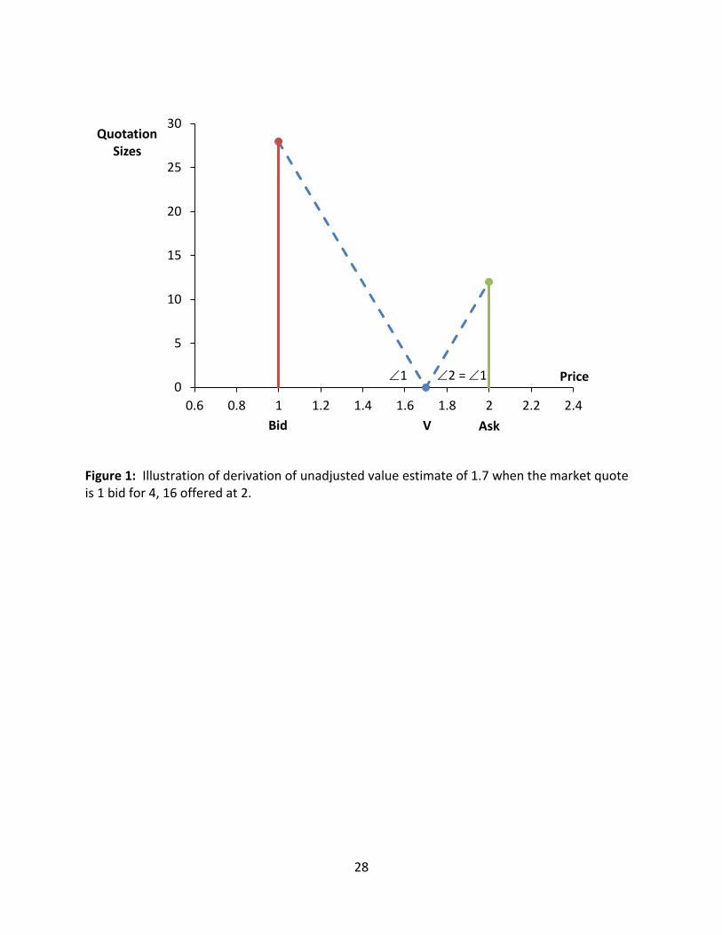
28

Figure 1: Illustration of derivation of unadjusted value estimate of 1.7 when the market quote is 1 bid for 4, 16 offered at 2.

V Bid Ask

0

5

10

15

20

25

30

0.6 0.8 1 1.2 1.4 1.6 1.8 2 2.2 2.4

Quotation Sizes

Price 2 = 1 1

29

Figure 2: Illustration of derivation of adjusted value estimate when the market quote is 1 bid for 4, 16 offered at 2. The dashed line shows the derivation based on net bid and ask prices that include a 0.3¢ maker-taker access fee or liquidity rebate. The solid line presents the derivation based only on the quoted prices. It is identical to the line presented in Figure 1. Accounting for the fees paid and rebated increases the estimated value from 1.7¢ to 1.82¢.

V Bid

0

5

10

15

20

25

30

0.6 0.8 1 1.2 1.4 1.6 1.8 2 2.2 2.4

Quotation Sizes

Price

Ask+0.3¢ Bid-0.3¢

-0.3¢

+0.3¢

V' Ask

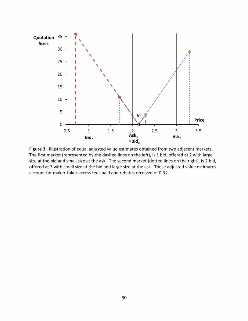
30

Figure 3: Illustration of equal adjusted value estimates obtained from two adjacent markets. The first market (represented by the dashed lines on the left), is 1 bid, offered at 2 with large size at the bid and small size at the ask. The second market (dotted lines on the right), is 2 bid, offered at 3 with small size at the bid and large size at the ask. These adjusted value estimates account for maker-taker access fees paid and rebates received of 0.3¢.

V'

0

5

10

15

20

25

30

35

0.5 1 1.5 2 2.5 3 3.5

Quotation Sizes

Price

Ask2 Ask1

=Bid2 Bid1

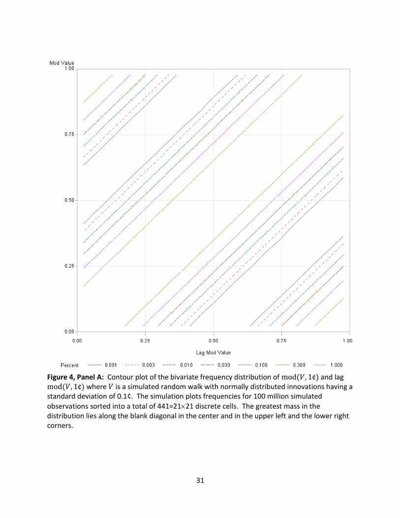
31

Figure 4, Panel A: Contour plot of the bivariate frequency distribution of ( ) and lag ( ) where is a simulated random walk with normally distributed innovations having a standard deviation of 0.1¢. The simulation plots frequencies for 100 million simulated

observations sorted into a total of 441=2121 discrete cells. The greatest mass in the distribution lies along the blank diagonal in the center and in the upper left and the lower right corners.

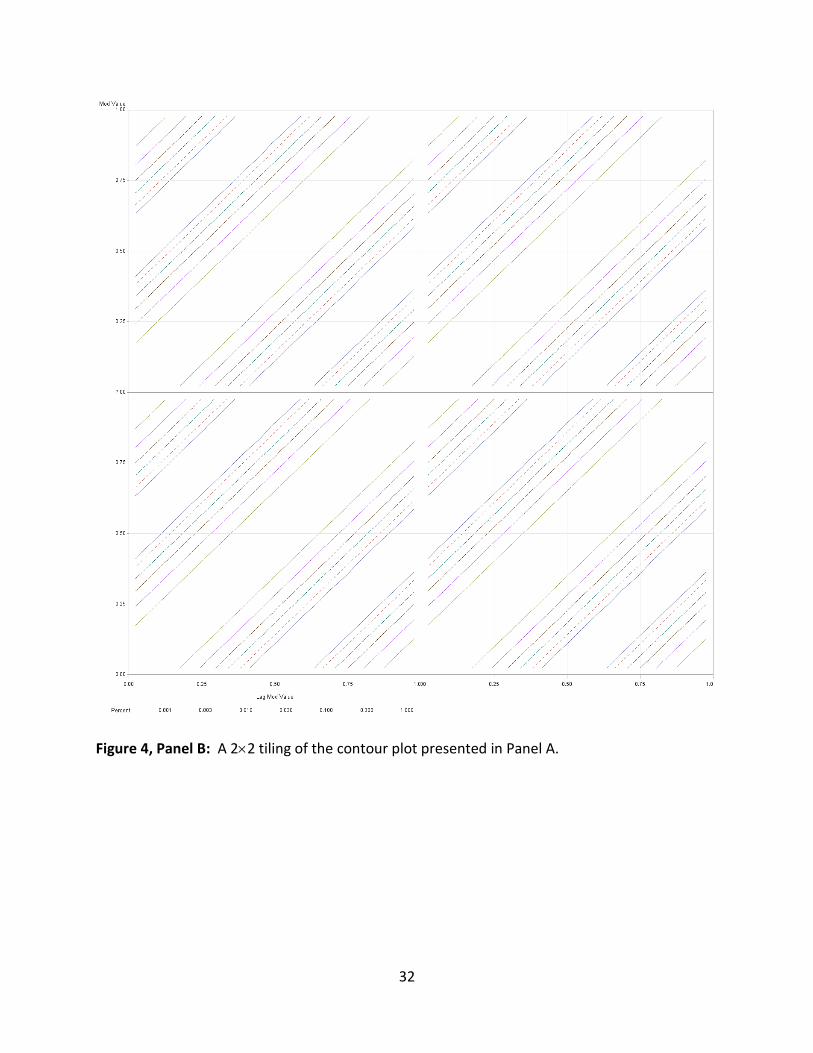
32

Figure 4, Panel B: A 22 tiling of the contour plot presented in Panel A.

33

Figure 5, Panel A: Contour plot of the simulated bivariate sub-penny frequency distribution of the current and lagged unadjusted true value estimates that would be obtained if the access fee and liquidity rebate were 0.275¢. Simulated true value follows a random walk with normally distributed innovations have a standard deviation of 0.1¢. The simulation assumes that the bid-ask spread is 1¢ and that the quotes increase if true value rises above and falls if true value drops below . The bid and ask quote sizes are set so that the adjusted true value estimate is always equal to true value. The plot represents frequencies for 100

million simulated observations sorted into 441=2121 discrete cells. The greatest mass of the distribution lies inside the oval in the center and to a much lesser extent in the two bulges on the left and right. Overlaid on the plot is a 4x4 grid with four cells marked “T” for test and “C” for control. Asymmetry in the distribution can be tested by contrasting the frequencies in the test regions to those in the control regions.

Percent 0.001 0.003 0.010 0.0300.100 0.300 1.000

Sub-pennies

0.0

0.1

0.2

0.3

0.4

0.5

0.6

0.7

0.8

0.9

1.0

Lag Sub-pennies

0.0 0.1 0.2 0.3 0.4 0.5 0.6 0.7 0.8 0.9 1.0

34

Figure 5, Panel B: A contour plot of the same data presented in Panel A in which the horizontal axis plots the sub-penny from which the value changed (as before) and the vertical axis plots the current value estimate minus the integer of its lagged value. This figure has three regions. The middle region consists of value and lagged value estimates obtained from the same market. The upper and lower panels respectively consist of value estimates obtained from a market one tick higher and one tick lower than the previous value estimate. The center region shows the oval distribution while the upper and lower regions show where the budges came from. The bivariate distribution in Panel A is composed of the sums of the densities in these three regions.

Value Estimate

-1.00

-0.75

-0.50

-0.25

0.00

0.25

0.50

0.75

1.00

1.25

1.50

1.75

2.00

Lag Sub-pennies

0.00 0.25 0.50 0.75 1.00

35

Figure 6: Relation between trade initiator and sub-penny of the unadjusted value estimate in markets with 1¢ spreads. All trades that occurred in one-tick markets are identified by their price in relation to the bid and ask that stood at least one second before the trade based on the

continuous indicator variable where

takes the value of 1 if the trade

took place at the ask and -1 if it took place at the bid. This figure plots the average within 20 equally spaced regions of the associated value estimate sub-pennies. The averages are first computed for each security and the results are then averaged across securities using average dollar trade volume weights.

Trade Initiator

-1.00

-0.75

-0.50

-0.25

0.00

0.25

0.50

0.75

1.00

Sub-pennies

0.0 0.1 0.2 0.3 0.4 0.5 0.6 0.7 0.8 0.9 1.0

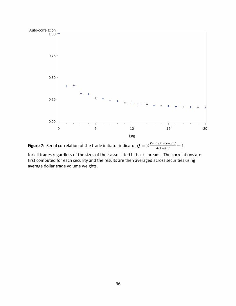
36

Figure 7: Serial correlation of the trade initiator indicator

for all trades regardless of the sizes of their associated bid-ask spreads. The correlations are first computed for each security and the results are then averaged across securities using average dollar trade volume weights.

Auto-correlation

0.00

0.25

0.50

0.75

1.00

Lag

0 5 10 15 20

37

Figure 8, Panel A: Histogram of adjusted value estimate sub-pennies observed in markets with one-tick (1¢) spreads. The horizontal line is the level that would be expected if the data were uniformly distributed. The dashed vertical lines are placed at approximately 0.355¢ and 0.645¢. Between these lines, theory predicts that the distribution should be uniform.

38

Figure 8, Panel B: Probability-probability plot of the unadjusted value estimate distribution that appears in Panel A. The points would plot on the diagonal line if the data were uniformly distributed.

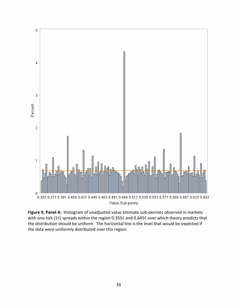
39

Figure 9, Panel A: Histogram of unadjusted value estimate sub-pennies observed in markets with one-tick (1¢) spreads within the region 0.355¢ and 0.645¢ over which theory predicts that the distribution should be uniform. The horizontal line is the level that would be expected if the data were uniformly distributed over this region.

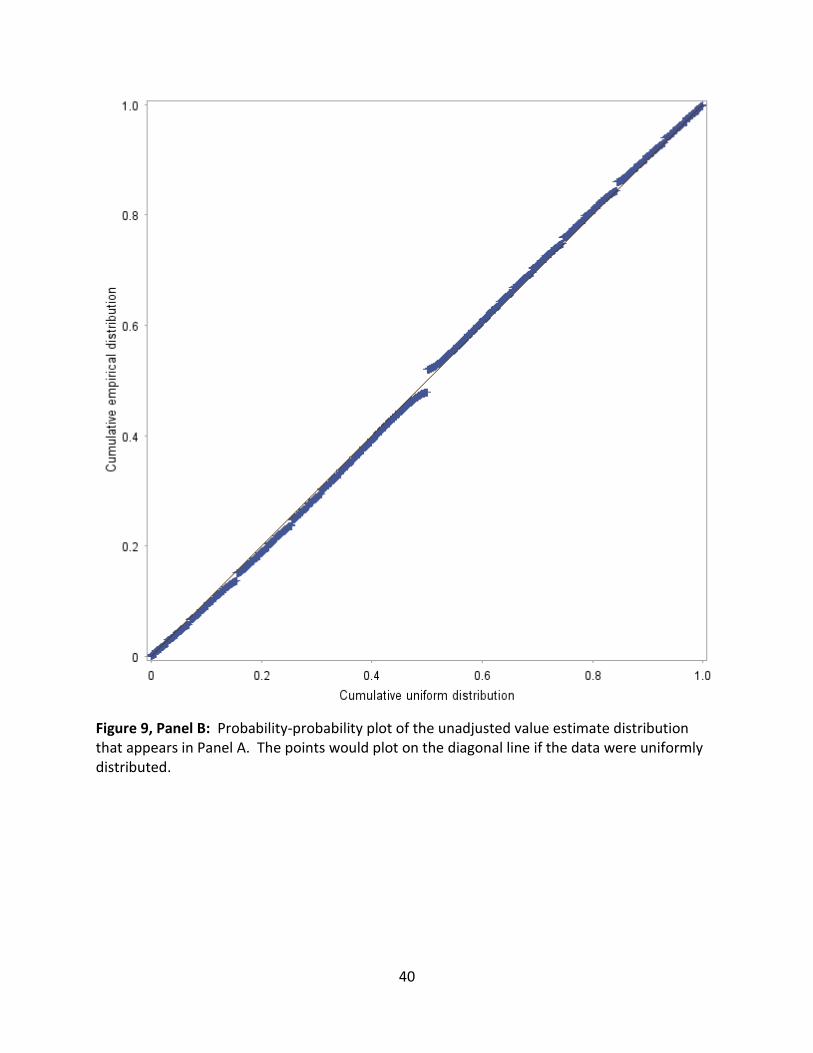
40

Figure 9, Panel B: Probability-probability plot of the unadjusted value estimate distribution that appears in Panel A. The points would plot on the diagonal line if the data were uniformly distributed.

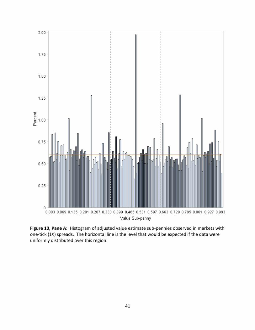
41

Figure 10, Pane A: Histogram of adjusted value estimate sub-pennies observed in markets with one-tick (1¢) spreads. The horizontal line is the level that would be expected if the data were uniformly distributed over this region.

42

Figure 10, Panel B: Probability-probability plot of the adjusted value estimate distribution that appears in Panel A. The points would plot on the diagonal line if the data were uniformly distributed.

43

Figure 11, Panel A: Average contour plot of the bivariate sub-penny frequency distribution of the current and lagged unadjusted true value estimates. The plot represents frequencies

computed from 2,052,686 observations sorted into a total of 441=2121 discrete cells. The frequencies were computed by stock and then averaged across the 81 stocks in the sample weighting by average dollar trading volume.

Percent 0.001 0.003 0.010 0.0300.100 0.300 1.000

Sub-pennies

0.0

0.1

0.2

0.3

0.4

0.5

0.6

0.7

0.8

0.9

1.0

Lag Sub-pennies

0.0 0.1 0.2 0.3 0.4 0.5 0.6 0.7 0.8 0.9 1.0

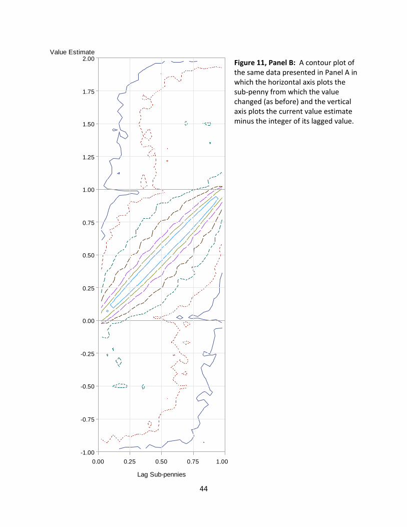
44

Figure 11, Panel B: A contour plot of the same data presented in Panel A in which the horizontal axis plots the sub-penny from which the value changed (as before) and the vertical axis plots the current value estimate minus the integer of its lagged value.

Value Estimate

-1.00

-0.75

-0.50

-0.25

0.00

0.25

0.50

0.75

1.00

1.25

1.50

1.75

2.00

Lag Sub-pennies

0.00 0.25 0.50 0.75 1.00

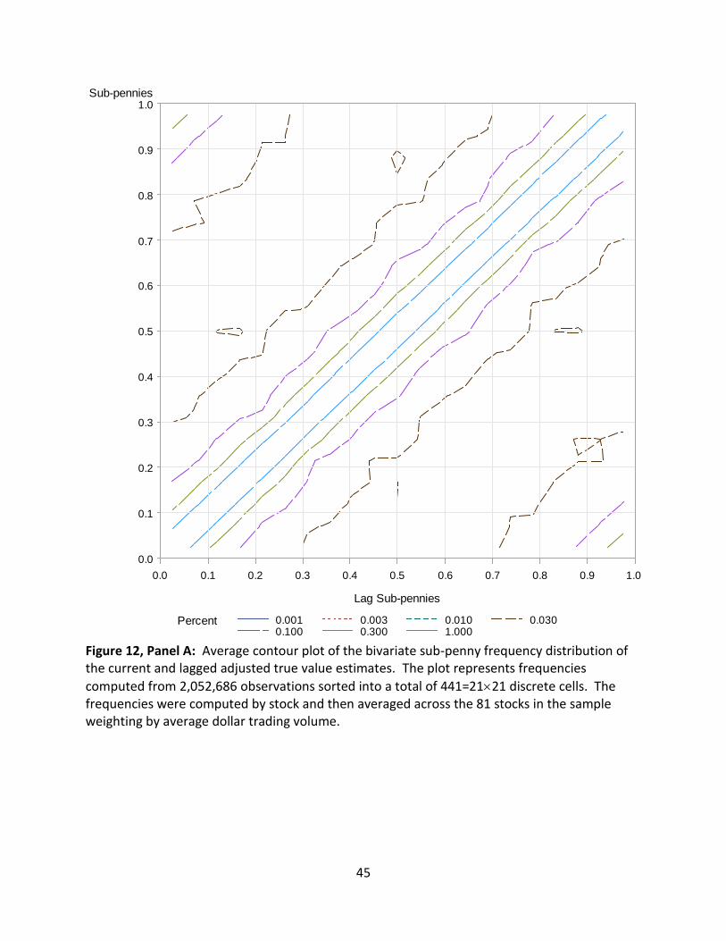
45

Figure 12, Panel A: Average contour plot of the bivariate sub-penny frequency distribution of the current and lagged adjusted true value estimates. The plot represents frequencies

computed from 2,052,686 observations sorted into a total of 441=2121 discrete cells. The frequencies were computed by stock and then averaged across the 81 stocks in the sample weighting by average dollar trading volume.

Percent 0.001 0.003 0.010 0.0300.100 0.300 1.000

Sub-pennies

0.0

0.1

0.2

0.3

0.4

0.5

0.6

0.7

0.8

0.9

1.0

Lag Sub-pennies

0.0 0.1 0.2 0.3 0.4 0.5 0.6 0.7 0.8 0.9 1.0

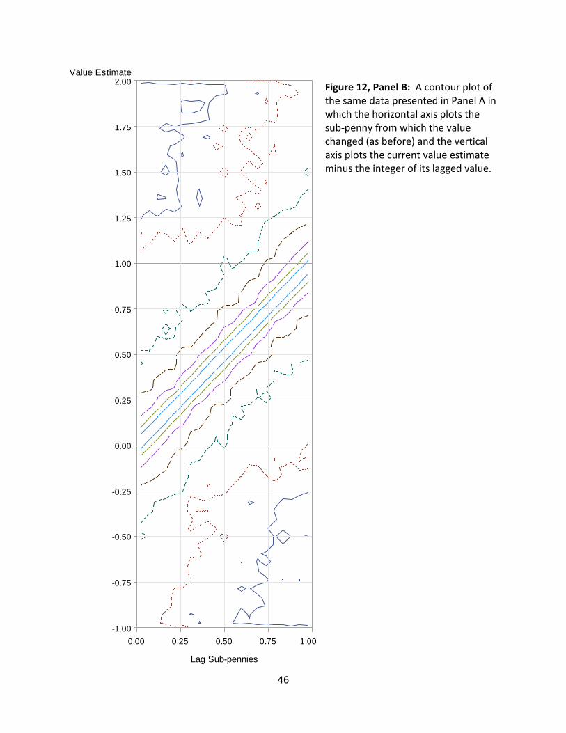
46

Figure 12, Panel B: A contour plot of the same data presented in Panel A in which the horizontal axis plots the sub-penny from which the value changed (as before) and the vertical axis plots the current value estimate minus the integer of its lagged value.

Value Estimate

-1.00

-0.75

-0.50

-0.25

0.00

0.25

0.50

0.75

1.00

1.25

1.50

1.75

2.00

Lag Sub-pennies

0.00 0.25 0.50 0.75 1.00

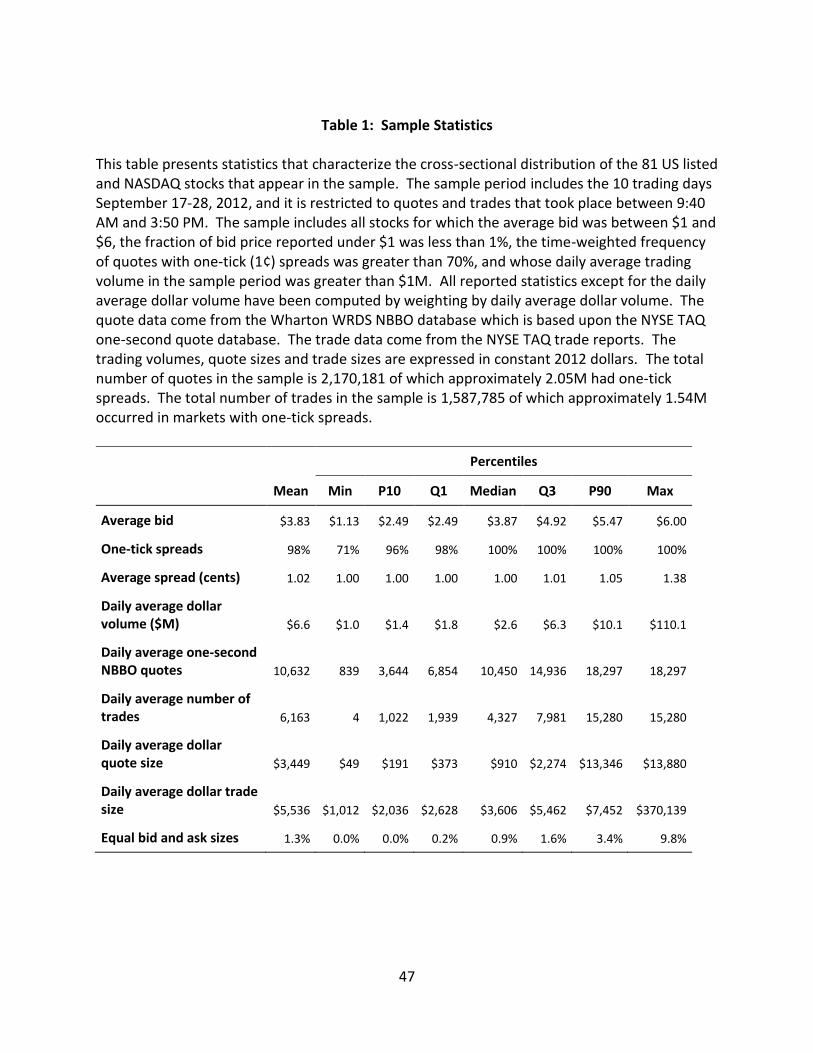
47

Table 1: Sample Statistics

This table presents statistics that characterize the cross-sectional distribution of the 81 US listed and NASDAQ stocks that appear in the sample. The sample period includes the 10 trading days September 17-28, 2012, and it is restricted to quotes and trades that took place between 9:40 AM and 3:50 PM. The sample includes all stocks for which the average bid was between $1 and $6, the fraction of bid price reported under $1 was less than 1%, the time-weighted frequency of quotes with one-tick (1¢) spreads was greater than 70%, and whose daily average trading volume in the sample period was greater than $1M. All reported statistics except for the daily average dollar volume have been computed by weighting by daily average dollar volume. The quote data come from the Wharton WRDS NBBO database which is based upon the NYSE TAQ one-second quote database. The trade data come from the NYSE TAQ trade reports. The trading volumes, quote sizes and trade sizes are expressed in constant 2012 dollars. The total number of quotes in the sample is 2,170,181 of which approximately 2.05M had one-tick spreads. The total number of trades in the sample is 1,587,785 of which approximately 1.54M occurred in markets with one-tick spreads.

Mean

Percentiles

Min P10 Q1 Median Q3 P90 Max

Average bid $3.83 $1.13 $2.49 $2.49 $3.87 $4.92 $5.47 $6.00

One-tick spreads 98% 71% 96% 98% 100% 100% 100% 100%

Average spread (cents) 1.02 1.00 1.00 1.00 1.00 1.01 1.05 1.38

Daily average dollar volume ($M) $6.6 $1.0 $1.4 $1.8 $2.6 $6.3 $10.1 $110.1

Daily average one-second NBBO quotes 10,632 839 3,644 6,854 10,450 14,936 18,297 18,297

Daily average number of trades 6,163 4 1,022 1,939 4,327 7,981 15,280 15,280

Daily average dollar quote size $3,449 $49 $191 $373 $910 $2,274 $13,346 $13,880

Daily average dollar trade size $5,536 $1,012 $2,036 $2,628 $3,606 $5,462 $7,452 $370,139

Equal bid and ask sizes 1.3% 0.0% 0.0% 0.2% 0.9% 1.6% 3.4% 9.8%

48

Table 2, Panel A: Average Return Correlations among Stocks This table presents average return correlation coefficients for all pairs of stocks in the sample measured at various intraday intervals. There are 3,240 pairs of the 81 stocks in the sample. The returns are computed from three different estimates of value. The quote midpoint returns are estimated from the average of the bid and ask quotes. The unadjusted returns are estimated as a quotation size-weighted average of bid and ask prices using the formula in equation (2). The adjusted returns are quotation size-weighted averages of bid and ask prices that adjust for maker-taker fees using equation (6).

Time interval Return estimate type Assumed maker-taker fee Average correlation

coefficient

1s Quote midpoint 0.29%

Unadjusted 0¢ 0.47%

Adjusted 0.275¢ 0.55%

5s Quote midpoint 0.78%

Unadjusted 0¢ 1.09%

Adjusted 0.275¢ 1.17%

10s Quote midpoint 1.22%

Unadjusted 0¢ 1.59%

Adjusted 0.275¢ 1.67%

20s Quote midpoint 1.93%

Unadjusted 0¢ 2.33%

Adjusted 0.275¢ 2.38%

30s Quote midpoint 2.44%

Unadjusted 0¢ 2.90%

Adjusted 0.275¢ 2.93%

60s Quote midpoint 3.65%

Unadjusted 0¢ 4.04%

Adjusted 0.275¢ 4.00%

49

Table 2, Panel B: Paired t-tests for Differences in Average Return Correlations among Stocks This table presents mean differences for the average correlation coefficients reported in Panel B between return values based on the three return estimates. The t-value is for the paired t-tests of the significance of the test. The t-statistic does not have the standard Student-t distribution under the null of no difference because the ( ) different pairwise correlations are not independent. A bootstrap analysis indicates that the reported t-values are all statistically significant at the 0.01 significance level.

Time interval Contrast Mean

difference t-Value

1s Unadjusted minus Quote midpoint 0.18% 31.3

Adjusted minus Unadjusted 0.07% 27.4

Adjusted minus Quote midpoint 0.26% 32.0

5s Unadjusted minus Quote midpoint 0.31% 28.7

Adjusted minus Unadjusted 0.08% 18.9

Adjusted minus Quote midpoint 0.39% 27.6

10s Unadjusted minus Quote midpoint 0.37% 26.6

Adjusted minus Unadjusted 0.08% 14.1

Adjusted minus Quote midpoint 0.45% 24.8

20s Unadjusted minus Quote midpoint 0.41% 24.3

Adjusted minus Unadjusted 0.04% 6.7

Adjusted minus Quote midpoint 0.45% 20.8

30s Unadjusted minus Quote midpoint 0.46% 24.5

Adjusted minus Unadjusted 0.03% 4.1

Adjusted minus Quote midpoint 0.49% 20.0

60s Unadjusted minus Quote midpoint 0.39% 18.0

Adjusted minus Unadjusted ( 0.04%) -4.2

Adjusted minus Quote midpoint 0.35% 12.1

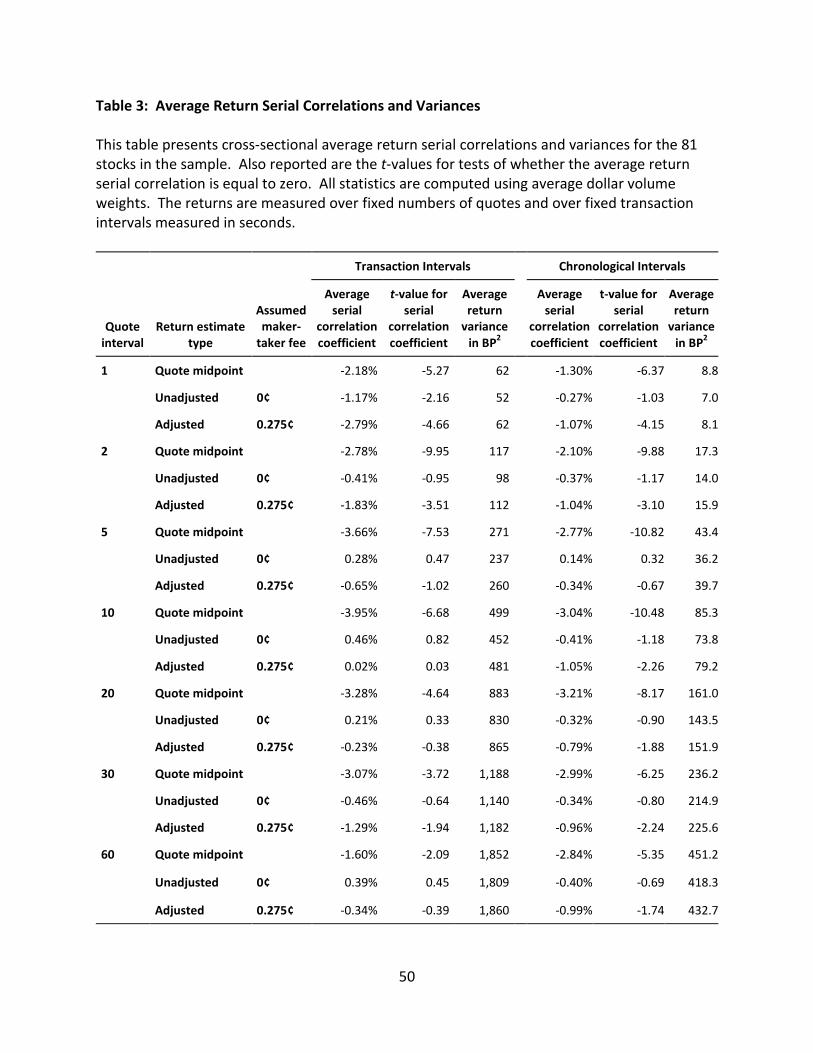
50

Table 3: Average Return Serial Correlations and Variances This table presents cross-sectional average return serial correlations and variances for the 81 stocks in the sample. Also reported are the t-values for tests of whether the average return serial correlation is equal to zero. All statistics are computed using average dollar volume weights. The returns are measured over fixed numbers of quotes and over fixed transaction intervals measured in seconds.

Transaction Intervals Chronological Intervals

Quote interval

Return estimate type

Assumed maker-

taker fee

Average serial

correlation coefficient

t-value for serial

correlation coefficient

Average return

variance in BP

2

Average serial

correlation coefficient

t-value for serial

correlation coefficient

Average return

variance in BP

2

1 Quote midpoint -2.18% -5.27 62 -1.30% -6.37 8.8

Unadjusted 0¢ -1.17% -2.16 52 -0.27% -1.03 7.0

Adjusted 0.275¢ -2.79% -4.66 62 -1.07% -4.15 8.1

2 Quote midpoint -2.78% -9.95 117 -2.10% -9.88 17.3

Unadjusted 0¢ -0.41% -0.95 98 -0.37% -1.17 14.0

Adjusted 0.275¢ -1.83% -3.51 112 -1.04% -3.10 15.9

5 Quote midpoint -3.66% -7.53 271 -2.77% -10.82 43.4

Unadjusted 0¢ 0.28% 0.47 237 0.14% 0.32 36.2

Adjusted 0.275¢ -0.65% -1.02 260 -0.34% -0.67 39.7

10 Quote midpoint -3.95% -6.68 499 -3.04% -10.48 85.3

Unadjusted 0¢ 0.46% 0.82 452 -0.41% -1.18 73.8

Adjusted 0.275¢ 0.02% 0.03 481 -1.05% -2.26 79.2

20 Quote midpoint -3.28% -4.64 883 -3.21% -8.17 161.0

Unadjusted 0¢ 0.21% 0.33 830 -0.32% -0.90 143.5

Adjusted 0.275¢ -0.23% -0.38 865 -0.79% -1.88 151.9

30 Quote midpoint -3.07% -3.72 1,188 -2.99% -6.25 236.2

Unadjusted 0¢ -0.46% -0.64 1,140 -0.34% -0.80 214.9

Adjusted 0.275¢ -1.29% -1.94 1,182 -0.96% -2.24 225.6

60 Quote midpoint -1.60% -2.09 1,852 -2.84% -5.35 451.2

Unadjusted 0¢ 0.39% 0.45 1,809 -0.40% -0.69 418.3

Adjusted 0.275¢ -0.34% -0.39 1,860 -0.99% -1.74 432.7