Makeup-Go: Blind Reversion of Portrait Edit∗

Ying-Cong Chen1 Xiaoyong Shen2 Jiaya Jia1,21The Chinese University of Hong Kong 2Tencent Youtu Lab

ycchen@cse.cuhk.edu.hk dylanshen@tencent.com leojia9@gmail.com

Abstract

Virtual face beautification (or markup) becomes commonoperations in camera or image processing Apps, which isactually deceiving. In this paper, we propose the task ofrestoring a portrait image from this process. As the firstattempt along this line, we assume unknown global opera-tions on human faces and aim to tackle the two issues of skinsmoothing and skin color change. These two tasks, intrigu-ingly, impose very different difficulties to estimate subtle de-tails and major color variation. We propose a ComponentRegression Network (CRN) and address the limitation of us-ing Euclidean loss in blind reversion. CRN maps the editedportrait images back to the original ones without knowingbeautification operation details. Our experiments demon-strate effectiveness of the system for this novel task.

1. IntroductionPopularity of social networks of Facebook, Snapchat,

and Instagram, and the fast development of smart phonesmake it fun to share portraits and selfies online. This trendalso motivates the development of widely used proceduresto automatically beautify faces. The consequence is thatmany portraits found online are good looking, but not real.In this paper, we propose the task of blind reverse of thisunknown beautification process and restore faces similar towhat are captured by cameras. We call this task portraitbeautification reversion, or makeup-go for short.

Scope of Application Virtual beautification is performedquite differently in software, which makes it impossible tolearn all operations that can be performed to smooth skin,suppress wrinkle and freckle, adjust tone, to name a few.To make the problem trackable in a well-constrained space,we learn from data the automatic process for particular soft-ware and then restore images output from it without know-ing the exact algorithms. Also, we assume subtle cues stillexists after virtual beutification, even if they are largely sup-

∗This work is in part supported by a grant from the Research GrantsCouncil of the Hong Kong SAR (project No. 413113).

pressed. Also, at this moment, we do not handle geometrictransformation for face-lift.

Difficulty of Existing Solutions Existing restorationwork [36, 32, 28, 30] only handles reversion of knownand/or linear operations. There is no mature study yetwhat if several unknown nonlinear operations are coupledfor restoration. The strategy of [11] is to infer the sequenceof operations and then each of them. We however note thisscheme does not work in our task for complicated beautifi-cation without knowing candidate operations.

In addition, directly learning reversion by deep neu-ral networks is not trivial. Previous CNN frameworksonly address particular tasks of super-resolution [7, 8, 13],noise/artifact removal [6], image filtering [18], etc. Learn-ing in these tasks are with some priors, such as the upsam-pling factors, noise patterns, and filter parameters. Our taskmay not give such information and needs to be general.

In terms of network structures, most low-level visionframeworks stack layers of convolution and nonlinear rec-tification for regression of the Euclidean loss. This type ofloss is useful for previous tasks such as denoise [6]. Butthey are surprisingly not applicable to our problem becauselevels of complex changes make it hard to train a network.We analyze this difficulty below.

Challenge in Our Blind Reversion To show the limita-tion of existing CNN in our task, we apply state-of-the-art VDSR [14], FSRCNN [8] and PSPNet [8], to directlyregress the data after edit. VDSR performs the best amongthe three. It is an image-to-image regression network withL2 loss that achieves high PSNRs in super-resolution. Itsuccessfully learns large-scale information such as skincolor and illumination, as shown in Figure 1.

It is however intriguing to note that many details, espe-cially the region that contains small freckles and wrinkles,are not well recovered in the final output. In fact, VDSR isalready a deep model with 20 layers – stacking more lay-ers in our experiments does not help regress these subtleinformation. This manifests that the network capacity is notthe bottleneck. The main problem, actually, is on employ-ment of the Euclidean loss that makes detailed changes be

1

(a) Edited Image (b) CNN (c) Output (d) Groundtruth (e) Close-up

Figure 1. Illustration of using existing CNNs for portrait beautification reversion. (a) is the image edited by Photoshop Express; (b)represents a CNN network for image regression; (c) is the output of the network; (d) is the ground truth image; (e) is the close-up patchescropped from the edited image, output and ground truth image. It cannot achieve good performance on face detail recovery.

ignored. This is not desirable to our task since the main ob-jective is exactly to restore these small details on faces. Ig-noring them would completely fail operation reversal. Weprovide more analysis in Section 3, which gives the idea ofconstructing our Component Regression Network (CRN).

Our Contributions We design a new network structureto address above elaborated detail diminishing issues andhandle both coarse and subtle components reliably. Insteadof directly regressing the images towards the unedited ver-sion, our network regresses levels of principal componentsof the edited parts separately. As a result, subtle detail in-formation would not be ignored. It can now be similarlyimportant as strong patterns in final image reconstruction,and thus is guaranteed to get lifted in regression. Our con-tribution in this paper is threefold.

• We propose the task of general blind reversion for por-trait edit or other inverse problems.

• We discover and analyze the component dominationeffect in blind reversion and ameliorate it with a newcomponent-based network architecture.

• Extensive analysis and experiments prove the effec-tiveness of our model.

2. Related Work

We in this section review related image editing tech-niques and the convolutional neural networks (CNNs) forimage processing.

Image Editing Image editing is a big area. Useful toolsinclude those for image filtering [19, 3, 9, 29, 35, 10], retar-geting [23, 1], composition [21], completion [2, 5], noise re-moval [22, 27], and image enhancement [33]. Most of theseoperations are not studied for their reversibility. Only thework of [11] recovers image editing history assuming thatcandidate editing operations are known in advance, which

is not applicable to our case where unknown edit comes outfrom commercial software.

CNNs for Image Regression Convolutional neural net-works are effective now to solve the regression problem inimage processing [8, 14, 7, 30, 17, 31]. In these methods,the Euclidean loss is usually employed. In [31], Euclideanloss in gradient domain is used to capture strong edge in-formation for filter learning. This strategy does not fit ourproblem since many details do not contain strong edges.

Our method is also related to the perception loss basedCNNs [13, 16], which are recently proposed for style trans-fer and super-resolution. In [13], perception loss is definedas the Euclidean distance between features extracted by dif-ferent layers of an ImageNet [15] pretrained VGG network[25]. The insight is that layers of the pretrained networkcapture levels of information in edges, texture or even ob-ject parts [34]. In [16], an additional adversarial part is in-corporated to encourage the output to reside on the manifoldof target dataset. However, as explained in [13, 16], percep-tional loss produces lower PSNR results than the Euclideanone. Since the perception loss is complex, it is difficult toknow what component is not regressed well. Our approachdoes not use this loss accordingly.

3. Elaboration of Challenges

As shown in Figure 1, our blind reversion system needsto restore several levels of details. When directly applyingthe methods of [14], many details are still missing even ifPSNRs are already reasonable, as shown in Figure 1(c,e).We intriguingly found that the main reason is on the choiceof Euclidean loss function [8, 14, 7, 30, 17] for this regres-sion task, which is used to measure the difference betweenthe network output and target. Perception loss [13, 16], al-ternatively, is used for remedying details at the cost of sac-rificing PSNRs, i.e., overall fidelity to the target images.

In this section, we explain our finding that Euclidean loss

(a) Edited Image

(b) Relative Improvement

(c) Close-up (d) Original Image

10 20 30 40 50 60 70 80 90 100 110 120

0

0.2

0.4

0.6

0.8

1 Ours

VDSR

Groundtruth

Rel

ativ

e Im

pro

vem

ent

Component

Figure 2. Relative improvement of different principal components. (a) and (d) are the edited and ground truth images respectively. (b)shows the relative similarity improvement of different principal components regarding network output. (c) shows close-up patches withappearance change using only the top 1, 2, 3, 5, 10, 20, 50 and 100 components. Best viewed in color.

cannot let network learn details well due to the componentdomination effect. We take the VDSR network [14] as anexample, which uses Euclidean loss and achieves state-of-the-art results in super-resolution. So it already has the goodability for detail regression. When applied to our task, itdoes not produces many details, as illustrated in Figure 1.

Improvement Measure Regarding Levels of Details Tounderstand this process, we analyze the difference betweenthe network output and the ground truth image regardingdifferent principal components, which is shown in Figure 2.Our computation is explained below.

We denote the edited input and unedited ground truthimage as IX and IY , and the network output as IZ . Wecompute the discrepancy maps as Ie = IY − IX andIe = IY − IZ on collected 107 patches where each patchis with size 11 × 11. These patches are vectorized wherePCA coefficients U = {u1, u2, · · · , um2} are extractedfrom them in a descending order. Then eij = uTi vj andeij = uTi vj denote the ith components of the jth discrep-ancy patches, where vj and vj are the vectorized patches.The final improvement measure of the ith PCA componentbetween the network output and the ground truth image isexpressed as

di =

∑j(e

2ij − e2ij)∑j e

2ij

. (1)

When the network output is exactly the ground truth, di = 1for all i, which is the red dash line in Figure 2(b). A large diindicates that the network regresses the ith component well.

Relative Improvement Analysis As shown in Figure 2(the cyan curve), VDSR achieves high di for the top-rankingcomponents. Intriguingly the performance drops dramati-cally for other smaller ones. As shown in Figure 2(c), thelower-ranking components mostly correspond to details of

faces, such as freckles. Their unsuccessful reconstructiongreatly affects our blind reversion task where details are thevital visual factors.

The main reason that VDSR fails to regress low-rankingcomponents is the deployment of the Euclidean loss, whichis mainly controlled by the largest principal components.This loss is expressed as

J =1

2m2||F (vX)− vY ||2, (2)

where vX ∈ Rm2×1 is the input edited image patch, F (·) ∈Rm2×1 is mapping function defined by the network, andvY ∈ Rm2×1 is the target image patch.

Note that the PCA base matrix U satisfies UUT = I ,where I is an identity matrix. Thus projecting F (vX) andvY to U does not change the loss J , i.e.,

J =1

2m2||UTF (vX)− UT vY ||2

=1

2m2

m2∑i=1

||fi(vX)− uivY ||2,(3)

where fi(vX) = uTi F (vX). In this regard, J can be viewedas a sum of different objectives that regress components ofthe target image patches. Since these components are ex-tracted by PCA, there is limited information shared amongdifferent principal components.

Note that the variance of those components differsgreatly. As shown in Figure 3, the eigenvalues for the first afew components are much larger than others and the top5 components contribute more than 99% variance. Thismakes the Euclidean loss function dominated by the majorones, while other components can be safely ignored duringregression, causing the component domination effect.

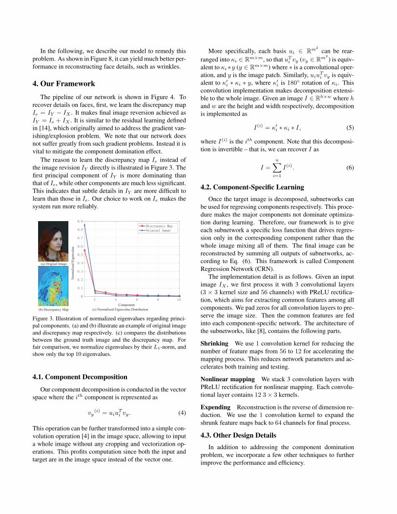
In the following, we describe our model to remedy thisproblem. As shown in Figure 8, it can yield much better per-formance in reconstructing face details, such as wrinkles.

4. Our Framework

The pipeline of our network is shown in Figure 4. Torecover details on faces, first, we learn the discrepancy mapIe = IY − IX . It makes final image reversion achieved asIY = Ie + IX . It is similar to the residual learning definedin [14], which originally aimed to address the gradient van-ishing/explosion problem. We note that our network doesnot suffer greatly from such gradient problems. Instead it isvital to mitigate the component domination effect.

The reason to learn the discrepancy map Ie instead ofthe image revision IY directly is illustrated in Figure 3. Thefirst principal component of IY is more dominating thanthat of Ie, while other components are much less significant.This indicates that subtle details in IY are more difficult tolearn than those in Ie. Our choice to work on Ie makes thesystem run more reliably.

(a) Original Image

(b) Discrepancy Map

Component

No

rmal

ized

Eig

env

alu

e

(c) Normalized Eigenvalue Distribution

Figure 3. Illustration of normalized eigenvalues regarding princi-pal components. (a) and (b) illustrate an example of original imageand discrepancy map respectively. (c) compares the distributionsbetween the ground truth image and the discrepancy map. Forfair comparison, we normalize eigenvalues by their L1-norm, andshow only the top 10 eigenvalues.

4.1. Component Decomposition

Our component decomposition is conducted in the vectorspace where the ith component is represented as

vy(i) = uiu

Ti vy. (4)

This operation can be further transformed into a simple con-volution operation [4] in the image space, allowing to inputa whole image without any cropping and vectorization op-erations. This profits computation since both the input andtarget are in the image space instead of the vector one.

More specifically, each basis ui ∈ Rm2

can be rear-ranged into κi ∈ Rm×m, so that uTi vy (vy ∈ Rm2

) is equiv-alent to κi ∗y (y ∈ Rm×m) where ∗ is a convolutional oper-ation, and y is the image patch. Similarly, uiuTi vy is equiv-alent to κ′i ∗ κi ∗ y, where κ′i is 180◦ rotation of κi. Thisconvolution implementation makes decomposition extensi-ble to the whole image. Given an image I ∈ Rh×w where hand w are the height and width respectively, decompositionis implemented as

I(i) = κ′i ∗ κi ∗ I, (5)

where I(i) is the ith component. Note that this decomposi-tion is invertible – that is, we can recover I as

I =

n∑i=1

I(i). (6)

4.2. Component-Specific Learning

Once the target image is decomposed, subnetworks canbe used for regressing components respectively. This proce-dure makes the major components not dominate optimiza-tion during learning. Therefore, our framework is to giveeach subnetwork a specific loss function that drives regres-sion only in the corresponding component rather than thewhole image mixing all of them. The final image can bereconstructed by summing all outputs of subnetworks, ac-cording to Eq. (6). This framework is called ComponentRegression Network (CRN).

The implementation detail is as follows. Given an inputimage IX , we first process it with 3 convolutional layers(3 × 3 kernel size and 56 channels) with PReLU rectifica-tion, which aims for extracting common features among allcomponents. We pad zeros for all convolution layers to pre-serve the image size. Then the common features are fedinto each component-specific network. The architecture ofthe subnetworks, like [8], contains the following parts.

Shrinking We use 1 convolution kernel for reducing thenumber of feature maps from 56 to 12 for accelerating themapping process. This reduces network parameters and ac-celerates both training and testing.

Nonlinear mapping We stack 3 convolution layers withPReLU rectification for nonlinear mapping. Each convolu-tional layer contains 12 3× 3 kernels.

Expending Reconstruction is the reverse of dimension re-duction. We use the 1 convolution kernel to expand theshrunk feature maps back to 64 channels for final process.

4.3. Other Design Details

In addition to addressing the component dominationproblem, we incorporate a few other techniques to furtherimprove the performance and efficiency.

1 !subnetwork

2"#subnetwork

shared subnetwork

Common network

PCA

Component Decomposition

$%

$Z

…

… SUM

supervise

$& ' $%

Figure 4. Our CRN Pipeline. CRN learns the discrepancy map Ie = IY −IX . It is further decomposed into different components accordingto Eq. (5) to supervise each subnetwork. During testing, we feed the network with an edited image where each subnetwork outputs thecorresponding component. We sum network output to obtain the final result.

(a) Portrait samples (b) Effect of edit

Figure 5. Examples in our dataset. (a) shows a few samples in our dataset. (b) shows the effect of edit. The 4 images are the original image,and images edited by MT, PS and INS respectively.

Subnetwork Sharing One critical factor that influencesperformance is the number of subnetworks. Ideally, itshould equal to the number of pixels of an image patch.However, allocating one subnetwork to each component isnot affordable considering the computation cost. As illus-trated in Figure 3, very low-ranking components are withsimilar variance. This finding inspires us to empirically useonly 7 subnetworks to regress the top 7 components. Thereis one last shared subnetwork to regress all remaining com-ponents. This strategy works quite well in our task. It savesa lot of computation while not much affecting result quality.

Scale Normalization Practically, the lower-ranked com-ponents have small variance, making gradients easily domi-nated by higher-ranked ones in the shared network. To solvethis problem, each component is divided by its correspond-ing standard deviation, i.e., I(i)norm = 1√

λiI(i) where I(i) is

defined in Eq. (5) and λi is the ith eigenvalue. With this op-eration, all components have similar scales. During testing,we scale the subnetwork output back to the required quan-tity by multiplying corresponding standard deviation beforesumming them up.

5. Experimental SettingsImplementation setting All CRN models have the samenetwork architecture described in Section 4. Unless other-

wise stated, our models use 7 subnetworks to regress thetop 7 components, and take a shared subnetwork to regressothers. Our models are implemented in Caffe [12]. Duringtraining, the initial learning rate is 0.01. It decreases follow-ing a polynomial policy with 40,000 iterations. Gradientclipping [20, 14] is also used to avoid gradient explosion,so that large learning rates are allowed.

Dataset We utilized the portrait dataset [24] for evalua-tion. This dataset contains 2,000 images with various age,color, clothing, hair style, etc. We manually select imagesthat contain many details and are not likely to have beenedited before. They form our final dataset. A few examplesare shown in Figure 5(a). These images are referred to asthe ground truth data (not edited) in our experiments. Thenwe use three most popular image editing systems, i.e., Pho-toshop Express (PS), Meitu (MT) and Instagram (INS), toprocess the images. PS and MT are stand-alone software,while INS is photo sharing application that contains built-inediting functions. These systems have many users. Figure5(b) shows editing results of different systems. We trainedour models to reverse edit for each of the three systems.

Evaluation metrics The Peak Signal-to-Noise ratio(PSNR) and structural similarity (SSIM) [26] index are usedfor quantifying the performance of our approach. How-ever, these measures are not sensitive to the details in hu-

(a) Edited Image (b) 2 Component (c) 4 Component (d) 7 Component (e) Ground truth

Figure 6. Visualization of contribution of each branch. (a) is the edited image; (b)-(d) show results using different numbers of branches;(e) is the original image (best viewed in color).

man faces. We thus utilize the relative improvement definedin Eq. (1) to form the Accumulated Relative Improvement(ARI) measure. ARI is set as

ARI =∑i

di, (7)

where di is introduced in Eq. (1). ARI measures the rel-ative improvement over all components. They contributesimilarly to the final result disregarding their initial weightsin eigenvalues.

6. Evaluation of Our Approach

The critical issue for the blind reversion task is the com-ponent domination effect. In the following, we explain theeffectiveness of different steps in our approach.

6.1. Contribution of Component-specific Learning

Statistical evaluation As the main contribution, thecomponent-specific learning mitigates the component dom-ination effect effectively. Table 1 shows PSNR, SSIM andARI for different numbers of branches. When the num-ber of branches is 1, all components are mixed, which be-comes the baseline approach of our model. As the num-ber of branches increases, the performance betters consis-tently, which means the domination effect is gradually sup-pressed. Note that the improvement is large in the beginning(e.g., 76.8% improvement for 2 branches in terms of ARI),and slows down with more branches (e.g., 4.32% with 7branches in terms of ARI). This indicates that componentdomination effect is more severe in high-ranking principalcomponents than low-ranking ones. Thus it is reasonable touse respective branches for major components, and a sharedbranch to regress the rest.

Branch 1 2 3 4 5 6 7PSNR 36.7 39.9 39.0 41.4 41.5 41.6 41.9SSIM 0.96 0.97 0.97 0.98 0.98 0.98 0.98ARI 12.5 22.1 32.4 50.1 53.7 56.1 60.5

Table 1. Evaluation of effectiveness of component-specific learn-ing.

PSNR SSIM ARI

MTFull Model 40.9 0.98 60.5w/o DisMap 39.8 0.98 49.7w/o ScaleNorm 37.4 0.97 -6.0

PSFull Model 33.3 0.95 28.9w/o DisMap 32.9 0.95 20.8w/o ScaleNorm 31.2 0.95 -15.2

INSFull Model 35.9 0.94 12.9w/o DisMap 34.7 0.94 3.5w/o ScaleNorm 32.1 0.93 -25.7

Table 2. Evaluation of effectiveness of discrepancy map learningand scale normalization.

Visualization We further visualize the information thatdifferent branches contribute in Figure 6. As shown in Fig-ure 6(a), face details are largely smoothed by the editingsystem. Then we use our 7-branch CRN model to processit. We block some branch output to understand what eachbranch learns. The result is shown in Figure 6(b-d). Thesmoothed wrinkle becomes more noticeable as the numberof component increases. When all 7 branches are used, evena very subtle freckle can be recovered.

6.2. Contribution of Other Components

In addition to the component-specific learning, scale nor-malization and discrepancy map learning are also very im-

0 20 40 60 80 100 120

Component

0

0.2

0.4

0.6

0.8

1

Rel

ativ

e Im

pro

vem

ent

Ours

VDSR

Perception

Groundtruth

(a) Meitu

0 20 40 60 80 100 120

Component

0

0.2

0.4

0.6

0.8

1

Rel

ativ

e Im

pro

vem

ent

Ours

VDSR

Perception

Groundtruth

(b) Photoshop

0 20 40 60 80 100 120

Component

0

0.2

0.4

0.6

0.8

1

Rel

ativ

e Im

pro

vem

ent

Ours

VDSR

Perception

Groundtruth

(c) Instagram

Figure 7. Results of different methods in the three different datasets.

PSNR SSIM ARI

MTOurs 40.9 0.98 60.5VDSR [14] 39.5 0.96 12.8Perception [16] 28.1 0.96 -83.7

PSOurs 33.3 0.95 28.9VDSR [14] 32.2 0.94 4.2Perception [16] 22.4 0.91 -89.2

INSOurs 35.9 0.94 12.9VDSR [14] 33.4 0.93 4.8Perception [16] 18.7 0.89 -44.2

Table 3. Comparison with VDSR and perception loss on MT, PSand INS.

portant to our model. To evaluate them, in Table 2, wecompare our full model with models that 1) directly regressthe ground truth image (denoted as w/o DisMap); 2) do notperform scale normalization (denoted as w/o ScaleNorm).The quantities in tables indicate that the performance dropswithout discrepancy map learning. This is because directlylearning the original image suffers more severely from thecomponent domination effect. Note that if scale normal-ization is not used, our model fails because the small-scalecomponents are not learned successfully.

6.3. Comparison with Other Methods

There is no exact work addressing blind reversion of un-known image edit. But in a broader context, our modelis related to image-to-image FCN regression. VDSR [14]is an FCN model that achieves state-of-the-art results insuper-resolution where high-frequency information needsto be restored. Our problem is different on the fact that im-age edit can change all levels of information regarding allcoarser and subtle structures, while super-resolution gener-ally keeps the coarse level of edges.

Perception loss [16] is another regression loss function.It is combination of VGG-based content loss and adversar-ial loss. Compared to Euclidean loss, perception loss isperformed in the feature level. As indicated in [13, 16],

it yields better performance on details than Euclidean loss,but achieves lower PSNR.

Real-world Examples Figure 8 compares VDSR [14],perception loss [16], and our model in real-world cases. Itshows that VDSR can regress color and illumination well,and yet fail to learn details. On the contrary, by combiningVGG loss and adversarial loss, perception loss learns de-tails better. But it does not handle color similarly well. Thisis because perception loss utilizes layers of VGG network,which is trained for classification. It requires robust fea-tures invariant to color or small texture change. Our modelhandles both problems for satisfying detail regression.

Statistical Comparison To prove the generality, we fur-ther show PSNR, SSIM and ARI (Eq (7)) over all testingimages edited by MT, PS and INS in Table 3. Statistics in-dicate that our model yields better performance than VDSRand perception loss. It means our model can regress por-traits more accurately.

In addition, benefitted from component-specific learn-ing, our model outperforms other methods in terms of ARIby a large margin. It is a bit surprising that perception lossdoes not perform that well regarding these statistical met-rics, especially the ARI. It actually is because perceptionloss relies on the VGG network [13, 25], which is trained forclassification and may discard information that is not dis-criminative. Thus these components would be completelyignored by the network. The adversarial part does not helpfind them since it does not impose similarity between thenetwork output and the target. As will be shown later, per-ception loss works well on certain components, but not allof them.

Component Level Comparison In addition to the statis-tic metrics, it is also interesting to see relative improvementin the component level. Figure 7 shows the relative im-provement curve for each method. As discussed in Section3, because of the component domination problem, VDSRachieves large improvement only in the top-ranking compo-

(a) Edited Image (e) Ground truth(b) VDSR (c) Perception (d) Ours

Figure 8. Reverting different editing systems. The 1st, 2nd and 3rd rows correspond to MT, PS and INS respectively.

nents. Our model tackles this problem by using component-specific learning. Also, it is clear that the perception losshelps accomplish better result than VDSR only on median-ranking components. This finding complies with the obser-vation in [13, 16] that perception loss yields better visualquality. But PSNRs may be lower.

7. Concluding Remarks

In this paper, we have proposed a blind image reversiontask for virtual portrait beautification. We have addressedthe component domination effect, and proposed a multi-

branch network to tackle this problem. The relative im-provement is used to quantify the overall performance ofeach component. Extensive experiments verified the effec-tiveness of our method.

There are inevitably limitations. First, we do not handlegeometric transformation yet. Second, if details are pro-cessed quite differently in image regions, the system mayneed many data to learn this pattern. Third, our methodis regression-based. Thus it cannot handle edit that totallyremoves details in stylization or strong makeup. We willaddress these challenges in our future work.

.

References[1] S. Avidan and A. Shamir. Seam carving for content-aware

image resizing. ACM Trans. Graph., 26(3):10, 2007.[2] C. Barnes, E. Shechtman, A. Finkelstein, and D. Goldman.

Patchmatch: A randomized correspondence algorithm forstructural image editing. ACM Trans. Graph., 28(3):24,2009.

[3] T. Carlo and M. Roberto. Bilateral filtering for gray and colorimages. In ICCV, 1998.

[4] T.-H. Chan, K. Jia, S. Gao, J. Lu, Z. Zeng, and Y. Ma. Pcanet:A simple deep learning baseline for image classification?IEEE Transactions on Image Processing, 2015.

[5] T. S. Cho, M. Butman, S. Avidan, and W. T. Freeman. Thepatch transform and its applications to image editing. InCVPR, 2008.

[6] C. Dong, Y. Deng, C. Change Loy, and X. Tang. Compres-sion artifacts reduction by a deep convolutional network. InICCV, 2015.

[7] C. Dong, C. C. Loy, K. He, and X. Tang. Image super-resolution using deep convolutional networks. IEEE Trans.Pattern Anal. Mach. Intell., 2016.

[8] C. Dong, C. C. Loy, and X. Tang. Accelerating the super-resolution convolutional neural network. In ECCV, 2016.

[9] E. S. Gastal and M. M. Oliveira. Domain transform for edge-aware image and video processing. ACM Trans. Graph.,30(4):69, 2011.

[10] K. He, J. Sun, and X. Tang. Guided image filtering. In ECCV,2010.

[11] S.-M. Hu, K. Xu, L.-Q. Ma, B. Liu, B.-Y. Jiang, and J. Wang.Inverse image editing: Recovering a semantic editing his-tory from a before-and-after image pair. ACM Trans. Graph.,2013.

[12] Y. Jia, E. Shelhamer, J. Donahue, S. Karayev, J. Long, R. Gir-shick, S. Guadarrama, and T. Darrell. Caffe: Convolu-tional architecture for fast feature embedding. arXiv preprintarXiv:1408.5093, 2014.

[13] J. Johnson, A. Alahi, and L. Fei-Fei. Perceptual losses forreal-time style transfer and super-resolution. In ECCV, 2016.

[14] J. Kim, J. Kwon Lee, and K. Mu Lee. Accurate image super-resolution using very deep convolutional networks. In CVPR,2016.

[15] A. Krizhevsky, I. Sutskever, and G. E. Hinton. Imagenetclassification with deep convolutional neural networks. InNIPS, 2012.

[16] C. Ledig, L. Theis, F. Huszar, J. Caballero, A. Cunningham,A. Acosta, A. Aitken, A. Tejani, J. Totz, Z. Wang, et al.Photo-realistic single image super-resolution using a gener-ative adversarial network. arXiv preprint arXiv:1609.04802,2016.

[17] Y. Li, J.-B. Huang, N. Ahuja, and M.-H. Yang. Deep jointimage filtering. In ECCV, 2016.

[18] S. Liu, J. Pan, and M.-H. Yang. Learning recursive filtersfor low-level vision via a hybrid neural network. In ECCV,2016.

[19] S. Paris and F. Durand. A fast approximation of the bilateralfilter using a signal processing approach. In ECCV, 2006.

[20] R. Pascanu, T. Mikolov, and Y. Bengio. On the difficulty oftraining recurrent neural networks. ICML, 2013.

[21] P. Perez, M. Gangnet, and A. Blake. Poisson image editing.ACM Trans. Graph., 22(3):313–318, 2003.

[22] J. S. Ren, L. Xu, Q. Yan, and W. Sun. Shepard convolutionalneural networks. In NIPS, 2015.

[23] M. Rubinstein, D. Gutierrez, O. Sorkine, and A. Shamir. Acomparative study of image retargeting. In ACM transactionson graphics, 2010.

[24] X. Shen, X. Tao, H. Gao, C. Zhou, and J. Jia. Deep automaticportrait matting. In ECCV, 2016.

[25] K. Simonyan and A. Zisserman. Very deep convolutionalnetworks for large-scale image recognition. arXiv preprintarXiv:1409.1556, 2014.

[26] Z. Wang, A. C. Bovik, H. R. Sheikh, and E. P. Simoncelli.Image quality assessment: from error visibility to structuralsimilarity. IEEE Transactions on Image Processing, 2004.

[27] J. Xie, L. Xu, and E. Chen. Image denoising and inpaintingwith deep neural networks. In NIPS, 2012.

[28] L. Xu and J. Jia. Two-phase kernel estimation for robustmotion deblurring. In ECCV, 2010.

[29] L. Xu, C. Lu, Y. Xu, and J. Jia. Image smoothing via l 0 gra-dient minimization. ACM Trans. Graph., 30(6):174, 2011.

[30] L. Xu, J. S. Ren, C. Liu, and J. Jia. Deep convolutional neuralnetwork for image deconvolution. In NIPS, 2014.

[31] L. Xu, J. S. Ren, Q. Yan, R. Liao, and J. Jia. Deep edge-aware filters. In ICML, 2015.

[32] L. Xu, S. Zheng, and J. Jia. Unnatural l0 sparse representa-tion for natural image deblurring. In CVPR, 2013.

[33] Z. Yan, H. Zhang, B. Wang, S. Paris, and Y. Yu. Automaticphoto adjustment using deep neural networks. ACM Trans.Graph., 35(2):11:1–11:15, 2016.

[34] M. D. Zeiler and R. Fergus. Visualizing and understandingconvolutional networks. In ECCV, 2014.

[35] Q. Zhang, L. Xu, and J. Jia. 100+ times faster weightedmedian filter. In CVPR, 2014.

[36] S. Zheng, L. Xu, and J. Jia. Forward motion deblurring. InECCV, 2013.