makoto natsuume ads/cft duality user...
TRANSCRIPT

Lecture Notes in Physics 903
Makoto Natsuume
AdS/CFT Duality User Guide

Lecture Notes in Physics
Volume 903
Founding Editors
W. BeiglböckJ. EhlersK. HeppH. Weidenmüller
Editorial Board
B.-G. Englert, Singapore, SingaporeP. Hänggi, Augsburg, GermanyM. Hjorth-Jensen, Oslo, NorwayR.A.L. Jones, Sheffield, UKM. Lewenstein, Barcelona, SpainJ.-M. Raimond, Paris, FranceA. Rubio, Donostia-San Sebastian, SpainS. Theisen, Golm, GermanyD. Vollhardt, Augsburg, GermanyH. von Löhneysen, Karlsruhe, GermanyJ.D. Wells, Ann Arbor, USAG.P. Zank, Huntsville, USA

The Lecture Notes in Physics
The series Lecture Notes in Physics (LNP), founded in 1969, reports newdevelopments in physics research and teaching-quickly and informally, but with ahigh quality and the explicit aim to summarize and communicate currentknowledge in an accessible way. Books published in this series are conceived asbridging material between advanced graduate textbooks and the forefront ofresearch and to serve three purposes:
• to be a compact and modern up-to-date source of reference on a well-definedtopic
• to serve as an accessible introduction to the field to postgraduate students andnonspecialist researchers from related areas
• to be a source of advanced teaching material for specialized seminars, coursesand schools
Both monographs and multi-author volumes will be considered for publication.Edited volumes should, however, consist of a very limited number of contributionsonly. Proceedings will not be considered for LNP.
Volumes published in LNP are disseminated both in print and in electronicformats, the electronic archive being available at springerlink.com. The seriescontent is indexed, abstracted and referenced by many abstracting and informationservices, bibliographic networks, subscription agencies, library networks, andconsortia.
Proposals should be sent to a member of the Editorial Board, or directly to themanaging editor at Springer:
Christian CaronSpringer HeidelbergPhysics Editorial Department ITiergartenstrasse 1769121 Heidelberg/[email protected]
More information about this series at http://www.springer.com/series/5304

Makoto Natsuume
AdS/CFT Duality UserGuide
123

Makoto NatsuumeTheory CenterInstitute of Particle & Nuclear StudiesHigh Energy Accelerator ResearchOrganization (KEK)
TsukubaJapan
TYOGENRIRON NO OYO by Makoto Natsuume.Original Japanese language edition published by Saiensu-sha Co., Ltd.1-3-25, Sendagaya, Shibuya-ku, Tokyo 151-0051, JapanCopyright © 2012, Saiensu-sha Co., Ltd. All Rights reserved.
ISSN 0075-8450 ISSN 1616-6361 (electronic)Lecture Notes in PhysicsISBN 978-4-431-55440-0 ISBN 978-4-431-55441-7 (eBook)DOI 10.1007/978-4-431-55441-7
Library of Congress Control Number: 2015931920
Springer Tokyo Heidelberg New York Dordrecht London© Springer Japan 2015This work is subject to copyright. All rights are reserved by the Publisher, whether the whole or partof the material is concerned, specifically the rights of translation, reprinting, reuse of illustrations,recitation, broadcasting, reproduction on microfilms or in any other physical way, and transmissionor information storage and retrieval, electronic adaptation, computer software, or by similar ordissimilar methodology now known or hereafter developed.The use of general descriptive names, registered names, trademarks, service marks, etc. in thispublication does not imply, even in the absence of a specific statement, that such names are exemptfrom the relevant protective laws and regulations and therefore free for general use.The publisher, the authors and the editors are safe to assume that the advice and information in thisbook are believed to be true and accurate at the date of publication. Neither the publisher nor theauthors or the editors give a warranty, express or implied, with respect to the material containedherein or for any errors or omissions that may have been made.
Printed on acid-free paper
Springer Japan KK is part of Springer Science+Business Media (www.springer.com)

Preface
This book describes “real-world” applications of the AdS/CFT duality for begin-ning graduate students in particle physics and for researchers in the other fields.
The AdS/CFT duality is a powerful tool for analyzing strongly coupled gaugetheories using classical gravitational theories. The duality originated from stringtheory, so it has been actively investigated in particle physics. In recent years,however, the duality has been discussed beyond theoretical particle physics. In fact,the original AdS/CFT paper by Maldacena has been cited in all physics arXivs. Thisis because the duality is becoming a powerful tool to analyze the “real world.”For example, it turns out that one prediction of AdS/CFT is indeed close to theexperimental results of the real quark–gluon plasma. Since then, the duality hasbeen applied to various fields of physics; examples are QCD, nuclear physics,nonequilibrium physics, and condensed matter physics.
In order to carry out such researches, one has to know many materials such asstring theory, general relativity, nuclear physics, nonequilibrium physics, andcondensed matter physics. The aim of this book is to provide these backgroundmaterials as well as some key applications of the AdS/CFT duality in a singlevolume. The emphasis throughout the book is on a pedagogical and intuitiveapproach focusing on the underlying physical concepts. Yet it also includes step-by-step computations for important results which are useful for beginners. Mostof them are contained in the appendices.
Following conventions of many textbooks, I often do not refer to originalresearch papers and refer only to the other textbooks and reviews that may be moreuseful to readers. Also, the choice of references reflects my knowledge, and Iapologize in advance for possible omissions.
Initially, this project was begun for a book that was published in Japanese(Saiensu-sha Co., Ltd, 2012), and this is the “translated” one. But I used thisopportunity to improve many explanations and to add more materials to the Japaneseedition. So, this book is the “second edition” in this sense.
I would like to thank many people who helped me with this book. This book isbased on review talks at various conferences and on courses I taught at various
v

graduate schools (Tohoku University, Ochanomizu University, Graduate Universityof Advanced Studies, and Rikkyo University). I thank the organizers and the par-ticipants of the conferences and the courses. I also like to thank Elena Cáceres, KojiHashimoto, Tetsuo Hatsuda, Gary Horowitz, and Joe Polchinski for encouragingme to write this English edition. I also thank Tetsufumi Hirano, Akihiro Ishibashi,and Takeshi Morita for useful comments and discussion. I especially would like tothank Takashi Okamura who clarified my understanding of the subjects in this bookthrough collaboration for many years. He also gave many suggestions forimprovement. I thank my editor Hisako Niko at Springer Japan and the staff of theLecture Notes in Physics. Of course, the responsibility for any remaining mistake issolely mine. I will be happy to receive comments on this book. Please send them [email protected].
An updated list of corrections will be posted on my website. The tentativeaddress is http://research.kek.jp/people/natsuume/ads-real-world.html. Even if theaddress changes in future, you can probably easily search the website because myfamily name is rather rare.
I hope that this book will help readers to explore new applications of the AdS/CFT duality.
vi Preface

Contents
1 Introduction . . . . . . . . . . . . . . . . . . . . . . . . . . . . . . . . . . . . . . . . 11.1 Overview of AdS/CFT . . . . . . . . . . . . . . . . . . . . . . . . . . . . 11.2 AdS/Real-World . . . . . . . . . . . . . . . . . . . . . . . . . . . . . . . . . 41.3 Outline . . . . . . . . . . . . . . . . . . . . . . . . . . . . . . . . . . . . . . . 61.4 Notation and Conventions . . . . . . . . . . . . . . . . . . . . . . . . . . 71.5 Some Useful Textbooks. . . . . . . . . . . . . . . . . . . . . . . . . . . . 7References. . . . . . . . . . . . . . . . . . . . . . . . . . . . . . . . . . . . . . . . . . 8
2 General Relativity and Black Holes . . . . . . . . . . . . . . . . . . . . . . . 92.1 Particle Action . . . . . . . . . . . . . . . . . . . . . . . . . . . . . . . . . . 102.2 Einstein Equation and Schwarzschild Metric. . . . . . . . . . . . . . 142.3 Physics of the Schwarzschild Black Hole. . . . . . . . . . . . . . . . 15
2.3.1 Gravitational Redshift . . . . . . . . . . . . . . . . . . . . . . . 152.3.2 Particle Motion. . . . . . . . . . . . . . . . . . . . . . . . . . . . 16
2.4 Kruskal Coordinates . . . . . . . . . . . . . . . . . . . . . . . . . . . . . . 19Appendix: Review of General Relativity . . . . . . . . . . . . . . . . . . . . . 21
3 Black Holes and Thermodynamics . . . . . . . . . . . . . . . . . . . . . . . . 253.1 Black Holes and Thermodynamics . . . . . . . . . . . . . . . . . . . . 25
3.1.1 Zeroth Law . . . . . . . . . . . . . . . . . . . . . . . . . . . . . . 263.1.2 Surface Gravity � . . . . . . . . . . . . . . . . . . . . . . . . . . 273.1.3 First Law. . . . . . . . . . . . . . . . . . . . . . . . . . . . . . . . 29
3.2 From Analogy to Real Thermodynamics . . . . . . . . . . . . . . . . 293.2.1 Hawking Radiation . . . . . . . . . . . . . . . . . . . . . . . . . 293.2.2 Hawking Temperature and Euclidean Formalism. . . . . 313.2.3 On the Origin of Black Hole Entropy � . . . . . . . . . . . 33
3.3 Other Black Holes . . . . . . . . . . . . . . . . . . . . . . . . . . . . . . . 353.3.1 Higher-Dimensional Schwarzschild Black Holes . . . . . 353.3.2 Black Branes . . . . . . . . . . . . . . . . . . . . . . . . . . . . . 363.3.3 Charged Black Holes. . . . . . . . . . . . . . . . . . . . . . . . 38
vii

3.4 Summary . . . . . . . . . . . . . . . . . . . . . . . . . . . . . . . . . . . . . . 40Appendix: Black Holes and Thermodynamic Relations �. . . . . . . . . . 41References. . . . . . . . . . . . . . . . . . . . . . . . . . . . . . . . . . . . . . . . . . 42
4 Strong Interaction and Gauge Theories . . . . . . . . . . . . . . . . . . . . 434.1 Strong Interaction and QCD. . . . . . . . . . . . . . . . . . . . . . . . . 43
4.1.1 Overview of QCD . . . . . . . . . . . . . . . . . . . . . . . . . 434.1.2 Phase Structure of QCD . . . . . . . . . . . . . . . . . . . . . 444.1.3 Heavy-Ion Experiments . . . . . . . . . . . . . . . . . . . . . . 454.1.4 “Unexpected Connection Between String
Theory and RHIC Collisions”. . . . . . . . . . . . . . . . . . 464.2 Large-Nc Gauge Theory. . . . . . . . . . . . . . . . . . . . . . . . . . . . 484.3 Summary . . . . . . . . . . . . . . . . . . . . . . . . . . . . . . . . . . . . . . 53References. . . . . . . . . . . . . . . . . . . . . . . . . . . . . . . . . . . . . . . . . . 53
5 The Road to AdS/CFT . . . . . . . . . . . . . . . . . . . . . . . . . . . . . . . . 555.1 String Theory: Prehistory . . . . . . . . . . . . . . . . . . . . . . . . . . . 555.2 String Theory as the Unified Theory . . . . . . . . . . . . . . . . . . . 58
5.2.1 String Oscillations and Elementary Particles . . . . . . . . 585.2.2 D-brane . . . . . . . . . . . . . . . . . . . . . . . . . . . . . . . . . 605.2.3 Why Open and Closed Strings? . . . . . . . . . . . . . . . . 615.2.4 String Interactions. . . . . . . . . . . . . . . . . . . . . . . . . . 625.2.5 Supergravity: Classical Gravity Approximation
of String Theory . . . . . . . . . . . . . . . . . . . . . . . . . . . 645.3 Reexamine String Theory as the Theory
of Strong Interaction . . . . . . . . . . . . . . . . . . . . . . . . . . . . . . 665.3.1 Comparison of Partition Functions . . . . . . . . . . . . . . 665.3.2 Scale Invariance and Its Consequences . . . . . . . . . . . 685.3.3 AdS/CFT, Finally . . . . . . . . . . . . . . . . . . . . . . . . . . 72
5.4 Summary . . . . . . . . . . . . . . . . . . . . . . . . . . . . . . . . . . . . . . 74Appendix 1: Scale, Conformal, and Weyl Invariance � . . . . . . . . . . . 75Appendix 2: D-brane and AdS/CFT � . . . . . . . . . . . . . . . . . . . . . . . 77References. . . . . . . . . . . . . . . . . . . . . . . . . . . . . . . . . . . . . . . . . . 84
6 The AdS Spacetime. . . . . . . . . . . . . . . . . . . . . . . . . . . . . . . . . . . 856.1 Spacetimes with Constant Curvature . . . . . . . . . . . . . . . . . . . 85
6.1.1 Spaces with Constant Curvature . . . . . . . . . . . . . . . . 856.1.2 Spacetimes with Constant Curvature . . . . . . . . . . . . . 876.1.3 Relation with Constant Curvature Spaces . . . . . . . . . . 896.1.4 Various Coordinate Systems of AdS Spacetime . . . . . 896.1.5 Higher-Dimensional Cases . . . . . . . . . . . . . . . . . . . . 91
6.2 Particle Motion in AdS Spacetime � . . . . . . . . . . . . . . . . . . . 946.3 Remarks on AdS/CFT Interpretations . . . . . . . . . . . . . . . . . . 986.4 Summary . . . . . . . . . . . . . . . . . . . . . . . . . . . . . . . . . . . . . . 100
viii Contents

7 AdS/CFT—Equilibrium . . . . . . . . . . . . . . . . . . . . . . . . . . . . . . . 1017.1 The AdS Black Hole . . . . . . . . . . . . . . . . . . . . . . . . . . . . . . 1017.2 Thermodynamic Quantities of AdS Black Hole. . . . . . . . . . . . 102
7.2.1 Thermodynamic Quantities. . . . . . . . . . . . . . . . . . . . 1027.2.2 Free Gas Computation . . . . . . . . . . . . . . . . . . . . . . . 106
7.3 The AdS Black Hole with Spherical Horizon . . . . . . . . . . . . . 1087.4 Summary . . . . . . . . . . . . . . . . . . . . . . . . . . . . . . . . . . . . . . 109Appendix: AdS Black Hole Partition Function � . . . . . . . . . . . . . . . 110References. . . . . . . . . . . . . . . . . . . . . . . . . . . . . . . . . . . . . . . . . . 115
8 AdS/CFT—Adding Probes . . . . . . . . . . . . . . . . . . . . . . . . . . . . . 1178.1 Basics of Wilson Loop . . . . . . . . . . . . . . . . . . . . . . . . . . . . 1178.2 Wilson Loops in AdS/CFT: Intuitive Approach . . . . . . . . . . . 1208.3 String Action . . . . . . . . . . . . . . . . . . . . . . . . . . . . . . . . . . . 1268.4 Wilson Loops in AdS/CFT: Actual Computation . . . . . . . . . . 1298.5 Summary . . . . . . . . . . . . . . . . . . . . . . . . . . . . . . . . . . . . . . 132Appendix: A Simple Example of the Confining Phase . . . . . . . . . . . 132References. . . . . . . . . . . . . . . . . . . . . . . . . . . . . . . . . . . . . . . . . . 133
9 Basics of Nonequilibrium Physics . . . . . . . . . . . . . . . . . . . . . . . . 1359.1 Linear Response Theory . . . . . . . . . . . . . . . . . . . . . . . . . . . 135
9.1.1 Ensemble Average and Density Matrix . . . . . . . . . . . 1359.1.2 Linear Response Theory . . . . . . . . . . . . . . . . . . . . . 1379.1.3 Transport Coefficient: An Example . . . . . . . . . . . . . . 140
9.2 Thermodynamics . . . . . . . . . . . . . . . . . . . . . . . . . . . . . . . . 1419.3 Hydrodynamics . . . . . . . . . . . . . . . . . . . . . . . . . . . . . . . . . 144
9.3.1 Overview of Hydrodynamics . . . . . . . . . . . . . . . . . . 1449.3.2 Example: Diffusion Problem . . . . . . . . . . . . . . . . . . 1459.3.3 Perfect Fluid . . . . . . . . . . . . . . . . . . . . . . . . . . . . . 1509.3.4 Viscous Fluid . . . . . . . . . . . . . . . . . . . . . . . . . . . . . 1539.3.5 When a Current Exists � . . . . . . . . . . . . . . . . . . . . . 1559.3.6 Kubo Formula for Viscosity . . . . . . . . . . . . . . . . . . . 1579.3.7 Linearized Hydrodynamic Equations
and Their Poles . . . . . . . . . . . . . . . . . . . . . . . . . . . 1599.4 Summary . . . . . . . . . . . . . . . . . . . . . . . . . . . . . . . . . . . . . . 162References. . . . . . . . . . . . . . . . . . . . . . . . . . . . . . . . . . . . . . . . . . 163
10 AdS/CFT—Non-equilibrium . . . . . . . . . . . . . . . . . . . . . . . . . . . . 16510.1 GKP-Witten Relation . . . . . . . . . . . . . . . . . . . . . . . . . . . . . 16510.2 Example: Scalar Field . . . . . . . . . . . . . . . . . . . . . . . . . . . . . 16910.3 Other Examples . . . . . . . . . . . . . . . . . . . . . . . . . . . . . . . . . 173
10.3.1 Maxwell Field . . . . . . . . . . . . . . . . . . . . . . . . . . . . 17310.3.2 Massive Scalar Field . . . . . . . . . . . . . . . . . . . . . . . . 17410.3.3 Gravitational Field . . . . . . . . . . . . . . . . . . . . . . . . . 176
Contents ix

10.4 On the Lorentzian Prescription �. . . . . . . . . . . . . . . . . . . . . . 17710.5 Summary . . . . . . . . . . . . . . . . . . . . . . . . . . . . . . . . . . . . . . 180Appendix: More About Massive Scalars � . . . . . . . . . . . . . . . . . . . . 180References. . . . . . . . . . . . . . . . . . . . . . . . . . . . . . . . . . . . . . . . . . 182
11 Other AdS Spacetimes . . . . . . . . . . . . . . . . . . . . . . . . . . . . . . . . 18511.1 Overview of Other AdS Spacetimes . . . . . . . . . . . . . . . . . . . 185Appendix: Explicit form of Other AdS Spacetimes � . . . . . . . . . . . . 190References. . . . . . . . . . . . . . . . . . . . . . . . . . . . . . . . . . . . . . . . . . 199
12 Applications to Quark-Gluon Plasma. . . . . . . . . . . . . . . . . . . . . . 20112.1 Viscosity of Large-Nc Plasmas . . . . . . . . . . . . . . . . . . . . . . . 201
12.1.1 Transport Coefficients of N ¼ 4 Plasma . . . . . . . . . . 20112.1.2 Implications . . . . . . . . . . . . . . . . . . . . . . . . . . . . . . 20412.1.3 Universality of η=s . . . . . . . . . . . . . . . . . . . . . . . . . 20612.1.4 How to Solve Perturbation Equation . . . . . . . . . . . . . 208
12.2 Comparison with QGP . . . . . . . . . . . . . . . . . . . . . . . . . . . . 21212.2.1 How Can One See Viscosity in the Experiment?. . . . . 21212.2.2 Comparison with Lattice Simulation . . . . . . . . . . . . . 21412.2.3 Why Study Supersymmetric Gauge Theories?. . . . . . . 215
12.3 Other Issues . . . . . . . . . . . . . . . . . . . . . . . . . . . . . . . . . . . . 21812.3.1 Viscosity Bound . . . . . . . . . . . . . . . . . . . . . . . . . . . 21812.3.2 Corrections to the Large-Nc Limit � . . . . . . . . . . . . . 21912.3.3 Revisiting Diffusion Problem: Hydrodynamic
Application � . . . . . . . . . . . . . . . . . . . . . . . . . . . . . 22112.4 Summary . . . . . . . . . . . . . . . . . . . . . . . . . . . . . . . . . . . . . . 224Appendix 1: Tensor Mode Action � . . . . . . . . . . . . . . . . . . . . . . . . 225Appendix 2: Some Other Background Materials � . . . . . . . . . . . . . . 230Appendix 3: Gravitational Vector Mode Computation � . . . . . . . . . . 232Appendix 4: N ¼ 4 Diffusion Constant and Conductivity � . . . . . . . 236References. . . . . . . . . . . . . . . . . . . . . . . . . . . . . . . . . . . . . . . . . . 241
13 Basics of Phase Transition. . . . . . . . . . . . . . . . . . . . . . . . . . . . . . 24513.1 Phase Transition . . . . . . . . . . . . . . . . . . . . . . . . . . . . . . . . . 245
13.1.1 Second-Order Phase Transition . . . . . . . . . . . . . . . . . 24613.1.2 First-Order Phase Transition . . . . . . . . . . . . . . . . . . . 24913.1.3 Inhomogeneous Case. . . . . . . . . . . . . . . . . . . . . . . . 25013.1.4 Critical Phenomena . . . . . . . . . . . . . . . . . . . . . . . . . 252
13.2 Superconductivity . . . . . . . . . . . . . . . . . . . . . . . . . . . . . . . . 25513.2.1 Ginzburg-Landau Theory of Superconductivity . . . . . . 25513.2.2 Normal, Perfect, and Superconductors . . . . . . . . . . . . 26013.2.3 High-Tc Superconductors . . . . . . . . . . . . . . . . . . . . . 263
13.3 Summary . . . . . . . . . . . . . . . . . . . . . . . . . . . . . . . . . . . . . . 264References. . . . . . . . . . . . . . . . . . . . . . . . . . . . . . . . . . . . . . . . . . 265
x Contents

14 AdS/CFT—Phase Transition . . . . . . . . . . . . . . . . . . . . . . . . . . . . 26714.1 Why Study Phase Transitions in AdS/CFT? . . . . . . . . . . . . . . 26714.2 First-Order Phase Transition . . . . . . . . . . . . . . . . . . . . . . . . . 268
14.2.1 Simple Example . . . . . . . . . . . . . . . . . . . . . . . . . . . 26814.2.2 Hawking-Page Transition . . . . . . . . . . . . . . . . . . . . . 270
14.3 Second-Order Phase Transition: HolographicSuperconductors . . . . . . . . . . . . . . . . . . . . . . . . . . . . . . . . . 27414.3.1 Overview. . . . . . . . . . . . . . . . . . . . . . . . . . . . . . . . 27414.3.2 Probe Limit . . . . . . . . . . . . . . . . . . . . . . . . . . . . . . 27614.3.3 Other Issues � . . . . . . . . . . . . . . . . . . . . . . . . . . . . 281
14.4 Summary . . . . . . . . . . . . . . . . . . . . . . . . . . . . . . . . . . . . . . 284Appendix: More About Holographic Superconductor � . . . . . . . . . . . 285References. . . . . . . . . . . . . . . . . . . . . . . . . . . . . . . . . . . . . . . . . . 288
Index . . . . . . . . . . . . . . . . . . . . . . . . . . . . . . . . . . . . . . . . . . . . . . . . 291
Contents xi

Chapter 1Introduction
1.1 Overview of AdS/CFT
In this chapter, we shall describe an overall picture of the AdS/CFT duality. Manyterms appear below, but we will explain each in later chapters, so readers should notworry about them too much for the time being.
The AdS/CFT duality is an idea which originated from superstring theory. Super-string theory is the prime candidate of the unified theory which unify four funda-mental forces in nature, namely gravity, the electromagnetic force, the weak force,and the strong force (Chap.5).
Roughly speaking, theAdS/CFTduality claims the following equivalencebetweentwo theories:
Strongly-coupled 4-dimensional gauge theory= Gravitational theory in 5-dimensional AdS spacetime
(1.1)
AdS/CFTclaims that four-dimensional physics is related tofive-dimensional physics.In this sense, AdS/CFT is often called a holographic theory. An optical hologramencodes a three-dimensional image on a two-dimensional object. Similarly, a holo-graphic theory encodes a five-dimensional theory by a four-dimensional theory.
The gauge theory (on the first line) describes all forces except gravity, namelythe electromagnetic force, the weak force, and the strong force. For example, theelectromagnetic force is described by a U (1) gauge theory, and the strong force isdescribed by a SU(3) gauge theory which is known as quantum chromodynamics, orQCD (Sect. 4.1). The theoretical foundation behind these three forces is understoodas gauge theory, but it is not an easy task to compute a gauge theory at strong coupling.So, when the strong force is literally strong, we do not understand the strong forcewell enough. The AdS/CFT duality claims that one can analyze a strongly-coupledgauge theory using a curved spacetime, namely the AdS spacetime.
© Springer Japan 2015M. Natsuume, AdS/CFT Duality User Guide, Lecture Notes in Physics 903,DOI 10.1007/978-4-431-55441-7_1
1

2 1 Introduction
The AdS spacetime (on the second line) stands for the anti-de Sitter spacetime(Chap. 6). A sphere is a space with constant positive curvature. In contrast, the AdSspacetime is a spacetime with constant negative curvature. De Sitter was a Dutchastronomer who in 1917 found a solution of the Einstein equation with a constantpositive curvature (de Sitter spacetime). The AdS spacetime instead has a constantnegative curvature; this explains the prefix “anti.” The AdS spacetime has a naturalnotion of a spatial boundary (AdS boundary). The gauge theory is supposed to “live”on the four-dimensional boundary.1
Typically, a duality states the equivalence between two theories that look differentat first glance. In the AdS/CFT duality, the gauge theory and the gravitational theorylook different; even their spacetime dimensions differ. However, in a duality, onetheory is strongly-coupled when the other theory is weakly-coupled.2 This has twoconsequences:
• The strong/weak-coupling relation suggests why two superficially different theo-ries can be ever equivalent under the duality. When one theory (e.g., gauge theory)is strongly-coupled, it may not be appropriate to use its weakly-coupled variables,gauge fields. Rather, it may be more appropriate to use different variables. Theduality claims that the appropriate variables are the weakly-coupled variables ofthe gravitational theory, gravitational fields.
• Because the duality relates two different theories, it is conceptually interesting,but it is practically important as well. Even if the gauge theory is strongly-coupled,one can use theweakly-coupled gravitational theory instead, whichmakes analysismuch easier.
The above relation corresponds to the case at zero temperature. At finite temper-ature, it is replaced by
Strongly-coupled gauge theory at finite temperature= Gravitational theory in AdS black hole
(1.2)
In the gravitational theory, a black hole appears since a black hole is also a thermalsystem. A black hole has a notion of temperature because of the Hawking radiation(Chap. 3). The aim of this book is to analyze nonequilibrium phenomena using thefinite-temperature AdS/CFT.
Using the black hole, one can get a glimpse of holography, namely why a five-dimensional gravitational theory corresponds to a four-dimensional field theory. Asa finite-temperature system, a black hole has the notion of the entropy (Chap. 3),
1 The gauge theory is often called the “boundary theory” whereas the gravitational theory is calledthe “bulk theory.”2 Normally, one would not use the word “weakly-coupled gravity,” but this means that the spacetimecurvature is small. The gravitational theory satisfies this conditionwhen the gauge theory is strongly-coupled. Conversely, when the gravitational theory is strongly-coupled in the above sense, the gaugetheory is weakly-coupled.

1.1 Overview of AdS/CFT 3
but the black hole entropy is proportional to the “area” of the black hole horizon(Chap. 2). This behavior is very different from the usual statistical entropy which isproportional to the “volume” of the system. But an “area” in five dimensions is a“volume” in four dimensions. This implies that if a black hole can be ever describedby a four-dimensional field theory, the black hole must live in five-dimensionalspacetime.
Rewriting relations (1.1) and (1.2) more explicitly, AdS/CFT claims that gener-ating functionals (or partition functions) of two theories are equivalent:
Zgauge = ZAdS, (1.3)
where Zgauge is the generating functional of a gauge theory, and ZAdS is the generatingfunctional of a gravitational theory. In brief, this book discusses what this relationmeans and discusses what kinds of physical quantities one can compute from therelation.
AdS/CFT enables one to analyze a strongly-coupled gauge theory using the AdSspacetime. However, there are several important differences between the realisticSU(3) gauge theory and the gauge theory studied in AdS/CFT. First, AdS/CFT typi-cally considers aSU(Nc)gauge theory. In such a theory, Nc plays a role of a parameter,and the “strong coupling” is the so-called large-Nc limit, where one tunes Nc in anappropriate way (Sect. 4.2).
Second, AdS/CFT typically considers a supersymmetric gauge theory which hassupersymmetry. In particular, the N = 4 super-Yang-Mills theory (SYM) providesthe simplest example of AdS/CFT (Sect. 5.3.2). Here, N = 4 denotes the numberof supersymmetry the theory has.3 The theory also has the scale invariance since thetheory has no dimensionful parameter. Furthermore, the theory has a larger symmetryknown as the conformal invariance which contains the Poincaré invariance and thescale invariance. Such a theory is in general known as a conformal field theory, orCFT. This is the reason why the duality is called AdS/CFT.
However, the use of AdS/CFT is not limited to CFTs. One can discuss varioustheories with dimensionful parameters, so they lack the scale invariance. Thus, thename “AdS/CFT” is not very appropriate and has only the historical meaning.4 Whenone chooses a particular gauge theory on the left-hand side of Eq. (1.3), one has tochoose an appropriate spacetime on the right-hand side (Sect. 11.1). But one typicallyconsiders spacetime which approaches the AdS spacetime at radial infinity.
The gauge theories analyzed by AdS/CFT are not very realistic. However, thisis typical of any analytic method. One often encounters strongly-coupled problemsin field theory, but only a few analytic methods and exactly solvable models are
3 Note that N denotes the number of supersymmetry whereas Nc denotes the number of “colors”in the SU(Nc) gauge theory.4 Since the name AdS/CFT is not really appropriate, various alternative names have been proposed.The name “holographic theory” is one of them. The other strong candidate is the “gauge/gravity

4 1 Introduction
available. But those examples played vital roles to develop our intuitions on fieldtheory. Such techniques are valuable and brought important progress to field theoryeven if they only apply to a restricted class of theories. One would regard AdS/CFTas another example of such techniques.
Finally, we should stress that AdS/CFT has not been proven and it remains aconjecture although there are many circumstantial evidences. We will not discussthese evidences much in this book.
1.2 AdS/Real-World
The AdS/CFT duality originated from string theory, so it had been discussed in stringtheory. But the situation is changing in recent years, andAdS/CFT has been discussedbeyond theoretical particle physics. This is becauseAdS/CFT is becoming a powerfultool to analyze the “real-world.” Examples areQCD, nuclear physics, nonequilibriumphysics, and condensed-matter physics. In fact, the original AdS/CFT paper [1] hasbeen cited in all physics arXivs (Fig. 1.1).
For example, the theoretical foundation behind the strong force has been well-understood asQCD.But the perturbation theory often fails because the strong force isliterally strong. However, according toAdS/CFT, one can analyze a strongly-coupledgauge theory using the AdS spacetime. So, there are many attempts to analyze thestrong force using AdS/CFT.5
One such example is the quark-gluon plasma (QGP). According to QCD, thefundamental degrees of freedom are not protons or neutrons but quarks and gluons.Under normal circumstances, they are confined inside protons and neutrons. But athigh enough temperatures, they are deconfined and form the quark-gluon plasma(Sect. 4.1.2). The QGP experiments are in progress (Sect. 4.1.3). According to theexperiments, QGP behaves like a fluid with a very small shear viscosity. This impliesthat QGP is strongly coupled, which makes theoretical analysis difficult (Sects. 4.1.4and 12.2). However, it turns out that the value of the viscosity implied by the experi-ments is very close to the value predicted by AdS/CFT using black holes (Chap. 12).This triggers the AdS/CFT research beyond string theory community.
(Footnote 4 continued)duality,” but this name becomes inconvenient since one started to apply AdS/CFT not only toQCD but to field theory in general. One may see phrases such as “bulk/boundary duality” or“field theory/gravity duality.” The name “gauge/string duality” is adopted in the PACS (Physicsand Astronomy Classification Scheme) code by American Institute of Physics. This name is alsoappropriate since the dual of a gauge theory is really a string theory as we will see later. Anyway,they all mean the same. In this book, we use the most common name “AdS/CFT duality” withoutmaking a new name since it is not clear at this moment how far AdS/CFT will be applied. Adigression: AdS/CFT keeps having troubles with name from the beginning. It was originally calledthe “Maldacena’s conjecture.” But it is common that a duality is hard to prove and first starts as aconjecture, so the name became obsolete.5 QCD is a SU(3) gauge theory, but AdS/CFT typically considers a SU(Nc) supersymmetric gaugetheory, so one should note that AdS/CFT gives only approximate results.

1.2 AdS/Real-World 5
AdS/CFT
cond-mat
nucl-th
gr-qc
nucl-ex
hep-th
hep-lat
hep-ph
quant-ph
physics
math-ph
astro-ph
hep-ex
Fig. 1.1 The AdS/CFT duality spans all physics arXivs
Fig. 1.2 When one adds perturbations, a black hole behaves like a hydrodynamical system. Inhydrodynamics, the dissipation is a consequence of viscosity
How is the black hole related to the viscosity? Here, we give an intuitiveexplanation (Fig. 1.2). Consider adding a perturbation to a thermal system whichis in equilibrium. For example, drop a ball in a water pond. Then, surface waves aregenerated, but they decay quickly, and the water pond returns to a state of stableequilibrium. This is a dissipation which is a consequence of viscosity.
This behavior is very similar to a black hole. Again, drop an object to a black hole.Then, the shape of the black hole horizon becomes irregular, but such a perturbationdecays quickly, and the black hole returns to the original symmetric shape. If oneregards this as a dissipation as well, the dissipation occurs since the perturbationis absorbed by the black hole. Thus, one can consider the notion of viscosity forblack holes as well, and the “viscosity” for black holes should be calculable fromthe above process.

6 1 Introduction
Such a phenomenon is in general known as a relaxation phenomenon. In arelaxation phenomenon, one adds a perturbation and sees how it decays. The relax-ation phenomenon is the subject of nonequilibrium statistical mechanics or hydro-dynamics. The important quantities there are transport coefficients. The viscosityis an example of transport coefficients. A transport coefficient measures how someeffect propagates. The correspondence between black holes and hydrodynamics maysound just an analogy, but one can indeed regard that black holes have a very smallviscosity; one purpose of this book is to show this.
The AdS/CFT applications are not limited to QCD. Strongly-coupled systemsoften arise in condensed-matter physics such as high-Tc superconductivity(Sect. 13.2.3). Partly inspired by the “success” of AdS/QGP, researchers try to applyAdS/CFT to condensed-matter physics (Chap.14).
As one can see, the applications of AdS/CFT has the “cross-cultural” charac-ter, so researchers in other fields often initiated new applications. For example, theapplications of AdS/CFT to the quark-gluon plasma were initiated by nuclear physi-cists. As another example, the Fermi surface was first discussed in AdS/CFT by acondensed-matter physicist.
1.3 Outline
This book describes applications of AdS/CFT, but it is not our purpose to coverall applications of AdS/CFT. This is because so many applications exit and newapplications have been proposed very often. We would rather explain the basic ideathan cover all applications. Then, as examples, we discuss following applications:
• Chapter8: Wilson loops, or quark potentials• Chapter12: application to QGP (transport coefficients)• Section12.3.3: application to hydrodynamics (second-order hydrodynamics)• Section14.3: holographic superconductor
But once one gets accustomed to the basic idea, it is not very difficult to applyAdS/CFT to various systems. Essentially what one should do is to repeat a similarexercise.
This book assumes knowledge on elementary general relativity and elementaryfield theory but does not assume knowledge on black holes and string theory. Also,AdS/CFT has been applied to many different areas of physics, so we explain basicsof each area:
• Chapters2 and 3: black holes, black hole thermodynamics• Chapter4: quantum chromodynamics• Chapter5: superstring theory• Chapter9: nonequilibrium statistical mechanics, hydrodynamics• Chapter13: condensed-matter physics
The readers with enough backgrounds may skip some of these chapters.

1.3 Outline 7
All chapters end with a list of keywords, and most chapters have a summary. Afteryou read each chapter, you could check your understanding by trying to explain thosekeywords.
This book devotes some pages to explain how one reaches AdS/CFT. But somereaders may first want to get accustomed to AdS/CFT through actual computations.In such a case, one would skip Sect. 4.2 and Chap.5.
Sections and footnoteswith “�” are somewhat advanced topics andmaybeomittedin a first reading.
1.4 Notation and Conventions
We use the natural units � = c = 1. We often set the Boltzmann constant kB = 1 forthermodynamic analysis. We restored these constants in some sections though.
We use themetric signature (−,+, · · · ,+), which is standard in general relativityand in string theory. We follow Ref. [2] for the quantities made from the metric, suchas the Christoffel symbols and curvature tensors. For vector and tensor components,we use Greek indicesμ, ν, . . . following the standard convention in general relativityuntil Sect. 5.3. However, in this book, we have the four-dimensional spacetimewherea gauge theory lives and the five-dimensional spacetime where a gravitational theorylives, and we have to distinguish which spacetime dimensions we are talking of.Starting from Sect. 5.3,
• Greek indices μ, ν, . . . run though 0, . . . , 3 and are used for the four-dimensionalspacetime where a gauge theory lives. We write boundary coordinates in severalways: x = xμ = (t, x) = (t, x, y, z).
• Capital Latin indices M, N , . . . run though 0, . . . , 4 and are used for the five-dimensional spacetime where a gravitational theory lives.
In field theory, both the Lorentzian formalism and the Euclidean formalism exit.AdS/CFT has both formalisms as well. The Euclidean formalism is useful to discussan equilibrium state whereas the Lorentzian formalism is useful to discuss a non-equilibrium state, so we use both depending on the context, and we try to be carefulso that readers are not confused.
1.5 Some Useful Textbooks
For a review article on AdS/CFT, see Ref. [3]. This is a review written in early daysof the AdS/CFT research, but this is still the best review available.
This book explains the minimum amount of string theory. If one would like tolearn more details, see Refs. [4–6]. Reference [4] is the standard textbook till mid1990s. Reference [5] is the standard textbook since then. Reference [4] is a usefulsupplement to Ref. [5] however since the former covers materials which are not

8 1 Introduction
covered by the latter. Anyhow, these textbooks are written to grow string theoryexperts. Advanced undergraduate students and researchers in the other fields mayfind Ref. [6] more accessible.
The other string theory textbooks relatively recently are Refs. [7–9]. These text-books in recent years cover AdS/CFT.
This book explains basics of black holes but assumes basics of general relativityitself. For textbooks in general relativity, see Refs. [10–12]. References [10, 11] areelementary textbooks (but Ref. [11] is very modern with many advanced topics inrecent years), and Ref. [12] is an advanced one.
We will mention textbooks in the other fields in appropriate places.Finally, we list review articles which cover applications of AdS/CFT [13–19].
These cover the materials which are not covered in this book and are usefulcomplements.
References
1. J.M. Maldacena, The large N limit of superconformal field theories and supergravity. Adv.Theor. Math. Phys. 2, 231 (1998). arXiv:hep-th/9711200
2. C.W. Misner, K.S. Thorne, J.A. Wheeler, Gravitation (W.H. Freeman, New York, 1973)3. O. Aharony, S.S. Gubser, J. Maldacena, H. Ooguri, Y. Oz, Large N field theories, string theory
and gravity. Phys. Rep. 323, 183 (2000). arXiv:hep-th/99051114. M.B. Green, J.H. Schwarz, E. Witten, Superstring Theory (Cambridge University Press,
Cambridge, 1987)5. J. Polchinski, String Theory (Cambridge University Press, Cambridge, 1998)6. B. Zwiebach, A First Course in String Theory, 2nd edn. (Cambridge University Press,
Cambridge, 2009)7. K. Becker, M. Becker, J.H. Schwarz, String Theory and M-theory: A Modern Introduction
(Cambridge University Press, Cambridge, 2007)8. E. Kiritsis, String Theory in a Nutshell (Princeton University Press, Princeton, 2007)9. C.V. Johnson, D-branes (Cambridge University Press, Cambridge, 2003)10. B.F. Schutz, A First Course in General Relativity, 2nd edn. (Cambridge University Press,
Cambridge, 2009)11. A. Zee, Einstein Gravity in a Nutshell (Princeton University Press, Princeton, 2013)12. R.M. Wald, General Relativity (University of Chicago Press, Chicago, 1984)13. E. Papantonopoulos (ed.), From Gravity to Thermal Gauge Theories: The AdS/CFT Corre-
spondence. Lecture Notes in Physics, vol. 828 (Springer, Berlin, 2011)14. G.Horowitz (ed.),Black Holes in Higher Dimensions (CambridgeUniversityPress,Cambridge,
2012)15. J. Casalderrey-Solana, H. Liu, D. Mateos, K. Rajagopal, U.A. Wiedemann, Gauge/string dual-
ity, hot QCD and heavy ion collisions. arXiv:1101.0618 [hep-th]16. O. DeWolfe, S.S. Gubser, C. Rosen, D. Teaney, Heavy ions and string theory. arXiv:1304.7794
[hep-th]17. S.A. Hartnoll, Lectures on holographic methods for condensedmatter physics. Class. Quantum
Gravity 26, 224002 (2009). arXiv:0903.3246 [hep-th]18. J. McGreevy, Holographic duality with a view toward many-body physics. Adv. High Energy
Phys. 2010, 723105 (2010). arXiv:0909.0518 [hep-th]19. N. Iqbal, H. Liu, M. Mezei, Lectures on holographic non-Fermi liquids and quantum phase
transitions. arXiv:1110.3814 [hep-th]

Chapter 2General Relativity and Black Holes
In this book, black holes frequently appear, so we will describe the simplest black hole, theSchwarzschild black hole and its physics.
Roughly speaking, a black hole is a region of spacetime where gravity is strong sothat even light cannot escape from there. The boundary of a black hole is called thehorizon. Even light cannot escape from the horizon, so the horizon represents theboundary between the region which is causally connected to distant observers andthe region which is not.
General relativity is mandatory to understand black holes properly, but a blackhole-like object can be imagined in Newtonian gravity. Launch a particle from thesurface of a star, but the particle will return if the velocity is too small. In Newtoniangravity, the particle velocity must exceed the escape velocity in order to escape fromthe star. From the energy conservation, the escape velocity is determined by
1
2v2 = GM
r. (2.1)
If the radius r becomes smaller for a fixed star mass M , the gravitational potentialbecomes stronger, so the escape velocity becomes larger. When the radius becomessmaller, eventually the escape velocity reaches the speed of light. Then, no objectcan escape from the star. Setting v = c in the above equation gives the radius
r = 2GM
c2, (2.2)
which corresponds to the horizon. For a solar mass black hole, the horizon radius isabout 3km, which is 2.4 × 10⁵ times smaller than the solar radius.
To be precise, the above argument is false from several reasons:
1. First, the speed of light is arbitrary in Newtonianmechanics. As a result, the speedof light decreases as light goes away from the star. But in special relativity thespeed of light is the absolute velocity which is independent of observers.
© Springer Japan 2015M. Natsuume, AdS/CFT Duality User Guide, Lecture Notes in Physics 903,DOI 10.1007/978-4-431-55441-7_2
9

10 2 General Relativity and Black Holes
2. Newtonian mechanics cannot determine how gravity affects light.3. In the above argument, light can temporally leave from the “horizon.” But in
general relativity light cannot leave even temporally.
The Newtonian argument has various problems, but the horizon radius (2.2) itselfremains true in general relativity, and we utilize Newtonian arguments again later.
Below we explain black holes using general relativity, but we first discuss theparticle motion in a given spacetime. For the flat spacetime, this is essentially areview of special relativity. We take this approach from the following reasons: (i) Westudy the particle motion around black holes later in order to understand black holephysics; (ii) The main purpose of this book is not to obtain a new geometry but tostudy the behavior of a “probe” such as a particle in a known geometry; (iii) Stringtheory is a natural extension of the particle case below.
2.1 Particle Action
Flat spacetime case—review of special relativity First, let us consider the par-ticle motion in the flat spacetime. We denote the particle’s coordinates as xμ :=(t, x, y, z). According to special relativity, the distance which is invariant relativis-tically is given by
ds2 = −dt2 + dx2 + dy2 + dz2. (2.3)
The distance is called timelike when ds2 < 0, spacelike when ds2 > 0, and nullwhen ds2 = 0. For the particle, ds2 < 0, so one can use the proper time τ given by
ds2 = −dτ 2. (2.4)
The proper time gives the relativistically invariant quantity for the particle, so itis natural to use the proper time for the particle action:
S = −m∫
dτ. (2.5)
The action takes the familiar form in the nonrelativistic limit. With the velocityvi := dxi/dt , dτ is written as dτ = dt (1 − v2)1/2, so
S = −m∫
dt (1 − v2)1/2 � −m∫
dt
(1 − 1
2v2 + · · ·
), (v � 1). (2.6)
In the final expression, the first term represents the particle’s rest mass energy, andthe second term represents the nonrelativistic kinetic energy.
A particle draws a world-line in spacetime (Fig. 2.1). Introducing an arbitraryparametrization λ along theworld-line, the particle coordinates or the particlemotion

2.1 Particle Action 11
Fig. 2.1 A particle draws aworld-line in spacetime
x0
x1
are described by xμ(λ). Using the parametrization,
dτ 2 = −ημνdxμdxν = −ημν xμ xνdλ2 (˙ := d/dλ), (2.7)
so the action is written as
S = −m∫
dλ√−ημν xμ xν =
∫dλ L . (2.8)
The parametrization λ is a redundant variable, so the action should not depend on λ.In fact, the action is invariant under
λ′ = λ′(λ). (2.9)
The canonical momentum of the particle is given by
pμ = ∂L
∂ xμ= mxμ√−x2
= mdxμ
dτ(2.10)
(x2 := ημν xμ xν). Note that the canonical momentum satisfies
p2 = m2 x2
−x2= −m2, (2.11)
so its components are not independent:
p2 = −m2 . (2.12)
The Lagrangian does not contain xμ itself but contains only xμ, so pμ is conserved.Thus, pμ = m dxμ/dτ = (constant), which describes the free motion.

12 2 General Relativity and Black Holes
The particle’s four-velocity uμ is defined as
uμ := dxμ
dτ. (2.13)
In terms of the ordinary velocity vi ,
uμ = dt
dτ
dxμ
dt= γ (1, vi ),
(dτ
dt
)2
= 1 − v2 := γ −2. (2.14)
Since pμ = muμ and p2 = −m2, uμ satisfies u2 = −1.The action (2.5) is proportional to m, and one cannot use it for a massless particle.
The action which is also valid for a massless particle is given by
S = 1
2
∫dλ
{e−1ημν xμ xν − em2
}. (2.15)
From this action,
Equation of motion for e: x2 + e2m2 = 0, (2.16)
Canonical momentum: pμ = ∂L
∂ xμ= 1
exμ = mxμ√−x2
. (2.17)
Use Eq. (2.16) at the last equality of Eq. (2.17). Using Eq. (2.16), the Lagrangianreduces to the previous one (2.8):
1
2
{e−1 x2 − em2
}= −m
√−x2. (2.18)
This action also has the reparametrization invariance: the action (2.15) is invariantunder
λ′ = λ′(λ), (2.19)
e′ = dλ
dλ′ e. (2.20)
Particle action (curved spacetime) Now, move from special relativity to gen-eral relativity. The invariant distance is given by replacing the flat metric ημν witha curved metric gμν(x):
ds2 = gμνdxμdxν . (2.21)
Here, we first consider the particle motion in a curved spacetime and postpone thediscussion how one determines gμν .

2.1 Particle Action 13
The action is obtained by replacing the flat metric ημν with a curved metric gμν :
S = −m∫
dτ = −m∫
dλ√−gμν(x)xμ xν . (2.22)
Just like the flat spacetime, the canonical momentum is given by
pμ = mgμν(x)xν
√−x2, x2 := gμν(x)xμ xν, (2.23)
and the constraint p2 = −m2 exists. Also,1
If the metric is independent of xμ, its conjugate momentum pμ is conserved.
The variational principle δS = 0 gives theworld-linewhich extremizes the action.For the flat spacetime, the particle has the free motion and has the “straight” world-line. For the curved spacetime, the world-line which extremizes the action is called ageodesic. The variation of the action with respect to xμ gives the equation of motionfor the particle:
d2xμ
dτ 2+ Γ μ
ρσ
dxρ
dτ
dxσ
dτ= 0. (2.24)
This is known as the geodesic equation.2 Here, Γ αμν is the Christoffel symbol:
Γ αμν = 1
2gαβ(∂νgβμ + ∂μgβν − ∂βgμν). (2.25)
The particle motion is determined by solving the geodesic equation. However, blackholes considered in this book have enough number of conserved quantities so thatone does not need to solve the geodesic equation.
The massless particle action is also obtained by substituting ημν with gμν inEq. (2.15). The particle action described here can be naturally extended into stringand the objects called “branes” in string theory (Sect. 8.3).
1 What is conserved is pμ which may not coincide with pμ in general. In the flat spacetime, pμ
and pμ are the same up to the sign, but in the curved spacetime, the functional forms of pμ and pμ
differ by the metric gμν(x).2 Note that we use the proper time τ here not the arbitrary parametrization λ. The equation ofmotion does not take the form of the geodesic equation for a generic λ. A parameter such as τ iscalled an affine parameter. As one can see easily from the geodesic equation, the affine parameteris unique up to the linear transformation τ → aτ + b (a, b: constant). For the massless particle, theproper time cannot be defined, but the affine parameter is possible to define.

14 2 General Relativity and Black Holes
2.2 Einstein Equation and Schwarzschild Metric
So far we have not specified the form of the metric, but the metric is determined bythe Einstein equation3:
Rμν − 1
2gμν R = 8πG Tμν, (2.26)
where G is the Newton’s constant, and Tμν is the energy-momentum tensor of matterfields. The Einstein equation claims that the spacetime curvature is determined bythe energy-momentum tensor of matter fields.
We will encounter various matter fields. Of prime importance in this book is
Tμν = − Λ
8πGgμν, (2.27)
where Λ is called the cosmological constant. In this case, the Einstein equationbecomes
Rμν − 1
2gμν R + Λgμν = 0. (2.28)
From Eq. (2.27), the cosmological constant acts as a constant energy density, and thepositive cosmological constant, Λ > 0, has been widely discussed as a dark energycandidate. On the other hand, what appears in AdS/CFT is the negative cosmologicalconstant, Λ < 0. The anti-de Sitter spacetime used in AdS/CFT is a solution of thiscase (Chap.6).
For now, let us consider the Einstein equation with no cosmological constant andwith no matter fields:
Rμν − 1
2gμν R = 0. (2.29)
The simplest black hole, the Schwarzschild black hole, is the solution of the aboveequation:
ds2 = −(1 − 2GM
r
)dt2 + dr2
1 − 2GMr
+ r2dΩ22 . (2.30)
Here, dΩ22 := dθ2 + sin2 θdϕ2 is the line element of the unit S2. We remark several
properties of this black hole:
• Themetric approaches the flat spacetime ds2 → −dt2+dr2+r2dΩ22 as r → ∞.
• As we will see in Sect. 2.3.2, M represents the black hole mass. We will also seethat the behavior GM/r comes from the four-dimensional Newtonian potential.
3 In App., we summarize the formalism of general relativity for the readers who are not familiar toit.

2.2 Einstein Equation and Schwarzschild Metric 15
• The horizon is located at r = 2GM where g00 = 0.• A coordinate invariant quantity such as
Rμνρσ Rμνρσ = 48G2M2
r6(2.31)
diverges at r = 0. This location is called a spacetime singularity, where gravity isinfinitely strong.
We now examine the massive and massless particle motions around the black holeto understand this spacetime more.
2.3 Physics of the Schwarzschild Black Hole
2.3.1 Gravitational Redshift
The gravitational redshift is one of three “classic tests” of general relativity; the othertwo are mentioned in Sect. 2.3.2. The discussion here is used to discuss the surfacegravity (Sect. 3.1.2) and to discuss the gravitational redshift in the AdS spacetime(Sect. 6.2).
Consider two static observers at A and B (Fig. 2.2). The observer at A sends light,and the observer at B receives light. The light follows the null geodesics ds2 = 0, so
ds2 = g00dt2 + grr dr2 = 0, (2.32)
dt2 = grr
−g00dr2 →
∫ B
Adt =
∫ B
A
√grr (r)
−g00(r)dr. (2.33)
Fig. 2.2 Exchange of lightbetween A and B
A
dtA = dt
dtB = dt
Bt
r

16 2 General Relativity and Black Holes
The right-hand side of the final expression does not depend on when light is sent, sothe coordinate time until light reaches from A to B is always the same. Thus, if theobserver at A emits light for the interval dt , the observer at B receives light for theinterval dt as well.
However, the proper time for each observer differs since dτ 2 = |g00|dt2:
dτ 2A � |g00(A)|dt2, (2.34)
dτ 2B � |g00(B)|dt2. (2.35)
But both observers should agree to the total number of light oscillations, so
ωBdτB = ωAdτA. (2.36)
The energy of the photon is given by E = �ω, so EBdτB = E AdτA, or
EB
E A=
√g00(A)
g00(B). (2.37)
For simplicity, consider the Schwarzschild black hole and set rB = ∞ and rA �GM. Then,
E∞ = √|g00(A)|E A � E A − GM
rAE A < E A. (2.38)
Here, we used√|g00(A)| = (1 − 2GM/rA)1/2 � 1 − (GM)/rA. Thus, the energy
of the photon decreases at infinity. The energy of the photon decreases becausethe photon has to climb up the gravitational potential. Indeed, the second term ofEq. (2.38) takes the form of the Newtonian potential for the photon. Also, supposethat the point A is located at the horizon. Since g00(A) = 0 at the horizon, E∞ → 0,namely light gets an infinite redshift.
2.3.2 Particle Motion
Motion far away The particle motion can be determined from the geodesic equa-tion (2.24). However, there are enough number of conserved quantities for a staticspherically symmetric solution such as the Schwarzschild black hole, which com-pletely determines the particle motion without solving the geodesic equation.
• First, because of spherical symmetry, the motion is restricted to a single plane,and one can choose the equatorial plane (θ = π/2) as the plane without loss ofgenerality.

2.3 Physics of the Schwarzschild Black Hole 17
• Second, as we saw in Sect. 2.1, when the metric is independent of a coordinatexμ, its conjugate momentum pμ is conserved. For a static spherically symmetricsolution, the metric is independent of t and ϕ, so the energy p0 and the angularmomentum pϕ are conserved.
Then, the particle four-momentum is given by
p0 =: −mE, (2.39)
pϕ =: mL, (2.40)
pr = mdr
dτ, (2.41)
pθ = 0. (2.42)
(E and L are the energy and the angular momentum per unit rest mass.) Because thefour-momentum satisfies the constraint p2 = −m2,
g00(p0)2 + m2grr
(dr
dτ
)2
+ gϕϕ(pϕ)2 = −m2. (2.43)
Substitute the metric of the Schwarzschild black hole. When the angular momentumL = 0, (
dr
dτ
)2
= (E2 − 1) + 2GM
r. (2.44)
Since (dr/dτ)2 � E2 −1 as r → ∞, E = 1 represents the energy when the particleis at rest at infinity, namely the rest mass energy of the particle. Differentiating thisequation with respect to τ and using τ � t in the nonrelativistic limit, one gets
d2r
dt2� −GM
r2, (2.45)
which is nothing but the Newton’s law of gravitation. Thus, M in the Schwarzschildblack hole (2.30) represents the black hole mass.
Similarly, when L = 0,
(dr
dτ
)2
= E2 −(1 − 2GM
r
) (1 + L2
r2
)(2.46)
= (E2 − 1) + 2GM
r− L2
r2+ 2GML2
r3. (2.47)
The third term in Eq. (2.47) represents the centrifugal force term. On the other hand,the fourth term is a new term characteristic of general relativity. General relativityhas “classic tests” such as
18 2 General Relativity and Black Holes
• The perihelion shift of Mercury• The light bending
in addition to the gravitational redshift, and both effects come from this fourth term.4
The fourth term is comparable to the third term only when the particle approachesr � 2GM. This distance corresponds to the horizon radius of the black hole andis about 3km for a solar mass black hole, so the effect of this term is normallyvery small.
Wewill generalize the discussion here to a generic static metric in order to discussthe surface gravity in Sect. 3.1.2.Wewill also examine the particle motion in the AdSspacetime in Sect. 6.2.
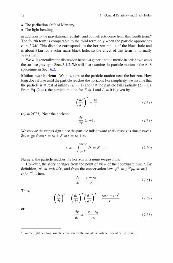
Motion near horizon We now turn to the particle motion near the horizon. Howlong does it take until the particle reaches the horizon? For simplicity, we assume thatthe particle is at rest at infinity (E = 1) and that the particle falls radially (L = 0).From Eq. (2.44), the particle motion for E = 1 and L = 0 is given by
(dr
dτ
)2
= r0r
(2.48)
(r0 = 2GM). Near the horizon,dr
dτ� −1. (2.49)
We choose the minus sign since the particle falls inward (r decreases as time passes).So, to go from r = r0 + R to r = r0 + ε,
τ � −∫ r0+ε
r0+Rdr = R − ε. (2.50)
Namely, the particle reaches the horizon in a finite proper time.However, the story changes from the point of view of the coordinate time t . By
definition, p0 = mdt/dτ , and from the conservation law, p0 = g00 p0 = m(1 −r0/r)−1. Then,
dτ
dt= r − r0
r. (2.51)
Thus, (dr
dt
)2
=(
dr
dτ
)2 (dτ
dt
)2
= r0(r − r0)2
r3(2.52)
ordr
dt� −r − r0
r0(2.53)
4 For the light bending, use the equation for the massless particle instead of Eq. (2.43).

2.3 Physics of the Schwarzschild Black Hole 19
near the horizon, and
t � −r0
∫ r0+ε
r0+R
dr
r − r0= r0(ln R − ln ε), (2.54)
so t → ∞ as ε → 0. Namely, it takes an infinite coordinate time until the particlereaches the horizon. Incidentally, Eq. (2.53) near the horizon takes the same form asthe massless case below. Namely, the particle moves with the speed of light near thehorizon.
Let us consider themassless case. For themassless particle, p2 = 0 or ds2 = 0, so
ds2 = g00dt2 + grr dr2 = 0 (2.55)
→(
dr
dt
)2
= −g00grr
=(1 − r0
r
)2(2.56)
→ dr
dt= −
(1 − r0
r
)� −r − r0
r0. (2.57)
Near the horizon, the expression takes the same form as the massive case (2.53) aspromised. We considered the infalling photon, but one can consider the outgoingphoton. In this case, t → ∞ until the light from the horizon reaches the observer atfinite r .
There is nothing special to the horizon from the point of view of the infallingparticle. But there is a singular behavior from the point of view of the coordinate t .This is because the Schwarzschild coordinates (t, r) are not well-behaved near thehorizon. Thus, we introduce the coordinate systemwhich is easier to see the infallingparticle point of view.
2.4 Kruskal Coordinates
The particlemotion discussed so far can be naturally understood by using a new coor-dinate system, theKruskal coordinates. TheKruskal coordinates (u, v) are defined by
r > r0
⎧⎪⎨⎪⎩
u =(
rr0
− 1)1/2
er/(2r0) cosh(
t2r0
)
v =(
rr0
− 1)1/2
er/(2r0) sinh(
t2r0
) (2.58)
r < r0
⎧⎪⎨⎪⎩
u =(1 − r
r0
)1/2er/(2r0) sinh
(t2r0
)
v =(1 − r
r0
)1/2er/(2r0) cosh
(t2r0
) (2.59)

20 2 General Relativity and Black Holes
Fig. 2.3 Kruskalcoordinates. The light-conesare kept at 45◦, which isconvenient to see the causalstructure. The dashed linerepresents an example of theparticle path. Once theparticle crosses the horizon,it must reach the singularity
r = (constant)
t = (constant)
r = (constant)
r = 0
u
v
r = r 0
t =
By the coordinate transformation, the metric (2.30) becomes
ds2 = 4r30r
e−r/r0(−dv2 + du2) + r2dΩ22 . (2.60)
Here, we use not only (u, v) but also use r , but r should be regarded as r = r(u, v)and is determined by (
r
r0− 1
)er/r0 = u2 − v2. (2.61)
One can see the following various properties from the coordinate transformationand the metric (see also Fig. 2.3):
• The metric (2.60) is not singular at r = r0. There is a singularity at r = 0. Thetransformation (2.58) is singular at r = r0, but this is not a problem. Because thetransformation relates the coordinates which are singular at r = r0 to the coordi-nates which are not singular at r = r0, the transformation should be singular there.
• The null world-line ds2 = 0 is given by dv = ±du. In this coordinate system, thelines at 45◦ give light-cones just like special relativity, which is convenient to seethe causal structure of the spacetime.
• The r = (constant) lines are hyperbolas from Eq. (2.61).• In particular, in the limit r = r0, the hyperbola becomes a null line, so the horizon
r = r0 is a null surface. Namely, the horizon is not really a spatial boundary but isa light-cone. In special relativity, the events inside light-cones cannot influence theevents outside light-cones. Similarly, the events inside the horizon cannot influencethe events outside the horizon. Then, even light cannot reach from r < r0 to r > r0.
• For r < r0, the r = (constant) lines become spacelike. This means that a particlecannot remain at r = (constant) because the geodesics of a particle cannot be

2.4 Kruskal Coordinates 21
spacelike. The singularity at r = 0 is spacelike as well. Namely, the singularity isnot a point in spacetime, but rather it is the end of “time.”
• The t = (constant) lines are straight lines. In particular, the t → ∞ limit is givenby u = v. One can see that it takes an infinite coordinate time to reach the horizon.
To summarize, the particle falling into the horizon cannot escape and necessarilyreaches the singularity.
New keywords
After you read each chapter, try to explain the terms in “New keywords” by yourselfto check your understanding.
horizon cosmological constantproper time Schwarzschild black holeworld-line spacetime singularityfour-velocity gravitational redshiftgeodesic Kruskal coordinatesaffine parameter
Appendix: Review of General Relativity
Consider a coordinate transformation
x ′μ = x ′μ(x). (2.62)
Under a coordinate transformation, a quantity is called a vector if it transforms as
V ′μ = ∂x ′μ
∂xνV ν, (2.63)
and as a 1-form if it transforms “oppositely”:
V ′μ = ∂xν
∂x ′μ Vν . (2.64)
The tensors with a multiple number of indices are defined similarly.In general, the derivative of a tensor such as ∂μV ν does not transform as a tensor,
but the covariant derivative ∇μ of a tensor transforms as a tensor. The covariantderivatives of the vector and the 1-form are given by
∇μV ν = ∂μV ν + V αΓ ναμ , (2.65)
∇μVν = ∂μVν − VαΓ αμν. (2.66)

22 2 General Relativity and Black Holes
As a useful relation, the covariant divergence of a vector is given by
∇μV μ = 1√−g∂μ
(√−gV μ), (2.67)
where g := det g. This can be shown using a formula for a matrix M :
∂μ(det M) = det M tr(M−1∂μM). (2.68)
For example, dxμ transforms as a vector
dx ′μ = ∂x ′μ
∂xνdxν (2.69)
and the metric transforms as
g′μν(x ′) = ∂xρ
∂x ′μ∂xσ
∂x ′ν gρσ (x). (2.70)
Thus, the line element ds2 = gμνdxμdxν is invariant under coordinate transfor-mations. Under the infinitesimal transformation x ′μ = xμ − ξμ(x), Eq. (2.70) isrewritten as
g′μν(x − ξ) = (
δρμ + ∂μξρ
) (δσ
ν + ∂νξσ)
gρσ (2.71)
or
g′μν(x) = gμν(x) + (∂μξρ)gρν + (∂νξ
ρ)gμρ + ξρ∂ρgμν (2.72)
= gμν + ∇μξν + ∇νξμ. (2.73)
In general relativity, an actionmust be a scalar which is invariant under coordinatetransformations. From Eq. (2.69),
d4x ′ =∣∣∣∣∂x ′
∂x
∣∣∣∣ d4x, (2.74)
where |∂x ′/∂x | is the Jacobian of the transformation. On the other hand,√−g
transforms in the opposite manner:
√−g′ =∣∣∣∣ ∂x
∂x ′
∣∣∣∣ √−g. (2.75)
Thus, d4x√−g is the volume element which is invariant under coordinate transfor-
mations.

Appendix: Review of General Relativity 23
The metric is determined by the Einstein-Hilbert action:
S = 1
16πG
∫d4x
√−gR. (2.76)
Here, G is the Newton’s constant, and the Ricci scalar R is defined by the Riemanntensor Rα
μνρ and the Ricci tensor Rμν as follows:
Rαμνρ = ∂νΓ
αμρ − ∂ρΓ α
μν + Γ ασνΓ
σμρ − Γ α
σρΓ σμν, (2.77)
Rμν = Rαμαν, R = gμν Rμν. (2.78)
The variation of the Einstein-Hilbert action gives
δS = 1
16πG
∫d4x
{√−gRμν(δgμν) + (δ√−g)Rμνgμν
+ √−g(δRμν)gμν
}, (2.79)
where gμν is the inverse of gμν . The second term can be rewritten by using5
δ√−g = −1
2
√−ggμνδgμν. (2.80)
One can show that the third term reduces to a surface term, so it does not contributeto the equation of motion.6 Therefore,
δS = 1
16πG
∫d4x
√−g
(Rμν − 1
2gμν R
)δgμν, (2.81)
and by requiring δS = 0, one gets the vacuum Einstein equation:
Rμν − 1
2gμν R = 0. (2.82)
The contraction of Eq. (2.82) gives Rμν = 0.When one adds the matter action Smatter, the equation of motion becomes
Rμν − 1
2gμν R = 8πGTμν, (2.83)
5 Using Eq. (2.68) gives δ(√−g) = 1
2√−ggμνδgμν . Then, use another matrix formula δM =
−Mδ(M−1)M which can be derived from MM−1 = I . Then, δgμν = −gμρ gνσ δgρσ . Note thatδgμν = gμρ gνσ δgρσ . Namely, we do not use the metric to raise and lower indices of the metricvariation.6 Care is necessary to the surface term in order to have a well-defined variational principle. Thisissue will be discussed in Chap.7 App. and Chap.12 App. 1.

24 2 General Relativity and Black Holes
where Tμν is the energy-momentum tensor for matter fields:
Tμν := − 2√−g
δSmatter
δgμν. (2.84)
Various matter fields appear in this book, but the simplest term one can add to theEinstein-Hilbert action is given by
Scc = − 1
8πG
∫d4x
√−gΛ, (2.85)
which is the cosmological constant term. From Eq. (2.84),
Tμν = − Λ
8πGgμν, (2.86)
so the Einstein equation becomes
Rμν − 1
2gμν R + Λgμν = 0. (2.87)

Chapter 3Black Holes and Thermodynamics
Quantummechanically, blackholes have thermodynamic properties just like ordinary statisti-cal systems. In this chapter, we explain the relation between black holes and thermodynamicsusing the example of the Schwarzschild black hole.
3.1 Black Holes and Thermodynamics
For the Schwarzschild black hole, the horizon radius is given by r0 = 2GM/c2. Thehorizon radius is proportional to the black hole mass, so if matter falls in the blackhole, the horizon area increases:
A = 4πr20 = 16πG2M2
c4. (3.1)
Also, classically nothing comes out from the black hole, so the area is a non-decreasing quantity,1 which reminds us of thermodynamic entropy. Thus, one expectsthat a black hole has the notion of entropy S:
S ∝ A? (3.2)
We henceforth call S as the black hole entropy.In fact, a black hole obeys not only the second law but also all thermodynamic-
like laws as we will see (Fig. 3.1). First of all, a stationary black hole has only a fewparameters such as the mass, angular momentum, and charge. This is known as theno-hair theorem (see, e.g., Refs. [1, 2] for reviews). Namely, a black hole does notdepend on the properties of the original stars such as the shape and the composition.
1 As the black hole evaporates by the Hawking radiation, the horizon area decreases. But thetotal entropy of the black hole entropy and the radiation entropy always increases (generalizedsecond law).
© Springer Japan 2015M. Natsuume, AdS/CFT Duality User Guide, Lecture Notes in Physics 903,DOI 10.1007/978-4-431-55441-7_3
25

26 3 Black Holes and Thermodynamics
Fig. 3.1 Comparisonbetween laws ofthermodynamics and blackhole thermodynamics
Thermodynamics Black hole
Zeroth law Temperature T is constant Surface gravity κ is constant
at equilibrium for a stationary solution
First law dE = T dS dM = κ8πG dA
Second law dS ≥ 0 dA ≥ 0
Third law S → 0 as T → 0 S → 0 as T → 0?
Conversely, a black hole is constrained only by a few initial conditions, so thereare many ways to make a black hole. For example, even if the black hole formedfrom gravitational collapse is initially asymmetric, it eventually becomes the simplespherically symmetric Schwarzschild black hole (when the angular momentum andthe charge vanish).
This property of the black hole itself is similar to thermodynamics. Thermody-namics is the theory of many molecules or atoms. According to thermodynamics,one does not have to specify the position and the momentum of each molecule tocharacterize a thermodynamic system. The system can be characterized only by a fewmacroscopic variables such as temperature and pressure. The prescription to go frommicroscopic variables to macroscopic variables is known as the coarse-graining.
The black hole is described only by a few parameters. This suggests that somehowthe black hole is a coarse-grained description. But at present the details of thiscoarse-graining is not clear. This is because we have not completely established themicroscopic theory of the black hole or the quantization of the black hole.
3.1.1 Zeroth Law
Let us compare the black hole laws and thermodynamic laws.2 A thermodynamicsystem eventually reaches a thermal equilibrium, and the temperature becomes con-stant everywhere. This is the zeroth law of thermodynamics. Recall that a black holeeventually becomes the spherically symmetric one even if it is initially asymmetric.Spherical symmetry implies that the gravitational force is constant over the horizon.Then, to rephrase the no-hair theorem, gravity over the horizon eventually becomesconstant even if it was not constant initially. This is similar to the zeroth law, andgravity on the horizon corresponds to the temperature. Also, both temperature andgravity are non-negative. A stationary black hole, whose horizon gravity becomesconstant, is in a sense a state of equilibrium.
The gravitational force (per unitmass) or the gravitational acceleration on the hori-zon is called the surface gravity. In Newtonian gravity, the gravitational accelerationis given by
2 See Sect. 9.2 to refresh your memory of thermodynamics.

3.1 Black Holes and Thermodynamics 27
a = GM
r2, (3.3)
so at the horizon r = r0,
κ = a(r = r0) = c4
4GM. (3.4)
We used Newtonian gravity to derive the surface gravity, but one should not takethe argument too seriously. This is just like the Newtonian gravity result for thehorizon radius in Chap.2. The surface gravity is the force which is necessary tostay at the horizon, but in general relativity, one has to specify who measures it. Asdiscussed below, the surface gravity is the forcemeasured by the asymptotic observer.The infalling observer cannot escape from the horizon, no matter how large the forceis. So, the necessary force diverges for the infalling observer himself. But if this forceis measured by the asymptotic observer, the force remains finite and coincides withthe Newtonian result. Two observers disagree the values of the acceleration becauseof the gravitational redshift.
3.1.2 Surface Gravity �
Consider a generic static metric of the form
ds2 = − f (r)dt2 + dr2
f (r)+ · · · . (3.5)
Here, · · · represents the line element along the horizon which is irrelevant to ourdiscussion. Following Sect. 2.3.2, the particle motion is determined from
(dr
dτ
)2
= E2 − f → d2r
dτ 2= −1
2f ′, (′:= ∂r ). (3.6)
For the Schwarzschild black hole, f = 1 − 2GM/r , so d2r/dτ 2 = −GM/r2. Aswe saw in Sect. 2.3.2, the expression takes the same form as Newtonian gravity.
In this sense, we used Newtonian gravity to derive the particle’s acceleration inthe last subsection. But this acceleration is not the covariant acceleration aμ but isjust the ar component. It is more suitable to use the proper acceleration which is themagnitude of the covariant acceleration3:
a2 := gμνaμaν = f ′2
4 f, (3.7)
3 One can check a0 = 0 for the particle at rest.

28 3 Black Holes and Thermodynamics
a = f ′
2 f 1/2. (3.8)
The proper acceleration diverges at the horizon since f (r0) = 0 at the horizon. Thisis not surprising since the particle cannot escape from the horizon.
The surface gravity is the force (per unit mass) a∞(r0), which is necessary to holdthe particle at the horizon by an asymptotic observer. In order to obtain the force,suppose that the asymptotic observer pulls the particle at r by a massless “string”(Fig. 3.2). If the observer pulls the string by the proper distance δs, the work done isgiven by
W∞ = a∞δs (asymptotic infinity), (3.9)
Wr = aδs (location r). (3.10)
Now, convert the work Wr into radiation with energy Er = Wr at r , and then collectthe radiation at infinity. The energy received at infinity, E∞, gets the gravitationalredshift (Sect. 2.3.1). The redshift formula is Eq. (2.37):
EB
E A=
√g00(A)
g00(B). (3.11)
So, E∞ is given by
E∞ =√
f (r)
f (∞)Er = f (r)1/2aδs, (3.12)
where we used f (∞) = 1. The energy conservation requires W∞ = E∞, so a∞ =f 1/2a = f ′/2 or
κ := a∞(r0) = f ′(r0)2
, (3.13)
which coincides with the naive result (3.6).
particle
“string”
E
W
convert work Wr into radiation Er
r
Fig. 3.2 In order to obtain the surface gravity, the asymptotic observer pulls the particle by amassless “string.” The work done to the particle is then converted into radiation. The radiation issubsequently collected at infinity

3.1 Black Holes and Thermodynamics 29
3.1.3 First Law
If the black hole mass increases by dM, the horizon area increases by dA as well. So,one has a relation
dM ∝ dA. (3.14)
To have a precise equation, compare the dimensions of both sides of the equation.First, the left-hand sidemust beGdM because theNewton’s constant andmass appearonly in the combination GM in general relativity. The Einstein equation tells howthe mass energy curves the spacetime, and G is the dictionary to translate from themass to the spacetime curvature.
Then, one can easily see that the right-hand side must have a coefficient whichhas the dimensions of acceleration. It is natural to use the surface gravity for thisacceleration. In fact, the first law dE = T dS tells us that temperature appears as thecoefficient of the entropy, and we saw earlier that the surface gravity plays the roleof temperature. Thus, we reach
GdM � κdA. (3.15)
By differentiating Eq. (3.1) with respect to M , one can see that
GdM = κ
8πdA (3.16)
including the numerical constant. This is the first law of black holes.We discuss the third law of black holes in Sect. 3.3.3.
3.2 From Analogy to Real Thermodynamics
3.2.1 Hawking Radiation
We have seen that black hole laws are similar to thermodynamic laws. However, sofar this is just an analogy. The same expressions do not mean that they representthe same physics. Indeed, there are several problems to identify black hole laws asthermodynamic laws:
1. Nothing comes out from a black hole. If the black hole really has the notion oftemperature, a black hole should have a thermal radiation.
2. The horizon area and the entropy behave similarly, but they have different dimen-sions. In the unit kB = 1, thermodynamic entropy is dimensionless whereas thearea has dimensions. One can make it dimensionless by dividing the area bylength squared, but so far we have not encountered an appropriate one.

30 3 Black Holes and Thermodynamics
The black hole is not an isolated object in our universe. For example, mattercan make a black hole, and the matter obeys quantum mechanics microscopically.So, consider the quantum effect of matter. If one considers this effect, the blackhole indeed emits the black body radiation known as the Hawking radiation, and itstemperature is given by
kBT = �κ
2πc(3.17)
= �c3
8πGM, (Schwarzschild black hole). (3.18)
This is a quantum effect because the temperature is proportional to �. We explainlater how to derive this temperature, the Hawking temperature. Anyway, once thetemperature is determined, we can get the precise relation between the black holeentropy S and the horizon area A. The first law of black hole (3.16) can be rewritten as
d(Mc2) = κc2
8πGdA (3.19)
= �κ
2πkBc
kBc3
4G�dA = T
kBc3
4G�dA. (3.20)
So, comparing with the first law of thermodynamics dE = TdS, one obtains
S = A
4G�kBc3 = 1
4
A
l2plkB . (3.21)
Here, lpl = √G�/c3 ≈ 10−35 m is called the Planck length. The Planck length is the
length scale where quantum gravity effects become important. Note that one cannotmake a quantity whose dimension is the length from the fundamental constants ofclassical mechanics alone, G and c. The black hole entropy now becomes dimen-sionless because we divide the area by the Planck length squared. Equation (3.21) iscalled the area law.
A few remarks are in order. First of all, our discussion here does not “derive”S as the real entropy. Microscopically, the entropy is the measure of the degreesof freedom of a system, but we have not counted microscopic states. We are stillassuming that classical black hole laws are really thermodynamic laws.
Second,
• The black hole entropy is proportional to the “area.”• On the other hand, the statistical entropy is proportional to the “volume” of asystem.

3.2 From Analogy to Real Thermodynamics 31
This difference is extremely important for AdS/CFT and gives a clue on the natureof microscopic states of black holes. Because these entropies behave differently,a four-dimensional black hole cannot correspond to a four-dimensional statisticalsystem. But the five-dimensional “area” is the four-dimensional “volume.” Then, afive-dimensional black hole can correspond to a four-dimensional statistical system.Namely,
First clue of AdS/CFT:The black hole entropy suggests that a black hole can be described bythe usual statistical system whose spatial dimension is one dimensionlower than the gravitational theory.
AdS/CFT claims that this statistical system is a gauge theory. Such an idea is calledthe holographic principle in general [3, 4]. The holographic principle is the first cluefor AdS/CFT, and we will see another clue, the large-Nc gauge theory, in Sect. 4.2.
Now, our discussion so far uses the Schwarzschild black hole as an example,but the formula (3.21) itself is generic. The black hole entropy is always given byEq. (3.21) as long as the gravitational action iswritten by the Einstein-Hilbert action4:
1
16πGd
∫dd x
√−gR. (3.22)
Namely, Eq. (3.21) is true not only for black holes in general relativity but also forblack holes in string theory and in the other gravitational theories.
3.2.2 Hawking Temperature and Euclidean Formalism
There are several ways to compute the Hawking temperature. Hawking originallycomputed it by quantizing matter fields in the black hole background. But the simpleway is to require that the Euclidean spacetime be smooth. To do so, one needs aperiodic identification in imaginary time, and the temperature is the inverse of thisperiod β.
By the analytic continuation to Euclidean signature tE = it, the metric (3.5)becomes
ds2E = + f (r)dt2E + dr2
f (r)+ · · · . (3.23)
4 For a generic gravitational action, the black hole entropy is given by the Wald formula [5].

32 3 Black Holes and Thermodynamics
Let us focus on the region near the “horizon” r � r0. Near the horizon, f (r0) = 0,so one can approximate5 f � f ′(r0)(r − r0). Then,
ds2E � dr2
f ′(r0)(r − r0)+ f ′(r0)(r − r0)dt2E (3.24)
= dρ2 + ρ2d
(f ′(r0)2
tE
)2
, (3.25)
where we introduced a new coordinate ρ := 2√
(r − r0)/ f ′(r0). In this coordinate,the metric takes the same form as a plane in polar coordinates if f ′(r0)tE/2 has theperiod 2π . Otherwise, the metric has a conical singularity at ρ = 0. The periodicityof tE is given by β = 4π/ f ′(r0) or
T = f ′(r0)4π
. (3.26)
If one compares this result with Eq. (3.13), one gets T = κ/(2π)which is Eq. (3.17).For the Schwarzschild black hole, f (r) = 1 − r0/r , so
T = 1
4πr0= 1
8πGM. (3.27)
Note that the Euclidean metric does not cover inside the horizon r < r0 since thehorizon is the origin of polar coordinates.
What is behind the Euclidean formalism is quantum statistical mechanics. Inquantum statistical mechanics, the periodicity in the imaginary time is naturallyassociated with the inverse temperature. We mimic this technique of quantum sta-tistical mechanics and apply to black holes. Then, the “first-principle” computationof black hole thermodynamic quantities is carried out as follows [6]. (This approachnaturally leads to the GKP-Witten relation in AdS/CFT later.)
The problem of quantum gravity is not completely solved, but it is natural toexpect that quantum gravity is defined by a path integral such as
Z =∫
Dg eiSL[g]. (3.28)
Here, SL is the gravitational action, and the above equation shows the path integralover the metric g schematically. We consider the Euclidean formalism with tE = it,SE = −iSL:
Z =∫
Dg e−SE[g]. (3.29)
5 Here, we assume f ′(r0) = 0. This assumption fails for extreme black holes where two horizonsare degenerate (Sect. 3.3.3).

3.2 From Analogy to Real Thermodynamics 33
As we saw above, the Euclidean black hole is periodic in time. Then, it is natural toassociate the statistical mechanical partition function to the black hole and is naturalto regard Z as such a partition function. However, it is not clear how to carry out thepath integral because it diverges.Also, string theorydoes not evaluateEq. (3.29) itself.In any case, whether one uses string theory or uses the above approach, semiclassicalresults themselves should agree. Semiclassically, the most dominant contribution tothe path integral comes from an extremum of the action, or the classical solution(saddle-point approximation). Under the approximation,
Z � e−SE . (3.30)
Here,SE is the on-shell action which is obtained by substituting the classical solutionto the action. The free energy F is then given by SE = βF . For example, for theSchwarzschild black hole, one can show that
F = r04G
= 1
16πGT. (3.31)
Then, one can get thermodynamic quantities:
S = −∂T F = 1
16πGT 2 = πr20G
= A
4G, (3.32)
E = F + T S = 1
8πGT= r0
2G= M. (3.33)
We will not carry out the actual computation for the Schwarzschild black holehere but will carry out for the Schwarzschild-AdS5 black holes in Chap.7 App. andSect. 14.2. AdS/CFT identifies the black hole partition function Z as the gauge theorypartition function.
3.2.3 On the Origin of Black Hole Entropy �
What represents the black hole entropy? It is not easy to answer to the question aswe will see below, but let us make some general remarks.
When we are speaking of the entropy of the sun, the meaning is clear. Althougha thermodynamic system looks same macroscopically, the system can have differentmicroscopic states. There are number of ways one can distribute, e.g., a given energyto amultiple number of particles. The entropy counts the number of possible quantumstates when macroscopic variables such as energy are specified. In general, thisnumber becomes larger when the number of particles becomes larger. So, the entropyis generically proportional to the number of particles.

34 3 Black Holes and Thermodynamics
This suggests that the black hole entropy counts the microscopic states a blackhole can have. This number can be estimated as follows [7]. Let us imagine to makea black hole by collecting particles in a small region. The entropy is proportional tothe number of particles. To have a larger entropy, we let the total number of particlesas many as possible, or we make the black hole from light particles. However, theCompton wavelength of a particle with mass m is about λ � �/m. We cannot collectparticles in a smaller region than the Compton wavelength. But to make a blackhole, we must collect them within the Schwarzschild radius. Thus, if the Comptonwavelength is larger than the Schwarzschild radius, a black hole is not formed.Consequently, we cannot choose the particle mass freely, and the lightest particle wecan use has mass which satisfies �/m � 2GM. Then, the total number of particlesis given by
Nmax � M
m� M
�
2GM
� (GM)2
G�� A
G�, (3.34)
which is the right order-of-magnitude for the black hole entropy.This is fine for a rough estimate, but how can one derive the black hole entropy
statistical mechanically? The Planck length lpl appears in the denominator of the arealaw (3.21). This means that the microscopic derivation of the black hole entropy islikely to require quantumgravity. But the formulation of quantumgravity is a difficultproblem, so the problem of the black hole entropy is not completely resolved. Stringtheory is the prime candidate of the unified theory including quantum gravity, andstring theory can derive the black hole entropy microscopically for some black holes(see, e.g., Refs. [8, 9] for reviews).
In Sect. 3.2.2, we briefly discussed the semiclassical computation of the blackhole entropy. It is natural that such a computation gives the black hole entropy andis not just a coincidence. There should be something behind which justifies thecomputation. But one can say that it is not satisfactory as the microscopic derivationof the black hole entropy, namely as the statistical derivation of the black hole entropy:
• First, Eq. (3.29) itself is not well-defined and cannot be estimated beyond thesemiclassical approximation.
• Also, the computation does not tell us what degrees of freedom the black holeentropy corresponds to.
But AdS/CFT gives an interesting interpretation to the semiclassical result.AdS/CFT identifies the partition function computed in this way as the partitionfunction of a gauge theory. AdS/CFT claims the equivalence between two theo-ries, a gauge theory and a gravitational theory, and there are two points of view onecan take:
• Namely, one can use the gravitational theory to know about the gauge theory.• Or, one can use the gauge theory to know about the gravitational theory.
Because AdS/CFT claims the equivalence, it is hard to say which point of view ismore fundamental, namely which theory is more fundamental, but let us take thelatter point of view for now. If so, one can regard the origin of the black hole entropy

3.2 From Analogy to Real Thermodynamics 35
as the entropy of the corresponding gauge theory, namely the number of microscopicstates of the gauge theory. Then, the black hole entropy is nothing but the usualstatistical entropy.
However, black holes in AdS/CFT are the ones in AdS spacetime. It is not clearif one can make such an interpretation for any black holes, in particular for theSchwarzschild black hole. The holographic principle seems to suggest that this issomehow possible.
3.3 Other Black Holes
3.3.1 Higher-Dimensional Schwarzschild Black Holes
The four-dimensional Schwarzschild black hole can be generalized to d-dimensionalspacetime:
ds2d = − f (r)dt2 + dr2
f (r)+ r2dΩ2
d−2, (3.35)
f (r) = 1 −(r0
r
)d−3 = 1 − 16πGd
(d − 2)Ωd−2
M
rd−3 , (3.36)
Ωn = 2πn+12
Γ( n+1
2
) . (3.37)
Here, Gd is the Newton’s constant in d-dimensional spacetime, dΩ2n is the line
element of the unit Sn (see Sect. 6.1.5 for an explicit construction), andΩn is its areawhich is written by the Gamma function Γ (n +1/2). Some explicit forms of Ωn aregiven by
Ω0 = 2, Ω1 = 2π, Ω2 = 4π, Ω3 = 2π2,
Ω4 = 8
3π2, Ω5 = π3, Ω6 = 16
15π3, Ω7 = 1
3π4. . . .
(3.38)
The behavior 1/rd−3 in f (r) comes from the fact that the Newtonian potentialbehaves as 1/rd−3 in d-dimensional spacetime.
Using Eqs. (3.21) and (3.26), one gets thermodynamic quantities:
T = f ′(r0)4π
= d − 3
4πr0, (3.39)
S = A
4Gd= rd−2
0 Ωd−2
4Gd. (3.40)
One can check the first law with these quantities and the mass (3.36).

36 3 Black Holes and Thermodynamics
3.3.2 Black Branes
The black holes in previous subsection are simply the extensions of the four-dimensional black hole, but in higher dimensions, there exist black holes which donot appear in four-dimensions. The Schwarzschild black hole has a spherical hori-zon, but the horizon can take other topologies in higher dimensions.6 In particular,the horizon can have an infinite extension.
A simple example is the five-dimensional “neutral black string,” which is thefour-dimensional Schwarzschild black hole times R:
ds25 = −(1 − r0
r
)dt2 + dr2
1 − r0r
+ r2dΩ22 + dz2, (3.41)
where z represents the R coordinate. For the five-dimensional Schwarzschild blackhole, the horizon, the r = r0 surface has the line element r20dΩ2
3 which representsthe S3-horizon. Here, the horizon is still given by r = r0, but the horizon has theline element r20dΩ2
2 + dz2. So, the horizon has the topology S2 × R and extendsindefinitely in z-direction. Such a horizon is called a planar horizon. When we saythe word “black hole” in this book, it is mostly a black hole with a planar horizon.A black hole with planar horizon is often called a black brane.
The black branes arise with various dimensionalities. A black brane with Rp
horizon is called a black p-brane. Namely,
p = 0 black holep = 1 black stringp = 2 black membrane
......
To obtain thermodynamic quantities of the neutral black string, notice that the blackstring is just the four-dimensional Schwarzschild black hole if one compactifies thez-direction. Then, the black string and the four-dimensional Schwarzschild blackhole have the same thermodynamic quantities. Take the periodicity of z as V1. Bythe compactification,
1
16πG5
∫d5x
√−g5R5 = V1
16πG5
∫d4x
√−g4 (R4 + · · · ) , (3.42)
where the dots denote matter fields which appear by the compactification. Thus,the four-dimensional Newton’s constant G4 is written as 1/G4 = V1/G5 from thefive-dimensional point of view. Then, thermodynamic quantities are
6 For four-dimensional asymptotically flat black holes, the topology of black hole horizons must beS2 under appropriate conditions on matter fields. This is known as the topology theorem (see, e.g.,Proposition 9.3.2 of Ref. [10]) which is part of the no-hair theorem.

3.3 Other Black Holes 37
Fig. 3.3 Gregory-Laflammeinstability
V1
Black String
Black Hole
r0
~r0
?
T = 1
4πr0, S = πr20
G4= πr20
G5V1, M = r0
2G4= r0
2G5V1, P = − r0
4G5,
(3.43)
where we used the first law dM = TdS − PdV1 to derive the pressure P . The entropyof the black string is rewritten as
Sstring = 4πG5M2
V1. (3.44)
Gregory-Laflamme instability � Asa side remark, the neutral black string actuallyhas the so-called Gregory-Laflamme instability [11] (see, e.g., Refs. [12, 13] forreviews). The black string is not the only neutral solution allowed, but the five-dimensional Schwarzschild black hole is also allowed. Even though the z-directionis compactified, the metric (3.35) should be good approximately when the horizonradius r0 satisfies r0 V1. The thermodynamic quantities behave as
M � r20G5
, SBH5 � r30G5
� √G5M3/2. (3.45)
On the other hand, the entropy of the black string behaves as Eq. (3.44). Considerthe microcanonical ensemble with fixed M . Then, SBH5 > Sstring for a large enoughV1, so the black hole is favorable entropically. Then, the black string is unstable andwould decay to the black hole, but it is still not clear if the transition really occurs(Fig. 3.3). Anyway, it has been shown numerically that the neutral black string isunstable under perturbations.7
7 It has been argued that the Gregory-Laflamme instability is related to the Rayleigh-Plateau insta-bility in hydrodynamics [14].

38 3 Black Holes and Thermodynamics
3.3.3 Charged Black Holes
A black hole can have a charge Q. The solution is known as the Reissner-Nordströmblack hole (RN black hole hereafter):
ds2 = −(1 − 2GM
r+ GQ2
r2
)dt2 + dr2
1 − 2GMr + GQ2
r2
+ r2dΩ22 (3.46)
= −(1 − r+
r
) (1 − r−
r
)dt2 + dr2(
1 − r+r
) (1 − r−
r
) + r2dΩ22 , (3.47)
Fr0 = Q
r2, (3.48)
where 2GM = r+ + r− and GQ2 = r+r−. We chose the dimensions of Q asdimensionless. (The charge is dimensionless in the units c = � = 1.)
The RN black hole is a solution of the Einstein-Maxwell theory8:
S =∫
d4x√−g
(1
16πGR − 1
16πF2
). (3.49)
The equations of motion from the above action is given by
Rμν − 1
2gμν R = 2G
(Fμρ F ρ
ν − 1
4gμν F2
), (3.50)
∇ν Fμν = 0. (3.51)
Here, we check only the Maxwell equation:
∇ν Fμν = 1√−g∂ν(
√−gFμν) = 0. (3.52)
When a black hole has an electric charge, Fr0 = Er = 0, and the only nontrivialequation is ∂r (
√−gFr0) = 0. For the above metric, Fr0 = −Fr0 and√−g =
r2 sin2 θ , so the solution to the Maxwell equation is given by Eq. (3.48). The fieldstrength Fμν is written by the gauge potential Aμ as Fμν = ∂μ Aν − ∂ν Aμ. For ourelectric field, one may choose the gauge potential A0 as
A0 = − Q
r. (3.53)
The black hole (3.47) has two horizons r = r±, where
r± = GM ±√
G2M2 − GQ2. (3.54)
8 Note the normalization of the Maxwell action. This choice is standard for the RN black hole.

3.3 Other Black Holes 39
But note that
• When√
GM > Q, two horizons exist.• When
√GM < Q, there is no horizon since Eq. (3.54) becomes complex.
• The limiting case√
GM = Q or r+ = r− is called the extreme black hole.
Also, the black hole has a spacetime singularity at r = 0.
Thermodynamic quantities Again using Eqs. (3.21) and (3.26), one gets
T = r+ − r−4πr2+
= 1
2π
√G2M2 − GQ2
2GM(
GM +√
G2M2 − GQ2)
− GQ2, (3.55)
S = 4πr2+4G
= π
G
(GM +
√G2M2 − GQ2
)2
. (3.56)
The black holes with√
G M > Q emit the Hawking radiation and eventually settleinto the extreme black hole. The extreme black hole has zero temperature.9
When a thermodynamic system exchanges particle numbers or charges with theenvironment, the first law becomes
dM = T dS + μdQ, (3.57)
where μ is the “chemical potential.” This is just the gauge potential A0 in this case.However, the value of A0 itself is not meaningful due to the gauge invariance:
A0(x) → A0(x) + ∂0Λ(x). (3.58)
What is physical is the difference of the gauge potential.Imagine to add a charge ΔQ from the asymptotic infinity to the black hole. This
requires energy ΔE proportional to the difference of A0 between the asymptoticinfinity and the horizon (for a same sign charge as the black hole). Then, μ shouldbe given by
μ = A0|r=∞ − A0|r=r+ , (3.59)
9 Since the Hawking temperature is proportional to the surface gravity, a zero temperature blackhole has zero surface gravity. Then, does the black hole have no gravitational force? As we sawpreviously, the surface gravity is the gravitational force measured by the asymptotic observer. Butthe asymptotic observer and the observer near the horizon disagree the value of the force because ofthe gravitational redshift. Although there is a gravitational force for the observer near the horizon,it vanishes for the asymptotic observer.

40 3 Black Holes and Thermodynamics
and ΔE = μΔQ which takes the form of the first law. Thus,
μ = Q
r+=
√1
G
r−r+
. (3.60)
Using these thermodynamic quantities, one can show the first law (3.57).10
Third law According to the third law of thermodynamics, S → 0 as T → 0 (Nernst-Planck postulate). On the other hand, the entropy of the RN black hole remains finiteas
√G M → Q, so the black hole seems to violate the third law.
This point is still controversial, but a finite entropy at zero temperature means thatground states are degenerate, and there is nothing wrong about degenerate groundstates quantum mechanically. However, such a degeneracy is often true only in ide-alized situations, and the degeneracy is normally lifted by various perturbations.Similarly, the degeneracy of the RN black hole may be lifted by various interactions.
3.4 Summary
• A black hole behaves as a thermodynamic system and has thermodynamic quan-tities such as energy (mass), entropy, and temperature.
• The black hole entropy is proportional to the horizon area. This suggests that ablack hole can be described by the usual statistical systemwhose spatial dimensionis one dimension lower than the gravitational theory (holographic principle).
• To derive black hole thermodynamic quantities, use the Euclidean path integralformulation and evaluate the path integral by the saddle-point approximation.
• These are various black objects (black branes) in higher dimensions.
New keywords
black hole thermodynamics holographic principleblack hole entropy Euclidean formalismno-hair theorem planar horizonsurface gravity black braneHawking temperature Reissner-Nordström black holePlanck length extreme black holearea law
10 On the other hand, for the RN black hole (and for the Schwarzschild black hole), the otherthermodynamic relations such as the Euler relation and the Gibbs-Duhem relation do not takestandard forms (see App.).

Appendix: Black Holes and Thermodynamic Relations � 41
Appendix: Black Holes and Thermodynamic Relations �
We saw that black holes satisfy the first law. The first law should be always satisfiedbecause the law simply represents the energy conservation. On the other hand, theother thermodynamic relations such as the Euler relation and the Gibbs-Duhemrelation do not take standard forms for black holes with compact horizon. The storyis different for black branes though: these relations take standard forms like standardthermodynamic systems.
For example, thermodynamic quantities of the Schwarzschild black hole aregiven by
T = 1
4πr0, S = πr20
G4, E = r0
2G4. (3.61)
So, the Euler relation does not take the form E = TS, but
E = 2TS, (3.62)
which is known as the Smarr’s formula.For black holes with compact horizon, thermodynamic relations do not take stan-
dard forms because these black holes do not satisfy fundamental postulates of ther-modynamics (Sect. 9.2). In particular, thermodynamics requires that the entropy isadditive over the subsystems. This requirement is unlikely to hold in the presenceof a long-range force such as gravity. Another related problem is that the volume Vand its conjugate quantity, pressure P , do not appear in those black holes (at least asindependent variables.)
The postulate in particular implies that the so-called fundamental relation of astandard thermodynamic system
S = S(E, V ) (3.63)
is a homogeneous first order function of extensive variables:
S(λE, λV ) = λS(E, V ). (3.64)
Then, the Euler relation and the Gibbs-Duhem relation follow from the fundamentalrelation. However, if one rewrites Eq. (3.61) in the form of the fundamental relation,one gets
SBH4 = 4πG4E2, (3.65)
which is a homogeneous second order function in E . Thus, it is no wonder thatthermodynamic relations do not take standard forms.
However, the story is different for branes. For branes, one has an additional exten-sive variable, volume V , and the entropy is additive over the subsystems along thebrane direction V = VA + VB . In this sense, the entropy of branes is additive, and

42 3 Black Holes and Thermodynamics
branes satisfy the standard postulates of thermodynamics. A simple example is theneutral black string (3.41). In Eq. (3.44), we wrote the entropy of the black string inthe form of the fundamental relation:
Sstring = 4πG5E2
V1. (3.66)
This is indeed a homogeneous first order function in extensive variables. As a result,one can check that the black string does satisfy the standard thermodynamic relationsE = TS − PV1 and SdT − V1dP = 0. Note that Eqs. (3.65) and (3.66) are actuallythe same equation since V1/G5 = 1/G4.
References
1. J.D. Bekenstein, Black hole hair: 25-years after. arXiv:gr-qc/96050592. M. Heusler, No hair theorems and black holes with hair. Helv. Phys. Acta 69, 501 (1996).
arXiv:gr-qc/96100193. G. ’t Hooft, Dimensional reduction in quantum gravity. arXiv:gr-qc/93100264. L. Susskind, The world as a hologram. J. Math. Phys. 36, 6377 (1995). arXiv:hep-th/94090895. R.M. Wald, Quantum Field Theory in Curved Space-time and Black Hole Thermodynamics
(The University of Chicago Press, Chicago, 1994)6. G.W. Gibbons, S.W. Hawking, Action integrals and partition functions in quantum gravity.
Phys. Rev. D15, 2752 (1977)7. W.H. Zurek, K.S. Thorne, Statistical mechanical origin of the entropy of a rotating, charged
black hole. Phys. Rev. Lett. 54, 2171 (1985)8. G.T. Horowitz, The origin of black hole entropy in string theory. arXiv:gr-qc/96040519. A. Dabholkar, S. Nampuri, Quantum black holes. Lect. Notes Phys. 851, 165 (2012).
arXiv:1208.4814 [hep-th]10. S.W. Hawking, G.F.R. Ellis, The Large Scale Structure of Spacetime (Cambridge University
Press, Cambridge, 1973)11. R. Gregory, R. Laflamme, Black strings and p-branes are unstable. Phys. Rev. Lett. 70, 2837
(1993). arXiv:hep-th/930105212. G.Horowitz (ed.),Black Holes in Higher Dimensions (CambridgeUniversityPress,Cambridge,
2012)13. T. Harmark, V. Niarchos, N.A. Obers, Instabilities of black strings and branes. Class. Quantum
Gravity 24, R1 (2007). arXiv:hep-th/070102214. V. Cardoso, O.J.C. Dias, Rayleigh-Plateau andGregory-Laflamme instabilities of black strings.
Phys. Rev. Lett. 96, 181601 (2006). arXiv:hep-th/0602017

Chapter 4Strong Interaction and Gauge Theories
So far we discussed black holes, but this chapter describes another important element ofAdS/CFT, gauge theory. After we overview the theory of strong interaction, namely QCD,its phase structure, and heavy-ion experiments, we explain the idea of the large-Nc gaugetheory. This idea naturally leads us to AdS/CFT.
4.1 Strong Interaction and QCD
4.1.1 Overview of QCD
Protons and neutrons are made out of more fundamental particles, quarks. Undernormal circumstances, quarks are bound together inside protons and neutrons, andone cannot liberate them. The strong interaction is the force which bounds quarkstogether. The theory of the strong interaction is described by quantum chromody-namics, or QCD. QED is a gauge theory based on U (1) gauge symmetry, and QCDis based on SU (3) gauge symmetry. The strong interaction is meditated by gluons,which are the SU (3) gauge fields.
A quark belongs to the fundamental representation of SU (3) and can take 3 states.These degrees of freedom are called color; this is the origin of the word ‘chromo’in quantum chromodynamics. If we denote the color degrees of freedom by indexi , a quark can be written as qi (i = 1, 2, 3).1 An antiquark qi has an anticolor. Forthe electromagnetic interaction, an electric charge is the source of the interaction;similarly, for the strong interaction, a “color charge” is the source of the interaction.
A quark has a color, but the quark color typically changes by a quark-gluoninteraction. The difference of color is carried off by the gluon. Thus, the gluoncarries one color and one anticolor. A gluon behaves as a quark-antiquark pair2 qi q j .
1 Quarks have the additional degrees of freedom, flavor. There are 6 flavors, up u, down d, stranges, charm c, bottom b, and top t .2 This does not mean that a gluon is a quark-antiquark pair. It simply means that a gluon transformslike a quark-antiquark pair under SU (3).
© Springer Japan 2015M. Natsuume, AdS/CFT Duality User Guide, Lecture Notes in Physics 903,DOI 10.1007/978-4-431-55441-7_4
43

44 4 Strong Interaction and Gauge Theories
Then, using a 3× 3 matrix on index (i, j), one can write a gluon as (Aμ)ij . Namely,
a gluon belongs to the adjoint representation of SU (3).A gluon, the force carrier itself has color charges, so a gluon has the self-
interactions. This point is very different from QED; the force carrier of the elec-tromagnetic force, photon, is electrically neutral. This aspect changes the dynamicsof QCD from QED drastically.
TheQCD interaction becomes weak at high energy (asymptotic freedom), and onecan rely on the perturbative QCD. This was helpful to confirm QCD as the theory ofstrong interaction since the predictions from the perturbative QCD can be comparedwith the results from the deep inelastic scattering experiments. On the other hand, theQCD interaction becomes stronger at low energy. Because of this property, quarksand gluons are confined into particles collectively known as hadrons, and only the“color-neutral” particles appear.3 This is known as the color confinement, but thishas not been proven yet.
QCD has the invariance under the quark phase transformation q → eiθq. This isthe global U (1)B symmetry associated with the baryon number conservation.
4.1.2 Phase Structure of QCD
QCD becomes strongly-coupled at low energy, and one cannot rely on the pertur-bation theory. But this situation suggests that QCD has rich phenomena, richer thanQED. In fact, QCD has a rich phase structure, and the full details of the phase struc-ture are still unclear (Fig. 4.1).4 The region “χSB” in this figure is the phase wherequarks are confined.
At high temperature, many light particles are excited, and the interaction betweenquarks is screened by light particles in between. This is the Debye screening, aphenomenon which also occurs in QED.5 The quark-gluon plasma, or QGP, is thephase where quarks and gluons are deconfined by the screening.6
Just like the usual electromagnetic plasma, QGP is made of “charged ionized”particles in a sense. The differences lie in the meaning of the “charge” and “ioniza-tion.” For QGP, we mean color charges, not electric charges. The quarks of coursecarry electric charges as well, but it is not important here. Also, what we meantby ionization is the deconfinement for QGP. The transition to QGP is estimated asTc ≈ 150 − 200MeV ≈ 1 fm ≈ 2 × 10¹² K. However, according to lattice simula-tions, this is not a sharp phase transition but a smooth “cross-over” at zero baryon
3 Strictly speaking, one should say that only color singlets appear.4 Such a rich phase structure is not limited to QCD and is common to Yang-Mills gauge theories.The large-Nc gauge theories seem to have a rich phase structure in general as we will see gradually.5 What is screened in QCD is not electric charge but color charges. As a result, the strong interactionbecomes weak.6 See Ref. [2] for the textbook in QGP.

4.1 Strong Interaction and QCD 45
T
Fig. 4.1 QCD phase diagram [1]. The vertical axis represents temperature, and the horizontal axisrepresents the so-called “baryon chemical potential,” which is associated with the baryon numberconservation (see footnote 10 in Sect. 9.2 for the use of the terminology chemical potential). In thefigure, “χSB” (which stands for chiral symmetry breaking) represents the hadron phase, and “CSC”represents the so-called color superconducting phase. This is just a schematic diagram, and the fulldetails of the phase diagram are still unclear; at this moment, it is not clear if there are any otherphases in this diagram, and the boundaries of each phases are not clear either
chemical potential. (In Fig. 4.1, the solid line which represents the phase boundarydoes not cross the vertical axis, which means the cross-over.)
Naively, one would expect that the perturbation theory is valid in the plasma phasesince the deconfinement occurs there. It is true that the plasma should behave likea free gas at high enough temperatures. But the strong interaction does not becomeweak enough at the temperatures one can realize in current experiments. This isbecause the QCD coupling constant decreases only logarithmically with energy,1/ log E . In fact, there is an experimental indication that QCD is still strongly-coupled in the plasma phase (Sect. 4.1.4). But then, even if one would like to discussplasma properties theoretically, one cannot rely on the perturbative QCD. We needanother approach to study QGP.
The lattice simulation is a useful approach at strong coupling, which becomesvery powerful in recent years. But this approach is the imaginary-time formalismnot the real-time formalism. As a consequence, this is very powerful for equilibriumproblems but is not powerful yet for nonequilibrium problemswhich are the situationat QGP experiments. Also, currently the analysis at finite density is difficult as well.
4.1.3 Heavy-Ion Experiments
The quark-gluon plasma is a natural phenomenon from QCD. In fact, theoretically ithas been known for a long time. But it was never formed in an experiment, let alone

46 4 Strong Interaction and Gauge Theories
tomeasure physical properties. But in recent years, there exist heavy-ion experimentswhose goals are to form QGP and to measure its physical properties.
Particle accelerators usually collide e+e−, pp or p p, but the heavy-ion experi-ments collide heavy nuclei such as gold nuclei. Heavy atoms themselves are elec-trically neutral. In order to accelerate them, one has to strip electrons and to ionizethem. So, such an experiment is called a heavy-ion experiment.
One notable heavy-ion accelerator is the Relativistic Heavy Ion Collider (RHIC),which is located at Brookhaven National Laboratory and is in operation since 2000.Another heavy-ion experiment has been performed at CERN since 2010 using theLarge Hadron Collider (LHC). The plasma temperature by these colliders are esti-mated as about 2Tc at RHIC and about 5Tc at LHC.
In heavy-ion experiments, one first collides heavy nuclei, and the plasma is formedif the temperature is high enough. But the plasma exists only transiently; the hightemperature of the plasma causes it to expand, and then the plasma cools down bythe expansion. In the end, the temperature is below the transition temperature, soquarks are confined into hadrons. What is observed is these secondary particles. Theabove history shows the difficulties of the experiment and its analysis:
• The plasma has a very complicated time-evolution so that its analysis is not easy.• What is observed is not QGP itself but only its by-products such as hadrons. Onehas to infer what happened from the by-products. Thus, it is not an easy job toconfirm even the QGP formation.
• Many secondary particles are involved in the experiments. The purpose here is theQGP property as a thermal system, so one has to keep track of these particles asmany as possible.
• Finally, the perturbative QCD is not very effective for theoretical analysis as dis-cussed below.
4.1.4 “Unexpected Connection Between String Theoryand RHIC Collisions”
In 2005, the first detailed RHIC results were announced at the APS annual meeting.This press release has an interesting statement [3]: “The possibility of a connectionbetween string theory and RHIC collisions is unexpected and exhilarating.”7 (Direc-tor of the DOE Office of Science) Here, “string theory” meant the AdS/CFT duality.What is the “unexpected connection” between string theory and RHIC collisions?
In the RHIC announcement, it was stressed that quark-gluon-plasma does notbehave like a free gas but behaves more like a perfect fluid.8 The difference between
7 As far as I know, this is the first time string theory has been mentioned in the announcement of amajor experiment.8 Actually, the announcement stated that QGP behaves like a perfect “liquid” to avoid the technicalterm “fluid,” but it was slightly misleading. See footnote 9 for more details.

4.1 Strong Interaction and QCD 47
Fig. 4.2 Left When onemoves the upper plate, thefluid is dragged due to theviscosity and the lower plateexperiences a force. Rightthe close-up view of the fluid
v
L
F
x
a free gas and a perfect fluid is that the latter has no viscosity. We will discuss theviscosity and hydrodynamics in Chap.9 in details, but let us remind you of freshmanphysics of viscosity.
As a simple example, consider a fluid between two plates and move the upperplate with velocity v (Fig. 4.2). As the fluid is dragged, the lower plate experiences aforce. This force is the manifestation of the viscosity. In this case, the force the lowerplate experiences per unit area F /A is given by
F
A= η
v
L. (4.1)
The proportionality constant η is called the shear viscosity.Microscopically, the viscosity arises due to themomentum transfer betweenmole-
cules. Figure4.2 (right) shows a close-up view of the fluid and we put an artificialboundary to divide the fluid into two parts. The molecules collide with each otherand are exchanged randomly through the boundary. But in the situation where wemove the upper plate, the molecules in the upper-half part, on average, have moremomentum in the x-direction than the ones in the lower-half part. These moleculesare exchanged,whichmeans thatmomentum in the x-direction is transported throughthe boundary. This is the microscopic origin of the viscosity.
The shear viscosity has units of [η] = Pa · s = kg ·m−1 · s−1 from Eq. (4.1). Thus,one would expect from dimensional analysis that the shear viscosity is given by
η � ρvlmfp � ετmfp (4.2)
(ρ:mass density, v:mean velocity of particles, lmfp:mean-free path, ε: energy density,τmfp: mean-free time). Now, change the coupling constant. At strong coupling, the

48 4 Strong Interaction and Gauge Theories
mean-free path becomes shorter. The viscosity arises due to the momentum transfer,and the transfer is less effective at strong coupling. So, the viscosity becomes smallerat strong coupling. In particular, a perfect fluid has no viscosity, so a perfect fluid is astrong coupling limit. This is somewhat confusing, but an ideal gas is the free limit,and a perfect fluid is the strong coupling limit.9
A small viscosity implies the strong interaction. According to RHIC, QGP has asmall viscosity, so this implies that QGP is strongly-coupled. This is an interestingdiscovery, but then how can one study such a strong coupling problem theoretically?One cannot rely on the perturbative QCD. This is one main obstacles in the QGPresearch. String theory may be a good place to study such an issue. It turns outthat the prediction of the shear viscosity using AdS/CFT is close to the RHIC result(Chap. 12). This is the “unexpected connection” the RHIC announcement meant.
We will further discuss heavy-ion experiments and their results in Sect. 12.2.
4.2 Large-Nc Gauge Theory
In QCD, the perturbation theory has a limited power, and it is still difficult to solveQCD nonperturbatively. An approximation method, the so-called large-Nc gaugetheory, was proposed by ’t Hooft, and this idea is naturally related to string theory[5].10
There are three colors in QCD, but in the large-Nc gauge theory, one considersa large number of colors. For example, consider a U (Nc) gauge theory. The gaugefield is written as an Nc × Nc matrix, (Aμ)i
j .Then, the theory has two parameters,
gauge theory coupling constant gYM, number of colors Nc.
Instead, we will use Nc and the ’t Hooft coupling λ := g2YMNc as independent
parameters. The large-Nc limit is given by11
Nc → ∞ while λ is kept fixed and large.
9 The argument here has some limitations. First, the fluidmust be aNewtonian fluid. [TheNewtonianfluids are the fluids which satisfy Eq. (4.1).] Second, among Newtonian fluids, we consider onlythe fluids where the momentum transfer occurs due to the mechanism described in the text. Forexample, “honey” satisfies neither of these conditions.
This is an appropriate place to go back to the RHIC announcement of “perfect liquid.” In ourdiscussion, the fluid is always gas-like and the momentum transfer is kinematic (i.e., the momentumis transferred by particle motion), whereas in a liquid, the momentum transfer by potential energyamong particles is more effective (see, e.g., Ref. [4]). What we have in mind is the strong couplinglimit of the QGP gas. In this sense, saying that QGP is a perfect liquid is slightly misleading. Butin the strong coupling limit, the distinction between a gas and a liquid becomes rather subtle.10 See Chap.8 of Ref. [6] for the details of the large-Nc gauge theory.11 If one recovers gYM, the limit implies gYM → 0.

4.2 Large-Nc Gauge Theory 49
Fig. 4.3 The propagator ofthe gauge field (wavy lines)and the interaction vertex bydouble-line notations (top,middle). The bottom figure isan example of vacuumamplitudes
This is a nontrivial limit as we will see. Namely, the theory does not reduce to thefree one in this limit because the effective coupling is given by λ. Thus, λ � 1 is astrong coupling limit.
The large-N limit of, e.g., O(N ) vector model often appears in condensed-matterphysics. The large-Nc gauge theory has the same spirit but has important differences.The vector model is solvable in this limit, but the gauge theory is hard to solve evenin this limit. Also, the vector model essentially reduces to a classical theory. Thegauge theory also reduces to a classical theory, but this classical theory is a classicalgravitational theory as we will see in a moment.
In Feynman diagrams, a gauge theory propagator is represented by a single line.But to keep track of colors, it is convenient to use the “double-line notation,” wherethe propagator is represented by a double-line with opposite arrows (Fig. 4.3). Then,draw diagrams so that the direction of arrows is preserved. As far as color indices areconcerned, the gauge field behaves as a quark-antiquark pair, so one can regard thedouble-line as the pair. Namely, one line represents the rows of the matrix (Aμ)i
j ,and the other represents the columns.
Or, in string theory context, a double-line represents the propagation of an openstring because an open string represents a gauge field (Chap. 5). A double-line cor-responds to the endpoints of a string.12
The Lagrangian of a gauge field is schematically written as
L = 1
g2YM
{∂ A∂ A + A2∂ A + A4} = Nc
λ{· · · }. (4.3)
12 We will encounter string theory again in the large-Nc limit below, but this string is not the sameas the open string here. String theory appeared below is a closed string theory.

50 4 Strong Interaction and Gauge Theories
(a) (b) (c)
Fig. 4.4 Examples of vacuum amplitudes. Figure a and b are planar diagrams, and c is a non-planardiagram
From the Lagrangian, one can derive Feynman rules to obtain amplitudes. Here isthe summary of rules:
• Associate the factor λ/Nc for each propagator.• Associate the factor Nc/λ for each interaction vertex.13
• Associate the factor Nc for each loop (because of the summation over Nc colors).
Denote the number of vertices as V , the number of propagators as E , and the numberof loops as F . From the Feynman rules, one gets
(Nc
λ
)V (λ
Nc
)E
N Fc = λE−V N V −E+F
c . (4.4)
For example, the diagram4.4a has (V, E, F) = (2, 3, 3), so
(Nc
λ
)2 (λ
Nc
)3
N 3c = λN 2
c . (4.5)
The diagram4.4b has (V, E, F) = (4, 6, 4), so
(Nc
λ
)4 (λ
Nc
)6
N 4c = λ2N 2
c . (4.6)
Thus, these results are summarized schematically as
(1 + λ + λ2 + · · · )N 2c = f0(λ)N 2
c . (4.7)
But it is not always the case that diagrams take the form (4.7). For example, thediagram4.4c has (V, E, F) = (4, 6, 2), so
13 In Fig. 4.4, the vertex is represented by a gray dot. Below we will take care only of the factorsNc and λ in diagrams, and we will discuss only “vacuum amplitudes” with no external lines.

4.2 Large-Nc Gauge Theory 51
Fig. 4.5 Relation between a diagram and a two-dimensional surface
(Nc
λ
)4 (λ
Nc
)6
N 2c = λ2. (4.8)
The diagrams such as Fig. 4.4a, b are called planar, and the diagrams such as Fig. 4.4care called non-planar. Theword “planar” (“non-planar”)means that one can (cannot)draw the diagrams on a plane. Including non-planar diagrams, the diagrams arewritten as
f0(λ)N 2c + f1(λ)N 0
c + f2(λ)1
N 2c
+ · · · . (4.9)
In the large-Nc limit, the first term of Eq. (4.9), the planar diagrams, dominate.Whether diagrams dominate in the large-Nc limit depends on whether one can
draw them on a plane (or a sphere). This strongly suggests the relation between thediagrams and topology. In fact, one can draw the diagram4.4c on a torus.14
In general, one can understand the relation between these diagrams and topologyin the followingway. Let us fill in loopswith surfaces.One can construct a closed two-dimensional surface (Fig. 4.5). Each propagator is an edge of the surface (polygon),and each vertex is a vertex of the polygon. Then, one can regard the number ofpropagators E as the number of edges, and the number of loops F as the number offaces of the polygons. Now, in this interpretation, the power of Nc in Eq. (4.4) is theEuler characteristic χ , which is a topological invariant:
χ = V − E + F. (4.10)
For example, a sphere has χ = 2, and a torus has χ = 0. If we denote the number ofhandles (genus) as h, one can alsowriteχ = 2−2h. Namely, the planar diagram4.4a,b correspond to the sphere, and the non-planar diagram4.4c corresponds to the torus(Fig. 4.6).
14 This is beyond my ability to draw such an illustration. Anyway, such an illustration is hard tosee. I recommend readers to draw such an illustration on their own or to draw diagrams on an objectwith a handle (such as a doughnut or a mug).

52 4 Strong Interaction and Gauge Theories
Fig. 4.6 Diagrams andtopology
Now, the summation of vacuum diagrams is a partition function, so the partitionfunction is given by
ln Zgauge =∞∑
h=0
Nχc fh(λ) (4.11)
or
Second clue of AdS/CFT:The partition function of a large-Nc theory is given bya summation over the topologies of two-dimensional surfaces.
As one can see fromFig. 4.4a, b, themore propagatorswe have, themore dominanta diagram is in the large-Nc limit. This limit is hard to evaluate in a field theory. Onthe other hand, the two-dimensional surface point of view becomes better in thislimit. The diagrams become denser in this limit, and they approach a smoother two-dimensional surface.
In the next chapter, we will see that the perturbative expansion of string theory isalso given by a summation over two-dimensional topologies (Fig. 5.12). This “coin-cidence” leads one to guess that two theories, gauge theory and string theory, areactually equivalent:
Zgauge = Zstring. (4.12)
In particular, a summation of two-dimensional closed surfaces corresponds to thegravitational perturbative expansion. There, the sphere, the planar diagrams, corre-sponds to classical gravity, and the torus, one of non-planar diagrams, correspondsto gravity at one-loop. In Sect. 3.2.1, the holographic principle gives the first clue forAdS/CFT, and the large-Nc gauge theory gives us the second clue.
4.3 Summary 53
4.3 Summary
• According to heavy-ion experiments, QGP behaves as a perfect fluid with a verysmall shear viscosity. This implies that QGP is strongly-coupled.
• It is difficult to compute gauge theories such as QCD at strong coupling. Thelarge-Nc gauge theory provides an approximation to compute a strong couplinglimit.
• The partition function of a large-Nc theory is given by a summation over thetopologies of two-dimensional surfaces.
New keywords
quarks quark-gluon plasma (QGP)quantum chromodynamics (QCD) heavy-ion experimentsgluons perfect fluidfundamental/adjoint representation shear viscositycolor ’t Hooft couplingflavor large-Nc limitasymptotic freedom double-line notationhadrons planar/non-planarcolor confinement topologyDebye screening
References
1. T. Hatsuda, Bulk and spectral observables in lattice QCD. arXiv:hep-ph/07022932. K. Yagi, T. Hatsuda, Y.Miake,Quark-Gluon Plasma: From Big Bang To Little Bang (Cambridge
University Press, Cambridge, 2005)3. http://www.bnl.gov/newsroom/news.php?a=13034. L.P. Csernai, J.I. Kapusta, L.D. McLerran, On the strongly-interacting low-viscosity matter cre-
ated in relativistic nuclear collisions. Phys. Rev. Lett. 97, 152303 (2006). arXiv:nucl-th/06040325. G. ’t Hooft, A planar diagram theory for strong interactions. Nucl. Phys. B72, 461 (1974)6. S. Coleman, Aspects of Symmetry (Cambridge University Press, Cambridge, 1985)

Chapter 5The Road to AdS/CFT
In this chapter, we explain basics of string theory and howone reachesAdS/CFT. The relationbetween string theory and gauge theory has been discussed for many years, and AdS/CFTsolved the “homework” to some extent.
We should give a warning about this chapter. The discussion in this chapter needsstring theory to some extent, which may be frustrating to readers. So, we choose toexplain string theory intuitively, but, on the other hand, our argument here is not veryrigorous. Anyway, readers do not have to worry about string theory part much ifyou just want to know the AdS/CFT technique. This is because we rarely use stringtheory itself in actual AdS/CFT computations. Nevertheless, we include the materialbecause
1. AdS/CFT makes a bold claim that a four-dimensional gauge theory is equivalentto a five-dimensional gravitational theory: two theories look different, and eventheir spacetime dimensions are different. The road to AdS/CFT gives us someother clues why this can be true.
2. String theory was originally born as the theory of strong interaction. But thereweremanyproblems for the approach at that time. Following the path toAdS/CFT,one can understand how AdS/CFT circumvented these problems.
5.1 String Theory: Prehistory
The strong interaction is described by QCD, but string theory was originally born asthe theory of strong interaction before QCD.
For example, a meson is a quark-antiquark pair, and it is explained well by the“string” which connects the pair (Fig. 5.1). The string has the tension. In order toseparate the pair, one needs energy proportional to the string length R, E ∝ R,so quarks cannot be separated, which explains the confinement. In reality, when thestring length becomes large enough, the potential energy is large enough to create anew quark-antiquark pair. Then, a string breaks into two strings. But the endpointsof strings are still quarks and antiquarks, and one cannot get individual quarks inisolation.
© Springer Japan 2015M. Natsuume, AdS/CFT Duality User Guide, Lecture Notes in Physics 903,DOI 10.1007/978-4-431-55441-7_5
55

56 5 The Road to AdS/CFT
Fig. 5.1 The string model ofa meson
quark antiquark
tension
string
Because the string has the tension T, it would collapse to a point. In order thestring not to collapse, one needs to oscillate the string. Or if the string rotates, thestring becomes stable by balancing the tension and the centrifugal force. But theangular momentum J (or the oscillation) of the string contributes to the energy Mof the string, so there is a relation between J and M .
Such a relation can be obtained from the dimensional analysis. We consider therelativistic string and use the unit c = 1. In this unit, [J ] = ML and [T] = ML−1.(Recall J = r × p. The mass density has the same dimensions as T in these units.)Classically, such a string has only the tension T as the dimensionful parameter [see,e.g., Eq. (8.34)]. Thus, we must have
J � 1
TM2 + � . (5.1)
Here, we added the second term which is a quantum correction.Indeed, the meson spectrum satisfies such a relation. Phenomenologically, the
relation (5.1) is fitted by two parameters α′ and α(0):
J = α′M2 + α(0) . (5.2)
From the above discussion, 1/α′ represents the tension, and α(0) represents thequantum correction. (Note that in the units c = � = 1, [α′] = L2 and α(0) isdimensionless.) This relation is known as a Regge trajectory. Figure5.2 is the Reggetrajectory for typical mesons.1
The pions are the most well-known among all mesons. They are made of u and dquarks as well as their antiquarks. The ρ mesons are also made of them. Althoughthe pions have spin 0 (scalar meson), the ρ mesons have spin 1 (vector meson) andheavier mass. Now, there is a series of mesons which are similar to the ρ mesons buthave larger spins and heavier masses. These mesons lie on a single line with2
α′ ≈ 0.9GeV−2, α(0) ≈ 0.5. (5.3)
The mesons are explained by the string model well. Of course, eventually QCDappeared as the theory of strong interaction, but the string model is not inconsis-tent with QCD. The flux lines of electrodynamics spread in space. However, color
1 Such a figure is known as a Chew-Frautschi plot [2].2 To be precise, this line does not represent a single trajectory but represents degenerate trajectorieswhich are distinguished by the other quantum numbers. Incidentally, the ω mesons contain ss, butthey are similar to the ρ mesons in the sense that they do not carry quantum numbers such asstrangeness, charm, bottom, and top.

5.1 String Theory: Prehistory 57
Fig. 5.2 An example ofRegge trajectories. Thehorizontal axis representsM2, and the vertical axisrepresents spins. The mesonsin square brackets are notwell-known. The straightline is fitted using Eq. (5.3).Reproduced with permissionfrom Ref. [1]
0
1
2
3
4
5
6
0 1 2 3 4 5 6 7 8
Fig. 5.3 The QCD flux linesform a thin flux tube (right)unlike the electromagneticflux lines (left)
flux lines do not spread but rather form a thin flux tube because gluons have self-interactions (Fig. 5.3). It is natural to imagine that mesons are well-described by thestring model when the thickness of the flux tube is negligible.
Thus, string theory has nice properties as a theory of strong interaction, but thereare shortcomings as well. In particular,
Problem 1: In order to quantize the string consistently, one needs a higher dimen-sional spacetime. The bosonic string, which contains only bosons in thespectrum, requires 26-dimensional spacetime, and string theory whichalso contains fermions requires 10-dimensional spacetime. Otherwise,the theory is not consistent.
Problem 2: One can describe the confinement as a string connecting quarks, butwhat appears in QCD is not only the confining potential. When thequark separation becomes smaller, the thickness of the flux tube is nolonger negligible, and the flux lines look more like the usual one. Asa consequence, one has the Coulomb-like potential, E ∝ −1/R. Thesimple stringmodel is unlikely to describe this effect. Also, in the plasmaphase, one has the Debye screening by thermally excited light quarks.From the string model point of view, the string becomes easier to breakby quark pairs, but this implies that the string description is not veryadequate. In a nutshell, the string model looks like a model of confine-ment only. If string theory really describes QCD, one should be able todiscuss the full phase diagram of QCD.
We will reexamine Problem 1 in Sect. 5.3 and Problem 2 in Sect. 8.2.

58 5 The Road to AdS/CFT
These problems suggest that something is clearly missing about the corre-spondence between the strong interaction and string theory. Moreover, QCD wasproposed, and QCD was proved to be the right theory of the strong interaction asexperimental results accumulated. So, string theory as the strong interaction wasonce abandoned. Rather, string theory was reincarnated as the unified theory includ-ing gravity. We will then quickly look at this aspect of string.
5.2 String Theory as the Unified Theory
Figure5.4 shows the contents of the standardmodel. There are 6 quarks and 6 leptonsas matters and 4 forces act on matters. In principle, all phenomena can be understoodwith these elements, but the standard model has many shortcomings as well. We willnot describe these shortcomings, but in brief, the problem is that the standard modelis a disjointed framework.
This is particularly clear in the force sector. Gravity is described by general rela-tivity and this is a classical theory. On the other hand, the other 3 forces are describedby gauge theories, and gauge theories can be quantized. So, theoretical foundationsand concepts for these forces are completely different. Now, string theory is thetheory which unifies all these elements.
5.2.1 String Oscillations and Elementary Particles
The fundamental object in string theory is the very small string (Fig. 5.5). There aretwo kinds of string: open stringswith endpoints and closed stringswith no endpoints.The string has only the tension T as the dimensionful parameter. Since [T] = L−2,we introduce a parameter ls with the dimension of length.3 The parameter ls is calledthe string length and represents the characteristic length scale of the string. The stringlength ls is the only fundamental length scale in string theory. The string length isabout 10−34 m. But currently the length we can see experimentally is about 10−17 m.So, macroscopically the string is just a point particle.
But no matter how small the string is, there is a big difference between strings andpoint particles; namely, a string can oscillate and a string can oscillate in variousways.This is the advantage of the string. There are many kinds of elementary particles inparticle physics. String theory unifies all particles in nature as different oscillationsof string.
3 The parameters T, α′, and ls are related by
T = 1
2πα′ = 1
2πl2s. (5.4)

5.2 String Theory as the Unified Theory 59
6 kinds of leptonsMatter 6 kinds of quarks
Forces gravity general relativity (classical theory)electromagnetic forceweak forcestrong force
gauge theories (quantum theories)
Higgs boson
Fig. 5.4 The standard model of elementary particles
Fig. 5.5 Main ingredients of string theory. An open string with endpoints and a closed stringwithout endpoints
Fig. 5.6 The simplest oscillations of an open string. The initial configurations in thick curvesbecome gray curves after the half period. The “box” here is drawn to see the oscillations easier
Let us look at string oscillations closely. Figure5.6 shows the simplest open stringoscillation (in four dimensions). As one can see, the string can oscillate in twodirections. So, the open string has two degrees of freedom at this level. These degreesof freedom represent two polarizations of a gauge field (photon). In this sense, theopen string represents a gauge theory.4
On the other hand, a closed string represents a graviton. Again, the easiest way tosee this is to look at how the string oscillates (Fig. 5.7). In general, the oscillationson a string have two modes: the left-moving mode and right-moving mode. Foran open string, these modes mix each other at endpoints, but these modes becomeindependent for a closed string. So, one can oscillate the right-moving mode in onedirection and the left-moving mode in the other direction. In a sense, a closed string
4 Classically, such a string oscillation represents a massive particle as one can expect from Eq. (5.2).But it is actually massless because of the quantum correction [the second term of Eq. (5.2)]. This istrue only in 26-dimensional spacetime for the bosonic string and in 10-dimensional spacetime forsuperstrings. This is one reason why higher-dimensional spacetime is necessary in string theory.

60 5 The Road to AdS/CFT
Fig. 5.7 A closed string has two independent modes, which corresponds to the spin-2 nature of thegraviton
oscillates in two directions simultaneously. This property explains the spin-2 natureof the graviton. In fact, a graviton also oscillates in two directions simultaneously.5
5.2.2 D-brane
An open string propagates through spacetime just like a closed string, but an openstring can also have its endpoints on an object, the so-called D-brane (Fig. 5.8a)[3, 4]. Although these open strings are constrained to have their endpoints on theD-brane, these are open strings, so they still describe gauge theories. But because theendpoints are constrained on the D-brane, the gauge theory described by the D-braneis localized on the D-brane.
If there are Nc coincident D-branes, open strings can have endpoints in variousways. Open strings can have endpoints on the same brane or can have endpoints onthe different branes (two curved lines and one straight line in Fig. 5.8b). These newdegrees of freedom correspond to SU (Nc) degrees of freedom.6
TheD-branes arisewith various dimensionalities.AD-branewith a p-dimensionalspatial extension is called the Dp-brane. Namely,
p = 0 point-like objectp = 1 string-like objectp = 2 membrane-like object
......
5 More precisely, the simplest oscillations of a closed string represents a graviton and two undis-covered scalar particles, the dilaton and the axion. Since left and right-moving modes each have twodegrees of freedom, a closed string has four degrees of freedom at this level (in four dimensions).The graviton has only two degrees of freedom, and two scalar fields cover the remaining degreesof freedom.6 More precisely, the D-branes represent a U (Nc) gauge theory, but the U (1) part describes thecenter of mass motion of the branes and decouple from the SU (Nc) part.

5.2 String Theory as the Unified Theory 61
(a) (b)
Fig. 5.8 a An open string can have endpoints on aD-brane. bThe Nc coincident D-branes representa SU (Nc) gauge theory. In the figure, the branes are separated for illustration, but we consider thecoincident branes in reality
Thus, the Dp-brane describes a (p +1)-dimensional gauge theory. We are interestedin four-dimensional gauge theories, so consider the D3-brane in order to mimicQCD.7
The D-branes are related to the black branes in Sect. 3.3.2. Some of black branesare gravitational descriptions of D-branes.
In App. 2, we discuss more about the D-brane, the gauge theory that the D3-branerepresents, and its role in AdS/CFT.
5.2.3 Why Open and Closed Strings?
In string theory, there are two kinds of strings, the open string and the closed string.Why are there two kinds of strings? Or one would say that string theory is not aunified theory since there are two kinds of strings. But actually these are the sameobject in a sense. To see this, let us consider how strings interact with each other.
Figure5.9 is the simplest interaction for open strings. Two open strings join intoone open string. But if the endpoints of two open strings can join, the endpointsof a single open string can join as well. Otherwise, one has to require a nonlocalconstraint on the string dynamics. Thus, the endpoints of a single open string canjoin to produce a closed string. Namely, if there are open strings, one has to haveclosed strings. This is the reason why we have two kinds of strings.8
Because an open string represents a gauge theory and a closed string representsgravity, string theory must contain both gauge theory and gravity. This is the uniquefeature of string theory as the unified theory.
The AdS/CFT duality utilizes this unique feature. The AdS/CFT duality relatesa gauge theory to a gravitational theory. This is possible only for the unified theorysuch as string theory. In conventional field theory, a gauge theory and a gravitationaltheory are completely separated since theoretical foundations and concepts are very
7 This is not necessarily the case if one compactifies part of brane directions (e.g., Sakai-Sugimotomodel [5]). Incidentally, theD1-brane is a string-like object, but it is different from the “fundamentalstring” we have discussed so far.8 One can consider string theories with closed string alone, but we will not discuss such theories.

62 5 The Road to AdS/CFT
Fig. 5.9 Top the simplest interaction for open strings is the joining of two strings into one. Bottomif the endpoints of two open strings can join, the endpoints of a single open string can join as well
different. As a result, there is no way to get a relation between a gauge theory and agravitational theory.
There is a bigger picture behind AdS/CFT. Namely, AdS/CFT requires the exis-tence of a unified theory behind.
5.2.4 String Interactions
A particle draws a world-line in spacetime. Similarly, a string sweeps a two-dimensional surface, a world-sheet, in spacetime. In Fig. 5.10a, we draw a Feynmandiagram for a particle, which represents an interaction vertex. For a closed string,such an interaction is replaced by Fig. 5.10b.
In order to express the strength of the interaction, we assign the string couplingconstant gs for an emission/absorption of a closed string. A closed string 1-loop(Fig. 5.11) has an emission and an absorption of a virtual closed string, so it isproportional to g2
s . Figure5.11 has one “handle”, so we can rephrase the rule toassign g2
s for each handle. If we have one more loop, we have one more handle, sothe diagram has the factor g4
s .To summarize, string interactions are classified by the world-sheet topologies
(Fig. 5.12).9 If we denote the number of handles (genus) as h, a h-loop has the factorg2h
s . The genus h is related to the Euler characteristic χ by χ = 2− 2h, and vacuumamplitudes can be written as 1/gχ
s using the Euler characteristic.10
The open string case is similar. Assign the open string coupling constant gs foran emission of an open string. Then, the open string interactions are classified by thetopologies of world-sheets with holes (Fig. 5.13). However, the open string naturallyaccompanies the closed string as we saw earlier, and open string interactions are
9 Below we often consider only vacuum amplitudes for simplicity, but one can consider scatteringamplitudes by adding appropriate external lines. Incidentally, gs looks like a free parameter of thetheory at this stage, but actually it is not a free parameter (Sect. 5.2.5).10 If one adds three external lines (factor g3
s ) to the sphere 1/g2s , the diagram is proportional to gs ,
which is consistent with the interaction vertex in Fig. 5.10b.

5.2 String Theory as the Unified Theory 63
Fig. 5.10 a A Feynmandiagram which represents aninteraction vertex. b Thecorresponding interaction forclosed strings
~ gs
(a) (b)
Fig. 5.11 A 1-loop of closedstrings
~ gs2
Fig. 5.12 The perturbativeexpansion of string theory isgiven by the sum over thetopologies of world-sheetsurfaces
gs21gs2
Fig. 5.13 a An open stringinteraction. b A 1-loop ofopen strings
~ gs~~ gs2~
(a) (b)
Fig. 5.14 An open string1-loop can be viewed as anemission of a closed string

64 5 The Road to AdS/CFT
related to closed string interactions. In fact, an open string 1-loop can be viewed asan emission of a closed string (Fig. 5.14), so we obtain
gs � g2s . (5.5)
5.2.5 Supergravity: Classical Gravity Approximationof String Theory
Wehave seen that the simplest oscillations of strings correspond to gauge theories andgravity. But a string has an infinite number of harmonics, so string theory predictsan infinite number of elementary particles. Since string oscillations cost energy,these infinite number of harmonics correspond to massive particles whose massesare determined by energy of oscillations. This mass is typically O(1/ ls), which isextremely heavy as elementary particles. Thus, what normally matters is a set of thelowest oscillations only; they correspond to known particles.
String theory describes a finite number of known particles when one can ignorethe string length ls , so string theory should be written by standard field theories.Moreover, when gs � 1, only the lowest order of topology expansion, tree diagrams,dominates. In such a case, classical field theories should be enough to describe stringtheory. Such a theory is known as supergravity.11
The form of supergravity action can be determined from general principles.12 Forexample, one can show that string theory graviton has general covariance, so thegravity part should be given by
S = 1
16πG10
∫d10x
√−gR (5.6)
just like general relativity. We write it as a 10-dimensional action since superstringtheory can be quantized consistently only in 10-dimensional spacetime. G10 is theNewton’s constant in 10-dimensional spacetime. Similarly, one can show that gaugefields in string theory have gauge invariance, so the gauge theory part should be givenby the usual gauge theory action.
In string theory, the fundamental coupling constant is the string coupling constantgs . In supergravity, coupling constants are G10 and the gauge field coupling constantgYM. Then, one can relate gs to supergravity coupling constants. By expandinggμν = ημν + hμν , the graviton action is schematically written as
S = 1
16πG10
∫d10x {∂h∂h + h∂h∂h + h2∂h∂h + · · · }. (5.7)
11 See Ref. [6] for a textbook of supergravity. The name, supergravity, comes from the fact that thetheory has local supersymmetry, but we will not discuss the terms with fermions below.12 More properly, one calculates string Feynman diagrams as in Sect. 5.2.4 and writes down a fieldtheory action which reproduces these scattering amplitudes.

5.2 String Theory as the Unified Theory 65
This implies that a graviton emission is proportional to G1/210 . Since a closed string
emission is proportional to gs , one gets G10 ∝ g2s .
Similarly, the gauge field action is schematically written as13
S = 1
g2YM
∫d p+1x {∂ A∂ A + A2∂ A + A4}. (5.8)
This implies that a gauge field emission is proportional to gYM. Since an open stringemission is proportional to gs � g1/2
s ,
g2YM ∝ gs . (5.9)
The dimensional analysis further constrains the form of field theory couplingconstants. Since we usually take the metric as dimensionless, the Newton’s constanthas dimensions [G10] = L8 from Eq. (5.7). In string theory, the fundamental stringscale is only the string length ls which represents the characteristic length scale ofthe string. Thus, G10 � g2
s l8s . Similarly, the gauge field has dimensions [A] = L−1
from Eq. (5.8). In order for the action to be dimensionless, [g2YM] = Lp−3. Thus,
g2YM � gsl p−3
s . To summarize,
G10 � g2s l8s , g2
YM � gsl p−3s . (5.10)
The action (5.6) is the approximation when one can ignore the string length ls .When the string length can no longer be ignored, the action has an infinite numberof terms with powers of curvature tensors such as
S = 1
16πG10
∫d10x
√−g (R + l2s R2 + · · · ). (5.11)
Such corrections are known as α′-corrections.14 From the field theory point of view,these terms correspond to higher derivative terms in an effective field theory,15 andthey originated from integrating out massive fields with mass O(1/ ls). Roughlyspeaking, these terms can be ignored when l2s R � 1, or the length scale of thecurvature is much larger than the string length.
In the topology expansion of string theory, these terms correspond to the lowestorder diagrams, the sphere. Note that the classical gravity approximation of stringtheory corresponds to Eq. (5.11), not Eq. (5.6). However, one often considers the casewhere the spacetime curvature is small. In such a case, the action (5.6) is enough, orthe action (5.11) with the lowest α′-corrections is enough.
13 We write the (p + 1)-dimensional action instead of a 10-dimensional action because one canconsider (p + 1)-dimensional gauge theories using D-branes.14 Recall that the parameter α′ is related to the string length ls by α′ = l2s .15 See Ref. [7] for a review of effective field theories.

66 5 The Road to AdS/CFT
Finally, to be more precise, supergravity typically takes the form
S = 1
16πG10
∫d10x
√−g e−2φ{
R + 4(∇φ)2}
+ · · · (5.12)
instead of the action (5.6). Here, φ is a scalar field called the dilaton. One charac-teristic feature of Eq. (5.12) is that the Ricci scalar part does not take the simpleEinstein-Hilbert form but has the dilaton factor e−2φ . This means that the Newton’sconstant or the string coupling constant actually correspond to the constant part ofthe dilaton e−2φ0 . Readers do not have to worry this fact much since the dilaton isconstant in the simplest AdS/CFT (the D3-brane case in the language of D-branes inSect. 5.2.2). But the dilaton may have a nontrivial behavior in a generic AdS/CFT.A nontrivial dilaton means that the Newton’s constant is not really a constant but itcan vary. Similarly, the gauge field coupling constants can vary because the gaugetheory actions can have a dilaton factor.
5.3 Reexamine String Theory as the Theory of StrongInteraction
5.3.1 Comparison of Partition Functions
We have seen in Sect. 4.2 that the vacuum amplitudes of large-Nc gauge theoriesare given by a summation over the topologies of two-dimensional surfaces. Thisstructure is the same as the closed string amplitudes in Sect. 5.2.4. Since the closedstring represents gravity, the closed string expansion corresponds to the gravitationalperturbative expansion. In particular, the sphere corresponds to classical gravity, andthe torus corresponds to gravity at 1-loop.
This implies that a large-Nc gauge theory is represented by string theory andin particular is represented by classical gravitational theory of string theory in thelarge-Nc limit. This is an amazing conclusion. The original theory is a gauge theorywhich does not include gravity, but it is represented by a gravitational theory in thespecial limit. In this way, the relation between the gauge theory and string theory,which was once abandoned (Sect. 5.1), again emerges.
More explicitly, we saw in Sect. 4.2 that the gauge theory partition function Zgaugeis given by
ln Zgauge =∞∑
h=0
Nχc fh(λ). (5.13)

5.3 Reexamine String Theory as the Theory of Strong Interaction 67
On the other hand, from the discussion in this chapter, the string theory partitionfunction Zstring is given by
ln Zstring =∞∑
h=0
(1
gs
)χ
fh(ls). (5.14)
Since string theory has α′-corrections, We write the dependence as fh(ls). Equa-tions (5.13) and (5.14) have the same structure, so we arrive at the relation
Zgauge = Zstring, (5.15)
and the parameters between two theories are related by16
N 2c ∝ 1
g2s
∝ 1
G, λ ↔ ls, (5.16)
where we also used the relation G ∝ g2s .
The analysis of large-Nc gauge theories leads us to string theory as the theory ofstrong interaction. However, as we mentioned before, one needs higher-dimensionalspacetime in order to quantize string theory consistently. If one assumes the d-dimensional Poincaré invariance17 ISO(1, d − 1), d = 26 for the bosonic stringwhich contains only bosons in the spectrum, and d = 10 for string theory whichalso contains fermions in the spectrum. String theory in four-dimensional spacetimeis not consistent. Namely,
• According to gauge theories, a large-Nc gauge theory is represented by a stringtheory.
• On the other hand, string theory is not valid as a four-dimensional theory.
These two statements sound inconsistent.These two statements are actually not inconsistent. To realize this, one should
recall that string theory is a theory with gravity as well. Namely, string theory shouldadmit not only the flat spacetime as the solution but also curved spacetimes as thesolutions. Onemay use such a curved spacetime to represent a large-Nc gauge theory.The curved spacetime itself can be a higher-dimensional one. The resulting theorycan be interpreted as a flat four-dimensional theory if the curved spacetime has onlythe ISO(1, 3) invariance instead of ISO(1, d − 1). For this purpose, the spacetimedimensionality must be at least five-dimensions, and the fifth direction is curved.
The appearance of the five-dimensional curved spacetime is also natural from theblack hole entropy. A five-dimensional black hole has entropy which is proportionalto the five-dimensional “area.” But an “area” in five dimensions is a “volume” in
16 The parameters Nc and λ are dimensionless whereas G and ls are dimensionful, but we makethe dimensions to come out right in Sect. 5.3.3.17 The Poincaré invariance is also called the inhomogeneous Lorentz invariance. ISO(1, 3) =R1,3 × SO(1, 3).

68 5 The Road to AdS/CFT
four dimensions: This is appropriate as the entropy of a four-dimensional statisticalsystem.
To summarize,18
A large-Nc gauge theory is represented by a five-dimensional curvedspacetime with four-dimensional Poincaré invariance ISO(1, 3).
Such a metric is written as19
ds25 = Ω(w)2(−dt2 + dx23) + dw2. (5.18)
Here, xμ = (t, x3) = (t, x, y, z). The metric contains the combination −dt2 + dx23,
so it has the ISO(1, 3) invariance on (t, x3). Thus, x3-directions correspond to thespatial directions of the large-Nc gauge theory.
Hereafter, Greek indices μ, ν, . . . run though 0, . . . , 3 and are used for the four-
dimensional “boundary” spacetime where a gauge theory lives. On the other hand,capital Latin indices M, N , . . . are used for the five-dimensional “bulk” spacetimewhere a gravitational theory lives.
5.3.2 Scale Invariance and Its Consequences
Without further information, we cannot go any further into the relation between thelarge-Nc gauge theory and the curved spacetime. First, it is not clear what kind ofgauge theory is represented by the curved spacetime. Namely, it is not clear if sucha gauge theory is close to QCD or is the one which behaves differently from QCD.Second, it is not clear what kind of curved spacetime is represented by the gaugetheory. One cannot determine the factor Ω(w). We will impose one more conditionto identify both the gauge theory and the curved spacetime. As we argue below, theappropriate condition is the scale invariance.
Scale invariant gauge theory (classical) When a theory has no scale or no dimen-sionful parameter, it is natural to expect that physics does not change under the scaletransformation:
xμ → axμ. (5.19)
18 I am not aware of who first made this claim explicitly, but see, e.g., Refs. [8, 9] for early attempts.19 The factor Ω does not depend on (t, x3) because of the translational invariance on (t, x3).Incidentally, one can consider the metric of the form
ds25 = Ω1(w′)2(−dt2 + dx2
3) + Ω2(w′)2dw′2, (5.17)
but the metric reduces to Eq. (5.18) by redefining w′.

5.3 Reexamine String Theory as the Theory of Strong Interaction 69
The (classical) scale invariance is an important property of four-dimensional puregauge theories. For example, consider the Maxwell theory:
S = − 1
4e2
∫d4x Fμν Fμν. (5.20)
The action has no dimensionful parameter and is invariant under the scaling with
Aμ → 1
aAμ. (5.21)
If a field Φ transforms asΦ → a−ΔΦ, (5.22)
under the scaling (5.19), we call that the field has scaling dimension20 Δ. TheMaxwell field has scaling dimension 1. Roughly speaking, the scaling dimensioncoincides with the mass dimension (the Maxwell field has mass dimension 1)although these two dimensions are different notions.
The energy-momentum tensor of the Maxwell theory is given by
Tμν = 1
e2
(Fμρ F ρ
ν − 1
4ημν F2
). (5.23)
A convenient way to compute Tμν is to couple gravity to a field theory, use
Tμν = − 2√−g
δSδgμν
, (5.24)
and then set gμν = ημν . For the Maxwell theory, the energy-momentum tensor istraceless:
T μμ = 0. (5.25)
This is related to the scale invariance. But the relation is rather subtle, so we leave itto appendix (see App. 1).
Scale invariant gauge theory (quantum) Pure gauge theories such as theMaxwelltheory are classically scale invariant in four dimensions. So, it is natural to imposethe scale invariance in our discussion. However, gauge theories are not scale invariantquantum mechanically. Renormalization introduces a renormalization scale whichbreaks the scale invariance. As a result, the coupling constants changewith the energy
20 The scaling dimension is also called the conformal weight or the conformal dimension.

70 5 The Road to AdS/CFT
scale, and we can have phenomena such as confinement. For example, the 1-loopβ-function for the SU (Nc) gauge theory is given by
β(gYM) = μdgYM
dμ(5.26)
= − 11
48π2 g3YMNc, (5.27)
whereμ is a renormalization scale. The β-function is negative, which means that thetheory is asymptotically free.
However, there is a special class of gauge theories which keep scale invarianceeven quantum mechanically. For example, one would make the right-hand side ofEq. (5.27) vanish by adding appropriate matter fields. We focus on such gauge the-ories. In particular, the so-called N = 4 super-Yang-Mills theory (SYM) has thelargest symmetries among such theories. Here, N = 4 means that the theory has 4superchargeswhich are themaximumnumber of supercharges for a four-dimensionalgauge theory.
The field contents of the N = 4 SYM are given by
• gauge field Aμ,• 6 scalar fields φi ,• 4 Weyl fermions λI
(The color indices are suppressed for simplicity. We will also suppress the spinorindices.) All these fields transform as adjoint representations of a gauge group.
The action for theN = 4 SYM is given by21
L = 1
g2YM
tr
[−1
2F2
μν − (Dμφi )2 − i λI γ
μ DμλI + O(φ4) + O(λλφ)
].
First three terms are standard kinetic terms for the gauge field, the scalar fields, andthe fermions. In addition, the action contains interaction terms which are writtenonly schematically; φ4 interactions and Yukawa-like interactions. The theory has nodimensionful parameter and the theory is scale invariant classically. This can be seenas follows. The gauge field and the scalars have mass dimension 1 and the fermionshave mass dimension 3/2, so all terms in the action have mass dimension 4, whichmeans that all parameters must be dimensionless.
The N = 4 SYM is also scale invariant quantum mechanically. We will notshow this, but let us check it at 1-loop from the β-function. When there are adjointfermions and adjoint scalars, the 1-loop β-function for the SU (Nc) gauge theory isgiven by
β(gYM) = − g3YM
48π2 Nc
(11 − 2nf − 1
2ns
), (5.28)
21 Here, Fμν := Faμν ta . We normalize the gauge group generators ta by tr(ta tb) = 1
2 δab.

5.3 Reexamine String Theory as the Theory of Strong Interaction 71
where nf and ns are the numbers of Weyl fermions and real scalars, respectively.The β-function indeed vanishes for the N = 4 SYM since nf = 4 and ns = 6.
Curved spacetime and scale invariance Now, consider how the four-dimensionalscale invariance (5.19) constrains the five-dimensional curved spacetime (5.18):
ds25 = Ω(w)2(−dt2 + dx23) + dw2. (5.29)
Under the scale transformation xμ → axμ, the metric (5.29) is invariant if Ω(w)
transforms asΩ(w)2 → a−2Ω(w)2. (5.30)
For this to be possible,wmust be transformed in a nontrivial way, but the line elementalong w is dw2. So, only the translation is allowed on w. Since w has the dimensionof length, let us introduce a parameter L which has the dimension of length, andwrite the translation as22
w → w + L ln a. (5.31)
Under the scale transformation and Eq. (5.31), Ω(w) must transform as Eq. (5.30).This determines the form of Ω(w) uniquely:
ds25 = e−2w/L(−dt2 + dx23) + dw2 (5.32)
=( r
L
)2(−dt2 + dx2
3) + L2 dr2
r2, (5.33)
where r = Le−w/L . This is known as the five-dimensional anti-de Sitter spacetime,or the AdS5 spacetime (Chap.6). The length scale L is known as the AdS radius. Thisis the spacetime which corresponds to the scale-invariant large-Nc gauge theory.
The AdS5 spacetime is the solution of the Einstein equation with the negativecosmological constant (Chap.6):
S5 = 1
16πG5
∫d5x
√−g5(R5 − 2Λ), (5.34)
where 2Λ := −12/L2.
Readers may be puzzled that we introduce a scale L in a “scale-invariant theory.”
But the gravitational theory already has a scale G5 or ls . From the four-dimensionalgauge theory point of view, we will see that L appears only as the combination ofdimensionless quantities L3/G5 and L/ ls .
So far we focused only on the Poincaré invariance and the scale invariance. Actu-ally, both the N = 4 SYM and the AdS5 spacetime have a larger symmetry. It
22 We can set this without loss of generality. We can always bring the translation into this form byredefining the parameter L .

72 5 The Road to AdS/CFT
is often the case in a relativistic field theory that the Poincaré invariance ISO(1, 3)and the scale invariance combine into a larger symmetry, the conformal invarianceSO(2, 4) [10]. The AdS5 spacetime also has the SO(2, 4) invariance (Chap. 6).
To summarize, by imposing a further condition, the scale invariance, we arrive at
• Scale-invariant gauge theories such as the N = 4 SYM, and• The AdS5 spacetime.
5.3.3 AdS/CFT, Finally
We now have enough information to carry out actual computations. First of all,Eq. (5.15) is replaced by
ZCFT = ZAdS5 . (5.35)
The left-hand side is the partition function of a gauge theory with scale invariance(conformal invariance). The right-hand side is the partition function of string theoryon the AdS5 spacetime. Such a relation is known as the GKP-Witten relation.23
However, we do not really need to evaluate the full string partition function as weargue below.
Relation of parameters Let us revisit the relation of parameters between two the-ories (5.16):
N 2c ∝ 1
g2s
∝ 1
G, λ ↔ ls . (5.36)
Wedid notmake the dimensions to comeout right at that time, but theAdS5 spacetimeintroduces one more length scale L , so it is natural to expect
N 2c � L3
G5. (5.37)
The ’t Hooft coupling λ is related to the α′-corrections. In the α′-corrections, thecombination l2s R appears (Sect. 5.2.5). The curvature of the AdS5 spacetime is R �1/L2. Thus,
λ �(
L
ls
)#
, (5.38)
where # is some number,which cannot be determinedwithout additional information.The results here can be justified using the D-brane (see App. 2). The D-brane can
23 Theword “GKP” are the initials of Gubser, Klebanov, and Polyakovwho proposed such a relationindependently from Witten [11, 12].

5.3 Reexamine String Theory as the Theory of Strong Interaction 73
fix the number in Eq. (5.38) and the numerical coefficients in Eqs. (5.37) and (5.38)as24
N 2c = π
2
L3
G5, λ =
(L
ls
)4
. (5.39)
Such relations are known as the AdS/CFT dictionary.
The GKP-Witten relation in the large-Nc limit Going back to Eq. (5.35), onedoes not really need to evaluate the full string partition function on the right-handside. In the large-Nc limit, it is enough to use the classical gravitational theory onthe right-hand side. In such a case, one can use the saddle-point approximation justlike when we argued black hole thermodynamics (Sect. 3.2.2):
ZCFT(Nc�1) = e−SE+O(l2s
). (5.40)
Here, SE is the Euclidean action of action (5.34), and SE is the on-shell action whichis obtained by substituting the classical solution of the metric (AdS5 spacetime) tothe action.
In Eq. (5.40), O(l2s ) represent the α′-corrections. One can ignore the correctionswhen the spacetime curvature is small. From Eq. (5.39), ignoring the α′-correctionscorresponds to taking λ � 1 in the gauge theory side. Therefore, we arrive at ourfinal relation:
ZCFT (Nc � λ � 1) = e−SE . (5.41)
This limit is hard to evaluate in a field theory even in the large-Nc limit. However, theright-hand side tells us that this limit can be evaluated just using general relativity.We evaluate this relation in various examples below.
Now, the AdS5 spacetime is not the only solution of Eq. (5.34). A black holecan exist in the AdS5 spacetime (Chap.7). As we saw in Chap.3, a black hole is athermodynamic system, so the following correspondence is natural:
• Gauge theory at zero temperature ↔ AdS5 spacetime• Gauge theory at finite temperature ↔ AdS5 black hole
The discussion in this section is heuristic. But one can make a more systematic argu-ment using the D-brane in string theory. This is because the D-brane can “connect”theN = 4 SYM and the AdS5 spacetime.
24 The overall coefficient for λ = (L/ ls)4 depends on the normalization of gauge group generatorsta . See, e.g., Sect. 13.4 of Ref. [13]. We use tr(ta tb) = 1
2 δab.

74 5 The Road to AdS/CFT
5.4 Summary
• In string theory, open strings represent a gauge theory, and closed strings representa gravitational theory.
• The partition function of a closed string theory is given by a summation over theworld-sheet topologies. This reminds us of large-Nc gauge theories.
• This clue of the partition function and the holographic principle suggest that alarge-Nc gauge theory is represented by a five-dimensional curved spacetime withfour-dimensional Poincaré invariance ISO(1, 3).
• The scale invariance is the useful guideline to determine the large-Nc gauge theoryand the curved spacetime in question.
• Classically, a four-dimensional pure gauge theory is scale invariant. Quantummechanically, it is not. However, there is a special gauge theory which keeps scaleinvariance even quantum mechanically. This is the N = 4 SYM. The N = 4SYM actually has a larger symmetry, the conformal invariance SO(2, 4).
• On the other hand, the Poincaré invariance and the scale invariance in four-dimensions determine the curved spacetime counterpart as the AdS5 spacetime.The AdS5 spacetime actually has a larger symmetry SO(2, 4), which is the sameas the N = 4 SYM.
• Superstring theory has extended objects, D-branes, other than strings. Some ofblack branes are the gravitational descriptions of D-branes. The D-branes areuseful to establish the precise relation between the gauge theory and the curvedspacetime.
In this chapter, the AdS spacetime and the AdS black hole appear, and we study thesespacetimes in details in the following chapters.
New keywords
Keywords in square brackets appear in appendices.
meson [Weyl invariance]Regge trajectory conformal field theory (CFT)superstring theory scaling dimensionopen/closed string N = 4 super-Yang-Mills theorystring length anti-de Sitter (AdS) spacetimeD-brane AdS radiusworld-sheet GKP-Witten relationstring coupling constant AdS/CFT dictionarysupergravity [R-symmetry]α′-corrections [decoupling limit]dilaton [near-horizon limit]scale invariance [gauged supergravity]conformal invariance

Appendix 1: Scale, Conformal, and Weyl Invariance � 75
Appendix 1: Scale, Conformal, and Weyl Invariance �
In this appendix, we discuss three closely related symmetries, the scale invariance,the conformal invariance, and (local and global) Weyl invariances.
The scale transformation xμ → axμ implies ds2 = ημνdxμdxν → a2ημν
dxμdxν . So, it is convenient to consider the scale transformation of themetric gμν →a2gμν , which is called the Weyl transformation.
The local Weyl invariance We start with the local Weyl transformation gμν →a(x)2gμν which is strongest among the symmetries we discuss here. The Maxwelltheory in the curved spacetime
S = − 1
4e2
∫d4x
√−ggμνgρσ Fμρ Fνσ (5.42)
is local Weyl invariant with Aμ → Aμ.If a theory is local Weyl invariant under δgμν = ε(x)gμν or δgμν = −ε(x)gμν ,
0 = δS =∫
d4xδS
δgμνδgμν
= 1
2
∫d4x
√−g Tμν
(ε(x)gμν
) = 1
2
∫d4x
√−g ε(x)T μμ. (5.43)
In order for this to be true for any ε(x), the energy-momentum tensor must betraceless:
T μμ = 0. (5.44)
When gμν = ημν , the local Weyl invariance reduces to the conformal invariance.Note that Aμ → a−1Aμ under the scale transformation xμ → axμ whereas
Aμ → Aμ under the local Weyl transformation. Thus, the scaling dimension underthe local Weyl transformation in general differs from the scaling dimension underthe scale transformation and from the naive mass dimension. As a related issue, forthe local Weyl transformation, one has to assign a scaling dimension to the metricsince it transforms nontrivially. Then, for a tensor, the scaling dimension dependson index positions (i.e., either lower or upper). See, e.g., App. D of Ref. [14] andRef. [15], for more details.
The global Weyl invariance The global Weyl invariance δgμν = −εgμν requires
0 = δS = ε
2
∫d4x
√−g T μμ, (5.45)
so the trace does not have to vanish but vanishes up to a total derivative. Whengμν = ημν ,
T μμ = −∂μK μ (5.46)

76 5 The Road to AdS/CFT
for some K μ. The global Weyl invariance reduces to the scale invariance in the flatspacetime.
The conformal invariance The conformal invariance is the flat spacetime limit ofthe localWeyl invariance ημν → a(x)2ημν . For a scale-invariant theory, T
μμ vanishes
up to a total derivative. A theorem states [10] that for a conformal invariant theory,
K μ = −∂ν Lνμ → T μμ = ∂μ∂ν Lνμ (5.47)
for some Lνμ and that there exists an “improved” energy-momentum tensor Tμν
which is traceless. (In the flat spacetime, the energy-momentum tensor is notunique. We discuss the related issue in the curved spacetime below.) For many four-dimensional relativistic field theories, there is no nontrivial candidate for K μ whichis not a divergence. Then, the scale invariance implies the conformal invariance.
Scalar field example As another example, consider a scalar field:
S = −1
2
∫d4x {(∂μφ)2 + m2φ2}. (5.48)
When m = 0, the theory is scale invariant with φ → a−1φ. The scalar field hasscaling dimension 1. But when m = 0, the theory is not scale invariant since we donot scale m.
The energy-momentum tensor of the massless scalar field is given by
Tμν = ∂μφ∂νφ − 1
2ημν(∂φ)2, (5.49)
so Tμν is not traceless:
T μμ = −(∂φ)2 = −1
2∂2φ2, (5.50)
where we used the equation of motion ∂2φ = 0 in the last equality. Comparingwith Eq. (5.46), K μ = −∂μφ2/2. However, K μ is a divergence, so the “improved”energy-momentum tensor Tμν exists:
Tμν = Tμν + 1
6(ημν∂
2 − ∂μ∂ν)φ2, (5.51)
which is traceless using the equation of motion. Then, the massless scalar theory isconformally invariant.
Now, consider the Weyl invariance. In the curved spacetime, a simple extensionof the scalar theory (so-called “comma-goes-to-semicolon rule”) is
S = −1
2
∫d4x
√−ggμν∂μφ∂νφ. (5.52)

Appendix 1: Scale, Conformal, and Weyl Invariance � 77
As one can see easily, the theory is global Weyl invariant with φ → a−1φ. However,it is not localWeyl invariant. As a result, the energy-momentum tensor is not tracelessas in Eq. (5.50).
However, given a flat spacetime action, the curved spacetime extension is notunique. In the flat spacetime, Tμν is not unique, and this is its curved-spacetimecounterpart. There is a local Weyl invariant scalar theory:
S = −1
2
∫d4x
√−g{(∇φ)2 + ξ Rφ2} , (5.53)
where ξ = 1/6. The theory is local Weyl invariant with φ → a(x)−1φ. The energy-momentum tensor is given by
Tμν = ∂μφ∂νφ − 1
2gμν(∂φ)2 + ξ
{gμν∇2 − ∇μ∇ν + Rμν − 1
2gμν R
}φ2. (5.54)
One can show that it is traceless using the equation of motion. In the flat spacetime,Eq. (5.54) reduces to
Tμν = ∂μφ∂νφ − 1
2ημν(∂φ)2 + ξ(ημν∂
2 − ∂μ∂ν)φ2, (5.55)
which is the curved-spacetime counterpart of Tμν (5.51).
Appendix 2: D-brane and AdS/CFT �
It is not necessary for beginners to understand this appendix completely. It is
enough to go back to this section after you get accustomed toAdS/CFT computations.
The D3-brane in Sect. 5.2.2 has two descriptions as
• gauge theory,• black brane in supergravity.
As we see below, these two descriptions give the N = 4 SYM and the AdS5spacetime in appropriate limits.
D-brane and Gauge Theory
In order to know more about the gauge theory the D-brane describes, let us look atopen string oscillations more carefully.
The open strings on a D-brane are bounded on the D-brane, so the D3-branerepresents a four-dimensional gauge theory, but superstring theory actually requires

78 5 The Road to AdS/CFT
10-dimensional spacetime for consistency. Then, the open strings on the D-brane stilloscillate in the full 10-dimensional spacetime. Thus, the simplest open string oscil-lations have 8 degrees of freedom instead of 2. What are these degrees of freedom?In other words, what kind of gauge theory the D3-brane represents?
To see this, note that there are two types of string oscillations. First are the oscil-lations in the brane and the other are the oscillations out of the brane. From thefour-dimensional point of view [in terms of SO(1, 3) representations], the formerrepresents a gauge field, and the latter represents scalars. The spatial dimension is9 and the brane dimension is 3, so there are 6 scalar fields. Thus, the gauge theoryrepresented by the D3-brane inevitably comes with scalar fields. In addition, thereare fermions due to supersymmetry (which comes from the supersymmetry in super-string but we omit the details.) The Lorentz transformation properties are different,but they all come from similar string oscillations, which means that all these fieldstransform as the adjoint representation of SU (Nc). Namely, the theory has no funda-mental representation such as quarks.25 These properties coincide with the N = 4SYM.
The D-brane consideration provides us one more important information aboutthe N = 4 SYM. If we have only D3-branes, as in the present case, the directionstransverse to the brane are all isotropic. These directions correspond to the scalarfields φi , so the isotropy means that there is a global SO(6) symmetry for φi . Sucha global symmetry is known as R-symmetry. Thus, combining with the conformalinvariance SO(2, 4),
The N = 4 SYM has the global SO(2, 4) × SO(6)R symmetry.
We get the N = 4 SYM from the D-brane, but it is not yet clear if the D-braneis simply described by a gauge theory. This is because string theory is more than agauge theory.
• In particular, string theory contains graviton since string theory is the unifiedtheory.
• The simplest oscillations (harmonics) of an open string corresponds to a gaugetheory as we saw before, but the string has higher harmonics which correspond tomassive particles.
At this point, it is not clear if these effects can be ignored.First, let us consider gravity. According to general relativity, any energy-
momentum tensor curves spacetime. The D-brane has some energy, so how doesthe D-brane curve spacetime? Since gravity is described by the Newtonian potential
φNewton � GM
r, (5.56)
25 We describe one simple way to include fundamental representations in Sect. 8.2.

Appendix 2: D-brane and AdS/CFT � 79
one can measure the effect of curvature by GM. However, this is the case for a pointparticle in three-dimensional space. We have to use the 10-dimensional Newton’sconstant G10 instead of the four-dimensional Newton’s constant G4. Also, the branehas the spatial extension. So, we have to use themass density of the brane,T3, insteadof M . We also have to take into account that the number of the spatial dimensionstransverse to the brane is six. Then,
φNewton � G10T3
r4. (5.57)
According to string theory, the D-brane mass density is given by
T3 � Nc
gs
1
l4s. (5.58)
Since G10 � g2s l8s from Eq. (5.10),
φNewton � gs Ncl4sr4
. (5.59)
On the other hand, the effective coupling constant of the gauge theory is the’t Hooft coupling constant λ := g2
YMNc � gs Nc. To summarize,
Gravity by brane: G10T3 � gs Ncl4s , (5.60)
effective coupling of gauge theory: λ � gs Nc. (5.61)
If one takes the limit ls → 0 (decoupling limit), one can leave nontrivial dynamicsof the gauge theory and at the same time one can ignore the effect of gravity.
Second, let us consider the massive particles. They have the mass M � 1/ ls .Thus, they also decouple from the theory in the limit ls → 0.
In conclusions, what we get from the D3-brane is
(N = 4 SYM)+ (supergravity in the 10-dimensional flat spacetime)
D-brane and Curved Spacetime
The D3-brane describes the N = 4 SYM in the flat spacetime. But this conclusionis not valid when gs Nc � 1 because the D-brane starts to curve the spacetime. Goingback to the Newtonian potential argument, we essentially took the GM → 0 limitin order to ignore the effect of gravity. But one cannot ignore gravity near the originr → 0 even in this limit. As a consequence, a curved spacetime appears near theorigin r4 � gs Ncl4s (Fig. 5.15).

80 5 The Road to AdS/CFT
gs Nc >>1gs Nc <<1
Fig. 5.15 When gs Nc � 1, the curved spacetime region by the D-brane is small so that one canapproximate the geometry by a flat spacetime with a source (left). However, when gs Nc � 1, amacroscopic curved spacetime appears (right)
In the gs Nc � 1 limit, the curved region is small. Then, one can consider thatthere exists a source represented by the D-brane in the flat spacetime. This is the casewe considered in the above subsection. But a macroscopic curved spacetime appearsin the gs Nc � 1 limit.
The supergravity description is appropriate in the gs Nc � 1 limit. The blackD3-brane is given by [16]
ds210 = Z−1/2(−dt2 + dx23) + Z1/2(dr2 + r2dΩ2
5 ), (5.62)
Z = 1 +(
L
r
)4
, L4 � gs Ncl4s , (5.63)
where x3 = (x, y, z) represents the directions of the spatial extension of the brane.The behavior of the factor Z comes from the Newtonian potential (5.59). We areinterested in how the D-brane curves the spacetime near the origin. So, taking thelimit r � L (near-horizon limit), one gets
ds210 →( r
L
)2(−dt2 + dx2
3) + L2 dr2
r2+ L2dΩ2
5 . (5.64)
The part L2dΩ25 represents S5 with radius L . The remaining five-dimensional part
is the AdS5 spacetime. This near-horizon limit corresponds to the decoupling limitfrom the gauge theory point of view.26
26 �To see the relation, we need to discuss the decoupling limit more carefully. Denote the typicalscale of the gauge theory as lobs. One can ignore the string length scale ls when
ls � lobs. (5.65)
As lobs, let us take the “W-boson” mass scale. Here, the “W-boson” is the gauge boson which arisesby breaking the gauge group SU (Nc) → SU (Nc − 1) × U (1). This corresponds to separating aD-brane from Nc D-branes. The gauge boson corresponds to an open string, but the open stringbetween the D-brane and (Nc − 1) D-branes is stretched, and the open string has a tension. So, thecorresponding W-boson becomes massive. The mass is given by
1
lobs� r
l2s(5.66)

Appendix 2: D-brane and AdS/CFT � 81
Therefore, let us roughly divide the spacetime made by the D3-brane into AdS5×S5 near the origin and the nearly flat spacetime around:
(supergravity on AdS5 × S5)+ (supergravity in the 10-dimensional flat spacetime)
As we will see in Chap.6, the AdS5 spacetime has the SO(2, 4) invariance. Inaddition, the full geometry (5.64) involves S5 which has the SO(6) invariance. Thisis the same symmetry as the N = 4 R-symmetry. Thus,
The gravity side also has the global SO(2, 4) × SO(6) symmetry.
The gauge theory description fails when gs Nc � 1. On the other hand, thesupergravity description fails when gs Nc � 1. This is because the curvature of themetric (5.64) behaves as
RMNPQ RMNPQ ∝ 1
gs Ncl4s. (5.68)
When gs Nc � 1, the curvature becomes large. Theα′-corrections become important,which can change the metric (5.64) in general. The metric such as Eq. (5.64) istrustable when gs Nc � 1.
Gauge Theory and Curved Spacetime
To summarize our discussion so far, we obtained two systems from the D3-brane, theN = 4 SYM and supergravity on AdS5 × S5. We also obtained a common systemwhich is decoupled from the rest, supergravity in the 10-dimensional flat spacetime,in both cases. Since this part is common, one can forget it. Then, the N = 4 SYMcorresponds to supergravity on AdS5 × S5.
These two descriptions of the brane, gauge theory and supergravity, are comple-mentary to each other (Fig. 5.16). The former description is valid when gs � 1 andgs Nc � 1, whereas the latter description is valid when gs � 1 and gs Nc � 1.
However, in principle, both theories exist for all gs and gs Nc. Taking Sect. 5.3discussion into account, it is natural to imagine that both theories are equivalent forall gs and gs Nc. If this is true, we can make computations using one theory evenwhen the other theory is hard to compute.
(Footnote 26 continued)[The tension of the open string is O(1/ l2s )]. From Eqs. (5.65) and (5.66), one gets
r � ls . (5.67)
This is the decoupling limit.When gs Nc � 1, the r � ls limit implies r � L , which is the near-horizon limit.

82 5 The Road to AdS/CFT
gs Nc
gs
1
1
(a)
gs Nc
gs
1
1
(b)
Fig. 5.16 We obtained two systems from the D3-brane, the N = 4 SYM and supergravity onAdS5 × S5. These two theories are complementary to each other. Each theory has a region whereanalysis is relatively easy (shaded region), but they do not overlap.AdS/CFT claims that two systemsare equivalent
We should stress that this is not a logical consequence. We obtained two systemsfrom the D3-brane. But these two systems are two different limits of the brane. Inorder to justify the above claim, one has to compare results in both theories computedat the same gs and gs Nc. There are many circumstantial evidences when one can relyon supersymmetry, but we will not discuss such evidences in this book. Rather, wego through computations related to actual applications, and we will see that gravityresults can indeed be interpreted as physical quantities of gauge theories. We alsocompare the AdS/CFT results with experiments and with the other theoretical toolssuch as the lattice gauge theory in order to see that AdS/CFT is likely to be true.
What D-brane Tells Us
The D-brane taught us two things. First, the GKP-Witten relation (5.35) becomesmore precise:
ZN = 4 = ZAdS5× S5 . (5.69)
The left-hand side is the partition function of the N = 4 SYM, and the right-handside is the partition function of string theory on AdS5 × S5.
We mainly focused on the conformal invariance. But, in retrospect, we are ableto identify the gauge theory because we take the N = 4 R-symmetry into account.One would say that we added S5 on the gravity side to reflect the R-symmetry on thegauge theory side. Thus, when we try to find a gravity dual, it is in general importantto take care of the symmetries both theories have.

Appendix 2: D-brane and AdS/CFT � 83
Second, from the D-brane, we are able to obtain the AdS/CFT dictionary (5.39).This is possible by combining various expressions we encountered:
L4 � gs Ncl4s , (5.70)
G10 � g2s l8s , (5.71)
gs � g2YM. (5.72)
Eliminating gs from these expressions give
N 2c � L8
G10, λ �
(L
ls
)4
. (5.73)
Now, S5 corresponds to the R-symmetry from the point of view of the N = 4SYM and is an important part of the theory. But one often compactifies S5 andconsider the resulting five-dimensional gravitational theory. The theory obtained inthis way is called gauged supergravity.
The actual procedure of the S5 compactification is rather complicated, and the fullgauged supergravity action is complicated as well. But in our case, we do not haveto go through such a computation, and we can infer the action. The five-dimensionalpart is the AdS5 spacetime, so the five-dimensional action should be given by (5.34).Since S5 has radius L , the compactification gives
1
16πG10
∫d10x
√−g10R10 = L5Ω5
16πG10
∫d5x
√−g5 (R5 + · · · ) .
Thus, the five-dimensional Newton’s constant is given by G5 � G10/L5. Then,the AdS/CFT dictionary (5.73) can be rewritten by G5. If one works out numericalcoefficients, the results are
N 2c = π
2
L3
G5, λ =
(L
ls
)4
. (5.74)
Finite-temperature case The metric (5.62) is the zero-temperature solution of theD3-brane, or the extreme black hole solution, which corresponds to the N = 4SYM at zero temperature. In order to discuss the finite temperature gauge theory, weuse the finite temperature solution of the D3-brane:
ds210 = Z−1/2(−hdt2 + dx23) + Z1/2(h−1dr2 + r2dΩ2
5 ), (5.75)
Z = 1 +(
L
r
)4
, (5.76)
h = 1 −(r0
r
)4. (5.77)

84 5 The Road to AdS/CFT
The horizon is located at r = r0. Again take the near-horizon limit r � L . In orderto remain outside the horizon r > r0 even in the near-horizon limit, take r0 � L .Then, the resulting geometry is
ds210 →( r
L
)2(−hdt2 + dx2
3) + L2 dr2
hr2+ L2dΩ2
5 . (5.78)
This is known as the Schwarzschild-AdS5 black hole (Chap. 7). When h = 1, thegeometry reduces to the AdS5 spacetime. Also, the factor similar to h appeared inthe higher-dimensional Schwarzschild black holes.
References
1. S. Donnachie, H.G. Dosch, O. Nachtmann, P. Landshoff, Pomeron Physics and QCD (Cam-bridge University Press, Cambridge, 2002)
2. G.F. Chew, S.C. Frautschi, Regge trajectories and the principle of maximum strength for stronginteractions. Phys. Rev. Lett. 8, 41 (1962)
3. J. Dai, R.G. Leigh, J. Polchinski, New connections between string theories. Mod. Phys. Lett.A 4, 2073 (1989)
4. J. Polchinski, Dirichlet Branes andRamond-Ramond charges. Phys. Rev. Lett. 75, 4724 (1995).arXiv:hep-th/9510017
5. T. Sakai, S. Sugimoto, Low energy hadron physics in holographic QCD. Prog. Theor. Phys.113, 843 (2005). arXiv:hep-th/0412141
6. D.Z. Freedman, A. Van Proeyen, Supergravity (CambridgeUniversity Press, Cambridge, 2012)7. J. Polchinski, Effective field theory and the Fermi surface. TASI1992. arXiv:hep-th/92100468. A.M. Polyakov, Quantum geometry of bosonic strings. Phys. Lett. B 103, 207 (1981)9. M. Natsuume, Nonlinear sigma model for string solitons. Phys. Rev. D 48, 835 (1993).
arXiv:hep-th/920606210. J. Polchinski, Scale and conformal invariance in quantum field theory. Nucl. Phys. B 303, 226
(1988)11. S.S. Gubser, I.R. Klebanov, A.M. Polyakov, Gauge theory correlators from noncritical string
theory. Phys. Lett. B428, 105 (1998). arXiv:hep-th/980210912. E. Witten, Anti-de Sitter space and holography. Adv. Theor. Math. Phys. 2, 253 (1998).
arXiv:hep-th/980215013. E. Kiritsis, String Theory in a Nutshell (Princeton University Press, New York, 2007)14. R.M. Wald, General Relativity (The University of Chicago Press, Chicago, 1984)15. R. Baier, P. Romatschke, D.T. Son, A.O. Starinets, M.A. Stephanov, Relativistic viscous hydro-
dynamics, conformal invariance, and holography. JHEP 0804, 100 (2008). arXiv:0712.2451[hep-th]
16. G.T. Horowitz, A. Strominger, Black strings and P-branes. Nucl. Phys. B 360, 197 (1991)

Chapter 6The AdS Spacetime
The AdS spacetime is one of spacetimes with constant curvature. To be familiar with theAdS spacetime, we first discuss spaces with constant curvature such as the sphere and thendiscuss spacetimes with constant curvature.
6.1 Spacetimes with Constant Curvature
6.1.1 Spaces with Constant Curvature
Before we discuss spacetimes with constant curvature such as the AdS spacetime,let us consider a simple example, the sphere S2. Consider the three-dimensionalEuclidean space with metric
ds2 = d X2 + dY 2 + d Z2. (6.1)
The sphere is defined by the surface which satisfies the constraint
X2 + Y 2 + Z2 = L2. (6.2)
This constraint can be solved by the familiar spherical coordinates:
X = L sin θ cosϕ, Y = L sin θ sin ϕ, Z = L cos θ. (6.3)
In this coordinate system, the metric then becomes
ds2 = L2(dθ2 + sin2 θ dϕ2). (6.4)
The sphere S2 has the SO(3) invariance. This is because the surface (6.2) respectsthe SO(3) invariance of the “ambient space,” the three-dimensional Euclidean space
© Springer Japan 2015M. Natsuume, AdS/CFT Duality User Guide, Lecture Notes in Physics 903,DOI 10.1007/978-4-431-55441-7_6
85

86 6 The AdS Spacetime
(6.1). By an SO(3) transformation, any point on S2 can bemapped to the other points.In this sense, S2 is homogeneous. The sphere has a constant positive curvature andthe Ricci scalar is given by
R = 2
L2 . (6.5)
The space with constant negative curvature is known as the hyperbolic spaceH2. It is much harder to visualize the space with constant negative curvature. It ispartly because the hyperbolic space cannot be embedded into the three-dimensionalEuclidean space unlike the sphere. But the hyperbolic space can be embedded intothe three-dimensional Minkowski space. The hyperbolic space is defined by
ds2 = −d Z2 + d X2 + dY 2, (6.6)
−Z2 + X2 + Y 2 = −L2, (6.7)
(Fig. 6.1). The hyperbolic space is homogeneous in the sense that it respects theSO(1, 2) invariance of the ambient Minkowski spacetime. Namely, any point on thesurface can be mapped to the other points by an SO(1, 2) “Lorentz” transformation.Note that the hyperbolic space isnot the familiar hyperboloid in the three-dimensionalEuclidean space:
ds2 = d Z2 + d X2 + dY 2, (6.8)
−Z2 + X2 + Y 2 = −L2. (6.9)
The hyperboloid is embedded into the three-dimensional Euclidean space. Thus, thehyperboloid does not respect the SO(3) invariance of the ambient space, and it is nothomogeneous.
In order to solve the constraint (6.7), take a coordinate system which is slightlydifferent from the sphere:
X = L sinh ρ cosϕ, Y = L sinh ρ sin ϕ, Z = L cosh ρ. (6.10)
Fig. 6.1 The embedding ofH2 into R
1,2. The superscriptsigns refer to the signature ofthe ambient spacetime(−: timelike, +: spacelike)
X+,Y+
Z-

6.1 Spacetimes with Constant Curvature 87
Then, the metric of the hyperbolic space is given by
ds2 = L2(dρ2 + sinh2 ρ dϕ2). (6.11)
As one can see from this metric, the hyperbolic space itself does not have a timelikedirection although we embed it into the three-dimensional Minkowski spacetime.Namely, the hyperbolic space is a space not a spacetime. The curvature is constantnegative:
R = − 2
L2 . (6.12)
It is not easy to visualize the hyperbolic space, but there is a familiar example. Themass-shell condition (2.12) in special relativity is nothing but the hyperbolic space.For the particle with mass m, the canonical momentum pμ = (p0, p1, p2) satisfies
p2 = −(p0)2 + (p1)
2 + (p2)2 = −m2. (6.13)
This takes the same from as the embedding equation (6.7) for H2.
6.1.2 Spacetimes with Constant Curvature
So far we discussed spaces with constant curvature, but now consider spacetimeswith constant curvature. The AdS2 spacetime can be embedded into a flat spacetimewith two timelike directions (Fig. 6.2):
ds2 = −d Z2 − d X2 + dY 2, (6.14)
−Z2 − X2 + Y 2 = −L2. (6.15)
The parameter L is called the AdS radius. The AdS2 spacetime has the SO(2, 1)invariance. Just like S2 and H2, take a coordinate system
Z = L cosh ρ cos t, X = L cosh ρ sin t, Y = L sinh ρ. (6.16)
Fig. 6.2 The embedding ofAdS2 into R
2,1. The timelikedirection t is periodic, so weconsider the covering space
t~
X-
Y+
Z-

88 6 The AdS Spacetime
Fig. 6.3 The embedding ofdS2 into R
1,2. The figurelooks the same as Fig. 6.2,but the signature of theambient spacetime differsfrom Fig. 6.2
Z-
X+
Y+
Then, the metric becomes
ds2 = L2(−cosh2 ρ dt 2 + dρ2). (6.17)
This coordinate system (t, ρ) is called the global coordinates. Although we embedthe AdS spacetime into a flat spacetime with two timelike directions X and Y , theAdS spacetime itself has only one timelike direction.
FromEq. (6.16), the coordinate t has the periodicity 2π , so the timelike direction isperiodic. This is problematic causally,1 so one usually unwraps the timelike directionand considers the covering space of the AdS2 spacetime, where −∞ < t < ∞. TheAdS spacetime inAdS/CFT is this covering space. TheAdS2 spacetimehas a constantnegative curvature R = −2/L2.
The de Sitter spacetime is another spacetime with constant curvature, but thistime constant positive curvature. It does not frequently appear in AdS/CFT, butthe spacetime itself has been widely discussed in connection with the dark energyin cosmology. The two-dimensional de Sitter spacetime, or the dS2 spacetime isdefined by
ds2 = −d Z2 + d X2 + dY 2, (6.18)
−Z2 + X2 + Y 2 = +L2, (6.19)
(Fig. 6.3). The dS2 spacetime has the SO(1, 2) invariance. In the coordinates
X = L cosh t cos θ, Y = L cosh t sin θ, Z = L sinh t, (6.20)
the metric becomesds2 = L2(−dt 2 + cosh2 t dθ2). (6.21)
1 One can have closed timelike curves, where causal curves are closed.

6.1 Spacetimes with Constant Curvature 89
The dS2 spacetime has a constant positive curvature R = 2/L2. One often considersthe AdS5 spacetime for applications to AdS/CFT, but for the dS spacetime, one oftenconsiders the dS4 spacetime for applications to cosmology.
6.1.3 Relation with Constant Curvature Spaces
We saw various spaces and spacetimes, but the spacetimes with constant curvatureare related to the spaceswith constant curvature. Take a constant curvature spacetime.The Euclidean rotation of the timelike direction gives a constant curvature space:
AdS2Euclidean−−−−−→ H2
dS2Euclidean−−−−−→ S2
(6.22)
The dS2 spacetime and S2 are defined by
dS2 : ds2 = −d Z2+ d X2+ dY 2, −Z2+X2+Y 2 = L2. (6.23)
S2 : ds2 = d Z2+ d X2+ dY 2, Z2+X2+Y 2 = L2. (6.24)
The dS2 spacetime becomes S2 by ZE = iZ. The AdS2 spacetime and H2 aredefined by
AdS2 : ds2 = −d Z2−d X2+ dY 2, −Z2−X2+Y 2 = −L2. (6.25)
H2 : ds2 = −d Z2+ d X2+ dY 2, −Z2+X2+Y 2 = −L2. (6.26)
The AdS2 spacetime becomes H2 by XE = iX. The Euclidean spacetime is oftenused in AdS/CFT.
6.1.4 Various Coordinate Systems of AdS Spacetime
So far we discussed the AdS spacetime using the global coordinates (t, ρ):
ds2
L2 = −cosh2 ρ dt 2 + dρ2. (6.27)
But various other coordinate systems appear in the literature.

90 6 The AdS Spacetime
Fig. 6.4 The AdS2spacetime in conformalcoordinates. The Poincarécoordinates cover only partof the full AdS spacetimewhich is shown in the darkshaded region (Poincarépatch)
Static coordinates (t, r) The coordinate r is defined by r := sinh ρ. The metricbecomes
ds2
L2 = −(r2 + 1) dt 2 + dr2
r2 + 1. (6.28)
This coordinate system is useful to compare with the AdS black hole (Sect. 7.3).
Conformal coordinates (t, θ) The coordinate θ is defined by tan θ := sinh ρ
(θ : −π/2 → π/2). The metric becomes flat up to an overfall factor (conformallyflat)2:
ds2
L2 = 1
cos2 θ(−dt 2 + dθ2). (6.29)
The AdS spacetime is represented as Fig. 6.4 in this coordinate system. What isimportant is the existence of the spatial “boundary” at θ = ±π/2. This bound-ary is called the AdS boundary. The AdS boundary is located at r → ∞ in staticcoordinates and is located at r → ∞ in Poincaré coordinates below. The existenceof the boundary means that one should specify the boundary condition on the AdSboundary in order to solve initial-value problems. From the AdS/CFT point of view,this boundary condition corresponds to specifying external sources one adds in thegauge theory side (Chap. 10).
Poincaré coordinates (t, r) This coordinate system is defined by
Z = Lr
2
(−t2 + 1
r2+ 1
), (6.30)
2 The name “conformal coordinates” is not a standard one.

6.1 Spacetimes with Constant Curvature 91
X = Lrt, (6.31)
Y = Lr
2
(−t2 + 1
r2− 1
), (6.32)
(r > 0, t : −∞ → ∞). The metric becomes
ds2
L2 = −r2dt2 + dr2
r2. (6.33)
This is the most often used coordinate system in AdS/CFT. This coordinate systemis also useful to compare with the AdS black hole (Sect. 7.1).
6.1.5 Higher-Dimensional Cases
The spaces/spacetimes with constant curvature discussed so far can be easily gener-alized to the higher-dimensional case. In all examples, adding p spatial directions toambient spacetimes gives the (p + 2)-dimensional cases.
The sphere Sp+2 The unit Sp+2 has the SO(p + 3) invariance and is defined by
ds2p+3 = dω21 + · · · + dω2
p+3, (6.34)
ω21 + · · · + ω2
p+3 = +1. (6.35)
The Sp+2 symmetry contains the SO(p + 2) invariance as a subgroup, which can beused to write the metric. For example, the unit S3 coordinates can be chosen usingS2 coordinates (θ2, θ3) as
ω2 = r cos θ2, ω3 = r sin θ2 cos θ3, ω4 = r sin θ2 sin θ3, (6.36)
and ω21 = 1 − r2. Then,
ds2 = dω21 + dr2 + r2dΩ2
2 = dr2
1 − r2+ r2dΩ2
2 , (6.37)
where dΩ22 = dθ22 + sin2 θ2 dθ23 . In the coordinate r2 = sin2 θ1 (0 ≤ θ1 < π),
dΩ23 = dθ21 + sin2 θ1dΩ2
2 . (6.38)
The similar construction can be done for Sn . So, one can construct the Sn metriciteratively:

92 6 The AdS Spacetime
dΩ2n = dθ21 + sin2 θ1dΩ2
n−1 (6.39)
= dθ21 + sin2 θ1dθ22 + · · · + sin2 θ1 · · · sin2 θn−1dθ2n , (6.40)
where 0 ≤ θi < π (1 ≤ i ≤ n − 1) and 0 ≤ θn < 2π .
The hyperbolic space Hp+2 Hp+2 has the SO(1, p+2) invariance and is defined by
ds2p+3 = −d X20 + d X2
1 + · · · + d X2p+2, (6.41)
−X20 + X2
1 + · · · + X2p+2 = −L2. (6.42)
For p = 0, we set X0 = Z , X1 = X , and X2 = Y . The Hp+2 symmetry containsthe SO(p + 2) invariance as a subgroup, so one can utilize the unit Sp+1 coordinatesωi (i = 1, . . . , p + 2) to write the Hp+2 metric:
X0 = L cosh ρ, Xi = L sinh ρ ωi . (6.43)
Then, the metric becomes
ds2
L2 = dρ2 + sinh2 ρ dΩ2p+1. (6.44)
The AdSp+2 spacetime The AdSp+2 spacetime has the SO(2, p + 1) invarianceand is defined by
ds2p+3 = −d X20 − d X2
p+2 + d X21 + · · · + d X2
p+1, (6.45)
−X20 − X2
p+2 + X21 + · · · + X2
p+1 = −L2. (6.46)
For p = 0, we set X0 = Z , Xp+2 = X , and Xp+1 = Y . Just like AdS2, the AdSp+2spacetime becomes Hp+2 by XE = iXp+2.
The AdSp+2 symmetry contains the SO(p + 1) invariance as a subgroup, and onecan utilize the unit Sp coordinates ωi (i = 1, . . . , p + 1) to write the AdSp+2 metric:
X0 = L cosh ρ cos t, Xp+2 = L cosh ρ sin t, Xi = L sinh ρ ωi . (6.47)
This is the global coordinates for AdSp+2. The metric becomes
ds2
L2 = −cosh2 ρ dt 2 + dρ2 + sinh2 ρ dΩ2p . (6.48)
One can define the other coordinate systems just like AdS2. In static coordinateswhere r := sinh ρ, the metric becomes
ds2
L2 = −(r2 + 1) dt 2 + dr2
r2 + 1+ r2dΩ2
p . (6.49)

6.1 Spacetimes with Constant Curvature 93
In conformal coordinates where tan θ := sinh ρ, the metric becomes
ds2
L2 = 1
cos2 θ(−dt 2 + dθ2 + sin2 θ dΩ2
p ). (6.50)
For AdSp+2, the Poincaré coordinates are defined by
X0 = Lr
2
(x2i − t2 + 1
r2+ 1
), (6.51)
Xp+2 = Lrt, (6.52)
Xi = Lrxi (i = 1, . . . , p), (6.53)
Xp+1 = Lr
2
(x2i − t2 + 1
r2− 1
). (6.54)
The metric becomes
ds2
L2 = r2(−dt2 + dx2p) + dr2
r2. (6.55)
When p = 3, the metric coincides with the near-horizon limit of the D3-brane (5.64).
The dSp+2 spacetime The dSp+2 spacetime has the SO(1, p + 2) invariance and isdefined by
ds2p+3 = −d X20 + d X2
1 + · · · + d X2p+2, (6.56)
−X20 + X2
1 + · · · + X2p+2 = +L2. (6.57)
For p = 0, we set X0 = Z , X1 = X , and X2 = Y . Just like dS2, the dSp+2 spacetimebecomes Sp+2 by XE = iX0.
The dSp+2 symmetry contains the SO(p + 2) invariance as a subgroup, and onecan utilize the unit Sp+1 coordinates ωi (i = 1, . . . , p+2) to write the dSp+2 metric:
X0 = L sinh t, Xi = L cosh t ωi . (6.58)
Then, the metric becomes
ds2
L2 = −dt 2 + cosh2 t dΩ2p+1. (6.59)
Maximally symmetric spacetimes Wesaw that these spacetimes have a large num-ber of symmetries like S2. In fact, they are called maximally symmetric spacetimeswhich admit the maximum number of symmetry generators. As a familiar example,theMinkowski spacetime is also a spacetimewith constant curvature (namelyR = 0)

94 6 The AdS Spacetime
Fig. 6.5 Symmetries ofspaces/spacetimes withconstant curvature
and is a maximally symmetric space. The (p+2)-dimensional Minkowski spacetimehas the ISO(1, p + 1) Poincaré invariance. The number of symmetry generators is(p + 1)(p + 2)/2 for SO(1, p + 1) and (p + 2) for translations, so (p + 2)(p + 3)/2in total. This is the maximum number of generators. Figure6.5 summarizes thesymmetries of spaces/spacetimes with constant curvature. They all have the samemaximum number of generators.
As a consequence of a maximally symmetric spacetime, it is known that theRiemann tensor is written as
RABCD = ± 1
L2 (gACgBD − gADgBC) (6.60)
(+ for positive curvature and − for negative curvature). Then, the Ricci tensor andthe Ricci scalar are
RMN = ±p + 1
L2 gMN, R = ± (p + 1)(p + 2)
L2 . (6.61)
When p = 0, we recover R = ±2/L2. Then, a maximally symmetric spacetimeis a solution of the Einstein equation with an appropriately chosen cosmologicalconstant Λ:
RMN − 1
2gMNR = ∓p(p + 1)
2L2 gMN, (6.62)
which fixes Λ = ±p(p + 1)/(2L2).
6.2 Particle Motion in AdS Spacetime �
Readers may skip this section in a first reading because the AdS physics is notintuitively very clear.
Gravitational redshift Let us consider the gravitational redshift in static coordi-nates (t, r). Consider two static observers, the observer A at the origin r = 0 andthe observer B at r = rB � 1. The observer A sends a photon. From the redshiftformula (2.37), the photon energy received by B is given by
EB
EA=
√g00(A)
g00(B)→ EB �
(1
rB
)EA. (6.63)

6.2 Particle Motion in AdS Spacetime � 95
Thus, the photon energy decreases at B. In particular, when rB → ∞, EB → 0,so the photon gets an infinite redshift. The gravitational redshift comes from thegravitational potential, so this implies that r = 0 is the “bottom” of the gravitationalpotential well. The fact that the photon gets an infinite redshift is similar to a blackhole, but the AdS spacetime is not a black hole.
Photon motion Let us examine the photon and particle motions in the AdS space-time. Such analysis can be done just like the particle motion analysis in the Schwarz-schild black hole (Sect. 2.3.2), but the photon and the particle have strange behaviorsin the AdS spacetime. Take the static coordinates and consider a particle which startsfrom the bottom of the gravitational potential r = 0 to r = ∞. We set L = 1 belowfor simplicity.
First, consider the photonmotion ds2 = 0 from the point of view of the coordinatetime t . This is the simplest in conformal coordinates:
ds2 = 1
cos2 θ(−dt 2 + dθ2) = 0 → dθ
dt= 1. (6.64)
Since r = tan θ , r : 0 → ∞ corresponds to θ : 0 → π/2, and
t =∫ π/2
0dθ = π
2. (6.65)
Namely, the photon reaches the AdS boundary in a finite coordinate time. We thusneed a boundary condition at the AdS boundary: how the photon behaves at the AdSboundary depends on the boundary condition at the AdS boundary (e.g., it reflectsback to the origin).
But consider the motion from the point of view of the “proper time” τ (one cannotdefine the proper time for the photon, but one can define an affine parameter, so τ isan affine parameter). From p2 = 0,
g00E2 + grr
(dr
dτ
)2
= 0. (6.66)
We define the energy E for the photon as p0 =: −E. Then,
− E2
r2 + 1+ 1
r2 + 1
(dr
dτ
)2
= 0 → dr
dτ= E. (6.67)
Thus, r = Eτ , namely it takes an infinite affine parameter time until the photonreaches the AdS boundary.
Particle motion Now, consider the particle motion from the point of view of theproper time τ . From p2 = −m2,
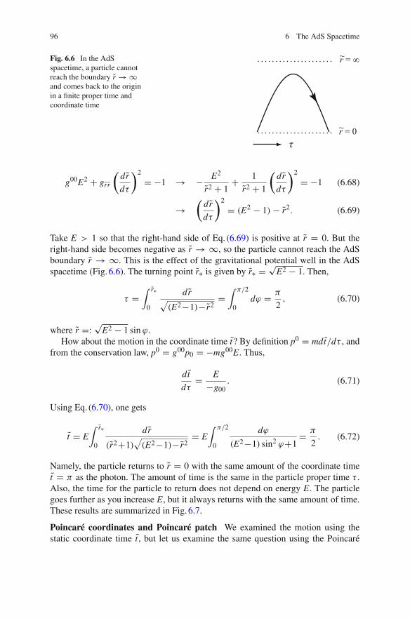
96 6 The AdS Spacetime
Fig. 6.6 In the AdSspacetime, a particle cannotreach the boundary r → ∞and comes back to the originin a finite proper time andcoordinate time
g00E2 + grr
(dr
dτ
)2
= −1 → − E2
r2 + 1+ 1
r2 + 1
(dr
dτ
)2
= −1 (6.68)
→(
dr
dτ
)2
= (E2 − 1) − r2. (6.69)
Take E > 1 so that the right-hand side of Eq. (6.69) is positive at r = 0. But theright-hand side becomes negative as r → ∞, so the particle cannot reach the AdSboundary r → ∞. This is the effect of the gravitational potential well in the AdSspacetime (Fig. 6.6). The turning point r∗ is given by r∗ = √
E2 − 1. Then,
τ =∫ r∗
0
dr√(E2−1)−r2
=∫ π/2
0dϕ = π
2, (6.70)
where r =: √E2 − 1 sin ϕ.
How about the motion in the coordinate time t? By definition p0 = mdt/dτ , andfrom the conservation law, p0 = g00p0 = −mg00E. Thus,
dt
dτ= E
−g00. (6.71)
Using Eq. (6.70), one gets
t = E∫ r∗
0
dr
(r2+1)√
(E2−1)−r2= E
∫ π/2
0
dϕ
(E2−1) sin2 ϕ+1= π
2. (6.72)
Namely, the particle returns to r = 0 with the same amount of the coordinate timet = π as the photon. The amount of time is the same in the particle proper time τ .Also, the time for the particle to return does not depend on energy E. The particlegoes further as you increase E, but it always returns with the same amount of time.These results are summarized in Fig. 6.7.
Poincaré coordinates and Poincaré patch We examined the motion using thestatic coordinate time t , but let us examine the same question using the Poincaré

6.2 Particle Motion in AdS Spacetime � 97
Fig. 6.7 The affine time and the static coordinate time t for the particle and the photon to reach theAdS boundary
coordinate time t . For simplicity, we consider only the photon motion. Consider thephoton motion from r = R to r = 0. From
ds2 = −r2dt2 + dr2
r2= 0 → dr
dt= −r2, (6.73)
one gets
t = −∫ ε
R
dr
r2= 1
r
∣∣∣∣ε
R= 1
ε− 1
R→ ∞. (6.74)
Thus, it takes an infinite coordinate time t until the photon reaches r = 0.But this is not the case in the affine parameter τ . Just like Eq. (6.67),
dr
dτ= −E, (6.75)
so it takes a finite affine time from r = R to r = 0.3
The behavior of the Poincaré coordinates is similar to the Schwarzschild coordi-nates. Because the photon reaches r = 0 in a finite affine parameter, the Poincarécoordinates cover only part of the full AdS spacetime.4 From the point of view ofthe full AdS geometry, t → ∞ as r → 0 because of the ill-behaved coordinates justlike the Schwarzschild coordinates. The region covered by Poincaré coordinates iscalled the Poincaré patch (Fig. 6.4).
In this sense, the location r = 0 is similar to the horizon but has a difference fromthe horizon. The region inside the horizon cannot influence the region outside. Butthe AdS spacetime does not have such a region. In conformal coordinates, clearlythere is no region which cannot influence the AdS boundary. The Poincaré patch israther similar to the Rindler spacetime:
ds2p+2 = −r dt2 + dr2
r+ dx2
p. (6.76)
The Rindler spacetime is just the Minkowski spacetime although it does not lookso. The difference is that the Rindler spacetime covers only part of the Minkowski
3 As in Eq. (6.67), it takes an infinite affine time from r = ∞ to r = 0, but it takes a finite amountof time from finite R to r = 0.4 Otherwise, the spacetimewould be geodesically incompletewhich signals a spacetime singularity.The geodesic incompleteness means that there is at least one geodesic which is inextensible in afinite “proper time” (in a finite affine parameter). This is the definition of a spacetime singularity.

98 6 The AdS Spacetime
spacetime. Physically, theRindler coordinates represent the observerwhoexperiencesa constant acceleration and there is a horizon, r = 0, for the observer. But the horizonis observer-dependent, and the Minkowski spacetime as a whole has no horizon.
Similarly, there is a horizon at r = 0 for the observer inside the Poincaré patch,but the AdS spacetime as a whole has no horizon. Whether r = 0 is a horizon ornot depends on the point of view.5 As a finial remark, the Rindler spacetime hasa Hawking temperature, but the AdS spacetime in Poincaré coordinates has zerotemperature. The Rindler spacetime has the following thermodynamic quantities:
T = 1
4π, s = 1
4G, ε = 0, P = 1
16πG. (6.77)
6.3 Remarks on AdS/CFT Interpretations
The symmetries of the AdS spacetime Let us rewrite the AdS5 spacetime inPoincaré coordinates6:
ds25 =( r
L
)2(−dt2 + dx2 + dy2 + dz2) + L2 dr2
r2. (6.78)
The spacetime has the SO(2, 4) invariance, part of which can be seen easily inPoincaré coordinates and are physically important:
1. Four-dimensional Poincaré invariance: The metric has the Poincaré invarianceISO(1, 3) on xμ = (t, x, y, z). This corresponds to the Poincaré invariance ofthe dual gauge theory in four-dimensional spacetime, so xμ is interpreted as thespacetime coordinates of the gauge theory. Similarly, for the AdSp+2 spacetime,p represents the number of the spatial dimensions of the dual gauge theory.
2. Four-dimensional scale invariance: The metric is invariant under
xμ → axμ, r → 1
ar. (6.79)
Under the scaling, r transforms as energy which is conjugate to t . This is onereason why the gauge theory is four-dimensional whereas the gravitational theoryis five-dimensional. Namely, the r-coordinate has the interpretation as the gaugetheory energy scale. The N = 4 SYM has the scale invariance, but the invarianceis realized geometrically in the dual gravitational theory.
5 For example, in the near-horizon limit, the extreme RN-AdS4 black hole becomes the AdS2spacetime in Poincaré coordinates (Sect. 14.3.3). In this case, r = 0 corresponds to the true horizonof the black hole. So, whether r = 0 is a true horizon or not depends on the context.6 So far we took dimensionless coordinates, but we take dimensionful ones below.

6.3 Remarks on AdS/CFT Interpretations 99
Let us examine more about the dual gauge theory energy. In AdS/CFT, the gaugetheory time corresponds to the coordinate t not to the proper time τ . The proper timeτr for the static observer at r is related to the coordinate t as
dτ 2r = |g00(r)|dt2. (6.80)
Then, the proper energy for the observer at r, E(r), is related to the gauge theoryenergy, Et , as7
Et = √|g00(r)|E(r) �( r
L
)E(r). (6.81)
Consider an excitation in theAdS spacetimewith a given proper energy (for example,a string). The gauge theory energy depends on where the excitation is located. Thegauge theory energy is larger if the excitation is nearer theAdSboundary. The relation(6.81) is called the UV/IR relation.
In general relativity, one does not put emphasis on a coordinate time since itdepends on coordinate systems. Rather one puts emphasis on the proper time. How-ever, in AdS/CFT, the coordinate time plays the special role as the gauge theory time.Thus, we use t for a gauge theory interpretation.
The Hawking temperature and the proper temperature � Similar remarks alsoapply to thermodynamic quantities of the AdS black holes in Chap.7. The Hawkingtemperature is determined from the periodicity of the imaginary time tE. This meansthat the Hawking temperature is the temperature measured by the coordinate t .
The Hawking temperature T differs from the temperature as seen by the observerat r. The proper time τr and t are related to each other by Eq. (6.80), so the propertemperature T (r) is given by
T (r) = 1√|g00(r)|T . (6.82)
For asymptotically flat black holes, the proper temperature for the asymptoticobserver coincides with the Hawking temperature since |g00| → 1 as r → ∞.But for AdS black holes, |g00| ∝ r2 as r → ∞, so the proper temperature for theasymptotic observer vanishes.8
In AdS/CFT, the coordinate t has the special interpretation as the gauge theorytime. Therefore,whenwe discuss temperatures, wewill use theHawking temperature(gauge theory temperature) not the proper temperature.
7 This equation looks similar to the gravitational redshift (6.63), but the interpretations are different.The gravitational redshift compares proper energies at different radial positions. The UV/IR relationcompares the proper energy and the energy conjugate to the coordinate t at one radial position.8 This should coincide with the surface gravity (for the asymptotic observer). When we discussedthe surface gravity, we assumed that the spacetime is asymptotically flat [in the last expressionof Eq. (3.12), we used f (∞) = 1]. For AdS black holes, the surface gravity vanishes by takingf (∞) → ∞ into account. The expression f ′(r0)/2 corresponds to the “surface gravity” in thet-coordinate.

100 6 The AdS Spacetime
6.4 Summary
• The AdS spacetime is the spacetime of constant negative curvature.• The AdS5 spacetime has the (3+1)-dimensional timelike boundary known as theAdS boundary.
• The AdS5 spacetime has the SO(2, 4) invariance. This symmetry is the same asthe (3+1)-dimensional conformal invariance of the N = 4 SYM.
• The AdS5 spacetime in Poincaré coordinates coincides with the near-horizon limitof the D3-brane.
• In AdS/CFT, the gauge theory time is the coordinate time not the proper time.Accordingly, the AdS radial coordinate has the interpretation as the gauge theoryenergy scale. Given a proper energy of an excitation, the gauge theory energy islarger if the excitation is nearer the AdS boundary.
New keywords
hyperbolic space AdS boundaryglobal coordinates de Sitter spacetimestatic coordinates maximally symmetric spacetimesconformal coordinates UV/IR relationPoincaré coordinates proper temperaturePoincaré patch

Chapter 7AdS/CFT—Equilibrium
In this chapter, we compute thermodynamic quantities for the Schwarzschild-AdS blackhole, from which one can get thermodynamic quantities of the strongly-coupled N = 4super-Yang-Mills theory. We also compare the results with the free gas result.
7.1 The AdS Black Hole
Black holes can exist in the AdS spacetime. The simplest AdS black hole is known asthe Schwarzschild-AdS black hole (SAdS black hole hereafter). Just like the Schwarz-schild black hole, one can consider AdS black holes with spherical horizon (Sect. 7.3),but we consider AdS black holes with planar horizon or AdS black branes for thetime being.
The SAdS5 black hole is a solution of the Einstein equation with a negativecosmological constant (6.62) like the AdS5 spacetime. The metric is given by
ds25 = −
( r
L
)2h(r)dt2 + dr2
( rL
)2h(r)
+( r
L
)2(dx2+dy2+dz2), (7.1)
h(r) = 1 −(r0
r
)4. (7.2)
The horizon is located at r = r0. When r0 = 0, the metric reduces to the AdS5spacetime in Poincaré coordinates (6.78). The g00 component contains the factorr4
0 /(L2r2). The O(r−2) behavior comes from the Newtonian potential which behavesas r−2 in the five-dimensional spacetime.
The coordinates (x, y, z) represent R3 coordinates. In the Schwarzschild blackhole, this part was r2dΩ2 which represents a spherical horizon, but here the r = r0horizon extends indefinitely in (x, y, z)-directions.
The AdS spacetime is a spacetime with constant curvature, but the SAdS5 blackhole is not. For example, there is a curvature singularity at r = 0.
© Springer Japan 2015M. Natsuume, AdS/CFT Duality User Guide, Lecture Notes in Physics 903,DOI 10.1007/978-4-431-55441-7_7
101

102 7 AdS/CFT—Equilibrium
The AdS spacetime is invariant under the scaling xμ → axμ, r → r/a. Underthe scaling, the SAdS black hole metric becomes
ds25 → −
( r
L
)2{
1 −(ar0
r
)4}
dt2 + · · · , (7.3)
so one can always scale the horizon radius. Namely, black holes with different horizonradii are all equivalent. As we will see, the temperature of the black hole is T ∝ r0,so one can change the temperature by the scaling. This means that all temperaturesare equivalent and the physics is the same (except at zero temperature). Thus, thereis no characteristic temperature such as a phase transition. From the gauge theorypoint of view, this is because the N = 4 SYM is scale invariant and there is nodimensionful quantity except the temperature.
Another way of saying this is that the metric is invariant under
xμ → axμ, r → 1
ar, r0 → 1
ar0. (7.4)
Using this scaling, one can obtain the functional form of the black hole temperature.The temperature T scales as the inverse time, so T → T/a under the scaling.Comparing the scaling of r0, one gets T ∝ r0. The dimensional analysis then fixesT ∝ r0/L2. See Eq. (7.8) for the numerical coefficient.
7.2 Thermodynamic Quantities of AdS Black Hole
7.2.1 Thermodynamic Quantities
Here, we compute thermodynamic quantities of the SAdS5 black hole. In AdS/CFT,they are interpreted as thermodynamic quantities of the dual N = 4 SYM at strongcoupling. In order to rewrite black hole results as gauge theory results, one needsthe relation of the parameters between two theories. This is given by the AdS/CFTdictionary in Sect. 5.3.3:
N 2c = π
2
L3
G5, λ =
(L
ls
)4
. (7.5)
On the left-hand side, we have gauge theory parameters which are written in termsof gravity parameters on the right-hand side.

7.2 Thermodynamic Quantities of AdS Black Hole 103
First, the temperature is given by
T = f ′(r0)
4π(7.6)
= 1
4π
1
L2
(2r + 2r4
0
r3
)∣∣∣∣∣r=r0
(7.7)
= 1
π
r0
L2 , (7.8)
where we used Eq. (3.26).For this black hole, the horizon has an infinite extension, and the entropy itself
diverges, so it is more appropriate to use the entropy density s. Let the spatial exten-sion of the black hole as 0 ≤ x, y, z ≤ Lx , L y, Lz . (This is just an infrared cutoffto avoid divergent expressions.) The gauge theory coordinates are (x, y, z), so thegauge theory volume is V3 := Lx L y Lz . This is different from the horizon “area”since the line element is (r/L)2(dx2 + dy2 + dz2). Then, from the area law (3.21),
S = A
4G5= 1
4G5
(r0
L
)3V3 (7.9)
or
s = S
V3= 1
4G5
(r0
L
)3. (7.10)
One would write the area law as
s = a
4G5, (7.11)
where a := A/V3 is the “horizon area density.” Using the temperature (7.8) and theAdS/CFT dictionary, one gets
s = π2
2N 2
c T 3. (7.12)
The rest of thermodynamic quantities can be determined using thermodynamic rela-tions. The first law dε = T ds can determine the energy density ε1:
ε = 3
8π2 N 2
c T 4. (7.13)
1 An integration constant is discarded. It is not allowed since we have only T as the dimensionfulquantity. This can be checked explicitly from the black hole partition function, but there are exam-ples with nonvanishing integration constants when there are other dimensionful quantities (see,e.g., Sect. 14.2).

104 7 AdS/CFT—Equilibrium
The Euler relation ε = T s − P then determines the pressure P:
P = 1
8π2 N 2
c T 4 → P = 1
3ε. (7.14)
Here, we obtained thermodynamic quantities by the area law and thermodynamicrelations, but one can obtain these quantities by evaluating the black hole free energyF(T, V3). In thermodynamics, the free energy is defined by F(T, V3) := E − T S =−P(T )V3, so the result should be
F = − V3
16πG5
r40
L5= − V3L3
16πG5π4T 4 = −1
8π2 N 2
c T 4V3 (7.15)
from Eq. (7.14), which is indeed confirmed in Appendix.This is a simple exercise, but one can learn many from the results as described
below.
The temperature dependence The temperature dependence ε ∝ T 4 representsthe Stefan-Boltzmann law. The N = 4 SYM is scale invariant, and there is nodimensionful quantity except the temperature. Then, it is obvious that we have theStefan-Boltzmann law from the field theory point of view. What is nontrivial is theproportionality constant. We will compare the coefficient with the free gas case.
However, from the black hole point of view, it is highly nontrivial that a black holeobeys the Stefan-Boltzmann law. For example, for the five-dimensional Schwarz-schild black hole, M ∝ 1/T 2, so the black hole takes a completely different formfrom the Stefan-Boltzmann form.
Moreover, the Schwarzschild black hole has a negative heat capacity C :=d M/dT < 0, and there is no stable equilibrium. Namely, the black hole emitsthe Hawking radiation, and the black hole loses its mass as the result of the radiation.This raises the temperature of the black hole, which makes the Hawking radiationmore active. In this way, the temperature becomes high indefinitely, and the blackhole does not reach an equilibrium.
The absence of the stable equilibrium is true not only for the Schwarzschild blackhole but also for a gravitational system in general. In a gravitational system, once thesystem deviates from the equilibrium, the fluctuations do not decay but grow in time,and the system deviates further from the equilibrium.2 Of course, this is one reasonwhy our universe is not uniform and is the driving force to produce astronomicalobjects such as the solar system. Thus, usual black holes cannot correspond to thestandard statistical system such as the gauge theory. The AdS black hole is veryspecial in this sense.
2 This is because the gravitational force is a long-range force. The Schwarzschild black hole can bestabilized if one confines it in a small enough “box” [1]. In the AdS black hole, there is a potentialbarrier (Sect. 6.2) which gives a natural notion of the box.

7.2 Thermodynamic Quantities of AdS Black Hole 105
Let us compare the Schwarzschild black hole and the AdS black hole more care-fully:
(5-dimensional) Schwarzschild: M � 1
G5T 2 , (7.16)
(5-dimensional) Schwarzschild-AdS: ε = (π L)3
4G5T 4. (7.17)
For the Schwarzschild black hole, there is no dimensionful quantities other than G5and T . On the other hand, for the AdS black hole, there is another dimensionfulquantity, the AdS radius L . As one can see from the AdS/CFT dictionary (7.5),L3 and G5 combine to give only a dimensionless quantity Nc. In this way, theStefan-Boltzmann law can appear for the AdS black hole. On the other hand, for theSchwarzschild black hole, one cannot eliminate the Newton’s constant G5, so theStefan-Boltzmann law cannot appear.
Also, note that the black hole entropy can be interpreted as a four-dimensionalstatistical entropy because we consider a black hole in the five-dimensional space-time. Unlike the usual statistical systems, the black hole entropy is not proportionalto the volume of the system but is proportional to the area of the horizon. That is whythe five-dimensional black hole entropy can be naturally interpreted as a (3 + 1)-dimensional quantity.
The N 2c dependence The entropy density is proportional to O(N 2
c ). This impliesthat the dual gauge theory is in the unconfined plasma phase. The entropy counts thedegrees of freedom of a system. An SU (Nc) gauge theory has O(N 2
c ) color degreesof freedom. In the unconfined phase, these contribute to the entropy. In the confinedphase, only the SU (Nc) gauge singlets contribute to the entropy, and the entropy isnot proportional to O(N 2
c ). The N = 4 SYM is scale invariant, and only the plasmaphase exists.
Traceless energy-momentum tensor The energy density and pressure satisfiesε = 3P , so the energy-momentum tensor is traceless T μ
μ = 0. This also comesfrom the scale invariance of the N = 4 SYM. The N = 4 SYM has only thetemperature as a dimensionful quantity. When thermodynamic quantities are theonly dimensionful quantities, the dimensional analysis (Stefan-Boltzmann law) andthermodynamic relations immediately imply the traceless.3
Comparison with free gas result Let us compute the entropy density for the N =4 SYM in the free gas limit in order to compare with the AdS/CFT result. First, for
3 Form the field theory point of view, the tracelessness T μμ = 0 is an operator statement and is
valid irrespective of states (either the vacuum state or a thermal state) as long as there is no traceanomaly.

106 7 AdS/CFT—Equilibrium
the photon gas, the entropy density is given by
sphoton = 2π2
45T 3 × 2 (7.18)
(Sect. 7.2.2). The last factor 2 comes from photon’s polarizations. The entropy densityfor theN = 4 SYM is given just by replacing the factor 2 with theN = 4 degrees offreedom Ndof. Let us count them. The theory has the gauge field and 6 adjoint scalars,so the bosonic degrees of freedom are Nboson = (2 + 6) × (N 2
c − 1). The theory hasthe adjoint fermions as well, but the fermionic degrees of freedom are the same as thebosonic ones from supersymmetry: Nfermion = Nboson. Also, the fermions contribute7/8 of the bosons to the entropy (Sect. 7.2.2). So, Ndof = Nboson + (7/8)Nfermion =15(N 2
c − 1). Thus, the entropy density in the free gas limit is given by
sfree = 2π2
45NdofT
3 = 2π2
3(N 2
c − 1)T 3 � 2π2
3N 2
c T 3. (7.19)
In the last equality, we took the large-Nc limit.Equations (7.12) and (7.19) have the same functional form, but the coefficients
differ [2]. They are related to each other by
sBH = 3
4sfree. (7.20)
Why the 3/4 “discrepancy”? The black hole computation or the AdS/CFT compu-tation correspond to the strong coupling result (large-Nc limit) not to the free gasresult. Namely, AdS/CFT predicts that the entropy of the N = 4 SYM at strongcoupling becomes 3/4 of the free gas result. It is difficult to check the predictionsince technical tools to compute strongly-coupled gauge theories are rather limited,but a similar behavior is obtained in lattice simulations (Chap. 12).
7.2.2 Free Gas Computation
Consider the partition function of free particles. Denote the energy level as ωi , anddenote the particle number occupying ωi as ni . The total energy of a microscopic stateis specified by n1, n2, . . . and is given by E(n1, n2, . . . ) = ∑
i niωi . The partitionfunction then becomes
Z =∑
e−βE(n1,n2,... ) =∑n1
∑n2
· · · e−β(n1ω1+n2ω2+··· ), (7.21)

7.2 Thermodynamic Quantities of AdS Black Hole 107
where β := 1/T . For bosons, ni takes the value from 0 to ∞, so
ZB =⎛⎝ ∞∑
n1=0
e−βn1ω1
⎞⎠ × · · · =
∞∏i=1
1
1 − eβωi. (7.22)
Then,
ln ZB = −∞∑
i=1
ln(1 − e−βωi ) (7.23)
→ −V∫
d3q
(2π)3 ln(1 − e−βω) (7.24)
= − V
(2π)3 4π
∫ ∞
0dq q2 ln(1 − e−βq) (7.25)
= − V
2π2
1
β3
∫ ∞
0dx x2 ln(1 − e−x ), (x := βq) (7.26)
= Vπ2
90β3 . (7.27)
Here, we replaced the sum by the integral in Eq. (7.24) by taking the V → ∞ limit.We also used the dispersion relation ω = |q| for massless particles in Eq. (7.25).The integral in Eq. (7.26) (as well as the corresponding integral for fermions below)is evaluated as
∫ ∞
0dx x2 ln(1 − e−x ) = −π4
45,
∫ ∞
0dx x2 ln(1 + e−x ) = 7π4
360. (7.28)
Therefore, thermodynamic quantities are given by
εB = − 1
V
∂ ln ZB
∂β= π2
30β4 , (7.29)
sB = 1
Vln ZB + βεB = 2π2
45β3 . (7.30)
Similarly, for fermions, ni takes the value either 0 or 1, so
ZF = (1 + eβω1) × · · · =∞∏
i=1
(1 + eβωi ), (7.31)
ln ZF =∞∑
i=1
ln(1 + e−βωi ) (7.32)

108 7 AdS/CFT—Equilibrium
→ V∫
d3q
(2π)3 ln(1 + e−βω) (7.33)
= V
(2π)3 4π
∫ ∞
0dq q2 ln(1 + e−βq) (7.34)
= V7π2
720β3 . (7.35)
Thus,
ln ZF = 7
8ln ZB. (7.36)
7.3 The AdS Black Hole with Spherical Horizon
The AdS black hole with spherical horizon is given by
ds25 = −
(r2
L2 + 1 − r40
L2r2
)dt2 + dr2
r2
L2 + 1 − r40
L2r2
+ r2dΩ23 . (7.37)
When r0 = 0, the metric reduces to the AdS5 metric in static coordinates. Thehorizon is located at r = r+, where
r2+L2 + 1 − r4
0
L2r2+= 0 → r4
0 = r4+ + L2r2+. (7.38)
Unlike the planar horizon case, black holes with different horizon radii are inequiv-alent. In particular, the large black hole limit corresponds to the planar horizon case(7.1). To see this, consider the scale transformation t → at , r → r/a and takethe a → 0 limit. We want to consider the large black hole limit, but we keep thecoordinate value r+ of the horizon fixed under the scale transformation. To do so,transform r+ → r+/a or r0 → r0/a [we consider the large black hole limit, so takeonly the O(r4+) term in Eq. (7.38) into account]. Then,
ds25 → −
(r2
L2 + a2− r40
L2r2
)dt2 + dr2
r2
L2 +a2− r40
L2r2
+( r
a
)2dΩ2
3 . (7.39)
The metric does not reduce to Eq. (7.37) under the scaling. The radius of the S3
horizon grows as r/a. In the a → 0 limit, the horizon becomes flat, and one canapproximate (r/a)2dΩ2
3 � (r/L)2dx23 usingR3 coordinates. The resulting geometry
is the planar horizon one.

7.3 The AdS Black Hole with Spherical Horizon 109
Black holes with different horizon radii are inequivalent, so not all temperaturesare equivalent. In fact, we will see in Sect. 14.2 that a phase transition can occur forthe black hole.
Remark Readers do not have to worry much at this point, but we mainly focus onthe planar horizon in this book from the following reasons.
• As we saw in Chap. 5 App. 2, the near-horizon limit of the D3-brane gives theblack hole with planar horizon.
• The coordinates (x, y, z) correspond to the gauge theory spatial coordinates, so ablack hole with planar horizon corresponds to a standard gauge theory on R
3. Ablack hole with compact horizon corresponds to a gauge theory on compact space.It is interesting in its own right because it has rich physics such as phase transition.To put differently, such a black hole is more complicated, so we postpone thediscussion.
• In later chapters, we add perturbations to black holes and take the low-energyω → 0, long-wavelength limit q → 0 for hydrodynamic analysis of large-Nc
plasmas. But for a black hole with compact horizon, the wavelength of the pertur-bation necessarily becomes the black hole scale.To be more precise, let us consider the perturbation of a field φ on black hole back-grounds. For the planar horizon, we can decompose the perturbation as the planewave, φ ∝ e−iωt+iqz . In this case, one can take the ω → 0, q → 0 limits. For thespherical horizon, we decompose the perturbation using spherical harmonics. ForS2 horizon, φ ∝ Ylm(θ, ϕ). As a result, the spectrum is discrete so that we cannottake the limit.
7.4 Summary
• In the AdS5 spacetime, a black hole with planar horizon exists. We consider blackholes with planar horizon from various reasons.
• The SAdS5 black hole (with planar horizon) obeys the (3+1)-dimensional Stefan-Boltzmann law like a standard statistical system.
• The entropy of the (4 + 1)-dimensional black hole is interpreted as a (3 + 1)-dimensional quantity because of the area law of the black hole entropy.
• The entropy of the SAdS5 black hole is 3/4 of the entropy of the N = 4 SYMin the free gas limit. This implies that the entropy of the N = 4 SYM at strongcoupling becomes 3/4 of the free gas entropy.
New keywords
Schwarzschild-AdS black hole [extrinsic/intrinsic curvature]Stefan-Boltzmann law [counterterm action][Gibbons-Hawking action] [holographic renormalization]

110 7 AdS/CFT—Equilibrium
Appendix: AdS Black Hole Partition Function �
In this section, we evaluate the semiclassical partition function for the SAdS5 blackhole. The partition function gives thermodynamic quantities in Sect. 7.2.4
First of all, the gravitational action is schematically written as
SE = Sbulk + SGH + SCT. (7.40)
Here, Sbulk, SGH, and SCT are called the bulk action, the Gibbons-Hawking action,and the counterterm action, respectively. We explain these actions below and evaluateon-shell actions for the SAdS5 black hole. We use the following coordinates:
ds25 =
( r
L
)2(hdt2
E + dx23) + L2 dr2
hr2 , h = 1 −(r0
r
)4, (7.41)
=(r0
L
)2 1
u2 (hdt2E + dx2
3) + L2 du2
hu2 , h = 1 − u4, (7.42)
(u := r0/r ). Note that we consider Euclidean actions and the Euclidean metrichere.5 In the coordinate r , the black hole “horizon” is located at r = r0 and theAdS boundary is located at r = ∞. In the coordinate u, the black hole “horizon” islocated at u = 1 and the AdS boundary is located at u = 0.
The bulk action The bulk action is the five-dimensional action. For the SAdSp+2black hole, it is the standard Einstein-Hilbert action:
Sbulk = − 1
16πG p+2
∫d p+2x
√g (R − 2Λ) , (7.43)
2Λ = − p(p + 1)
L2 . (7.44)
The SAdS5 black hole corresponds to p = 3. The contraction of the Einstein equation
RMN − 1
2gMN R + ΛgMN = 0 (7.45)
gives
R = − (p + 1)(p + 2)
L2 . (7.46)
4 �There are actually several ways to compute thermodynamic quantities. For example, one canuse the Brown-York tensor [3]. Or one can read them directly from the “fast falloff” of the metric(Chap. 10). These methods are simpler but are essentially equivalent to the method here. In thisbook, we always start from the GKP-Witten relation if possible. You would learn these alternativemethods once you get accustomed to AdS/CFT computations.5 The Lorentzian action SL and the Euclidean action SE are related by iSL = i
∫dtL =
− ∫dtE(−L) = −SE from tE = i t .

Appendix: AdS Black Hole Partition Function � 111
Thus, the on-shell bulk action6 is
Sbulk = p + 1
8πG p+2 L2
∫d p+2x
√g, (7.47)
i.e., it is proportional to the spacetime volume. For the SAdS5 black hole,
Sbulk = 1
2πG5
r40
L5
∫ β
0dt
∫dx
∫ 1
udu
1
u5(7.48)
u→0−−−→ βV3
8πG5
r40
L5
(1
u4 − 1
)∣∣∣∣∣u=0
(7.49)
=: βV3
16πG5
r40
L5Sbulk, (7.50)
where V3 is the volume of x-directions. One can check that the factor in front ofSbulk is common to the other on-shell actions, so we will set β = V3 = r0 = L =16πG5 = 1 below.
The bulk action diverges as u → 0 because it is proportional to the spacetimevolume.
The Gibbons-Hawking action It is necessary to add the following “surface term”to the Einstein-Hilbert action in order to have a well-defined variational problem (seeChap. 12 App. 1):
SGH = − 2
16πG p+2
∫d p+1x
√γ K . (7.51)
The action is known as the Gibbons-Hawking action. This is a surface term evaluatedat u = 0. Here, γμν is the (p + 1)-dimensional metric at the surface, and K is thetrace of the extrinsic curvature of the surface as described below.
This is a surface term, so it does not affect the equation of motion (Einstein equa-
tion), but it does affect the value of the on-shell action. Elementary general relativitytextbooks rarely put emphasis on the Gibbons-Hawking action since the equation ofmotion is fundamentally important for the dynamics of curved spacetimes. But forthermodynamic properties, one is interested in the whole value of the on-shell actionin the Euclidean formalism, so this action is equally important.
Moreover, in some cases, it is the only contribution to the on-shell action. Forthe Schwarzschild black hole, R = 0, so the bulk action makes no contribution tothe on-shell action. The contribution to the on-shell action entirely comes from theGibbons-Hawking action.
6 We write on-shell actions S as S below for simplicity.

112 7 AdS/CFT—Equilibrium
Fig. 7.1 For the cylinder,the intrinsic curvaturevanishes (R = 0), but theextrinsic curvature can benonvanishing (K = 0) R = 0
K 0
For simplicity, consider a diagonal metric such as the SAdS black hole. The(p + 1)-dimensional metric γμν is given by decomposing the metric as (“The ADMdecomposition”)
ds2p+2 = guudu2 + γμνdxμdxν . (7.52)
The unit normal to the u = (constant) surface is given by7
gMNnM nN = 1 → nu = − 1√guu
. (7.53)
Then, K is given by8
K = nu ∂u√
γ√γ
. (7.55)
There are two kinds of curvature: intrinsic and extrinsic. The Riemann tensoris the former. The extrinsic curvature relies on the notion of a higher-dimensionalspacetime. Namely, the extrinsic curvature of a spacetime relies on how the spacetimeis embedded into a higher-dimensional spacetime. The Riemann tensor does not haveto assume the existence of such a higher-dimensional spacetime.
For example, consider a cylinder (Fig. 7.1). The cylinder has no intrinsic curvatureR = 0 since the cylinder is just a flat space with a periodic boundary condition. Butthe cylinder is “curved.” This is the curvature which arises by embedding it into thethree-dimensional space. This is the extrinsic curvature. In cylindrical coordinates
ds2 = dz2 + dr2 + r2dθ2, (7.56)
7 The vector nM is “outward-pointing” pointing in the direction of decreasing u or increasing r .8 For a diagonal metric, the extrinsic curvature itself is given by
Kμν = 1
2nu∂uγμν, (7.54)
and the trace is defined by K := γ μν Kμν . Use the matrix formula (2.68) ∂μ(det M) =det M tr(M−1∂μM) to derive Eq. (7.55) from Kμν .

Appendix: AdS Black Hole Partition Function � 113
the cylinder is the r = (constant) surface. Then, nr = 1, γμν = diag(1, r2), and√γ = r , so the extrinsic curvature is indeed nonvanishing K = 1/r .In general relativity, one considers the extrinsic curvature of a surface when one
embeds the surface into a spacetime or when one discusses the canonical formalism(one slices the spacetime into a series of spacelike hypersurfaces). In our case, weare talking of the extrinsic curvature of the four-dimensional timelike hypersurfacesliced at u = (constant) of the five-dimensional AdS black hole. This hypersurfaceis the spacetime where the boundary gauge theory lives.
For the SAdS5 black hole, nu = −uh1/2 and√
γ = u−4h1/2, so
SGH = 2uh1/2[u−4h1/2
]′∣∣∣∣u=0
u→0−−−→ − 8
u4 + 4
∣∣∣∣u=0
. (7.57)
Note that the Gibbons-Hawking action also diverges as u → 0.
The counterterm action As we saw above, the bulk action and the Gibbons-Hawking action diverge as u → 0. To cancel the divergence, we add to the actionanother surface term, the counterterm action.
In AdS/CFT, this divergence is interpreted as the ultraviolet divergence of the dualfield theory. In the dual field theory, it is clear how to handle the divergence. Onecarries out the renormalization and adds a finite number of local counterterms to thebare action. Following this field theory prescription, we add a counterterm action inorder to have a finite gravitational partition function. This procedure is known as theholographic renormalization.9
Thus, the counterterm action is chosen so that
• It is written only in terms of boundary quantities (γμν and the quantities made ofγμν such as the Ricci scalar10 R).
• It consists of only a finite number of terms.• The coefficients of these terms are chosen once and for all in order to cancel
divergences.
When p ≤ 5, the counterterm action is given by
SCT = 1
16πG p+2
∫d p+1x
√γ
{2p
L+ L
p − 1R
− L3
(p − 3)(p − 1)2
(RμνRμν − p + 1
4pR2
)+ · · ·
}. (7.58)
9 See, e.g., Ref. [4] for a review of the holographic renormalization. The counterterm action containsthe AdS scale L , so one cannot regulate the divergence if the spacetime is not asymptoticallyAdS. In particular, one cannot use this prescription for asymptotically flat black holes such as theSchwarzschild black hole. See Sect. 14.2 for a prescription of such a case.10 Readers should not confuse R with R, the Ricci scalar in the bulk spacetime. RMN is a tensor in(p + 2)-dimensions, and Rμν is a tensor in the (p + 1)-dimensions.

114 7 AdS/CFT—Equilibrium
The above terms are enough to cancel power-law divergences for p ≤ 5, but one mayneed the other terms to cancel log divergences. For black holes with planar horizon,Rμν = 0, so only the first term contributes to thermodynamic quantities:
SCT = 6u−4h1/2∣∣∣u=0
u→0−−−→ 6
u4 − 3
∣∣∣∣u=0
. (7.59)
The partition function and thermodynamic quantities To summarize our results(7.49), (7.57), and (7.59),
Sbulk = 2
u4 − 2
∣∣∣∣u=0
, (7.60)
SGH = − 8
u4 + 4
∣∣∣∣u=0
, (7.61)
SCT = 6
u4 − 3
∣∣∣∣u=0
. (7.62)
Combining these results, we get a simple result Sbulk + SBH + SCT = −1 after allthese computations. Recovering dimensionful quantities, we get
SE = − βV3
16πG5
r40
L5. (7.63)
The on-shell action is related to the partition function Z and the free energy F as
Z = e−SE , SE = βF. (7.64)
Then, the free energy becomes
F = − V3
16πG5
r40
L5= − (π LT )4
16πG5LV3 = −1
8π2 N 2
c T 4V3, (7.65)
where we used T = r0/(π L2). Thermodynamic quantities are then derived from thefree energy as
s = − 1
V3∂T F = (π LT )3
4G5= 1
4G5
(r0
L
)3 = 1
2π2 N 2
c T 3, (7.66)
P = −∂V3 F = (π LT )4
16πG5L= 1
16πG5L
(r0
L
)4 = 1
8π2 N 2
c T 4, (7.67)
ε = F
V3+ T s = 3(π LT )4
16πG5L= 3
16πG5L
(r0
L
)4 = 3
8π2 N 2
c T 4. (7.68)

References 115
References
1. J.W. York Jr., Black hole thermodynamics and the Euclidean Einstein action. Phys. Rev. D33,2092 (1986)
2. S.S. Gubser, I.R. Klebanov, A.W. Peet, Entropy and temperature of black 3-branes. Phys. Rev.D54, 3915 (1996). arXiv:hep-th/9602135
3. V. Balasubramanian, P. Kraus, A stress tensor for anti-de Sitter gravity. Commun. Math. Phys.208, 413 (1999). arXiv:hep-th/9902121
4. K. Skenderis, Lecture notes on holographic renormalization. Classical Quantum Gravity. 19,5849 (2002). arXiv:hep-th/0209067

Chapter 8AdS/CFT—Adding Probes
In real experiments, one often adds “probes” to a system to examine its response. Or oneadds impurities to a system to see how they change the properties of the system. In thischapter, we discuss how to add probes in AdS/CFT. As a typical example, we add “quarks”to gauge theories as probes and see the behavior of quark potentials.
Coupling new degrees of freedom to the original system often arises new phenomena.Adding some new degrees of freedom to AdS/CFT should be also interesting. Thisis practically important as well. The N = 4 SYM is clearly insufficient to mimicreal worlds completely since, e.g., it does not have quarks.
In string theory, there are various fields and branes, so one may would like to addthem. The resulting geometries or solutions have been known for some cases, butit is in general very difficult to solve the Einstein equation when there are multiplenumber of fields and branes.
So, one often adds them as “probes.” This is just like the particle motion analy-sis in curved spacetime (Sects. 2.3 and 6.2). One fixes the background geometryand considers the case where the backreaction of the probe onto the geometry isnegligible.
In this chapter, as a typical example, we add “quarks” to large-Nc gauge theoriesas a probe and analyze quark potentials. In Sect. 14.3, we see another example of aprobe system, holographic superconductors.
8.1 Basics of Wilson Loop
The Wilson loop is an important observable in gauge theory, and it represents thequark-antiquark potential physically. As an example, consider a U (1) gauge theorywith gauge transformation given by
φ(x) → eiα(x)φ(x), (8.1)
Aμ(x) → Aμ(x) + ∂μα(x). (8.2)
© Springer Japan 2015M. Natsuume, AdS/CFT Duality User Guide, Lecture Notes in Physics 903,DOI 10.1007/978-4-431-55441-7_8
117

118 8 AdS/CFT—Adding Probes
Fig. 8.1 a Path P . b TheWilson loop represents aquark-antiquark pair
(a) (b)
A nonlocal operator such as φ(x)φ∗(y) is not gauge invariant in general and is notan observable. But the following quantity is gauge-invariant:
φ(x)ei∫
P dxμ Aμφ∗(y), (8.3)
where P is an arbitrary path from point x to y (Fig. 8.1a). It transforms as
φ(x)ei∫
P dxμ Aμφ∗(y) → φ(x)eiα(x)ei∫
P dxμ(Aμ+∂μα)e−iα(y)φ∗(y) (8.4)
= φ(x)ei∫
P dxμ Aμφ∗(y). (8.5)
Or if one takes a closed path P , WP itself is gauge invariant. Thus, we define thefollowing operator:
WP (x, y) = ei∫
P dxμ Aμ (Wilson line), (8.6)
WP (x, x) = ei∮
dxμ Aμ (Wilson loop). (8.7)
The Wilson loop represents the coupling of the gauge field to a test charge. Con-sider a charged particle with world-line yμ(λ). The current is given by
Jμ(x) =∮
dλdyμ
dλδ(xμ − yμ
(λ))
. (8.8)
The sign of the charge depends on the sign of dy/dλ. Here, we take dy/dλ > 0 for apositive charge. For a given closed path, dy/dλ can be both positive and negative, sowe have both a positive charge and a negative charge (Fig. 8.1b). Namely, the closedpath describes the process of creating a “quark-antiquark pair” from the vacuum,pulling them a distance R apart, interacting for time T , and annihilating them. Ifone uses Jμ, the coupling of the gauge field to the point particle action is written asδS = ∫
d4x Aμ Jμ. This perturbed action δS can be rewritten as the exponent of the

8.1 Basics of Wilson Loop 119
Wilson loop:
δS =∫
d4x Aμ(x)Jμ(x) =∮
dλdyμ
dλAμ(y(λ)) =
∮dyμ Aμ(y). (8.9)
Therefore, the Wilson loop represents a partition function in the presence of a testcharge:
〈WP 〉 = Z [J ]Z [0] . (8.10)
Such a partition function gives the quark-antiquark potential. Let us write theEuclidean partition function formally as
Z = 〈 f |e−HT |i〉 (8.11)
(|i〉 and | f 〉 are the initial state and the final state, respectively). If one uses a completeset of energy eigenstates H |n〉 = En|n〉,
Z =∑
n
e−EnT 〈 f |n〉〈n|i〉 T →∞−−−−→ e−E0T . (8.12)
Thus, in the T → ∞ limit, the Euclidean partition function is dominated by theground state and gives the ground state energy. When the kinetic energy is negligible,it gives the quark-antiquark potential energy.1 Consequently,
〈WP 〉 � e−V (R)T . (8.13)
One can show that the horizontal parts of Fig. 8.1b are negligible in the largeT → ∞limit.
When the quark is confined like QCD, the potential grows with the separation R,so V (R) � σR(R � 1), where σ is called the string tension. Then,
〈WP 〉 � e−O(RT ) = e−σ A. (8.14)
The exponent is proportional to the area of the Wilson loop A = RT . This behavioris known as the area law. An unconfined potential behaves differently. The Coulombpotential decays with the separation, and one can show that
〈WP 〉 � e−O(R) (when R = T � 1). (8.15)
This is known as the perimeter law. In this way, the Wilson loop provides a criterionfor the confinement.
1 From tE = i t , the Lorentzian action SL , the Euclidean action SE , and the potential V are relatedto each other by iSL = i
∫dt (−V ) = − ∫
dtEV = −SE .

120 8 AdS/CFT—Adding Probes
Here, we consider only the U (1) gauge theory, but a similar discussion can bedone for a Yang-Mills theory.
8.2 Wilson Loops in AdS/CFT: Intuitive Approach
Let us consider the Wilson loop in AdS/CFT. The Wilson loop in AdS/CFT givesa typical example of adding a probe system to the original system. The AdS/CFTresults can be understood intuitively. So, before we go through an actual computation,we first explain what kind of results one can expect in various situations. Then, weconfirm our intuitive explanation via an actual computation.
The matter fields in the N = 4 SYM are all in the adjoint representation. So,one first has to understand how to realize the fundamental representation such as aquark in AdS/CFT. Below, we describe one simple way to add such matter.
To do so, recall how the adjoint representation appeared for the D-brane (Fig. 8.2a).The open strings can have endpoints on a D-brane, but when there are multiplenumber of D-branes, an open string can have endpoints in various ways; there areN 2
c possibilities. This means that the string transforms as the adjoint representationof SU (Nc) gauge theory.
Now, consider an infinitely long string (Fig. 8.2b). In this case, the string canhave endpoints in Nc different ways. This means that the string transforms as thefundamental representation of SU (Nc) gauge theory. In this sense, such a long stringrepresents a “quark.” Such a string has an extension and tension, so the string has alarge mass, which means that the long string represents a heavy quark. We discussthe Wilson loop in AdS/CFT using such a string.
We saw earlier that the string model of QCD does not describe potentials otherthan the confining potential (Problem 2 of Sect. 5.1). However, one can avoid thisproblem in AdS/CFT, and one can get the Coulomb potential which appears at shortdistances in QCD. The AdS/CFT result differs from the simple string model oneessentially because of the curved spacetime effect as discussed below. Note that weavoided Problem 1 of Sect. 5.1 by the same trick.
First, we discuss the simplest case, the pure AdS case, to understand the basic ideaof the AdS/CFT quark potential. In this case, one gets only the Coulomb potential.We then consider a more generic AdS spacetime and get a confining potential aswell. Also, if we consider a black hole, we can recover behaviors in plasma phase.
Fig. 8.2 a An open stringcan have endpoints on aD-brane. The Nc coincidentD-branes represent aSU (Nc) gauge theory.b A long string represents amassive “quark”
(a) (b)

8.2 Wilson Loops in AdS/CFT: Intuitive Approach 121
The pure AdS spacetime The AdS metric in Poincaré coordinates is written as
ds2 =( r
L
)2(−dt2 + dx2 + · · · ). (8.16)
The line element has the factor r2. We measure the gauge theory time and distanceusing t and x , but they differ from the proper time and distance of the AdS spacetime.This is the important point, and the qualitative behavior of the quark potential canbe understood using this fact.
Figure 8.3 shows the AdS spacetime schematically. Denote the quark-antiquarkseparation as Δx = R. The quark-antiquark pair is represented by a string whichconnects the pair. The string has the tension, so the tension tends to minimizes thestring length. At first glance, one would connect the pair by a straight string at r = ∞(Fig. 8.4). But this does not minimize the string length. This is because the coordinatedistance does not represent a true distance (proper distance) in a curved spacetime.The figure does not show the proper length properly, so one needs a care. For theAdS spacetime, the proper length of the string actually gets shorter if the string goesinside the AdS spacetime (r = ∞). The line element has the factor r2, so the properlength rΔx gets shorter near the origin.
r = 0
r =
x
r
Fig. 8.3 Schematically drawn AdS spacetime. The horizontal direction represents one of three-dimensional space the gauge theory lives. The vertical direction represents the AdS radial coordinate.The radial coordinate extends from r = 0 to r = ∞, but we draw in a compact region for illustration
Fig. 8.4 The straight string is not the lowest energy state (left), and the string which goes insidethe AdS spacetime is the lowest energy state (right)

122 8 AdS/CFT—Adding Probes
Fig. 8.5 The string whichconnects the quark pair (left)is approximated by arectangular string. Theenergy of the horizontalstring gives the quarkpotential
potential part
r =
r = 0
According to the analysis of Sect. 8.4, this string is roughly divided into two parts:the part the string extends vertically, and the part the string extends horizontally. So,for simplicity, let us approximate the configuration by a rectangular string (Fig. 8.5).Only the horizontal string contributes to the quark potential. This part varies as wevary the quark separation R. On the other hand, the vertical string does not varymuch. This part simply describes the quark mass.
We need a little more information to compute the potential. The explicit compu-tation shows that the string turning point r = rm behaves as
rm ∝ L2/R (8.17)
(Fig. 8.6). Also, the line element (8.16) gives two consequences. First, the properlength of the horizontal string is (r/L)R, so the string energy E(r) is given by
E(r) ∝( r
L
)R. (8.18)
Second, this energy is the proper energy and not the gauge theory energy. The timelikedirection also has the factor r2 as in Eq. (8.16). The gauge theory time is the coordinatetime t not the proper time. As a result, the gauge theory energy differs from the properenergy E(r). From Eq. (8.16), the proper time τr is related to the gauge theory timeby τr = (r/L)t , so the proper energy is related to the gauge theory energy Et by
Et =( r
L
)E(r). (8.19)
Fig. 8.6 The behavior of thestring as we vary the quarkseparation. The larger Rlowers the string turningpoint rm as rm ∝ 1/R
r =
r = 0

8.2 Wilson Loops in AdS/CFT: Intuitive Approach 123
This is the UV/IR relation in Sect. 6.3 [1, 2]. Thus, the potential is given by
Et =(rm
L
)E(r) ∝
(rm
L
)2R (8.20)
∝ L2
R, (8.21)
where we also used Eq. (8.17). This result [3, 4] has two important points:
1. First, we obtained the Coulomb potential E ∝ 1/R not the confining potentialE ∝ R. Namely, the string connecting the quark-antiquark pair does not neces-sarily implies a confining potential, but it can describe an unconfining potentialusing the curved spacetime. In this way, we resolved Problem 2 of the string modelin Sect. 5.1. But then, how can we describe the confining potential in AdS/CFT?We will discuss this point below.
2. Second, the potential is proportional to L2. According to the AdS/CFT dictionary,L2 ∝ λ1/2, so the potential is proportional to (g2
YM Nc)1/2. But perturbatively, the
potential is proportional to g2YM Nc. This is because the AdS/CFT result corre-
sponds to the large-Nc limit and represents a nonperturbative effect.2
Let us evaluate the potential for a generic metric for later use. By repeating theabove argument, the potential energy becomes
Et = √−g00|rm E(r) = 1
2πl2s
√−g00gxx |rm R, (8.22)
where the metric is evaluated at r = rm . We also included the factor of the stringtension T = 1/(2πl2
s ) which we ignored in Eq. (8.18).
The confining phase AdS/CFT can also describe the confining potential which theold string model can describe qualitatively well. The pure AdS spacetime correspondsto theN = 4 SYM not to QCD. TheN = 4 SYM is scale invariant and the confiningphase does not exist even at zero temperature. We need to modify the simple AdSgeometry to describe a theory which is closer to QCD.
Many examples are known about how the AdS spacetime is deformed if onedeforms the N = 4 SYM. But we use a simple model to simplify our analysis here[7]. The AdS spacetime extends from r = ∞ to r = 0, but in this model, we cut offthe AdS spacetime at r = rc (Fig. 8.7). Let us suppose that the confinement happensat a low-energy scale Λ. In AdS/CFT, the r -coordinate has the interpretation as thegauge theory energy scale. So, the confinement means that the AdS spacetime is
2 For the N = 4 SYM at zero temperature, the potential is evaluated nonperturbatively from thefield theory point of view, and it indeed behaves as λ1/2 at strong coupling [5, 6].

124 8 AdS/CFT—Adding Probes
Fig. 8.7 In the cutoff AdSspacetime, the string reachesthe end of the space, r = rc,when the quark separation islarge enough
r = rc
r =
Fig. 8.8 The plasma phasecase. The shaded regionrepresents the black hole
r = r0
r =
r = 0
modified deep inside the AdS spacetime r ∝ Λ. The cutoff AdS roughly representsthis effect.3
Even though we modify the spacetime, there is little difference if the string is farenough from the cutoff r = rc. One gets the Coulomb potential like the pure AdSspacetime. But if the quark separation R is large enough, there is a new effect.
In the AdS spacetime, the turning point of the string behaves as rm ∝ 1/R. But inthe cutoff AdS spacetime, the string reaches at r = rc for a large enough R. Once thestring reaches there, the string cannot go further. Thus, from Eq. (8.22), the energyof the horizontal string is given by
Et ∝ r2c R � O(R), (8.23)
which is indeed the confining potential.After all, what contributes to the potential energy is the string at the cutoff
r = rc, so the AdS/CFT computation essentially reduces to the old string modelone. AdS/CFT takes the advantage of the old string model and at the same timeovercomes the difficulty of the model.
The plasma phase We now consider the finite temperature case or the plasmaphase. According to AdS/CFT, the N = 4 SYM at finite temperature correspondsto the AdS black hole (Fig. 8.8).
At finite temperature, there is a black hole horizon at r = r0. But if the string is farenough from the black hole, the geometry is approximately the AdS spacetime, soone approximately has the Coulomb potential. But if the string reaches the horizon,there is a new effect.
3 The cutoff AdS is a toy model for the confinement, but we discuss an explicit example in Appendix.

8.2 Wilson Loops in AdS/CFT: Intuitive Approach 125
For a black hole, the line element in the timelike direction has the unique behavior,and the relation (8.19) between E(r) and Et is modified. For the Schwarzschild-AdS5(SAdS5) black hole, the line element is given by
ds2 = −( r
L
)2{
1 −(r0
r
)4}
dt2 + · · · , (8.24)
so g00 = 0 at the horizon r = r0. Thus, Eq. (8.22) gives
Et = 0. (8.25)
Namely, the horizontal string has no contribution to the energy. Thus, there is noforce when the quark separation is large enough. This is the Debye screening inAdS/CFT [8–10].
Return of Wilson loops The Wilson loop argument here was proposed in lessthan two weeks after the systematic AdS/CFT researches started in 1998. Variousextensions were made within a month. But people started to come back to such simpleanalysis since 2006.
What changed the situation? In the past, such a computation was made to findcircumstantial evidences of AdS/CFT. Namely, one would like to check whetherAdS/CFT correctly reproduces the behavior of gauge theories or not. People do notreally have real applications in mind. This is understandable since supersymmetricgauge theories are different from QCD, so probably one was reluctant to apply themto the “real world.” But in recent years, people revisits such analysis and computevarious effects by taking into account the real experimental situations.
As discussed in Sect. 4.1.2, the perturbative QCD is not very effective even in theplasma phase. Thus, heavy-ion physicists try to identify the typical “fingerprints” ofQGP. Some of the fingerprints discussed to date are
1. Small shear viscosity (Chaps. 4 and 12)2. Jet quenching3. J/Ψ -suppression
In the parton hard-scattering, jets are often formed. A jet is a collection of hadronswhich travel roughly in the same direction. If jets are formed in the plasma medium,the energy of the jets are absorbed by the medium, so the number of observed hadronsare suppressed. This is the jet quenching (Fig. 8.9).
Another fingerprint is the J/Ψ -suppression [11]. J/Ψ is a “charmonium” whichconsists of cc. Since a charm quark is heavy (≈4.2 GeV), the charm pair productionoccurs only at the early stage of heavy-ion collisions. Now, if the production occursin the plasma medium, the interaction between cc is screened by the light quarks andgluons in between, which is the Debye screening. Then, the charm quark is morelikely to bind with the plasma constituents rather than the charm antiquark. The resultis the suppression of J/Ψ production.
These phenomena have been discussed in AdS/CFT. For example, consider thejet quenching [12–17]. So far, we considered the static quark to obtain the potential.

126 8 AdS/CFT—Adding Probes
Fig. 8.9 Left The collisionof nuclei in vacuum. RightJet quenching in the plasma.The ellipsoid represents theplasma
?
Jets
Fig. 8.10 Jet quenching inAdS/CFT
v
energy
r =
r = r0
r = 0
But in this case, one is interested in how the quark loses its energy. So, move thequark (string) with velocity v along the x-direction. Then, the string is dragged as inFig. 8.10. The string is dragged because the energy of the string flows towards thehorizon. This energy loss is interpreted as the energy loss of the quark in the plasmamedium.
8.3 String Action
In order to confirm the intuitive explanation in the last section, let us first consider thestring action. The string action is obtained using the similar argument as the particleaction in Sect. 2.1. A particle draws a world-line in spacetime. Similarly, a stringsweeps a two-dimensional surface, a world-sheet, in spacetime (Fig. 8.11). We writethe particle action by the proper length of the world-line. Similarly, it is natural towrite the string action by the area A of the world-sheet:
S = −T∫
d A. (8.26)
The parameter T has the dimensions [T] = L−2, which makes the action dimen-sionless. Physically, it represents the string tension. It is convenient to introduce a

8.3 String Action 127
Fig. 8.11 A string sweeps aworld-sheet in spacetime
0
1
x0
x1
parameter ls with the dimension of length and to write the tension as
T = 1
2πl2s. (8.27)
The parameter ls represents the characteristic length scale of the string (string length).Just as the particle action, introduce coordinates σ a = (σ 0, σ 1) on the world-
sheet. Then, the world-sheet is described by x M (σ a). Using the world-sheet coordi-nates σ a , the spacetime metric is written as
ds2 = ηMN dx M dx N = ηMN∂x M
∂σ a
∂x N
∂σ bdσ adσ b (8.28)
=: hab dσ adσ b, (8.29)
where hab is known as the induced metric. What we are doing here is essentiallythe same as the embedding of a hypersurface into a higher-dimensional spacetime inChap. 6. For example, embed S2 into R
3:
ds2 = d X2 + dY 2 + d Z2 = dθ2 + sin2 θ dϕ2 (8.30)
In this case, we take S2 coordinates as σ a = (θ, ϕ), and the induced metric is givenby
hab =(
1 00 sin2 θ
). (8.31)
Using the world-sheet coordinates, one can write the area element as
d A = d2σ√−det hab. (8.32)

128 8 AdS/CFT—Adding Probes
For S2, d A = sin θ dθ dϕ, which is the familiar area element for S2. The coordinatesσ a are just parameterizations on the world-sheet, so the area element is invariantunder
σ a′ = σ a′(σ b). (8.33)
The situation is similar to general relativity. In general relativity, one writes thevolume element as dd x
√−g, and the volume element is invariant under coordinatetransformations. The only difference is whether one considers a spacetime or a world-sheet. In general relativity, one considers the volume element in spacetime and thecoordinate transformation in spacetime, whereas Eq. (8.32) is the area element onthe world-sheet and Eq. (8.33) is the coordinate transformation on the world-sheet.
Using Eq. (8.32), one gets the Nambu-Goto action:
SNG = −T∫
d2σ√− det hab. (8.34)
From Eq. (8.28), the induced metric is written as
hab =(
x · x x · x ′x · x ′ x ′ · x ′
) (˙ := ∂σ 0 , ′ := ∂σ 1). (8.35)
Just as in Eq. (8.31), this is a matrix on (a, b) indices. Using this, we can write theNambu-Goto action as
SNG = −T∫
d2σ√
(x · x ′)2 − x2x ′2. (8.36)
One can consider a few extensions of the action:
1. Here, we used the Minkowski spacetime as the ambient spacetime. But one canget the curved spacetime case by replacing ηM N by gM N (x) like the particleaction case in Sect. 2.1.
2. A brane action is obtained similarly. For the Dp-brane, with the (p + 1)-dimensional induced metric hab, one writes the action as4
SDp = −Tp
∫d p+1σ e−φ
√−det hab . (8.37)
Such a brane can be added as a probe just like the string.
4 Note the factor of the dilation e−φ . The dilaton φ and the string coupling constant gs are relatedby gs � eφ , so this factor means that the mass density of the D-brane is proportional to 1/gs[Eq. (5.58)].

8.4 Wilson Loops in AdS/CFT: Actual Computation 129
8.4 Wilson Loops in AdS/CFT: Actual Computation
In this section, we confirm our intuitive explanation in Sect. 8.2 by an actual compu-tation. As an example, we compute the Wilson loop in the pure AdS5 spacetime.
The quark potential is given by the energy of the string in AdS/CFT. So, the start-ing point is the Nambu-Goto action (8.34). The action has the reparameterizationinvariance on the world-sheet, so we can choose convenient world-sheet coordi-nates by coordinate transformations (gauge fixing). Here, we take the static gauge5
(Fig. 8.12):σ 0 = t, σ 1 = r, x = x(r). (8.38)
The induced metric on the AdS5 spacetime is given by
ds25 =
( r
L
)2(−dt2 + dx2
3) + L2 dr2
r2 (8.39)
= −( r
L
)2dt2 +
{(L
r
)2
+( r
L
)2x ′2
}dr2 (′: = ∂r
), (8.40)
so the determinant of the induced metric becomes
−det hab = 1 +( r
L
)4x ′2. (8.41)
Then, the action is given by
S = − 1
2πl2s
∫d2σ
√−det hab = − T
2πl2s
∫dr
√1 +
( r
L
)4x ′2, (8.42)
where T is the time duration in t . The Lagrangian does not contain x , so there is aconserved momentum px which is conjugate to x :
px = ∂L
∂x ′ ∝( r
L
)4x ′
√1 + ( r
L
)4x ′2
= (constant). (8.43)
Let us determine the constant. The string has the turning point at r = rm . At theturning point, ∂r x |r=rm = ∞, so the constant is given by
5 The string has the turning point at r = rm , so our gauge is not well-defined in reality. But this isno problem because it is enough to consider only the half of the string by symmetry. One normallytakes the gauge σ 0 = t , σ 1 = x , and r = r(x) instead of Eq. (8.38). The computation is slightlyeasier in our gauge.

130 8 AdS/CFT—Adding Probes
Fig. 8.12 The configurationto compute the Wilson loop
(constant) =( r
L
)4x ′
√1 + ( r
L
)4x ′2
∣∣∣∣∣∣r=rm
=(rm
L
)2. (8.44)
Solving Eq. (8.43) in terms of x ′, one gets
x ′2 =(
L
r
)4 1(r
rm
)4 − 1. (8.45)
One can determine the string configuration x(r) by solving Eq. (8.45). We takex = 0 at r = rm , so x(r) is given by the integral
∫ x
0dx =
∫ r
rm
(L
r
)2 dr√(r
rm
)4 − 1
. (8.46)
In particular, x = R/2 at r → ∞, so Eq. (8.46) gives
R
2= L2
rm
∫ ∞
1
dy
y2√
y4 − 1(y := r/rm) (8.47)
= L2
rm
√2π3/2
Γ ( 14 )2
. (8.48)
From Eq. (8.48),
rm � L2
R, (8.49)
which justifies Eq. (8.17). Also, when r � rm , Eq. (8.46) gives
R
2− x = L2
rm
∫ ∞
r/rm
dy
y2√
y4 − 1� r−3. (8.50)

8.4 Wilson Loops in AdS/CFT: Actual Computation 131
The string quickly approaches x = R/2 for large r , which confirms the Fig. 8.5behavior.
We determined the string configuration. We now evaluate the action (8.42) tocompute the quark potential. Substituting Eq. (8.45) into Eq. (8.42), one gets
S = − T
2πl2s
∫ ∞
rm
dr
(r
rm
)2
√(r
rm
)4 − 1
. (8.51)
Then, the potential energy is given by
E = −2ST
= 2
2πl2s
rm
∫ ∞
1
y2dy√y4 − 1
. (8.52)
The integral actually diverges, but this reflects the fact that the quark is infinitelyheavy. We must subtract the quark mass contribution.6 The isolated string configu-ration is given by x ′ = 0. By substituting x ′ = 0 into Eq. (8.42), one obtains thequark mass contribution:
S0 = − T
2πl2s
∫ ∞
0dr, (8.53)
E0 = 2
2πl2s
∫ ∞
0dr. (8.54)
Thus,
E − E0 = 2
2πl2s
rm
{∫ ∞
1
(y2√
y4 − 1− 1
)dy − 1
}. (8.55)
The expression is proportional to rm , but rm � L2/R from Eq. (8.49), so we get theCoulomb potential E � 1/R. The evaluation of the integral in Eq. (8.55) gives
E − E0 = − 4π2
Γ ( 14 )4
λ1/2
R, (8.56)
which agrees with our intuitive explanation (8.21).
6 See Ref. [18] for a more appropriate procedure.

132 8 AdS/CFT—Adding Probes
8.5 Summary
• Adding probes to the original system is a simple but useful way to explore thesystem further.
• As an example, we add Wilson loops to various asymptotically AdS spacetimes.The Wilson loop is an important nonlocal observable in a gauge theory, and itrepresents the quark-antiquark potential.
• In AdS/CFT, the Wilson loop corresponds to adding an infinitely long stringextending from the AdS boundary.
• In the pure AdS spacetime, the holographic Wilson loop gives the Coulomb poten-tial which is a curved spacetime effect. The potential is proportional to (g2
YM Nc)1/2
which represents a strong coupling effect.• If one changes background geometries, one gets various quark potentials such as
the confining potential and the Debye screening. Also, if one considers dynamicalstrings, one can discuss dynamical problems such as the jet quenching in theplasma phase.
New keywords
Wilson loop induced metriccutoff AdS spacetime Nambu-Goto actionjet quenching static gaugeJ/Ψ -suppression [AdS soliton]
Appendix: A Simple Example of the Confining Phase
In the text, we discussed the cutoff AdS spacetime as a toy model of the confiningphase. Here, as an explicit example, we discuss the S1-compactified N = 4 SYMand its dual geometry.
AdS soliton The SAdS5 black hole is given by
ds25 =
( r
L
)2 (−hdt2 + dx2 + dy2 + dz2) + L2 dr2
hr2 , (8.57)
h = 1 −(r0
r
)4. (8.58)
We now compactify the z-direction as 0 ≤ z < l.However, the compactified SAdS5 black hole is not the only solution whose
asymptotic geometry is R1,2 × S1. The “double Wick rotation”
z′ = i t, z = i t ′ (8.59)

Appendix: A Simple Example of the Confining Phase 133
of the black hole gives the metric
ds25 =
( r
L
)2 (−dt ′2 + dx2 + dy2 + hdz′2) + L2 dr2
hr2 , (8.60)
which has the same asymptotic structure R1,2 × S1. The geometry (8.60) is known
as the AdS soliton [19].As Euclidean geometries, they are the same, but they have different Lorentzian
interpretations. The AdS soliton is not a black hole. Rather, because of the factor hin front of dz′2, the spacetime ends at r = r0 just like the Euclidean black hole. Fromthe discussion in the text, this geometry describes a confining phase.
For the SAdS black hole, the imaginary time direction has the periodicity β =π L2/r0 to avoid a conical singularity. Similarly, for the AdS soliton, z′ has theperiodicity l given by
l = π L2
r0. (8.61)
Wilson loop Let us consider the quark potential in this geometry. Take the quarkseparation as R in the x-direction. This corresponds to a Wilson loop on the t ′ − xplane. Since the geometry ends at r = r0, the formula (8.22) gives
Et ∝ √−gt ′t ′ gxx |r0 R =(r0
L
)2R, (8.62)
which is a confining potential.In Sect. 8.2, we considered the Wilson loop in the SAdS black hole and discussed
the Debye screening. Here, we consider a Wilson loop in the same Euclidean geom-etry, but the Wilson loop here is different from the one in Sect. 8.2:
• For the AdS soliton, we consider the Wilson loop on the t ′-x plane (temporalWilson loop), but as the black hole, this is a Wilson loop on the z-x plane or aspatial Wilson loop.
• For the black hole, we considered the temporal Wilson loop on the t-x plane, butas the AdS soliton, this is a spatial Wilson loop on the z′-x plane.
At high temperature T l > 1, the AdS soliton undergoes a first-order phase tran-sition to the SAdS black hole (Sect. 14.2.1).
References
1. L. Susskind, E. Witten, The Holographic bound in anti-de Sitter space. arXiv:hep-th/98051142. A.W. Peet, J. Polchinski, UV/IR relations in AdS dynamics. Phys. Rev. D 59, 065011 (1999).
arXiv:hep-th/98090223. S.-J. Rey, J.-T. Yee, Macroscopic strings as heavy quarks in large N gauge theory and anti-de
Sitter supergravity. Eur. Phys. J. C 22, 379 (2001). arXiv:hep-th/9803001

134 8 AdS/CFT—Adding Probes
4. J.M. Maldacena, Wilson loops in large N field theories. Phys. Rev. Lett. 80, 4859 (1998).arXiv:hep-th/9803002
5. J.K. Erickson, G.W. Semenoff, K. Zarembo, Wilson loops in N=4 supersymmetric Yang-Millstheory. Nucl. Phys. B 582, 155 (2000). arXiv:hep-th/0003055
6. N. Drukker, D.J. Gross, An Exact prediction of N=4 SUSYM theory for string theory. J. Math.Phys. 42, 2896 (2001). arXiv:hep-th/0010274
7. J. Polchinski, M.J. Strassler, Hard scattering and gauge/string duality. Phys. Rev. Lett. 88,031601 (2002). arXiv:hep-th/0109174
8. S.-J. Rey, S. Theisen, J.-T. Yee, Wilson-Polyakov loop at finite temperature in large N gaugetheory and anti-de Sitter supergravity. Nucl. Phys. B 527, 171 (1998). arXiv:hep-th/9803135
9. A. Brandhuber, N. Itzhaki, J. Sonnenschein, S. Yankielowicz, Wilson loops in the large N limitat finite temperature. Phys. Lett. B 434, 36 (1998). arXiv:hep-th/9803137
10. D. Bak, A. Karch, L.G. Yaffe, Debye screening in strongly coupled N=4 supersymmetricYang-Mills plasma. JHEP 0708, 049 (2007). arXiv:0705.0994 [hep-th]
11. T. Matsui, H. Satz, J/Ψ suppression by quark-gluon plasma formation. Phys. Lett. B178, 416(1986)
12. H. Liu, K. Rajagopal, U.A. Wiedemann, Calculating the jet quenching parameter fromAdS/CFT. Phys. Rev. Lett. 97, 182301 (2006). arXiv:hep-ph/0605178
13. C.P. Herzog, A. Karch, P. Kovtun, C. Kozcaz, L.G. Yaffe, Energy loss of a heavyquark moving through N=4 supersymmetric Yang-Mills plasma. JHEP 0607, 013 (2006).arXiv:hep-th/0605158
14. J. Casalderrey-Solana, D. Teaney, Heavy quark diffusion in strongly coupled N=4 Yang-Mills.Phys. Rev. D 74, 085012 (2006). arXiv:hep-ph/0605199
15. S.S. Gubser, Drag force in AdS/CFT. Phys. Rev. D 74, 126005 (2006). arXiv:hep-th/060518216. S.S. Gubser, D.R. Gulotta, S.S. Pufu, F.D. Rocha, Gluon energy loss in the gauge-string duality.
JHEP 0810, 052 (2008). arXiv:0803.1470 [hep-th]17. P.M. Chesler, K. Jensen, A. Karch, Jets in strongly-coupled N = 4 super Yang-Mills theory.
Phys. Rev. D 79, 025021 (2009). arXiv:0804.3110 [hep-th]18. N. Drukker, D.J. Gross, H. Ooguri, Wilson loops and minimal surfaces. Phys. Rev. D 60,
125006 (1999). arXiv:hep-th/990419119. G.T. Horowitz, R.C. Myers, The AdS/CFT correspondence and a new positive energy conjecture
for general relativity. Phys. Rev. D 59, 026005 (1998). arXiv:hep-th/9808079

Chapter 9Basics of Nonequilibrium Physics
So far we discussed equilibrium physics. In order to apply AdS/CFT to nonequilibriumphysics, we explain the basics of nonequilibrium physics. We explain it both from themicroscopic point of view (linear response theory) and from the macroscopic point of view(hydrodynamics).
9.1 Linear Response Theory
9.1.1 Ensemble Average and Density Matrix
In statistical mechanics, one considers an ensemble average. An ensemble averageof an operator O is defined by
〈O〉 :=∑
i
wi 〈αi |O|αi 〉. (9.1)
The states |αi 〉 do not have to form a complete set, but they are normalized. Thecoefficient wi represents the statistical weight and satisfies
∑i wi = 1 and wi ≥ 0.
Inserting a complete set |b〉 twice, one gets
〈O〉 =∑b′,b′′
(∑i
wi 〈b′′|αi 〉〈αi |b′〉)
〈b′|O|b′′〉. (9.2)
Introducing the density matrix ρ defined by
ρ :=∑
i
wi |αi 〉〈αi |, (9.3)
© Springer Japan 2015M. Natsuume, AdS/CFT Duality User Guide, Lecture Notes in Physics 903,DOI 10.1007/978-4-431-55441-7_9
135

136 9 Basics of Nonequilibrium Physics
one can rewrite
〈O〉 = 〈b′′|ρ|b′〉〈b′|O|b′′〉 (9.4)
= tr [ρO] . (9.5)
The condition∑
i wi = 1 is rewritten as tr(ρ) = 1.As an example, consider spin-1/2 systems:
Sz |±〉 = ±1
2|±〉. (9.6)
With the Sz basis, the pure ensemble1 which contains |+〉 only is
ρ = |+〉〈+| =(10
) (1, 0
) =(1 00 0
). (9.7)
One can easily check ρ2pure = ρpure, tr(ρ2
pure) = 1 for a pure ensemble. The mixedensemble which contains |+〉 and |−〉 with equal weights is
ρ = 1
2
(1 00 1
). (9.8)
In a canonical ensemble, ρ takes the form
ρ = 1
Ze−βH , (9.9)
where Z := tr[e−βH ] is the partition function, β := 1/T , and H is the Hamiltonian.In the Schrödinger picture, a state evolves in time. Denoting the time-evolution
operator as U (t, t0), the time evolution is written as |α, t〉 = U (t, t0)|α, t0〉. Then,the density matrix evolves as
ρ(t) =∑
i
wi |αi , t〉〈αi , t | = U (t, t0)ρ(t0)U−1(t, t0), (9.10)
ori∂tρ = −[ρ, H ]. (9.11)
1 Traditionally, pure ensemble and mixed ensemble are called as pure states and mixed states.

9.1 Linear Response Theory 137
9.1.2 Linear Response Theory
In real experiments, one often adds an external source and sees the response to theoperator O, δ〈O〉, which couples to the external source. Some examples are2
external source φ(0) → response to O
magnetic system: magnetic field H magnetization mcharged system: gauge potential μ charge density ρ
conductor: vector potential A(0)i current J i
fluid: spacetime fluctuation h(0)μν energy-momentum tensor T μν
The purpose of the linear response theory is to examine such a response. The word“linear” means that the response is studied at linear order in external source.3
The response can be determined using the time-dependent perturbation theory inquantum mechanics. We start with the Schrödinger picture, where the operator O isindependent of time. Write the full Hamiltonian as
H = H0 + δH(t), (9.12)
where H0 is theHamiltonianwhen the external source is absent. Denote the perturbedHamiltonian δH or the perturbed action δS as
δH(t) = −∫
d3x φ(0)(t, x)O(x), (9.13)
δS =∫
d4x φ(0)(t, x)O(x). (9.14)
The ensemble average of O under the perturbation is written as
〈O(t, x)〉s = tr [ρ(t)O(x)] . (9.15)
The subscript “s” represents the average in the presence of the external source. Weassume that the unperturbed system is in equilibrium at t = t0 → −∞. Thus, ρ(t0)is given by an equilibrium density matrix, e.g., Eq. (9.9) for a canonical ensemble.We then turn on the source φ(0) at t = t0.
2 Some explanation is probably necessary for the fluid. Of course, in real experiments, one does notcurve our spacetime. We regard the spacetime fluctuation as an external source here because wewould like to discuss the fluid on the same footing as the other systems such as the magnetic system.(We explain this in Sect. 9.3.2, but this is convenient to derive the so-called Kubo formula.) In anycase, there is no problem to consider such a source and a response in principle since spacetimefluctuations bring up fluctuations in the energy-momentum tensor according to general relativity.3 In this book, we consider only at the linear level, but nonlinear cases are interesting both instatistical mechanics and in AdS/CFT.

138 9 Basics of Nonequilibrium Physics
From the evolution of the density matrix (9.10),
〈O(t, x)〉s = tr[ρ(t0)U
−1(t, t0)O(x)U (t, t0)]. (9.16)
In the Heisenberg picture where the operator evolves in time, one defines OH =U−1OU . Butwe use the interaction picture here.Namely, the operator evolves in timewith the unperturbedHamiltonian H0. Theoperator in the interactionpictureOI (t, t0)is then written as OI = U−1
0 OU0, where U0 is the time-evolution operator using H0,orU0 = e−i H0(t−t0). From the Schrödinger equation, time-evolution operators satisfy
i∂tU = HU, (9.17)
i∂tU0 = H0U0. (9.18)
Then, U is written as
U (t, t0) = U0(t, t0)U1(t, t0), (9.19)
i∂tU1 = δHI U1, (9.20)
where δHI := U−10 δHU0 is the perturbed Hamiltonian in the interaction picture.
The equation for U1 is formally solved as
U1(t, t0) = 1 − i∫ t
t0dt ′δHI (t
′)
+ (−i)2∫ t
t0dt ′
∫ t ′
t0dt ′′δHI (t
′)δHI (t′′) + · · · (9.21)
=: T exp
[−i
∫ t
t0dt ′δHI (t
′)]
, (9.22)
where T is the time-ordered product. In the interaction picture, Eq. (9.16) is written as
〈O(t, x)〉s = tr[ρ(t0)U
−11 (t, t0)OI (t, x)U1(t, t0)
]. (9.23)
Write this equation explicitly using Eq. (9.21) but taking only up to first order in φ(0):
〈O(t, x)〉s = tr
[ρ(t0)
(1 + i
∫ t
t0dt ′δHI (t
′) + · · ·)
OI (t, x)
×(1 − i
∫ t
t0dt ′δHI (t
′) + · · ·)]
(9.24)
= tr [ρ(t0)OI (t, x)]
− i tr
[ρ(t0)
∫ t
t0dt ′[OI (t, x), δHI (t
′)]]
+ · · · . (9.25)

9.1 Linear Response Theory 139
Consider the first term. ρ(t0) is the equilibrium density matrix ρeq with respect toH0. Since ∂tρeq = 0, ρeq and H0 commute, and
tr [ρ(t0)OI (t, x)] = tr[ρeqO(x)
]. (9.26)
This is just the ensemble average when the external source is absent, namely 〈O〉.Taking t0 → −∞, we get
δ〈O(t, x)〉 := 〈O(t, x)〉s − 〈O〉 (9.27)
= i∫ t
−∞dt ′
∫ ∞
−∞d3x ′ ⟨[O(t, x), O(t ′, x′)]⟩φ(0)(t ′, x′) (9.28)
= i∫ ∞
−∞d4x ′ θ(t − t ′)
⟨[O(t, x), O(t ′, x′)]⟩φ(0)(t ′, x′), (9.29)
where θ(t − t ′) is the step function. Equation (9.29) tells us that the response isdetermined by the ensemble average with the equilibrium density matrix ρ(t0). Notethat O(t, x) evolves in time with H0. This is the great advantage as well as thelimitation of the linear response theory.Namely,we need only the equilibriumdensitymatrix to compute the response, which simplifies our analysis. At the same time, wecircumvent the question ofwhat the nature of nonequilibrium statisticalmechanics is.
We define the retarded Green’s function GOOR as
GOOR (t − t ′, x − x′) := −iθ(t − t ′)
⟨[O(t, x), O(t ′, x′)]⟩ . (9.30)
Then, Eq. (9.29) becomes4
δ〈O(t, x)〉 = −∫ ∞
−∞d4x ′ GOO
R (t − t ′, x − x′)φ(0)(t ′, x′). (9.31)
The Fourier transformation of this equation gives
δ〈O(k)〉 = − GOOR (k)φ(0)(k), (9.32)
where kμ = (ω, q), and GOOR (k) is the retarded Green’s function in momentum
space:
GOOR (k) = −i
∫ ∞
−∞d4x eiωt−iq·xθ(t) 〈[O(t, x), O(0, 0)]〉 . (9.33)
4 Various conventions are found in the literature about the sign of the perturbed Hamiltonian δH(the sign of the perturbed action δS) and the sign of the retarded Green’s function GR. Accordingly,the linear response relation (9.31) or (9.32) may have a sign difference.

140 9 Basics of Nonequilibrium Physics
AdS/CFT can determine the Green’s function GR. In condensed-matter physics,χ := −GR is called the response function.5
Let us look at several examples:
• For fluids, a perturbed Lagrangian is given, e.g., by δL = h(0)xy (t)T xy(x), and
δ〈T xy〉 = −Gxy,xyR h(0)
xy , (9.34)
Gxy,xyR = −i
∫ ∞
−∞d4x eiωt−iq·xθ(t)
⟨[T xy(t, x), T xy(0, 0)]⟩ . (9.35)
• The case where a conserved current Jμ exists:
– For a charged system, δL = A(0)0 (t)J 0(x), and
δ〈ρ〉 = −GρρR μ, (9.36)
GρρR = −i
∫ ∞
−∞d4x eiωt−iq·xθ(t) 〈[ρ(t, x), ρ(0, 0)]〉 , (9.37)
where ρ = J 0 is the charge density, and μ = A(0)0 is the gauge potential
conjugate to ρ.– For a conductor, δL = A(0)
x (t)J x (x), and
δ〈J x 〉 = −GxxR A(0)
x , (9.38)
GxxR = −i
∫ ∞
−∞d4x eiωt−iq·xθ(t)
⟨[J x (t, x), J x (0, 0)]⟩ . (9.39)
9.1.3 Transport Coefficient: An Example
The Green’s functions are related to transport coefficients. As a simple example, letus see this for the conductivity σ .
The conductivity is given byOhm’s law δ〈J x 〉 = σE(0)x . In the gaugeA(0)
0 = 0, the
external electric field isE(0)x = −∂t A
(0)x
FT→ iωA(0)x (“
FT→”means Fourier-transformedquantities), so
δ〈J x 〉 = iωσA(0)x . (9.40)
But this is the linear response relation for the current (9.38):
δ〈J x 〉 = −GxxR A(0)
x .
5 The response function differs from the Green’s function by a minus sign traditionally since it isnatural to define the response function as χ = δ〈O〉s/δφ
(0).

9.1 Linear Response Theory 141
Thus,6
σ(ω) = −GxxR (ω, q = 0)
iω. (9.42)
Such a relation, a relation between a transport coefficient and a Green’s function, iscalled a Kubo formula.
Below we consider fluids and relate Gxy,xyR to the viscosity while we explain the
basics of hydrodynamics.
9.2 Thermodynamics
Below we summarize basic thermodynamics. See Ref. [1] for the details; we followthe axiomatic approach of this reference.
Fundamental Postulates of Thermodynamics
• Postulate 1: The equilibrium state is completely described by a set of extensivevariables (energyE, volumeV , and particle number7 Q). These extensive variablesare independent variables of a thermodynamic system.
• Postulate 2: There exists the entropy S at equilibrium. The entropy is additiveover the subsystems, continuous, differentiable, and a monotonically increasingfunction of the energy. The equilibrium state of a composite system is the statewhich maximizes the entropy, i.e., the state where the sum of subsystem entropiesis maximized.
The fundamental relation From the postulates, the entropy is a function of theextensive variables and is written as
S = S(E, V, Q). (9.43)
This relation is called the fundamental relation. Since the entropy is additive, the fun-damental relation is a homogeneous first order function of the extensive variables8:
S(λE, λV, λQ) = λS(E, V, Q). (9.44)
6 This is the AC conductivity or the frequency-dependent conductivity. The DC conductivity isgiven by the ω → 0 limit of Eq. (9.42):
σ(ω → 0) = − limω→0
1
ωImGxx
R (ω, q = 0). (9.41)
7 We consider a system of one particle species for simplicity.8 This does not hold for black holes with compact horizon. See Chap.3 Appendix.

142 9 Basics of Nonequilibrium Physics
The monotonic property implies
∂S
∂E
∣∣∣∣V,Q
> 0. (9.45)
The continuity, differentiability, and monotonic property imply that the fundamentalrelation is invertible with the entropy:
E = E(S, V, Q), (9.46)
withE(λS, λV, λQ) = λE(S, V, Q). (9.47)
Equation (9.43) is called the entropy representation, andEq. (9.46) is called the energyrepresentation. In general, a “representation” specifies a set of independent variables.The independent variables are (E, V, Q) in the entropy representation. Below weutilize the energy representation.
The fundamental relation has all thermodynamic information about a system, andall thermodynamic relations below are derived from the fundamental relation.
As an example, consider the photon gas. The fundamental relation is given by9
E(S, V ) = 3
4c1/3S4/3V −1/3, c = 45
4π2 . (9.48)
This equation is indeed a homogeneous first order function of the extensive variables.
The intensive variables The temperature T , the pressure P, and the “chemicalpotential”10 μ are defined by partial derivatives of the fundamental relation:
T =(
∂E
∂S
)V,Q
= T (S, V, Q), (9.49)
P = −(
∂E
∂V
)S,Q
= P(S, V, Q), (9.50)
μ =(
∂E
∂Q
)S,V
= μ(S, V, Q). (9.51)
Because the fundamental relation is a first order homogeneous function of the exten-sive variables, the intensive variables are zeroth order homogeneous functions as they
9 This relation can be derived from statistical mechanics using the results of Sect. 7.2.2. Rewrite εBin terms of sB (by taking into account that the photon has two degrees of freedom).10 Thermodynamics is traditionally applied to systems with various chemical components, so μ iscalled the chemical potential. But the use of μ is not limited to a chemical system. For example,μ can be a gauge potential for a charged particle or can be a potential which is conjugate to non-chemical particle number (such as the baryon number). We use the same terminology, chemicalpotential, even for those cases. In any case, μ represents the potential energy for a matter flow.

9.2 Thermodynamics 143
should be. These equations which express intensive variables by extensive variablesare called the equations of state. From Eq. (9.45), one gets T > 0.
The first law of thermodynamics The fundamental relation and the definition ofintensive variables give
dE = T dS − PdV + μdQ. (9.52)
The Euler relation Differentiating Eq. (9.47) with respect to λ
∂E(λS, . . .)
∂(λS)
∂(λS)
∂λ+ · · · = E(S, V, Q), (9.53)
and setting λ = 1 givesE = TS − PV + μQ. (9.54)
The Euler relation is not a fundamental relation because it involves intensivevariables.
The Gibbs-Duhem relation The relation among intensive variables. From theEuler relation and the first law, one gets
SdT − V dP + Qdμ = 0. (9.55)
Thermodynamic potentials So far, we used representations by extensive variables(E, V, Q) or (S, V, Q). But in real experiments, one can control intensive variables,e.g., temperature, more easily than extensive variables. In such a case, it is more con-venient to use some of intensive variables as independent variables. For that purpose,we use thermodynamic potentials which are obtained by the partial Legendre trans-formation of the fundamental relation. The equilibrium is given by the state whichminimizes thermodynamic potentials. Thermodynamic potentials have all thermo-dynamic information about a system as well.11
For example, the free energy F = F(T, V, Q) is defined by
F(T, V, Q) := E − T S. (9.56)
Fromd F = −SdT − PdV + μdQ, (9.57)
one gets
S = −(
∂ F
∂T
)V,Q
. (9.58)
11 In this sense, a thermodynamic potential should be called a fundamental relation in a particularrepresentation.

144 9 Basics of Nonequilibrium Physics
As an example, consider the free energy for the photon gas. From the fundamentalrelation (9.48), the temperature is given by T (S, V ) = ∂E/∂S = (cS/V )1/3. Solvingthis equation in terms of S, one gets S(T, V ) = T 3V/c. Thus,
F = E − T S = −1
4c1/3S4/3V −1/3 = − 1
4cT 4V . (9.59)
The grand canonical potential Ω = Ω(T, V, μ) is defined by
Ω(T, V, μ) := E − T S − μQ (9.60)
= −P(T, μ)V . (9.61)
We used the Euler relation on the second line. From
dΩ = −SdT − PdV − Qdμ, (9.62)
one gets
S = −(
∂Ω
∂T
)V,μ
, Q = −(
∂Ω
∂μ
)T,V
. (9.63)
Thermodynamic potentials are related to the partition function Z in statisticalmechanics. For example,
Z = e−βΩ. (9.64)
Spatially homogeneous system In such a case, it is convenient to use the energydensity ε := E/V , the entropy density s := S/V , and the number densityρ := Q/V .Then, the first law becomes
dε = T ds + μdρ. (9.65)
9.3 Hydrodynamics
9.3.1 Overview of Hydrodynamics
We have seen that the retarded Green’s function represents the response of a systemfrom themicroscopic point of view. But it is a different issuewhether one can actuallycompute the Green’s function microscopically. AdS/CFT can compute the Green’sfunction. On the other hand, one can narrow down the necessary information fromthe Green’s function using macroscopic considerations such as conservation lawsand the low-energy effective theory. Namely, we do not have to know the completeform of the Green’s function. This formalism is hydrodynamics.12
12 Landau-Lifshitz [2] is rather old, but it is still a good textbook on hydrodynamics.

9.3 Hydrodynamics 145
Hydrodynamics describes themacroscopic behavior of a system.Of primary inter-est is conserved quantities. This is because they are guaranteed to survive in thelow-energy ω → 0, long-wavelength limit q → 0 (hydrodynamic limit). For exam-ple, in the diffusion problem below, the current conservation takes the form
∂0ρ + ∂i J i = 0. (9.66)
When Fourier transformed [Eq. (9.74)], this equation implies a mode with ω → 0 asq → 0.
Typical macroscopic variables other than conserved quantities are
• Nambu-Goldstone mode (if there is a continuous symmetry breaking),• Order parameter (if there is a phase transition).
Hydrodynamics refers to dynamics of these macroscopic variables in any system. Inparticular, note that hydrodynamics is not limited to the literal fluids such as water.For example, a spin system in condensed-matter physics is a hydrodynamic system.
From the field theory point of view, hydrodynamics is an effective theory. In aneffective theory, one writes down an action with all terms consistent with symmetry,but the coefficients of terms depend on the details of amicroscopic theory, so one can-not determine them in the formalism of effective theory alone. For hydrodynamics,these coefficients are called transport coefficients. These coefficients are necessaryinformation for us to know responses.We do not need the complete Green’s functionsbut need part of Green’s functions which are represented by transport coefficientsas we will see below.13 AdS/CFT can carry out computations of microscopic the-ories using gravitational theories, so AdS/CFT can determine these coefficients forparticular theories.
9.3.2 Example: Diffusion Problem
The problem of fluids, in particular the viscous fluids, is rather complicated. So, letus first consider a simple example, the diffusion problem of a charge. The variousissues we encounter in the diffusion problem are common to the fluid problem.
Consider a current Jμ, where ρ := J 0 is a conserved charge density. Here, wedo not specify the current explicitly:
• In condensed-matter applications, the current may be the usual electromagneticcurrent, but it is not limited to the electromagnetic current.
• For example, inQCD, there is theU (1)B current associatedwith the baryon numberconservation.
• In the N = 4 SYM, there are R-currents associated with the R-symmetry.
In any case, ρ is a “number density” or a “charge density” in the Noether’s theoremsense associated with a global U (1) symmetry.
13 For example, in order to extract the conductivity, it is enough to know theO(ω) part of the Green’sfunction Gxx
R in the q → 0 limit. See Eq. (9.41).

146 9 Basics of Nonequilibrium Physics
For the diffusion problem, the variables and the conservation law are
variables: Jμ = (ρ, J i ), (9.67)
conservation law: ∂μ Jμ = 0. (9.68)
In (3 + 1)-dimensions, there are four variables whereas the conservation law givesonly one equation, so the equation of motion is not closed. In order to close the equa-tion of motion, we introduce the constitutive equation which is a phenomenologicalequation. For the diffusion problem, the constitutive equation is known as Fick’s law:
J i = −D∂ iρ. (9.69)
Fick’s law tells that a chargegradient produces a current; this is natural physically. Theproportionality constantD is the diffusion constant. If one combines the conservationlaw with Fick’s law, ρ and Ji decouple, and one gets the equation for ρ only:
0 = ∂μ Jμ = ∂0ρ + ∂i J i = ∂0ρ − D∂2i ρ. (9.70)
This is the diffusion equation.Let us solve the diffusion equation in (1 + 1)-dimensions. We take the initial
condition ρ(t = 0, x) = δ(x). Make a Fourier transformation in space and a Laplacetransformation in time:
ρ(t, q) =∫ ∞
−∞dx e−iqxρ(t, x), (9.71)
ρ(ω, q) =∫ ∞
0dt eiωtρ(t, q). (9.72)
Then, Eq. (9.70) is solved as
ρ(ω, q) = 1
−iω + Dq2ρ(t = 0, q) = 1
−iω + Dq2. (9.73)
Namely, ρ(ω, q) has a pole on the negative imaginary axis in the complex ω-plane:
ω = −iDq2. (9.74)
We will encounter such a dispersion relation over and over again.Make the inverse transformation to rewrite the momentum space solution by the
real space solution. By the inverse transformation in t , the contour integral picks upthe pole, so ρ(t, q) decays exponentially in time: ρ(t, q) ∝ e−Dq2t . Then, the timescale of the diffusion, the relaxation time, is τ 1/(Dq2). The inverse transformationin x gives

9.3 Hydrodynamics 147
Fig. 9.1 The chargediffusion
ρ(t, x) = 1√4πDt
exp
(− x2
4Dt
), (t ≥ 0). (9.75)
The solution shows that the delta-function distribution of the charge is spread as timepasses (Fig. 9.1).
The constitutive equation (9.69) is physically natural, but in general it is deter-mined to satisfy the second law of thermodynamics. As a simple example, considerthe heat diffusion (or heat conduction). In this case, the conservation law and the firstlaw of thermodynamics are given by
∂0ε + ∂i qi = 0, (9.76)
dε = T ds, (9.77)
(qi : heat flow). Combining them, we get
0 = ∂0s + 1
T∂i q
i (9.78)
= ∂0s + ∂i
(1
Tqi
)+ ∂i T
T 2 qi . (9.79)
Then, the evolution of the entropy is given by
∂0S =∫
d3x ∂0s = −∫
d3x∂i T
T 2 qi , (9.80)
where we discarded a surface integral. If we require
qi = −κ ∂ i T (9.81)
(and κ ≥ 0), the entropy satisfies the second law:
∂0S = κ
∫d3x
(∂i T
T
)2
≥ 0. (9.82)

148 9 Basics of Nonequilibrium Physics
The coefficient κ is called the heat conductivity, which is a transport coefficient.Equation (9.81) is similar to Fick’s law, but for the heat diffusion, it is called Fourier’slaw.14
As we saw earlier, a transport coefficient can be obtained from the linear responsetheory microscopically, but one needs a little trick to obtain the Kubo formula for thediffusion constant. Our discussion of the linear response so far considers the case
external source φ0 → response δ〈O〉. (9.83)
But, in the diffusion problem, we are interested in the behavior of charge fluctuationδ〈ρ〉. Such a problem is statistical in nature and cannot be expressed as a perturbedHamiltonian. Rather, it should arise from the nonequilibrium density matrix. Butthen we lose the advantage of the linear response theory, where a response can becomputed just using the equilibrium density matrix. What should we do? The heatdiffusion δε and the fluid case δ〈T μν〉 share the same problem. They are the case
thermal internal force → response δ〈O〉. (9.84)
In this case, one can imagine the inhomogeneity of ρ as coming from an externalsource. Then, one can apply the linear response theory. We apply an inhomogeneouschemical potential μ and produce an inhomogeneous ρ:
J i = −D∂ iρ = −D
(∂ρ
∂μ
)∂ iμ. (9.85)
Now, χT := ∂ρ/∂μ is the thermodynamic susceptibility, and Ei := −∂ iμ is the“electric field” for the current. Then,
J i = (DχT )Ei . (9.86)
But this is nothing but Ohm’s law J i = σEi , where σ is the conductivity. Then, thereis a simple relation among the diffusion constant, the thermodynamic susceptibility,and the conductivity:
σ = DχT . (9.87)
Because we have a Kubo formula for σ (Sect. 9.1.3), we can determine D from theKubo formula and Eq. (9.87):
D = − 1
χTlimω→0
1
ωImGxx
R (ω, q = 0). (9.88)
14 In order to obtain a closed expression from Eqs. (9.76) and (9.81), use the heat capacity C =∂ε/∂T . Then, one gets ∂0ε = (κ/C)∂2i ε. The heat diffusion constant DT satisfies κ = DT C, whichis the heat version of Eq. (9.87).

9.3 Hydrodynamics 149
The lesson here is to rewrite a thermal internal force problem in terms of an externalsource problem. We will do the same thing for fluids. When we will derive theKubo formula for the viscosity, we apply a “fictitious” gravitational field and see theresponse δ〈T μν〉 (Sect. 9.3.6).15 But inAdS/CFT, this fictitious gravitational fieldwillhave a new interpretation: it is part of the “real” five-dimensional gravitational field.
There is a different method to obtain D. The linear response relation for ρ reads as
δ〈ρ〉 = −GρρR μ. (9.89)
Since ρ has a pole at ω = −iDq2, GρρR should have the pole, and from the pole we
can determine D. Note that we use a Green’s function different from Eq. (9.88). Also,we are interested in the value of the Green’s function Gxx
R , whereas we are interestedin the pole of the Green’s function Gρρ
R .To summarize our discussion so far,
• Hydrodynamics describes dynamics of macroscopic variables. Typical macro-scopic variables are conserved quantities (such as charge density, energy density,and momentum density), Nambu-Goldstone modes, and order parameters.
• For conserved quantities,we obtain a closed formexpression from the conservationlaw and the constitutive equation.
• The constitutive equation is introduced phenomenologically, and it is determinedto satisfy the second law of thermodynamics. The constitutive equation introducesa transport coefficient.
• Local thermal equilibrium: we consider a nonequilibrium situation, but it is closeto an equilibrium. Namely, we assume that thermodynamic equilibrium holds insmaller scales than the characteristic length scale of the problem and that timeand position-dependent thermodynamic quantities make sense. For example, thetemperature is originally defined at equilibrium and is constant everywhere, butwe consider T (t, x) for the heat diffusion problem.
• Wewould like to determine responses. The linear response theory narrows down toretarded Green’s functions, and hydrodynamics further narrows down to transportcoefficients. AdS/CFT can determine transport coefficients from the microscopicpoint of view.However, AdS/CFT does not have to assume the formalism of hydro-dynamics here.Namely,we can cross-check the formalismof hydrodynamics itself(Sect. 12.3.3).
• There are two ways to determine a transport coefficient:
– The method from the O(ω) coefficient of GxxR (Kubo formula).
– The method from the pole of GρρR and the dispersion relation.
We have more to say about the diffusion problem: we will come back to the problemin Sect. 12.3.3.
15 The philosophy is somewhat similar to the derivation of the energy-momentum tensor inSect. 5.3.2. Even if one is not really interested in field theory in the curved spacetime, the cou-pling with gravity is a convenient way to derive the energy-momentum tensor.

150 9 Basics of Nonequilibrium Physics
9.3.3 Perfect Fluid
As a simple fluid, we first consider the case where macroscopic variable is T μν only:
variables: T μν, (9.90)
conservation law: ∂μT μν = 0. (9.91)
T μν is a rank-two symmetric tensor, so in (3+ 1)-dimensions, it has 10 componentswhereas the conservation lawprovides only four equations, so the equations ofmotionare not closed like the diffusion problem. Again, one can construct the constitutiveequation which expresses currents in terms of conserved quantities (in this case, theenergy density and the momentum density). But it is more convenient to introduce anew set of variables to close the equations of motion. We choose these variables as
energy density ε(x), four-velocity field of fluid uμ(x).
The velocity field specifies the fluid velocity at each spacetime point. There are in totalfour variables as we wish (one variable for ε and three for uμ. There are only threeindependent components for uμ since u2 = −1.)
Below we determine the form of T μν via derivative expansion. The zeroth orderof the derivative expansion corresponds to the perfect fluid. If one is not allowed touse ∂μ, the only symmetric combinations we can make are uμuν and ημν . We thuswrite T μν as
T μν = (ε + P)uμuν + Pημν. (9.92)
This is the constitutive equation for the perfect fluid. We explain below how wechoose the coefficients (ε + P) and P. Here, we introduced the pressure P, but it isnot an independent variable as we saw in Sect. 9.2. Consider the (local) rest frame,
where uμ RF= (1, 0, 0, 0) (“RF= ” denotes an expression which is valid only in the rest
frame). In the rest frame, T μν takes the form
T μν RF=
⎛⎜⎜⎝
ε 0 0 00 P 0 00 0 P 00 0 0 P
⎞⎟⎟⎠ . (9.93)
Each component of T μν has the following physical meaning:
• T 00 represents the energy density. T 00 RF= ε, so ε is the energy density in the restframe. (In hydrodynamics, all scalar quantities are defined in the rest frame.)
• T 0i represents the momentum density. There is no fluid motion in the rest frame,so it vanishes in the frame. Note that the momentum density T 0i = (ε + P)u0ui

9.3 Hydrodynamics 151
has the contribution not only from the energy density but also from the pressureas well in a relativistic fluid.16
• Roughly speaking, T ji represents forces between adjacent fluid elements. For the
perfect fluid, T i j RF= Pδi j . The pressure is the same in all directions (isotropy)and is perpendicular to the surface. This is known as Pascal’s law. In general, theforce does not have to be perpendicular to the surface (Recall Fig. 4.2). We havethe isotropy because we construct T μν from uμ and ημν alone. For an anisotropicfluid, one has a new vector, say V μ, which specifies a particular spatial direction.Using V μ, one can add a new symmetric term to T μν which is absent in Eq. (9.92).
We now write down closed expressions using the constitutive equation as in thediffusion problem.Each components ofEq. (9.91) correspond to hydrodynamic equa-tions as
∂μT μ0 = 0 → continuity equation, (9.94)
∂μT μi = 0 → Euler equation. (9.95)
First, consider Eq. (9.94):∂0T 00 + ∂i T
i0 = 0. (9.96)
In order to see the physical meaning of the equation, integrate it over some volumeV and use Gauss’ law:
∂0
∫V
d3x T 00 +∫
∂VdS ni T
i0 = 0, (9.97)
where ni is the outward unit normal to the surface ∂V . The first term representsthe energy change in the volume, so the second term represents energy flowingout through the surface in unit time. Or T i0 represents the energy flux across the isurface, the xi = (constant) surface. The energy flux is equivalent to the i momentumdensity T 0i .
Contract Eq. (9.91) with uν . In the rest frame, this corresponds to Eq. (9.94):
uν∂μ
{(ε + P)uμuν + Pημν
} = 0. (9.98)
Since uμ is normalized as u2 = −1,
0 = ∂μu2 = 2uν∂μuν . (9.99)
16 The appearance of (ε + P) in a relativistic fluid plays a vital role in various phenomena. Thegravitational collapse of a star to a black hole comes from this effect. For a star to be stable, apressure is necessary to overcome gravity. But for a massive enough star, once nuclear reactionsare over, no pressure can hold the star. In general relativity, the whole T μν is the source of thegravitational field, so a large pressure is self-destructive; it only increases the source. As a result, ablack hole is born.

152 9 Basics of Nonequilibrium Physics
Then, Eq. (9.98) reduces to
0 = uμ∂με + (ε + P)∂μuμ (9.100)
= dε
dτ+ (ε + P)∂μuμ, (9.101)
where d/dτ := uμ∂μ. This is the relativistic continuity equation (see below).Second, consider Eq. (9.95):
∂0T 0i + ∂ j Tji = 0. (9.102)
Again, integrating it over some volume gives
∂0
∫V
d3x T 0i +∫
∂VdS n j T
ji = 0. (9.103)
The first term represents the i momentum change in the volume, so the secondterm represents the momentum flowing out through the surface in unit time. Or T ji
represents the i momentum flux across the j surface. The momentum flux is forceper unit area, so T ji represents the force between adjacent fluid elements. Then,Eq. (9.102) is essentially Newton’s second law, F = ma.
Evaluating ∂μT μi = 0, we get
0 = ∂μ
{(ε + P)uμui + Pημi
}(9.104)
RF= (ε + P)uμ∂μui + ∂ i P. (9.105)
In the rest frame, ui must be differentiated; otherwise, it vanishes. The derivative ofui is nonvanishing even in the rest frame. In an arbitrary frame, one can show thatEq. (9.105) is replaced by
(ε + P)dui
dτ+ ui dP
dτ+ ∂ i P = 0, (9.106)
which is the relativistic Euler equation (see below).The continuity equation, the first law dε = T ds, and the Euler relation ε+P = T s
lead to0 = uμ∂με + (ε + P)∂μuμ = T ∂μ(suμ). (9.107)
The entropy is conserved, and the fluid is called adiabatic. Namely, there is nodissipation (no viscosity, no heat conduction) in a perfect fluid.
Non-relativistic limit The non-relativistic limit corresponds to scaling
xi → a−1xi , t → a−2t, v → av, P → a2P, (9.108)

9.3 Hydrodynamics 153
and taking the a → 0 limit. The scaling implies v � 1 and ε � P. The scaling alsoimplies L/T � 1, where L and T are the characteristic length and time scales forchanges in the fluid. Under the scaling,
uμ = γ (1, vi ) → (1, avi ), uμ∂μ = γ (∂0 + vi∂i ) → a2(∂0 + vi∂i ). (9.109)
Then, at lowest order in a, Eq. (9.101) becomes
dε
dτ+ (ε + P)∂μuμ → a2{∂0ε + vi∂iε + ε∂i v
i } + O(a4), (9.110)
so we get the non-relativistic continuity equation:
∂0ε + ∂i (εvi ) = 0. (9.111)
Similarly, Eq. (9.106) becomes
(ε + P)dui
dτ+ ui dP
dτ+ ∂ i P → a3{ε(∂0 + v j∂ j )v
i + ∂ i P} + O(a5), (9.112)
so we get the non-relativistic Euler equation:
ε(∂0 + v j∂ j )vi + ∂ i P = 0. (9.113)
9.3.4 Viscous Fluid
Let us proceed to the next order in the derivative expansion. At next order, one caninclude the effect of the dissipation which is not included in the perfect fluid. Wewrite new terms appearing at this order as τμν :
T μν = (ε + P)uμuν + Pημν + τμν. (9.114)
In the rest frame, T 0i = 0 since the momentum density must vanish in this frame.Also, we define ε := T 00 in the rest frame. Then, the only nonzero componentsare τ i j in the rest frame. Assuming the isotropy, one gets two independent transportcoefficients:
τi jRF= −η
(∂i u j + ∂ j ui − 2
3δi j∂kuk
)− ζ δi j∂kuk . (9.115)
traceless trace

154 9 Basics of Nonequilibrium Physics
The coefficient η in the traceless part is the shear viscosity, and the coefficient ζ inthe trace part is the bulk viscosity. One can notice that the shear viscosity part is thedifferential form of the fluid example between two plates (Sect. 4.1.4).
As in the diffusion problem, the constitutive equation (9.115) is justified fromthe second law of thermodynamics. We saw that the time evolution of the entropyfollows from the continuity equation, so let us consider the continuity equation forthe viscous fluid. As in the perfect fluid,
0 = uν∂μT μν (9.116)
= −uμ∂με − (ε + P)∂μuμ + uν∂μτμν (9.117)
= −T ∂μ(suμ) − τμν∂μuν . (9.118)
Here, we used τμνuν = 0 which implies τ 00 = τ 0i RF= 0 in the rest frame. Unlikethe perfect fluid, the entropy is not conserved due to the second term of Eq. (9.118).Now, a symmetric tensor Ai j can be written as
Ai j = A〈i j〉 + Aδi j , (9.119)
where A〈i j〉 := 1
2(Ai j + A ji − 2Aδi j ), A := Ai
i/3. (9.120)
Using this expression, Eq. (9.118) can be rewritten as
T ∂μ(suμ)RF= −τ 〈i j〉σi j + τθ, (9.121)
σi j := ∂〈i u j〉, θ := ∂kuk, (9.122)
in the rest frame. Then, if we require
τ 〈i j〉 = −2ησ i j , τ = −ζθ, (9.123)
(and η, ζ ≥ 0), the right-hand side of Eq. (9.121) is non-negative:
T ∂μ(suμ)RF= 2ησ i jσi j + ζθ2 ≥ 0. (9.124)
Equation (9.123) leads to Eq. (9.115).We considered the continuity equation. The rest of the conservation equation,
∂μT μi = 0, gives the equation of motion for the viscous fluid. However, in thisbook, we do not use the hydrodynamic equations directly, and we go back to theconservation law each time, so here we give only the form in the rest frame:
(ε + P)dui
dτ+ ∂ i P − η∂2j ui −
(ζ + 1
3η
)∂ i∂ j u
j RF= 0. (9.125)

9.3 Hydrodynamics 155
This corresponds to the non-relativistic hydrodynamic equation for the viscous fluid:
ε(∂0 + v j∂ j )vi + ∂ i P − η∂2j vi −
(ζ + 1
3η
)∂ i∂ j v
j = 0. (9.126)
In the non-relativistic case, one often considers the Navier-Stokes equation:
ε(∂0 + v j∂ j )vi + ∂ i P − η∂2j vi = 0. (9.127)
In the Navier-Stokes equation, one assumes incompressibility or the constant energydensity. Then, the continuity equation gives ∂i vi = 0, so the last term of Eq. (9.126)vanishes. However, the assumption is problematic in special relativity because thespeed of sound c2s := ∂P/∂ε diverges. Thus, we do not impose incompressibility fora relativistic fluid.
We construct the constitutive equation via derivative expansion. We stop at firstorder in this chapter, but one can proceed the derivative expansion at higher orders(Sect. 12.3.3).
9.3.5 When a Current Exists �
Perfect fluid with current Let us go back to the leading order in the derivativeexpansion, and consider the case where a current Jμ also exits as macroscopicvariables.
variables: T μν, Jμ, (9.128)
conservation laws: ∂μT μν = 0, ∂μ Jμ = 0. (9.129)
We choose the number density ρ(t, x) instead of Jμ to close the equations of motion.At this order, the current must be proportional to uμ:
T μν = (ε + P)uμuν + Pημν, (9.130)
Jμ = ρuμ. (9.131)
In the diffusion problem, the constitutive equation is written as J i = −D∂ iρ, butthis equation contains a derivative. Such a term arises at next order. The term ρuμ
represents the fluid motion or the convection which is not included in the diffusionproblem.
The continuity equation is the same as the perfect fluid. One can show the entropyconservation equation ∂μ(suμ) = 0 from the continuity equation.

156 9 Basics of Nonequilibrium Physics
Viscous fluid with current Let us proceed to the next order in the derivativeexpansion:
T μν = (ε + P)uμuν + Pημν + τμν, (9.132)
Jμ = ρuμ + νμ. (9.133)
As in the viscous fluid, we define ε := T 00 and ρ := J 0 in the rest frame. Then,only nonzero components are τ i j and νi .
We have spatial flows, but in this case, there are two currents (current andmomen-tum density). These two currents do not have to coincide with each other. Then, thenotion of the “rest frame” is ambiguous; the rest frame depends on which current wechoose. In the rest frame, ui = 0, so the ambiguity implies that the definition of uμ
depends on the rest frame we choose.The definition here follows Landau andLifshitz, and uμ represents themomentum
density (energy flux). Thus, the momentum density T 0i vanishes in the rest frame.On the other hand, in this definition, the particle flux J i does not vanish in the restframe due to νi .
The particle flux vanishes when J i = ρui + νi = 0, so ui = 0. The particleflux vanishes, but the energy flux is nonvanishing in this case. Then, this energy fluxrepresents the heat conduction, and νi ∝ κ , where κ is the heat conductivity. Fora perfect fluid, the particle flux coincides with the energy flux, so there is no heatconduction. Thus, each term of Jμ has the physical meaning as
Jμ = ρuμ + νμ. (9.134)
convection conduction/diffusion
The explicit form of νi can be determined like τ i j , but we omit the discussion here.We choose the energy flux as uμ, which is known as the Landau-Lifshitz frame.
Alternatively, one can choose the particle flux as uμ, which is known as the Eckartframe17:
energy flux for uμ → Landau-Lifshitz frame
particle flux for uμ → Eckart frame
In the Eckart frame, uμ represents the particle flux, so νμ = 0, whereas T μν needsan additional term q(μuν), where qμ is the heat current.
In principle, the choice of uμ should be just a choice of frames, but actually it isnot; there is a subtle issue (Sect. 12.3.3).
17 The Eckart frame is also called as the Particle frame and the N-frame. The corresponding namesfor the Landau-Lifshitz frame are the Energy frame and the E-frame. (The E-frame does not standfor Eckart, which is rather confusing.)

9.3 Hydrodynamics 157
9.3.6 Kubo Formula for Viscosity
A transport coefficient is related to a retarded Green’s function.We now have enoughknowledge of hydrodynamics to derive the Kubo formula for the viscosity.
As in the diffusion problem, the shear viscosity arises as the response under athermal internal force. A quick way to derive the Kubo formula is to couple fictitiousgravity to the fluid and see the responses of T μν under gravitational perturbationsh(0)
μν . Of course, one does not curve our spacetime for real fluid experiments. This isjust a convenient way to derive the Kubo formula.
However, according to general relativity, spacetime fluctuations bring up fluctua-tions in the energy-momentum tensor. Also, if one considers hydrodynamics in astro-physics, one really needs the effect of spacetime curvature. Moreover, the derivationhere has a natural interpretation in AdS/CFT (Chap.10).
Note thatweconsider the four-dimensional curved spacetime g(0)μν where thegauge
theory lives, not the five-dimensional curved spacetime like AdS/CFT. In AdS/CFT,g(0)μν has the five-dimensional origin, but the argument here itself is independent of
AdS/CFT.
Thus, following the philosophy of the linear response theory,
1. Add a gravitational perturbation in the four-dimensional spacetime. As in thediffusion problem, the perturbation specifies hydrodynamic variables uμ. Usehydrodynamics to write the response δ〈T μν〉.
2. Comparing the expression with the linear response theory, one relates the shearviscosity to a retarded Green’s function.
In order to consider a gravitational perturbation, the constitutive equation (9.114)with (9.115) is not appropriate since it is defined in the flat spacetime. We firstextend the constitutive equation to the curved spacetime. The extension is given by
T μν = (ε + P)uμuν + Pg(0)μν + τμν, (9.135)
τμν = −PμαPνβ
{η
(∇αuβ +∇βuα − 2
3g(0)αβ ∇·u
)+ ζg(0)
αβ ∇·u}
. (9.136)
Here,
• ∇μ represents the covariant derivative in the curved spacetime.• The tensor Pμν := g(0)μν + uμuν is called the projection tensor along spatialdirections. The projection tensor enables us to write the constitutive equation ina covariant manner. (This tensor is also necessary in the flat spacetime to get the
Lorentz-invariant expression.) In the flat spacetime, the rest frame takes uμ RF=(1, 0, 0, 0), so
Pμν RF= diag(0, 1, 1, 1). (9.137)
Thus, Pμν clearly acts as the projection along spatial directions.

158 9 Basics of Nonequilibrium Physics
We write the coordinate system as xμ = (t, x, y, z). One can consider a genericperturbation, but the following form is enough to evaluate the shear viscosity:
g(0)μν =
⎛⎜⎜⎝
−1 0 0 00 1 h(0)
xy (t) 00 h(0)
xy (t) 1 00 0 0 1
⎞⎟⎟⎠ . (9.138)
We use Eq. (9.136) and compute τ xy to linear order in the perturbation. (The symbol“∼” below denotes terms up to the linear order.)
This is a spatially homogeneous perturbation, so even if the fluid has a motion, thefluid motion must be homogeneous ui = ui (t). But a motion in a particular directionis forbidden from the parity invariance. Consequently, there is no fluid motion, anduμ = (1, 0, 0, 0) or uμ = (−1, 0, 0, 0).18 Then, the nonzero contribution in thecovariant derivative comes from the Christoffel symbol only:
∇x uy = ∂x uy − Γ αxyuα = −Γ 0
xyu0 = Γ 0xy . (9.139)
The component ∇yux is obtained similarly. The other components vanish. The com-ponent ∇x uy is already linear in perturbation, so (∇ · u) is second order. Thus, onlythe first two terms in the curly brackets in Eq. (9.136) contribute to τ xy :
δ〈τ xy〉 ∼ −η(∇x uy + ∇yux ). (9.140)
For the projection tensor, it is enough to use Eq. (9.137) since the quantities insidethe curly brackets are already first order. Evaluating the Christoffel symbol, we get
Γ 0xy = 1
2g(0)00(∂y g(0)
0x + ∂x g(0)0y − ∂0g(0)
xy ) = 1
2∂0h(0)
xy . (9.141)
Thus,δ〈τ xy〉 = −2ηΓ 0
xy = −η∂0h(0)xy . (9.142)
After the Fourier transformation,
δ〈τ xy(ω, q = 0)〉 = iωηh(0)xy . (9.143)
This is the desired result. The result takes the same form as the linear responserelation (9.34). Comparing (9.34) and (9.143) gives the Kubo formula for η:
18 In this case, the simple physical consideration was enough to determine uμ. In general, givenan external perturbation, the conservation equation determines hydrodynamic variables uμ and ε
in terms of the perturbation.

9.3 Hydrodynamics 159
η = − limω→0
1
ωImGxy,xy
R (ω, q = 0). (9.144)
Using a similar argument, one can get the Kubo formula for the other transportcoefficients such as ζ 19:
ζ = −1
9limω→0
1
ωImG tr
R(ω, q = 0), (9.146)
G trR = −i
∫ ∞
−∞d4x eiωt−iq·xθ(t)
⟨[T i
i (t, x), T jj (0, 0)]
⟩. (9.147)
9.3.7 Linearized Hydrodynamic Equations and Their Poles
In the diffusion problem, there are two ways to determine the diffusion constant: theKubo formula (9.88) and the pole of the response δ〈ρ〉 (9.89). Similarly, the othercomponents of δ〈T μν〉 have poles from which one can determine the shear viscosity.
Linearization In order to obtain the diffusion pole, it was enough to solve thediffusion equation. Similarly, it is not necessary to couple to the external source,gravitational fields, to obtain the poles. So, we return to the flat spacetime and simplylinearize hydrodynamic equations.
We defineε(t, x) = δε(t, x) + ε, vi (t, x) = δvi (t, x), (9.148)
and so on.Here, “¯” denotes an equilibriumvalue, and δ denotes the deviation from theequilibrium.Wekeeponly the linear order in δ.One can set vi = 0without loss of gen-erality. The four-velocity uμ and the velocity vi are related by u0 = 1/
√1 − v2 ∼ 1,
ui = vi/√1 − v2 ∼ vi .
Tensor decomposition We are interested in dispersion relations, so we considerinhomogeneous perturbations. One can take the perturbations of the form
ui = ui (t, z), P = P(t, z). (9.149)
Then, there is a little group SO(2) acting on xa = (x, y). We classify T μν compo-nents by their transformation properties under SO(2). The tensor decomposition isconvenient because each modes transform differently and their equations of motionare decoupled with each other.
19 To derive this result, consider the perturbation of the form
g(0)μν = diag
(−1, 1 + h(0)(t), 1 + h(0)(t), 1 + h(0)(t)
). (9.145)

160 9 Basics of Nonequilibrium Physics
• As a warm-up exercise, first classify Jμ components:
vector mode: J a, (9.150)
scalar mode: J 0, J z . (9.151)
The scalar mode components do not transform under SO(2), and the vector modecomponents transform as vectors. Then, the diffusion problem in Sect. 9.3.2 issummarized in the language of the tensor decomposition as follows:
– The charge density ρ belongs to the scalar mode, so the scalar mode has a poleat ω = −iDq2 from the diffusion equation.
– The current J x belongs to the vector mode, so the vector mode gives the con-ductivity σ from Ohm’s law.
• Similarly, we classify T μν components as follows:
tensor mode: T xy, T xx = −T yy, (9.152)
vector mode: T 0a, T za, (9.153)
scalar mode: T 00, T 0z, T zz, T xx = T yy . (9.154)
The derivation of the Kubo formula in Sect. 9.3.6 utilized the tensor mode.
Because each mode is decoupled, we consider the linearized equation of motion foreach mode. One can start with hydrodynamic equations such as Eq. (9.126), but herewe start with the original conservation law ∂μT μν = 0 and the constitutive equation.
Vector mode Let us write down the vector mode components:
T za = (ε + P)uzua − η(∂ zua + ∂auz) ∼ −η∂ zua, (9.155)
T 0a = (ε + P)u0ua ∼ (ε + P)ua. (9.156)
For the perturbation of the form ua ∼ e−iωt+iqz , the a-component of the conservationlaw becomes
0 = ∂0T 0a + ∂zT za ∼ (ε + P)∂0ua − η∂2z ua ∝ −iω(ε + P) + ηq2. (9.157)
Thus, the dispersion relation is given by
ω = −iη
ε + Pq2 (9.158)
= −iη
T sq2 (for μ = 0). (9.159)

9.3 Hydrodynamics 161
Comparingwith the diffusion problem (9.74), one can see thatDη := η/(ε+P) playsthe role of a diffusion constant. The corresponding quantity in the non-relativisticlimit (P � ε), ν := η/ε, is called the kinematic viscosity.
As we will see in Chap.12, the combination η/s is a particularly interestingquantity in AdS/CFT.20 When there is a chemical potential, μ = 0, η/s = T Dη,but what is important is η/s not T Dη. This is because AdS/CFT predicts a universalresult for η/s.
Scalar mode Similarly, the scalar mode components are
T 00 = (ε + P)u0u0 − P ∼ ε, (9.160)
T 0z = (ε + P)u0uz ∼ (ε + P)uz, (9.161)
T zz = (ε + P)uzuz + P − η
(2 − 2
3
)∂zuz − ζ∂zuz (9.162)
∼ P −(4
3η + ζ
)∂zuz . (9.163)
The t and z components of the conservation law become
0 = ∂0T 00 + ∂zT z0 ∼ ∂0ε + (ε + P)∂zuz, (9.164)
0 = ∂0T 0z + ∂zT zz . (9.165)
Subtracting the time derivative of Eq. (9.164) from the z-derivative of Eq. (9.165)gives
0 = −∂20T 00 + ∂2z T zz (9.166)
= −∂20ε + ∂2z P −(4
3η + ζ
)∂3z uz (9.167)
= −∂20ε + ∂2z P +43η + ζ
ε + P∂0∂
2z ε, (9.168)
where we used Eq. (9.164) in the last expression. Using the speed of sound cs , ∂2z Pis written as ∂2z P = (∂P/∂ε)∂2z ε =: c2s ∂
2z ε. Then, in momentum space, one gets
ω2 + iΓsωq2 − c2s q2 = 0, (9.169)
Γs := 1
ε + P
(4
3η + ζ
). (9.170)
Rewrite Eq. (9.169) in the form of the dispersion relationω = . . .. In hydrodynamics,we consider the derivative expansion, and the equation of motion for the viscous fluidcontains at most two derivatives. So, we keep terms O(q2) in the dispersion relation:
20 In later chapters, we omit “¯” for simplicity, so we will write η/s instead of η/s.

162 9 Basics of Nonequilibrium Physics
T μν Jμ
tensor η (Kubo, Sect. 9.3.6) −vector η (pole, Sect. 9.3.7) σ (Kubo, Sect. 9.3.2)scalar η,ζ ,cs (pole, Sect. 9.3.7) D (pole, Sect. 9.3.2)
Fig. 9.2 Tensor decomposition of conserved quantities and transport coefficients one can derivefrom each mode. “Kubo” and “pole” indicate the methods used to derive transport coefficients
ω = ±csq − i
2Γsq
2 + O(q3). (9.171)
The first term represents a pair of sound waves which propagate with velocity cs .The second term takes the same form as Eq. (9.74) and represents the damping ofsound waves. The coefficient is called the sound attenuation constant. Unlike thevector mode, the sound wave damping depends both on η and ζ .
Figure9.2 summarizes transport coefficients one can derive from eachmode. Thistable does not exhaust all possibilities to determine transport coefficients though. (Forexample, as mentioned in Sect. 9.3.6, there is a Kubo formula for ζ which is a scalarmode computation.)
9.4 Summary
• The linear response theory provides themicroscopic description of nonequilibriumphysics (at linear level). According to the linear response theory, a response of asystem is represented by a retarded Green’s function.
• On the other hand, hydrodynamics provides the macroscopic description of non-equilibrium physics. According to hydrodynamics, we do not have to know thefull Green’s function in order to know the response. It is enough to know transportcoefficients.
• The shear viscosity arises in thederivative expansionof thefluid energy-momentumtensor T μν . In order to know the shear viscosity, it is convenient to couple gravityh(0)
μν to the fluid.• See also the summary of the diffusion problem in Sect. 9.3.2.
In later chapters, we obtain the transport coefficients of strongly-coupled gaugetheories using knowledge we obtained here. But before we do so, we now discussAdS/CFT in nonequilibrium situations. The philosophy of the linear response theorywill be useful there.

9.4 Summary 163
New keywords
density matrix hydrodynamicslinear response theory constitutive equationretarded Green’s function Fick’s lawresponse function diffusion constanttransport coefficients relaxation timeconductivity rest frameKubo formula velocity fieldcontinuity equation projection tensorEuler equation tensor decompositionshear/bulk viscosity kinematic viscosityNavier-Stokes equation speed of soundLandau-Lifshitz/Eckart frame sound attenuation constant
References
1. H.B. Callen, Thermodynamics and an Introduction to Thermostatistics (Wiley, NewYork, 1985)2. L.D. Landau, E.M. Lifshytz, Fluid Mechanics, 2nd edn. (Elsevier, New York, 1987)

Chapter 10AdS/CFT—Non-equilibrium
TheGKP-Witten relation is themost important equation to applyAdS/CFT tononequilibriumphysics. We explain the relation using simple examples.
10.1 GKP-Witten Relation
AdS/CFT claims the equivalence
Zgauge = ZAdS. (10.1)
In nonequilibrium situations, one can use the following relation (GKP-Witten relationin a narrow sense) [1, 2]1:
⟨exp
(i∫
φ(0)O
)⟩= eiS[φ|u=0=φ(0)]. (10.2)
Here,
• As in previous chapters, the left-hand side represents a four-dimensional gaugetheory (boundary theory), and the right-hand side represents a five-dimensionalgravitational theory (bulk theory).
• φ represents a particular field in the gravitational theory, and O represents a par-ticular operator in the gauge theory. φ and O are written only schematically; someexplicit examples are discussed below.
1 TheGKP-Witten relation is actually formulated as theEuclidean relation.Here,we are interested indynamics, so we use the Lorentzian GKP-Witten relation. There exist several important differencesbetween the Euclidean relation and the Lorentzian relation. For example, there is a difference in theboundary condition at the black hole horizon (Sect. 10.2). Also, one should not take the Lorentzianrelation too literally (Sect. 10.4).
© Springer Japan 2015M. Natsuume, AdS/CFT Duality User Guide, Lecture Notes in Physics 903,DOI 10.1007/978-4-431-55441-7_10
165

166 10 AdS/CFT—Non-equilibrium
Fig. 10.1 This figureillustrates some of theconventions used for theGKP-Witten relation
u
φ
u
φ
• The AdS boundary (Sect. 6.1.4) is located at u = 0 in an appropriate coordinatesystem.
We explain the other conventions below (see also Fig. 10.1). Let us look at both sidesof the relation carefully to understand the relation.
Left-hand side (gauge theory) The left-hand side of the GKP-Witten relation is
(LHS) =⟨exp
(i∫
φ(0)O
)⟩, (10.3)
where 〈· · ·〉 denotes an ensemble average. This is the generating functional of a four-dimensional field theory when an external source φ(0) is added. This takes the sameform as Eq. (9.14) in the linear response theory. As we saw in the linear responsetheory, if one can compute this left-hand side, one can know transport coefficients,but the actual computation is difficult in general at strong coupling. In AdS/CFT, weevaluate this using the right-hand side of the GKP-Witten relation, a gravitationaltheory.
Right-hand side (gravitational theory) The right-hand side of the GKP-Wittenrelation,
(RHS) = eiS[φ|u=0=φ(0)] (10.4)
is the generating functional of a five-dimensional gravitational theory. We use thesaddle-point approximation and approximate the generating functional by the clas-sical solution of the gravitational theory. The procedure is similar to the computationof black hole thermodynamic quantities in Sect. 3.2.2. From the gauge theory pointof view, the saddle-point approximation corresponds to the large-Nc limit (Chap. 5).

10.1 GKP-Witten Relation 167
Thus, as in the computation of thermodynamic quantities,
• S represents the on-shell action. Namely, one solves the equation of motion forthe bulk field2 φ under the boundary condition at the AdS boundary φ|u=0 = φ(0).S is obtained by substituting the solution to the action.
• The bulk field φ satisfies the equation of motion, so the on-shell action reducesto a surface term on the AdS boundary. In this way, we obtain a four-dimensionalquantity from the five-dimensional quantity. This surface term is identified as thegenerating functional of the gauge theory.
In the above sense, the generating functional of the gauge theory is defined at theAdS boundary. One loosely calls it that the gauge theory “lives” on the boundary.
From the four-dimensional point of view, φ(0) is an external source, but from thefive-dimensional point of view,φ is a field propagating in the five-dimensional space-time. Namely, AdS/CFT claims that an external source of the field theory can havea five-dimensional origin, which is an important point of the GKP-Witten relation.Or one could say that
A bulk field acts as an external source of a boundary operator.
Wewould like to obtain the generating functional of a gauge theory, and the GKP-Witten relation claims that it can be obtained by evaluating the classical action of agravitational theory. Then, for example, the standard one-point function is obtainedfrom the GKP-Witten relation as
〈O〉 = δS[φ(0)]δφ(0)
∣∣∣∣∣φ(0)=0
. (10.5)
But in the linear response theory, we are also interested in the response of a system.In such a case, our interest is the one-point function in the presence of the externalsource:
〈O〉s = δS[φ(0)]δφ(0)
. (10.6)
Below we compute this quantity in various examples.
The form of the gravitational theory From the discussion in Chap.5, we usethe five-dimensional general relativity with the negative cosmological constant to
2 The bulk field φ in the GKP-Witten relation is not just a scalar field like Eq. (10.8) but representsbulk fields in the five-dimensional gravitational theory collectively. Incidentally, if φ is not constantas u → 0 but behaves as φ ∼ uΔ− , one defines φ(0) as φ|u=0 = φ(0)uΔ− (see the massive scalarfield example below).

168 10 AdS/CFT—Non-equilibrium
evaluate the on-shell action3:
S = 1
16πG5
∫d5x
√−g (R − 2Λ) + Smatter, (10.7)
where the matter action Smatter typically includes the Maxwell field and the scalarfield4
Smatter = 1
16πG5
∫d5x
√−g
{− L2
4F2
MN − 1
2(∇Mφ)2 − V (φ)
}. (10.8)
What kind of five-dimensional bulk matter fields actually appear depends on thefour-dimensional boundary gauge theory we consider. In order to know the details,one generally needs the knowledge of string theory and D-branes (Chap.5), but wesee several examples in Chap.11.
There are various asymptotically AdS spacetimes as solutions to such an action.In particular, we often have in mind the Schwarzschild-AdS or SAdS black hole:
ds25 =(r0
L
)2 1
u2
( − hdt2 + dx23
) + L2 du2
hu2 , h = 1 − u4, (10.9)
(matter) = 0. (10.10)
The AdS boundary is located at u = 0, and the horizon is located at u = 1. But fornow, we focus only on the asymptotic behavior:
ds25 ∼ 1
u2
( − dt2 + dx23 + du2), (u → 0). (10.11)
For simplicity, we set r0 = L = 16πG5 = 1 here and for the rest of this chapter. Thesymbol “∼” denotes an equalitywhich is valid asymptotically. Then, the computationgoes as follows:
1. Consider such a spacetime as the background and add a perturbation.2. The perturbation can be gravitational perturbations or matter perturbations.
Choose a perturbation of a bulk field φ corresponding to the boundary opera-tor O which we would like to compute.
3. Once we obtained the classical solution of the perturbation, obtain the on-shellaction by substituting the solution into the action.
We now consider a few simple examples.
3 � In addition to the bulk action Eq. (10.7), one generally needs to take into account appropriateboundary actions such as the Gibbons-Hawking action and the counterterm actions (both for gravityand for matter fields) as we saw in Chap.7 Appendix.4 We choose the dimensions of matter fields as [AM ] = L−1 = M and [φ] = L0 = M0 so that thedimensions here coincide with the scaling dimensions which appear later.

10.2 Example: Scalar Field 169
10.2 Example: Scalar Field
This section is the typical example of the AdS/CFT computation. After all, com-
putations in AdS/CFT are more or less similar to this example.
Correspondence between a bulk field and a boundary operator As the simplestexample of a bulk field, let us consider the massless scalar field5:
S = −1
2
∫d5x
√−g(∇Mφ)2. (10.12)
This is just an illustrative example, so we do not explicitly specify the boundaryoperator which couples to the scalar. We simply denote the operator as O .
We evaluate the on-shell action of Eq. (10.12), but herewe focus on the asymptoticbehavior at the AdS boundary u → 0. So, it is enough to use the metric (10.11).Also, for simplicity, we consider a static homogeneous solution φ = φ(u) along theboundary directions. Using
√−g ∼ u−5, guu ∼ u2, and integrating Eq. (10.12) byparts, we get
S ∼∫
d4x du − 1
2u3φ′2 (′:= ∂u) (10.13)
=∫
d4x∫ 1
0du
(− 1
2u3φφ′)′
+(
1
2u3φ′)′
φ (10.14)
=∫
d4x1
2u3φφ′∣∣∣∣u=0
+∫
d4x du
(1
2u3φ′)′
φ. (10.15)
The second term of Eq. (10.15) is simply the equation of motion:
(1
2u3φ′)′
∼ 0. (10.16)
The equation of motion is second order in derivatives, so there are two independentsolutions. Their asymptotic forms are
φ ∼ φ(0)(1 + φ(1)u4
), (u → 0). (10.17)
One can check this easily by substituting the solution into Eq. (10.16).Using the equation of motion, the action (10.15) reduces to a surface term on the
AdS boundary:
S ∼∫
d4x1
2u3φφ′∣∣∣∣u=0
. (10.18)
5 It is enough to consider the scalar action only for the discussion below because the Einstein-Hilbertaction is independent of the scalar field.

170 10 AdS/CFT—Non-equilibrium
Thus, substituting the asymptotic form of the solution (10.17), we get
S[φ(0)] =
∫d4x 2φ(0) 2φ(1). (10.19)
Then, the one-point function is obtained from the GKP-Witten relation as
〈O〉s = δS[φ(0)
]δφ(0)
= 4φ(1)φ(0). (10.20)
To summarize our result,
φ ∼ φ(0) + 1
4〈O〉s u4, (u → 0) (10.21)
or6
slow falloff of bulk field → source
fast falloff of bulk field → response(10.22)
This is the scalar field example, but a similar relation holds for the Maxwell field andthe gravitational field. The procedure is more complicated but is the same.7
At this stage, the O(1) and O(u4) terms are independent solutions. But theyshould be related by a linear response relation. In AdS/CFT, this arises by imposinga boundary condition inside the bulk spacetime (on the black hole horizon). Wediscuss the boundary condition below, but after we impose a boundary condition,φ(1) is uniquely determined, or the O(1) and O(u4) terms are uniquely determinedup to an overall coefficient φ(0) for a linear perturbation. This is the reason why wewrite the asymptotic form as Eq. (10.17).
Then, Eq. (10.20) is nothing but the linear response relation (9.31):
δ〈O(t, x)〉 = −∫ ∞
−∞d4x ′ G O O
R (t − t ′, x − x′)φ(0)(t ′, x′). (10.23)
6 �More precisely, the fast falloff means a normalizable mode. A normalizable mode can be quan-tized, whereas a non-normalizable mode cannot be quantized and should be regarded as an externalsource. Then, there are cases where even the slow falloff is a normalizable mode. This indeedhappens, and one can exchange the role of the external source and the operator in such a case(see App.). One should take this into account for the field/operator correspondence to really work.7 �“The fast falloff as the response” is a useful phrase to remember, but it is not always true. Insome cases, additional terms in the action may modify the relation. In such a case, one should goback to the GKP-Witten relation (see, e.g., “d = 5 R-charged Black Hole and Holographic CurrentAnomaly” in Chap. 11 App. and Chap. 12 App. 1).

10.2 Example: Scalar Field 171
Comparing Eqs. (10.20) and (10.23), one can see that AdS/CFT determines theretarded Green’s function G R as8
G O OR (k = 0) = −4φ(1). (10.24)
This is just an example, sowe do not really computeφ(1) here,9 butwewill essentiallycompute it for the time-dependent case in Sect. 12.1.4. Note that we need to find asolution throughout the bulk spacetime. What we need is a quantity on the AdSboundary, but we need to solve the equation of motion in the entire bulk spacetimesince we have to impose a boundary condition inside the bulk spacetime. This istypical in AdS/CFT.
Scaling dimension The AdS spacetime has the scale invariance under
xμ → axμ, u → au. (10.25)
If a quantity Φ transforms asΦ → a−ΔΦ, (10.26)
under the scaling, we call that the quantity has scaling dimension Δ. From theboundary point of view, Eq. (10.25) is the scale transformation (5.19) of a four-dimensional field theory, and the definition of the scaling dimension here coincideswith the field theory one (5.22).
From the bulk point of view, the scale transformation is just a coordinate trans-formation, so the bulk field φ is invariant under the scale transformation. Then, fromEq. (10.21),
φ(0) → φ(0) : φ(0) has scaling dimension 0,
〈O〉s → a−4〈O〉s : 〈O〉s has scaling dimension 4.(10.27)
Then, the perturbed action of the boundary theory is invariant under the scale trans-formation:
(10.28)δSQFT =∫
d4x φ(0) O
↓ ↓ ↓a4 a0 a−4
8 In many examples below, 〈O〉 = 0, so δ〈O〉 = 〈O〉s − 〈O〉 = 〈O〉s .9 �This problem is actually trivial in the sense that φ(1) = 0 for the static homogeneous perturbationfrom the conformal invariance. One can show this by computing φ(1) in the SAdS black holebackground with the regularity condition at the horizon.

172 10 AdS/CFT—Non-equilibrium
The gravitational field h(0)μν and the energy-momentum tensor T μν have such scaling
dimensions (Sect. 10.3.3).
The field/operator correspondence: explicit examples What kind of boundaryoperators actually correspond to the bulk fields? In order to know the correspondence,one in general needs the knowledge of string theory. But here let us focus on the“universal sector” of the theory that is common to any theory.
In hydrodynamics, one is primarily interested in conserved quantities such as T μν
and a current Jμ. If a theory has the associated symmetries, any theory has theseoperators. From the discussion in Chap.9, these operators are the responses underthe external sources h(0)
μν and A(0)μ . The corresponding bulk fields are obtained by
promoting the external sources into the five-dimensional propagating fields. There-fore,
Boundary operators external sources Bulk fieldsT μν ↔ h(0)
μν → gravitational field hMN
Jμ ↔ A(0)μ → Maxwell field AM
The explicit forms of the field/operator correspondence are described below.
The Maxwell field AM in the above table is a five-dimensional bulk U (1) field
and is different from a four-dimensional boundary SU (Nc) gauge field (Aμ)ij . For
example, this Maxwell field may be the external electromagnetic field which couplesto theN = 4 SYM.
Boundary condition at horizon We impose a boundary condition inside the bulkspacetime. For a time-independent perturbation, we impose the regularity conditionat the horizon. We add a perturbation in a background geometry, so the effect of theperturbation should remain small and should not affect the geometry. As a result,the energy-momentum tensor TMN of the perturbation must be finite. (It is moreappropriate to use coordinate-invariant quantities such as the trace.)
For a time-dependent perturbation, we impose the so-called “incoming-wave”boundary condition at the horizon or perturbations are only absorbed by the hori-zon. The boundary condition is physically natural since nothing comes out from thehorizon.10
This boundary condition is the origin of the dissipation. General relativity itselfis invariant under the time-reversal, but a dissipation is not a time-reversal process.What breaks the time-reversal invariance is this boundary condition. See Sect. 12.1.4for an explicit computation.
10 �This boundary condition is a difference from the Euclidean formalism. In the Euclidean formal-ism, there is no region inside the “horizon,” so one does not impose the incoming-wave boundarycondition.

10.3 Other Examples 173
10.3 Other Examples
10.3.1 Maxwell Field
As another example, let us consider the boundary theory with a U (1) current Jμ. Atthis stage, we do not specify the current explicitly. The current may be the usual elec-tromagnetic current, but it is not restricted to the electromagnetic current (Sect. 9.3.2).In any case, ρ := 〈J 0〉 is a number density or a charge density. Let μ as the chemicalpotential which is conjugate to ρ.
From the above discussion, such a case corresponds to adding a bulk Maxwellfield A0. Then, we now evaluate the action
S = −1
4
∫d5x
√−gF2MN. (10.29)
For simplicity, consider A0 = A0(u). TheLagrangianbecomes√−gg00guu(Fu0)
2 ∼−u−5u4A′2
0 = −u−1A′20 , so the equation of motion is
(u−1A′
0
)′ ∼ 0. (10.30)
(For the SAdS5 black hole, this equation of motion is actually valid for all u.) Then,the asymptotic behavior is given by
A0 ∼ A(0)0
(1 + A(1)
0 u2)
, (u → 0) (10.31)
instead of Eq. (10.17). The physical meaning of the behavior is clear. The slowfalloff is constant because of the gauge invariance. (The gauge potential appearswith a derivative in FMN.) The fast falloff represents Coulomb’s law in the bulkfive-dimensional spacetime.
As in the scalar field example, the evaluation of the on-shell Maxwell action givesthe relation such as
μ = A(0)0 , (10.32)⟨
J 0⟩s = −cA A(1)
0 A(0)0 , (10.33)
where cA is an appropriate factor which can be obtained by actually evaluating theon-shell action (See Chap.12 App. 4 for the explicit expression for the N = 4SYM). The latter equation is the linear response relation (9.36) for J 0.
A similar relation holds for Ax :
⟨J x ⟩
s = cA A(1)x A(0)
x , (10.34)

174 10 AdS/CFT—Non-equilibrium
which corresponds to Eq. (9.40). But we saw in Sect. 9.1.3 that the conductivity σ isgiven by Ohm’s law: ⟨
J x ⟩s = σ E (0)
x = iωσ A(0)x . (10.35)
Thus,
σ(ω) = cAA(1)
x
iω. (10.36)
Then, the conductivity is obtained by solving the bulk Ax equation of motion andextracting A(1)
x . For the holographic superconductor (Sect. 14.3), one shows the diver-gence of the conductivity from such a computation.
Scaling dimension The Maxwell field is a one-form, so under the scale transfor-mation (10.25), it transforms as AM (x, u) → AM/a. Namely, the Maxwell field hasscaling dimension 1. Then, following the scalar field example, one gets
A(0)μ (x) → a−1A(0)
μ ,⟨Jμ(x)
⟩s → a−3 ⟨
Jμ⟩s .
(10.37)
Namely, the current has scaling dimension 3. This scaling dimension coincides withthe naive mass dimension of a current. (In the units c = � = 1, the charge isdimensionless.)
Remark on chemical potential The chemical potential is given by μ = A0|u=0.Of course, the constant of A0 itself is not meaningful due to the gauge invariance.What is physical is the difference of the gauge potential (Sect. 3.3.3). Or the relationitself is not gauge invariant. In AdS/CFT, one normally chooses the gauge A0 = 0at the black hole horizon u = 1. Then,
μ = A0|u=0 − A0|u=1 (10.38)
reduces to the above relation.
10.3.2 Massive Scalar Field
For a massive scalar field,
Sbulk = −1
2
∫d p+2x
√−g{(∇Mφ)2 + m2φ2}. (10.39)
A scale-invariant four-dimensional boundary theory cannot have a mass term, butit is perfectly fine for the dual five-dimensional bulk field to have a mass term. Afive-dimensional mass corresponds to adding an operator with a different scalingdimension in the four-dimensional boundary theory.

10.3 Other Examples 175
The equation of motion is given by
1√−g∂M
(√−ggMN∂N φ) − m2φ = 0. (10.40)
Solve the equation asymptotically to obtain the asymptotic behavior. Instead ofEq. (10.17), one obtains
φ ∼ uΔ, Δ(Δ − p − 1) = m2, (10.41)
or
Δ± = p + 1
2±
√(p + 1)2
4+ m2. (10.42)
Equation (10.42) implies that the theory is stable even for m2 < 0 if
m2 ≥ − (p + 1)2
4, (10.43)
which is known as the Breitenlohner-Freedman bound [3].The slow falloff behaves as φ ∼ uΔ− . So, we define φ(0) as
φ ∼ φ(0)uΔ− + cφ〈O〉s uΔ+ , (u → 0) (10.44)
where cφ is an appropriate factor which can be obtained by actually evaluating theon-shell scalar action (see App. for more details). As in the massless scalar,
φ(0) → a−Δ−φ(0),
〈O〉s → a−Δ+〈O〉s .(10.45)
FromEq. (10.42),Δ++Δ− = p+1, so theboundary action δSQFT = ∫d p+1x φ(0)O
is again scale invariant. When p = 3 and m = 0, (Δ−,Δ+) = (0, 4), which reducesto the massless scalar example.
When m2 > 0, the slow falloff diverges as φ ∼ uΔ− at the AdS boundary.Such a perturbation has a diverging energy-momentum tensor TMN and affects thebackground geometry, so it cannot be added as a perturbation. From the field theorypoint of view, O is an irrelevant operator whose dimension is Δ+ > p + 1, and itseffect grows in the UV.

176 10 AdS/CFT—Non-equilibrium
10.3.3 Gravitational Field
Boundary metric The AdS metric takes the form
ds25 = 1
u2
(ημνdxμdxν + du2). (10.46)
Note that the metric in the boundary theory is ημν . This is not the bulk metric itself,and they are related to each other by the factor u−2. Then, when the bulk metric takesa more general form
ds25 = gμνdxμdxν + du2
u2 , (10.47)
it is natural to define the boundary metric g(0)μν as gμν |u=0 = g(0)
μν u−2. This is anal-ogous to the massive scalar case. Since φ behaves as φ ∼ uΔ− , we define φ(0) asφ|u=0 = φ(0)uΔ− .
For the SAdS black hole (10.9), g00 differs from gii because of the factor h, butthe boundary metric remains flat from the above definition of the boundary metric.The subleading term essentially represents the boundary energy-momentum tensor〈T μν〉 at equilibrium as described below.
Fefferman-Graham coordinate In order to write down the field/operator corre-spondence for the gravitational field, it is convenient to use the Fefferman-Grahamcoordinate instead of the SAdS coordinate. In the Fefferman-Graham coordinate,guu = 1/u2. In the SAdS coordinate, guu = 1/u2, so we rewrite the solution in u.The transformation is given by
u2 = 2u2/u20
1 + u4/u40
. (10.48)
Then, the metric becomes
ds25 = 1
u2
[−
(1 − u4/u4
0
)21 + u4/u4
0
dt2 + (1 + u4/u4
0
)dx2
3 + du2
], (10.49)
where the horizon is located at u = u0 = √2/(πT ). The metric asymptotically
behaves as
ds25 ∼ 1
u2
[( − 1 + 3u4/u40
)dt2 + (
1 + u4/u40
)dx2
3 + du2], (u → 0). (10.50)
The field/operator correspondence In this subsection, we use the Fefferman-Graham coordinate because the field/operator correspondence for the gravitationalfield takes a particularly simple form in this coordinate:

10.3 Other Examples 177
gμν ∼ 1
u2
(η(0)
μν + 4πG5〈T μν〉 u4)
, (u → 0), (10.51)
where we recovered G5.In the SAdS coordinate u, the field/operator correspondence is modified. The
coordinates u and u are related by u = u{1+ O(u4)}. They differ only at subleadingorder, so the definition of the slow falloff is not affected, but the subleading term, thefast falloff, is affected.
The bulk metric gμν is a tensor with 2 lower indices, so it transforms as gμν →gμν/a2 under the scale transformation (10.25). Since the factor u−2 scales in thesame way,
η(0)μν → η(0)
μν ,
〈T μν〉 → a−4〈T μν〉. (10.52)
Namely, 〈T μν〉 has scaling dimension 4, which coincides with the naive mass dimen-sion of the energy-momentum tensor in (3 + 1)-dimensions.
We computed thermodynamics quantities in Chap.7, but the field/operator corre-spondence (10.51) gives a simple way to evaluate thermodynamic quantities. Fromthe asymptotic behavior (10.50),
〈T μν〉 = 1
4πG5
1
u40
diag(3, 1, 1, 1) = π2
8N 2
c T 4diag(3, 1, 1, 1), (10.53)
which agrees with the result in Chap. 7.So far, we considered the case where the boundary metric remains flat. Similar
results holdwhenwe add a boundarymetric perturbation. For example, add the tensormode h(0)
xy . The asymptotic behavior of the bulk perturbation hxy is given by
hxy ∼ 1
u2
(h(0)
xy + 4πG5〈T xy〉s u4)
, (u → 0), (10.54)
in the Fefferman-Graham coordinate. In Chap. 12, we will essentially derive thisresult in the SAdS coordinate u.
10.4 On the Lorentzian Prescription �
The GKP-Witten relation is actually formulated as the Euclidean relation. Oneencounters troubles if one takes the Lorentzian relation too literally. Here, we discussthese problems and gives the prescription to get correct results. This issue is not prob-lematic for a static perturbation like Sect. 10.2 but is problematic for a time-dependentperturbation.

178 10 AdS/CFT—Non-equilibrium
Again, consider the massless scalar field as an example:
S = −1
2
∫d5x
√−g(∇Mφ)2. (10.55)
We consider the scalar in the SAdS5 black hole but this time not only asymptotically.We consider an inhomogeneous perturbation along the boundary directions, and itis convenient to make the Fourier transformation for the boundary directions xμ =(t, x):
φ(t, x, u) =∫
(dk) e−iωt+iq·xφk(u), (dk) := d4k
(2π)4. (10.56)
A computation similar to Sect. 10.2 leads to
S = −1
2
∫d4x du
√−g{gμν∂μφ∂νφ + guuφ′2} (10.57)
= −1
2
∫d4x du
∫(dk)(dk′) u−5{gμν(ik′
μ)(ikν)φk′φk + hu2φ′k′φ′
k}× ei(k+k′)·x (10.58)
=∫
(dk)
∫ 1
0du
{− h
2u3φ′−kφ′k − gμνkμkν
2u5φ−kφk
}(10.59)
=∫
(dk)
∫ 1
0du
{(− h
2u3φ−kφ′k
)′+ 1
2(EOM)φ−k
}. (10.60)
The equation of motion is given by
(h
u3φ′k
)′− gμνkμkν
u5φk = 0. (10.61)
Asymptotically, it behaves as
u3(
1
u3φ′k
)′− k2φk ∼ 0, (10.62)
where k2 = ημνkμkν . Again, set φk ∼ uΔ. Then,
Δ(Δ − 4)uΔ−2 − k2uΔ ∼ 0. (10.63)
In this case, there is a k2-dependence, but it is subleading in u and can be ignored.Thus, the asymptotic form (10.17) is unchanged.

10.4 On the Lorentzian Prescription � 179
From Eq. (10.60), we obtain the on-shell action:
S =∫
(dk)
{h
2u3φ−kφ′k
∣∣∣∣u=0
− h
2u3φ−kφ′k
∣∣∣∣u=1
}. (10.64)
Here, we take into account the contribution from the horizon since the horizon pro-vides a boundary in the Lorentzian formalism unlike the Euclidean formalism. Wediscuss this contribution further below. Write the solution as φk = φ
(0)k fk(u). By
definition, fk satisfies fk(u → 0) = 1. Then,
S[φ(0)] =∫
(dk) φ(0)−k
{Fk |u=0 − Fk |u=1
}φ
(0)k , (10.65)
Fk(u) := h
2u3 f−k f ′k . (10.66)
According to the GKP-Witten relation, the one-point function is obtained by
〈Ok〉s = δS[φ(0)]δφ
(0)−k
. (10.67)
Taking the derivative of Eq. (10.65) with respect to φ(0)−k gives
〈Ok〉s?= {
(Fk + F−k)|u=0 − (Fk + F−k)|u=1}φ
(0)k . (10.68)
But this is inappropriate as a one-point function. The Fourier-transformed one-pointfunction should be complex in general, but the above expression has no imaginarypart:
1. We take into account the contribution from the horizon since the horizon providesa boundary in the Lorentzian formalism. But one can show that Fk |u=1
u=0 has noimaginary part since the imaginary part at the horizon cancels out the imaginarypart at the AdS boundary.11
2. Even if one throws away the contribution from thehorizon,we still have a problem.Since the field φ(t, x, u) is real, the Fourier component satisfies φk(u) = φ∗−k(u).Then, F−k � fk f ′−k = f ∗−k f ′∗
k � F ∗k , so Fk + F−k = Fk + F ∗
k = 2ReFk ,and the one-point function still lacks the imaginary part.
These problems come from the fact that we use the Lorentzian GKP-Witten relationtoo literally which was originally defined as the Euclidean relation. In order to obtainthe correct one-point function, use the following prescription [4]:
〈Ok〉s = 2Fk |u=0 φ(0)k . (10.69)
11 For example, this can be checked by substituting the O(ω) solution (12.47) of fk into Eq. (10.66).

180 10 AdS/CFT—Non-equilibrium
The prescription is justified using the real-time like formalism of finite-temperaturefield theory [5]. We discussed only the one-point function, but the Lorentzian pre-scription of the n-point function has been known as well [6].
10.5 Summary
• The GKP-Witten relation is the most important relation in AdS/CFT. The rela-tion relates the generating functional of a four-dimensional gauge theory and thegenerating functional of a five-dimensional gravitational theory.
• A boundary operator has a corresponding bulk field. For example, any boundarytheory with appropriate symmetries has T μν and Jμ. The corresponding bulkfields are the gravitational field hMN and the Maxwell field AM .
• A bulk field φ has a slow falloff and a fast falloff as independent solutions. Theslow falloff represents φ(0), the external source of an operator O in the boundarytheory, and the fast falloff represents 〈O〉s , its response.
• The falloffs also determine the scaling dimensions of the external source and theoperator.
New keywords
bulk/boundary theory incoming-wave boundary conditionslow/fast falloff Breitenlohner-Freedman (BF) boundfield/operator correspondence [standard/alternative quantization]
Appendix: More About Massive Scalars �
Holographic renormalization A holographic renormalization is necessary toderive the field/operator correspondence for a massive scalar field. As an example,we consider the case p = 2 and m2 = −2, or (Δ−,Δ+) = (1, 2).
The counterterm action is given by
SCT = −Δ−2
∫d p+1x
√−γ φ2. (10.70)
The on-shell action becomes
S = Sbulk + SCT =∫
d3x
(1
2u2 φφ′ − 1
2u3φ2)∣∣∣∣
u=0. (10.71)

Appendix: More About Massive Scalars � 181
The first term is the bulk contribution. Substituting the asymptotic form of the scalar
φ ∼ φ(0)(
u + φ(1)u2)
, (u → 0), (10.72)
one gets a finite result:
S =∫
d3x1
2φ(0) 2φ(1). (10.73)
Then, the one-point function is given by
〈O〉s = δS[φ(0)
]δφ(0)
= φ(1)φ(0). (10.74)
The general formula is
〈O〉s = (Δ+ − Δ−)φ(1)φ(0) (10.75)
= {2Δ+ − (p + 1)}φ(1)φ(0). (10.76)
When p = 3 and m = 0, one reproduces Eq. (10.20), 〈O〉s = 4φ(1)φ(0).
“Alternative quantization” From the scaling dimension (10.42), the above proce-dure gives an operator with dimension Δ+ ≥ (p + 1)/2. However, it is known thatunitarity allows a local scalar operator with dimension Δ ≥ (p − 1)/2. The missingoperators (p − 1)/2 ≤ Δ < (p + 1)/2 are provided by the slow falloff. When
− (p + 1)2
4≤ m2 ≤ − (p + 1)2
4+ 1, (10.77)
the slow falloff is also normalizable so that one can exchange the role of the externalsource and the operator [7]. The procedure we described so far is known as the “stan-dard quantization” whereas this procedure is known as the “alternative quantization”(Fig. 10.2).
For the alternative quantization, the counterterm action is given by
SCT =∫
d p+1x√−γ
(φnM∇Mφ + Δ−
2φ2
), (10.78)
where nM is the unit normal to the boundary, so gMNnM nN = 1 and nu = −1/√
guu .Substituting the asymptotic form of the scalar
φ ∼ φ(1)(φ(0)u + u2
), (u → 0), (10.79)

182 10 AdS/CFT—Non-equilibrium
Fig. 10.2 Scaling dimensionΔ and m2 from Eq. (10.42).On the thick curve, thefalloffs can be interpreted asoperators
m2
(p+1)/2
(p-1)/2
-(p+1)2/4 -(p+1)2/4+1
+
-
the on-shell action becomes
S = Sbulk + SCT =∫
d3x
(1
2u2 φφ′ − 1
u2 φφ′ + 1
2u3φ2)∣∣∣∣
u=0(10.80)
= −∫
d3x1
2φ(1) 2φ(0). (10.81)
The one-point function is given by
〈O〉s = δS[φ(1)]δφ(1)
(10.82)
= −φ(0)φ(1) = −(Δ+ − Δ−)φ(0)φ(1). (10.83)
The result is just the exchange of the external source and the operator (φ(0) ↔ φ(1)
and Δ+ ↔ Δ−).It is often important to generalize the boundary conditions at the AdS boundary,
and this provides one example.
References
1. S.S. Gubser, I.R. Klebanov, A.M. Polyakov, Gauge theory correlators from noncritical stringtheory. Phys. Lett. B428, 105 (1998). arXiv:hep-th/9802109
2. E. Witten, Anti-de Sitter space and holography. Adv. Theor. Math. Phys. 2, 253 (1998).arXiv:hep-th/9802150
3. P. Breitenlohner, D.Z. Freedman, Positive energy in anti-de Sitter backgrounds and gaugedextended supergravity. Phys. Lett. B 115, 197 (1982)
4. D.T. Son, A.O. Starinets, Minkowski-space correlators in AdS/CFT correspondence: recipe andapplications. JHEP 0209, 042 (2002). arXiv:hep-th/0205051
5. C.P. Herzog, D.T. Son, Schwinger-Keldysh propagators from AdS/CFT correspondence. JHEP0303, 046 (2003). arXiv:hep-th/0212072

References 183
6. K. Skenderis, B.C. van Rees, Real-time gauge/gravity duality. Phys. Rev. Lett. 101, 081601(2008). arXiv:0805.0150 [hep-th]
7. I.R. Klebanov, E.Witten, AdS/CFT correspondence and symmetry breaking. Nucl. Phys. B 556,89 (1999). arXiv:hep-th/9905104

Chapter 11Other AdS Spacetimes
We discuss various spacetimes which often appear in AdS/CFT. We describe charged AdSblack holes, the Schwarzschild-AdS black hole in the other dimensions, various branes(M-branes and Dp-branes), and some other examples. Many of them are asymptoticallyAdS spacetimes, but some are not.
11.1 Overview of Other AdS Spacetimes
So far we discussed the AdS5 spacetime and the Schwarzschild-AdS5 (SAdS5) blackhole, but various other asymptotically AdS spacetimes appear in the literature. Here,we briefly discuss them. We discuss some of the geometries further in Appendix.Currently, one cannot directly compute QCD in AdS/CFT. So, one analyzes, e.g.,the black hole which is dual to theN = 4 SYM, but the results are not the ones forQCD. Therefore, when one computes a physical quantity, the result may be theory-dependent. It is desirable to compute a physical quantity in various theories in orderto know the theory dependence.
There are various approaches below, but in all cases, the symmetry of both thegauge theory and the gravitational theory plays an important role.
Charged AdS Black Holes
As in the asymptotically flat spacetime, one can consider charged black holes in AdSspacetime. The Einstein-Maxwell theory gives a simple example:
S = 1
16πG5
∫d5x
√−g
(R − 2Λ − L2
4F2
MN
). (11.1)
The bulk Maxwell field AM corresponds to the boundary current Jμ. So, the electriccharge case, A0 �= 0, corresponds to a finite chemical potential or a finite charge
© Springer Japan 2015M. Natsuume, AdS/CFT Duality User Guide, Lecture Notes in Physics 903,DOI 10.1007/978-4-431-55441-7_11
185

186 11 Other AdS Spacetimes
density. The solution is known as the Reissner-Nordström AdS black hole (RN-AdSblack hole hereafter).
One generalization of the charged AdS black hole is the R-charged black hole[1–3]. The R-charged black hole is dual to the N = 4 SYM at a finite chemicalpotential. In this case, the bulk gravitational action is complicated, but it schematicallytakes the form
L5 = (Gravity) + (threeU (1)gauge fields) + (two real scalars). (11.2)
The N = 4 SYM is dual to the AdS5 × S5 spacetime. An R-charged black hole isobtained by adding an angular momentum along S5. The sphere S5 has the SO(6)symmetry which is rank three, so one can add at most three independent angularmomenta.
If one compactifies S5, one gets Kaluza-Klein gauge fields from the compactifiedmetric.1 The angular momenta along S5 become the charges under the Kaluza-Klein gauge fields from the five-dimensional point of view. The symmetry of S5
corresponds to the internal symmetry of the dual gauge theory, R-symmetry, so sucha charge is called a R-charge.
When all three charges are equal, the R-charged black hole reduces to the RN-AdS black hole above. However, the R-charged black hole in general differs fromthe RN-AdS black hole. This is because scalar fields are nonvanishing for theR-charged black hole. For asymptotically flat black holes, a scalar must vanish,and the existence of a scalar does not affect a black hole solution [4]. This is becauseof the no-hair theorem. But this is not the case for the R-charged black hole. Namely,the no-hair theorem is often violated in the AdS spacetime.
The R-charged black hole undergoes a second-order phase transition [5, 6].
Schwarzschild-AdS Black Holes in Arbitrary Dimensions
From the gravitational theory point of view, one may consider the SAdSp+2 blackhole as a simple extension of the SAdS5 black hole. The dual gauge theory shouldbe a (p + 1)-dimensional conformal theory. The details of the dual gauge theoryare unclear though because we do not go through the brane argument such asChap.5 App. 2. But when p = 2 and 5, there are brane realizations, the M2-braneand the M5-brane below.
Other Branes (M-branes)
In string theory, there appear various branes, and the AdS/CFT duality based on thesebranes has been discussed (see, e.g., Ref. [7] for a review of these branes).
The M-branes appear in the 11-dimensional theory known as the M-theory. TheM-theory does not yet have a microscopic formulation unlike string theory, but weknow several clues about the theory:
• First, the M-theory is not a theory of strings. For a superstring theory to be con-sistent, the spacetime dimensionality must be 10.
1 See Chap.12 App. 3 for the simple S1 compactification.

11.1 Overview of Other AdS Spacetimes 187
• At low energy, theM-theory is described by the 11-dimensional supergravity. Thisis just as superstring theories are described by 10-dimensional supergravities atlow energy. Just as the D-brane is a solution of a supergravity [c.f., Eq. (5.62)], theM-brane is a solution of the 11-dimensional supergravity. What we know aboutM-branes mostly comes from the 11-dimensional supergravity.
• Although the M-theory is not a string theory, it is related to string theory. TheS1-compactification of the M-theory becomes the so-called type IIA superstringtheory. As a result, the M-branes and the D-branes are related to each other.
There are two kinds of M-branes: the M2-brane and the M5-brane. TheM2-branereduces to the AdS4 × S7 spacetime in the near-horizon limit. From the symmetry ofthe geometry, the dual gauge theory must be a (2+1)-dimensional conformal theorywith R-symmetry SO(8). Also, the M2-brane at finite temperature reduces to theSAdS4 × S7 spacetime. But the full details of the dual gauge theory are still unclear.Unlike string theory, the M-theory does not yet have a microscopic formulation, sowe do not have a microscopic tool such as the D-brane.
Moreover, AdS/CFT predicts a characteristic behavior of thermodynamic quanti-ties. For example, the energy density of the M2-brane behaves as ε ∝ N3/2
c T 3. Thetemperature dependence T 3 is natural and comes from the Stefan-Boltzmann law in(2 + 1)-dimensions. But theNc-dependence is not easy to understand. For gauge the-ories, it is natural to have the dependenceN2
c like theD3-brane, but theM2-brane doesnot have such a dependence. The power 3/2 implies that theM2-brane is not describedby a simple gauge theory but is described by a highly nontrivial gauge theory. Thedual gauge theory is not completely understood, but there are important progressesin recent years, and the power 3/2 has been understood to some extent [8, 9].
On the other hand, the M5-brane reduces to the AdS7 × S4 spacetime in the near-horizon limit. Then, the dual gauge theory must be a (5+ 1)-dimensional conformaltheory with R-symmetry SO(5). Also, the M5-brane at finite temperature reduces tothe SAdS7 × S4 spacetime. Again, thermodynamic quantities have a characteristicbehavior in Nc, e.g., ε ∝ N3
c T 6.
Other Branes (Dp-branes)
One can consider the Dp-brane with p �= 3 [10]. As in the D3-brane case, theDp-brane is dual to the (p + 1)-dimensional SYM. The geometry has the Poincaréinvariance ISO(1, p) and R-symmetry SO(9− p). But the geometry does not reduceto the AdS spacetime in the near-horizon limit, so it does not have a conformalinvariance. In particular, there is no scale invariance2 because the dilaton is nontrivial(Sect. 5.2.5). From the gauge theory point of view, the (p + 1)-dimensional gaugetheory does not have a scale invariance because the coupling constant is dimensionfulas [g2
YM] = Lp−3.
2 The theory is scale invariant up to an overall scaling of themetric. An extension of such a geometryis known as the hyperscaling geometry [11].

188 11 Other AdS Spacetimes
The energy density behaves as3
ε ∝ (g2YMNc)
(p−3)/(5−p)N2c T 2(7−p)/(5−p). (11.3)
In this case, we do not have the (p + 1)-dimensional Stefan-Boltzmann law becausewe have a dimensionful quantity gYM other than the temperature. Also, thermody-namic quantities depend on the ’t Hooft coupling λ unlike the D3-brane and theM-branes.
However, there are exceptions. For p = 1, ε ∝ λ−1/2N2c T 3 ∝ N3/2
c T 3, which isthe same behavior as theM2-brane. Similarly, for p = 4, ε ∝ λN2
c T 3 ∝ N3c T 6, which
is the same behavior as the M5-brane. These behaviors are not just coincidences.They arise because someD-branes have their origins in the 11-dimensionalM-branesalthough we do not discuss the details here.
Extensions from the Gauge Theory Point of View
Starting from the N = 4 SYM, one can obtain new gauge theories by addingdeformations. For example, theN = 4 SYM has various matter fields in the adjointrepresentation, and one can add deformations to make these fields massive. Theresulting theories have less supersymmetry compared to theN = 4 SYM. Also, theN = 4 SYM is scale invariant, so the theory does not have the confining phase buthas only the plasma phase. The deformations of theN = 4 SYM are generally notscale invariant and some have a dynamical confinement like QCD. Some examplesof dual geometries are
• Pilch-Warner geometry (N = 2∗ theory) [12, 13],• Polchinski-Strassler geometry (N = 1∗ theory) [14],• Klebanov-Strassler geometry [15, 16].
This approach has both the advantage and the disadvantage:
• Advantage: the dual gauge theory is clear.• Disadvantage: the resulting gravitational theory and the metric are often verycomplicated and difficult to analyze.
Extensions from the Gravitational Theory Point of View
When one adds a deformation to theN = 4 SYM, one starts with the gauge theorypoint of view. In contrast, one could start with the gravitational theory point of view.There are at least two approaches:
1. Start with a gravitational theory which is easy to handle. When one adds a defor-mation, the resulting gravitational action is often highly complicated and is hardto analyze. To avoid the problem, one could choose a theory which is naturalor simple from the gravitational theory point of view. The SAdSp+2 or RN-AdS
3 One normally considers the p < 5 case because the heat capacity diverges for p = 5 and becomesnegative for p > 5.

11.1 Overview of Other AdS Spacetimes 189
black holes are the examples. The holographic superconductor is another typicalexample (Sect. 14.3). The holographic superconductor has the action
S =∫
dp+2x√−g
[R − 2Λ − 1
4F2
MN − |DMΨ |2 − V (|Ψ |)]
, (11.4)
DM := ∇M − ieAM , (11.5)
where Ψ is a complex scalar field.2. Start with the symmetry of the metric. In this case, one first writes down the metric
with the desired symmetry and then tries to find a gravitational theory whichadmits such a metric as a solution. A typical example is the Lifshitz geometry[17]. The metric
ds2
L2 = −r2zdt2 + r2dx2p + dr2
r2(11.6)
is invariant under the anisotropic scaling
t → azt, x → ax, r → r/a (11.7)
instead of the scaling discussed so far which corresponds to z = 1. Such ananisotropic scaling is partly motivated by the dynamic critical phenomena inSect. 13.1.4.This approach starts with the metric, so the first questions one would ask arewhat kind of gravitational theory admits such a solution and whether such agravitational theory is natural from the string theory point of view. Also, themetric (11.6) has a spacetime singularity at r = 0 (when z �= 1).4 The curvaturebecomes strong at the origin, and α′-corrections could become important, sophysical quantities one computes may not be reliable.
These approaches also have both the advantage and the disadvantage:
• Advantage: one can choose a simple gravitational theory. One can use variousgravitational theories.
• Disadvantage: the dual field theory is not very clear. In particular, one lacks the pre-cise AdS/CFT dictionary which relates the parameters of the gravitational theoryand the field theory, so quantitative predictions may be difficult.
4 Unlike the Schwarzschild black hole, a curvature invariant such as RMNPQRMNPQ does not divergeat this singularity, but the tidal force diverges there. Somebranes have similar spacetime singularities.A spacetime singularity is called a s.p. (scalar polynomial) singularity if a curvature invariant has adivergence and is called a p.p. (parallelly propagated) singularity if the tidal force diverges. Thereare various kinds of spacetime singularities and one cannot completely classify them. Thus, ingeneral relativity, a spacetime singularity is defined operationally as geodesic incompleteness.

190 11 Other AdS Spacetimes
Other Holographic Theories
Finally, various generalizations of AdS/CFT have been proposed in the literature.They are holographic theories in a broad sense. Examples include
• dS/CFT correspondence (see Ref. [18] for a review).• Kerr/CFT correspondence (see Ref. [19] for a review).• Correspondence between the Rindler space (6.76) and an incompressiblefluid [20].
• Higher-spin holography [21].
New keywords
Reissner-Nordström AdS black hole M-theoryR-charged black hole Dp-braneKaluza-Klein gauge field deformationsM-branes
Appendix: Explicit form of Other AdS Spacetimes �
SAdSp+2 Black Hole
In this section, we consider black holes with planar horizon only. The SAdSp+2 blackhole is given by
ds2p+2 = − f dt2 + dr2
f+
( r
L
)2dx2
p, (11.8)
f =( r
L
)2 {1 −
( r0r
)p+1}
. (11.9)
Thermodynamic quantities are given by
T = p + 1
4π L2 r0 , (11.10)
s = 1
4Gp+2
( r0L
)p, (11.11)
ε = p
16πGp+2L
( r0L
)p+1, (11.12)
P = 1
16πGp+2L
( r0L
)p+1 = 1
pε . (11.13)

Appendix: Explicit form of Other AdS Spacetimes � 191
M-branes
Zero-temperature case The M2-brane at zero temperature is given by
ds211 = f −2/32 (−dt2 + dx21 + dx22 ) + f 1/32 (dr2 + r2dΩ2
7 ), (11.14)
f2 = 1 +( r2
r
)6. (11.15)
In the near-horizon limit r r2, the metric becomes
ds211 →(
r
r2
)4
(−dt2 + dx21 + dx22 ) +( r2
r
)2(dr2 + r2dΩ2
7 ) (11.16)
=(2r
r2
)2
(−dt2 + dx21 + dx22 ) +( r22
)2 dr2
r2+ r22dΩ2
7 , (11.17)
where r = (2rr2)1/2. The geometry reduces to the AdS4 × S7 spacetime with AdSradius L = r2/2 and the S7 radius L S7 = 2L = r2. Note that the AdS radius differsfrom the sphere radius unlike the D3-brane case.
The M5-brane at zero temperature is given by
ds211 = f −1/35 (−dt2 + dx2
5) + f 2/35 (dr2 + r2dΩ24 ), (11.18)
f5 = 1 +( r5
r
)3. (11.19)
In the near-horizon limit r r5, the metric becomes
ds211 →(
r
r5
)(−dt2 + dx2
5) +( r5
r
)2(dr2 + r2dΩ2
4 ) (11.20)
=(
r
2r5
)2
(−dt2 + dx25) + (2r5)
2 dr2
r2+ r25dΩ2
4 , (11.21)
where r = r2/(4r5). The geometry reduces to the AdS7 × S4 spacetime with AdSradius L = 2r5 and the S4 radius L S4 = L/2 = r5.
AdS/CFT dictionary One can obtain the AdS/CFT dictionary for M-branes as inthe D3-brane in Chap.5 App. 2. For the M2-brane, the number of the spatial dimen-sions transverse to the brane is eight. Thus, the Newtonian potential is G11T2/r6
instead of GM/r in three spatial dimensions. Using the dimensional analysis and thefact that there are Nc branes, one gets
r62 G11T2 Ncl611, (11.22)
G11 =: l911, (11.23)

192 11 Other AdS Spacetimes
where l11 is the 11-dimensional Planck length. In string theory, there is the funda-mental length scale, the string scale ls , and the Planck length l10 is not fundamental.They are related to each other by l810 g2
s l8s . However, in the 11-dimensions, it isnot yet clear if there is a fundamental length scale like ls , so here we use l11 instead.From Eqs. (11.22) and (11.23), we get
r92G11
N3/2c . (11.24)
This is the M2 version of the first equation of Eq. (5.74).For the M5-brane, the number of the spatial dimensions transverse to the brane is
five. Thus, the Newtonian potential is G11T5/r3, so
r35 G11T5 Ncl311. (11.25)
Thus,r95
G11 N3
c . (11.26)
If one works out numerical coefficients, the results are
N3/2c =
√2π5(2L)9
16πG11= 12
√2π
L2
16πG4(M2), (11.27)
N3c = π5L9
2 · 16πG11= 3π3 L5
16πG7(M5). (11.28)
Finite-temperature case The M2-brane at finite temperature is given by
ds211 = f −2/32 (−hdt2 + dx21 + dx22 ) + f 1/32 (h−1dr2 + r2dΩ2
7 ), (11.29)
h = 1 −( r0
r
)6 = 1 −(
r0r
)3
, (11.30)
where r0 = (2r0r2)1/2. The M5-brane at finite temperature is given by
ds211 = f −1/35 (−hdt2 + dx2
5) + f 2/35 (h−1dr2 + r2dΩ24 ), (11.31)
h = 1 −( r0
r
)3 = 1 −(
r0r
)6
, (11.32)
where r0 = r20/(4r5). In the near-horizon limit r0 < r L , the M2 andM5-branes reduce to the SAdS4 and SAdS7 black holes. One can then use the resultsof thermodynamic quantities for the SAdSp+2 black hole. For example, the energydensity for the M2-brane is given by
Appendix: Explicit form of Other AdS Spacetimes � 193
ε 1
G4L
( r0L
)3 L9
G11
( r0L2
)3 N3/2c T 3, (11.33)
where 1/G4 L7/G11. For the M5-brane,
ε 1
G7L
( r0L
)6 L9
G11
( r0L2
)6 N3c T 6, (11.34)
where 1/G7 L4/G11. If one works out numerical coefficients, the results are
s = √2π2
(2
3
)3
N3/2c T 2, (11.35)
ε = √2π2
(2
3
)4
N3/2c T 3, (11.36)
for the M2-brane, and
s = 3π3(2
3
)7
N3c T 5 , (11.37)
ε = 5π3
2
(2
3
)7
N3c T 6 , (11.38)
for the M5-brane.
Dp-brane
Zero-temperature case The Dp-brane at zero temperature is given by
ds210 = Z−1/2p (−dt2 + dx2
p) + Z1/2p (dr2 + r2dΩ2
8−p), (11.39)
e−2φ = Z (p−3)/2p , (11.40)
Zp = 1 +( rp
r
)7−p. (11.41)
When p �= 3, the dilaton φ has a nontrivial behavior. In the near-horizon limit r rp,the metric becomes
ds210 →(
r
rp
)(7−p)/2
(−dt2 + dx2p) + dr2
( rrp
)(7−p)/2+ r2p
(r
rp
)(p−3)/2
dΩ28−p
(11.42)

194 11 Other AdS Spacetimes
=(
r
rp
)(p−3)/2{(
r
rp
)5−p
(−dt2 + dx2p) + dr2
( rrp
)2+ r2pdΩ2
8−p
}. (11.43)
The metric is invariant up to an overall coefficient under a scaling:
xμ → axμ, r → a−2/(5−p)r, ds2 → a−(p−3)/(5−p)ds2. (11.44)
AdS/CFT dictionary One can obtain the AdS/CFT dictionary for the Dp-branesas in the D3-brane in Chap.5 App. 2. For the Dp-brane, the number of the spatialdimensions transverse to the brane is (9 − p). Thus, the Newtonian potential isG10Tp/r7−p. One thus obtains
r7−pp gsNcl7−p
s , (11.45)
G10 g2s l8s , (11.46)
gs lp−3s g2
YM, (11.47)
where the last two expressions are Eq. (5.10). If oneworks out numerical coefficients,the results are
r7−pp = (2π)7−p
(7 − p)Ω8−pgsNcl7−p
s , (11.48)
16πG10 = (2π)7g2s l8s , (11.49)
2(2π)p−2 gs lp−3s = g2
YM. (11.50)
When p = 3, Eqs. (11.48)–(11.50) reduces to Eq. (5.74) for the D3-brane.
Finite-temperature case The Dp-brane at finite temperature is given by
ds210 = Z−1/2p (−hdt2 + dx2
p) + Z1/2p (h−1dr2 + r2dΩ2
8−p), (11.51)
h = 1 −( r0
r
)7−p, (11.52)
(in the so-called string metric). Thermodynamic quantities in the near-horizon limitare given by
T = 7 − p
4π
r(5−p)/20
r(7−p)/2p
, (11.53)
s = e−2φ a
4G10= 1
4G10Ω8−p(rpr0)
(7−p)/2r0, (11.54)
ε = 9 − p
32πG10Ω8−pr7−p
0 , (11.55)

Appendix: Explicit form of Other AdS Spacetimes � 195
P = 5 − p
9 − pε, (11.56)
C := ∂ε
∂T= 9 − p
4G10(5 − p)Ω8−p(rpr0)
(7−p)/2r0. (11.57)
Here, the area law of the black hole entropy is modified as
s = e−2φ a
4G10
∣∣∣∣r=r0
(11.58)
since the dilaton plays the role of the effective Newton’s constant (Sect. 5.2.5).
RN-AdS Black Holes
The RN-AdS5 black hole is given by
ds25 = − f dt2 + dr2
f+
( r
L
)2dx2
3, (11.59)
f =( r
L
)2 {1 −
( r+r
)2} {1 −
( r−r
)2} {1 + r2+ + r2−
r2
}, (11.60)
A0 = − r+L2
√3α2(1 + α2)
(r2+r2
− 1
), (11.61)
(α := r−/r+). The horizons are located at r = r+, r−.Thermodynamic quantities are given by
T = r+2π L2 (2 − α2 − α4), (11.62)
Ω = − V3
16πG5L
( r+L
)4(1 + α2 + α4), (11.63)
s = − 1
V3
(∂Ω
∂T
)V3,μ
= 1
4G5
( r+L
)3, (11.64)
μ = A0|r→∞ = r+L2
√3α2(1 + α2), (11.65)
ρ = − 1
V3
(∂Ω
∂μ
)T,V3
= 1
8πG5
( r+L
)3 √3α2(1 + α2), (11.66)
ε = Ω
V3+ T s + μρ = 3
16πG5L
( r+L
)4(1 + α2 + α4), (11.67)
P = − Ω
V3= 1
3ε. (11.68)

196 11 Other AdS Spacetimes
To compute thermodynamic quantities, one has to fix, e.g., μ. To do so, rewritedμ = 0 as the condition for r+ and α:
dμ = ∂μ
∂r+dr+ + ∂μ
∂αdα = 0 → dα = −α(1 + α2)
1 + 2α2
dr+r+
. (11.69)
Imposing this condition, one gets
dΩ = ∂Ω
∂r+dr+ + ∂Ω
∂αdα = − V3
8πG5L2
( r+L
)3(2 + α2 + α4)dr+, (11.70)
dT = ∂T
∂r+dr+ + ∂T
∂αdα = 1
2π L2 (2 + α2 + α4)dr+. (11.71)
Thus,
s = − 1
V3
(∂Ω
∂T
)V3,μ
= 1
4G5
( r+L
)3. (11.72)
Similarly, the RN-AdS4 black hole is given by
ds24 = − f dt2 + dr2
f+
( r
L
)2dx2
2, (11.73)
f =( r
L
)2 (1 − r+
r
) (1 − r−
r
) (1 + r+ + r−
r+ r2+ + r+r− + r2−
r2
), (11.74)
A0 = −2r+L2
√α(1 + α + α2)
( r+r
− 1)
, (11.75)
(α := r−/r+). Thermodynamic quantities are given by
T = r+4π L2 (3 − α − α2 − α3), (11.76)
Ω = − V2
16πG4L
( r+L
)3(1 + α + α2 + α3), (11.77)
s = − 1
V2
(∂Ω
∂T
)V2,μ
= 1
4G4
( r+L
)2, (11.78)
μ = A0|r→∞ = 2r+L2
√α(1 + α + α2), (11.79)
ρ = − 1
V2
(∂Ω
∂μ
)T,V2
= 1
8πG4
( r+L
)2 √α(1 + α + α2), (11.80)
ε = Ω
V2+ T s + μρ = 1
8πG4L
( r+L
)3(1 + α + α2 + α3), (11.81)
P = − Ω
V2= 1
2ε. (11.82)

Appendix: Explicit form of Other AdS Spacetimes � 197
d = 5 R-charged Black Hole and Holographic CurrentAnomaly
The d = 5 R-charged black hole is the solution of the five-dimensional N = 2gauged U (1)3 supergravity:
S = 1
16πG5
∫d5x
√−g
(R − L2
2Gi j Fi
MN FMN j − Gi j∂M Xi∂M X j + 4
L2
3∑i=1
1
Xi
+ L3
24√−g
εABCDE εi jk FiAB F j
CDAkE
). (11.83)
Here, FiMN are the field strength of the three U (1) gauge fields Ai
M (i = 1, 2, 3). Thefields Xi (i = 1, 2, 3) represent three real scalar fields which are not independentbut are subject to the constraint X1 X2 X3 = 1, and their “moduli space metric” Gi j
is given by
Gi j = 1
2diag[(X1)−2, (X2)−2, (X3)−2]. (11.84)
Note that εABCDE is the Levi-Civita symbol not the Levi-Civita tensor: it is purelynumerical and takes values ±1.
The solution is given by
ds25 = −H −2/3 f dt2 + H 1/3 f −1dr2 + H 1/3( r
L
)2dx2
3, (11.85)
Ai0 = − κi
L
[( r+r
)2 1
Hi− 1
1 + κi
], (11.86)
Xi = H 1/3
Hi, (11.87)
where the outer horizon is located at r = r+, and
Hi := 1 + κi
( r+r
)2, H := H1H2H3, (11.88)
f :=( r
L
)2 [H −
( r+r
)4 3∏i=1
(1 + κi )
], (11.89)
κi := r+L
√κi
3∏l=1
(1 + κl)1/2. (11.90)

198 11 Other AdS Spacetimes
Thermodynamic quantities are given by5
T = 2 + κ1 + κ2 + κ3 − κ1κ2κ3
2√
(1 + κ1)(1 + κ2)(1 + κ3)T0, (11.91)
s = π2N2c T 3
0
2
3∏i=1
(1 + κi )1/2, (11.92)
μi = Ai0
∣∣∣r→∞ = πT0
√κi
1 + κi
3∏l=1
(1 + κl)1/2, (11.93)
ρi = πN2c T 3
0
4
√κi
3∏l=1
(1 + κl)1/2, (11.94)
ε = 3π2N2c T 4
0
8
3∏i=1
(1 + κi ), (11.95)
P = 1
3ε, (11.96)
where T0 := r+/(π L2).
Equal-charge case The scalar fields are constant Xi = 1 when FiMN = FMN/
√3.
Then, the action becomes
S = 1
16πG5
∫d5x
{√−g
(R + 12
L2 − L2
4FMN FMN
)+ L3
12√3
εABCDE FAB FCDAE
}.
(11.97)
The action (11.97) contains theChern-Simons term.We consider the electric solution,so the Chern-Simons term does not affect the solution. Then, the R-charged blackhole reduces to the RN-AdS5 black hole.
However, the Chern-Simons term has an important consequence. Because theChern-Simons term explicitly contains the gauge potential AE , the bulk action is notgauge invariant at the AdS boundary. From the boundary point of view, this givesthe current anomaly.
TheN = 4 SYM has the global SO(6) R-symmetry, so the theory has conservedcurrents.When the SYM is coupledwith the external gauge fields for the currents, it isknown that the R-symmetry becomes anomalous and the currents are not conserved.In the present case, we pick up a U (1) subgroup of the R-symmetry, and we have aU (1) current. Since we have the bulk Maxwell field, the SYM has the external U (1)
5 When a metric takes the form ds2 = − f (r)dt2 + dr2/g(r) + · · · , the Hawking temperature isgiven by T = √
f ′(r0)g′(r0)/(4π) following the derivation in Sect. 3.2.2.

Appendix: Explicit form of Other AdS Spacetimes � 199
gauge field for the current. But the bulk Chern-Simons term spoils the bulk gaugeinvariance and the current is not conserved as we see below.
The equation of motion for the Maxwell field is given by
∂N
(√−gFMN)
+ L
4√3εMABCD FAB FCD = 0. (11.98)
Using the GKP-Witten relation, one can show
〈Jμ〉s = δS
δA(0)μ
(11.99)
= L2
16πG5
[√−gFμr + L
3√3εrμνρσ Aν Fρσ
]∣∣∣∣r→∞
. (11.100)
The first term is essentially the same as Eqs. (10.33) and (10.34). SubstitutingEq. (11.100) into the r-component of Eq. (11.98), one gets
∂μ〈Jμ〉s = − 1
16πG5
L3
12√3εμνρσ Fμν Fρσ , (11.101)
where εμνρσ = εrμνρσ . Thus, the current is not conserved.See, e.g., Refs. [22, 23] for phenomenological applications of the anomaly.
References
1. K. Behrndt, M. Cvetic, W.A. Sabra, Nonextreme black holes of five-dimensional N=2 AdSsupergravity. Nucl. Phys. B 553, 317 (1999). arXiv:hep-th/9810227
2. P. Kraus, F. Larsen, S.P. Trivedi, The Coulomb branch of gauge theory from rotating branes.JHEP 9903, 003 (1999). arXiv:hep-th/9811120
3. M. Cvetic et al., Embedding AdS black holes in ten-dimensions and eleven-dimensions. Nucl.Phys. B 558, 96 (1999). arXiv:hep-th/9903214
4. J.D. Bekenstein, Nonexistence of baryon number for static black holes. Phys. Rev. D 5, 1239(1972)
5. R.-G. Cai, K.-S. Soh, Critical behavior in the rotating D-branes. Mod. Phys. Lett. A 14, 1895(1999). arXiv:hep-th/9812121
6. M. Cvetic, S.S. Gubser, Phases of R charged black holes, spinning branes and strongly coupledgauge theories. JHEP 9904, 024 (1999). arXiv:hep-th/9902195
7. D. Marolf, Black holes and branes in supergravity. arXiv:1107.1022 [hep-th]8. O. Aharony, O. Bergman, D.L. Jafferis, J. Maldacena, N=6 superconformal Chern-Simons-
matter theories, M2-branes and their gravity duals. JHEP 0810, 091 (2008). arXiv:0806.1218[hep-th]
9. N. Drukker, M. Marino, P. Putrov, From weak to strong coupling in ABJM theory. Commun.Math. Phys. 306, 511 (2011). arXiv:1007.3837 [hep-th]
10. N. Itzhaki, J.M. Maldacena, J. Sonnenschein, S. Yankielowicz, Supergravity and thelarge N limit of theories with sixteen supercharges. Phys. Rev. D 58, 046004 (1998).arXiv:hep-th/9802042

200 11 Other AdS Spacetimes
11. L. Huijse, S. Sachdev, B. Swingle, Hidden Fermi surfaces in compressible states of gauge-gravity duality. Phys. Rev. B 85, 035121 (2012). arXiv:1112.0573 [cond-mat.str-el]
12. K. Pilch, N.P. Warner, N=2 supersymmetric RG flows and the IIB dilaton. Nucl. Phys. B 594,209 (2001). arXiv:hep-th/0004063
13. A. Buchel, J.T. Liu, Thermodynamics of the N = 2* flow. JHEP 0311, 031 (2003).arXiv:hep-th/0305064
14. J. Polchinski, M.J. Strassler, The string dual of a confining four-dimensional gauge theory.arXiv:hep-th/0003136
15. I.R. Klebanov, M.J. Strassler, Supergravity and a confining gauge theory: duality cascades andχSB-resolution of naked singularities. JHEP 0008, 052 (2000). arXiv:hep-th/0007191
16. S.S. Gubser, C.P. Herzog, I.R. Klebanov, A.A. Tseytlin, Restoration of chiral symmetry: asupergravity perspective. JHEP 0105, 028 (2001). arXiv:hep-th/0102172
17. S. Kachru, X. Liu, M. Mulligan, Gravity duals of Lifshitz-like fixed points. Phys. Rev. D 78,106005 (2008). arXiv:0808.1725 [hep-th]
18. M. Spradlin, A. Strominger, A. Volovich, Les Houches lectures on de Sitter space.arXiv:hep-th/0110007
19. I. Bredberg, C. Keeler, V. Lysov, A. Strominger, Cargese lectures on the Kerr/CFT correspon-dence. Nucl. Phys. Proc. Suppl. 216, 194 (2011). arXiv:1103.2355 [hep-th]
20. I. Bredberg, C. Keeler, V. Lysov, A. Strominger, Wilsonian approach to fluid/gravity duality.JHEP 1103, 141 (2011). arXiv:1006.1902 [hep-th]
21. I.R. Klebanov, A.M. Polyakov, AdS dual of the critical O(N) vector model. Phys. Lett. B 550,213 (2002). arXiv:hep-th/0210114
22. D.T. Son, P. Surowka, Hydrodynamics with triangle anomalies. Phys. Rev. Lett. 103, 191601(2009). arXiv:0906.5044 [hep-th]
23. S. Nakamura, H. Ooguri, C.-S. Park, Gravity dual of spatially modulated phase. Phys. Rev. D81, 044018 (2010). arXiv:0911.0679 [hep-th]

Chapter 12Applications to Quark-Gluon Plasma
For strongly-coupled Yang-Mills plasmas, AdS/CFT predicts that the ratio of the shearviscosity to the entropy density takes a universal small value. This is true for all knownexamples in the strong coupling limit. This prediction turns out to be close to the value ofthe real quark-gluon plasma (QGP).
12.1 Viscosity of Large-Nc Plasmas
12.1.1 Transport Coefficients of N = 4 Plasma
We now compute transport coefficients for the N = 4 plasma. To summarize ourdiscussion so far,
• The N = 4 SYM is dual to the five-dimensional pure Einstein gravity with anegative cosmological constant (Chap. 5). The solutions are the AdS5 spacetimeat zero temperature and the Schwarzschild-AdS5 (SAdS5) black hole at finitetemperature (Chap. 7).
• We will apply AdS/CFT to the quark-gluon plasma or QGP, so we will considerthe finite temperature case. We add perturbations to the black hole and solveperturbation equations. From the gauge theory point of view, this gives the responseto the operator which couples to the perturbation (Chap. 10).
• One can compute various transport coefficients of the N = 4 SYM depending onwhich bulk perturbations one considers.
For later convenience, we repeat some of the equations in previous chapters. TheSAdS5 black hole metric is given by
ds2SAdS5
=( r0
L
)2 1
u2 (−hdt2 + dx23) + L2 du2
hu2 , h = 1 − u4, (12.1)
© Springer Japan 2015M. Natsuume, AdS/CFT Duality User Guide, Lecture Notes in Physics 903,DOI 10.1007/978-4-431-55441-7_12
201

202 12 Applications to Quark-Gluon Plasma
where the horizon is located at u = 1 and the AdS boundary is located at u = 0. Thetemperature and the entropy density of the black hole are computed in Eqs. (7.8) and(7.10):
T = 1
π
r0
L2 , s = 1
4G5
( r0
L
)3. (12.2)
Also, the AdS/CFT dictionary is Eq. (5.39):
N2c = 8π2 L3
16πG5, λ =
(L
ls
)4
. (12.3)
To begin with, the shear viscosity is the only nontrivial transport coefficient forthe N = 4 SYM as a fluid. In a scale invariant theory, the energy-momentum tensoris traceless (Sect. 7.2):
T μμ = 0. (12.4)
This immediately fixes
bulk viscosity ζ = 0, speed of sound c2s := ∂P
∂ε= 1
3. (12.5)
Of course, one can check if ζ and cs really take these values, which is an importantconsistency check.
From the discussion in Sect. 9.3.6, if one adds the perturbation h(0)xy in the boundary
theory, the response δ〈T xy〉 is given by
δ〈τ xy〉 = iωηh(0)xy , (12.6)
where τ xy is the dissipative part of T xy . Thus, one can determine η by computingthis response in AdS/CFT. So, we consider the bulk perturbation hxy :
ds25 = ds2
SAdS5+ 2hxy dxdy. (12.7)
One can show that (gxx hxy) obeys the equation of motion for a massless scalarfield, so we can apply the results in Sect. 10.2. Namely, the asymptotic behavior isgiven by (
gxx hxy) ∼ h(0)
xy
{1 + h(1)
xy u4}
, (u → 0). (12.8)
Also, the fast falloff represents the response δ〈τ xy〉. The evaluation of the on-shellgravitational action in App. 1 shows the field/operator correspondence:
δ〈τ xy〉 = 1
16πG5
r40
L54h(1)
xy h(0)xy . (12.9)

12.1 Viscosity of Large-Nc Plasmas 203
In the units r0 = L = 16πG5 = 1, Eq. (12.9) reduces to Eq. (10.20). ComparingEqs. (12.6) and (12.9), and using the temperature and the entropy density (12.2),one gets
iwη
s= h(1)
xy , w := ω
T. (12.10)
To determine h(1)xy , one has to actually solve the perturbation equation. This is done
in Sect. 12.1.4. In this example, the perturbation equation reduces to the masslessscalar, so it may sound easy to solve but it is not even in this case. This is becausethe perturbation equation has more than three regular singular points, so the analyticsolution is not expected in general. This is a typical problem in black hole physics,and as a result, the perturbation problem in a black hole background typically requiresa numerical computation.
Fortunately, our primary interest here is the hydrodynamic limit where ω → 0 asq → 0. Then, one can expand the perturbation equation as a double series in (ω, q),and it is enough to solve the low orders in the expansion. In this limit, perturbationequations can often be solved analytically.
In this way, we solve the the perturbation equation in Sect. 12.1.4, and the result(12.48) is
h(1)xy = 1
4πiw + O(ω2, q2). (12.11)
Comparing Eqs. (12.10) and (12.11), we obtain
η
s= 1
4π. (12.12)
The value of η itself is obtained by using the AdS/CFT dictionary (12.3) and theentropy density (12.2):
η = 1
16πG5
( r0
L
)3 = π
8N2
c T 3. (12.13)
The entropy density s = a/(4G5) is proportional to the the “horizon area density” a,and η/s is constant, so η is also proportional to a. This is true not only for the N = 4SYM but also for the other large-Nc plasmas. We will see this in Sect. 12.1.3.
Remarks As we saw in Sect. 9.3, there are two methods to obtain η/s:
• The method from the O(ω) coefficient of the tensor mode δ〈T xy〉 (“Kubo formulamethod”). This is the method discussed here.
• The method from the pole of the vector mode and the dispersion relation
One can check that η/s from the dispersion relation gives the same result(see Apps. 2 and 3).
The N = 4 SYM has R-symmetries and associated U (1) currents Jμ (“D-brane and Gauge Theory” in Chap. 5 App. 2). The gravitational dual actually hasMaxwell fields (“d = 5 R-charged Black Hole and Holographic Current Anomaly”

204 12 Applications to Quark-Gluon Plasma
in Chap. 11 App.). One can add Maxwell fields as probes and compute the diffusionconstant D or the conductivity σ . The computations are very similar to the shearviscosity but are somewhat easier (see App. 4).
12.1.2 Implications
In order to understand the AdS/CFT result, let us pause here to consider the impli-cations of the result.
Viscosity of ordinary materials First, let us compare the AdS/CFT result withthe viscosity of ordinary materials. Recovering dimensionful quantities and using� ≈ 1.05 × 10⁻³⁴ J · s and kB ≈ 1.38 × 10⁻²³ J · K−1, the AdS/CFT prediction is
η
s= �
4πkB≈ 6.1 × 10⁻¹³ K · s. (12.14)
As an example of ordinary materials, take the nitrogen gas. According to Ref. [1],the nitrogen has
η ≈ 16.6µPa · s, s ≈ 189 J · K−1 · mol−1 (12.15)
at 273.15 K (0 ◦C) and atmospheric pressure (1 atm ≈ 0.1 MPa = 1bar). The idealgas under the above condition occupies 22.4 � (=22.4×10⁻³m3) per mole, so
s ≈ 189 × 1
22.4 × 10⁻³ ≈ 8.4 × 10³ J · K−1 · m−3. (12.16)
Thus, η/s for the nitrogen is
η
s≈ 16.6 × 10⁻⁶
8.4 × 10³ ≈ 2.0 × 10⁻⁹ K · s (12.17)
≈ 3.3 × 10³ �
4πkB, (12.18)
which is 3 × 10³ times larger than the AdS/CFT result. Namely,
The strongly-coupled large-Nc plasma has an extremely small η/scompared with ordinary materials.

12.1 Viscosity of Large-Nc Plasmas 205
Typical behavior of η/s Let us also consider the typical behavior of η/s. As anexample, consider the gφ4-theory, and estimate physical quantities at tree-level. Thedimensional analysis and tree diagrams determine the behavior of various quantitiesas follows1:
number density: n ∝ T 3, (12.19)
cross section: σ ∝ g2
T 2 , (12.20)
mean-free path: lmfp 1
nσ∝ 1
g2T, (12.21)
energy density: ε ∝ T 4, (12.22)
shear viscosity: η εlmfp ∝ T 3
g2 . (12.23)
Thus,2η
s 1
g2 . (12.24)
The comparison between this perturbative estimate and the AdS/CFT result η/s =1/(4π) gives the following implications:
• In the AdS/CFT result, there is no coupling dependence λ. This is because theAdS/CFT result is the strong coupling limit λ → ∞.
• In the gφ4-theory, the naive extrapolation of the perturbative estimate to the g →∞ limit gives the perfect fluid η/s → 0. But, in AdS/CFT, η/s remains finiteeven in the strong coupling limit. AdS/CFT suggests that η/s cannot be smallindefinitely and is saturated.
• At finite coupling, one expects that the AdS/CFT result becomes
η
s≥ 1
4π. (12.25)
We discuss more about the corrections in Sect. 12.3.2.
Does QGP have a small viscosity? The analysis of the gφ4-theory also clarifiesan often confusing issue. We loosely mentioned “QGP has a very small viscosity,”but more precisely what we meant is that η/s is small.
1 For perturbative estimates, see, e.g., Refs. [2, 3] (gφ4-theory), Ref. [4] (QCD), and Ref. [5](N = 4 SYM).2 The entropy density depends on coupling constants only weakly as we saw for the N = 4 SYM(Sect. 7.2).

206 12 Applications to Quark-Gluon Plasma
This point is important because the viscosity of QGP itself is not small. The QGPviscosity itself is very large because we consider plasmas at high temperature andη ∝ T 3.
To see this, let us go back to Eqs. (12.19)–(12.23) and consider the physical inter-pretations. At high temperature, many particles are created and the number densitybecomes larger, so lmfp becomes shorter. However, this does not imply that the shearviscosity itself becomes smaller. This is because the shear viscosity is the energy-momentum transfer. At high temperature, each particle has a higher energy on aver-age and many particles are created. Therefore, the energy transfer becomes moreeffective at high temperature, which results in a larger shear viscosity.
However, note the coupling constant dependence of the shear viscosity. Althoughη ∝ T 3, a strongly-coupled fluid has a smaller viscosity than a weakly-coupled fluid(if one fixes temperature). It is in this sense that the shear viscosity of QGP is small.
But it is rather confusing to take into account both the temperature dependence andthe coupling constant dependence. A better way is to make a dimensionless quantity(in natural units) by combining with another physical quantity such as Eq. (12.24).Then, only the coupling constant dependence remains, and the meaning of the “smallviscosity” at strong coupling becomes clear.
Also, what appears in hydrodynamic equations is this combination η/s [see, e.g.,Eq. (9.159)], so this is the appropriate quantity to consider.
12.1.3 Universality of η/s
We obtained the shear viscosity in the simplest example, the SAdS5 black hole whichis dual to theN = 4 SYM. But as we discuss below, one can compute η/s for variouslarge-Nc gauge theories, and the result is η/s = 1/(4π) in all known examples (inthe large-Nc limit).3 Therefore, one concludes
The strongly-coupled large-Nc plasmas have the universal small value ofη/s = 1/(4π).
If large-Nc gauge theories are good approximations to QCD, one would imaginethat the result equally applies to QGP. In fact, according to RHIC experiments, QGPbehaves as a fluid with a very small η/s, and the value is close to 1/(4π) (Sect. 12.2).
We should stress that the ratio η/s is universal, but the values of η and s themselveshave no universality, and they depend on the theory one considers.
3 It has been pointed out that the universality argument below does not hold for anisotropic plasmas[6, 7].

12.1 Viscosity of Large-Nc Plasmas 207
The entropy density counts the degrees of freedom of a system, so it clearlydepends on the theory. Also, the entropy density of the N = 4 SYM is s ∝ T 3 fromthe dimensional analysis, but if a system has the other scales, the entropy densitydepends on these scales. For example, it depends on the chemical potential μ at finitedensity.
What the universality implies is that η and s have the same functional form evenin such cases, so by taking the ratio η/s, the details of the system cancel, and only thefundamental constants (� and kB) appear. Of course, we discard many informationabout the system by taking the ratio, but we obtain a robust prediction.
Major examples of universality Major examples which satisfy the universalityare
(i) Conformal theories [8, 9] (All examples below are the computations in plasmaphases.)
(ii) Non-conformal theories [10, 11]: The N = 4 SYM is scale invariant, butthe universality holds for theories with explicit scales, non-conformal theories.Some examples are Dp-branes with p �= 3 and the Klebanov-Strassler geometryat finite temperature (Chap. 11). The latter theory has a dynamical confinementscale like QCD.
(iii) Theories in the other spacetime dimensions [10, 12]: The universality holds inthe (p + 1)-dimensional boundary spacetimes. Some examples are SAdSp+2black holes and Dp-branes.
(iv) Theories at finite chemical potential [13–17]: In the QCD phase diagram, thechemical potential is equally as important as the temperature. The universalityholds at a finite chemical potential. For the N = 4 SYM, one can add chem-ical potentials associated with global R-symmetries. The dual geometries arecharged AdS black holes (Chap. 11). Historically, this example was importantsince there was a conjecture that the universality no longer holds at a finite chem-ical potential. Thus, the result was a surprise, which motivated many works tostudy η/s under various circumstances.
(v) Theories with the fundamental representation such as quarks [18]: The theo-ries described so far have matter fields in the adjoint representation and not inthe fundamental representation such as quarks. However, the universality holdseven in the presence of the fundamental matter. One way to include the funda-mental matter is to include D7-branes in addition to D3-branes. We discussedone simple way to realize the fundamental matter in Chap. 8, and the D3-D7system is an extension of the method. This D3-D7 system is known as Karch-Katz model [19]. The D7-brane changes the metric, but one can evaluate theeffect of its backreaction perturbatively if one adds D7-branes as a probe.
(vi) Time-dependent N = 4 plasma [20]: Large-Nc plasmas described so far arestationary ones. The real plasma at heavy-ion experiments is of course a rapidlychanging system, and it is desirable to study such a plasma as well. In the gravityside, this corresponds to a time-dependent black hole. The universality has beenshown for such a case.
How can one show the universality? In order to show the cases (i)–(iv), considera gravitational theory with various matter fields such as Maxwell fields and scalar

208 12 Applications to Quark-Gluon Plasma
fields. One can solve the perturbation equation just like the SAdS5 case and obtainEq. (12.12) [17]. The technical reasons for the universality are two-folds:
• First, the perturbation hxy belongs to the tensor mode. We take the boundarycoordinates as xμ = (t, x, y, z) and consider the perturbation propagating in thez-direction or kμ = (ω, 0, 0, q). Then, there is a little group SO(2) acting on(x, y) which keeps kμ invariant. We can classify the energy-momentum tensorand the gravitational perturbations by their transformation properties under thelittle group. The components are classified as the scalar mode, the vector mode,and the tensor mode (Sects. 9.3.7 and “Tensor Decomposition” in App. 2 in thisChapter). The tensor decomposition is convenient because each modes transformdifferently and their equations of motion are decoupled with each other.Now, the perturbation hxy belongs to the tensor mode in this classification. Even ifa gravitational theory has Maxwell fields and scalar fields, they do not transformas tensors, so they are not coupled with the tensor mode.One can show the the perturbation equation for the tensor mode takes the sameform as the massless scalar in general. This equation can be solved for an arbitraryblack hole background in the hydrodynamic limit, and one can show that η isproportional to the horizon area density a.
• Second, as mentioned in Sect. 3.2.1, the entropy density is also proportional to aas long as the gravitational action takes the form of the Einstein-Hilbert action.
• Thus, if one takes the ratio η/s, a cancels out and only the numerical coefficientremains in the ratio which is Eq. (12.12).
Power of the duality This universality tells us the power of the duality. In principle,one can reach the universality if one develops strong coupling computations suchas lattice simulation powerful enough. Then, one would wonder if we really needthe AdS/CFT duality. But the universality would not be very transparent in such anapproach. In AdS/CFT, the universality is transparent: it is tied to the universal natureof black holes, e.g., the area law of black hole entropy. Namely,
Some results which are not very transparent in original variables (gauge theory)can be transparent in different variables (gravitational theory).
In a duality, one can look at the same physics from a different point of view: this isthe power of a duality.
12.1.4 How to Solve Perturbation Equation
Here, we actually solve the perturbation equation for the tensor mode and deriveEq. (12.11). Setting φ := gxx hxy , one can show that φ obeys the equation of motion

12.1 Viscosity of Large-Nc Plasmas 209
for a massless scalar:1√−g
∂μ(√−ggμν∂νφ) = 0 (12.26)
(see App. 1 for the derivation). Consider the perturbation of the formφ = φk(u)e−iωt+iqz . In the SAdS5 black hole background, the perturbation equationbecomes
u3
h
(h
u3 φ′k
)′+ w2 − q2h
π2h2 φk = 0, (12.27)
where′ := ∂u , w := ω
T, q := q
T. (12.28)
Below we solve this differential equation with q = 0. We impose the followingboundary conditions:
• The horizon u → 1: the “incoming-wave” boundary condition,• The AdS boundary u → 0: the Dirichlet condition φk(u → 0) = φ
(0)k .
When we have a differential equation, the first question we should ask is thestructure of singular points; how many singular points the equation has and whetherthey are regular or not. Equation (12.27) has more than 3 regular singular points,so the analytic solution cannot be expected in general. The equation has 4 regularsingular points at
u = 0,±1,∞. (12.29)
However, in this computation, we are interested only in the hydrodynamic limitω → 0. In this limit, the equation can be solved analytically.
Incorporating boundary condition at horizon We first solve Eq. (12.27) near thehorizon u 1 in order to incorporate the “incoming-wave” boundary condition.Near the horizon, h = 1 − u4 4(1 − u), and the perturbation equation becomes
φ′′k − 1
1 − uφ′
k +( w
4π
)2 1
(1 − u)2 φk 0. (12.30)
Setting φk (1 − u)λ, one gets
(1 − u)λ−2{λ(λ − 1) + λ +
( w
4π
)2}
= 0. (12.31)
Thus, the solutions are
φk ∝ (1 − u)±iw/(4π), (u → 1). (12.32)

210 12 Applications to Quark-Gluon Plasma
One way to solve a differential equation is to utilize a power series expansion aboutsome u. In such a case, Eq. (12.31) is the indicial equation to determine the lowestpower of (1 − u). Proceeding further, one can obtain the solution by a power seriesexpansion,4 but we we do not need to take the approach here. See Chap. 14 Appendix.
The solutions (12.32) may be unfamiliar, but there is a natural interpretation inthe tortoise coordinate. The tortoise coordinate r∗ is defined such that the metric inthe (t, r∗)-directions becomes conformally flat:
ds2 = − f (r)dt2 + dr2
g(r)= f (r)(−dt2 + dr2∗). (12.33)
This coordinate is useful for physical interpretations near the horizon since the Lapla-cian takes the standard Minkowski form, ∇2 ∝ −∂2
t + ∂2r∗ . The SAdS5 black hole
takes
ds2 =( r0
L
)2 h
u2
{−dt2 + L4
r20
du2
h2
}+ · · · , (12.34)
so the tortoise coordinate is given by
u∗ = − L2
r0
∫ u
0
du
h(12.35)
∼ 1
4πTln(1 − u), (u → 1). (12.36)
The horizon u = 1 corresponds to u∗ → −∞. As discussed in Sect. 2.3.2, if oneuses the Schwarzschild time coordinate t , it takes an infinite amount of coordinatetime to reach the horizon. In the tortoise coordinate, this familiar effect is interpretedthat the horizon is infinitely far away. Since ds2 ∝ −dt2 + du2∗, the infinite amountof the coordinate time is possible if the horizon is located at infinity u∗ → −∞.
Using the tortoise coordinate and combining the time-dependence, the near-horizon solutions are written as
φ ∝ e−iωt (1 − u)±iw/(4π) e−iω(t∓u∗). (12.37)
The solutions take the standard plane-wave form, and two solutions represent either“incoming” to the horizon (the lower sign in the double sign expression) or “outgoing”from the horizon. We impose the “incoming-wave” boundary condition, so we choosethe solution
4 We want a solution which is applicable from u = 1 to u = 0, so the radius of convergence of thepower series solution must reach u = 0. In general, the radius of convergence is at least as largeas the distance to the nearest singular point in the complex u-plane. For our problem, the nearestsingular point of u = 1 is u = 0, so the radius of convergence reaches u = 0.
12.1 Viscosity of Large-Nc Plasmas 211
φk ∝ (1 − u)−iw/(4π), (u → 1) (12.38)
(1 − u4)−iw/(4π), (u → 1). (12.39)
Below we solve the perturbation equation as a power series in w and comparewith the near-horizon solution. So, expand the near-horizon solution (12.39) in termsof w as well. From ax ∼ 1 + x ln a + 1
2 x2(ln a)2 + · · · ,
φk ∝ 1 − iw
4πln(1 − u4) + · · · , (u → 1). (12.40)
The solution (12.39) is valid near the horizon 1 − u � 1 or ln(1 − u) � 1. Onthe other hand, the above w-expansion is valid when w ln(1 − u) � 1. These twoconditions are satisfied for a small enough w.
The w-expansion We obtained the near-horizon solution, but we now obtain thesolution for all u as a power series in w:
φk = F0(u) + wF1(u) + · · · . (12.41)
Then, Eq. (12.27) becomes
(h
u3 F ′i
)′= 0, (12.42)
where i = 0, 1. Equation (12.42) is easily solved as
Fi = Ai + Bi ln(1 − u4), (12.43)
where Ai and Bi are integration constant. Thus,
φk = (A0 + wA1) + (B0 + wB1) ln(1 − u4) + O(w2). (12.44)
Finally, we impose boundary conditions. The boundary condition at the AdS bound-ary u → 0 is given by φk(u → 0) = φ
(0)k , so
A0 + wA1 = φ(0)k . (12.45)
The boundary condition at the horizon reduces to Eq. (12.40), which determines therest of integration constant:
B0 + wB1 = − iw
4πφ
(0)k . (12.46)

212 12 Applications to Quark-Gluon Plasma
To summarize, the solution is given by
φk = φ(0)k
{1 − iw
4πln(1 − u4) + O(w2)
}, (0 ≤ u ≤ 1). (12.47)
∼ φ(0)k
{1 + 1
4πiwu4 + · · ·
}, (u → 0). (12.48)
The O(w) coefficient 1/(4π) gives the value of η/s.
12.2 Comparison with QGP
12.2.1 How Can One See Viscosity in the Experiment?
Experimentally, the shear viscosity of QGP can be measured through the phenomenoncalled the elliptic flow. In heavy-ion experiments, one collides heavy nuclei. Theelliptic flow is a phenomenon when nuclei undergo off-axis collisions instead ofhead-on collisions (Fig. 12.1). In such a collision, the nuclei overlap in the almond-shaped region in the figure. The strong interaction is a short-range force, so theplasma formation occurs in this almond-shaped region.
Let us consider particles which are created near the center of the almond:
• Suppose that the particles initially have the momenta in the longer direction ofthe almond. In this direction, the particles have to travel longer until they get out.So, there are more chances to collide with the other particles. As a result, thedistribution of the finial momentum directions becomes more or less isotropic dueto the scatterings.
• On the other hand, if the particles initially have the momenta in the shorter direc-tion, the particles have less chances for collisions. Thus, the particles tend topreserve the initial momentum directions.
Then, the overall particle distribution is not isotropic, and more particles should beobserved along the shorter direction. The important point is that the anisotropy comesfrom interactions of particles, namely from the viscosity. For an ideal gas, the particledistribution should be isotropic.
To represent such anisotropy, expand the produced particle number N as a Fourierseries:
dN
dϕ= N {1 + 2v2 cos(2ϕ) + · · · } , (12.49)
where ϕ represents the angle from the shorter axis (reaction plane). The coefficientv2 is called the elliptic flow.
Figure 12.2 compare experimental results with hydrodynamic analysis [21]. Thevertical axis represents v2. A larger v2 implies stronger interaction. For hydrodynamic

12.2 Comparison with QGP 213
Fig. 12.1 Elliptic flow. The nuclei overlap in the shaded region. The width of arrows representsthe produced particle number N
analysis, each figure plots four curves with different values of η/s. The elliptic flowis indeed largest for the perfect fluid case which is the naive strong coupling limit.From this analysis, they conclude that
1
4π<
η
s< 2.5 × 1
4π, (Tc < T � 2Tc). (12.50)
Main uncertainties come from different sets of initial conditions. (See also Ref. [22]for the status of hydrodynamic simulations as of 2012.)
In such analysis, one numerically simulates the fluid using hydrodynamic equa-tions. Since one does not know the values of transport coefficients such as the vis-
(1/S) dNch/dy (fm-2)
0
0.05
0.1
0.15
0.2
0.25
v 2/ε
0 10 20 30 0 10 20 30 40
(1/S) dNch/dy (fm-2)
hydro (η/s) + UrQMD hydro (η/s) + UrQMDMC-GlauberMC-KLN0.00.08
0.16
0.24
0.0
0.08
0.16
0.24
η/sη/s(a) (b)
Fig. 12.2 Comparison between RHIC results and hydrodynamic simulations [21]. Figures (a) and(b) use different sets of initial conditions. (“KLN” on the left and “Glauber” on the right indicatesets of initial conditions.) The figures compare experimental results (plots with error bars) andhydrodynamic simulations with various values of the viscosity (solid lines on the left and dashedlines on the right.) The horizontal axis represents particle multiplicity per overlap area, and thevertical axis represents the elliptic flow v2 (normalized by eccentricities ε of the overlap region)

214 12 Applications to Quark-Gluon Plasma
cosity, one tries simulations using various values of transport coefficients, fits withexperimental results, and determine the values of transport coefficients. However,QGP has a complicated time-evolution, so hydrodynamic simulations alone cannotdetermine the viscosity. There are various uncertainties:
• First, one has to specify the initial conditions as the fluid (such as initial velocityfields and energy density). They depend on dynamics of the system before one canuse hydrodynamics, namely before QGP achieves local equilibrium. One specifiesthese conditions using QCD, but this is a difficult problem by itself. If one doesnot know this dynamics well, one has to try various initial conditions as well.
• Also, QGP expands and cools down by the expansion. Eventually, the temper-ature is below the transition temperature, so quarks are confined into hadrons(hadronization). But this process is not completely understood.
• To determine η, one needs at least (2 + 1)-dimensional simulations which requiremore computational powers than the (1 + 1)-dimensional simulations. Such sim-ulations become possible only in recent years.
• The standard relativistic viscous hydrodynamics actually has unphysical insta-bilities, and numerical simulations of relativistic viscous fluids are not possible.One can remove such instabilities, but this requires to introduce new transportcoefficients. But the results then depend on the values of these new transport coef-ficients. (So, the simulation of Fig. 12.2 is not the one of the standard relativistichydrodynamics.) We briefly discuss this issue in Sect. 12.3.3.
12.2.2 Comparison with Lattice Simulation
Hydrodynamic simulations above determine the value of viscosity phenomenologi-cally by comparing with experiments. But, in principle, one can determine the valueusing QCD. Namely, if one evaluates the Kubo formula in QCD, one can determinethe viscosity microscopically. Of course, such a computation is difficult analyticallyat strong coupling (this is why we use AdS/CFT), but lattice simulations becomepossible, and the results are close to Eq. (12.12). According to Ref. [23], pure SU(3)
gauge theory has
η
s= 0.134(33), (T = 1.65Tc), (12.51)
cf.η
s= 1
4π≈ 0.08, (AdS/CFT). (12.52)
(Fig. 12.3. See Ref. [24] for an early work.) This approach has both advantage anddisadvantage:

12.2 Comparison with QGP 215
Fig. 12.3 A latticesimulation for η/s [23]. Thisis the result for pure SU(3)
gauge theory. The horizontalline corresponds to theAdS/CFT result. Adaptedfrom slides at the conferenceNFQCD2008
• Advantage: Hydrodynamic simulations have various uncertainties which comefrom the complicated QGP time-evolution, but this approach is free from suchuncertainties in principle. It should be able to answer the question if strongly-coupled gauge theories really have a very small η/s.
• Disadvantage: It does not answer the question if what one sees in heavy-ion exper-iments are really the effects caused by a small η/s or not. Also, this computation inFig. 12.3 itself partly uses AdS/CFT results, so it is not completely an independentresult from AdS/CFT.
Note that this is the result for pure SU(3) gauge theory. The AdS/CFT result appliesto supersymmetric gauge theories in the large-Nc limit. But this result [23] impliesthat the universality holds in a good approximation even for gauge theories whichdo not have supersymmetry and are not in the large-Nc limit.
Both the hydrodynamic analysis and the lattice simulation suggest that η/s isclose to 1/(4π) but is larger than 1/(4π). This is natural since the AdS/CFT resultis the strong coupling result and one expects that η/s ≥ 1/(4π) at finite coupling asmentioned in Sect. 12.1.2.
12.2.3 Why Study Supersymmetric Gauge Theories?
One can study various gauge theories using AdS/CFT, but they are supersymmetricgauge theories. This is because we do not yet have the gravitational dual to QCD.So, in AdS/CFT, we use supersymmetric gauge theories such as the N = 4 SYM.Then, one would ask if supersymmetric gauge theories have anything to do with realQCD. There could be at least two possible answers:

216 12 Applications to Quark-Gluon Plasma
QCD = 4 SYM
runs to weak coupling remains strongly-coupledT >> Tc
ConfinementSUSY
No confinementT = 0
strongly-coupled plasma (with massive fundamental matters)
deconfinement, Debye screening
strongly-coupled plasma (with massive adjoint matters)
deconfinement, Debye screeningT > Tc
Fig. 12.4 Comparison between QCD and N = 4 SYM in three temperature regions
• The first answer is “universality.” Here, the word universality means the observ-ables which have universal behaviors among gauge theories. If one can find suchan observable and can compute it, one would expect that the result equally appliesto QCD. The ratio η/s is one example.
• The first answer applies only to restricted class of observables. Although we losethe rigor, the second answer is that “N = 4 SYM may not be far from QCD insome cases.”
To be clear, we are not saying that the N = 4 SYM is always close to QCD.To understand this point, let us compare the N = 4 SYM with QCD as we changethe temperature (Fig. 12.4). In general, these two theories are very different. At hightemperature, QCD runs to weak coupling, but the N = 4 SYM is scale invariant;if it is strongly-coupled at one temperature, it remains strongly-coupled. At zerotemperature, these two theories are again different. QCD is confining whereas theN = 4 SYM is not confining due to supersymmetry.
However, at intermediate temperature, both theories are strongly-coupled plas-mas, and they show similar behaviors such as the deconfinement and the Debyescreening. Compared with QCD, the N = 4 SYM has extra matter fields in theadjoint representation. However, at finite temperature, both adjoint fermions andscalars have masses m2 O(λT 2). This effect breaks supersymmetry at finite tem-perature.5 Then, one expects that the N = 4 SYM at finite temperature is close toa pure Yang-Mills theory. It is this region in which one expects that supersymmetricgauge theories may be close to QCD.
5 We loosely mentioned “supersymmetric gauge theories” even at finite temperature, but this meansgauge theories which have supersymmetry at zero temperature.

12.2 Comparison with QGP 217
Fig. 12.5 The speed ofsound by lattice simulations[25]. The results of severalgroups by different methodsare shown (e.g., differentlattice fermion actions anddifferent masses), but theyall have the similar tendency.“SB” represents thescale-invariant value 1/3
0.00
0.05
0.10
0.15
0.20
0.25
0.30
0.35
0.40
0.5 1.0 1.5 2.0 2.5 3.0
vs2=dp/dε
T / Tc
SB
nf=2, Wilson: mPS/mV=0.65mPS/mV=0.95
SU(3)nf=2: staggered, isentr. EoS
For example, compare the speed of sound. In a scale-invariant theory, the energydensity ε and the pressure P are related by P = 3ε, so the speed of sound cs isgiven by
c2s = dP
dε= 1
3. (12.53)
According to lattice simulations (Fig. 12.5), the speed of sound for QCD deviatesfrom 1/
√3 significantly near the transition temperature Tc, but it quickly approaches
1/√
3 around T > 2Tc. Thus, the N = 4 SYM may be a good approximation toQCD in this temperature region.
As lattice simulation results, let us look at the entropy density as well. According toAdS/CFT, the entropy density of theN = 4 SYM at strong coupling becomes 3/4 ofthe free gas result (Sect. 7.2). A similar behavior has been seen in lattice simulations(Fig. 12.6). Just as the speed of sound, one should not compare the N = 4 SYM
Fig. 12.6 The entropydensity by lattice simulations[26]. ‘SB” represents thescale-invariant free gas one
0
5
10
15
20
100 150 200 250 300 350 400 450 500 550
0.4 0.6 0.8 1 1.2
T [MeV]
s/T3Tr0 sSB/T3
p4: Nτ=8
6asqtad: Nτ=8
6

218 12 Applications to Quark-Gluon Plasma
with QCD near the transition temperature. The numerical coefficient of the entropydensity decreases slightly from the free gas result.6
12.3 Other Issues
12.3.1 Viscosity Bound
So far, we considered relativistic Yang-Mills plasmas. For those plasmas, AdS/CFTgives η/s = 1/(4π) in the strong coupling limit. At finite coupling, one expects
η
s≥ �
4πkB(12.54)
as mentioned in Sect. 12.1.2.But there is a conjecture [28] which claims that any fluid satisfies Eq. (12.54).7
Figure 12.7 shows η/s for several fluids. These fluids certainly satisfy the relation.A simple argument suggests the existence of the bound. In general, the shear
viscosity and the entropy density of a fluid are given by
η ρvlmfp, s ρ
mkB (12.55)
(ρ: mass density, v: mean velocity of particles of the fluid, lmfp: mean-free path,m: particle mass). Then, the viscosity bound η/s � �/kB implies lmfp � �/(mv),namely the mean-free path should be longer than the de Broglie wavelength. Forusual fluids, the particle picture is valid, so the relation is expected to hold.
Care is necessary for superfluids. A superfluid such as the liquid helium 4He hasa nonzero viscosity (Fig. 12.7). It is true that no viscous resistance is observed whenthe liquid helium goes through a narrow pipe. On the other hand, a viscous drag isobserved when a test body is moved in the liquid, which indicates that the liquidhelium has a component with a nonzero viscosity.
According to the two-fluid model, a superfluid consists of the superfluid compo-nent and the normal component. The superfluid component has no viscosity, but thenormal component has a nonzero viscosity, so a superfluid has a nonzero viscosityas a whole. The viscous drag in the liquid is caused by the normal component. Thenormal component represents the effect of thermal fluctuation, and it always existsat finite temperatures. The particle description is valid for the normal component.
6 This decrease does not seem to agree with 3/4 of the AdS/CFT result. But (1) the number 3/4 islikely to be theory-dependent [27]; (2) the AdS/CFT result is the strong coupling result. One has totake these issues into account for comparison.7 See, e.g., Ref. [29] for the current status of the conjecture though.

12.3 Other Issues 219
Fig. 12.7 η/s for helium,nitrogen, and water (undercertain pressures) [28]. Thereis a horizontal line whichalmost overlaps with thehorizontal temperature axis:this is the AdS/CFT value
4π η
12.3.2 Corrections to the Large-Nc Limit �
The AdS/CFT result η/s = 1/(4π) is the strong coupling limit or the large-Nc limit.In order to compare the AdS/CFT result with QGP more accurately, one may needto take into account the corrections to the large-Nc limit.
AdS/CFT has two independent parameters, λ and Nc. Their values for QGP differfrom AdS/CFT:
• QGP: λ = O(10), Nc = 3 (gYM = O(1))• AdS/CFT: λ → ∞, Nc → ∞ (gYM → 0)
So, there are two kinds of corrections, 1/λ-corrections and 1/Nc-corrections. Here,we briefly discuss these corrections.
1/λ-corrections The 1/λ-corrections correspond to the α′-correctionsfrom thegravitational point of view (Sect. 5.3.3). For the N = 4 SYM, the α′-corrections inthe dual supergravity take the form
S = 1
16πG10
∫d10x
√−g{
R + l6s O(R4) + · · ·
}. (12.56)
From the AdS/CFT dictionary (12.3), l6s means O(λ−3/2) corrections. If one takes
the corrections into account, η/s becomes [30, 31]
η
s= 1
4π
(1 + 120
8ζ(3)
1
λ3/2 + · · ·)
, (12.57)
where ζ(3) = 1.20206 . . .. To estimate the magnitude of the correction, use αQCD :=g2
YM/(4π) = 1/2 or λ = 6π , which is often used for QGP analysis. The correctionis about 22 % increase if we use λ = 6π .

220 12 Applications to Quark-Gluon Plasma
Although the universality holds for many different black holes, why does η/sdeviate from 1/(4π) with corrections?
• First, the area law s = a/(4G5) holds as long as the gravitational action takesthe form of the Einstein-Hilbert action (Sect. 3.2.1). But the corrections (12.56)do not satisfy the assumption. So, the area law does not hold.
• Second, when we solve the tensor mode perturbation, we use the fact that theperturbation equation takes the form of the massless scalar field. But the 1/λ-corrections are higher derivative terms, so the perturbation equation no longertakes the form of the massless scalar field.
The deviation from 1/(4π) arises from these effects.However, unlike the λ → ∞ result, there is no universality for the corrections
(12.57). Namely, the result is specific to the N = 4 SYM and is not universally true.This is because the explicit form of α′-corrections depend on the gauge theory or thedual gravitational theory one considers. Moreover, generally many terms contributeto the α′-corrections and not all terms are known. So, it would be nice if one couldcompute the 1/λ-corrections in the other gauge theories (e.g., Dp-branes with p �= 3),but it is not possible in general. Thus, it is not clear either if the above estimate of22 % increase is realistic or not.
Instead , one would simply choose a gravitational theory with some α′-correctionsone can handle and study the 1/λ-corrections of the theory [32]. In this case, the dualgauge theory is not clear though.
1/Nc-corrections The 1/Nc-corrections correspond to string loop corrections orquantum gravity corrections from the gravitational point of view. String theory isthe theory of quantum gravity, but in general it is difficult to evaluate quantumgravity effects. Thus, the 1/Nc-corrections are difficult to compute as well, and thecorrections have not been evaluated for the N = 4 SYM.
However, the 1/Nc-corrections have been studied from different motivations. Firstof all, there are phenomena which are never visible in the large-Nc limit. Such aphenomenon is essentially tied to fluctuations, and they are particularly importantin low spatial dimensions. For example, the fluctuations become large in low spatialdimensions, and there is no spontaneously symmetry breaking. But the fluctuationsare suppressed in the large-Nc limit so that one has spontaneously symmetry breakingeven in low spatial dimensions (Sects. 13.1.4 and 14.3).
In principle, such a phenomenon can be explored by taking the 1/Nc-correctionsinto account. In practice, quantitative computations are difficult because they arequantum gravity effects. But for those applications, one is mainly interested in qual-itative behaviors of the phenomena, so the discussion is possible to some extent[33–36].
To conclude, the 1/λ-corrections have been evaluated for the N = 4 SYM andmay be small enough, but it is not clear for the other gauge theories. On the otherhand, the 1/Nc-corrections have not been evaluated for the N = 4 SYM. Therefore,at this moment, it is not clear if the strong coupling expansion in AdS/CFT is goodenough to describe the real strongly-coupled QGP.

12.3 Other Issues 221
12.3.3 Revisiting Diffusion Problem:Hydrodynamic Application �
When we solve the perturbation equation for the tensor mode, we solved it as a powerseries expansion in ω. As one can see from Eq. (12.11), there should be O(ω2, q2)-corrections to h(1)
xy . The corrections must be the ones for the response δ〈T μν〉, buthow can we interpret them in the boundary theory?
We utilized hydrodynamics for the boundary interpretation. From the field theorypoint of view, “standard” hydrodynamics corresponds to low orders in effectivetheory expansion. Namely,
• The zeroth order: the perfect fluid.• The first order: the viscous fluid.
In Chap. 9, we stopped at the first order, but one can continue the derivative expan-sion. The resulting hydrodynamics is called causal hydrodynamics or second-orderhydrodynamics. In particular, the Israel-Stewart theory [37–39] is well-known andhas been widely studied in the literature.
In such a theory, new parameters or new transport coefficients appear from thehigher order terms, but little is known about them. Just like hydrodynamics, second-order hydrodynamics is a framework: it does not tell the values of these parameters.However, AdS/CFT can determine these new transport coefficients if one solvesthe bulk perturbation equation up to higher orders [40–42]. The results obtained inAdS/CFT have been immediately applied to QGP hydrodynamic simulations.
The diffusion case To understand the physical meaning of causal hydrodynamics orsecond-order hydrodynamics, let us go back to the diffusion problem. In Sect. 9.3.2,we saw that the diffusion equation has the following solution:
ρ(t, x) = 1√4πDt
exp
(− x2
4Dt
). (12.58)
This solution starts with the delta-function distribution, and it is smeared as the timepasses. The point is that the solution is nonzero everywhere although it is exponential.In particular, it is nonvanishing even outside the light-cone x > ct . This implies aninfinite velocity for the signal propagation, so it does not satisfy causality.
Mathematically, the diffusion equation is parabolic (Fig. 12.8): it has first deriva-tive in time but has second derivatives in space. Such an asymmetry is important forthe physics of diffusion which is asymmetric in time, but this means that it does notsatisfy causality.
Fig. 12.8 The classification of differential equations and their typical examples in physics

222 12 Applications to Quark-Gluon Plasma
So, what is wrong? We used two equations to derive the diffusion equation, theconservation equation and the constitutive equation (Fick’s law). The conservationequation has the fundamental importance, but Fick’s law is a phenomenologicalequation, so what is wrong is Fick’s law:
Ji = −D∂iρ. (12.59)
Suppose that the charge gradient vanishes at some instance, ∂iρ = 0 for t = 0. Then,Fick’s law tells that the current vanishes immediately, i.e., Ji (t ≥ 0) = 0. But thissounds unnatural; in reality, the current should decay in some finite time period. So,modify Fick’s law as follows:
τJ ∂0 Ji + Ji = −D∂iρ. (12.60)
The first term is a new term added, and τJ is a new transport coefficient. WhenτJ = 0, it gives the original Fick’s law. Equation (12.60) has the solution where thecurrent decays exponentially: Ji (t ≥ 0) = Ji (0)e−t/τJ . Namely, τJ is the relaxationtime for the charge current.8
Now, combine the conservation equation with the modified law (12.60): in thiscase, one gets the telegrapher’s equation:
τJ ∂20 ρ + ∂0ρ − D∂2
i ρ = 0. (12.61)
This is a hyperbolic equation. The new term is second derivative in time, whereasthe original term is first derivative in time, so the new term becomes important forrapid evolution.
A combination of D and τJ gives a quantity with a dimension of speed:
v2front := D/τJ . (12.62)
This gives the characteristic velocity for the signal propagation. So, if vfront < c,causality is fine. This is the origin of the name, causal hydrodynamics. Let us rewritethe telegrapher’s equation in momentum space. Equation (12.61) is written as
−τJ ω2 − iω + Dq2 = 0, (12.63)
so the dispersion relation becomes
ω = −iDq2 − iD2τJ q4 + O(q6) (12.64)
for the hydrodynamic mode. The first term is the familiar dispersion relation (9.74)we saw earlier, and the second term is the correction due to causal hydrodynamics.
8 One often calls it just as the “relaxation time” in literature, but one had better specify what isrelaxing. For example, the relaxation time for the charge density is given by τρ 1/(Dq2). Therelaxation time here is the one for the current.

12.3 Other Issues 223
What we have done so far is just an effective theory expansion in higher orders,and τJ is a new transport coefficient associated with the higher order expansion.The original diffusion problem corresponds to the case where the current relaxationhappens very fast so that we can approximate τJ = 0. Namely, the time scale τ ofthe problem is given by τ � τJ .
From the point of view of an effective theory, one had better include O(ω3, q3)
terms further at higher energy and shorter wavelength which we ignored. In orderto check causality, one actually needs a dispersion relation which is valid for allenergy. So, the issue of causality can be answered only if we sum all terms in theeffective theory expansion. Equation (12.62) is just a rough estimate. This raises thequestion if second-order hydrodynamics is really useful. Actually, standard “first-order” hydrodynamics such as the diffusion equation has the other difficulties, andsecond-order hydrodynamics is useful to solve these problems (see below).
Fluid case Now, move from the diffusion problem to the fluid problem. The problemof fluids is rather complicated, so we make only some general remarks. For fluids,we again have two equations:
• The conservation equation: ∇μT μν = 0,• The constitutive equation:
T μν = (ε + P)uμuν + Pg(0)μν + τμν, (12.65)
τμν = −PμαPνβ
{η
(∇αuβ +∇βuα − 2
3g(0)αβ ∇·u
)+ ζg(0)
αβ ∇·u}
. (12.66)
Once again, the constitutive equation is imposed as a phenomenological equation.Higher orders in effective theory correspond to adding higher order terms in thederivative expansion. As the result, the O(ω2, q2)-corrections appear in Eq. (12.66).For example, the response δ〈τ xy〉 is modified from Eq. (12.6) as
δ〈τ xy〉 =[iωη − ητπω2 + κ
2{(p − 2)ω2 + q2}
]h(0)
xy , (12.67)
(for p ≥ 3 conformal fluids) if we include O(ω2, q2)-corrections [40]. Here, τπ andκ are two of new transport coefficients which appear in second-order hydrodynam-ics. The coefficient τJ is the relaxation time for the current. Similarly, τπ has thephysical meaning as the relaxation time of the momentum flux. From the bulk pointof view, these new terms correspond to the O(ω2, q2)-corrections to h(1)
xy . The bulkcomputation determines
τπ = 2 − ln 2
2πT, κ = η
πT, (12.68)
for the N = 4 SYM in the large-Nc limit.AdS/CFT determines these transport coefficients, but AdS/CFT tells us more.
The formalism of second-order hydrodynamics must be consistent with AdS/CFT

224 12 Applications to Quark-Gluon Plasma
results. Second-order hydrodynamics has a long history: it has been discussed morethan 100 years if we include nonrelativistic cases. But no unique formalism has beenobtained. Namely, the Israel-Stewart theory may not be the most general effectivetheory.
In fact, in order to interpret AdS/CFT results consistently, there should exist newhigher order terms which were missing in the Israel-Stewart theory. These new termsintroduce a further set of transport coefficients at second order which had not beendiscussed. The coefficient κ in Eq. (12.67) is one example. Namely,
One can cross-check the hydrodynamic framework itself using AdS/CFTresults.
As we mentioned above, first-order hydrodynamics has difficulties other thancausality. Second-order hydrodynamics is useful to solve these problems:
1. Unphysical instabilities: Standard relativistic first-order hydrodynamics hasunphysical instabilities [43, 44]. Second-order hydrodynamics is free from thisproblem (at least for linear perturbations). From a practical point of view, the insta-bility implies that we have no control on numerical simulations as soon as viscosityis introduced. Numerical simulation for first-order hydrodynamics simply doesnot exist. For a numerical simulation, we are forced to consider second-orderhydrodynamics. That is the reason why the AdS/CFT results for second-orderhydrodynamics was immediately applied to QGP numerical simulations.
2. Frame dependence: We have discussed the Landau-Lifshitz frame and the Eckartframe (Sect. 9.3.5). For a nonequilibrium state, one in general has various flowsassociated with different currents, so the notion of the “fluid rest frame” is ambigu-ous: a different flow defines a different “fluid rest frame.” Two commonly usedchoices are the Landau-Lifshitz frame and the Eckart frame.In principle, these are just a choice of rest frames. However, they are not just achoice of frame in first-order theories, and they are actually different theories. Thisis because the transformation of these “frames” is impossible within the frame-work of first-order theories. Namely, first-order theories are frame-dependent.In order to guarantee the frame-independence, one needs to take into accountsome second-order terms. But then one had better consider the full second-ordertheory. This problem is clear in the above instability problem. In the Eckart frame,the instability is more severe than the Landau-Lifshitz frame.
12.4 Summary
• According to AdS/CFT, a strongly-coupled large-Nc plasma has the universal valueof η/s = 1/(4π). This is true for all known examples (in the large-Nc limit). Thevalue is extremely small compared with ordinary materials.

12.4 Summary 225
• This universality is tied to the universal nature of black holes, e.g., the area law ofblack hole entropy.
• QGP has a small η/s whose value is close to the AdS/CFT prediction. This issupported by heavy-ion experiments and lattice simulations.
New keywords
tortoise coordinate causal/second-order hydrodynamicselliptic flow [quasinormal mode]viscosity bound
Appendix 1: Tensor Mode Action �
In this appendix, we derive the action for the tensor mode and evaluate the on-shellaction. The on-shell action then gives the field/operator correspondence (12.9) forthe gravitational perturbation.
As we saw in Chap. 7 App., the gravitational action consists of the bulk actionSbulk, the Gibbons-Hawking action SGH, and the counterterm action SCT
9:
S = Sbulk + SGH + SCT. (12.69)
Below we evaluate each action for the tensor mode perturbation. We use the coordi-nate system (12.1). We also set φ = gxx hxy . We make the Fourier transformation inthe boundary spacetime directions xμ = (t, x) = (t, x, y, z):
φ(t, x, u) =∫
(dk) e−iωt+iq·xφk(u), (dk) := d4k
(2π)4 . (12.70)
The bulk action The bulk action is the standard Einstein-Hilbert action:
Sbulk = 1
16πG5
∫d5x
√−g (R − 2Λ) = r40
16πG5L5Sbulk, (12.71)
2Λ = −p(p + 1)
L2 . (12.72)
One can check that the factor in front of Sbulk is common to the other on-shellactions, so we will set r0 = L = 16πG5 = 1. For the tensor mode perturbation,
Sbulk ∼ S0 + S2, (12.73)
9 We consider the Euclidean action in Chap. 7 App. but we consider the Lorentzian action here.

226 12 Applications to Quark-Gluon Plasma
where “∼” denotes terms up to O(φ2), and one can show10
S0 = −∫ 1
0du
8V4
u5(12.74)
S2 =∫ 1
0du
[h
u3
(3
2φ′−k · φ′
k + 2φ−k · φ′′k
)− 8
u4 φ−k · φ′k
+(w2 − q2h
2u3h+ 4
u5
)φ−k · φk
], (12.75)
where V4 is the four-dimensional “volume” in the (t, x)-directions, and
f−k · gk :=∫
(dk) f−k gk,′ := ∂u, w := ω
T, q := q
T.
Note that the action contains the term with φ′′ unlike the usual scalar field.Let us consider a generic action of the form
S =∫
du L (φ, φ′, φ′′). (12.76)
The variation of the action is given by
δS =∫
du
(∂L
∂φ
)δφ +
(∂L
∂φ′
)δφ′ +
(∂L
∂φ′′
)δφ′′ (12.77)
={
∂L
∂φ′ −(
∂L
∂φ′′
)′}δφ + ∂L
∂φ′′ δφ′∣∣∣∣bdy
+∫
du
{(∂L
∂φ′′
)′′−
(∂L
∂φ′
)′+ ∂L
∂φ
}δφ. (12.78)
The second line of Eq. (12.78) is the equation of motion. For the tensor mode, onecan check that it coincides with the massless scalar one:
u3
h
(h
u3 φ′k
)′+ w2 − q2h
π2h2 φk = 0. (12.79)
Now, a quadratic action can be written as
2S ∼∫
du
(∂L
∂φ
)φ +
(∂L
∂φ′
)φ′ +
(∂L
∂φ′′
)φ′′. (12.80)
Following the similar steps as Eqs. (12.77)–(12.78), the on-shell action becomes11
10 This can be derived analytically, but one may use Mathematica.11 We write the on-shell action S as S for simplicity.

Appendix 1: Tensor Mode Action � 227
2S ∼{
∂L
∂φ′ −(
∂L
∂φ′′
)′}φ + ∂L
∂φ′′ φ′∣∣∣∣bdy
. (12.81)
Using the explicit form of the action (12.75), one gets
Sbulku→0−−−→ V4
(− 2
u4 +2
)+
(1
u4 −1
)φ−k · φk − 3
2u3 φ−k · φ′k
∣∣∣∣u=0
. (12.82)
The Gibbons-Hawking action Upon variation of an action, surface terms arise.As usual in the variational problem, setting δφ|bdy = 0 removes the terms whichare proportional to δφ|bdy. But the gravitational action (12.75) contains the termwith φ′′ unlike the standard field theory action. Then, the variation gives the termswhich are proportional to δφ′∣∣
bdy as one can see on the first line of Eq. (12.78). TheGibbons-Hawking action cancels the terms in order to have a well-defined variationalproblem:
SGH = 2
16πGp+2
∫dp+1x
√−γ K . (12.83)
See Chap. 7 App. for notations. For the SAdS5 black hole, nu = −uh1/2 and√−γ =
u−4h1/2(1 − φ2)1/2, so
LGH = 2√−γ K = 2nu∂u
√−γ (12.84)
= −2uh1/2[u−4h1/2(1 − φ2)1/2
]′(12.85)
∼ 2u−3hφφ′ − 2uh1/2(u−4h1/2)′(
1 − 1
2φ2
). (12.86)
Thus,
SGHu→0−−−→ V4
(8
u4 −4
)+
(− 4
u4 +2
)φ−k · φk + 2
u3 φ−k · φ′k
∣∣∣∣u=0
. (12.87)
The δφ′∣∣u=0 term which arises from the Gibbons-Hawking action cancels with
the δφ′∣∣u=0 term which arises from the bulk action:
δLbulk = ∂Lbulk
∂φ′′k
δφ′k + · · ·
∣∣∣∣u=1
u=0
= − 2
u3 hφ−k · δφ′k + · · ·
∣∣∣∣u=0
, (12.88)
δLGH = ∂LGH
∂φ′k
δφ′k + · · ·
∣∣∣∣u=0
= + 2
u3 hφ−k · δφ′k + · · ·
∣∣∣∣u=0
, (12.89)
where · · · represents the terms which are proportional to δφ.

228 12 Applications to Quark-Gluon Plasma
The counterterm action The counterterm action is given by
SCT = − 1
16πGp+2
∫dp+1x
√−γ
{2p
L+ L
p − 1R
− L3
(p − 3)(p − 1)2
(RμνRμν − p + 1
4pR2
)+ · · ·
}. (12.90)
See Chap. 7 App. for notations. According to the Kubo formula, the shear viscosityarises at O(ω) term in the response, and one can ignore the O(R) terms which containat least two derivatives. Evaluating only the first term gives
LCT = −6√−γ (12.91)
= −6u−4h1/2(1 − φ2)1/2 (12.92)
∼ −6u−4h1/2(
1 − 1
2φ2
). (12.93)
Thus,
SCTu→0−−−→ V4
(− 6
u4 + 3
)+
(3
u4 − 3
2
)φ−k · φk
∣∣∣∣u=0
. (12.94)
The full on-shell action To summarize our results (12.82), (12.87), and (12.94),
Sbulk = V4
(− 2
u4 + 2
)+
(1
u4 − 1
)φ−k · φk − 3
2u3 φ−k · φ′k
∣∣∣∣u=0
,
SGH = V4
(8
u4 − 4
)+
(− 4
u4 + 2
)φ−k · φk + 2
u3 φ−k · φ′k
∣∣∣∣u=0
,
SCT = V4
(− 6
u4 + 3
)+
(3
u4 − 3
2
)φ−k · φk
∣∣∣∣u=0
.
Combining these results, we get
S = V4 − 1
2φ−k · φk + 1
2u3 φ−k · φ′k
∣∣∣∣u=0
. (12.95)
Field/operator correspondence If we recover dimensionful quantities, the on-shell action becomes
S = r40
16πG5L5
{V4 +
∫(dk)
[−1
2φ−kφk + 1
2u3 φ−kφ′k
]∣∣∣∣u=0
}. (12.96)

Appendix 1: Tensor Mode Action � 229
The first term which does not depend on the fluctuation is the Lorentzian version ofthe free energy computed in Chap. 7 Appendix. The third term takes the same formas the massless scalar case in Sect. 10.2, but we have an additional term, the secondterm. We discuss the implication of the second term below.
Since φk satisfies the equation of motion for the massless scalar, the asymptoticbehavior is given by Eq. (10.17):
φk ∼ φ(0)k
(1 + φ
(1)k u4
). (12.97)
Thus, the on-shell action becomes
S = r40
16πG5L5
{V4 +
∫(dk) φ
(0)−k
(−1
2+ 2φ
(1)k
)φ
(0)k
}. (12.98)
We now evaluate 〈T xyk 〉s . The perturbed action in the boundary theory is
δS =∫
d4x1
2h(0)
μν T μν =∫
d4x h(0)xy T xy (12.99)
from the definition of the energy-momentum tensor. Then, the GKP-Witten relationgives the one-point function as
〈T xy〉s = δS
δh(0)xy
= δSδφ(0)
. (12.100)
Note that h(0)xy = φ(0). But by taking into account the Lorentzian prescription in
Sect. 10.4, one obtains
〈T xyk 〉s = r4
0
16πG5L5
(−1 + 4φ
(1)k
)φ
(0)k . (12.101)
This is the desired result. The second term coincides with Eq. (12.9).Then, how about the first term of Eq. (12.101)? This comes from the action (12.96)
which is absent in the scalar field action. Because the on-shell action has an additionalterm, the field/operator correspondence (10.20) is modified from the scalar case asEq. (12.101). Namely, the rule “the fast falloff as the response” is modified, and φ
(1)k
does not represent the full response.The existence of the additional term has a natural hydrodynamic interpretation.
We discussed the constitutive equation in the curved spacetime in Sect. 9.3.6. In orderto derive the Kubo formula, it is enough to consider only the dissipative part, τμν .But note that the complete constitutive equation is given by
T μν = (ε + P)uμuν + Pg(0)μν + τμν (12.102)

230 12 Applications to Quark-Gluon Plasma
in the curved spacetime. Then, when one adds gravitational perturbations, δ〈T μν〉has an extra term to δ〈τμν〉: the second term of Eq. (12.102) gives a term which isproportional to pressure. If we expand12 g(0)
μν = η(0)μν + h(0)
μν ,
δ〈T xy〉 = Pg(0)xy − 2ηΓ 0xy (12.103)
= −Ph(0)xy − η∂0h(0)
xy (12.104)
FT−−→ (−P + iωη)h(0)xy . (12.105)
The first term of Eq. (12.101) represents this pressure term. Comparing Eqs. (12.101)and (12.105), one gets
P = 1
16πG5L
( r0
L
)4 = π2
8N2
c T 4. (12.106)
This agrees with Eq. (7.67) which is obtained from the free energy.
Appendix 2: Some Other Background Materials �
Tensor Decomposition
Maxwell perturbations Maxwell field has the gauge invariance
AM → AM + ∂MΛ, (12.107)
so we fix the gauge. We choose the gauge
gauge-fixing condition: Au = 0. (12.108)
The rest of components can be classified by their transformation properties underthe little group SO(2) just as the tensor decomposition of Jμ in Sect. 9.3.7. We makethe Fourier transformation in the boundary spacetime directions xμ = (t, x) =(t, x, y, z)
Aμ(t, x, u) =∫
(dk) e−iωt+iq·xAμ(ω, q, u), (dk) := d4k
(2π)4 , (12.109)
and take kμ = (ω, 0, 0, q). Then,
12 Note g(0)μν = η(0)μν − h(0)μν .

Appendix 2: Some Other Background Materials � 231
Fig. 12.9 Tensor decomposition of bulk fields and transport coefficients one can derive from eachmode. “Kubo” and “pole” indicate the methods used to derive transport coefficients. This book doesnot cover the gravitational scalar mode computation
vector: Aa, (12.110)
scalar: A0, Az, (12.111)
where xa = (x, y). The scalar mode components do not transform under SO(2), andthe vector mode components transform as vectors.
Gravitational perturbations Similarly, one can make the tensor decompositionfor gravitational perturbations. The gravitational perturbations have the gauge invari-ance, and they transform as Eq. (2.73) under the coordinate transformation:
hMN → hMN + ∇MξN + ∇NξM , (12.112)
so we fix the gauge. In the five-dimensional spacetime, the coordinate transformationhas five degrees of freedom ξM , so one needs five gauge-fixing conditions. We choosethe gauge
gauge-fixing condition: huM = 0. (12.113)
Again, the other components can be classified by the little group SO(2):
tensor: hxy, hxx = −hyy, (12.114)
vector: h0a, hza, (12.115)
scalar: h00, h0z, hzz, hxx = hyy . (12.116)
Figure 12.9 summarizes transport coefficients one can derive from each mode.
How to Locate a Pole
In the text, we solved the tensor mode to derive η/s, and η/s is the O(ω)-coefficientof the tensor mode δ〈T xy〉 or h(1)
xy . One can derive transport coefficients from othermodes. One could compute the responses such as δ〈T μν〉 and δ〈Jμ〉 just like δ〈T xy〉,

232 12 Applications to Quark-Gluon Plasma
but it is often the case that our primary interest is hydrodynamic poles. For example,from the discussion in Sect. 9.3.7, the gravitational vector mode should have a pole at
ω = −iη
T sq2. (12.117)
One can determine η/s by obtaining this dispersion relation. In such a case, we cansimplify the problem slightly.
As an example, consider the massless scalar field in Sect. 10.2. The bulk field hasthe asymptotic behavior
φ ∼ φ(0)(
1 + φ(1)u4)
= A + Bu4, (u → 0). (12.118)
Then, the retarded Green’s function is given by
GR ∝ φ(1) = B
A. (12.119)
Our purpose here is to find a pole which corresponds to A = 0. Thus, it is enoughto solve the perturbation equation under the boundary condition A = 0 at the AdSboundary. As we will see below, this is possible if ω and q satisfies a relation whichis the dispersion relation. Namely, a vanishing slow falloff problem determines thelocation of poles.
In general relativity, such a computation is called quasinormal mode computa-tion.13 The prefix “quasi” indicates that the poles are located on the complex ω-planeunlike normal modes. From the black hole point of view, the complex frequencyrepresents the absorption by the black hole and comes from the “incoming-wave”boundary condition on the horizon. From the hydrodynamic point of view, this rep-resents the dissipation, e.g., by the viscosity.
Appendix 3: Gravitational Vector Mode Computation �
In the text, we have seen the tensor mode computation, but we can determine transportcoefficients from the vector mode and the scalar mode as well. For example, the vectormode has a pole at
ω = −iη
T sq2. (12.120)
Here, we compute η/s from the vector mode and check that the result agrees withthe tensor mode computation. Since we are interested in a pole, we solve the vector
13 Quasinormal mode computations are traditionally carried out for asymptotically flat black holes,and one imposes the “outgoing-wave” boundary condition at r → ∞. But it is natural to impose theDirichlet condition for an asymptotically AdS spacetime [45] since the spacetime has a potentialbarrier by the cosmological constant (Sect. 6.2).

Appendix 3: Gravitational Vector Mode Computation � 233
mode under the vanishing slow falloff condition (“How to Locate a Pole” in App. 2in this chapter).
Perturbation equation We would like to find the pole of the vector mode of T μν ,so we consider the vector mode perturbation. The vector mode perturbations are h0a
and hza. The a = x and a = y cases are the same from symmetry, so we considerthe a = x case. We first write down the perturbation equation for the vector mode.One can of course derive it from the Einstein equation, but it is easier to derive it ifone utilizes its symmetry.
The vector mode satisfies a (modified) Maxwell equation. This is because there isa translational invariance along x . The translational invariance allows us to considera “fictitious” S1-compactification. Let the index α run through only noncompactdirections (directions except x). By the S1-compactification, the five-dimensionalmetric gMN is decomposed as
gMN → gxx , gαx , and gαβ. (12.121)
From the “four-dimensional” point of view,14 one cannot “see” the x-direction, sothese components behave as a scalar, a vector, and a tensor, respectively. In particular,gαx = hαx behaves as a Maxwell field which is known as a Kaluza-Klein gauge field.Let us write the metric as
ds25 = gMNdxMdxN = e2σ (dx + Aαdxα)2 + gαβdxαdxβ, (12.122)
where e2σ := gxx . In our case, only nonzero vector components are h0x = gxx A0and hzx = gxx Az . Upon the compactification, the five-dimensional action becomes15
S5 = 1
16πG5
∫d5x
√−g5R5 (12.126)
= 1
16πG5
∫dx
∫d4x
√−g4eσ
(R4 − 1
4e2σ F2
αβ
). (12.127)
14 Note that four-dimensions here refer to noncompact directions (t, y, z, u) not to the four-dimensional boundary directions (t, x, y, z).15 �See the other textbooks for the derivation of this action, but the form of the action is determinedby symmetry. The metric (12.122) is invariant under
x → cx, Aα → cAα, eσ → c−1eσ , gαβ → gαβ . (12.123)
The action (12.127) should keep the invariance, which determines the σ -dependence. Symmetryalso requires that the components Aα behave as the Maxwell field. The five-dimensional coordinatetransformation contains the transformation
x → x − Λ(xα). (12.124)
From the four-dimensional point of view, the coordinate transformation is nothing but the gaugetransformation:
Aα → Aα + ∂αΛ. (12.125)

234 12 Applications to Quark-Gluon Plasma
Note that the Kaluza-Klein gauge field action has the extra factor e3σ = g3/2xx . Thus,
the Aα field equation is given by
∂β(e3σ √−g4 Fαβ) = 0. (12.128)
The α = u, 0, and z components of the field equation are
g00ωA′0 − qgzzA′
z = 0, (12.129)
∂u
(√−gg00guuA′0
)− √−gg00gzz
(ωqAz + q2A0
)= 0, (12.130)
∂u
(√−ggzzguuA′z
)− √−gg00gzz
(ωqA0 + ω2Az
)= 0, (12.131)
where ′ := ∂u and√−g := e3σ √−g4 = e2σ √−g5. From Eqs. (12.129) and
(12.130), one gets a decoupled equation for A′0 only:
d
du
[∂u(
√−gg00guuA′0)√−gg00gzz
]+
(−g00
gzzω2 − q2
)A′
0 = 0 . (12.132)
This is the perturbation equation for the vector mode. For the SAdS5 black hole,Eq. (12.132) reduces to
1
hu3
(hu3 F ′)′ + w2 − q2h
π2h2 F = 0, (12.133)
F(u) := u−3A′0 = u−3
(h0x
gxx
)′. (12.134)
Unlike the tensor mode, the vector mode equation does not take the form of themassless scalar one (12.27). Solving the equation asymptotically, one obtains theasymptotic behavior of F :
F ∼ A
u2 + B, (u → 0). (12.135)
The near-horizon solution We again solve the perturbation equation (12.133) as inSect. 12.1.4. First, solve the equation near the horizon. Near the horizon, Eq. (12.30)becomes
F ′′ − 1
1 − uF ′ +
( w
4π
)2 1
(1 − u)2 F 0, (12.136)
which is the same as Eq. (12.30). Then, the solution with the “incoming-wave” bound-ary condition is given by

Appendix 3: Gravitational Vector Mode Computation � 235
F ∝ (1 − u)−iw/(4π), (u → 1) (12.137)
1 − iw
4πln(1 − u) + O(w2). (12.138)
The (w, q)-expansion Second, solve Eq. (12.133) as a double-series expansion in(w, q):
F = F0(u) + wF10(u) + q2 F01(u) + · · · . (12.139)
From Eq. (12.133), each variables obey the following equations:
L F0 = 0, (12.140)
L F10 = 0, (12.141)
L F01 = j01, (12.142)
where
L ϕ := (p(u)ϕ′)′
, p(u) := hu3, j01(u) := F0
π2 u3. (12.143)
We solve Eqs. (12.140)–(12.142) by imposing the boundary conditions at the horizonu → 1 and at the AdS boundary u → 0. The boundary condition at the horizonreduces to Eq. (12.138), so the boundary conditions for each variables are
F0(u → 1) = C, (12.144)
F10(u → 1) = − iC
4πln(1 − u), (12.145)
F01(u → 1) = 0. (12.146)
In order to solve Eqs. (12.140)–(12.142),
• First, solve the homogeneous equation L ϕ = 0. Denote two independent solutionsof the homogeneous equation as ϕ1 and ϕ2.
• Then, the solution of the inhomogeneous equation L ϕ = j is also written interms of ϕ1 and ϕ2. The solution is given by
ϕ(u) = ϕ1(u)
∫ 1
udu′ j (u′)ϕ2(u′)
p(u′)W (u′)− ϕ2(u)
∫ 1
udu′ j (u′)ϕ1(u′)
p(u′)W (u′)(12.147)
under the boundary condition (12.146), where W is the Wronskian: W (u) :=ϕ1ϕ
′2 − ϕ′
1ϕ2.
Boundary conditions So, first solve L ϕ = 0, and one obtains ϕ1 and ϕ2 as
ϕ = C1ϕ1 + C2ϕ2 = C1 + C2
{1
2ln
1 + u2
1 − u2 − 1
u2
}, (12.148)

236 12 Applications to Quark-Gluon Plasma
where C1 and C2 are integration constants. Near the horizon, ϕ behaves as
ϕ ∼ C1 + C2
{−1
2ln(1 − u) − 1
}, (u → 1). (12.149)
The integration constants for F0 and F10 are determined by comparing this near-horizon behavior with the boundary conditions at the horizon (12.144)–(12.146).Then, use Eq. (12.147) to obtain F01. The results are
F0 = C, (12.150)
F10 = iC
2π
{1
2ln
1 + u2
1 − u2 − 1
u2 + 1
}, (12.151)
F01 = C
8π2
(1
u2 − 1
). (12.152)
Results To summarize, the solution is given by
F
C= 1 + i
2πw
{1
2ln
1 + u2
1 − u2 − 1
u2 + 1
}+ 1
8π2 q2(
1
u2 − 1
)+ · · · . (12.153)
The solution asymptotically behaves as Eq. (12.135):
F
Cu→0−−−→ q2 − 4π iw
8π2u2 + O(u0). (12.154)
We impose the vanishing slow falloff condition, so the O(u−2) term must vanish.This is possible if w and q satisfy
w = − i
4πq2 → ω = − i
4πTq2. (12.155)
Comparing this with the dispersion relation (12.120), one obtains
η
s= 1
4π. (12.156)
This agrees with the tensor mode result (12.12).
Appendix 4: N = 4 Diffusion Constant and Conductivity �
We consider
S = −1
4α
∫d5x
√−gF2MN (12.157)

Appendix 4: N = 4 Diffusion Constant and Conductivity � 237
in the SAdS5 background, where α is an appropriate normalization factor. Wechoose the gauge Au = 0. We again consider the perturbation of the form Aμ =Aμ(u)e−iωt+iqz . The Maxwell field has the vector mode and the scalar mode (“Ten-sor Decomposition” in App. 2 in this chapter), and both determine the diffusionconstant D or the conductivity σ (Sect. 9.3.2).
Conductivity from Maxwell Vector Mode
Recall how to derive the conductivity. Following Sect. 10.3.1, the vector mode Ax
behaves asAx ∼ A(0)
x
(1 + A(1)
x u2)
, (u → 0) (12.158)
and the fast falloff is the current J x :
〈J x 〉s = cAA(1)x A(0)
x , (12.159)
where cA is an appropriate factor. On the other hand, from Ohm’s law,
〈J x 〉s = σE(0)x = iωσA(0)
x . (12.160)
Thus,iωσ = cAA(1)
x . (12.161)
The conductivity σ is proportional to the O(ω)-coefficient of the vector mode A(1)x .
Then, the computation is similar to the tensor mode one in Sect. 12.1.4.From the Maxwell equation, the Ax equation (with q = 0) becomes
u
h
(h
uA′
x
)′+ w2
π2h2 Ax = 0. (12.162)
The near-horizon solution First, solve Eq. (12.162) near the horizon. Near thehorizon, Eq. (12.162) reduces to the same form as Eq. (12.30). Then, the solutionwith the “incoming-wave” boundary condition is given by
Ax ∝ (1 − u)−iw/(4π), (u → 1) (12.163)
1 − iw
4πln(1 − u) + O(w2), (u → 1). (12.164)
The w -expansion Second, solve Eq. (12.162) in the w-expansion:
Ax = F0(u) + wF1(u) + · · · . (12.165)

238 12 Applications to Quark-Gluon Plasma
Then, Eq. (12.162) becomes
(h
uF ′
i
)′= 0, (i = 0, 1), (12.166)
which is solved as
Ax = (A0 + wA1) + (B0 + wB1) ln
(1 + u2
1 − u2
)+ O(w2), (12.167)
where Ai and Bi are integration constant.
Boundary conditions Finally, impose boundary conditions. The boundary condi-tion at the AdS boundary fixes A0 + wA1 = A(0)
x . Imposing the boundary conditionat the horizon (12.164), the solution is given by
Ax = A(0)x
{1 + iw
4πln
(1 + u2
1 − u2
)+ O(w2)
}, (0 ≤ u ≤ 1). (12.168)
∼ A(0)x
{1 + iw
2πu2 + · · ·
}, (u → 0). (12.169)
Results The solution (12.169) determines A(1)x = iω/(2πT ), so
σ = cA
2πT(12.170)
from Eq. (12.161). The factor cA can be obtained by actually evaluating the on-shellMaxwell action. The computation gives cA = 2α r2
0/L3 and α = L2/(32πG5) forthe N = 4 SYM.16 Thus,
cA = L3
32πG52π2T 2 = 1
8N2
c T 2, (12.171)
σ = L3
32πG5πT = 1
16πN2
c T . (12.172)
Diffusion Constant from Maxwell Vector Mode
In Sect. 9.3.2, we saw that σ and D are related by σ = DχT , where χT is thethermodynamic susceptibility. Thus, once one getsσ , one can get D by computingχT .
16 We change the normalization of the Maxwell field in “d = 5 R-charged Black Hole and Holo-graphic Current Anomaly” in Chap. 11 App. as AM → AM/
√2, which is rather conventional. See,
e.g., Ref. [9].

Appendix 4: N = 4 Diffusion Constant and Conductivity � 239
Following Sect. 10.3.1, A0 behaves as
A0 ∼ A(0)0
(1 + A(1)
0 u2)
, (u → 0). (12.173)
The slow falloff is the chemical potential μ, and the fast falloff is the charge density ρ:
〈ρ〉s = −cAA(1)0 μ, (12.174)
where the factor cA is common to Eq. (12.159). Then, the thermodynamic suscepti-bility is given by
χT = ∂〈ρ〉s
∂μ= −cAA(1)
0 . (12.175)
The static solution for A0 is given by17 A0(u) = μ(1 − u2) or A(1)0 = −1. Then,
χT = cA = L3
32πG52π2T 2 = 1
8N2
c T 2. (12.176)
Using the formula σ = DχT and the conductivity (12.170), one gets
D = 1
2πT. (12.177)
Equation (12.161) can be rewritten as
A(1)x = iω
σ
cA= iω
σ
χT= iωD. (12.178)
In our conventions, the O(iω) coefficient of A(1)x directly gives the diffusion constant.
Diffusion Constant from Maxwell Scalar Mode
From the diffusion equation, δ〈ρ〉 has a pole at
ω = −iDq2. (12.179)
Here, we compute D from the Maxwell scalar mode and check that the result agreeswith the Maxwell vector mode. Since we are interested in a pole, we solve the scalar
17 The Au = 0 condition does not completely fix the gauge. The gauge transformation Aμ(x, u) →Aμ(x, u)+∂μΛ(x) is still allowed. As discussed in Sect. 10.3.1, we partly fix the gauge by requiringA0|u=1 = 0.

240 12 Applications to Quark-Gluon Plasma
mode under the vanishing slow falloff condition (“How to Locate a Pole” in App. 2in this chapter). The computation is similar to the gravitational vector mode one inApp. 3.
The scalar mode components are A0 and Az . The decoupled equation is alreadygiven in Eq. (12.132) (replace
√−g by√−g). For the SAdS5 black hole, Eq. (12.132)
becomes
1
hu
(huF ′)′ + w2 − q2h
π2h2 F = 0, F(u) := u−1A′0. (12.180)
The asymptotic behavior of F is given by
F ∼ A ln u + B, (u → 0). (12.181)
The near-horizon solution First, solve the equation near the horizon. The solutionwith the “incoming-wave” boundary condition is given by
F ∝ 1 − iw
4πln(1 − u) + O(w2). (12.182)
The (w, q)-expansion Second, solve Eq. (12.180) as a double-series expansion in(w, q):
F = F0(u) + wF10(u) + q2 F01(u) + · · · . (12.183)
Each variables obey the equations
L F0 = 0, (12.184)
L F10 = 0, (12.185)
L F01 = j01, (12.186)
where
L ϕ := (p(u)ϕ′)′
, p(u) := hu, j01(u) := F0
π2 u. (12.187)
From Eq. (12.182), the boundary conditions at the horizon for each variables are
F0(u → 1) = C, (12.188)
F10(u → 1) = − iC
4πln(1 − u), (12.189)
F01(u → 1) = 0. (12.190)

Appendix 4: N = 4 Diffusion Constant and Conductivity � 241
Boundary conditions The solution of the homogeneous equation L ϕ = 0 isgiven by
ϕ = C1ϕ1 + C2ϕ2 = C1 + C2 ln4u4
1 − u4 , (12.191)
where C1 and C2 are integration constants. The integration constants for F0 andF10 are determined by comparing Eq. (12.191) with the boundary conditions at thehorizon (12.188)–(12.190). Use Eq. (12.147) to obtain F01. The results are
F0 = C, F10 = iC
4πln
4u4
1 − u4 , F01 = − C
4π2 ln2u2
1 + u2 . (12.192)
Results To summarize, the solution is given by
F
C= 1 + i
πw ln
4u4
1 − u4 − q2
4π2 ln2u2
1 + u2 + · · · . (12.193)
The solution asymptotically behaves as Eq. (12.181):
F
Cu→0−−−→ ln u
π
(iw − q2
2π
)+ O(u0). (12.194)
We impose the vanishing slow falloff condition, so the O(ln u) term must vanish,which determines the dispersion relation:
w = − i
2πq2 → ω = − i
2πTq2. (12.195)
Comparing this with the dispersion relation ω = −iDq2, we obtain D = 1/(2πT ),which agrees with the Maxwell vector mode result (12.177).
References
1. http://webbook.nist.gov2. S. Jeon, Hydrodynamic transport coefficients in relativistic scalar field theory. Phys. Rev. D
52, 3591 (1995). arXiv:hep-ph/94092503. S. Jeon, L.G. Yaffe, From quantum field theory to hydrodynamics: transport coefficients and
effective kinetic theory. Phys. Rev. D 53, 5799 (1996). arXiv:hep-ph/95122634. P.B. Arnold, G.D. Moore, L.G. Yaffe, Transport coefficients in high temperature gauge theories.
1. Leading log results. JHEP 0011, 001 (2000). arXiv:hep-ph/00101775. S.C. Huot, S. Jeon, G.D. Moore, Shear viscosity in weakly coupled N = 4 super Yang-Mills
theory compared to QCD. Phys. Rev. Lett. 98, 172303 (2007). arXiv:hep-ph/06080626. M. Natsuume, M. Ohta, The shear viscosity of holographic superfluids. Prog. Theor. Phys. 124,
931 (2010). arXiv:1008.4142 [hep-th]7. J. Erdmenger, P. Kerner, H. Zeller, Non-universal shear viscosity from Einstein gravity. Phys.
Lett. B699, 301 (2011). arXiv:1011.5912 [hep-th]

242 12 Applications to Quark-Gluon Plasma
8. G. Policastro, D.T. Son, A.O. Starinets, The shear viscosity of strongly coupled N = 4 super-symmetric Yang-Mills plasma. Phys. Rev. Lett. 87, 081601 (2001). arXiv:hep-th/0104066
9. G. Policastro, D.T. Son, A.O. Starinets, From AdS/CFT correspondence to hydrodynamics.JHEP 0209, 043 (2002). arXiv:hep-th/0205052
10. P. Kovtun, D.T. Son, A.O. Starinets, Holography and hydrodynamics: diffusion on stretchedhorizons. JHEP 0310, 064 (2003). arXiv:hep-th/0309213
11. A. Buchel, J.T. Liu, Universality of the shear viscosity in supergravity. Phys. Rev. Lett. 93,090602 (2004). arXiv:hep-th/0311175
12. C.P. Herzog, The hydrodynamics of M-theory. JHEP 0212, 026 (2002). arXiv:hep-th/021012613. J. Mas, Shear viscosity from R-charged AdS black holes. JHEP 0603, 016 (2006).
arXiv:hep-th/060114414. D.T. Son, A.O. Starinets, Hydrodynamics of R-charged black holes. JHEP 0603, 052 (2006).
arXiv:hep-th/060115715. O. Saremi, The viscosity bound conjecture and hydrodynamics of M2-brane theory at finite
chemical potential. JHEP 0610, 083 (2006). arXiv:hep-th/060115916. K. Maeda, M. Natsuume, T. Okamura, Viscosity of gauge theory plasma with a chemical poten-
tial from AdS/CFT correspondence. Phys. Rev. D 73, 066013 (2006). arXiv:hep-th/060201017. P. Benincasa, A. Buchel, R. Naryshkin, The shear viscosity of gauge theory plasma with
chemical potentials. Phys. Lett. B 645, 309 (2007). arXiv:hep-th/061014518. D. Mateos, R.C. Myers, R.M. Thomson, Holographic viscosity of fundamental matter. Phys.
Rev. Lett. 98, 101601 (2007). arXiv:hep-th/061018419. A. Karch, E. Katz, Adding flavor to AdS/CFT. JHEP 0206, 043 (2002). arXiv:hep-th/020523620. R.A. Janik, Viscous plasma evolution from gravity using AdS/CFT. Phys. Rev. Lett. 98, 022302
(2007). arXiv:hep-th/061014421. H. Song, S.A. Bass, U. Heinz, T. Hirano, C. Shen, 200 A GeV Au+Au collisions serve a nearly
perfect quark-gluon liquid. Phys. Rev. Lett. 106 192301 (2011). [Erratum-ibid. 109, 139904(2012)]. arXiv:1011.2783 [nucl-th]
22. H. Song, QGP viscosity at RHIC and the LHC—a 2012 status report. Nucl. Phys. A 904–905,114c (2013). arXiv:1210.5778 [nucl-th]
23. H.B. Meyer, A calculation of the shear viscosity in SU(3) gluodynamics. Phys. Rev. D 76,101701 (2007). arXiv:0704.1801 [hep-lat]
24. A. Nakamura, S. Sakai, Transport coefficients of gluon plasma. Phys. Rev. Lett. 94, 072305(2005). arXiv:hep-lat/0406009
25. F. Karsch, Properties of the quark gluon plasma: a lattice perspective. Nucl. Phys. A 783, 13(2007). arXiv:hep-ph/0610024
26. A. Bazavov et al., Equation of state and QCD transition at finite temperature. Phys. Rev. D 80,014504 (2009). arXiv:0903.4379 [hep-lat]
27. T. Nishioka, T. Takayanagi, Free Yang-Mills versus toric Sasaki-Einstein. Phys. Rev. D 76,044004 (2007). arXiv:hep-th/0702194
28. P. Kovtun, D.T. Son, A.O. Starinets, Viscosity in strongly interacting quantum field theoriesfrom black hole physics. Phys. Rev. Lett. 94, 111601 (2005). arXiv:hep-th/0405231
29. S. Cremonini, The shear viscosity to entropy ratio: a status report. Mod. Phys. Lett. B 25, 1867(2011). arXiv:1108.0677 [hep-th]
30. A. Buchel, J.T. Liu, A.O. Starinets, Coupling constant dependence of the shear viscosity inN = 4 supersymmetric Yang-Mills theory. Nucl. Phys. B707, 56 (2005). arXiv:hep-th/0406264
31. A. Buchel, Resolving disagreement for η/s in a CFT plasma at finite coupling. Nucl. Phys.B803, 166 (2008). arXiv:0805.2683 [hep-th]
32. M. Brigante, H. Liu, R.C. Myers, S. Shenker, S. Yaida, Viscosity bound violation in higherderivative gravity. Phys. Rev. D 77, 126006 (2008). arXiv:0712.0805 [hep-th]
33. P. Kovtun, L.G. Yaffe, Hydrodynamic fluctuations, long-time tails, and supersymmetry. Phys.Rev. D 68, 025007 (2003). arXiv:hep-th/0303010
34. S. Caron-Huot, O. Saremi, Hydrodynamic long-time tails from anti de Sitter space. JHEP 1011,013 (2010). arXiv:0909.4525 [hep-th]

References 243
35. D. Anninos, S.A. Hartnoll, N. Iqbal, Holography and the Coleman-Mermin-Wagner theorem.Phys. Rev. D82, 066008 (2010). arXiv:1005.1973 [hep-th]
36. M. Natsuume, T. Okamura, Dynamic universality class of large-N gauge theories. Phys. Rev.D83, 046008 (2011). arXiv:1012.0575 [hep-th]
37. I. Müller, Zum Paradoxon der Wärmeleitungstheorie. Z. Phys. 198, 329 (1967)38. W. Israel, Nonstationary irreversible thermodynamics: a causal relativistic theory. Ann. Phys.
100, 310 (1976)39. W. Israel, J.M. Stewart, Transient relativistic thermodynamics and kinetic theory. Ann. Phys.
118, 341 (1979)40. R. Baier, P. Romatschke, D.T. Son, A.O. Starinets, M.A. Stephanov, Relativistic viscous hydro-
dynamics, conformal invariance, and holography. JHEP 0804, 100 (2008). arXiv:0712.2451[hep-th]
41. S. Bhattacharyya, V.E. Hubeny, S. Minwalla, M. Rangamani, Nonlinear fluid dynamics fromGravity. JHEP 0802, 045 (2008). arXiv:0712.2456 [hep-th]
42. M. Natsuume, T. Okamura, Causal hydrodynamics of gauge theory plasmas from AdS/CFTduality. Phys. Rev. D 77, 066014 (2008). arXiv:0712.2916 [hep-th]
43. W.A. Hiscock, L. Lindblom, Generic instabilities in first-order dissipative relativistic fluidtheories. Phys. Rev. D 31, 725 (1985)
44. W.A. Hiscock, L. Lindblom, Linear plane waves in dissipative relativistic fluids. Phys. Rev. D35, 3723 (1987)
45. G.T. Horowitz, V.E. Hubeny, Quasinormal modes of AdS black holes and the approach tothermal equilibrium. Phys. Rev. D 62, 024027 (2000). arXiv:hep-th/9909056

Chapter 13Basics of Phase Transition
In this chapter, we explain the basics of phase transitions and related phenomena (criticalphenomena and superconductivity) mainly using mean-field theories.
13.1 Phase Transition
When one changes control parameters such as temperature in a thermodynamic sys-tem, the system may undergo a transition to a macroscopically different state whichis more stable. This is a phase transition. In a phase transition, a thermodynamicpotential such as free energy becomes non-analytic. In the nth order phase transition,analyticity is broken in the nth derivative of a thermodynamic potential. Namely,
• First-order phase transition: F is continuous, but F ′ is discontinuous.1• Second-order phase transition: F and F ′ are continuous, but F ′′ is discontinuous(or diverges).
A second-order phase transition often appears as the end point of a first-order phasetransition.
As an example, a ferromagnet has a spontaneous magnetization M below thetransition temperature Tc and the magnetization vanishes at T = Tc (Fig. 13.1a). Amacroscopic variable such as M which characterizes two phases is called the orderparameter.
As in the other thermodynamic systems, one can consider the free energy F =F(T , M) for a magnetic system. However, in real experiments, one usually uses themagnetic field H as the control parameter, so we use the Gibbs free energy2 whichis the Legendre transformation of the free energy:
1 Here, F ′ means a derivative with respect to any independent variables of the thermodynamicpotential.2 Originally, the Gibbs free energy chooses pressure P as an independent variable, but one oftencalls such a potential the Gibbs free energy as well.
© Springer Japan 2015M. Natsuume, AdS/CFT Duality User Guide, Lecture Notes in Physics 903,DOI 10.1007/978-4-431-55441-7_13
245

246 13 Basics of Phase Transition
M
T Tc
T Tc
T(a) (b)
Fig. 13.1 a Temperature-dependence of the order parameter. b The divergence of the magneticsusceptibility
G(T , H) = F − MH. (13.1)
Then,
M = −(
∂G
∂H
)T
. (13.2)
Below we use the mean-field theory to determine F itself. For a ferromagnet, M iscontinuous at the transition point (when H = 0), which implies a second-order phasetransition.
In the second-order phase transition, the spin correlation length ξ diverges ξ → ∞at the transition point, and the system has a macroscopic correlation length. Asthe consequence, various physical quantities diverge. For example, the magneticsusceptibility behaves as χT = ∂m/∂H → ∞ (Fig. 13.1b). To parametrize such adivergence, one introduces the critical exponent γ and writes χT ∝ |T − Tc|−γ .Critical exponents depend on the symmetry, the spatial dimensionality, and so on butdo not depend on the details of microscopic physics. This is called the universality. Iftwo systems have the same set of critical exponents, they are said to belong to the sameuniversality class. Different physical systems may belong to the same universalityclass. For example, the 3d Ising model and the liquid-gas phase transition belong tothe same universality class.3
13.1.1 Second-Order Phase Transition
Below we mainly use the mean-field theory to discuss phase transitions. In statisticalmechanics, the partition function Z may be written using the order parameter m as
Z =∫
Dm e−βS[m;T ,H]. (13.3)
3 See, e.g., Refs. [1, 2] for textbooks on critical phenomena.

13.1 Phase Transition 247
We call S[m; T , H] the “pseudo free energy”.4 The order parameter m does nothave to be an elementary field of the microscopic theory. In the mean-field theory,one ignores thermal fluctuations of the order parameter m and evaluates Z in thesaddle-point approximation:
Z � e−βS(T ,H), (13.4)
whereS represents the “on-shell action”which is obtainedby substituting the solutionof m. Then, the Gibbs free energy is given by G(T , H) = S(T , H). The mean-fieldtheory is the same technique as the one we used to evaluate the partition function ofa gravitational theory.
As an example, let us consider the mean-field theory of the Ising model. Forsimplicity, we first consider the spatially homogeneous case. Instead of G and S,it is convenient to use the free energy density g where G =: gV and the pseudofree energy densityL where S =: L V . The magnetization density m is defined bym := ∑
i〈Si〉/V . For the Ising model, the pseudo free energy is determined from thefollowing properties:
1. The order parameter m is small near T = Tc, so one can expand L as a powerseries in m.
2. When the external field is absent, it is natural to impose the spin-reversal sym-metry5 Si → −Si for spin variables Si, soL is an even function of m.
Then, the pseudo free energy density L can be written as
L [m; T , H] = L0 + 1
2am2 + 1
4bm4 + · · · − mH. (13.6)
Such a theory is called the Ginzburg-Landau theory (GL theory hereafter). The GLtheory has a Higgs-like potential in particle physics (Fig. 13.2). When a > 0, thepotential takes the minimum at the origin m = 0, which is the behavior at hightemperature. On the other hand, when a < 0, the spontaneous symmetry breakingoccurs, and the system has a nonzero magnetization m = 0, which is the behavior atlow temperature. So, we take the form
a = a0(T − Tc) + · · · (a0 > 0), b = b0 + · · · (b0 > 0). (13.7)
4 We call pseudo free energy because S is not the free energy itself. (The functional integral overm is not carried out.) The free energy is the on-shell action S below from the mean-field point ofview.5 In fact, the Ising model Hamiltonian is given by
H = −J∑〈i,j〉
SiSj, (13.5)
where the sum is taken over the nearest-neighbor pairs, so it is invariant under Si → −Si.

248 13 Basics of Phase Transition
Fig. 13.2 The pseudo freeenergy for a second-orderphase transition
m
T = Tc
T < Tc
T > Tc
The saddle point is given by ∂mL |H=0 = am + bm3 = 0, which determines thespontaneous magnetization:
m =√
−a
b∝ (Tc − T)1/2. (13.8)
Then, the free energy density g = L for T < Tc is given by
g(T) = L0 + m2(
a
2+ b
4m2
)= L0 − a2
4b, (13.9)
so the specific heat is given by
CH = −T∂2g
∂T2 = a202b0
T , (H = 0, T < Tc). (13.10)
When one adds the magnetic field, the saddle point is given by
∂mL = am + bm3 − H = 0, (13.11)
so at the critical point a = 0,
m3 ∝ H, (T = Tc). (13.12)
Differentiating Eq. (13.11) with respect toH gives (a+3bm2)∂m/∂H −1 = 0. Then,the magnetic susceptibility6 χT is
χT := ∂m
∂H= 1
a + 3bm2 = 1
−2a∝ 1
|T − Tc| , (T < Tc). (13.13)
6 It is also known as the thermodynamic susceptibility.

13.1 Phase Transition 249
If we define four critical exponents (α, β, γ, δ) as
specific heat: CH ∝ |T − Tc|−α, (13.14)
spontaneous magnetization: m ∝ |T − Tc|β, (T < Tc), (13.15)
magnetic susceptibility: χT ∝ |T − Tc|−γ , (13.16)
critical isotherm: m ∝ |H|1/δ, (T = Tc), (13.17)
our results are summarized as
(α, β, γ, δ) =(0,
1
2, 1, 3
). (13.18)
Here, we obtained the exponents (α, γ ) in the low-temperature phase T < Tc,but they take the same values in the high-temperature phase T > Tc. When T > Tc,m = 0, soL = L0 and α = 0. Also, χT = 1/a from Eq. (13.13), so γ = 1.
13.1.2 First-Order Phase Transition
If a system does not have the symmetry m → −m, the O(m3) term can exist, whichleads to a first-order phase transition:
L [m; T , H] = 1
2am2 − 1
3cm3 + 1
4bm4 + · · · − mH, (13.19)
a = a0(T − T0) + · · · . (13.20)
Below we set H = 0. In this case, T = T0 will differ from the transition temperatureTc.
At high enough temperature a 0, m = 0 as in the last subsection. When a < a1or T < T1, the pseudo free energy develops a saddle point at m = 0 (Fig. 13.3).But the saddle point m = 0 has a higher free energy than the state m = 0, so thesaddle point is a metastable local minimum. The saddle points are determined by∂mL = m(a − cm + bm2) = 0, so
m = 0, m = c ± √c2 − 4ab
2b. (13.21)
The temperature T1 is determined from the condition that the m = 0 solution is real:
a1 = c2
4b. (13.22)

250 13 Basics of Phase Transition
Fig. 13.3 The pseudo freeenergy for a first-order phasetransition
m
T = T1
T = T2
T > T1
T < T2
Decrease temperature further. When a < a2 or T < T2, the m = 0 state has alower free energy than the m = 0 state. Then, m changes from m = 0 to m = 0discontinuously. So, this is a first-order phase transition (in the second-order phasetransition, m changes continuously at T = Tc), and this temperature T2 is the transi-tion temperature. At T = T2, we have degenerate minimawithL = 0. The solutionsof L = m2(a/2 − cm/3 + bm2/4) = 0 are given by
m = 0, m = 2c ± √2(2c2 − 9ab)
3b. (13.23)
The temperature T2 is determined from the condition that the m = 0 solution is real:
a2 = 2c2
9b. (13.24)
In the second-order phase transition, m can be as small as one wishes if oneapproaches the critical point, which justifies the power series expansion (13.6). Butin the first-order phase transition, m does not need to be small, so one should becareful if the power series expansion (13.19) is really valid.
13.1.3 Inhomogeneous Case
Go back to the second-order phase transition and consider the spatially inhomoge-neous case. We add the (∂im)2 term to guarantee the homogeneity of the equilibriumstate:
S[m; T , H] =∫
dds x
[1
2(∂im)2+ a
2m2+ b
4m4+· · ·−mH
], (13.25)

13.1 Phase Transition 251
where ds denotes the number of spatial dimensions. The am2 term plays the role ofthe “mass term” for the order parameter field m, and m becomes “massless” at thecritical point. Then, the characteristic length or the correlation length ξ diverge, andm has a long-range correlation:
ξ = 1
(mass)= a−1/2 ∝ (T − Tc)
−1/2. (13.26)
For simplicity, we focus on the high-temperature phase. Recall the homogeneouscase. To obtain the critical exponents (α, γ ) in the high-temperature phase, the quarticterm m4 was not essential and can be ignored. Similarly, we consider only up toquadratic terms here. Then, the saddle point is determined by
0 = δSδm
= −∂2i m + am − H = 0. (13.27)
As in the homogeneous case, we define the “susceptibility” as7
χ(x − x′) = δm(x)
δH(x′). (13.31)
Then,(−∂2x + a)χ(x − x′) = δ(x − x′). (13.32)
After the Fourier transformation, one gets
(q2 + a)χq = 1. (13.33)
Since χT = 1/a, χT = χq→0. When T = Tc, χ(r) takes the Yukawa form:
χ(r) ∝ r−(ds−1)/2e−r/ξ , (13.34)
7 It is also known as the static susceptibility or the static response function. Incidentally, the corre-lation function G(x − x′) is defined by
G(x − x′) := 〈m(x)m(x′)〉 − 〈m(x)〉〈m(x′)〉 = 1
β2
δ2 ln Z
δH(x)δH(x′), (13.28)
and the magnetization is defined by
m(x) = 1
β
δ ln Z
δH(x), (13.29)
so the correlation function and the susceptibility are related by
G(x − x′) = 1
β
δm(x)
δH(x′):= Tχ
(x − x′). (13.30)

252 13 Basics of Phase Transition
so the correlation is lost beyond the distance r � ξ . When T = Tc, χ(r) takes theCoulomb form:
χ(r) ∝ r−ds+2, (13.35)
so the correlation is long-ranged.If we define critical exponents (ν, η) which appear in the inhomogeneous case as
static susceptibility: χ(r ) ∝ e−r/ξ , (T = Tc), (13.36)
∝ r−ds+2−η, (T = Tc), (13.37)
correlation length: ξ ∝ |T − Tc|−ν, (13.38)
we obtained
(ν, η) =(1
2, 0
). (13.39)
13.1.4 Critical Phenomena
Critical exponents and scaling relations In critical phenomena, there appear sixcritical exponents traditionally. For the GL theory,
(α, β, γ, δ, ν, η) =(0,
1
2, 1, 3,
1
2, 0
)(13.40)
from the results in Sects. 13.1.1 and 13.1.3. There are six critical exponents, but notall are independent, and they satisfy:
α + 2β + γ = 2, (13.41)
γ = β(δ − 1), (13.42)
γ = ν(2 − η), (13.43)
2 − α = νds. (13.44)
A relation such as Eq. (13.44) which depends on the spatial dimensionality ds isknown as a hyperscaling relation. One can check that the GL theory satisfies thescaling relations except the hyperscaling relation. We will come back to the break-down of the hyperscaling relation.
The scaling relations themselves are valid independent of the details of our theory(e.g., GL theory). Then, when one studies critical phenomena in AdS/CFT, one hadbetter pay attention to the issue whether these relations hold or not (although we willencounter only simple GL exponents in this book).
There are four scaling relations, so only two exponents are independent amongsix exponents, which suggests that there is some structure behind these relations. In

13.1 Phase Transition 253
fact, these relations can be derived from the scaling law for the free energy g(t, H):
g(t, H) = b−ds g(byt t, byh H), (13.45)
where t := (T − Tc)/Tc. If one chooses byt t = 1, Eq. (13.45) becomes
g(t, H) = tds/yt g(1, t−yh/yt H) =: tds/yt g(t−yh/yt H). (13.46)
The scaling law determines six critical exponents in terms of two parameters(yt, yh):
CH(t, 0) ∝ ∂2g(t, 0)
∂t2∝ tds/yt−2, (13.47)
m(t, 0) ∝ ∂g(t, H)
∂H
∣∣∣∣H=0
∝ t(ds−yh)/yt , (13.48)
χT (t, 0) ∝ ∂2g(t, H)
∂H2
∣∣∣∣H=0
∝ t(ds−2yh)/yt , (13.49)
m(0, H) ∝ ∂g(0, H)
∂H∝ b−ds+yh g2(0, byh H) = H(ds−yh)/yh . (13.50)
Here, g2 is the partial derivative of g with respect to the second argument (magneticfield), and we chooses byh H = 1. Similarly, there is a scaling law for the responsefunction which determines (ν, η). In this way, one obtains
α = 2 − ds/yt, (13.51)
β = ds − yh
yt, (13.52)
γ = 2yh − ds
yt, (13.53)
δ = yh
ds − yh, (13.54)
ν = 1/yt, (13.55)
η = ds − 2yh + 2. (13.56)
Equations (13.51)–(13.56) satisfy the scaling relations (13.41)–(13.44).The scaling law is justified from the renormalization group, but one can easily
check that the GL theory (13.25) satisfies the scaling law (13.45). The GL theory isrewritten as
L � a0t m2 + b0m4 − mH (13.57)
� t2{a0m2 + b0m4 − mH}, (13.58)

254 13 Basics of Phase Transition
where we rescaled m = mt1/2 and H = Ht3/2 to isolate the t-dependence. Thesolution of the equation of motion takes the form m = f (H), so the free energydensity becomes
L � t2{a0f (H)2 + b0f (H)4 − Hf (H)}. (13.59)
This takes the form of the scaling law with ds/yt = 2 and yh/yt = 3/2.
Critical exponents and spatial dimensionality As is clear from the discussion sofar, mean-field results do not depend on the spatial dimensionality ds. This is becausethe mean-field theory ignores the statistical fluctuations of the order parameter. Ingeneral, the effect of fluctuations becomesmore important in low spatial dimensions,so mean-field exponents, which do not depend on the dimensionality, may be modi-fied in low dimensions. On the other hand, the effect is less important in high spatialdimensions. There are two important dimensionalities (Fig. 13.4):
• The upper critical dimension dUC: For high enough dimensions ds ≥ dUC, thefluctuations are not important, and mean-field exponents are reliable. The valueof dUC can be estimated using the so-called Ginzburg criterion:
dUC = 2β + γ
ν= 2 − α
ν. (13.60)
For the GL theory, dUC = 4. Thus, mean-field exponents are reliable for ds ≥ 4but are modified for the real ds = 3.
• The lower critical dimension dLC: For low enough dimensions ds ≤ dLC, thefluctuations are too large so that there is no phase transition and no symmetrybreaking at finite temperature (Coleman-Mermin-Wagner theorem [3, 4]). For asystem with a discrete symmetry such as the Ising model, dLC = 1. For a systemwith a continuous symmetry, dLC = 2.
The hyperscaling relation (13.44) depends on the dimensionality, but mean-fieldresults do not. Thus, the hyperscaling relation is not always valid in the mean-fieldtheory. However, mean-field results are reliable for ds ≥ dUC. This implies thatthe hyperscaling relation is not reliable above the upper critical dimension. This isbecause the so-called dangerously irrelevant operators may exist in free energy andbreak the scaling law of the free energy. For the mean-field theory, the hyperscalingrelation can be satisfied only for ds = dUC. The GL theory actually satisfies thehyperscaling relation when ds = 4.
Fig. 13.4 Critical exponentsand spatial dimensionality
d LC
No symmetry
breaking
hyperscaling
reliable
d UC
ds
mean-field theory
reliable

13.1 Phase Transition 255
Static and dynamic critical phenomena Roughly speaking, there are two kindsof critical phenomena:
• Static critical phenomena: This is the critical phenomena discussed so far. Thecritical phenomena normally implies this static critical phenomena. In the staticcritical phenomena, various thermodynamic quantities have singular behaviorsand one parametrizes singularities by critical exponents.
• Dynamic critical phenomena [5]: Near the critical point, dynamic quantities alsohave singular behaviors. In the dynamic case, one interesting quantity is the relax-ation time τ . The relaxation time measures how some disturbance decays in time.In the dynamic critical phenomena, the relaxation time also diverges8:
τ � ξ z → ∞. (13.61)
The exponent z is called a dynamic critical exponent. The diverging relaxation timemeans that the relaxation of the system slows down. So, such a phenomenon is alsoknown as the critical slowing down.
The details of the dynamic exponent depend on dynamic universality classes. Thedynamic universality class depends on additional properties of the system whichdo not affect the static universality class. In particular, conservation laws play animportant role to determine dynamic universality class. A conservation law forcesthe relaxation to proceed more slowly. As a consequence, even if two systems belongto the same static universality class, they may not belong to the same dynamicuniversality class. To study the dynamic critical phenomena, one uses the time-dependent extension of the GL theory, the time-dependent GL equation or the TDGLequation. Both static and dynamic critical phenomena have been discussed in thecontext of AdS/CFT [6].
13.2 Superconductivity
13.2.1 Ginzburg-Landau Theory of Superconductivity
We now consider superconductivity/superfluidity as a phenomenon associated witha phase transition. Phenomenologically, superconductivity is described by a simpleextension of the GL theory:
8 There are various modes in a system, and their relaxation times all differ in general, so we hadbetter specify which mode has the singular relaxation time. In a phase transition, singular behaviorsoccur in the quantities related to the order parameter. Thus, τ here is the relaxation time of theorder parameter. However, the order parameter may couple to the other modes in the system, andthe other modes may have singular behaviors as well (mode-mode coupling). As a consequence,there appear multiple number of dynamic critical exponents in general.

256 13 Basics of Phase Transition
L [ψ; T , Ai] = �2
2m∗|Diψ |2 + a|ψ |2 + b
2|ψ |4 + 1
4F2
ij, (13.62)
Di := ∂i − ie∗�
Ai, (13.63)
where we take the gauge A0 = 0. New ingredients compared with previous cases aretwo-folds:
1. The order parameter ψ is a complex field.2. The system is coupledwith the gauge fieldAi.When the gauge field is not coupled,
the GL theory describes superfluids.9
The complex order parameter comes from the fact that superconductivity/superfluidity are macroscopic quantum phenomena. Microscopically, superconduc-tivity is described by the BCS theory. According to the BCS theory, the motion of anelectron causes a distortion of the lattice whose effect is mediated to another electron.As a result, there is an attractive interaction between electrons (with opposite spinand momenta) mediated by phonons (lattice vibrations), and the electron pair formsthe Cooper pair. The condensation of the Cooper pair causes superconductivity. Theorder parameter ψ corresponds to the wave function of the Cooper pair and is calledthe macroscopic wave function.10
Superconductors are coupled with the gauge field. Characteristic features fromthe coupling are
• Zero resistivity or the diverging DC conductivity.• The Meissner effect which expels a magnetic field (perfect diamagnetism).
Among these effects, what is unique to superconductivity is the Meissner effect asdiscussed below.
We discuss superconductivity using the pseudo free energyL . First, consider thespatially homogeneous case. When the gauge field is not coupled, the discussion isthe same as the magnetic system, and
|ψ |2 = −a
b∝ (Tc − T) (13.64)
in the low-temperature phase. Also, the order parameter has an effective mass terma|ψ |2.
In the inhomogeneous case, decompose ψ as ψ(x) = |ψ(x)|eie∗φ(x)/�. Then,Eq. (13.62) becomes
L = �2
2m∗(∂i|ψ |)2 + e2∗
2m∗|ψ |2(∂iφ − Ai)
2 + a|ψ |2 + · · · . (13.65)
9 The corresponding theory for superfluids is known as the Gross-Pitaevskii theory.10 The order parameter is the Cooper pair which consists of two electrons, som∗ = 2m and e∗ = 2e.

13.2 Superconductivity 257
Thus,
1. When the gauge field is not coupled, the phase φ is massless unlike the amplitude|ψ |. The phase φ is the Nambu-Goldstone boson associated with the spontaneoussymmetry breaking of the global U(1) symmetry.
2. When the gauge field is coupled, one can absorb φ into the gauge field by a gaugetransformation:
ψ(x) → eie∗α(x)/�ψ(x), (13.66)
Ai(x) → Ai(x) + ∂iα(x), (13.67)
and the Nambu-Goldstone boson does not appear. But the gauge field becomesmassive because of the term e2∗|ψ |2A2
i /(2m∗), which is the Higgs mechanism.
Characteristic length scales of superconductors To summarize our discussionso far, both the order parameter and the gauge field have effective masses. So, asuperconductor has two characteristic length scales:
1. The correlation length11 ξ from the order parameter mass:
ξ2 = �2
2m∗|a| . (13.68)
This represents the characteristic length scale of the spatial variation for the orderparameter. The order parameter |ψ | is approximately constant inside the super-conductor beyond the distance ξ (when there is no magnetic field). In particlephysics, the mass is analogous to the Higgs mass.
2. The magnetic penetration length λ from the gauge field mass:
λ2 = m∗e2∗|ψ |2 = m∗
e2∗b
|a| . (13.69)
Since the gauge field becomes massive, the gauge field can enter into the super-conductor only up to the length λ. In particle physics, the mass is analogous tothe W-boson mass.
Then, the GL theory is characterized by a dimensionless parameter κ , the GL para-meter, using λ and ξ :
κ := λ
ξ= m∗
e∗�
√2b. (13.70)
The superconductors are classified by the value of κ as
• Type I superconductors: κ < 1/√2 or ξ >
√2λ.
• Type II superconductors: κ > 1/√2 or ξ <
√2λ.
High-Tc superconductors are type II superconductors.
11 In the superconductor literature, it is often called the GL coherence length.

258 13 Basics of Phase Transition
In type II superconductors, the penetration length is larger than the correlationlength. So, the magnetic field can enter the superconductor keeping the supercon-ducting state on the whole. Themagnetic field penetration arises by forming vortices.
The vortex solution takes the form
ψ = |ψ(r)|eiθ , (13.71)
where we take the cylindrical coordinates ds2 = dz2 + dr2 + r2dθ2. At the centerof the vortex, ψ = 0, so the superconducting state is broken there (Fig. 13.5). Thephase changes by 2π (winding number one) as we go around the vortex. This impliesthat the vortex has a quantized magnetic flux Φ = h/e∗.
As one increases the magnetic field, the magnetic field begins to penetrate intothe superconductor and vortices appear at Bc1 = Bc known as the lower criticalmagnetic field. As one increases the magnetic field further, more and more vorticesare created and vortices overlap. Eventually, the superconducting state is completelybroken at the upper critical magnetic field Bc2. The vortices form a lattice. In the GLtheory, the triangular lattice is the most favorable configuration.
London equation and its consequences From the pseudo free energyL , the fieldequation for Ai is given by
∂jFij = Ji, (13.72)
where
Ji := −∂L
∂Ai= − i�
2m∗e∗{ψ∗Diψ − ψ(Diψ)∗} (13.73)
= − i�
2m∗e∗(ψ∗∂iψ − ψ∂iψ
∗) − e2∗m∗
|ψ |2Ai (13.74)
= e2∗m∗
|ψ |2(∂iφ − Ai). (13.75)
Fig. 13.5 An isolated vortexsolution
r
|ψ |

13.2 Superconductivity 259
In the gaugewhere theNambu-Goldstone bosonφ is eliminated, Eq. (13.75) becomes
Ji = − e2∗m∗
|ψ |2Ai = − 1
λ2Ai. (13.76)
This is known as the London equation. The London equation is another example of alinear response relation. The generic linear response relation is a nonlocal expression(Sect. 9.1.2) whereas the London equation is a local expression. This is because theLondon equation is a phenomenological equation, so the long-wavelength limit isimplicitly assumed. The nonlocal extension of the London equation is known as thePippard equation.
From the London equation, one gets the Meissner effect and the diverging DCconductivity.
1. TheMeissner effect: If we chooseAi = (0, Ay(x), 0) for simplicity,Fxy = ∂xAy =Bz(x) (Fig. 13.6). Combining the London equation and the Maxwell equation(13.72), one gets
∂xFyx = Jy → −∂2x Ay = − 1
λ2Ay. (13.77)
Thus,Bz(x) = B0e−x/λ. (13.78)
Namely, the magnetic field decays exponentially inside a superconductor.2. The diverging DC conductivity: The time-derivative of the London equation gives
∂tJi = 1
λ2Ei, (13.79)
since Ei = −∂tAi, or in Fourier components,
Ji = i
ω
1
λ2Ei(ω, q = 0). (13.80)
The electric field grows the current in Eq. (13.79), or Im[σ(ω)] has a 1/ω pole inEq. (13.80). This implies a diverging DC conductivity as discussed below.
Fig. 13.6 Superconductorunder a magnetic field
Bz (x)
Jy, Ey x
y
z

260 13 Basics of Phase Transition
13.2.2 Normal, Perfect, and Superconductors
Characteristic features of superconductors are the diverging DC conductivity and theMeissner effect. But its essence is in the Meissner effect. A diverging conductivityalso appears in a perfect conductor, but the Meissner effect B = 0 is unique toa superconductor. A perfect conductor can only explain ∂B/∂t = 0 as discussedbelow.
Here, we consider a simple model of conductivity, the Drude model, and study itselectromagnetic responses. The model is helpful to distinguish a normal conductor,perfect conductor, and superconductor. It is also helpful to get a rough idea of theAC conductivity for a superconductor.
The Drude model uses the classical mechanics for the electron motion:
mdv
dt= eE − m
v
τ, (13.81)
where v is the mean-velocity of the electron and τ is the relaxation time due to thescattering of the electron.
Normal conductor In a normal conductor, the stationary solution of Eq. (13.81) isgiven by v = eEτ/m. Then, the current is
J = nev = ne2τ
mE = σE (13.82)
(n: number density of electrons). This is Ohm’s law with σ = ne2τ/m. The dissipa-tion is necessary for a finite conductivity, and the electric field is necessary to keepv and J constant.
Microscopically, a conductor is described as a Fermi liquid.12 In a conductor,many electrons are interacting with each other via Coulomb interactions. In princi-ple, a conductor is a highly-complicated interacting problem. Yet, according to theFermi liquid theory, one can treat a conductor as a collection of weakly-interacting“electrons” (more precisely, quasiparticles which are “dressed electrons.”) The BCStheory is also based on the weakly-coupled Fermi liquid description.
Perfect conductor A perfect conductor is the limit τ → ∞ in Eq. (13.81):
∂J
∂t= ne2
mE. (13.83)
Ohm’s law is replaced by Eq. (13.83): the electric field accelerates the electron orone can have a steady current with no electric field. Note that the electric responseof a superconductor (13.79) takes the same form as Eq. (13.83).
12 See Ref. [7] for a review.

13.2 Superconductivity 261
In order to see the diverging DC conductivity, consider the AC conductivity forthe normal conductor. Using E(t) = Ee−iωt and J(t) = Je−iωt , Eq. (13.81) becomes
J(t) = ne2τ
m
1
1 − iωτE(t). (13.84)
Then, the complex conductivity σ(ω) and its τ → ∞ limit are
Re[σ(ω)] = ne2τ
m
1
1 + ω2τ 2τ→∞−−−→ ne2
mπδ(ω), (13.85)
Im[σ(ω)] = ne2τ
m
ωτ
1 + ω2τ 2τ→∞−−−→ ne2
m
1
ω. (13.86)
Thus, Re[σ ] has the diverging DC conductivity, and at the same time Im[σ ] has the1/ω pole.
More generally, the real part and the imaginary part of σ(ω) are related by theKramers-Kronig relation:
Im[σ(ω)] = − 1
πP
∫ ∞
−∞Re[σ(ω′)]dω′
ω′ − ω, (13.87)
whereP denotes the principal value. From the formula, a delta function in Re[σ ] isreflected into the 1/ω pole in Im[σ ].Perfect conductors versus superconductors The conductivity takes the same formboth in the superconductor (13.79) and in the Drude model (13.83), so clearly thediverging DC conductivity is inadequate to distinguish them. Then, how does onedistinguish them? Equation (13.83) may be written as
∂tJi = − 1
λ2D∂tAi, λ2D = m
ne2. (13.88)
Compared with Eq. (13.76), this is the time derivative of the London equation. Thus,the Drude form follows from the London equation, but the converse is not true. Or theLondon equation makes a stronger claim than the Drude model, which distinguishessuperconductors from perfect conductors.
This difference arises in magnetic responses. Because B = ∇ × A, the Londonequation implies
∇ × J + 1
λ2B = 0, (13.89)
whereas the Drude form only implies
∂
∂t
(∇ × J + 1
λ2B
)= 0. (13.90)

262 13 Basics of Phase Transition
In a perfect conductor, Eq. (13.90) tends to ∂B/∂t = 0 instead of B = 0. Namely, theexclusion of a magnetic field from entering a sample can be explained by a perfectconductivity. On the other hand, a magnetic field in an originally normal state is alsoexpelled as it is cooled below Tc. This cannot be explained by perfect conductivitysince it tends to trap flux in.
AC conductivity of superconductors Let us go back to the conductivity and brieflyremark the other aspects of the AC conductivity for a superconductor. At low-ω, theAC conductivity Re[σ(ω)] vanishes at zero temperature (Fig. 13.7), but there is asmall AC conductivity at finite temperature.
According to the two-fluid model, a superfluid consists of the superfluid com-ponent and the normal component. The superfluid component has no dissipation,but the normal part has a dissipation. The normal components are thermally excitedelectrons. If one increases temperature, more and more electrons are excited, whichblocks theCooper pair formation. Eventually, this process destroys superconductivityat Tc.
One would describe the AC conductivity of the two-fluid model using the Drudemodel as
σ(ω) � nse2∗m∗
πδ(ω) + nne2∗τn
m∗+ i
nse2∗m∗
1
ω, (13.91)
where ns is the number density of the superfluid component with τs → ∞, and nn
is the number density of the normal component with a finite τn. Comparing the lastterm of Eq. (13.91) with Eq. (13.80), one gets ns = |ψ |2.
Equation (13.91) is valid for low-ω. For �ω > 2Δ, where Δ is called the energygap, a photon can break up a Cooper pair and create thermally excited electrons.These additional electrons increase the AC conductivity for �ω > 2Δ (Fig. 13.7).
Fig. 13.7 Complexconductivity for a typicalsuperconductor at zerotemperature [8]. Here, σ1and σ2 represent the real andimaginary parts, respectively

13.2 Superconductivity 263
13.2.3 High-Tc Superconductors
After the discovery of superconductivity in 1911 (Hg, 4K), the highest Tc had been23K in Nb3Ge. In 1986, high-Tc superconductors were found. These are copperoxide compounds or cuprates. Among cuprates, some well-known systems are
• Y-Ba-Cu-O system (“YBCO”)• Bi-Sr-Ca-Cu-O system (“BSCCO”)
Currently, HgBa2Ca2Cu3O8 has the highest Tc (∼ 135K). Under high pressures, Tc
of the material rises to about 165K.The subject of high-Tc superconductors is diverse, and it is not our purpose here
to give a detailed overview of high-Tc superconductivity. Here, we explain some ofbasic terms and properties.
The most important property of high-Tc materials is that Tc seems too high fromthe traditional BCS picture. In the traditional theory, highest Tc is expected to be30–40K. The BCS theory is based on the weakly-coupled Fermi liquid description,so the description seems insufficient to describe high-Tc materials. This suggeststhat one needs a strong coupling description. We see several other indications of thisbelow.
From the crystal point of view, another important property is that their crystalstructures share the two-dimensional Cu-O planes. The electrons or holes on theplanes are responsible for the superconductor.
Figure13.8 shows a typical phase diagram of high-Tc materials. The solid linesare phase boundaries while the dashed lines indicate crossovers. The horizontalaxis represents the doping. For example, consider the originally discovered high-Tc
Fig. 13.8 Typical phasediagram of high-Tcsuperconductors with theresistivity parallel to Cu-Oplanes [9]. The dome-shapedregion is the d-wavesuperconducting phase. Theother regions are (from leftto right) antiferromagneticphase (AFM), pseudo gapregion, non-Fermi liquidphase, and the Fermi liquidphase
0 0.05 0.1 0.15 0.2 0.25 0.3
T(K
)
Hole doping x
~ T 2
~ T + T 2
or
TFL
?
Tcoh
?
~ T
(T )S-shaped
T *
d-wave SC
~ T n
(1 < n < 2)AFM
upturnsin (T )

264 13 Basics of Phase Transition
material, La2−xSrxCuO4. For the material, one replaces La3+ by Sr2+. The materialmust be charge neutral under the replacement, which results in adding positivelycharged holes. This is called the hole doping. These mobile holes are responsible forconduction.
When x = 0, the system is an anti-ferromagnetic insulator. This suggests a strongelectron-electron interaction. As one increases x, the material becomes conducting.It becomes superconducting at some point, and Tc keeps increasing. However, if onefurther increases x, Tc starts to decrease, and the superconducting phase is eventuallygone. The transition temperatureTc becomes highest at the optimal doping. A smallerx is called underdoping, and a larger x is called overdoping.
In the superconducting phase, the electrons form the Cooper pair, but the pairingmechanism is not well-understood. The Cooper pair wave function has a differentsymmetry. The wave function of an electron in an atom is classified by the orbitalangular momentum, e.g., s (l = 0), p (l = 1), and d (l = 2). Similarly, the Cooperpair wave function may be the s-wave, p-wave, and d-wave. The conventional super-conductors are s-wave superconductors, but high-Tc superconductors are d-wavesuperconductors.
A high-Tc material has a very rich phase structure, and what is interesting is notonly the superconducting phase, but the whole phase diagram is interesting.
• First, the overdoped region shows the Fermi liquid behavior. For a Fermi liquid,the resistivity is proportional to T2.
• But the normal state immediately above the superconducting dome shows linearresistivity. The region is called the non-Fermi liquid or the strange metal. Thus, theweakly-coupled description of the Fermi liquid is certainly insufficient to describehigh-Tc materials.
• Region left to T∗ is called the pseudo gap region which is also mysterious. It isnot a phase since there seems no long-range order, but there seem indications ofan energy gap.
13.3 Summary
• Themean-field theory or the GL theory describe phase transitions. In second-orderphase transitions, one encounters the critical phenomena where various quantitieshave power-law behaviors and these powers (critical exponents) obey the univer-sality.
• A simple extension of the GL theory describes superconductivity/superfluidity.• High-Tc superconductivity is not completely understood, but it is likely to involvestrong-coupling physics.

13.3 Summary 265
New keywords
phase transition Meissner effectorder parameter Nambu-Goldstone bosoncorrelation length Higgs mechanismcritical exponent GL parameteruniversality Type I/Type II superconductorsmean-field theory vortexGinzburg-Landau (GL) theory lower/upper critical magnetic fieldthermodynamic susceptibility London equationstatic susceptibility Drude modelscaling relations Fermi/non-Fermi liquidhyperscaling relation Kramers-Kronig relationscaling law two-fluid modelupper/lower critical dimension high-Tc superconductorsColeman-Mermin-Wagner theorem cupratesstatic/dynamic critical phenomena hole dopingBCS theory optimal doping/underdoping/overdopingphonons strange metalCooper pair pseudo gap regionmacroscopic wave function
References
1. J. Cardy, Scaling and Renormalization in Statistical Physics (Cambridge University Press,Cambridge, 1996)
2. H. Nishimori, G. Ortiz, Elements of Phase Transitions and Critical Phenomena (Oxford Uni-versity Press, Oxford, 2011)
3. S.R. Coleman, There are no Goldstone bosons in two-dimensions. Commun. Math. Phys. 31,259 (1973)
4. N.D.Mermin,H.Wagner,Absenceof ferromagnetismor antiferromagnetism inone-dimensionalor two-dimensional isotropic Heisenberg models. Phys. Rev. Lett. 17, 1133 (1966)
5. P.C. Hohenberg, B.I. Halperin, Theory of dynamic critical phenomena. Rev. Mod. Phys. 49, 435(1977)
6. K. Maeda, M. Natsuume, T. Okamura, Dynamic critical phenomena in the AdS/CFT duality.Phys. Rev. D 78, 106007 (2008). arXiv:0809.4074 [hep-th]
7. J. Polchinski, Effective field theory and the Fermi surface, TASI1992 arXiv:hep-th/92100468. M. Tinkham, Introduction to Superconductivity, 2nd edn. (Dover Publications, NewYork, 2004)9. N.E. Hussey, Phenomenology of the normal state in-plane transport properties of high-Tc
cuprates. J. Phys.: Condens. Matter 20, 123201 (2008). arXiv:0804.2984 [cond-mat.supr-con]

Chapter 14AdS/CFT—Phase Transition
There are systems with phase transitions in AdS/CFT. We discuss typical examples of thefirst-order phase transition and of the second-order phase transition.
14.1 Why Study Phase Transitions in AdS/CFT?
TheN = 4 SYM has only the plasma phase, but in this chapter, we consider theoriesand black holes which undergo phase transitions. The reasons are two-folds:
1. First, it is interesting as gauge theories. QCD has a rich phase structure. Thephase structure and its related phenomena have been widely investigated boththeoretically and experimentally. Condensed-matter tools such as Chap. 13 maybe enough to understand QCD phase transitions theoretically. But AdS/CFT maybring new insights into the problem.
2. Second, one often encounters strongly-coupled systems in condensed-matterphysics as well. Of particular interest is high-Tc superconductivity. It would benice if one could have a dual gravity description. Understanding its rich phasestructure is likely to be the key to solve the mysteries of the system.
But there is an immediate problem in order to apply AdS/CFT to condensed-matter systems. The simplest AdS/CFT uses the AdS5 spacetime, which is dual tothe N = 4 SYM. It is different from QCD but is not very “far” in the sense that theyare both Yang-Mills theories. However, it is not clear if any large-Nc gauge theoryis behind in condensed-matter systems. So, one approach one takes is to
• Put aside the correspondence with real condensed-matter systems for the timebeing.
• Simply realize interesting condensed-matter behaviors in the context of large-Nc
theory.
Our hope is that the AdS/CFT duality will give some insights even to real condensed-matter systems.
© Springer Japan 2015M. Natsuume, AdS/CFT Duality User Guide, Lecture Notes in Physics 903,DOI 10.1007/978-4-431-55441-7_14
267

268 14 AdS/CFT—Phase Transition
Now, what kind of phenomena should we focus on? AdS/CFT may predict avariety of exotic phenomena, but they may not be very relevant unless one can seethem in laboratories. Also, we cannot cover all possible phenomena, so in this book,we focus on robust phenomena in low-energy physics such as superconductivity andcritical phenomena.
14.2 First-Order Phase Transition
14.2.1 Simple Example
We now study the holographic phase transition. We have been evaluating black holepartition function by a saddle-point approximation:
Zgauge � e−SE , (14.1)
where S represents the on-shell action which is obtained by substituting the classicalsolution g to the action. However, the classical solution may not be unique. Forexample, if we have two saddle points, we must sum over the saddle points:
Zgauge � e−SE + e−SE′. (14.2)
Here, SE and SE′ are the on-shell actions obtained by the classical solutions g and
g′, respectively. The dominant contribution comes from the solution with lower freeenergy.
As a simple example, let us consider the S1-compactified N = 4 SYM withperiodicity l. The N = 4 SYM on R
3 is scale invariant and has no dimensionfulparameter except the temperature. One can always change the temperature by ascaling, and all temperatures are equivalent. Introducing a scale l in the gauge theorychanges physics drastically. One can no longer change the temperature by a scaling,and the theory is parametrized by a dimensionless parameter T l. As we will see, thetheory has a first-order phase transition at T l = 1.
As discussed in Chap. 8 App., there are two possible dual geometries whichapproach R
1,2 × S1 asymptotically. The first one is the Schwarzschild-SAdS5(SAdS5) black hole:
ds25 =
( r
L
)2(−hdt2 + dx2 + dy2 + dz2) + L2 dr2
hr2 , (14.3)
h = 1 −(r0
r
)4, 0 < z ≤ l, (14.4)
and the second one is the AdS soliton:

14.2 First-Order Phase Transition 269
ds25 =
( r
L
)2(−dt ′2 + dx2 + dy2 + hdz′2) + L2 dr2
hr2 , (14.5)
l = π L2
r0, (14.6)
which is obtained from the black hole by the “double Wick rotation” z′ = it, z = it′.The SAdS black hole describes the plasma phase whereas the AdS soliton
describes the confining phase. For the AdS soliton, the Wilson loop shows the linearpotential (see Chap. 8 App.). Also, the AdS soliton does not have entropy since it isnot a black hole (more precisely, its entropy is suppressed by 1/N 2
c compared to theblack hole), which is appropriate as the confining phase.
At high temperature, the AdS soliton undergoes a first-order phase transition to theSAdS black hole. Then, the phase transition describes a confinement/deconfinementtransition in the dual gauge theory.1
Thus, evaluate the free energy difference between the SAdS black hole and theAdS soliton. In Chap. 7 App., we computed the free energy for the SAdS black hole:
FBH = − V3
16πG5
r40
L5= − V3L3
16πG5π4T 4. (14.7)
The AdS soliton has the same Euclidean geometry, so the free energy for the AdSsoliton takes the same form (if expressed in terms of r0). But for the AdS soliton, r0is not related to the temperature T but is related to the S1 periodicity l:
Fsoliton = − V3
16πG5
r40
L5= − V3L3
16πG5
π4
l4 . (14.8)
Then, the free energy difference is given by
ΔF = FBH − Fsoliton = − V3L3
16πG5π4
(T 4 − 1
l4
). (14.9)
Thus,
• At low temperature T < 1/ l, the stable solution is the AdS soliton which describesthe confining phase.
• At high temperature T > 1/ l, the stable solution is the black hole which describesthe unconfining phase.
Because one forms a black hole which has entropy, the entropy is discontinuous atT l = 1. Since the first derivative of free energy, S = −∂T F , is discontinuous there,this is a first-order phase transition.
1 This is an example of a confinement/deconfinement transition, but this does not explain the QCDconfinement/deconfinement transition. First, the theory here is the N = 4 SYM and is not QCD.Second, this is a phenomenon which happens in large-Nc gauge theories on compact spaces.

270 14 AdS/CFT—Phase Transition
14.2.2 Hawking-Page Transition
The phase transition we saw above is generally called the Hawking-Page transition[1]. We now discuss the original Hawking-Page transition which uses a SAdS blackhole with spherical horizon. The SAdS5 black hole with S3 horizon (Sect. 7.3) isgiven by
ds25 = −
(r2
L2 + 1 − r40
L2r2
)dt2 + dr2
r2
L2 + 1 − r40
L2r2
+ r2dΩ23 . (14.10)
As r → ∞, the metric along the AdS boundary approaches
ds24 ∼
( r
L
)2(−dt2 + L2dΩ2
3 ), (r → ∞), (14.11)
so the dual gauge theory is the N = 4 SYM on S3 with radius L .As in the previous example, we introduce the scale L in the gauge theory, so the
theory is parametrized by a dimensionless parameter TL, and it has a first-order phasetransition at an appropriate TL, but the details are slightly more complicated.2
The horizon is located at r = r+, where
r2+L2 + 1 − r4
0
L2r2+= 0 → r4
0 = r4+ + L2r2+. (14.12)
The temperature is given by
T = 2r2+ + L2
2πr+L2 . (14.13)
Figure 14.1 shows the horizon radius r+ versus the temperature. For a given temper-ature, there are two values of r+. The temperature has the minimum T1 := √
2/(π L)
when r+ = L/√
2. The solution with r+ < L/√
2 is called the “small black hole.”The small black hole is small enough compared with the AdS scale L , and the effectof the cosmological constant is negligible. Then, the behavior of the small black holeis similar to the asymptotically flat Schwarzschild black hole. In fact, when r+ L ,
T � 1
2πr+, (14.14)
which is the behavior of the five-dimensional Schwarzschild solution (3.39).On the other hand, the solution with r+ > L/
√2 is called the “large black hole.”
The behavior of the large black hole is similar to the SAdS5 solution with planarhorizon. In fact, when r+ L ,
2 In the large-Nc limit, a phase transition can occur even in finite volume.

14.2 First-Order Phase Transition 271
Fig. 14.1 The horizonradius r+ versus thetemperature for the SAdS5black hole with sphericalhorizon. For a giventemperature, there are twovalues of r+. The black holehas the lowest temperature atT = T1, and theHawking-Page transitionoccurs at T = T2
TL
r+/L1/√2 1
T1
T2
T � r+π L2 . (14.15)
The black hole solution does not exist when T < T1. In this case, the solution isthe “thermal AdS spacetime,” which is the AdS spacetime with Euclidean time peri-odicity β0. As we increase temperature, there is a phase transition from the thermalAdS spacetime to the SAdS5 black hole. Again, this is a confinement/deconfinementtransition [2].
We again evaluate the free energy difference between the SAdS5 black hole andthe thermal AdS5 spacetime. The free energy is obtained by repeating a computationsimilar to Chap. 7 Appendix. In general, in order to obtain the free energy, one needsto evaluate not only the bulk action, but also the Gibbons-Hawking action, and thecounterterm action. But, in this case, it is enough to evaluate only the bulk action ifone is interested in the free energy difference.
Namely, one obtains the finite free energy using the spacetime without black holewhich is called the reference spacetime. This prescription is often used in generalrelativity, and one uses the reference spacetime method for asymptotically flat blackholes such as the Schwarzschild black hole.
In Chap. 7 App., we saw that the on-shell bulk action becomes the spacetimevolume (7.47). Evaluating the volume both for the SAdS5 black hole and for thethermal AdS5 spacetime, one obtains
SSAdS = 1
2πG5L2
∫ β
0dt
∫dΩ3
∫ r
r+dr r3 = βΩ3
8πG5L2 (r4 − r4+)
∣∣∣∣r=∞
, (14.16)
SAdS = 1
2πG5L2
∫ β0
0dt
∫dΩ3
∫ r
0dr r3 = β0Ω3
8πG5L2 r4∣∣∣∣r=∞
. (14.17)
Care is necessary for the thermal AdS5 temperature. The temperature of a blackhole is determined by requiring that the Euclidean geometry does not have a conicalsingularity. The periodicity β0 for the thermal AdS5 spacetime is arbitrary, but weare interested in the free energy difference, so we must match the thermal AdS5
272 14 AdS/CFT—Phase Transition
temperature with the SAdS5 one. The Hawking temperature of the SAdS5 black holeis T , but this differs from the proper temperature T (r) at radius r [Eq. (6.82)]:
T (r) = 1√|g00(r)|T . (14.18)
The correct procedure is to match this proper temperature in the reference spacetimemethod.3 Thus,
β f 1/2 = β0(r) f 1/20 , (14.19)
where f and f0 are the g00 components for the SAdS5 black hole and the thermalAdS5 spacetime. Then, the free energy difference is given by
ΔF := 1
β(SSAdS − SAdS) (14.20)
= Ω3
8πG5L2
⎧⎪⎪⎨⎪⎪⎩
r4 − r4+ − r4
√√√√√( r
L
)2 + 1 − r40
L2r2( rL
)2 + 1
⎫⎪⎪⎬⎪⎪⎭
∣∣∣∣∣∣∣∣r=∞
(14.21)
r→∞−−−→ Ω3
8πG5L2
{r4 − r4+ − r4
(1 − r4
0
2r4
)}(14.22)
= − πr2+8G5L2 (r2+ − L2). (14.23)
Therefore, ΔF < 0 when r+ > L or T > T2 := 3/(2π L). The small black holenever satisfies the condition and is not allowed as a stable equilibrium.
We plot ΔF(T ) in Fig. 14.2. As one increases the temperature, the plot shows thefollowing behavior:
• T < T1: A black hole cannot exist, and the thermal AdS spacetime is the stablestate.
• T1 ≤ T < T2: A black hole can exist but has ΔF > 0, so again the thermal AdSspacetime is the stable state. A black hole decays to the thermal AdS spacetimevia the Hawking radiation.
• T ≥ T2: A large black hole has ΔF < 0, so there is a discontinuous change fromthe thermal AdS spacetime to the large black hole. The transition temperature isT = T2.
Because we form a black hole at T = T2, this is again a first-order phase transition asin Sect. 14.2.1. One would compare with the mean-field theory in Sect. 13.1.2. WhenT1 ≤ T < T2, the pseudo free energy develops a saddle point of a metastable state
3 The difference between β0(r) and β is subleading in r , so this prescription matters when the on-shell action diverges such as the reference spacetime regularization. If one employs the countertermregularization, the free energy remains finite for both spacetimes, so the difference does not matter.

14.2 First-Order Phase Transition 273
Fig. 14.2 The free energyΔF(T ) for the SAdS5 blackhole with spherical horizon.The region with ΔF > 0 isplotted with a dashed linebecause the black hole notstable in the region and thethermal AdS5 spacetime isstable
TL
G5ΔF
which corresponds to a black hole. But the state is not globally stable, so it decaysto the globally stable state, the thermal AdS spacetime.
One can obtain thermodynamic quantities from ΔF :
S = −∂T ΔF = π2r3+2G5
= Ω3r3+4G5
, (14.24)
E = ΔF + TS = 3πr2+(r2+ + L2)
8G5L2 = 3πr40
8G5L2 , (14.25)
C = π2
2G5
3r3+(2r2+ + L2)
2r2+ − L2. (14.26)
If one repeats the computation in Chap. 7 App., one can obtain the free energyitself:
FSAdS = − π
8G5L2
(r4+ − L2r2+ − 3
4L4
), (14.27)
which gives
S = π2r3+2G5
, E = 3πr40
8G5L2 + 3π L2
32G5. (14.28)
Note that the energy has a constant term. From the AdS/CFT dictionary, L3/G5 =2N 2
c /π , so the constant is rewritten as
E0 = 3N 2c
16L. (14.29)
This E0 can be interpreted as the Casimir energy from the boundary point of view4
[3]. For free fields on S3 × R with radius L , the Casimir energy is given by
4 The Casimir energy is the zero-point energy of a field theory with a boundary condition.

274 14 AdS/CFT—Phase Transition
ECasmir = 1
960L(4n0 + 17n1/2 + 88n1), (14.30)
where ni represents the number of field species [4]. For the N = 4 SYM,
real scalars: n0 = 6(N 2c − 1), (14.31)
Weyl fermions: n1/2 = 4(N 2c − 1), (14.32)
vector fields: n1 = N 2c − 1. (14.33)
Substituting these into Eq. (14.30), one obtains
ECasmir = 3(N 2c − 1)
16L, (14.34)
which agrees with Eq. (14.29) in the large-Nc limit.
14.3 Second-Order Phase Transition: HolographicSuperconductors
14.3.1 Overview
We now turn to second-order phase transitions. First-order phase transitions wererelatively easy in the sense that introducing another scale was enough to achieve.But these examples are transitions from a non-black hole geometry to a black holegeometry, and they are necessarily first-order transitions. In a second-order transition,the entropy must be continuous, so we need a transition from a black hole to anotherblack hole.
However, recall the no-hair theorem. According to the theorem, a black hole oftenhas a few parameters, mass, angular momentum, and charge. Given these quantities,the black hole solution is unique. But in order to have a phase transition, we need amultiple number of saddle points.
Thus, one would expect that a second-order transition is more subtle to achieve.Is there any? Let us consider gravity systems starting from the simplest one to morecomplicated ones. We focus on black holes with planar horizon which has an infiniteextension and not black holes with compact horizon:
• The simplest gravity system is pure gravity, and the solution is the SAdS blackhole. The dual gauge theory is the N = 4 SYM. The N = 4 SYM has nodimensionful quantity other than temperature, so all temperatures are equivalent.Thus, there is no phase transition, and we need a more complicated system.
• The next simple system is the Einstein-Maxwell system, and the solution isthe charged black hole or the Reissner-Nordström-AdS (RN-AdS) black hole

14.3 Second-Order Phase Transition: Holographic Superconductors 275
(Sect. 11.1). The black hole has an additional dimensionful quantity set by thechemical potential μ or has an additional dimensionless parameter μ/T . Thus,not all temperatures are equivalent in this case. But the system still has no phasetransition. Adding a charge is not enough. It is likely that this is related to theno-hair theorem.
• What we can do is to add a scalar. Usually (for asymptotically flat solutions), theexistence of a scalar does not affect a black hole solution from the no-hair theorem.But the theorem is not entirely true for higher-dimensional spacetime or for theAdS spacetime. So, adding a scalar can give a black hole with nonzero scalar.
Thus, we arrive at an Einstein-Maxwell-scalar system. Below we consider such asystem to discuss superconductivity and critical phenomena.
We asked what system is necessary from the gravity side, but let us ask a slightlydifferent question from the field theory side. If one is interested in superconductivityas a second-order transition system, what kind of ingredients are necessary to realizea superconductor in AdS/CFT?
• First, we will use a field theory, so the theory has a conserved energy-momentumtensor.
• One unique characteristic of a superconductor is the zero resistivity or the divergingconductivity. In order to see this, we need a U (1) current.
• In addition, a superconductor is a phenomenon associated with a phase transition.For a superconductor, the order parameter is the charged scalar operator 〈O〉. Theoperator 〈O〉 corresponds to the “macroscopic wave function” in the Ginzburg-Landau (GL) theory.
Given these field theory ingredients, the AdS/CFT dictionary (Sect. 10.2) tells nec-essary bulk fields. The boundary operators T μν , Jμ, and 〈O〉 correspond to the bulkmetric gMN, Maxwell field AM , and complex scalar Ψ , respectively. So, we againend up with an Einstein-Maxwell-complex scalar system. Thus, there are many kindsof holographic superconductors, but one typically considers an Einstein-Maxwell-complex scalar system [5, 6]:
S =∫
d p+2x√−g
[R − 2Λ − 1
4F2
M N − |DMΨ |2 − V (|Ψ |)]
, (14.35)
DM := ∇M − ieAM , (14.36)
V (|Ψ |) = m2|Ψ |2. (14.37)
This system looks similar to the GL theory (13.25) with two differences. First, inthis model, gravity is coupled. Second, the order parameter has only the mass termand has no O(|Ψ |4) term. One could include nonlinear terms, but nonlinear termsare not necessary to achieve a symmetry breaking.
This system has the RN-AdS black hole with Ψ = 0 as a solution (Sect. 11.1). Thiscorresponds to the normal state. But at low enough temperature T < Tc, the solutionbecomes unstable and undergoes a second-order phase transition. As a result, thesolution is replaced by a black hole with Ψ �= 0. Thus, Ψ characterizes the phase

276 14 AdS/CFT—Phase Transition
transition, and the corresponding operator 〈O〉 indeed can be interpreted as the orderparameter in the field theory side.
The detail of the dual field theory is unclear though because we do not go throughthe brane argument such as Chap. 5 App. 2 unlike the N = 4 SYM. Rather, wejust collect the minimum ingredients which realize superconductivity. But the low-temperature phase corresponds to a certain kind of superconductivity or superfluid.The justifications come from the diverging conductivity, the London equation, andthe existence of an energy gap as we see below.
14.3.2 Probe Limit
In this system, gravity is coupled with a multiple number of matter fields. Analyzingsuch a system is difficult in the low-temperature phase (superconducting phase). So,one often carries out numerical computations or employs approximations. We mainlyconsider the “probe limit,” where we add matter fields as probes. In the probe limit,one redefines matter fields as Ψ → Ψ/e and AM → AM/e and takes the scalarcharge e → ∞:
S =∫
d p+2x√−g
[R − 2Λ + 1
e2
{−1
4F2
M N − |DMΨ |2 − V (|Ψ |)}]
. (14.38)
As one can see from the action, the Maxwell field and the scalar field decouplefrom gravity in this limit. One can ignore the backreaction of matter fields onto thegeometry, so the black hole solution is simply a pure gravity one, the SAdS blackhole, and it is enough to solve matter equations on the black hole geometry. Forp = 2, the metric is given by
ds24 =
(r0
L
)2 1
u2 (−hdt2 + dx2 + dy2) + L2 du2
hu2 , h = 1 − u3. (14.39)
Of course, the SAdS black hole itself has no dimensionful quantity other thantemperature, so one has to introduce another scale to have a phase transition. Weintroduce a chemical potential. Then, the system is parametrized by μ/T .
When Ψ = 0, the solution A0 takes the same form as Eq. (10.31):
A0 = μ(1 − u), Ai = Au = 0, Ψ = 0, (14.40)
where we take the gauge Au = 0 and A0|u=1 = 0 (Sect. 10.3.1). This is the solutionin the high-temperature phase.
Like the GL theory, the system becomes unstable at Tc because Ψ becomestachyonic. However, unlike the GL theory, the holographic superconductor doesnot have the Higgs-like potential, so the instability comes from a different origin.

14.3 Second-Order Phase Transition: Holographic Superconductors 277
The instability comes from the coupling of the scalar field with the Maxwell field.The complex scalar has the effective mass given by
m2eff = m2 − (−g00)A2
0, (14.41)
from the action (14.38). Thus, Ψ becomes sufficiently tachyonic for a large enoughμ/T or for low enough temperature.
Critical phenomena of holographic superconductor Typically, one chooses thespatial dimensionality p of the boundary theory and the scalar mass squared as p = 2and m2 = −2/L2. The choice p = 2 would remind readers that in high-Tc materialsthe two-dimensional Cu-O plane plays an important role. This is certainly part ofthe reason, but the reason here is mainly technical: the equations of motion are ofteneasiest to solve (with the choice of scalar mass).
The choice m2 = −2/L2 means that Ψ is actually tachyonic from the beginning,but a certain range of tachyonic mass is allowed in the AdS spacetime if the masssatisfies the Breitenlohner-Freedman (BF) bound (10.43):
m2 ≥ − (p + 1)2
4L2 = − 9
4L2 , (14.42)
so the choice satisfies the BF bound.We consider the solution of the form Ψ = Ψ (u) and A0 = A0(u). Then, matter
equations are
A′′0 − 2|Ψ |2
u2hA0 = 0, (14.43)
u2
h
(h
u2 Ψ ′)′
+(
A20
T2h2 − L2m2
u2h
)Ψ = 0, (14.44)
where ′ := ∂u and T := 4πT/3 = r0/L2.First, determine the critical temperature Tc. Near Tc, the scalar field remains small,
and one can ignore the backreaction of Ψ onto the Maxwell field. In this region, onecan use Eq. (14.40) for A0, and it is enough to solve the Ψ equation only.
Following the discussion of scalar fields (Sect. 10.3.2), Ψ behaves as
Ψ ∼ Ψ (0)uΔ− + cψ 〈O〉s uΔ+ (u → 0), (14.45)
Δ± = p + 1
2±
√(p + 1)2
4+ L2m2, (14.46)
where 〈O〉s is the order parameter in the presence of the external source Ψ (0), andcψ is an appropriate factor. For our choice, (Δ−,Δ+) = (1, 2).
At Tc, the system has the spontaneous condensation without an external source,so solve the Ψ (u) equation by imposing the boundary condition Ψ (0) = 0. A regular

278 14 AdS/CFT—Phase Transition
0.0 0.2 0.4 0.6 0.8 1.00
2
4
6
8
10
T
Tc
O1
Tc
0 0.5 1 1.5 2
O1
0.2
0.4
0.6
0.8
1
1.2
0 0.5 1 1.5 2
O1
2468
101214
Re
σ
Im[
] σ
(a) (b)
(c)
ω
ω
Fig. 14.3 Numerical results of a the order parameter 〈O〉, b Re[σ(ω)], and c Im[σ(ω)] (for thechoice p = 2 and m2 = −2/L2) [6]
solution with a nonvanishing 〈O〉 can exist only for T ≤ Tc, which determines Tc
(see App.).Then, solve the matter equations in the low-temperature phase. Figure 14.3a shows
a numerical result.5 Near the critical point Tc,
〈O〉 ∝ (Tc − T )1/2, (14.47)
which agrees with the GL theory of the second-order transition, β = 1/2.If the holographic superconductor indeed shows the critical phenomena in
Chap. 13, and if it is indeed represented by the GL theory, the other critical expo-nents should agree as well. First, in the probe limit, the spacetime geometry is just theSAdS5 black hole, so the singular behavior is not reflected into the geometry. Thus,the heat capacity remains constant, which implies α = 0. Also, one can solve the Ψ
equation in (ω, q)-expansion, and Eq. (14.45) gives the “order parameter responsefunction”
χk = ∂〈Ok〉s
∂Ψ(0)k
, (14.48)
5 A Mathematica code is available from Chris Herzog’s website [7].

14.3 Second-Order Phase Transition: Holographic Superconductors 279
from which one can extract the exponents (γ, ν, η, z). The results agree with theGL theory (13.40) [8]. Because the values of these exponents are the GL ones, theyobviously satisfy scaling relations (13.41)–(13.44) except the hyperscaling relation.
The GL theory is a mean-field theory. The holographic superconductor agreeswith the mean-field theory because we consider the large-Nc limit. In this limit,fluctuations are suppressed so that mean-field results are exact. The critical exponentsof the holographic superconductor are independent of the spatial dimensionality,which is another indication of mean-field results.6
As a condensed-matter system, it is natural that critical exponents agree withthe GL theory, but this is not entirely obvious as a gravitational theory. First, weare talking of critical phenomena in a black hole background, not a usual statisticalsystem. In the presence of gravity, the usual notion of statistical mechanics doesnot hold in general. For example, the Schwarzschild black hole has a negative heatcapacity, so there is no stable equilibrium. Thus, it is not clear either if the standardtheory of critical phenomena is valid for black holes. (Of course, AdS/CFT claimsthat AdS black holes are equivalent to usual statistical systems such as gauge theories,so the standard theory had better hold in AdS/CFT.)
Second, in this case, we have critical exponents of the standard GL theory, but itis not always the case. If one changes the system, one still gets mean-field exponentsbut nonstandard exponents. Such a system should have nonstandard mean-field freeenergy, i.e., not like Eq. (13.25). In this sense, second-order phase transitions inAdS/CFT seem to have rich phenomena even in the framework of mean-field theory.
Conductivity of holographic superconductor We now consider electromagneticresponses. As we saw in Sect. 13.2, the London equation (13.76) is crucial to theelectromagnetic responses of a superconductor. One can show that the London equa-tion holds for the holographic superconductor, so the electromagnetic responses ofthe holographic superconductor are the ones of a superconductor, but let us look atthe details of the responses.
We first consider the conductivity, the AC conductivity σ(ω). The diverging DCconductivity Re[σ(ω → 0)] ∝ δ(ω) cannot be seen in a numerical computation butcan be seen from the 1/ω pole in Im[σ ] (Sect. 13.2.2).
Following Sect. 10.3.1, we add Ax = Ax (u)e−iωt . The vector potential Ax
behaves asAx ∼ A(0)
x
(1 + A(1)
x u)
, (u → 0) (14.49)
and the fast falloff is the current J x :
〈J x 〉s = cA A(1)x A(0)
x , (14.50)
where cA is an appropriate factor. On the other hand, from Ohm’s law,
〈J x 〉s = σ E (0)x = iωσ A(0)
x , (14.51)
6 In particular, a phase transition occurs even when the boundary theory is (2 +1)-dimensional, butthis does not contradict with the Coleman-Mermin-Wagner’s theorem [9, 10].

280 14 AdS/CFT—Phase Transition
soiωσ(ω) = cA A(1)
x . (14.52)
The Ax equation is written as
1
h(h A′
x )′ +
(ω2
T2h2 − 2Ψ 2
u2h
)Ax = 0. (14.53)
The important term is the last term proportional to Ψ 2. This term is essential to thediverging DC conductivity. In the high-temperature phase, Ψ = 0, so the termvanishes. Then, the problem is similar to the SAdS5 conductivity computed inChap. 12 App. 4. (Of course, we considered the p = 3 case there, but the struc-ture is the same.) We solved the conductivity in the ω-expansion, and the result(12.169) was
A(1)x = iω
2πT+ · · · . (for SAdS5 with Ψ = 0). (14.54)
Namely, the solution starts with the O(iω) term and there is no ω-independent term.From Eq. (14.52), the DC conductivity Re[σ(ω → 0)] is then finite, and Im[σ(ω)]has no 1/ω pole.
On the other hand, in the low-temperature phase, Ψ �= 0, and the Ψ 2 term inthe Ax equation is nonvanishing. In this case, an ω-independent term can exist inA(1)
x (see App.). Figure 14.3b, c show numerical results of the conductivity in thelow-temperature phase. The conductivity has the following two properties just asusual superconductors (Fig. 13.7):
1. The diverging DC conductivity Re[σ(ω → 0)]. Im[σ(ω)] indeed has a 1/ω pole.2. The AC conductivity Re[σ(ω)] almost vanishes for ω < ωg , which indicates the
existence of the energy gap ωg .
In addition, the AC conductivity approaches constant for large-ω. This simply reflectsthe (2+1)-dimensional nature of the problem. In (2+1)-dimensions, J (x) has massdimension 2, and E(x) has mass dimension 2, so the conductivity is dimensionless.
Magnetic response For superconductors, magnetic responses are interesting andimportant as well. In particular, the magnetic field is expelled because of the Meissnereffect. For the holographic superconductor, the boundary theory has the U (1) gaugefield A(0)
μ , but the gauge field is added as an external source. The gauge field is notdynamical in the boundary theory. Thus, the Meissner effect does not arise, and amagnetic field can penetrate the holographic superconductor. When we discussedthe Meissner effect, we showed that the gauge field becomes massive by combiningtwo equations:
• London equation (13.76),• Maxwell equation.
But for the holographic superconductor, there is no Maxwell equation for the bound-ary U (1) gauge field. This is the reason why there is no Meissner effect.

14.3 Second-Order Phase Transition: Holographic Superconductors 281
Even though the Meissner effect does not arise, the London equation must hold.The London equation is just the response of the current under the external source.Whether photon is dynamical or not should be irrelevant to the response itself. Onecan show that the London equation holds for the holographic superconductor.7
Near Tc, the scalar field remains small, and the bulk Maxwell equation∂x (
√−gF yx ) = ∂y(√−gF xy) = 0 reduces to ∂x Fyx = ∂y Fxy = 0. Then, one
can apply a constant magnetic field into the holographic superconductor:
B = Fxy = ∂x Ay, Ay = Bx . (14.55)
The magnetic field is perpendicular to the boundary spatial direction.A large enough magnetic field destroys the superconducting state. This is true for
the holographic superconductor as well [12–14]. Let us go back to the effective massargument. The effective mass argument is useful to understand the instability of thesystem, but this time consider with a vector potential Ai (x):
m2eff = m2 +
{−(−g00)A2
0 + gii Ai (x)2}
. (14.56)
As we saw earlier, A0 contributes with minus sign, so it tends to destabilize the normalstate, which leads to the superconductivity. On the other hand, Ai (x) contributes withplus sign, so it tends to stabilize the normal state. Thus, the superconducting statebecomes unstable under a large enough magnetic field.
Superconductors are classified as type I and type II superconductors dependingon the magnetic response. For the holographic superconductor, a magnetic fieldcan can penetrate superconductors. In this sense, the holographic superconductor isthe “extreme type II” superconductor. (The superfluid is often called so as well.)In type II superconductors, the penetration of the magnetic field arises by formingvortices. The vortex solutions and the vortex lattice have been constructed for theholographic superconductor [15–17]. For the vortex lattice, the triangular lattice isthe most favorable configuration just as the GL theory.
The holographic superconductor does not have a dynamical U (1) gauge field. Onewould regard the system as a superfluid rather than a superconductor. The superfluidproperty of the system has been investigated as well (see, e.g., Ref. [18]).
14.3.3 Other Issues �
Beyond the probe limit One can actually solve the full Einstein-Maxwell-scalarproblem without the probe limit. We do not discuss the details, but two remarks areworth to mention here.
7 From the field theory point of view, the London equation is a consequence of the spontaneoussymmetry breaking of the gauge symmetry [11]. The argument holds even when the gauge field isnondynamical.

282 14 AdS/CFT—Phase Transition
First, in the full problem, the DC conductivity diverges even in the high-temperature phase, i.e., for the RN-AdS4 black hole. This is not superconductivitybut perfect conductivity.
One can boost the whole system in the x-direction. In a charged system, thisproduces a steady current without an electric field, which signals perfect conductivity.Since we have a nontrivial A0(u), the boost produces Ax (u). Then, the current J x
is nonvanishing even though there is no electric field (A(0)x = constant). In the probe
limit, the boost is not possible since we fixed the black hole background.Second, in the full problem, even the neutral scalar (e = 0) becomes unstable. The
stability analysis is particularly simple at T = 0, so consider the extreme RN-AdS4black hole. There are actually two mechanisms for the instability of the scalar [14,19, 20]:
• First, as we saw above, the effective mass becomes more tachyonic because of theMaxwell field.
• Second, the extreme black hole effectively becomes AdS2 near the horizon, butthe BF bound becomes stringent for a smaller p:
m2 ≥ − (p + 1)2
4L2 . (14.57)
Namely, even if the scalar mass is above the BF bound for AdS4 asymptotically,the scalar may be below the BF bound for AdS2, so the scalar becomes unstablenear the horizon.
See “RN-AdS Black Holes” in Chap. 11 App. for the explicit form of the RN-AdS4 black hole. The extreme limit is given by r+ = r− = r0 or α = 1. In theextreme limit, the near-horizon geometry becomes8
ds24 → − f dt2 + dr2
f+
(r0
L
)2dx2
2, (14.58)
f → 6
(r
L
)2
, (14.59)
A0 → 2√
3
Lr , (14.60)
where r := r − r0. The geometry reduces to AdS2 × R2 with the effective AdS2
radius L22 := L2/6. Thus, even if the scalar mass m2 = −2/L2 is above the BF
bound asymptotically, i.e.,
m2 ≥ − 9
4L2 , (BF bound for p = 2) (14.61)
8 We change the normalization of the Maxwell field in “RN-AdS Black Holes” in Chap. 11 App.as AM → LAM to take into account the standard normalization convention for the holographicsuperconductor (14.35).

14.3 Second-Order Phase Transition: Holographic Superconductors 283
Fig. 14.4 Various massesappeared in the text. Even ifthe scalar mass is above theBF bound for AdS4asymptotically, the scalarmay be below the BF boundfor the effective AdS2
AdS2 boundeffective
AdS2 bound
AdS4 bound
-9/(4L2) -2/L2 -3/(2L2) -1/(4L22)
m2
0
typical choice for holographic superconductors
it is below the BF bound for AdS2:
m2 ≥ − 1
4L22
= − 3
2L2 , (effective BF bound for p = 0) (14.62)
The effective AdS2 radius is actually smaller than the AdS4 radius, L22 = L2/6, but
the scalar can be unstable even taking this into account. See also Fig. 14.4.Now, consider the charged scalar case. In the near-horizon limit, the effective
mass becomesm2
eff = m2 − (−g00)e2 A20 → m2 − 2e2, (14.63)
so the BF bound (14.62) is rewritten as
L22m2
eff = L2
6(m2 − 2e2) ≥ −1
4. (14.64)
The instability occurs if the scalar does not satisfy the condition.
Other models Previously, we arrive at an Einstein-Maxwell-scalar system to evadethe no-hair theorem, but this is not the only possibility. A Yang-Mills hair is possibleeven in asymptotically flat spacetimes, so an Einstein-Yang-Mills system is anotheroption. In such a system, the order parameter is a vector (Yang-Mills field), so itis a p-wave holographic superconductor [21, 22]. In the Einstein-Maxwell-scalarsystem, the order parameter is a scalar, so it is a s-wave holographic superconductor.
The d-wave holographic superconductors are potentially interesting since high-Tc materials are d-wave superconductors. The order parameter should be a massivespin-2 field, but finding an action for a charged spin-2 field in curved spacetime isan unsolved issue [23].
Limitations of the current model We have used a particular model (14.35) todiscuss holographic superconductivity, but this phenomenon does not depend onthe details of the system. We saw the phase transition even in the probe limit, sothe key property of this phenomenon is the instability of matter fields. Holographicsuperconductivity should arise in a broad range of theories which satisfy the stability

284 14 AdS/CFT—Phase Transition
argument (14.41). Namely, holographic superconductivity is a robust phenomenon.This is naturally expected since superconductivity is a robust phenomenon at lowtemperature.
Unfortunately, the holographic superconductor lacks the microscopic picture ofthe order parameter O . One starts with the gravitational theory, so the details of thedual field theory, in particular the nature of O , is unclear. The model does not tellif O is a composite operator like the Cooper pair and does not tell about the paringmechanism at strong coupling. Of course, such a problem is also common to the GLtheory. So, the holographic superconductor is the holographic GL theory rather thanthe holographic BCS theory.
A quarter of a century has passed after the discovery of high-Tc superconductivity,but its theoretical understanding is still insufficient. One feature of high-Tc supercon-ductivity is its rich phase structure: these materials typically have non-Fermi liquidphase, pseudogap region, anti-ferromagnetic insulator phase in addition to the super-conducting phase and the Fermi liquid phase. These phases are likely to be tied veryclosely so that it is probably mandatory to have their unified understanding in orderto solve high-Tc superconductivity.
Thus, in order to understand high-Tc materials, it is clearly insufficient just torealize the superconducting phase in AdS/CFT. It does not seem an easy task tounderstand all these phases at once by AdS/CFT. Rather, first we had better try tounderstand each phases separately in the AdS/CFT framework.
Although holographic superconductors correspond to the GL theory, one candiscuss the Cooper pair instability if one considers bulk fermions instead of bulkscalars [24]. Also, using the bulk fermions, one can realize Fermi liquid phase andnon-Fermi liquid phase (see, e.g., Ref. [25] for a review). If one can construct agravity dual which covers all these phases, it would be useful to understand high-Tc
superconductivity.
14.4 Summary
• Large-Nc gauge theories have rich phase structures like condensed-matter systems.Studying such phase structures may be useful even in condensed-matter physics.
• As examples, we discuss first-order and second-order phase transitions and super-conductivity in AdS/CFT.
• A black hole with compact horizon can undergo a first-order phase transition. Ahairy black hole can undergo a second-order phase transition.
• An ultimate goal is to understand high-Tc superconductivity in AdS/CFT.
New keywords
Hawking-Page transition holographic superconductorsreference spacetime probe limitCasimir energy

Appendix: More About Holographic Superconductor � 285
Appendix: More About Holographic Superconductor �
The matter field equations are given by
D2Ψ − m2Ψ = 0, (14.65)
∇N F M N = j M , (14.66)
j M := −i{Ψ †(DMΨ ) − Ψ (DMΨ )†
}. (14.67)
They are similar to the GL equations of motion for superconductors, but the aboveequations are bulk equations. For example, j M is the bulk matter current, not theboundary current Jμ. The boundary current Jμ is extracted from the slow falloffof AM .
We take the gauge Au = 0. We consider the solution of the form Ψ = Ψ (u)
and A0 = A0(u). The u-component of the Maxwell equation gives 0 = ju ∝Ψ †Ψ ′ − Ψ Ψ †′, so the phase of Ψ must be constant. We take Ψ to be real withoutloss of generality. The rest of bulk equations reduce to Eqs. (14.43) and (14.44).
Critical temperature Near Tc, the scalar field remains small, and one can expandmatter fields as a series in ε, where ε is the deviation parameter from the criticalpoint:
Ψ = ε1/2(ψ1 + εψ2 + · · · ), (14.68)
A0 = φ0 + εφ1 + · · · , (14.69)
Ax = ε(a1 + εa2 + · · · ). (14.70)
At leading order in ε, the A0 solution is given by φ0 = μ(1 − u). At next order, theΨ equation becomes
u2
h
(h
u2 ψ ′1
)′+
{(μ
T1 − u
h
)2
+ 2
u2h
}ψ1 = 0, (14.71)
where T := 4πT/3 and we set L2m2 = −2. We impose the following boundaryconditions:
• The horizon u → 1: regularity.• The AdS boundary u → 0: ψ1 asymptotically behaves as
ψ1 ∼ ψ(0)1 u + cψ 〈O〉s u2, (u → 0), (14.72)
and we impose ψ(0)1 = 0 (spontaneous condensate).9
9 For simplicity, we consider only the “standard quantization” and do not consider the “alternativequantization” (see Chap. 10 App.).

286 14 AdS/CFT—Phase Transition
The problem has a nontrivial solution only for particular values of T/μ, whichdetermines Tc.
This problem is essentially the same as the quasinormal mode problem in “Howto Locate a Pole” in Chap. 12 App. 2. In both cases, we impose the vanishing slowfalloff condition at the AdS boundary. The differences are
• Quasinormal mode: a nontrivial solution exists only for a particular ω/q.• This problem: a nontrivial solution exists only for a particular T/μ.
The vanishing slow falloff problem determines the location of poles, and here weinterpret the pole as the diverging susceptibility. This is because
χ = ∂〈O〉s
∂ψ(0)1
∝ 〈O〉s
ψ(0)1
→ ∞ (14.73)
when a spontaneous condensate develops. In both cases, we are interested in polesin the Green’s function (or the response function), and they signal the presence oflight degrees of freedom (hydrodynamic modes or a massless order parameter).
We solve Eq. (14.71) by a power series expansion around the horizon. Supposethat our differential equation takes the form
ψ ′′1 + p(u)
u − 1ψ ′
1 + q(u)
(u − 1)2 ψ1 = 0. (14.74)
We expand the solution by a power series expansion around the horizon:
ψ1(u) =∞∑
n=0
an(u − 1)n+λ, (14.75)
and expand the functions p(u) and q(u), e.g.,
p(u) =∞∑
n=0
pn(u − 1)n . (14.76)
Substitute Eqs. (14.75) and (14.76) into Eq. (14.74). At the lowest order, one gets
{λ(λ − 1) + λp0 + q0}a0 = 0. (14.77)
This is the indicial equation to determine λ. Since we have a linear differentialequation, the coefficient a0 is undetermined, and we set a0 = 1. [The computationhere determines only Tc. In order to obtain the magnitude of the condensate, one hasto solve coupled matter equations (14.43) and (14.44).] For our problem (14.71), theindicial equation gives λ(λ − 1) + λ = λ2 = 0, and we henceforth set λ = 0.

Appendix: More About Holographic Superconductor � 287
Proceeding further, one obtains an recursively:
an = − 1
n(n − 1) + np0 + q0
n−1∑k=0
{k(k − 1) + kpn−k + qn−k}ak . (14.78)
For our problem, the first few series from Eq. (14.78) are
ψ1(u) = 1 + 2
3(u − 1) −
{2
9+ 1
36
(μ
T
)2}
(u − 1)2 + · · · , (u → 1). (14.79)
One truncates the series after a large number of terms n = N . One can check theaccuracy as one goes to higher sums. One typically needs to compute the sum up toN ≈ 100.
In order to impose the u → 0 boundary condition, expand the solution aroundu → 0:
ψ1(u) ={
N∑n
(−)nan
}+
{N∑n
(−)n−1nan
}u + O(u2). (14.80)
We impose the vanishing slow falloff condition ψ(0)1 = 0, so the O(u) term must
vanish:
ψ(0)1 =
N∑n=0
(−)n−1nan = 0. (14.81)
[The O(1) term converges to zero after a large number of partial sums.] This is apolynomial equation for T/μ which is satisfied only for particular values of T/μ. Asone approaches from high temperature, the first solution one encounters gives Tc. Onthe other hand, the condensate which comes from the O(u2) term is nonvanishingat Tc.
One can solve Eq. (14.81) numerically and obtains
Tc
μ≈ 0.24608 or
Tc
μ≈ 0.058747. (14.82)
DC conductivity Here, we discuss the diverging DC conductivity more. The pres-ence of an ω-independent term in A(1)
x signals the 1/ω pole, so it is enough to considerthe ω → 0 limit of Eq. (14.53). At leading order in ε, the Ax equation gives
1
h(ha′
1)′ = 0. (14.83)

288 14 AdS/CFT—Phase Transition
This equation is easily solved, and a regular solution is trivial: a1 = c1, where c1 is aconstant.10 The solution represents only the slow falloff, which implies that the fastfalloff does not have an ω-independent term at this order. This also shows that theconductivity has no 1/ω pole in the high-temperature phase.
At next order, the Ax equation gives
(ha′2)
′ = 2a1ψ2
1
u2 . (14.84)
Then, the fast falloff is given by
a′2
∣∣u=0 = 2a1
∫ 0
1du
ψ21
u2 . (14.85)
The integrand is positive definite, so the integral is nonvanishing. The integral is alsofinite since ψ2
1 /u2 ∼ u2 as u → 0 and ψ21 /u2 ∼ 1 as u → 1. Thus, in the low-
temperature phase, the fast falloff has an ω-independent term, and the conductivityhas the 1/ω pole.
References
1. S.W. Hawking, D.N. Page, Thermodynamics of black holes in anti-de Sitter space. Commun.Math. Phys. 87, 577 (1983)
2. E. Witten, Anti-de Sitter space, thermal phase transition, and confinement in gauge theories.Adv. Theor. Math. Phys. 2, 505 (1998). arXiv:hep-th/9803131
3. V. Balasubramanian, P. Kraus, A stress tensor for anti-de Sitter gravity. Commun. Math. Phys.208, 413 (1999). arXiv:hep-th/9902121
4. N.D. Birrell, P.C.W. Davies, Quantum Fields in Curved Space (Cambridge University Press,Cambridge, 1982)
5. S.S. Gubser, Breaking an Abelian gauge symmetry near a black hole horizon. Phys. Rev. D 78,065034 (2008). arXiv:0801.2977 [hep-th]
6. S.A. Hartnoll, C.P. Herzog, G.T. Horowitz, Building a holographic superconductor. Phys. Rev.Lett. 101, 031601 (2008). arXiv:0803.3295 [hep-th]
7. http://insti.physics.sunysb.edu/~cpherzog/superconductor/index.html8. K. Maeda, M. Natsuume, T. Okamura, Universality class of holographic superconductors. Phys.
Rev. D 79, 126004 (2009). arXiv:0904.1914 [hep-th]9. S.R. Coleman, There are no Goldstone bosons in two-dimensions. Commun. Math. Phys. 31,
259 (1973)10. N.D. Mermin, H. Wagner, Absence of ferromagnetism or antiferromagnetism in one-
dimensional or two-dimensional isotropic Heisenberg models. Phys. Rev. Lett. 17, 1133 (1966)11. S. Weinberg, Superconductivity for particular theorists. Prog. Theor. Phys. Suppl. 86, 43 (1986)12. E. Nakano, W.-Y. Wen, Critical magnetic field in a holographic superconductor. Phys. Rev. D
78, 046004 (2008). arXiv:0804.3180 [hep-th]
10 This is most easily seen in the tortoise coordinate u∗, where ∂u∗ = h∂u . Then, the solution isgiven by a1 = c1 + c2u∗, where c1 and c2 are integration constants. In the tortoise coordinate, thehorizon is located at u∗ → −∞, so c2 = 0 from regularity.

References 289
13. T. Albash, C.V. Johnson, A holographic superconductor in an external magnetic field. JHEP0809, 121 (2008). arXiv:0804.3466 [hep-th]
14. S.A. Hartnoll, C.P. Herzog, G.T. Horowitz, Holographic superconductors. JHEP 0812, 015(2008). arXiv:0810.1563 [hep-th]
15. T. Albash, C.V. Johnson, Phases of holographic superconductors in an external magnetic field.arXiv:0906.0519 [hep-th]
16. M. Montull, A. Pomarol, P.J. Silva, The holographic superconductor vortex. Phys. Rev. Lett.103, 091601 (2009). arXiv:0906.2396 [hep-th]
17. K. Maeda, M. Natsuume, T. Okamura, Vortex lattice for a holographic superconductor. Phys.Rev. D 81, 026002 (2010). arXiv:0910.4475 [hep-th]
18. C.P. Herzog, P.K. Kovtun, D.T. Son, Holographic model of superfluidity. Phys. Rev. D 79,066002 (2009). arXiv:0809.4870 [hep-th]
19. S.S. Gubser, A. Nellore, Low-temperature behavior of the Abelian Higgs model in anti-deSitter space. JHEP 0904, 008 (2009). arXiv:0810.4554 [hep-th]
20. F. Denef, S.A. Hartnoll, Landscape of superconducting membranes. Phys. Rev. D 79, 126008(2009). arXiv:0901.1160 [hep-th]
21. S.S. Gubser, Colorful horizons with charge in anti-de Sitter space. Phys. Rev. Lett. 101, 191601(2008). arXiv:0803.3483 [hep-th]
22. S.S. Gubser, S.S. Pufu, The gravity dual of a p-wave superconductor. JHEP 0811, 033 (2008).arXiv:0805.2960 [hep-th]
23. F. Benini, C.P. Herzog, R. Rahman, A. Yarom, Gauge gravity duality for d-wave superconduc-tors: prospects and challenges. JHEP 1011, 137 (2010). arXiv:1007.1981 [hep-th]
24. T. Hartman, S.A. Hartnoll, Cooper pairing near charged black holes. JHEP 1006, 005 (2010).arXiv:1003.1918 [hep-th]
25. T. Faulkner, N. Iqbal, H. Liu, J. McGreevy, D. Vegh, From black holes to strange metals.arXiv:1003.1728 [hep-th]

Index
AAdjoint representation, 44AdS boundary, 2, 90AdS/CFT dictionary, 73, 102AdS radius, 71, 87AdS soliton, 133, 268AdS spacetime, 2, 87Affine parameter, 13, 95α′-corrections, 65, 81, 219Alternative quantization, 181Anti-de Sitter spacetime, 2, 71Area law (black hole entropy), 30Area law (Wilson loop), 119Asymptotic freedom, 44
BBCS theory, 256Black brane, 36Black hole, 2Black hole entropy, 25Boundary theory, 165Breitenlohner-Freedman bound, 175, 277Bulk theory, 165Bulk viscosity, 154
CCasimir energy, 273Causal hydrodynamics, 221CFT, 3Chern-Simons term, 198Closed strings, 58Coleman-Mermin-Wagner theorem, 254Color, 43Color confinement, 44Conductivity, 140
Conformal coordinates, 90Conformal dimension, 69Conformal field theory, 3Conformal invariance, 72Conformally flat, 90Conformal weight, 69Constitutive equation, 146Continuity equation, 152Convection, 155Cooper pair, 256Correlation length, 246Cosmological constant, 14Counterterm action, 113, 228Critical exponent, 246Critical slowing down, 255Cuprates, 263Current anomaly, 198Cutoff AdS spacetime, 123
DDangerously irrelevant operators, 254D-brane, 60de Sitter spacetime, 88Debye screening, 44, 125Deconfined, 4Deformations, 188Density matrix, 135Diffusion constant, 146Diffusion equation, 146Dilaton, 60, 66Dissipation, 5Double-line notation, 49Dp-brane, 60, 187Drude model, 260Duality, 2
© Springer Japan 2015M. Natsuume, AdS/CFT Duality User Guide, Lecture Notes in Physics 903,DOI 10.1007/978-4-431-55441-7
291

292 Index
EEckart frame, 156, 224Effective theory, 145Elliptic flow, 212Equations of state, 143Euler equation, 152Euler relation, 143Extensive variables, 141Extreme black hole, 32, 39, 83Extrinsic curvature, 111
FFefferman-Graham coordinate, 176Fermi liquid, 260Fick’s law, 146, 222Field/operator correspondence, 172First law of thermodynamics, 143First law of thermodynamics (black hole), 29Flavor, 43Flux tube, 57Four-velocity, 12Free energy, 33, 114, 143Fundamental relation, 41, 141Fundamental representation, 43, 120
GGauged supergravity, 83Geodesic, 13Geodesically incomplete, 97, 189Geodesic equation, 13Gibbons-Hawking action, 111, 227Gibbs-Duhem relation, 143Ginzburg-Landau theory, 247GKP-Witten relation, 32, 72, 165GL coherence length, 257Global coordinates, 88GL parameter, 257Gluons, 4, 43Grand canonical potential, 144Gravitational redshift, 15, 28Gregory-Laflamme instability, 37Gross-Pitaevskii theory, 256
HHadrons, 44Hawking-Page transition, 270Hawking radiation, 2Hawking temperature, 30Heat conductivity, 148, 156Heavy-ion experiments, 46Higgs mechanism, 257
High-Tc superconductors, 263Hole doping, 264Holes, 264Holographic principle, 31Holographic renormalization, 113Holographic superconductors, 189, 275Holographic theory, 1Horizon, 3, 9Hydrodynamic limit, 145Hydrodynamics, 6, 144Hyperbolic space, 86Hyperscaling geometry, 187Hyperscaling relation, 252, 254
IIncoming-wave boundary condition, 172,
209Incompressibility, 155Induced metric, 127Intensive variables, 142Israel-Stewart theory, 221
JJ/Ψ -suppression, 125Jet quenching, 125
KKaluza-Klein gauge field, 186Kinematic viscosity, 161Klebanov-Strassler geometry, 188Kramers-Kronig relation, 261Kruskal coordinates, 19Kubo formula, 141
LLandau-Lifshitz frame, 156, 224Large-Nc gauge theory, 48Large-Nc limit, 3, 48LHC, 46Lifshitz geometry, 189Linear response theory, 137Little group, 159, 208London equation, 259Lower critical dimension, 254Lower critical magnetic field, 258
MMacroscopic wave function, 256M-branes, 186

Index 293
Maximally symmetric spacetimes, 93Mean-field theory, 246Meissner effect, 256, 280Meson, 55Mode-mode coupling, 255M-theory, 186
NN = 4 super-Yang-Mills theory, 70Nambu-Goldstone mode, 145, 257Nambu-Goto action, 128Navier-Stokes equation, 155Near-horizon limit, 80No-hair theorem, 25, 186, 274Nonequilibrium statistical mechanics, 6Non-Fermi liquid, 264Non-planar, 51
OOpen strings, 58Optimal doping, 264Order parameter, 145, 245Overdoping, 264
PParallelly propagated singularity, 189Partition function, 33, 144Perfect fluid, 46, 150Phase transition, 245Phonons, 256Pilch-Warner geometry, 188Planar, 51Planar horizon, 36Planck length, 30Poincaré coordinates, 90, 96, 101Poincaré patch, 97Polchinski-Strassler geometry, 188Probe limit, 276Projection tensor, 157Proper temperature, 99Proper time, 10Pseudo gap region, 264
QQuantum chromodynamics, 1, 43Quark-gluon plasma, 4, 44Quarks, 4, 43Quasinormal mode, 232
RRayleigh-Plateau instability, 37R-charge, 186R-charged black hole, 186R-currents, 145Reference spacetime, 271Regge trajectory, 56Reissner-Nordström AdS black hole, 186,
274, 275Reissner-Nordström black hole, 38Relaxation phenomenon, 6Relaxation time, 146Response, 137Response function, 140Rest frame, 150Retarded Green’s function, 139RHIC, 46Rindler spacetime, 97R-symmetry, 78, 145
SScalar polynomial singularity, 189Scale invariance, 68Scaling dimension, 69, 171Scaling law, 253Scaling relations, 252Schwarzschild-AdS black hole (planar hori-
zon), 84, 101, 274, 276Schwarzschild-AdS black hole (spherical
horizon), 108, 270Schwarzschild black hole, 14Second-order hydrodynamics, 221Shear viscosity, 4, 47, 154Smarr’s formula, 41Sound attenuation constant, 162Spacetime singularity, 15Speed of sound, 161Standard quantization, 181Static coordinates, 90, 94Static gauge, 129Static susceptibility, 251Stefan-Boltzmann law, 104, 187Strange metal, 264String coupling constant, 62String length, 58, 127Supergravity, 64Superstring theory, 1Supersymmetric gauge theory, 3Surface gravity, 26
TTelegrapher’s equation, 222

294 Index
’t Hooft coupling, 48Thermodynamic potentials, 143Thermodynamic susceptibility, 148, 248Third law of thermodynamics (black hole),
40Time-dependent GL equation, 255Topology theorem, 36Tortoise coordinate, 210Transport coefficients, 6, 140, 145Two-fluid model, 218, 262Type I superconductors, 257Type II superconductors, 257Type IIA superstring theory, 187
UUnderdoping, 264Universality, 246Upper critical dimension, 254Upper critical magnetic field, 258
UV/IR relation, 99, 123
VVelocity field, 150Viscosity bound, 218Vortex, 258
WWald formula, 31Weyl invariance, 75Wilson loop, 117World-line, 10World-sheet, 62, 126
ZZeroth law of thermodynamics (black hole),
26